Towards Automated Yield Estimation in Viticulture · Towards Automated Yield Estimation in Viticulture Scarlett Liu, ... bers and seasonal predictions which takes sig- ... based on

Towards Automated Yield Estimation in Viticulture

Scarlett Liu, Samuel Marden, Mark WhittyUniversity of New South Wales, Australia{sisi.liu1, s.marden, m.whitty}@unsw.edu.au

Abstract

Forecasting the grape yield of vineyards is ofcritical importance in the wine industry, as itallows grape growers to more accurately andconfidently invests in capital equipment, ne-gotiate pricing, schedule labour and developmarketing strategies. Currently, industry stan-dard forecasts are generated by manual sam-pling of bunch weights, grape size, grape num-bers and seasonal predictions which takes sig-nificant time and effort and thus can sample avery small proportion of the vines. The firststep in automating this procedure is to accu-rately estimate the weight of fruit on the vineand thus this paper presents a survey of the au-tomated image processing methods which havebeen applied to this problem. Using manuallyharvested bunches photographed in a labora-tory environment, the contribution of variousbunch parameters to the weight of a bunch wasexamined to provide a baseline for the accuracyof weight calculation methods. Then, severalrecent colour classification methods were com-pared using images of grapes in vivo. The re-sults showed that a linear regression approachto bunch weight estimation using berry num-ber, bunch perimeter, bunch area and esti-mated bunch volume was accurate to within5.3%. Results from in vivo colour classifica-tion showed a weight prediction accuracy of4.5% on a much smaller dataset, demonstrat-ing the promise of this approach in achievinggrape grower yield estimation targets.

1 Introduction

Various yield-forecasting approaches are applied in mod-ern agriculture for optimising market management. Do-ing so enables farmers to better monitor crop growth andprovides a better overview of and increased control over

the crop supply chain. Generally, these approaches aredivided into two groups based on execution period; oneuses historical records, for example, the rainfall, temper-ature, duration of sunshine, airborne pollen [Cristofoliniand Gottardini, 2000] and crop yields in 5-20 years, andanother uses a single growth cycle of the crop, analysingdata such as remotely sensed images as well as samplingthe fruit [Wulfsohn et al., 2012] in one growth period.

Through their historical records, agriculture expertsspend a great deal of time and energy to keep a record ofvariables such as environmental changes and correspond-ing annual crop yields. Much existing literature de-scribes the production-forecasting model based on long-term records for the purpose of predicting yields.

For grape production, the relationship betweenweather and fruitfulness was investigated by Baldwin[1964] based on 18-year records for the sultana vine. Twovariables assessed in this study are the hours of brightsunshine and the sum of daily maximum temperatures.The regression equation obtained in this paper indicatedthat yield could be forecasted but there was no evidenceto suggest that other independent variables did not affectthe accuracy of this model.

A 12-year cross validation study of yield-correlationmasking was presented by Kastens and his colleagues[2005] for yield estimation in a major U.S. grape growingregion. However, the author of this paper indicated thatthe data less than 11 years may not be enough to developa reliable crop yield model.

Airborne pollen concentration data (for 5 years) wasinvestigated for establishing a forecasting model forgrape production by Cristofolini and Gottardini [2000].Although this paper showed that there is a strong corre-lation between pollen concentration and grape produc-tion, this model is yet to be rigorous verified.

The obvious disadvantage of yield-forecasting fromhistorical records in all of these approaches is the amountof time required and the relatively inaccurate results.Additionally, these approaches do not provide a directand validated trend for crop yield estimation, and need

Proceedings of Australasian Conference on Robotics and Automation, 2-4 Dec 2013, University of New South Wales, Sydney Australia

further data to be collected for assessment purposes.

With the assistance of AVHRR (Advanced Very HighResolution Radiometer), remotely sensed images havebeen utilised for crop yield prediction, and this methodhas become mainstream in terms of regulating farmingactivities and maintaining a sustainable environment. Asignificant amount of research effort has been focusedon generating fine resolution data from coarse resolu-tion and then training a prediction model for grape,olive, corn and wheat yield [Bastiaanssen and Ali, 2003;Doraiswamy et al., 2005; Begue et al., 2010]. The in-formation abstracted from remotely sensed images istransferred to NDVI (Normalized Difference Vegeta-tion Index) for exploring the correlation between NDVIand crop yield [Kastens et al., 2005; Weissteiner andKuhbauch, 2005; Cunha et al., 2010]. As well as record-ing environmental changes, most of these studies dependon long-term image capture. These studies just offer thespatial variation of crop yield for arranging harvest andthey are more inclined to assessing the canopy of thecrops, rather than the fruit themselves.

Given this, there is a high level of demand within thewine industry for the ability to forecast the final yield ofgrapevines from producers and consumers, who are bothmotivated by substantial economic benefits. Early fore-casts of grape yield can significantly enhance the accu-racy of managing labour, storage, delivery, purchases ofrelated materials and so on. Most forecasting approachesmentioned in previous paragraph can be performed ongrape yield but none of them are capable of providing adirect, efficient and valid forecasting model.

As a result, yield-forecasting methods abstracted fromthe current growth cycle are widely exploited. Improvedimage processing technology provides a promising and ef-ficient measurement of the amount of grapes before or atharvest [Dunn and Martin, 2004]. In this paper the rela-tionship between fruit weight and the ratio of fruit pixelsto total image pixels in 16 images was investigated. Theimages used in this study were taken from 1m∗1m por-tions of Cabernet Sauvignon grapevine canopies close toharvest. Even though these images were captured manu-ally in ideal conditions (a white screen background, well-exposed fruit and vertical shoot positioning), the resultsof this experiment indicated 85% of the variation in yieldcombinations, which does not meet the requirement of95% from vineyard specifications. These results do how-ever indicate that automatic yield forecasting based onimage processing of grapevine canopies is technically fea-sible.

Recently there has been an increase in literatureanalysing the application of colour-based image process-ing techniques to detect the presence of grapes in images.Separation in the RGB and HSV colour spaces, as wellas intensity [Bjurstrom and Svensson, 2002] was imple-

mented for assessment of grape vigour. The work by[Reis et al., 2012] is similar to [Bjurstrom and Svensson,2002], except that it only considered the RGB colourspace with further morphological dilation applied to de-tect the grape bunches at night. R. Chamelat [2006]

proposed a new method that combines Zernike momentsfor shape detection, colour information for recognitionrate, and support vector machines for learning. By thisnew method the accuracy and the rate of grape recog-nition are improved compared with previous work fromothers.

However, all these works are heavily dependent uponthe assumption that the grape pixels are sufficiently dis-tinct from the rest of environment. Finding the clos-est Mahalanobis distance [Diago et al., 2012] was ap-plied to classify pixels which belong to grapes, wood,young leaves or old leaves. This method is more suc-cessful than [Bjurstrom and Svensson, 2002] and [Reiset al., 2012], and is capable of correctly identifying thevarious classes that were labelled in the image, includ-ing grapes, branches, trees, grass, and poles. It shouldbe noted that the success of this approach is reliant ongood selection of the labelled points, and that repeatedlabelling and classification is necessary to identify ele-ments of the images that need to have their own class.Farias et al. presented an image acquisition and pro-cessing framework for grape and leaf detection based ona six-step methodology [Farias et al., 2012]. The per-formance of this method is more successful than that of[Diago et al., 2012] since this method accounts for effectsof illumination and automatically clusters the trainingdata.

It should be noted that within this existing research,there has been a heavy focus on quantifying the classifi-cation ability of a variety of methods, but rarely do theauthors of the studies attempt to determine how success-ful these methods are in actually predicting and forecast-ing the yields of the vines.

Other work has focused on more geometrically-basedapproaches. In terms of automatically calculating theberry size and counting the number of berries in a non-destructive way, Rabatel and Guizard [2007] presentedan elliptical contour model to determine the shape ofeach berry from its visible edges.

Another automatic berry number and berry size detec-tion approach was proposed by Nuske et al. [2011]. Theradial symmetry transform of Loy and Zelinsky [2003]

was used for recognizing the potential centres of grapeberries, which were classified based on a descriptor thattakes into account a variety of colour information. Thisapproach is no longer limited to colour contrast as in[Dunn and Martin, 2004], but the estimation of weightstill has an error of 9.8%, which is in excess of the wine-makers target of 5% error. In the following year, Nuske


Figure 1: A sample image from KH-V dataset

and his research team extended this detection approachto model and calibrate visual yield estimation in vine-yards [Nuske et al., 2012]. The potential correlation be-tween berry number and weight was studied in both pa-pers. The relationship between the berry size and clustervolume was investigated but it did not show particularlypromising predictive ability.

Although a national approach to grape estimation in-struction [Martin and Dunn, 2001] was created in Aus-tralia, very few grape farmers follow these instructionsrigorously, since all of the sampling work is performedmanually, which is labour-intensive and time-consuming.This inevitably results in high labour costs, but alsomeans that inaccuracy in forecasting yield will be causedby subjective judgment on the part of the workers. Thus,improving the accuracy of yield forecasting while de-creasing the labour required would have significant eco-nomic benefits to the winemakers responsible for a largeamount of litres of wine Australia produces each year.

Given the preceding survey of image processing meth-ods in viticulture, and in order to investigate their fea-sibility, this paper examines the contribution of variousvisual bunch parameters towards estimating the weightof the bunch. Visual bunch parameters for a large num-ber of images of harvested grapes in laboratory condi-tions have then been manually calculated and analysedto provide a baseline with which automated image pro-cessing methods can be compared. Finally several recentcolour automated classification methods were comparedusing images of grapes in vivo.

Subsequent sections proceed as follows: Section 2presents an evaluation of the performance of variousmetrics on manually labelled data sets in predicting theweights of grape bunches, and Section 3 evaluates theperformance of an automatic classifier using images cap-tured from on-vine grapes. Section 4 concludes by relat-ing these results to the expectations of winemakers and

discusses directions for future research.

2 Manual correlation of properties withweight on ex vivo grapes

Before attempting to perform automatic prediction ofbunch weights, a variety of metrics have been tested onmanually labelled data in ideal conditions in order todetermine which methods have the best performance,prior to automating them.

A number of experiments have been conducted on im-ages of ex vivo grape bunches in order to determine whichyield the best results. The grape variety used was Shi-raz, and bunches were collected just prior to harvest. Asample image from this data set is shown in Figure 1.

Given the 2-dimensional nature of the images col-lected, it is difficult to infer the weight of bunches ofgrapes, so a variety of metrics have been proposed andtested:

• Volume—calculated by taking cylindrical sectionsalong the length of the grape bunches.

• Pixel area—calculated as the total number of visiblegrape pixels.

• Perimeter—calculated as the length of the border ofpixels that have been labelled as grapes.

• Berry number—the number of visible grape berries.

• Berry size—calculated as the average radius of in-dividual berries within bunches.

Manual colour classification and morphological meth-ods have been applied on 16 images, with each imagecontaining 18 bunches of grapes (288 bunches in total).16 images were divided into 2 groups which are labelledas KH-V (Figure 1) and WV-H. The group of KH-V isused for filtering the ideal parameter set to segment thebunch from the background. The ideal parameter set is


0 2 4 6 8 10 12x 10

5

20

50

80

110

140Volume VS Weight

Volume / Bunch

Wei

ght /

Bun

ch (

g)

Figure 3: The relationship between of the volume of bunchand the weight of bunch

applied to process the images from the group of WV-H, for each of which the number of visible grape pixelshas been calculated. From this the correlation coeffi-cient has been calculated to be 0.88 (Figure 2), which ishigher than 0.85 in Dunn’s work [2004]. In addition tothis, the average error between the predicted and actualweights using K-fold cross-validation (with K = 18) hasbeen calculated to be 3%.

0 0.5 1 1.5 2x 10

5

0

50

100

150

200

250Area VS Weight

Area / Bunch

Wei

ght /

Bun

ch (

g)

Figure 2: The relationship between pixel counts belonging toeach bunch and the weight of each bunch for WV dataset

In order to mine more information for determiningthe correlation of bunch volume, bunch area, bunchperimeter and berry number with the bunch weights,18 bunches in a single image of KH-V have been inves-tigated. The correlations between each of these metricsand the weights of the grape bunches are illustrated inthe following figures (Figure 3 – Figure 6).

The individual correlations between bunch weight andfour metrics are relatively poor, as demonstrated by theircorrelation coefficients of 0.157, 0.681, 0.078 and 0.278and as shown in Figure 3 – Figure 6. Again, K-fold crossvalidation has been applied for calculating the discrep-

3 4 5 6 7 8x 10

4

20

50

80

110

140Area VS Weight

Area / Bunch

Wei

ght /

Bun

ch (

g)

Figure 4: The relationship between of the area of bunch andthe weight of bunch

600 750 900 1050 1200 1350 150020

50

80

110

140Perimeter VS Weight

Perimeter / Bunch

Wei

ght /

Bun

ch (

g)

Figure 5: The relationship between of the perimeter of eachbunch and the weight of each bunch

ancies in the weight predictions, with average errors of15.76%, 7.07%, 17.59% and 13.83% respectively.

From this, it is clear that the method that most accu-rately predicts the yields of the grape bunches yield ofthe grape bunches is the number of visible pixels (buncharea) with an error of 7.07%. This result is better thanthe 9.8% error in [Nuske et al., 2011], but it should benoted that all these images are captured in ideal con-ditions, with white background and the grapes ex vivo.Interestingly, the other metrics such as perimeter, berrynumber, and volume have performed quite poorly.

Additionally the relationship between the berry sizeof each bunch and bunch weight was assessed, but thereis little to no correlation between these two variables, asdemonstrated in Figure 7. So the related berry num-bers were multiplied with the average berry size of eachbunch, shown in Figure 8. The correlation coefficientin this case is 0.7, which is slightly better than the re-sult from Figure 6, but still not enough for precise yieldprediction.


40 50 60 70 80 90 10020

50

80

110

140Berry Number VS Weight

Berry Number / Bunch

Wei

ght /

Bun

ch (

g)

Figure 6: The relationship between of the berry number ofeach bunch and the weight of each bunch

700 800 900 1000 1100 1200 130060

70

80

90

100Berry Size*Number VS Weight

Berry Size*Number / Bunch

Wei

ght /

Bun

ch (

g)

Figure 8: The relationship between the berry size multipliedby the berry number of each bunch and the weight of eachbunch

5 10 15 20 2560

70

80

90

100Berry Size VS Weight

Berry Size / Bunch

Wei

ght /

Bun

ch (

g)

Figure 7: The relationship between of the berry size of eachbunch and the weight of each bunch

Given the relatively ordinary performance of the in-dividual metrics in isolation, multi-dimensional analysishas been investigated as a means of improving the re-

40 60 80 100 120

40

60

80

100

120

Actual Value

Cal

cula

ted

Val

ue

Multiple Regression Analysis

The first−order interation modelThe complete second−order model

Figure 9: The multiple regression analysis of 16 bunches bycombining bunch volume, bunch area, bunch perimeter andberry number

sults.By combining the metrics of volume, bunch area,

bunch perimeter and berry number, two correlation co-efficients calculated by multiple regression analysis wereobtained: one is 0.7 from the first-order interactionmodel while another is 0.99 from the complete second-order model, as illustrated in Figure 9. The error per-centages of weight prediction were 5.31% (first-order)and 24.86% (second-order) by K-fold Cross Validation(K=18). This indicates that the complete second-ordermodel is overfitting so a first order model is recom-mended. The results from the first-order prediction areclose to the limit required by grape growers, suggestingvision processing is feasible at least in ideal conditions.

3 Automated image processing

3.1 Image processing tools to detect imageproperties

Given the strong performance from pixel based predic-tion, the remainder of this paper is focused on experi-ments to determine the performance of methods of au-tomatically detecting and classifying pixels in images ofgrapes, concluding with an evaluation of the predictiveability of these methods.

Another area of research that has been focused onpixel-level classification is skin detection and classifica-tion [Jones and Rehg, 1999; Phung et al., 2005]. Oneof the most successful approaches in this area has beenthe use of colour histograms, which we now present inmore detail. This has been demonstrated to be success-ful in particularly challenging environments where thereare significant similarities between the objects that areintended to be classified and the surrounding environ-ment.

These colour histograms are 3-dimensional, with onedimension per colour channel, and are constructed in


the following manner: pixels that have been manuallylabelled as being either grape or non-grape are accumu-lated within two separate histograms. These histogramswill contain the number of occurrences of each pixel com-bination in both the grape and non-grape sets.

Following this, the histograms are converted into a dis-crete probability distribution in the following manner:

P (r, g, b|grape) =Nr, g, b|grapeNgrape

P (r, g, b|¬grape) =Nr, g, b|¬grapeN¬grape

(1)

At this stage, we have the conditional probability of agiven pixel being a grape as well as the conditional prob-ability of it not being a grape. Using this information,we can implement a Bayesian classifier for grape pixelsbased on a likelihood threshold, as was done in [Jonesand Rehg, 1999; Phung et al., 2005], where a pixel isclassified as being a grape if:

P (r, g, b|grape)P (r, g, b|¬grape)

> α (2)

Here α is a threshold that can be used to vary the truepositive and false positive rates of the classifier.

This histogram inherently gives the classifier the abil-ity to be able to classify pixels down to the size of the binsused in the histogram, which means that this approachdoes not face the difficulties of the aforementioned alter-natives in terms of relying on the ability to correctly seg-ment the classification space into grapes and non-grapes.

3.2 Prediction of weight using automaticclassification using in-vivo dataset

In order to experimentally verify the performance of theclassifier, images taken from the aforementioned data setused in [Dunn and Martin, 2004] have been manuallylabelled for the purposes of training and validating theperformance of the colour histograms in predicting theyields of the grapevines.

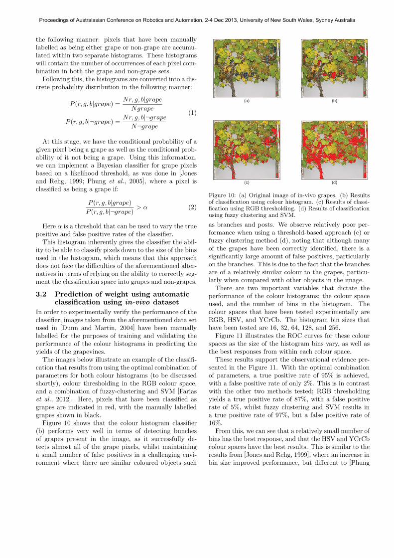
The images below illustrate an example of the classifi-cation that results from using the optimal combination ofparameters for both colour histograms (to be discussedshortly), colour thresholding in the RGB colour space,and a combination of fuzzy-clustering and SVM [Fariaset al., 2012]. Here, pixels that have been classified asgrapes are indicated in red, with the manually labelledgrapes shown in black.

Figure 10 shows that the colour histogram classifier(b) performs very well in terms of detecting bunchesof grapes present in the image, as it successfully de-tects almost all of the grape pixels, whilst maintaininga small number of false positives in a challenging envi-ronment where there are similar coloured objects such

(a) (b)

(c) (d)

Figure 10: (a) Original image of in-vivo grapes. (b) Resultsof classification using colour histogram. (c) Results of classi-fication using RGB thresholding. (d) Results of classificationusing fuzzy clustering and SVM.

as branches and posts. We observe relatively poor per-formance when using a threshold-based approach (c) orfuzzy clustering method (d), noting that although manyof the grapes have been correctly identified, there is asignificantly large amount of false positives, particularlyon the branches. This is due to the fact that the branchesare of a relatively similar colour to the grapes, particu-larly when compared with other objects in the image.

There are two important variables that dictate theperformance of the colour histograms; the colour spaceused, and the number of bins in the histogram. Thecolour spaces that have been tested experimentally areRGB, HSV, and YCrCb. The histogram bin sizes thathave been tested are 16, 32, 64, 128, and 256.

Figure 11 illustrates the ROC curves for these colourspaces as the size of the histogram bins vary, as well asthe best responses from within each colour space.

These results support the observational evidence pre-sented in the Figure 11. With the optimal combinationof parameters, a true positive rate of 95% is achieved,with a false positive rate of only 2%. This is in contrastwith the other two methods tested; RGB thresholdingyields a true positive rate of 87%, with a false positiverate of 5%, whilst fuzzy clustering and SVM results ina true positive rate of 97%, but a false positive rate of16%.

From this, we can see that a relatively small number ofbins has the best response, and that the HSV and YCrCbcolour spaces have the best results. This is similar to theresults from [Jones and Rehg, 1999], where an increase inbin size improved performance, but different to [Phung


0 0.1 0.2 0.3 0.40.75

0.8

0.85

0.9

0.95

1ROC Curves − RGB Colour Space

Tru

e P

ositi

ve R

ate

False Positive Rate

RGB − 16 binsRGB − 32 binsRGB − 64 binsRGB − 128 binsRGB − 256 bins

0 0.1 0.2 0.3 0.40.75

0.8

0.85

0.9

0.95

1ROC Curves − HSV Colour Space

Tru

e P

ositi

ve R

ate

False Positive Rate

HSV − 16 binsHSV − 32 binsHSV − 64 binsHSV − 128 binsHSV − 256 bins

0 0.1 0.2 0.3 0.40.75

0.8

0.85

0.9

0.95

1ROC Curves − YCrCb Colour Space

Tru

e P

ositi

ve R

ate

False Positive Rate

YCrCb − 16 binsYCrCb − 32 binsYCrCb − 64 binsYCrCb − 128 binsYCrCb − 256 bins

0 0.1 0.2 0.3 0.40.85

0.9

0.95

1ROC Curves − Best Responses

Tru

e P

ositi

ve R

ate

False Positive Rate

RGB − 32 binsHSV − 16 binsYCrCb − 16 binsYCrCb − 32 bins

Figure 11: Effect of colour space and bin size on pixel classi-fication accuracy

0 2 4 6 8 10 12 14 16x 10

4

−0.5

0

0.5

1

1.5

2

2.5

3

3.5

4

Automatically Classified Pixel Counts

Bun

ch W

eigh

ts (

kg/m

)

Correlation between Pixel Counts and Bunch Weights

Figure 12: Correlation between pixel counts and bunchweights

et al., 2005], where optimal performance was achievedwith the smallest bin size. [Phung et al., 2005] suggeststhat this is possibly due to the fact that the trainingsets used in this work and in [Jones and Rehg, 1999] arecomparatively small, resulting in poor results for a largenumber of bins due to the fact that much of the colourspace has not been well represented.

Note that another advantage of using a smaller num-ber of bins is the reduction in memory requirements dueto not having to store the larger histograms.

As discussed above, we are most interested in the cor-relation between the number of grape pixels detectedin an image and the weights of the bunches of grapespresent in that image. In this regard, the results of ourpreliminary analysis are very promising. When usingthe classifier discussed above, we obtained the resultsshown in Figure 12 for the correlation between the num-ber of automatically classified pixels and the weights ofthe grape bunches.

Here we have demonstrated that the number of de-

tected pixels using the proposed method of pixel clas-sification is able to account for more than 93% of thevariation in the weights of the grape bunches. This is upfrom 85% that was achieved in [Dunn and Martin, 2004]

using the same data set. This improvement is due to thefact that the method used in [Dunn and Martin, 2004]

is based on applying thresholds across the RGB colourspace. It is interesting to note that the performance ofthe automatic classification is very slightly better thanthat of the manual classification, which is most likelydue to the fact that the automatic classification has beenconducted on a limited data set.

In order to further quantify the predictive power ofthe proposed approach, the average error between thepredicted and actual weights has been calculated usingleave-one-out cross-validation (ignoring images wherethere are only very small amounts of grapes due to ex-cessive relative errors) to be 4.46%. This relates well tothe winemakers target of 5% error and shows that thereis indeed great potential for automatic grape classifica-tion that is capable of accurately predicting the yields ofgrapevines.

4 Conclusion

This preliminary analysis suggests that there is greatpotential for automatic image processing to be used toimprove the accuracy of grape vine yield estimates overexisting manual methods of forecasting, with consequenteconomic benefits.

The results showed that a linear regression approachto bunch weight estimation using berry number, bunchperimeter, bunch area and estimated bunch volume wasaccurate to within 5.3% in ideal conditions whereas byonly using berry number the accuracy decreased to 7.1%.Results from in vivo colour classification showed a weightprediction accuracy of 4.5%, however this made use of avery limited dataset and further field tests are plannedfor the current growing season.

Robust pixel-classification methods have also beendemonstrated to be more accurate than colour thresh-olding, as well as increasing the ability to estimate theweights of grape bunches. Currently only a limited num-ber of image processing and pixel classification method-ologies have been surveyed and this will be expanded infuture work. The sensitivity of classification to variationin the colour space and bin size in different environmen-tal conditions will also be investigated.

One of the critical factors that will dictate the long-term success of this research will be the ability of themethods proposed and tested to be implemented in areal-world system. All bunches analysed in this pa-per have been post-veraison and close to harvest whenmanual sampling is currently used for yield estimation.Going forward, it is planned that entire vineyards will


be surveyed and images collected for use in the grapeclassification. Currently, only a very small percentage(<0.2%) of vines area very small percentage (<0.2%)of vines is sampled using manual methods. By using amuch larger sample size, it is anticipated that much moreaccurate yield estimates will be possible.

Acknowledgments

The authors would like to thank Angus Davidson, PaulPetrie and Gregory Dunn for providing raw image dataand insight into the yield estimation process.

References[Cristofolini and Gottardini, 2000] F. Cristofolini and

E. Gottardini. Concentration of airborne pollen ofVitisvinifera L. and yield forecast: a case studyat S.Michele all’Adige, Trento, Italy. Aerobiologia,16:171–216, 2000.

[Wulfsohn et al., 2012] D. Wulfsohn, F. AravenaZamora, C. Potin Tellez, I. Zamora Lagos, and M.Garcıa-Finana. Multilevel systematic sampling to es-timate total fruit number for yield forecasts. PrecisionAgriculture, 13:256–257, 2012.

[Baldwin, 1964] J. Baldwin. The relation betweenweather and fruitfulness of the sultana vine. Aus-tralian Journal of Agricultural Research, 15:920–928,1964.

[Kastens et al., 2005] J. H. Kastens, T. L. Kastens, D.L. A. Kastens, K. P. Price, E. A. Martinko, and R.-Y.Lee. Image masking for crop yield forecasting usingAVHRR NDVI time series imagery. Remote Sensingof Environment, 99:341–356, 2005.

[Bastiaanssen and Ali, 2003] W. G. M. Bastiaanssenand S. Ali. A new crop yield forecasting model basedon satellite measurements applied across the IndusBasin, Pakistan. Agriculture, Ecosystems & Environ-ment, 94:321–340, 2003.

[Doraiswamy et al., 2005] P. C. Doraiswamy, T. R. Sin-clair, S. Hollinger, B. Akhmedov, A. Stern, and J.Prueger. Application of MODIS derived parametersfor regional crop yield assessment. Remote Sensing ofEnvironment , 97:192–202, 2005.

[Begue et al., 2010] A. Begue, V. Lebourgeois, E. Bap-pel, P. Todoroff, A. Pellegrino, F. Baillarin, et al..Spatio-temporal variability of sugarcane fields and rec-ommendations for yield forecast using NDVI. Interna-tional Journal of Remote Sensing, 31:5391–5407, 2010.

[Weissteiner and Kuhbauch, 2005] C. J. Weissteiner andW. Kuhbauch. Regional Yield Forecasts of MaltingBarley (Hordeum vulgare L.) by NOAA-AVHRR Re-mote Sensing Data and Ancillary Data. Journal ofAgronomy and Crop Science, 191:308–320, 2005.

[Cunha et al., 2010] M. Cunha, A. R. S. Maral, and L.Silva. Very early prediction of wine yield based onsatellite data from Vegetation. International Journalof Remote Sensing, 31:3125–3142, 2010.

[Dunn and Martin, 2004] G. M. Dunn and S. R. Martin.Yield prediction from digital image analysis: A tech-nique with potential for vineyard assessments prior toharvest. Australian Journal of Grape and Wine Re-search, 10:196–198.

[Bjurstrom and Svensson, 2002] H. Bjurstrom and J.Svensson. Assessment of Grapevine Vigour Using Im-age Processing. Masters Thesis, Department of Elec-trical Engineering, Linkoping University, 2002.

[Reis et al., 2012] M. J. C. S. Reis, R. Morais, E. Peres,C. Pereira, O. Contente, S. Soares, et al.. Automaticdetection of bunches of grapes in natural environmentfrom color images. Journal of Applied Logic, 10:285–290, 2012.

[Chamelat et al., 2006] R. Chamelat, E. Rosso, A.Choksuriwong, C. Rosenberger, H. Laurent, andP. Bro. Grape Detection By Image Processing.IECON 2006–32nd Annual Conference, pages 3697–3702, 2006. IEEE Industrial Electronics.

[Diago et al., 2012] M. P. Diago, C. Correa, B. Millan,P. Barreiro, C. Valero, and J. Tardaguila GrapevineYield and Leaf Area Estimation Using SupervisedClassification Methodology on RGB Images Taken un-der Field Conditions. Sensors, 12:16988–17006, 2012.

[Farias et al., 2012] C. Correa Farias, C. Valero Ubierna,and P. Barreiro Elorza. Characterization of vineyard’scanopy through fuzzy clustering and svm over colorimages. 2012.

[Rabatel and Guizard, 2007] G. Rabatel and C.Guizard. Grape berry calibration by computer visionusing elliptical model fitting. Presented at the 6th Eu-ropean Conference on Precision Agriculture, Skiathos,Greece, 2007.

[Nuske et al., 2011] S. Nuske, S. Achar, T. Bates, S.Narasimhan, and S. Singh. Yield estimation in vine-yards by visual grape detection. IEEE/RSJ In-ternational Conference, pages 2352–2358. IntelligentRobots and Systems (IROS).

[Loy and Zelinsky, 2003] G. Loy and A. Zelinsky. Fastradial symmetry for detecting points of interest. IEEETransactions, 25:959-973, 2003. Pattern Analysis andMachine Intelligence.

[Nuske et al., 2012] S. Nuske, K. Gupta, S. Narasimhan,and S. Singh. Modeling and Calibrating Visual YieldEstimates in Vineyards. Proceedings of InternationalConference on Field and Service Robotics, 2012.


[Martin and Dunn, 2001] S. Martin and G. Dunn. CropDevelopment, Crop Estimation and Crop Control toSecure Quality and Production of Major Wine GrapeVarieties: A National Approach. 2001.

[Jones and Rehg, 1999] M. J. Jones and J. H. Rehg. Sta-tistical Color Models with Application to Skin Detec-tion. IEEE Computer Society Conference on Com-puter Vision and Pattern Recognition, 1999.

[Phung et al., 2005] S. L. Phung, A. Bouzerdoum, andD.Chai. Skin Segmentation using Color Pixel Clas-sification: Analysis and Comparison. IEEE Trans-actions, pages 148–154, 2005. Pattern Analysis andMachine Intelligence.


Documents

Towards Automated Yield Estimation in Viticulture · Towards Automated Yield Estimation in Viticulture Scarlett Liu, ... bers and seasonal predictions which takes sig- ... based on