This article was downloaded by: [University of Connecticut]On: 10 October 2014, At: 06:06Publisher: Taylor & FrancisInforma Ltd Registered in England and Wales Registered Number: 1072954 Registeredoffice: Mortimer House, 37-41 Mortimer Street, London W1T 3JH, UK

International Journal of ComputerMathematicsPublication details, including instructions for authors andsubscription information:http://www.tandfonline.com/loi/gcom20

Torus bifurcations, isolas and chaoticattractors in a simple dengue fevermodel with ADE and temporary crossimmunityMaíra Aguiar a b , Nico Stollenwerk a b & Bob W. Kooi ca Centro de Matemática e Aplicações Fundamentais, Universidadede Lisboa , Avenida Prof. Gama Pinto 2, 1649-003, Lisboa,Portugalb Instituto Gulbenkian de Ciência , Apartado 14, 2781-901, Oeiras,Portugalc Faculty of Earth and Life Sciences, Department of TheoreticalBiology , Vrije Universiteit Amsterdam , De Boelelaan 1087, NL1081 HV, Amsterdam, The NetherlandsPublished online: 18 Nov 2010.

To cite this article: Maíra Aguiar , Nico Stollenwerk & Bob W. Kooi (2009) Torus bifurcations,isolas and chaotic attractors in a simple dengue fever model with ADE and temporary crossimmunity, International Journal of Computer Mathematics, 86:10-11, 1867-1877, DOI:10.1080/00207160902783532

To link to this article: http://dx.doi.org/10.1080/00207160902783532

PLEASE SCROLL DOWN FOR ARTICLE

Taylor & Francis makes every effort to ensure the accuracy of all the information (the“Content”) contained in the publications on our platform. However, Taylor & Francis,our agents, and our licensors make no representations or warranties whatsoever as tothe accuracy, completeness, or suitability for any purpose of the Content. Any opinionsand views expressed in this publication are the opinions and views of the authors,and are not the views of or endorsed by Taylor & Francis. The accuracy of the Contentshould not be relied upon and should be independently verified with primary sourcesof information. Taylor and Francis shall not be liable for any losses, actions, claims,proceedings, demands, costs, expenses, damages, and other liabilities whatsoever orhowsoever caused arising directly or indirectly in connection with, in relation to or arisingout of the use of the Content.

This article may be used for research, teaching, and private study purposes. Anysubstantial or systematic reproduction, redistribution, reselling, loan, sub-licensing,systematic supply, or distribution in any form to anyone is expressly forbidden. Terms &Conditions of access and use can be found at http://www.tandfonline.com/page/terms-and-conditions

Dow

nloa

ded

by [

Uni

vers

ity o

f C

onne

ctic

ut]

at 0

6:06

10

Oct

ober

201

4

International Journal of Computer MathematicsVol. 86, Nos. 10–11, October–November 2009, 1867–1877

Torus bifurcations, isolas and chaotic attractors in a simpledengue fever model with ADE and temporary cross immunity

Maíra Aguiara,b*, Nico Stollenwerka,b and Bob W. Kooic

aCentro de Matemática e Aplicações Fundamentais, Universidade de Lisboa, Avenida Prof. Gama Pinto 2,1649-003 Lisboa, Portugal; bInstituto Gulbenkian de Ciência, Apartado 14, 2781-901 Oeiras, Portugal;cFaculty of Earth and Life Sciences, Department of Theoretical Biology, Vrije Universiteit Amsterdam,

De Boelelaan 1087, NL 1081 HV Amsterdam, The Netherlands

(Received 30 July 2008; final version received 27 January 2009)

We analyse an epidemiological model of competing strains of pathogens and hence differences in transmis-sion for first versus secondary infection due to interaction of the strains with previously aquired immunities,as has been described for dengue fever, is known as antibody dependent enhancement (ADE). These mod-els show a rich variety of dynamics through bifurcations up to deterministic chaos. Including temporarycross-immunity even enlarges the parameter range of such chaotic attractors, and also gives rise to vari-ous coexisting attractors, which are difficult to identify by standard numerical bifurcation programs usingcontinuation methods. A combination of techniques, including classical bifurcation plots and Lyapunovexponent spectra, has to be applied in comparison to get further insight into such dynamical structures. Herewe present for the first time multi-parameter studies in a range of biologically plausible values for dengue.The multi-strain interaction with the immune system is expected to have implications for the epidemiologyof other diseases also.

Keywords: numerical bifurcation analysis; Lyapunov exponents; Z2 symmetry; epidemiology; antibodydependent enhancement (ADE)

2000 AMS Subject Classifications: 34C23; 37G35; 37G40; 37D45; 65P30; 92B05

1. Introduction

Epidemic models are classically phrased in ordinary differential equation (ODE) systems for thehost population divided into classes of susceptible individuals and infected ones (SIS system), orin addition, a class of recovered individuals owing to immunity after an infection to the respectivepathogen (SIR epidemics). The infection term includes a product of two variables, hence a non-linearity which in extended systems can cause complicated dynamics. Although these simpleSIS and SIR models only show equilibria as stationary solutions, they already show non-trivialequilibria arising from bifurcations, and in stochastic versions of the system critical fluctuations atthe critical point. Further refinements of the SIR model in terms of external forcing or distinction ofinfections with different strains of a pathogen, hence classes of (a) individuals infected with one or

*Corresponding author. Email: maira@ptmat.fc.ul.pt

ISSN 0020-7160 print/ISSN 1029-0265 online© 2009 Taylor & FrancisDOI: 10.1080/00207160902783532http://www.informaworld.com

Dow

nloa

ded

by [

Uni

vers

ity o

f C

onne

ctic

ut]

at 0

6:06

10

Oct

ober

201

4

1868 M. Aguiar et al.

another strain, (b) those recovered from the infection by one or another strain, (c) those infectedwith more than one strain, etc. can induce more complicated dynamical attractors, includingequilibria, limit cycles, tori and chaotic attractors.

Classical examples of chaos in epidemiological models are provided by childhood diseaseswith extremely high infection rates, so that a moderate seasonal forcing can generate Feigenbaumsequences of period doubling bifurcations into chaos. Success in analysing childhood diseasesin terms of modelling and data comparison lies in the fact that they are just childhood diseaseswith such high infectivity. Otherwise host populations cannot sustain the respective pathogens.In other infectious diseases much lower forces of infection have to be considered leading tofurther conceptual problems with noise affecting the system more than the deterministic part do.This shows even critical fluctuations with power law behaviour, when considering evolutionaryprocesses of harmless strains of pathogens versus occasional accidents of pathogenic mutants [21].In these circumstances only explicitly stochastic models, of which the classical ODE models aremean field versions, can capture the fluctuations observed in time series data [22].

The situation is again different in multi-strain models, which have attracted attention recently.It has been demonstrated that the interaction of various strains on the infection of the host witheventual cross-immunities or other interactions between host immune system and multiple strainscan generate complicated dynamic attractors. A prime example is dengue fever. A first infectionis often mild or even asymptomatic and leads to life long immunity against this strain. However,a subsequent infection with another strain of the virus often causes clinical complications up tolife threatening conditions and hospitalization, owing to ADE. More on the biology of dengueand its consequences for the detailed epidemiological model structure can be found in Aguiar andStollenwerk [1], including literature on previous modelling attempts. For additional literature ondengue models see also [16]. On the biological evidence for ADE see e.g. [12]. In addition tothe difference in the force of infection between primary and secondary infection, parametrizedby a so-called ADE parameter φ, which has been demonstrated to show chaotic attractors in acertain parameter region, namley only for very high contribution of secondary infected to theforce of infection, another effect, the temporary cross-immunity after a first infection against alldengue virus strains, parametrized by the temporary cross-immunity rate α, shows bifurcationsup to chaotic attractors in a much wider and biologically more realistic parameter region, evenfor lowered contribution of secondary infected to the force of infection. Biologically, secondaryinfected hosts develop severe symptoms much more often than first infected and hence are thenhospitalized, which means they contribute less likely to the force of infection [1].

The model presented in the appendix has been described in detail in [1] and has recentlybeen analysed for a parameter value of α = 2 year−1 corresponding on average to half a yearof biologically plausible temporary cross immunity [2]. At low ADE parameter φ there is astable equilibrium. When increasing φ, this equilibrium bifurcates via a Hopf bifurcation into astable limit cycle and then after further continuation the limit cycle becomes unstable in a torusbifurcation. This torus bifurcation can be located using numerical bifurcation software based oncontinuation methods tracking known equilibria or limit cycles up to bifurcation points [7]. Thecontinuation techniques and the theory behind it are described, e.g. in Kuznetsov [15].

Complementary methods like Lyapunov exponent spectra can also characterize chaotic attractor[18,20], and lead eventually to the detection of coexisting attractors to the main limit cyclesand tori originated from the analytically accessible equilibrium for small φ. Such coexistingstructures are often missed in bifurcation analysis of higher dimensional dynamical systems butare demonstrated to be crucial at times in understanding qualitatively the real world data, asfor example demonstrated previously in a childhood disease study [8]. In such a study first theunderstanding of the deterministic system’s attractor structure is needed, and then eventually theinterplay between attractors mediated by population noise in the stochastic version of the systemgives the full understanding of the data.

Dow

nloa

ded

by [

Uni

vers

ity o

f C

onne

ctic

ut]

at 0

6:06

10

Oct

ober

201

4

International Journal of Computer Mathematics 1869

Here we present for the first time extended results of the bifurcation structure for variousparameter values of the temporary cross immunity α in the region of biological relevance andmulti-parameter bifurcation analysis. In addition to the torus bifurcation route to chaos, this alsoreveals the classical Feigenbaum period doubling sequence and the origin of the so-called isolasolutions.

The different strains of the dengue fever virus are genetically and antigenically very similar, andtherefore cause the confusion in the immune response known as ADE [1]. Hence for the host thedifferent strains look similar, leading to identical parameters in dengue models for the differentstrains, which causes symmetry in the model system. This symmetry of the different strains leads tosymmerty breaking bifurcations of limit cycles, which are rarely described in the epidemiologicalliterature but well known in the biochemical literature, e.g. for coupled identical cells.The interplaybetween different numerical procedures and basic analytic insight in terms of symmetries help tounderstand the attractor structure of multi-strain interactions in the present case of dengue fever,and will contribute to the final understanding of dengue epidemiology including the observedfluctuations in real world data. In the literature the multi-strain interaction leading to deterministicchaos viaADE has been described previously, e.g. [4,10], but neglecting temporary cross immunityand hence getting stuck in rather biologically unrealistic parameter regions, whereas more recentlythe considerations of temporary cross immunity in rather complicated and up to now models, whichare not analysed in great detail but include all kinds of interations, have appeared for the first time[17,24], in this case failing to investigate the possible dynamical structures in more detail.

2. Dynamical system

The multistrain model under investigation can be given as an ODE system

d

dtx = f (x, a) (1)

for the state vector of the epidemiological host classes x := (S, I1, I2, . . . , R)tr and besides otherfixed parameters which are biologically undisputed the parameter vector of varied parametersa = (α, φ)tr , with tr for transpose of a vector or a matrix. For a detailed description of the biologicalcontent of state variables and parameters see [1]. The ODE equations and fixed parameter valuesare given in the appendix. The equilibrium values x∗ are given by the equilibrium conditionf (x∗, a) = 0, respectively, for limit cyclesx∗(t + T ) = x∗(t)with periodT . For chaotic attractorsthe trajectory of the dynamical system reaches in the time limit of infinity the attractor trajectoryx∗(t), equally for tori with irrational winding ratios. In all cases the stability can be analysedconsidering small perturbations �x(t) around the attractor trajectories

d

dt�x = df

dx

∣∣∣∣x∗(t)

· �x. (2)

Here, any attractor is notified by x∗(t), be it an equilibrium, periodic orbit or chaotic attractor. Inthis ODE system the linearized dynamics is given with the Jacobian matrix (df /dx) of the ODEsystem equation (1) evaluated at the trajectory points x∗(t) given in notation of (df /dx)|x∗(t).The Jacobian matrix is analysed for equilibria in terms of eigenvalues to determine stability andthe loss of it at bifurcation points, negative real part indicating stability. For the stability andloss of it for limit cylces Floquet multipliers are more common (essentially the exponentials ofeigenvalues), multipliers inside the unit circle indicating stability, and where they leave eventuallythe unit circle determining the type of limit cycle bifurcations. And for chaotic systems Lyapunov

Dow

nloa

ded

by [

Uni

vers

ity o

f C

onne

ctic

ut]

at 0

6:06

10

Oct

ober

201

4

1870 M. Aguiar et al.

exponents are determined from the Jacobian around the trajectory, positive largest exponentsshowing deterministic chaos, zero largest showing limit cycles including tori, largest smaller zeroindicating fixed points.

2.1 Symmetries

To investigate the bifurcation structure of the system under investigation we first observe thesymmetries due to the multi-strain structure of the model.

These symmetries reflect the similarities of the different strain for the host specific proper-ties modelled here, namely the social contact rate and infectivity and the immune response [1].The observation of symmetries due to the multi-strain structure becomes important for the timebeing for equilibria1 and limit cycles. We introduce the following notation: With a symmetrytransformation matrix S

S :=

⎛⎜⎜⎜⎜⎜⎜⎜⎜⎜⎜⎜⎜⎜⎜⎝

1 0 0 0 0 0 0 0 0 00 0 1 0 0 0 0 0 0 00 1 0 0 0 0 0 0 0 00 0 0 0 1 0 0 0 0 00 0 0 1 0 0 0 0 0 00 0 0 0 0 0 1 0 0 00 0 0 0 0 1 0 0 0 00 0 0 0 0 0 0 0 1 00 0 0 0 0 0 0 1 0 00 0 0 0 0 0 0 0 0 1

⎞⎟⎟⎟⎟⎟⎟⎟⎟⎟⎟⎟⎟⎟⎟⎠

(3)

we have the following symmetry:If

x∗ = (S∗, I ∗

1 , I ∗2 , R∗

1 , R∗2 , S

∗1 , S∗

2 , I ∗12, I

∗21, R

∗)tr(4)

is equilibrium or limit cycle, then also

Sx∗ = (S∗, I ∗

2 , I ∗1 , R∗

2 , R∗1 , S

∗2 , S∗

1 , I ∗21, I

∗12, R

∗)tr(5)

with x∗ equilibrium values or x∗ = x∗(t) limit cycle for all times t ∈ [0, T ]. For the right-handside f of the ODE system equation (1) the kind of symmetry found above is called Z2-symmetrywhen the following equivariance condition holds:

f (Sx, a) = Sf (x, a) (6)

with S a matrix that obeys S �= I and S2 = I, where I is the unit matrix. Observe that besidesS I also satisfies Equation (6). The symmetry transformation matrix S in Equation (3) fulfillsthese requirements. It is easy to verify that the Z2-equivariance conditions in Equation (6) andthe properties of S are satisfied for our ODE system. In Seydel [23] a simplified version of thefamous Brusselator that shows this type of symmetry is discussed. There, an equilibrium and alsoa limit cycle show a pitchfork bifurcation with symmetry breaking.

An equilibrium x∗ is called fixed when Sx∗ = x∗ (see [15]). Two equilibria x∗, y∗ whereSx∗ �= x∗, are called S-conjugate if their corresponding solutions satisfy y∗ = Sx∗ (and becauseS2 = I also x∗ = Sy∗). For limit cycles a similar terminology is introduced. A periodic solutionis called fixed when Sx∗(t) = x∗(t) and the associated limit cycles are also called fixed [15].

Dow

nloa

ded

by [

Uni

vers

ity o

f C

onne

ctic

ut]

at 0

6:06

10

Oct

ober

201

4

International Journal of Computer Mathematics 1871

There is another type of periodic solution that is not fixed but called symmetric when

Sx∗(t) = x∗(

t + T

2

), (7)

where T is the period. Again the associated limit cycles are also called symmetric. Both typesof limit cycles L are S-invariant as curves: SL = L. That is, in the phase-plane where timeparameterizes the orbit, the cycle and the transformed cycle are equal. A S-invariant cycle iseither fixed or symmetric. Two noninvariant limit cycles (SL �= L) are called S-conjugate if theircorresponding periodic solutions satisfy y∗(t) = Sx∗(t), ∀t ∈ R. The properties of the symmetricsystems and the introduced terminology are used below with the interpretation of the numericalbifurcation analysis results. We refer to [15] for an overview of the possible bifurcations ofequilibria and limit cycles of Z2-equivariant systems.

3. Bifurcation diagrams for various α values

We show the results of the bifurcation analysis in bifurcation diagrams for several α values,varying φ continuously. In addition to the previously investigated case of α = 2 year−1, we showalso a case of smaller and a case of larger α value, obtaining more information on the bifurcationspossible in the model as a whole. The above-mentioned symmetries help in understanding thepresent bifurcation structure.

3.1 Bifurcation diagram for α = 3

For α = 3 the one-parameter bifurcation diagram is shown in Figure 1(a). Starting with φ = 0there is a stable fixed equilibrium, fixed in the above-mentioned notion for symmetric systems. Thisequilibrium becomes unstable at a Hopf bifurcation H at φ = 0.16445. A stable fixed limit cycleoriginates at this Hopf bifurcation. This limit cycle shows a supercritical pitch-fork bifurcationP −, i.e. a bifurcation of a limit cycle with Floquet multiplier 1, splitting the original limit cycle intotwo new ones. In addition to the now unstable branch two new branches originate for the pair ofconjugated limit cycles. The branches merge again at another supercritical pitch-fork bifurcation

Figure 1. (a) α = 3. Equilibria or extremum values for limit cycles for logarithm of total infected I1 + I2 + I12 + I21.Solid lines denote stable equilibria or limit cycles, dashed lines unstable equilibria or periodic-one limit cycles. Hopfbifurcation H around φ = 0.16 two pitchfork bifurcations P − and a torus bifurcation TR. In addition to this mainbifurcation structure we found coexisting tangent bifurcations T between which some of the isolas live, see especiallythe one between φ = 0.71 and 0.79. Additionally found flip bifurcations are not marked here, see text. (b) α = 2. Inthis case we have a Hopf bifurcation H at φ = 0.11, and besides the similar structure found in (a) also more separatedtangent bifurcations T exist at φ = 0.494, 0.539, 0.931, 0.978 and 1.052, (c) α = 1. Here we have the Hopf bifurcationat φ = 0.0598 and thereafter many tangent bifurcations T , again with coexisting limit cylces.

Dow

nloa

ded

by [

Uni

vers

ity o

f C

onne

ctic

ut]

at 0

6:06

10

Oct

ober

201

4

1872 M. Aguiar et al.

P −, after which the limit cycle is stable again for higher φ-values. The pair of S-conjugate limitcycles become unstable at a torus bifurcation TR at φ = 0.89539.

In addition to this main bifurcation pattern we found two isolas, that is an isolated solutionbranch of limit cycles [11]. These isola cycles L are not S-invariant, that is SL �= L. Isolasconsisting of isolated limit cycles exist between two tangent bifurcations. One isola consists of astable and an unstable branch. The other one shows more complex bifurcation patterns. There isno fully stable branch. For φ = 0.60809 at the tangent bifurcation T , a stable and an unstable limitcycle collide. The stable branch becomes unstable via a flip bifurcation or a periodic doublingbifurcation F , with Floquet multiplier (−1), at φ = 0.61918, which is also a pitchfork bifurcationfor the period-two limit cycles. At the other end of that branch at the tangent bifurcation T atφ = 0.89768 both colliding limit cycles are unstable. Close to this point at one branch thereis a torus bifurcation TR, also called Neimark–Sacker bifurcation, at φ = 0.89539 and a flipbifurcation F at φ = 0.87897, which is again a pitchfork bifurcation P for the period-two limitcycles. Continuation of the stable branch originating for the flip bifurcation F at φ = 0.61918gives another flip bifurcation F at φ = 0.62070 and one close to the other end at φ = 0.87897,namely at φ = 0.87734. These results suggest that for this isola two classical routes to chaos canexist, namely via the torus or Neimark–Sacker bifurcation, where the dynamics on the originatingtorus is chaotic, and the cascade of period doubling route to chaos.

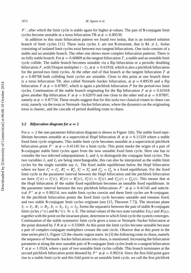
3.2 Bifurcation diagram for α = 2

For α = 2 the one-parameter bifurcation diagram is shown in Figure 1(b). The stable fixed equi-librium becomes unstable at a supercritical Hopf bifurcation H at φ = 0.11329 where a stablefixed limit cycle originates. This stable limit cycle becomes unstable at a superciritcal pitchforkbifurcation point P − at φ = 0.41145 for a limit cycle. This point marks the origin of a pair ofS-conjugate stable limit cycles apart from the now unstable fixed limit cycle. Here one has toconsider the two infected subpopulations I1 and I2 to distinguish the conjugate limit cycles. Thetwo variables I1 and I2 are being interchangeable, this can also be interpreted as the stable limitcycles for the single variable say I1. The fixed stable equilibrium below the Hopf bifurcationwhere we have I ∗

1 = I ∗2 , R∗

1 = R∗2 , S∗

1 = S∗2 and I ∗

12 = I ∗21 is a fixed equilibrium. For the fixed

limit cycle in the parameter interval between the Hopf bifurcation and the pitchfork bifurcationwe have I ∗

1 (t) = I ∗2 (t), R∗

1(t) = R∗2(t), S∗

1 (t) = S∗2 (t) and I ∗

12(t) = I ∗21(t). This means that at

the Hopf bifurcation H the stable fixed equilibrium becomes an unstable fixed equilibrium. Inthe parameter interval between the two pitchfork bifurcations P − at φ = 0.41145 and subcrit-ical P + at φ = 0.99214, two stable limit cycles coexist and these limit cycles are S-conjugate.At the pitchfork bifurcation points the fixed limit cycle becomes unstable and remains fixed,and two stable S-conjugate limit cycles originate (see [15, Theorem 7.7]). The invariant planeI1 = I2, R1 = R2, S1 = S2, I12 = I21 forms the separatrix between the pair of stable S-conjugatelimit cycles x∗(t) and Sx∗(t), ∀t ∈ R. The initial values of the two state variables S(t0) and R(t0),together with the point on the invariant plane, determine to which limit cycle the system converges.Continuation of the stable symmetric limit cycle gives a torus or Neimark–Sacker bifurcation atthe point denoted by T R at φ = 0.55069. At this point the limit cycles become unstable becausea pair of complex-conjugate multipliers crosses the unit circle. Observe that at this point in thetime series plot [1, Figure 12] the chaotic region starts. In [3] the following route to chaos, namelythe sequence of Neimark–Sacker bifurcations into chaos, is mentioned. Increasing the bifurcationparameter φ along the now unstable pair of S-conjugate limit cycles leads to a tangent bifurcationT at φ = 1.0524, where a pair of two unstable limit cycles collide. This branch terminates at thesecond pitchfork bifurcation point denoted by P + at φ = 0.99214. Since the first fold point gaverise to a stable limit cycle and this fold point to an unstable limit cycle, we call the first pitchfork

Dow

nloa

ded

by [

Uni

vers

ity o

f C

onne

ctic

ut]

at 0

6:06

10

Oct

ober

201

4

International Journal of Computer Mathematics 1873

bifurcation supercritical and the latter pitchfork bifurcation subcritical. These results agree verywell with the simulation results shown in the bifurcation diagram for the maxima and minimaof the overall infected (see Figure 15 in [1]). Notice that AUTO [7] calculates only the globalextrema during a cycle, not the local extrema. Figure 1(b) shows also two isolas similar to thosefor α = 3 in Figure 1(a).

3.3 Bifurcation diagram for α = 1

For α = 1 the bifurcation diagram is shown in Fig. 1(c). In the lower φ parameter range there isbistability of two limit cycles in an interval bounded by two tangent bifurcations T . The stablemanifold of the intermediate saddle limit cycle acts as a separatrix. Inceasing φ the stable limitcycles become unstable at the pitchfork bifurcation P at φ = 0.23907. Following the unstable pri-mary branch, for larger values of φ we observe an open loop bounded by two tangent bifurcationsT . The extreme value for φ is at φ = 0.62790. Then lowering φ there is a pitchfork bifurcationP at φ = 0.50161. Later we will return to the description of this point. While lowering φ furtherthe limit cycle becomes stable again at the tangent bifurcations T at φ = 0.30863. On increasingφ this limit cycle becomes unstable again at the pitchfork bifurcation P at φ = 0.32532.

Continuation of the secondary branch of the two S-conjugated limit cycles from this pointreveals that the stable limit cycle becomes unstable at a torus bifurcation TR at φ = 0.42573.The simulation results depicted in [1, Figure 13] show that there is chaos beyond this point.The secondary pair of S-conjugate limit cycles that originate from pitchfork bifurcation P atφ = 0.23907 becomes unstable at a flip bifurcation F . Increasing φ further it becomes stableagain at a flip bifurcation F . Below we return to the interval between these two flip bifurcations.The stable part becomes unstable at a tangent bifurcation T , then continuing, after a tangentbifurcation T and a Neimark–Sacker bifurcation TR. This bifurcation can lead to a sequenceof Neimark–Sacker bifurcations into chaos. The unstable limit cycles terminates via a tangentbifurcation F where the primary limit cycle possesses a pitchfork bifurcation P at φ = 0.50161.At the flip bifurcation F the cycle becomes unstable and a new stable limit cycle with doubleperiod emanates. The stable branch becomes unstable at a flip bifurcation again. We concludethat there is a cascade of period doubling route to chaos. Similarly this happens in reversed orderending at the flip bifurcation where the secondary branch becomes stable again.

Figure 2(a) gives the results for the interval 0.28 ≤ φ ≤ 0.44, where only the minima areshown. In this plot also a ‘period three’ limit cycle is shown. In a small region it is stable andcoexists together with the ‘period one’ limit cycle. The cycles are shown in Figure 2(b) and (c)for φ = 0.294. The one in Figure 2(c) looks like a period-3 limit cycle. In Figure 2 continuation

Figure 2. (a) α = 1. Detail of Figure 1(c). We find pitchfork bifurcations P at φ = 0.239 and 0.325, flip bifurcations F

at φ = 0.298, 0.328,0.344,0.346, 0.406, 0.407, 0.411 and 0.422, further tangent bifurcations T at φ = 0.292, 0.346 and0.422. Four almost coexisting bifurcations, namely F ’s at φ = 0.4112590. (b) and (c) state space-plots of susceptiblesand logarithm of infected for α = 1 and φ = 0.294 for two coexisting stable limit cycles.

Dow

nloa

ded

by [

Uni

vers

ity o

f C

onne

ctic

ut]

at 0

6:06

10

Oct

ober

201

4

1874 M. Aguiar et al.

of the limit cycle gives a closed graph bounded at the two ends by tangent bifurcations T , wherea stable and an unstable limit cycles collide. The intervals where the limit cycle is stable, areon the other end bounded by flip bifurcations F . One unstable part intersects the higher periodcycles that originate via the cascade of period doubling between the period-1 limit cycle flipbifurcations F at φ = 0.32816 and 0.41126. This suggest that the period-3 limit cycle is associatedwith a ‘period-3 window’ of the chaotic attractor. We conjecture that this interval is boundedby two homoclinic bifurcations for a period-3 limit cycle [5,6,13,14]. The bifurcation diagramshown in [1, Figure 13] shows the point where the chaotic attractor disappears abruptly, possibleat one of the two homoclinic bifurcations. In that region the two conjugated limit cycles thatoriginate at the pitchfork bifurcation P at φ = 0.32532 are the attractors. These results suggestthat there are chaotic attractors associated with the period-1 limit cycle, one occurs via a cascadeof flip bifurcations originating from the two ends at φ = 0.32816 and φ = 0.41126 and one viaa Neimark–Sacker bifurcation T R at φ = 0.42573.

4. Two-parameter diagram

We will now link the three studies of the different α values by investigating a two-parameterdiagram for φ and α, concentrating especially on the creation of isolated limit cycles, whichsometimes lead to further bifurcations inside the isola region. Figure 3 gives a two-parameterbifurcation diagram where φ and α are the free parameters. For low φ-values there is the Hopfbifurcation H and all other curves are tangent bifurcation curves.

Isolas appear or disappear upon crossing an isola variety. At an elliptic isola point an isolatedsolution branch is born, while at a hyperbolic isola point an isolated solution branch vanishes bycoalescence with another branch [11]. From Figure 3 we see that at two values of α > 3 isolasare born. Furthermore, period doubling bifurcations appear for lower α values, indicating the

Figure 3. Two-dimensional parameter bifurcation diagram with φ and α as parameters. Only one Hopf bifurcation(dotted line) and many tangent bifurcation curves for limit cycles (dashed lines) are shown in the range α ∈ [1, 3.8]. Theisolated limit cycles originate above α = 3. For lower values of α periodic doubling routes to chaos originate.

Dow

nloa

ded

by [

Uni

vers

ity o

f C

onne

ctic

ut]

at 0

6:06

10

Oct

ober

201

4

International Journal of Computer Mathematics 1875

Figure 4. Spectrum of the four largest Lyapunov exponents with changing parameter φ and α fixed to the followingvalues: (a) α = 4, (b) α = 2 and (c) α = 1.

Feigenbaum route to chaos. However, only the calculation of Lyapunov exponents, which arediscussed in the next section, can clearly indicate chaos.

5. Lyapunov spectra for various α values

The Lyapunov exponents are the logarithms of the eigenvalues of the Jacobian matrix along theintegrated trajectories, Equation (2), in the limit of large integration times. With the exception ofvery simple iterated maps no analytic expressions for chaotic systems exists for the Lyapunovexponents. For the calculation of the iterated Jacobian matrix and its eigenvalues, we use the QRdecomposition algorithm [9,19].

In Figure 4 we show the four largest Lyapunov exponents in the φ range between zero andone for various α values. For α = 4 in Figure 4(a) we see for small φ values a fixed pointbehaviour indicated by a negative largest Lyapunov exponent up to around φ = 0.2. There, atthe Hopf bifurcation point, the largest Lyapunov exponent becomes zero, indicating limit cyclebehaviour for the whole range of φ, apart from the final bit before φ = 1, where a small spikewith positive Lyapunov exponent might be present, but difficult to distinguish from the noisynumerical background.

For α = 2 in Figure 4(b) however, we see a large window with positive largest Lyapunov expo-nent, well separated from the second largest one being zero. This is a clear sign of deterministicallychaotic attractors being present for this φ range. Just a few windows with periodic attractors, indi-cated by the zero, largest Lyapunov exponents are visible in the region of 0.5 < φ < 1. For smallerφ values we observe qualitatively the same behaviour as already seen for α = 4. For the smallervalue of α = 1 in Figure 4(c) the chaotic window is even larger than for α = 2. Hence determin-istic chaos is present for temporary cross immunity in the range around α = 2 year−1 and for φ

between zero and one.

6. Conclusions

We have presented a detailed bifurcation analysis for a multi-strain dengue fever model in terms ofthe ADE parameter φ, in the previously not very well-investigated region between zero and one,and a parameter for the temporary cross immunity α. The symmetries implied by the strain struc-ture are taken into account in the analysis. Many of the possible bifurcations of equilibria and limitcycles of Z2-equivariant systems can be distinguished. Using AUTO [7] the different dynamicalstructures were calculated and coexisting attractors detected. In stochastic versions of the present

Dow

nloa

ded

by [

Uni

vers

ity o

f C

onne

ctic

ut]

at 0

6:06

10

Oct

ober

201

4

1876 M. Aguiar et al.

model [1] such coexisting attractors and eventually even transient chaos can be visited by thesame system, leading to rather a more complicated dynamical behaviour than simpler one [8].

Future time series analysis of epidemiological data has good chances to give insight into therelevant parameter values purely on topological information of the dynamics, rather than by usingthe classical parameter estimation of which application is in general restricted to fairly simpledynamical scenarios.

Acknowledgements

This work has been supported by the European Union under the Marie Curie grant MEXT-CT-2004-14338. We thankGabriela Gomes and Luis Sanchez, Lisbon, for scientific support.

Note

1. Equilibria are often called fixed points in dynamical systems theory; here we try to avoid this term, since in symmetrythe term fixed is used in a more specific way.

References

[1] M. Aguiar and N. Stollenwerk, A new chaotic attractor in a basic multi-strain epidemiological model with temporarycross-immunity arXiv:0704.3174v1 [nlin.CD] (2007). Available at http://arxive.org.

[2] M. Aguiar, B.W. Kooi, and N. Stollenwerk, Epidemiology of dengue fever: A model with temporary cross-immunityand possible secondary infection shows bifurcations and chaotic behaviour in wide parameter regions, Math. Model.Nat. Phenom. 3 (2008), pp. 48–70.

[3] D. Albers and J. Sprott, Routes to chaos in high-dimensional dynamical systems: a qualitative numerical study,Physica D 223 (2006), pp. 194–207.

[4] L. Billings, B.I. Schwartz, B.L. Shaw, M. McCrary, D.S. Burke, and T.A.D. Cummings, Instabilities in multiserotypedisease models with antibody-dependent enhancement, J. Theoret. Biol. 246 (2007), pp. 18–27.

[5] M.P. Boer, B.W. Kooi, and S.A.L.M. Kooijman, Homoclinic and heteroclinic orbits in a tri-trophic food chain,J. Math. Biol. 39 (1999), pp. 19–38.

[6] M.P. Boer, B.W. Kooi, and S.A.L.M. Kooijman, Multiple attractors and boundary crises in a tri-trophic food chain,Math. Biosci. 169 (2001), pp. 109–128.

[7] E.J. Doedel, R.C. Paffenroth, A.R. Champneys, T.F. Fairgrieve, Y.A. Kusnetsov, B. Sandstede, B. Oldeman, X.J.Wang, and C. Zhang, AUTO 07P – Continuation and bifurcation software for ordinary differential equations, Tech.Rep.: Concordia University, Montreal, Canada (2007). Available at http://indy.cs.concordia.ca/auto/

[8] F.R. Drepper, R. Engbert, and N. Stollenwerk, Nonlinear time series analysis of empirical population dynamics,Ecol. Modelling 75/76 (1994), pp. 171–181.

[9] J.P. Eckmann, S. Oliffson-Kamphorst, D. Ruelle, and S. Ciliberto, Liapunov exponents from time series, Phys. Rev.A 34 (1986), pp. 4971–4979.

[10] N. Ferguson, R.Anderson, and S. Gupta, The effect of antibody-dependent enhancement on the transmission dynamicsand persistence of multiple-strain pathogens, Proc. Natl. Acad. Sci. USA 96 (1999), pp. 790–794.

[11] M. Golubitsky and D.G. Schaeffer, Singularities and Groups in Bifurcation Theory, Springer, New York, 1985.[12] S.B. Halstead, Neutralization and antibody-dependent enhancement of dengue viruses, Adv. Virus Res. 60 (2003),

pp. 421–467.[13] B.W. Kooi and M.P. Boer, Chaotic behaviour of a predator-prey system, Dyn. Contin. Discrete Impuls. Syst., Ser.

B: Appl. Algorithms 10 (2003), pp. 259–272.[14] B.W. Kooi, L.D.J. Kuijper, and S.A.L.M. Kooijman, Consequence of symbiosis for food web dynamics, J. Math.

Biol. 49 (2004), pp. 227–271.[15] Y.A. Kuznetsov, Elements of Applied Bifurcation Theory,Applied Mathematical Sciences, vol. 112, 3rd ed., Springer-

Verlag, New York, 2004.[16] E. Massad, M. Chen, S. Ma, C.J. Struchiner, N. Stollenwerk, and M. Aguiar, Scale-free network for a dengue

epidemic, Appl. Math. Comput. 159 (2008), pp. 376–381.[17] Y. Nagao and K. Koelle, Decreases in dengue transmission may act to increase the incidence of dengue hemorrhagic

fever, Proc. Natl. Acad. Sci. USA 105 (2008), pp. 2238–2243.[18] E. Ott, Chaos in Dynamical Systems, Cambridge University Press, Cambridge, 2002.[19] U. Parlitz, Identification of true and spurious Lyapunov exponents from time series, Int. J. Bifur. Chaos 2 (1992),

pp. 155–165.[20] D. Ruelle, Chaotic Evolution and Strange Attractors, Cambridge University Press, Cambridge, 1989.

Dow

nloa

ded

by [

Uni

vers

ity o

f C

onne

ctic

ut]

at 0

6:06

10

Oct

ober

201

4

International Journal of Computer Mathematics 1877

[21] N. Stollenwerk and V.A.A. Jansen, Evolution towards criticality in an epidemiological model for meningococcaldisease, Phys. Lett. A 317 (2003), pp. 87–96.

[22] N. Stollenwerk, M.C.J. Maiden, and V.A.A. Jansen, Diversity in pathogenicity can cause outbreaks of menigococcaldisease, Proc. Natl. Acad. Sci. USA 101 (2004), pp. 10229–10234.

[23] R. Seydel, Practical Bifurcation and Stability Analysis-from Equilibrium to Chaos, Springer-Verlag, New York,1994.

[24] H.J. Wearing and P. Rohani, Ecological and immunological determinants of dengue epidemics, Proc. Natl. Acad.Sci. USA 103 (2006), pp. 11802–11807.

Appendix A. Epidemic model equations

The complete system of ODEs for a two strain epidemiological system allowing for differences in primary versus secondaryinfection and temporary cross immunity is given by

d

dtS = − β

NS(I1 + φI21) − β

NS(I2 + φI12) + μ(N − S),

d

dtI1 = β

NS(I1 + φI21) − (γ + μ)I1,

d

dtI2 = β

NS(I2 + φI12) − (γ + μ)I2,

d

dtR1 = γ I1 − (α + μ)R1,

d

dtR2 = γ I2 − (α + μ)R2,

d

dtS1 = − β

NS1(I2 + φI12) + αR1 − μS1,

d

dtS2 = − β

NS2(I1 + φI21) + αR2 − μS2,

d

dtI12 = β

NS1(I2 + φI12) − (γ + μ)I12,

d

dtI21 = β

NS2(I1 + φI21) − (γ + μ)I21,

d

dtR = γ (I12 + I21) − μR.

(A.1)

For two different strains, 1 and 2, we label the SIR classes for the hosts that have seen the individual strains. Susceptibles toboth strains (S) get infected with strain 1 (I1) or strain 2 (I2), with infection rate β. They recover from infection with strain1 (becoming temporary cross-immune R1) or from strain 2 (becoming R2), with recovery rate γ , and so on. With rate α,the R1 and R2 enter again in the susceptible classes (S1 being immune against strain 1 but susceptible to 2, respectively,S2), where the index represents the first infection strain. Now, S1 can be reinfected with strain 2 (becoming I12), meetingI2 with infection rate β or meeting I12 with infection rate φβ, secondary infected contributing differently to the force ofinfection than primary infected, and so on.

We include demography of the host population denoting the birth and death rate by μ. For constant population size N

we have for the immune to all strains R = N − (S + I1 + I2 + R1 + R2 + S1 + S2 + I12 + I21) and therefore we onlyneed to consider the first nine equations of Equation (A.1), giving nine Lyapunov exponents. In our numerical studies wetake the population size N = 100 so that mean proportions of susceptibles, infected, etc. are given in percentage. As fixedparameter values we take μ = ( 1

65 ) year−1, γ = 52 year−1, β = 2 · γ . The parameters φ and α are varied.

Dow

nloa

ded

by [

Uni

vers

ity o

f C

onne

ctic

ut]

at 0

6:06

10

Oct

ober

201

4