Today

Early vision on a single image

Midterm Exam

Starting from 12:00am EST, Tuesday, March 9th in Blackboard

Due: 11:59pm EST, Wednesday, March 10th

A calculator is allowed

Cover everything till the class on Thursday, March 4th

Open book and open notes

Reminder

Homework #2 is due on 11:59pm EST, Thursday, Feb 11th.

Early Vision on One Image

So far, we talked about image formation. Next, we will discuss early vision on one image

• Linear and nonlinear filters

• Linear and nonlinear filters for noise reduction

• Linear filters for differentiation

• Edge detection

• Features

• Edges, lines, curves, corners etc.

Early Vision on One Image

BinaryGray level Color

Binary Image

1 1 1

0: Black

1: White

p

q

X

Y

0

Row 1

Row q

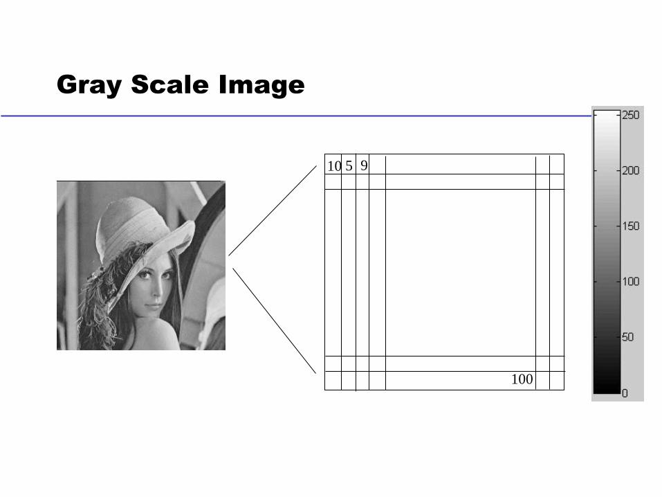
Gray Scale Image

10 5 9

100

Color Image (RGB)B

G

R

Early Vision on One Image: Two Important

Topics

• Image noise: intrinsic property of the sensor (CCD) and independent of scene

• Intensity noise – quantization and sensor

• Positional noise – spatial sampling

Early Vision on One Image: Two Important

Topics

• Features: characterizing the shape/appearance of the objects in the image

• Edges, lines, curves, corners etc.

• Image statistics: mean, variance, histogram etc.

• Complex features

• Widely used in many problems of computer vision including camera calibration, stereo, object detection/tracking/recognition, etc.

Properties of Noise

• Spatial properties

• Spatially periodic noise

• Spatially independent noise

• Frequency properties

• White noise – noise containing all frequencies within a bandwidth

Image Noise

መ𝐼(𝑥, 𝑦) = 𝐼(𝑥, 𝑦) + 𝜂(𝑥, 𝑦)

Image noise

Observed image intensity Ideal image intensity

Some Important Noise Model

𝑝(𝑧) =1

2𝜋𝜎𝑒−(𝑧− lj𝑧)2

2𝜎2

• Due to electronic circuit

• Due to the image sensor

• poor illumination

• high temperature

Most popular noise model

Assumption: the image noise is identically and independently.

Gaussian noise model

Some Important Noise Model

𝑝(𝑧) = ቐ2

𝑏(𝑧 − 𝑎)𝑒−

(𝑧−𝑎)2

𝑏 𝑧 ≥ 𝑎

0 𝑧 < 𝑎𝑝(𝑧) = ൞

𝑎𝑏𝑧𝑏−1

(𝑏 − 1)!𝑒−𝑎𝑧 𝑧 ≥ 0

0 𝑧 < 0

Rayleigh noise

• range imaging

• Background model for Magnetic

Resonance Imaging (MRI) images

Gamma noise

• laser imaging

Figure from “Digital Image Processing”, Gonzalez and Woods

Some Important Noise Model

𝑃(𝑧) =

𝑃𝑎 for 𝑧 = 𝑎𝑃𝑏 for 𝑧 = 𝑏

0 Otherwise

𝑃(𝑧) = ቊ𝑎𝑒−𝑎𝑧 𝑧 ≥ 00 𝑧 < 0 𝑃(𝑧) = ቐ

1

𝑏 − 𝑎𝑎 ≤ 𝑧 ≤ 𝑏

0 𝑜𝑡ℎ𝑒𝑟𝑤𝑖𝑠𝑒

Exponential noise

• laser imaging

Impulse noise

• salt and pepper noise

• A/D converter error

• bit error in transmission

Uniform noise

Figure from “Digital Image Processing”, Gonzalez and Woods

An Example

What is its histogram?

Figure from “Digital Image Processing”, Gonzalez and Woods

An Example (cont.)

Figure from “Digital Image Processing”, Gonzalez and Woods

ExponentialRayleigh GammaGaussian Uniform Salt & Pepper

Another Example

Sigma =1 Sigma =16

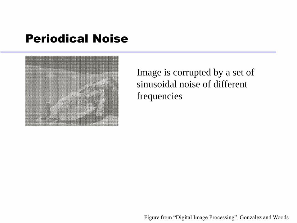
Periodical Noise

Image is corrupted by a set of

sinusoidal noise of different

frequencies

Figure from “Digital Image Processing”, Gonzalez and Woods

Estimation of Noise Parameters

Take a small stripe of the background, do statistics for the mean and variance.

Figure from “Digital Image Processing”, Gonzalez and Woods

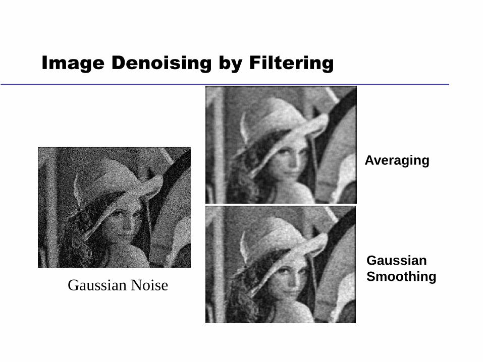
Image Denoising by Filtering

Gaussian Noise

Gaussian

Smoothing

Averaging

Image Filtering

Modifying the pixels in an image based on some function of a local neighborhood of the pixels

10 30 10

20 11 20

11 9 1

p

N(p)

f(p)

𝑓 𝑝

f(p):

• Linear function• Correlation

• Convolution

• Nonlinear function• Order statistic (median)

Linear Filters

General process:

• Form new image whose pixels are a weighted sum of original pixel values, using the same set of weights at each point.

Properties

• Output is a linear function of the input

• Output is a shift-invariant function of the input (i.e. shift the input image two pixels to the left, the output is shifted two pixels to the left)

Example: smoothing by averaging

• form the average of pixels in a neighborhood

Example: smoothing with a Gaussian

• form a weighted average of pixels in a neighborhood

Example: finding an edge

Linear Filtering

The output is the linear combination of the neighborhood pixels

The coefficients of this linear combination combine to form the “filter-kernel”

𝑓 𝑝 =

𝑞𝑖∈𝑁 𝑝

𝑎𝑖𝑞𝑖

1 3 0

2 10 2

4 1 1

Image

1 0 -1

1 0.1 -1

1 0 -1

Kernel

= 5

Filter Output

⊗

Convolution

𝑓 𝑖, 𝑗 = 𝐼 ∗ 𝐻 =

𝑘

𝑙

𝐼 𝑘, 𝑙 𝐻 𝑖 − 𝑘, 𝑗 − 𝑙

𝐼 = Image𝐻 = Kernel

H7 H8 H9

H4 H5 H6

H1 H2 H3

H9 H8 H7

H6 H5 H4

H3 H2 H1

H1 H2 H3

H4 H5 H6

H7 H8 H9

𝐻

𝑋 − 𝑓𝑙𝑖𝑝

𝑌 − 𝑓𝑙𝑖𝑝

I1 I2 I3

I4 I5 I6

I7 I8 I9

⊗

𝐼 ∗ 𝐻 = 𝐼1𝐻9 + 𝐼2𝐻8 + 𝐼3𝐻7

+ 𝐼4𝐻6 + 𝐼5𝐻5 + 𝐼6𝐻4

+ 𝐼7𝐻3 + 𝐼8𝐻2 + 𝐼9𝐻1

𝐼

Linear Filtering

0 0 0

0 1 0

0 0 0

∗=

Linear Filtering

0 0 0

0 0 1

0 0 0

∗=

Linear Filtering (Smoothing)

1 1 1

1 1 1

1 1 1

∗1

9=

Linear Filtering (Blurring)

1 1 1 1 1

1 1 1 1 1

1 1 1 1 1

1 1 1 1 1

1 1 1 1 1

∗1

25=