To the Graduate Council: I am submitting herewith a thesis written by SeongTaek Lee entitled “Design and Analysis of New Concept Interior Permanent Magnet Synchronous Motor by 3D Finite Element Analysis.” I have examined the final electronic copy of this thesis for form and content and recommend that it be accepted in partial fulfillment of the requirements for the degree of Master of Science, with a major in Electrical Engineering. Leon Tolbert Major Professor We have read this thesis and recommend its acceptance: Jack S. Lawler

John Chiasson

Accepted for the Council: Anne Mayhew

Vice Chancellor and Dean of Graduate Studies

(Original signatures are on file with official student records)

Design and Analysis of New Concept Interior Permanent Magnet

Synchronous Motor by 3D Finite Element Analysis

A Thesis

Presented for the

Master of Science

Degree

The University of Tennessee, Knoxville

SeongTaek Lee

August 2005

ii

DEDICATION

This thesis is dedicated to my family; my wife Min-young and daughter Jennifer, and my

mother, who always encouraged me with their love.

iii

ACKNOWLEDGMENTS

I wish to thank all those who helped me in completing my degree. I thank Dr.

Tolbert for his continuous guidance throughout the process of writing my thesis. I thank

all the professors who have contributed to my education at The University of Tennessee.

They have demanded excellence and made me a better engineer. I especially thank Dr.

Lawler and Dr. Chiasson for serving on my committee.

I would also like to thank the National Transportation Research Center at the Oak

Ridge National Laboratory to give me the chance to research there. In particular, I would

like to thank Dr. John Hsu who has supported and encouraged me while I was pursuing

my degree.

iv

ABSTRACT

Throughout the years Hybrid Electric Vehicles (HEV) require an electric motor

which has high power density and wide constant power operating region as well as low

manufacturing cost. For these purposes, a new concept permanent magnet motor is

designed and analyzed with the basic theories about Interior Permanent Magnet

Synchronous Motor (IPMSM).

This new motor has DC excitation coils and flux paths, which can increase the

output torque and be controlled for field weakening operating. The analysis has been

conducted by three-dimensional Finite Element Analysis. The results show the possibility

of the new motor for HEV applications. The new motor has several advantages: low

manufacturing cost, low inertia of the rotor, and the direct controllability of air-gap flux.

v

LIST OF CONTENTS

1. Introduction

1.1. Background ................................................................................................ 1

1.2. Comparison of Electric Motors.................................................................. 3

1.2.1. Induction Motor............................................................................... 3

1.2.2. Permanent Magnet Synchronous Motor.......................................... 4

1.2.3. Switched Reluctance Motor ............................................................ 5

1.3. Research Objective .................................................................................... 6

1.4. Thesis Organization ................................................................................... 8

2. Analysis of Interior Permanent Magnet Synchronous Motor (IPMSM)

2.1. Background ............................................................................................... 9

2.2. Torque Equation from Steady-State Phasor Diagram.............................. 11

2.3. Torque Equation from Magnetic Field Energy ........................................ 17

2.4. Finite Element Analysis – Maxwell 3D .................................................. 21

2.5. Summary .................................................................................................. 25

3. FEA Simulation of the Concept of a New IPMSM

3.1. Introduction ............................................................................................. 26

3.2. Modeling ................................................................................................. 27

3.3. Numerical Analysis.................................................................................. 30

3.4. Simulation Results ................................................................................... 33

vi

4. Design a New Concept Motor

4.1. Design Procedure .................................................................................... 36

4.2. Pre-developed Motor................................................................................ 37

4.2.1. Geometries and materials of pre-developed motor ....................... 37

4.2.2. Simulation results of pre-developed motor .................................. 41

4.3. Embodiment of the Concept ................................................................... 43

4.3.1. Side-poles and side-magnets ........................................................ 43

4.3.2. Excitation flux paths ..................................................................... 49

4.3.3. Excitation coil resistance .............................................................. 49

4.4. Simulation Results of Final Model ......................................................... 53

4.4.1. Air-gap flux .................................................................................. 53

4.4.2. Output torque ................................................................................ 59

4.5. Summary and Discussion......................................................................... 61

5. Conclusions and Future Works

5.1. Conclusions ............................................................................................ 67

5.2. Future Works.......................................................................................... 69

REFERENCES .................................................................................................... 70

APPENDICES

A. Flowchart of Maxwell 3D ......................................................................... 75 B. Park’s transformation and Reference Coordinate systems........................ 76

VITA ............ ....................................................................................................... 78

vii

LIST OF FIGURES

1.1 Required characteristics of traction motor in a vehicle running mode ............. 2

1.2 Speed-Torque curves for variable frequency control of IM.............................. 4

2.1 Various rotor configurations with PM ............................................................ 10

2.2 Phasor diagram for IPMSM ............................................................................ 13

2.3 Torque-angle characteristic of IPMSM........................................................... 16

2.4 A simple rotating machine .............................................................................. 18

2.5 Comparing B-H curve between linear and nonlinear material........................ 24

3.1 Simulation concept model to increase air gap flux ......................................... 27

3.2 FEA simulation result of air-gap flux density of the concept model ............. 28

3.3 Simulation model with side cores and wound coils ........................................ 29

3.4 Simplified model for excited flux path .......................................................... 31

3.5 Simulation results of air-gap flux density for different excitation conditions 34

3.6 B vector on three cut-planes in the simulation model .................................... 35

4.1 A quarter model of pre-developed motor for FEA.......................................... 38

4.2 The location of PMs in the rotor ..................................................................... 39

4.3 B-H curves for non-linear materials................................................................ 40

4.4 Air-gap flux density distribution of pre-developed motor .............................. 41

4.5 Output torque versus current phase angle for pre-developed motor ............... 42

viii

4.6 Configuration of side-poles............................................................................. 44

4.7 Configuration of side-poles and side-magnets ............................................... 45

4.8 Flux density vector distributions around side-pole at centered N-position .... 46

4.9 Magnitude of the flux density on the side-pole and the clamping at centered

N-position....................................................................................................... 47

4.10 Axial flux path of the motor.......................................................................... 48

4.11 Flux density vector distributions on the axial cut plane at N-position.......... 50

4.12 Flux density vector distributions on the axial cut plane at S-position .......... 50

4.13 Simulation results of air-gap flux density for different excitation values..... 54

4.14 Flux density vector distributions at no phase current.................................... 56

4.15 Magnitude of flux density at no phase current.............................................. 56

4.16 Flux density vector distributions at maximum torque position..................... 57

4.17 Magnitude of flux density at maximum torque position .............................. 57

4.18 Overall magnitude of flux density at maximum torque position ................. 58

4.19 Comparison of output torque between pre-developed and final model ........ 59

4.20 Comparison of output torque under various excitation current values ......... 60

4.21 Flux density distributions on the axial cut-plane (Iph,max= 200A, Iexc= 3000At) ....................................................................................................... 63

4.22 Flux density distributions on the axial cut-plane (Iph,max= 200A, Iexc= 0At) ....................................................................................................... 64

4.22 Flux density distributions on the axial cut-plane (Iph,max= 200A, Iexc= -1500At) ....................................................................................................... 65

B.1 A quarter IPMSM model for references of the three-phase ........................... 77

1

CHAPTER 1

Introduction

1.1 Background

Throughout the years hybrid electric vehicles (HEVs) have proved themselves

worthy to replace a conventional vehicle with an internal combustion engine (ICE).

Recently, the commercial HEVs developed by Toyota and Honda have proven about 50%

fuel saving in urban driving in comparison with an equivalent ICE vehicle [1]. This is

great progress, but the fuel saving still cannot compensate for the extra cost of an HEV in

initial purchase and maintenance. Thus, the price and reliability of the traction motor is

one of the most critical issues in developing an HEV system.

Various types of electric motors have been investigated for use in an HEV system

in the fields of output power, maximum speed, efficiency, manufacturing cost, and

durability. Figure 1.1 shows the motor requirements of an HEV in the different vehicle

running modes. The maximum motor torque is determined by acceleration at low speed

and hill climbing capability of a vehicle, the maximum motor RPM by the maximum

speed of a vehicle, and the constant power by vehicle acceleration from the base speed to

the maximum speed of a vehicle. The shaded areas indicate the ranges frequently used for

a vehicle; so, high efficiency is required. In a conventional ICE powered vehicle, the

wide constant power is accomplished by a multi-gear transmission. When a vehicle is

operated with start-go driving pattern, such as the urban cycle in Figure 1.1, the average

2

Figure 1.1 Required characteristics of traction motor in a vehicle running mode

operating efficiency of the traction system is very low [2]. Additionally, the gearbox

needs extra space in a vehicle and increases the total weight of the vehicle. Therefore, the

necessity of multi-gear transmission system is unfavorable for vehicles. However, an

electric motor powered vehicle can be operated efficiently in an urban area with a single-

gear transmission to meet the requirement of vehicle performance. Then, the structure of

the traction system will be significantly simplified. But the problem of an electric motor

lies in the high-speed region, since increasing motor speed while holding constant power

cannot be realized easily. Thus, recently the wider constant power region in the high-

speed range is the key point of the research about the traction motor for HEV.

TORQUE

POWER

Urban cycle

Highway cycle

Base speed SPEED

3

1.2 Comparison of Electric Motors

Until a decade ago, DC motor systems were popularly used for driving an EV

(Electric Vehicle) or an HEV, because they could be used with direct current supplied

from batteries without AC conversion. However, in reality DC motors cannot be

attractive for EV or HEV systems anymore because of their low efficiency and frequent

need of maintenance. Therefore, thanks to the rapid development of large scale integrated

(LSI) circuits and powerful switching devices such as IGBT (insulated gated bipolar

transistor), the Induction Motor (IM), Permanent Magnet Synchronous Motor (PMSM)*,

and Switched Reluctance Motor (SRM) have replaced the traction system of EV or HEV.

1.2.1 Induction Motor

The advancement of power semiconductors allows the IM to be used in the

application where widely varying speed or precision control of speed is required. The

torque control of an IM is achieved through PWM control of the current. To hold the

current control capability beyond base speed with constant power, the IM should be

operated in the field weakening region. However, the presence of breakdown torque of

IM limits its extended constant power operation as shown Figure 1.2. Above a critical

speed, ωc, the IM cannot sustain its constant power. Any attempt to operate the machine

beyond this critical speed with maximum current will stall the IM. Typically, a properly

designed IM can achieve field weakening range of 3~5 times its base speed. This

* Sometimes PMSM is also called BDCM (Brushless DC Motor, BLDC). However, in general PMSM has sinusoidal or quasi-sinusoidal distribution of flux in the air-gap and BDCM has rectangular distribution.

4

Figure 1.2 Speed-Torque curves for variable frequency control of IM

approach, however, results in increased breakdown torque, and thereby the motor size

also is increased [2].

1.2.2 Permanent Magnet Synchronous Motor

Since a PMSM has the magnetic field excited by permanent magnets, it has many

advantages compared with an IM. The high energy permanent magnet, such as rare earth

or samarium cobalt, enables the PMSM to be significantly smaller than the IM in size and

weight by increasing available field strength. Correspondingly, The PMSM has

outstanding capability in torque or power density. The PMSM also has better efficiency

Motor Speed ωcωb

Increasing frequency

Constant Torque Locus

Constant Power Locus

0

Tmax

Air-gap Torque

5

and power factor because of the absence of a rotor winding and the small size of the rotor

[3]. Additionally, since the PMSM is efficient at low speed, the HEV using a PMSM is

attractive in the city mode in which the vehicle is required to frequently start and stop.

However, the PMSM has a problem with operating in the constant power region.

The presence of the permanent magnetic field limits its field weakening capability

because the air-gap magnetic field can only be weakened through production of a stator

field component that opposes the rotor field.

Recently, there is research about an additional field winding of PMSM* to control

the field current for increasing field weakening region, and the maximum speed with the

constant power is achieved up to 4 times of the base speed, such as conventional phase

advance [2]. But the low inductance value of PMSM still limits its constant power

operation by increasing the phase current rating [4]. Thus, the speed ratio is still not

enough to meet the vehicle requirement, and the complex rotor structure increases the

cost of the motor with the high price of permanent magnets. The high cost is a critical

drawback of PMSM.

1.2.3 Switched Reluctance Motor

Recently, an SRM has gained considerable attention as a candidate of electric

propulsion for EV and HEV. Its simple and rugged construction and simple stator

winding can reduce the manufacturing cost of the SRM significantly. Above all things,

the capability of extremely high speed operation make the SRM highly favorable for a

* It is called a PM hybrid motor.

6

vehicle traction application. Because there is no fixed magnet flux, the maximum speed

with constant power is not as restricted by controller voltage as it is in PMSM.

However, the absence of excitation from a permanent magnet imposes the burden

of excitation on the stator windings and the controller; thus the overall efficiency

decreases with the increasing copper loss [5]. In addition, the clear disadvantages of the

SRM are torque ripple and acoustic noise caused by its non-uniform air-gap structure [6].

Also, the torque density is much smaller than the PMSM [3].

1.3 Research Objective

The importance of high efficiency at low speed and high torque/power density

make many manufacturing companies select a traction motor using permanent magnets.*

Especially, interior permanent magnet synchronous motor (IPMSM) or permanent

magnet assisted reluctance synchronous motor (PM-RSM)† appeal to the makers with

developing various control strategies. Actually, these two types of motors have almost the

same operating principal in using both permanent magnet generated torque and

reluctance torque. The difference is that in PM-RSM the amount of magnet and the

magnet flux linkage are small in comparison with the conventional IPMSM [7], but there

is no clear boundary between two kinds of motor. Thus, in this paper IPMSM includes

PM-RSM.

* Mostly Neodymium-Iron-Boron (NdFeB) † Reluctance Synchronous Motor without permanent magnet shows similar behavior and characteristic with Switched Reluctance Motor as a traction application.

7

Many researchers have presented results that suggest the IPMSM or PM-RSM is a

better solution for HEV than IM [1], and there is already a commercial HEV adopting

this kind of motor*. However, the high price of high-energy permanent magnets and the

complexity of the controller for field weakening are still major problems of IPMSM.

Therefore, the main objective of this research is to design a new concept motor,

which is based on IPMSM for the application of HEV propulsion system with low price.

To reduce the manufacturing cost of a high-performance PM machine, the motor must

use less magnet material and be easily controllable in the constant power region.

For this purpose, the new concept motor uses a DC excitation coil, which can

increase flux in the air-gap and also control the flux for field weakening; because DC

current is easy to control, and the conductors (copper) are much cheaper than permanent

magnet material.

The excitation coils are wound around radial direction of the motor; thus, the flux

by DC excitation current has the axial direction, which comes into the rotor and combines

with the PM flux. As an excitation flux path, the frame is used. The frame is attached to

the stator and makes axial air-gap with the rotor to make closed flux path with the rotor

which is rotating continuously.

Three-dimensional (3D) finite element analysis (FEA)† is used for this research to

get the optimal design parameters of the motor.

* Toyota Prius † It is also called finite element method (FEM).

8

1.4 Thesis Organization

This thesis is organized in the following manner:

• Chapter 2 organizes the equations of IPMSM for generating torque using

steady-state phasor diagram and magnetic field energy, and a FEA

computing procedure for torque is briefly explained in the latter part of

chapter 2.

• The base concept of the novel machine in this research is introduced in

chapter 3.

• Chapter 4 describes the design objective and process with FEA and shows

the results from FEA simulations.

• For conclusion, chapter 5 briefly summarizes the research in this thesis

and addresses future works.

9

CHAPTER 2

Analysis of Interior Permanent Magnet Synchronous

Motor (IPMSM)

2.1 Background

As it is mentioned in chapter 1, the main characteristic of IPMSM is generating its

output torque by both permanent magnet alignment and reluctance. IPMSM has the

following useful properties when compared to traditional surface mounted PMSM [5]:

• Field weakening capability with high inductance

• Under-excited operation for most load conditions

• High resistance from demagnetization

• High temperature capability

There are several types of IPMSM, and each type has its own advantages and

specific applications. Figure 2.1 shows some examples of IPMSM rotor configurations. If

there are no magnets in each rotor configuration, the motor is to be a pure reluctance

synchronous motor. Most IPMSM have some empty spaces, called flux barriers, inside

the rotor for increasing its reluctance torque.

10

(a) (b)

(c) (d)

Permanent Magnet

Figure 2.1 Various rotor configurations with PM

d q d

d d

q

q

q

Air (Flux Barrier)

11

Much research has been conducted to determine the PM portion in the flux

barriers in the same rotor structure and concluded that more PM increases the torque and

efficiency but decreases the constant power region [7], [8]. Also, the double layer

configuration in Figure 2.1 (b) has a higher torque and wider efficiency operating range

than the single layer [9], but it cannot avoid the increased PM cost. The arrangement of

Figure 2.1 (c) is known as a ‘flux-concentrating’ design because the magnet pole area at

the air-gap produces an air-gap flux density higher than that in the magnet [5].

In this chapter, the basic theory for generating torque of an IPMSM is analyzed in

detail. And then, the relationship between output torque and energy is described with

analyses of Maxwell equations. Finally, basic FEA concepts for computing machine

torque are presented.

2.2 Torque Equation from Steady-State Phasor Diagram

The steady-state phasor diagram of IPMSM can be constructed in the same way

like general PMSM. The open-circuit phase emf (electromotive force) is

aqf jjEE Ψ== ω (2.1)

where, ω is synchronous speed (rotor speed) and Ψa is the flux linkage due to the

fundamental component of d-axis flux produced by the permanent magnet. Although

12

there exists some d-axis emf associated with the leakage flux [5]*, in most cases it is

negligible.

From the phasor diagram shown in Figure 2.2,

dqqd RIIXV +−= (2.2)

qddqq RIIXEV ++= (2.3)

The angles δ and γ are defined as shown in Figure 2.2; then, the voltage and

current in the motor is defined by

δδ cos,sin VVVV qd =−= (2.4)

γγ cos,sin IIII qd =±= (2.5)

In a large capacity motor, the armature resistance, R, is negligible, and from (2.2)

and (2.3)†,

d

qqd X

EVI

−= (2.6)

q

dq X

VI −= (2.7)

* actually, 11 dqqdf jjEEE Ψ+Ψ=+= ωω

† with the resistance qXdXR

qEqVqXdRV

dI+

−+= 2 ,

qXdXR

dVdXqEqVR

qI +

−

−= 2

13

(a)

Figure 2.2 Phasor diagram for IPM

(a) magnetizing armature current in t

(b) demagnetizing armature current i

The complex power per phase per pole-pair into the mo

( )( )

jQPIVIVjIVIV

jIIjVVIVS

qddqqqdd

qdqd

+=

−++=

−+=⋅=

)(

*

Substitute (2.4), (2.6) and (2.7) into (2.8); the real powe

q

d

Eq

RI

Xq Iq

Xd IdV

I γ δ

V

q

Xq Iq

RI Xd Id

(b)

SM:

he d-axis.

n the d-axis.

tor is

(2.8)

r is

d

Eq I

γ δ

14

( )

( ))2sin(

2sin

)(

2

δδqd

tqd

d

qt

qd

qddq

d

qd

q

dq

d

qqd

qqdd

XXVXX

XEV

XXVVXX

XEV

XVV

XEV

V

IVIVP

−+=

−+

−=

−−

=

+=

(2.9)

where,

22qdt VVV +=

Assume that there is no loss, then the total output torque for three phases with p

pole-pairs is

( )

−+== )2sin(

2sin33

2

δδωω qd

tqd

d

qt

XXVXX

XEVpPpT (2.10)

In a pure reluctance synchronous motor,

0=qE

( ))2sin(

233

2

δωω qd

tqd

XXVXXpPpT

−== (2.11)

The first term of (2.10) is the PM generated torque, and the second term is the

reluctance torque which is proportional to the difference in stator inductance, Ld -Lq. For a

15

general PMSM, Ld is almost the same as Lq, thus the reluctance torque term is canceled.

In IPMSM, Ld is lower than Lq because the magnet flux flowing along the d-axis has to

cross through the magnet cavities in addition to the rotor air-gap, while the magnet flux

of the q-axis only crosses the air-gap [5].

Equation (2.10) shows that the period of the reluctance torque is one half of that

of the PM generated torque. Figure 2.3 illustrates that the IPMSM can achieve higher

torque than a surface mounted PMSM which does not have any reluctance torque

component. However, the appearance of the reluctance torque does not mean that

IPMSM can have higher power density than surface mounted PMSM because the magnet

flux linkage in IPMSM is not the same as that in the surface mounted PMSM with the

same magnet volume.

Equation (2.12) is another form of the torque equation (2.10), and (2.13)

suggested by Phil Mellor shows that the total torque of an IPMSM is increased with the

saliency of the rotor [10].

( )[ ]qdqdqa IILLIpT −+Ψ=2

3 (2.12)

)2sin(2

1cos δξδbase

S

base II

TT −−= (2.13)

where,

=baseT PM generated torque at baseI

d

qL

L=ξ = saliency ratio

Is = Input current

16

Figure 2.3 Torque-angle characteristic of IPMSM

PM torque

Reluctance torque

Total torque

17

The ξ term is called the saliency factor and generally cannot be more than 3 [10].

Figure 2.3 also indicates the optimum commutation angle may have been advanced from

90° (the optimum commutation angle for PMSM).

2.3 Torque Equation from Magnetic Field Energy

For electric machinery, the torque acting on the rotor can be found by

differentiating the total system energy with respect to rotor position. Theoretically, this

energy calculation can be simplified if the inductance L(θ) of the machine is known as a

function of rotor angle θ. The energy stored in the inductor is well known as shown

following equation [11]:

2

21 LIW m= (2.14)

The relationship between flux linkage and inductance makes it possible to obtain

inductance from the flux density or magnetic field.

LIsdBNNs

=⋅=Φ= ∫λ (2.15)

where N is the number of turns in the excitation coils circling the area s of the stator; and

assuming that the flux (Φ) linked in the stator approximately equals that at the rotor

poles.

18

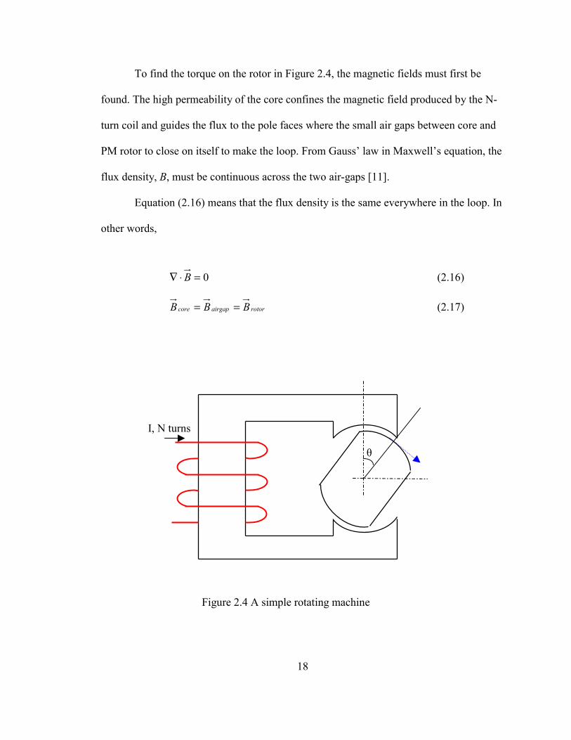
To find the torque on the rotor in Figure 2.4, the magnetic fields must first be

found. The high permeability of the core confines the magnetic field produced by the N-

turn coil and guides the flux to the pole faces where the small air gaps between core and

PM rotor to close on itself to make the loop. From Gauss’ law in Maxwell’s equation, the

flux density, B, must be continuous across the two air-gaps [11].

Equation (2.16) means that the flux density is the same everywhere in the loop. In

other words,

0=⋅∇ B (2.16)

rotorairgapcore BBB == (2.17)

Figure 2.4 A simple rotating machine

I, N turns

θ

19

Since the magnetic field intensity*, H, is defined as (2.18) and the permeability, µ,

of the core and rotor have very high permeability (for ideal case, µ is assumed as infinity

in soft magnetic materials [12]), the total magnetic field intensity concentrated on the two

air-gaps is

µµµBBH

ro

== (2.18)

where,

µo = permeability of free space (= 4π×10-7)

µr = relative permeability

thus,

ggo

stator HHH <<=µµ

gHH 2=∴∑ (2.19)

Therefore, using Ampere’s law (2.20), the magnetic field intensity of the air-gap,

Hg, can be represented by input current, I, as

∫ ∫ =⋅=⋅c s

NIsdJldH (2.20)

ggggrotorrotorcorecore lHlHlHlHNI 22 ≅++=

gg l

NIH2

=→ (2.21)

* It is also called just ‘magnetic field’

20

where lg is the length of the air-gap and the depth of air-gap, D, should be sufficiently

larger than lg. Next relate equation (2.21) with the flux linkage, λ,

ggoggs

AHNANBsdBNN µλ ==⋅=Φ= ∫

g

go

lIAN

2

2µ= (2.22)

using (2.14) and (2.15),

g

go

lAN

IL

2

2µλ == (2.23)

θµ

λµ

λλRDNl

ANl

LLIW

o

g

go

gm 2

2

2

222

22==== (2.24)

Faraday’s law in Maxwell’s Equations shows the flux linkage is constant with

time when the coil is short circuited as follows:

01 =−=⋅−=⋅ ∫∫ dtd

NsdB

dtdld

sc

λε (2.25)

Equation (2.25) means that the flux linkage is time-constant. Under constant flux

linkage, the torque equation is given by [13]:

θ

θλ∂

∂−=

),(mWT (2.26)*

* for constant current condition,

21

therefore,

22

2

θµλ

θ RDNlW

To

gm =∂

∂−= (2.27)

Using (2.22) to substitute for λ,

g

o

lRDINT

4

22µ= (2.28)

In this section we found that the torque of electric machine can be obtained from

its magnetic field energy. In other words, if we can compute the energy of an electric

machine, we can also calculate the machine torque and winding inductance. Based on this

energy-torque relationship, we can calculate a machine torque using Finite Element

Analysis (FEA).

2.4 Finite Element Analysis – Maxwell 3D

Obtaining the correct value of flux density and magnetic field remains an

important issue for designing an electric machine in verifying the magnetic flux loop and

checking the saturation of flux density in each part of the machine. For this purpose,

FEA is used extensively for the design and performance prediction of all types of electric

machines. It is a numerical technique based on the determination of the distribution of the

22

electric or magnetic fields inside the machine structure, by means of the solution of

Maxwell’s equations. FEA could answer the value of torque or force, winding

inductances, field distributions, back-emf waveforms, demagnetization withstand of

magnets, etc [15].

To present electric or magnetic fields over a large, irregularly shaped region, each

region of the modeled machine is divided into many hexahedral or tetrahedral elements.*

The collection of elements is referred to as the finite element mesh.

In FEA computation, the value of a vector field at a location within an element is

interpolated from its nodal value of the field. For magnetic field calculation, Maxwell 3D

solver divides the H-field into a homogeneous and a particular solution. The solver stores

a scalar potential at each node for the homogeneous solution of magnetic field density, H,

and stores the components of H that are tangential to the element edges [14]. Thus, to

obtain a precise description of the field, each element of the model is small enough for

the field to be adequately interpolated from the nodal values.

However, there is a trade-off between the number of the elements and the amount

of computing resources required for the computation. The accuracy of the solution also

depends on how small each of the individual elements is. Thus, a user should choose an

adequate mesh size for fitting his computer capability.

The computing procedure is as follows. First, the current density, J, is calculated

by input current condition. Using Ohm’s law (2.29), the J of all elements in the model is

obtained and stored.

* Maxwell 3D uses tetrahedral elements.

23

VEJ ∇−== σσ (2.29)

where,

E is the electric field

σ is the conductivity of the material

V is the electric potential

Under steady state conditions, the charge density, ρ, in any region of the model

does not change with time [14]. That is

0=∂∂=⋅∇

tJ ρ (2.30)

Substituting (2.29) into (2.30):

( ) 0=∇⋅∇ Vσ (2.31)

The differential equation (2.31) is solved to get the J for all elements. After

computing the current density, the FEA solver computes the magnetic field using

Ampere’s law and Maxwell’s equation describing the continuity of flux,

JH =×∇ (2.32)

0=⋅∇ B (2.33)

Next, the energy is calculated. In a linear material, the energy, W, is the same as

its coenergy, Wc, as

24

( ) dvHBdvHBdWvv∫∫ ⋅=⋅=

21 (2.34)

( ) WdvHBdvHdBWvv

c =⋅=⋅= ∫∫ 21 (2.35)

However, in a nonlinear material, the coenergy is different from its energy like

shown in Figure 2.5. Energy and coenergy in the figure indicate the area above and below

the B-H curve.

If the motion of a material has occurred under constant current conditions (steady-

state), the mechanical work done can be represented by increasing its coenergy [13]. FEA

solver is computing H under constant input current condition, thus, it uses

coenergy differentiation over a given angle instead of energy differentiation for torque

calculation with nonlinear data of the materials.

(a) Linear material (b) Nonlinear material - µ is constant - µ is not constant - energy is equal to coenergy - energy is less than coenergy

Figure 2.5 Comparing B-H curve between linear and nonlinear material

B B

H H

Energy Energy

Coenergy

Coenergy

25

θddWT c= (2.36)

Computing inductance of conductors from the flux linkage is an additional

function of FEA, and these calculated inductance values can be used for dynamic analysis

of the designed machine combined with its controller circuits.

2.5 Summary

This chapter describes the basic theories analyzing the generating torque in

IPMSM for steady-state; using phasor diagrams. Equations (2.10) and (2.12) present that

IPMSM has two torque components: permanent magnet torque and reluctance torque. By

the existence of reluctance torque, the torque of IPMSM is not linearly proportional to the

stator phase current amplitude.

Therefore, FEA is an effective method to predict the value of output torque of

IPMSM. This chapter introduces how the energy of a machine can convert to its output

torque; and then shows the basic theories about FEA for calculation of machine torque.

26

CHAPTER 3

FEA Simulation of the Concept of a New IPMSM

3.1 Introduction

The basic idea is simple; use DC excitation current to control air-gap flux.

Conventional electric machines are constructed from the following parts: a rotor

assembly, laminated stator material, phase current-carrying conductors, and a physical

structure to support the entire machine. When a current-carrying conductor is placed in a

magnetic field from the rotor, the conductor experiences a mechanical force or torque.

This force or torque is directly proportional to the intensity of the magnetic field. Thus,

generating a magnetic field from permanent magnets enables a machine to have high

power density and efficiency. However, the fixed magnetic field limits its field

weakening capability for wide constant power operation.

If a controllable magnetic field can be added to the field of a permanent magnet,

we can vary the field intensity while still maintaining the advantages of PM machines.

DC current is a good source for this purpose, because it is easily increased and decreased.

Moreover, the flux generated by DC current is linearly proportional to the amount of the

current flow until it reaches the saturation region of the flux-carrying material.

FEA is a useful method to check this idea. A simple model is constructed for trial

simulation, and the results are used for the actual design.

27

3.2 Modeling

Figure 3.1 shows the basic model which needs to increase air gap flux. The

permanent magnet used in this model is a ferrite magnet of which the residual flux

density, Br, is 0.4 T and the relative permeability, µr, is 0.25. The steel is a kind of cast

steel of which the µr is about 900 in the linear region.

The flux from the left side of the PM travels through the left upper core, air gap,

top core, air gap again, right upper core, and then returns to the right side of PM. After

FEA simulation, the calculated air-gap flux density of this simple model is about 0.28 T

(Figure 3.2). The object is to increase this air-gap flux density by DC excitation current.

Figure 3.1 Simulation concept model to increase air gap flux

Top Core

Lower Core

Right Upper Core

Air gap

Left Upper Core

28

Figure 3.2 FEA simulation result of air-gap flux density of the concept model

To use excitation current, an additional flux path is needed. For this purpose, two

side cores are attached to the original model as shown in Figure 3.3. Each side core is

directly contacted with half of the top core and makes another air-gap (side air-gap) with

an upper core on both sides. The reason to make the side air-gap between side core and

upper core is that the upper cores are considered as parts of rotor assembly for the

rotating machine. Two coils are wound on each side core to carry DC excitation current.

The direction of the flux from excitation current is perpendicular to that from PM,

and the two fluxes will be combined in the main air-gap between the upper core and the

top core. Actually, there are several methods to attach a side core, but the arrangement in

Z

F

X

Y

29

igure 3.3 Simulation model with side cores and

current direction

wound coils

side air-gap

excitation flux path

30

Figure 3.3 is the best position from the results of FEA simulations about various

configurations.

3.3 Numerical Analysis

Assume that the excited flux from each side core flows through just one half of

the top core with the x-axis direction in Figure 3.3. Then, the new flux path for excitation

current can be simplified as Figure 3.4. The dimensions of the simulation model are

indicated in Figure 3.4. The depth of each part is 40 mm for side core, 50 mm for top

core, and 45 mm for upper core. Suppose that the flux flows only at the center of each

core and air-gap, then the path can be divided with 7 parts: 1, 2*, 3, 4, 5, g1, and g2.

For each part of the path, the length and cross-sectional area are

l1 = 144 mm

l2 = 50 mm

l3 = 30 mm

l4 = 10 mm

l5 = 50 mm

lg1 = lg2 = 2 mm

* For this part, assume that the flux flows in only the top portion of the top core.

31

Figure 3.4 Simplified model for excited flux path

A1 = 20×40 = 800 mm2

A2 = 20×50 = 1000 mm2

A3 = 100×50 = 5000 mm2

A4 = 100×45 = 4500 mm2

Ag1 = 100×50 = 5000 mm2

Ag2 = 20×45 = 900 mm2

Since the reluctance of the magnetic path is defined as

AlR

ro µµ= (3.1)

I

60 100

40

20

2

2

22

l1 l2

l3

lg1

l4 l5 lg2Side core

Top core

Upper core

32

and the relative permeability of the core is 900, the total reluctance is

567

3

1 1059.110800900104

10144 ×=××××

×= −−

−

πR [At/Wb]

52 10442.0 ×=R [At/Wb]

53 10052.0 ×=R [At/Wb]

54 10020.0 ×=R [At/Wb]

55 10491.0 ×=R [At/Wb]

51 1018.3 ×=gR [At/Wb]

52 1068.17 ×=gR [At/Wb]

51046.23 ×≅= ∑ RRtotal [At/Wb]

If the input current is 1000 At, then the flux and main air-gap flux density are

45 1026.4

1046.231000 −×≅

×==Φ

RNI [Wb]

09.010500

10.46

4

≅×

×=Φ= −

−

gg A

B [T]

Therefore, we can expect that the main air-gap flux density reaches about 0.37 T

with the PM.

33

3.4 Simulation Results

FEA simulations have been conducted under four different input current

conditions: 1000 At, 500 At, 0 At, and -500 At. The negative value means that the current

flows the reverse way and the direction of excited flux also changes.

The calculated values of the main air-gap flux density are shown in Figure 3.5.

The value at 1000 At is about 0.35 T and is a little lower than the expected value, 0.37 T.

The reason is that the additional flux path, side core, increases the total reluctance, and

then decreases the flux from the PM in the air-gap. The simulation result also shows that

the flux density is about 0.26 T with side core and no current, and this value is lower by

about 0.02 T than the result without side core. Considering this situation, the main air-gap

flux density increases about 0.09 T. This result totally agrees with the numerical analysis.

Additionally, Figure 3.5 shows that the main air-gap flux density could be greatly

reduced by changing the DC current direction. Comparing Figure 3.6 (a) and (b), the flux

in the side core changes its direction and the air-gap flux is reduced. The arrows in the

air-gap hold their direction but the size of the arrows is shrunk.

This chapter validates the effectiveness of the design concept for a new IPMSM.

As a consequence of the results of the simulations in this chapter, DC excitation current

can be used for increasing and controlling air-gap flux of the electric machine. However,

constructing an adequate flux path for the excited flux is a difficult task in the actual

machine design. An inadequate flux path can increase the total reluctance of PM and the

leakage flux of the machine.

34

Figure 3.5 Simulation results of air-gap flux density for different excitation conditions

35

(a) Excitation current source is 1000 At

(b) Excitation current source -500 At

Figure 3.6 B vector on three cut-planes in the simulation model

Positive air-gap B vector on each cut-plane

36

CHAPTER 4

Design a New Concept Motor

4.1 Design Procedure

As mentioned in the previous chapter, the objective of this research is to design an

electric machine which has high torque density and has controllable air-gap flux directly

for the application of HEV systems. For this purpose, the design procedure is as follows:

1) analysis of pre-developed machine by FEA

- without DC excitation parts

- calculating output torque and air-gap flux density

2) analysis of draft-design machine by FEA

- attaching DC excitation parts

- checking flux saturation and leakage parts

3) fixing design parameters of the new machine by FEA

- reforming flux saturation and leakage parts

- comparing output torque and air-gap flux density with the results of

the pre-developed machine

37

4.2 Pre-developed Motor

4.2.1 Geometries and materials of pre-developed motor

Figure 4.1 shows a quarter part of a pre-developed motor which has been

designed at National Transportation Research Center of Oak Ridge National Laboratory.

The dimensions of the stator and rotor are given in Table 4.1. This IPMSM is a three-

phase and eight-pole (four-pole pair) machine which means that the number of stator

slots per pole per phase is 2. The winding pattern is a single-layer winding with 9 turns

and the winding span is full-pitch as shown in Figure 4.1.

The permanent magnet material used in this motor is ferrite of which remanence

flux density (Br) is 0.4 T, coercive field (Hc) is 1273240 A/m, and relative permeability

(µr) is 0.25. The location of the PM in the rotor is indicated in Figure 4.2.

Laminated silicon steel is used for stator and rotor core to reduce hysteresis and

eddy current loss, and the shaft is made of mild-steel. These two materials have a non-

linear magnetic characteristic, which is shown in Figure 4.3.

Table 4.1 Specifications of stator and rotor

parameters value parameters value

Number of stator slots 48 Air-gap length 0.029 in

Outer stator diameter 10. 6 in Outer rotor diameter 6.317 in

Inner stator diameter 6.375 in Inner rotor diameter 3.3125 in

Stator tooth width 0.349 in Rotor rib thickness 0.05 in

Slot opening width 0.076 in Rotor axial length 2.75 in

Stator axial length 2.5 in PM thickness 0.25 in

38

Figure 4.1 A quarter model of pre-develope

d-axis

q-axis

b

b

b

rotor

PMshaft

N N

N

S

S

S

a

a

c

c

a

a b

d motor for FEA

c

c

stator

39

Figure 4.2 The location of PMs in the rotor

0.505

0.56

1.75

2.05

1.04

22.5°

rotor rib

40

(a) Silicon steel

(b) Mild steel

Figure 4.3 B-H curves for non-linear materials

41

4.2.2 Simulation results of pre-developed motor

The no-load simulation is implemented to check the distribution of the air-gap

flux. Figure 4.4 is a flux density curve for no-load condition along the line which places

on the middle of the air-gap at the center of the rotor in an axial direction. In the figure, it

is observed that the slot openings affect the flux density distribution and the flux wave is

well balanced between north (positive) and south (negative) poles. The average value of

the magnitude of the flux density is 0.1826 T but the effective value coming through the

stator teeth is about 0.3 T as shown in Figure 4.4.

Figure 4.4 Air-gap flux density distribution of pre-developed motor

42

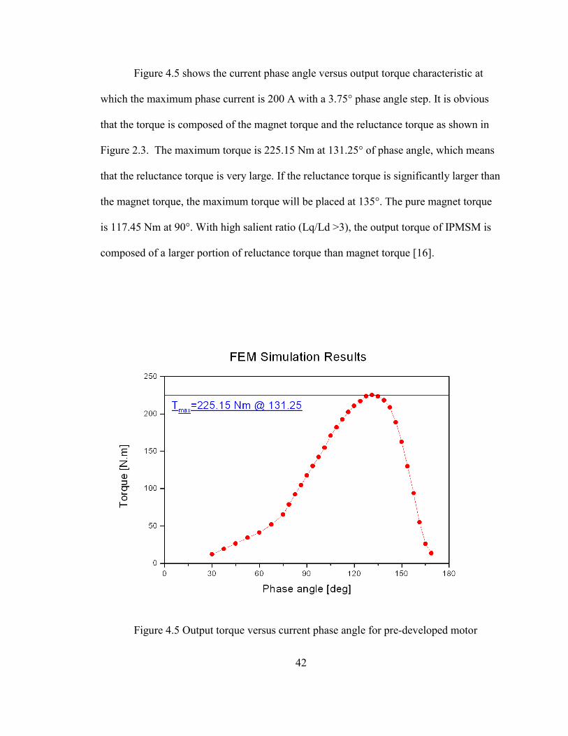
Figure 4.5 shows the current phase angle versus output torque characteristic at

which the maximum phase current is 200 A with a 3.75° phase angle step. It is obvious

that the torque is composed of the magnet torque and the reluctance torque as shown in

Figure 2.3. The maximum torque is 225.15 Nm at 131.25° of phase angle, which means

that the reluctance torque is very large. If the reluctance torque is significantly larger than

the magnet torque, the maximum torque will be placed at 135°. The pure magnet torque

is 117.45 Nm at 90°. With high salient ratio (Lq/Ld >3), the output torque of IPMSM is

composed of a larger portion of reluctance torque than magnet torque [16].

Figure 4.5 Output torque versus current phase angle for pre-developed motor

43

4.3 Embodiment of the Concept

4.3.1 Side-poles and side-magnets

To make a flux path for the excitation current, side-poles are used. These side-

poles are attached to the rotor assembly as shown in Figure 4.6. In the figure, the right

side-pole is arranged to meet the north pole of the PM (N-position), and the left side-

poles are placed to face the south pole of the PM (S-position). Since the side-poles are

made with mild steel and clamped by non-magnetic material (aluminum), the axial-

direction flux can come into or out from the rotor only through the side-poles.

A consequence of FEA has revealed that much leakage flux flows into the rotor

by clamping. To prevent this leakage flux, permanent magnets are used. These magnets

are called side-magnets and placed between side-poles at S-position for right side and at

N-position for left side of the rotor as shown in Figure 4.7. At S-position, they block the

flux from flowing into the rotor through the side-poles because the permanent magnets

are magnetized to have the direction from left to right. Figure 4.8 and Figure 4.9 clearly

shows that the leakage flux is significantly reduced and more flux comes into the rotor

through the side-poles. Correspondingly, the air-gap flux is also increased.

The excitation flux path is indicated in Figure 4.10. The flux generated by DC

excitation current will flow through the frame, flux collector, side air-gap, side-pole, rotor

core, air-gap, and stator. At N-position, the side-poles will attract the axial flux, and then

will send the flux into the rotor. As a result, the air-gap flux will be increased. In contrast,

left side-poles will do the reverse role at S-position. The details will be explained in the

latter part of this section.

44

(a)

(b) left view of rotor assembly (c) right view of rotor assembly (Two side- poles place at S-position) (One side-pole places at N-position)

Figure 4.6 Configuration of side-poles

Rotor assemblyMetal binding

Side-pole

Clamping

Side-pole

Side-pole

S

S S N

45

(a)

(b) left view of rotor assembly (c) right view of rotor assembly (Two side- poles place at S-position) (One side-pole places at N-position)

Figure 4.7 Configuration of side-poles and side-magnets

S

S

S

Side-pole

Side-magnet

Side-magnetsSide-magnet

Side-poles

46

(a) with side-pole only

(b) with side-pole and side-magnet

Figure 4.8 Flux density vector distributions around side-pole at centered N-position

Side-pole

Side-pole

Rotor

Leakage flux

Leakage flux

Side-magnet

S N

47

(a) with side-pole only

(b) with side-pole and side-magnet

Figure 4.9 Magnitude of the flux density on the side-pole and the clamping at centered

N-position

(

(

PM flux

Excitation flux w

Figure 4

Frame

Side-magnet

Excitation coils

Stator

Flux collector S N

Side-pole

N

a) N-position

b)

it

.10

S Side-pole

PM Shaft

S N

Side-magnet

S

48

S-position

Excitation flux with side-pole

hout side-pole penetrating flux

Axial flux path of the motor

N

49

4.3.2 Excitation flux paths

Figure 4.10 shows how the excitation flux flows inside the motor. Figure 4.10 (a)

is the axial cut plane at the N-position, and (b) is the plane at the S-position. For N-

position, the excitation flux from the right side in the Figure 4.10 (a) combines with the

main PM flux in the air-gap, whereas the excitation flux from left side changes its way to

the radial direction along the stator and combines at the flux collector. In the same way,

the excitation flux makes its path for S-position as shown in Figure 4.10 (b). There

should also be some penetrating flux which flows along the outer surface of the stator and

shaft.

Figure 4.11 and Figure 4.12 are the simulation results showing that the excitation

flux flows along the same way as the concept in Figure 4.10. On the left side in Figure

4.11 and the right side of Figure 4.12, the flux density vectors make an independent open

path separated from the main closed path. Therefore, the flux on the open path should go

out and come in from the radial direction.

4.3.3 Excitation coil resistance

If the excitation coils absorb much real power, the operating temperature will be

significantly increased, and the efficiency of the motor will be also decreased. Therefore,

it is necessary to ensure the low resistance of the excitation coils. Resistance in general is

given by the following expression

c

c

Al

R⋅

=ρ

(4.1)

50

Figure 4.11 Flux density vector distributions on the axial cut plane at N-position

Figure 4.12 Flux density vector distributions on the axial cut plane at S-position

51

where lc is the conductor length, Ac is the cross sectional area of the conductor, and ρ is

the conductor resistivity. For most conductors, including copper, resistivity is a function

of temperature that can be linearly approximated as

( )[ ]1212 1)()( TTTT −+= βρρ (4.2)

where ρ(T) is the resistivity at a temperature T and β is the temperature coefficient of

resistivity. For annealed copper commonly used in motor windings, ρ(20°C) =1.7241×10-

8 Ωm, and β =4.3×10-3 °C -1[17]. Suppose that the excitation coil temperature increases

up to 100 °C, then the resistivity of the excitation coils is

( )[ ]( )[ ]

]m[103172.220100103.41107241.1

201001)20()100(

8

38

Ω×=−×+×=

−+=

−

−−

CCCC βρρ

For the space of the excitation current, suppose that the axial height of each frame

is increased 0.5 inches, then the additional space, Aspace

056.15.02

375.66.105.02

,, =×−=×−

= insoutsspace

DDA [in2]

where Ds,out and Ds,in are stator outer diameter and inner diameter respectively. With the

coil packing factor 0.5, the total space allowed for the excitation coils is

528.05.0 == spaceexc AA [in2] 6.340≅ [mm2]

52

The above result means that the excitation coils can be composed of 1mm2 coils

with 300 turns. The length of excitation coils can be calculated with the average value of

the outer and inner stator diameters.

( ) ( ) 6.15998300375.66.10300,, =×+=×−= ππ insoutsexc DDl [in]

4.406≅ [m]

thus, the resistance value of the excitation coils is

417.9101

4.406103172.2)100(6

8

=×

××=⋅

= −

−

exc

excexc A

lCRρ

[Ω]

When the maximum excitation current is 10 A, the power loss from both sides of

the excitation coils is

1883417.91022 22, =⋅×=⋅×= excDCexcloss RIP [W]

For a high power motor (over 50 kW), the power loss is less than 4 % of its output

power. Considering that the motor needs not to be always operating at the maximum

output and the output power can be controlled by the excitation current, the power loss is

not severe.

53

4.4 Simulation Results of Final Model

After conducting several simulations, the model is modified by eliminating the

saturation part of the machine. Also, the inner diameters of side-poles, side-magnets, and

flux-collector are decreased to reduce the leakage flux in the axial direction.

4.4.1 Air-gap flux

To check the relationship between the excitation current and air-gap flux, FEA

simulations have been conducted under several different excitation current values: 3000

At, 2000 At, 1000 At, 0 At, and -1500 At. The simulation results are shown in Figure

4.13. Under positive excitation current, there is a little unbalance between positive and

negative main curves. It may be due to the leakage flux that penetrates the rotor and

stator in the axial direction.

Comparing Figure 4.4, the air-gap flux density significantly increases when the

excitation current is 3000 At (from 0.1826 T to 0.4798 T in average value). Additionally,

Figure 4.13 shows that the air-gap flux density is reduced by decreasing the excitation

current value without changing its own shape.

When the negative excitation current is less than -1500 At, the magnitude of the

flux density is almost the same as when -1500 At, but it loses its own shape. Considering

that the fundamental component of the air-gap flux is mainly related with the motor

performance, it is meaningless to compare between the values when less than -1500 At

and others.

54

Figure 4.13 Simulation results of air-gap flux density for different excitation values

55

With -1500 At of excitation current, the air-gap flux can be weakened by about

6.5% of the maximum value. In other words, the maximum speed of the motor can be 15

times its base speed by just controlling its dc excitation current, if the entire field crossing

the phase conducts is dependent on this air-gap flux.

Figure 4.14 is the flux density vector distributions in the stator and rotor at no

phase current with excitation current of 3000 At, and Figure 4.15 is the magnitude of flux

density in the same condition with Figure 4.14.

Figure 4.16 shows the flux density vectors in the stator and rotor at the maximum

torque position (123.75 ° ) under the maximum phase current of 200 A and excitation

current of 3000 At. The corresponding magnitude of flux density distribution is shown in

Figure 4.17. Both figures (Figure 4.16 and Figure 4.17) present that the flux lines are well

balanced and there is no saturation part in the stator and rotor except rotor ribs. (Stator

and rotor is saturated at about 1.8 T as indicated in Figure 4.3.)

Although the flux flowing through the rotor ribs is also a leakage flux which

remains inside rotor without crossing the air-gap, the ribs are necessary for mechanical

reason: to maintain laminated rotor core shape. In normal condition, the ribs cannot avoid

to be saturated [18].

Figure 4.18 is the overall magnitude of the flux density with the maximum phase

current of 200 A and excitation current of 3000 At. The circumferential area of side-poles

is saturated as shown in the figure. That means the excitation flux is concentrated at the

side-pole from the frame which is the main path of the excitation flux.

56

Figure 4.14 Flux density vector distributions at no phase current (Iexc=3000At)

Figure 4.15 Magnitude of flux density at no phase current (Iexc=3000At)

57

Figure 4.16 Flux density vector distributions at maximum torque position

(Iph,max= 200A, Iexc=3000At)

Figure 4.17 Magnitude of flux density at maximum torque position (Iph,max= 200A, Iexc=3000At)

58

Figure 4.18 Overall magnitude of flux density at maximum torque position (Iph,max= 200A, Iexc=3000At)

59

4.4.2 Output torque

Figure 4.19 shows the current phase angle versus output torque characteristic at

which the maximum phase current is 200 A and the excitation current is 3000 At. In the

figure, the results are compared with those of the pre-developed motor before attaching

the excitation magnetic circuit.

The maximum torque is increased from 225.15 Nm to 283.06 Nm (25.7 %

increase). Since the excitation current increases the air-gap flux, the magnet torque is also

increased; and then, the maximum torque position is shifted slightly from 131.25°

to116.25°. Table 4.2 presents the output torque results along the various excitation

current values; Figure 4.20 is the graph of Table 4.2.

Figure 4.19 Comparison of output torque between pre-developed and final model

60

Table 4.2 Calculated output torque under various excitation current values [Nm]

Phase Angle

3000 At 2000 At 1000 At 0 At -1500 At

90° 207.08 187.33 124.99 90.93 63.87 93.75° 219.49 195.99 131.93 101.28 79.09 97.5° 231.49 203.33 139.71 110.65 90.53 101.25° 242.21 208.44 147.24 115.24 101.44 105° 253.05 214.87 154.06 124.87 110.16 108.75° 267.97 228.06 167.42 135.00 124.73 112.5° 276.78 235.03 170.49 147.33 132.49 116.25° 283.06 239.24 177.2 154.78 141.81 120° 282.99 245.04 181.56 162.04 150.24 123.75° 281.99 249.77 186.02 168.14 156.63 127.5° 278.78 238.26 189.89 173.71 160.00 131.25° 271.98 228.01 187.06 174.81 161.31 135° 263.53 222.65 184.11 174.16 160.93

Figure 4.20 Comparison of output torque under various excitation current values

61

4.5 Summary and Discussion

FEA simulations have been conducted for a newly designed PM machine that

attaches excitation coils and excitation flux path to the target model which is described in

Section 4.2. The results of the simulations clearly show the outstanding characteristic of

the newly designed motor as compared to that of the pre-developed motor. The maximum

torque increases 225.15 Nm to 283.06 Nm (25.7 % increase).

The simulations have also confirmed that the air-gap flux can be changed by the

excitation current value. Under 3000 At, the average of the air-gap flux density is

0.4798 T, which is about 15.3 times of the value under -1500 At (0.0313 T).

The pure PM torque can be obtained from Table 4.2 at 90° phase angle,

207.08 Nm under 3000 At and 63.87 Nm under -1500 At. Since the PM torque is directly

proportional to the air-gap flux*, the pure PM torque of -1500 At is too large considering

its air-gap flux density. When -1500 At, the calculated torque value is about 30.8 % of

the value in case of 3000 At, but the air-gap flux is only 6.5 %.

A comparison between the pre-developed motor and the final model with 0 At of

excitation current reveals that there is a big difference in the air-gap flux density (0.1826

T for the pre-developed motor and 0.1347 T for 0 At) since the excitation flux paths can

increase the total reluctance of the motor. Correspondingly, the calculated PM torque in

both cases is clearly different (117.45 Nm for the pre-developed motor and 90.93 Nm for

0 At). However, the percentage of the pure PM torque is similar that of the air-gap flux

density (77.4 % for torque and 73.8 % for flux density) because the air-gap flux and the

* T=KT·I, and KT ∞ Φ

62

flux linkage of the phase conductors come from only PMs when the excitation current is

0 At.

Therefore there must be other magnetic fields which cross the phase conductors

without passing the air-gap. Table 4.3 indicates PM torque and air-gap flux density ratios

of each excitation current to the excitation current of 0 At. When the excitation current is

positive, the torque ratio is much less than the flux density ratio; and when negative, the

torque ratio is greater than the flux density ratio. These results suggest that positive

excitation current decrease the flux linkage crossing the phase conductors and negative

excitation current increase that.

Comparing Figure 4.21 (positive excitation current, Iexc=3000At) with Figure 4.22

(no excitation current), the flux density in the stator teeth is not uniformly distributed

along the axial direction. At N-position in Figure 4.21, the flux density is counter-

balanced in the middle of the left part of stator teeth, and at S-position, the right part. As

a consequence, the effective flux crossing the phase conductor will be reduced. With

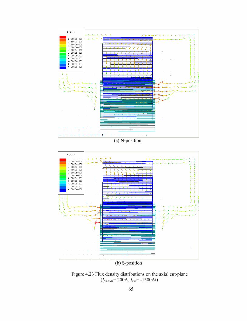
negative excitation current, the flux density vectors change their direction in the air-gap

(Figure 4.23, Iexc= -1500At). That means the air-gap flux in the radial direction will be

Table 4.3 Comparing PM torque and air-gap flux density in each excitation current

Excitation current

PM torque [Nm] ratio Average air-gap flux

density[T] ratio

3000 At 207.08 2.278 0.4798 3.562 2000 At 187.33 2.06 0.4250 3.155 1000 At 124.99 1.375 0.2866 2.128

0 At 90.93 1 0.1347 1 -1500 At 63.87 0.702 0.0313 0.232

63

(a) N-position

(b) S-position Figure 4.21 Flux density distributions on the axial cut-plane (Iph,max= 200A, Iexc=3000At)

64

(a) N-position

(b) S-position Figure 4.22 Flux density distributions on the axial cut-plane (Iph,max= 200A, Iexc=0At)

65

(a) N-position

(b) S-position Figure 4.23 Flux density distributions on the axial cut-plane (Iph,max= 200A, Iexc= -1500At)

66

much smaller than the actual effective flux linkage of phase conductors. To find out the

exact relation between excitation current and effective crossing flux linkage, additional

research works are needed.

For IPMSM, the speed is in inverse proportion to the PM torque or effective flux

crossing the phase conductors [19]. Therefore, the new machine can increase its speed

about 3.24 times of its base speed without control of the direct and quadrature axis

current components.

67

CHAPTER 5

Conclusions and Future Works

5.1 Conclusions

Permanent magnet motors are desirable for applications that require high power

density such as EV and HEV. However, they have critical disadvantages; the high price

of high-energy permanent magnet and the complexity of the controller for field

weakening if it is necessary to drive them at a constant power output above the base

speed.

To solve these undesirable properties of IPMSM, a new type of IPMSM structure

is developed and analyzed in this thesis. The new motor has excitation coils and

additional magnetic paths for the excitation flux which can increase the air-gap flux as

well as the output torque. Additionally, the new motor may have the performance that its

air-gap flux (effective flux) can be controlled directly through the magnitude and

direction of its DC excitation current. The permanent magnets used in the new motor are

Ferrite which are much cheaper than high energy PM materials (Samarium Cobalt and

Neodymium Iron Boron).

The FEA simulation works were shown, and the results presented that the

excitation current can be used for controlling the output torque as well as air-gap flux.

Maximum output torque is increased by about 25.7% compared with the simulation result

of the motor without excitation coils and paths.

68

However, the discordance between PM torque and air-gap flux may be caused by

the excitation current which reduces or increases the effective flux linkage of the phase

conductors. Therefore, additional research must be conducted to find the exact relation

between excitation current and effective winding flux linkage.

The new motor is designed for the purpose of the applications of EV or HEV. The

maximum torque (283.06 Nm) shows the possibility of the application of vehicles from

the point of view of output torque compared to the motor used for commercial HEV*.

The commercial motor has the maximum torque of about 350 Nm with 3.5 inches axial

stator and rotor length [20]. Considering the possibility of increasing torque with higher

excitation current, this research suggests a new design concept of IPMSM which has

similar or higher power density than the commercial motor. Moreover, the new motor

makes use of Ferrite as its permanent magnet, not Rare Earth or Samarium Cobalt.

In the respects mentioned above, the new motor has several advantages. Firstly,

the manufacturing cost will be significantly reduced by low price of magnets and short

length of stator and rotor core. Secondly, the inertia of rotor will be reduced, and it will

allow the motor to have a fast response to load variations. Lastly, the direct controllability

of air-gap flux will allow the motor to be operated easily above its base speed. On the

other hand, the existence of side air-gap is the main disadvantage of the new motor

because it can make the axial vibration or unexpected torque ripple.

* Toyota’s Prius

69

5.2 Future Works

For the confirmation of this research works and better characteristics of the motor,

following research works should be conducted.

• Improving the motor characteristics to have wider speed range by

controlling DC excitation current.

• Clarification of the reasons for the discordance between PM torque and

air-gap flux.

• Expectation of dynamic behavior including the effect of side air-gap.

• Analysis of the saturation effect on the rotor and the excitation flux paths,

and then adjusting the geometric dimensions.

• The possibility of irreversible demagnetization of Ferrite magnet.

• Developing new control strategy including the excitation current variable.

• Thermal analysis of the motor including the excitation coils to get more

reliable results.

• Cost analysis

• Building a prototype sample and testing to prove the results of this

research and predict the machine behavior.

70

REFERENCES

71

References

[1] I. Boldea, L. Tutelea, and C. I. Pitic, “PM-assisted reluctance synchronous

motor/generator (PM-RSM) for mild hybrid vehicles: electromagnetic design,” IEEE

Transactions on Industry Applications, vol. 40, no. 2, March-April 2004,

pp. 492 – 498.

[2] M. Ehsani, G. Yimin, and S. Gay, “Characterization of electric motor drives for

traction applications,” Industrial Electronics Society, 2003. IECON '03. The 29th Annual

Conference of the IEEE, vol. 1, Nov. 2003, pp. 891 – 896.

[3] Z. Rahman, K. L. Butler, and M. Ehsani, “Effect of extended-speed, constant-power

operation of electric drives on the design and performance of EV propulsion system,”

SAE Future Car Congress, Apr. 2000, Paper No. 2001-01-0699.

[4] J. S. Lawler, J. M. Bailey, and J. Pinto, “Limitations of the conventional phase

advance method for constant power operation of the brushless DC motor,” IEEE

Proceedings Southeast Con., April 2002, pp. 174-180.

[5] T. J. E. Miller, Brushless Permanent-Magnet and Reluctance Motor Drive, London,

U.K., Clarendon Press, 1989.

[6] D. A. Staton, W. L. Soong, and T. J. E. Miller, “Unified theory of torque production

in switched reluctance and synchronous reluctance motors,” IEEE Transactions on

Industry Applications, vol. 31, no. 2, March/April 1995, pp. 329 – 337.

[7] S. Morimoto, M. Sanada, and Y. Takeda, “Performance of PM-assisted synchronous

reluctance motor for high-efficiency and wide constant-power operation,” IEEE

Transactions on Industry Applications, vol. 37, no. 5, Sept./Oct. 2001, pp. 1234 – 1240.

72

[8] S. Morimoto, M. Sanada, and Y. Takeda, “Performance of PM/reluctance hybrid

motor with multiple flux-barrier,” Proceedings of the Power Conversion Conference -

Nagaoka 1997, vol. 2, 3-6 Aug. 1997, pp. 649 – 654.

[9] S. Kawano, H. Murakami, N. Nishiyama, Y. Ikkai, Y. Honda, and T. Higaki, “High

performance design of an interior permanent magnet synchronous reluctance motor for

electric vehicles,” Proceedings of the Power Conversion Conference - Nagaoka 1997,

vol. 2, 3-6 Aug. 1997, pp. 33-36.

[10] D. Jones, “A new buried magnet brushless PM motor for a traction application,”

Proceedings of the Power Conversion Conference - Nagaoka 1997, vol. 2, 3-6 Aug.

1997, pp. 33-36.

[11] C. R. Paul, K. W. Whites, and S. A. Nasar, Introduction to Electromagnetic Fields,

Massachusetts, U.S., WCB/McGraw-Hill, 1998.

[12] J. Chiasson, Modeling and High Performance Control of Electric machines, U.S.,

John Wiley & Sons, 2005.

[13] P. C. Sen, Principles of Electric Machines and Power Electronics, 2nd, NewYork,

U.S., John Wiley & Sons, 1997.

[14] “Maxwell 3D v.10, Online Help Manual,” Ansoft Corp., 2004, pp. 692-754.

[15] Z. Q. Zhu, G. W. Jewell, and D. Howe, “Finite element analysis in the design of

permanent magnet machines,” IEE Seminar on Current Trends in the Use of Finite

Elements (FE) in Electromechanical Design and Analysis (Ref. No. 2000/013), Jan. 2000,

pp. 1/1 - 1/7.

73

[16] K. Sakai, T. Hattri, N. Takashi, M. Arata, and T. Tajima, “High efficiency and high

performance motor for energy saving in systems,” IEEE Power Engineering Society

Winter Meeting 2001, vol. 3, Jan./Feb. 2001, pp. 1413 – 1418.

[17] D. C. Hanselman, Brushless Permanent-Magnet Motor Design, NewYork, U.S.,

McGraw-Hill, 1994

[18] J. H. Lee, J. C. Kim, and D. S. Hyun, “Effect analysis of magnet on Ld and Lq

inductance of permanent magnet assisted synchronous reluctance motor using finite

element method”, IEEE Transaction on Magnetics, vol. 35, no. 3, May 1999, pp. 1199-

1202.

[19] B. Bae and S. Sul, “Practical design criteria of interior permanent magnet

synchronous motor for 42V integrated Starter-Generator,” IEEE International Electric

Machines and Drives Conference 2003, vol. 2, June 2003, pp. 656-662.

[20] C. W. Ayers, J. S. Hsu, L. D. Marlino, C. W. Miller, G. W. Ott, Jr., and C. B. Oland,

“Evaluation of 2004 Toyota Prius Hybrid Electric Drive System Interim Report,”

Tennessee, U.S., Oak Ridge National Laboratory, Nov. 2004, Report No. ORNL/TM-

2004/247

74

APPENDICIES

75

Appendix A

Flowchart of Maxwell 3D

START

Drawing Model

Input Material Data

Input Current & Boundary Conditions

Error exists?

Check Modeling Error

Generating Initial Mesh

Start Solution Process

Solve for conduction current (J)

Write solution files

Perform error analysis

Solution criterion satisfied?

Solution finished

YES

Perform error analysis

Error criterion satisfied?

Solve for magnetic Field (H)

Refine Mesh

Refine Mesh

YES

YES

NO

NO

NO

76

Appendix B

Park’s transformation and Reference Coordinate systems

The Park’s transformation is used to transform three-phase systems into two-axis

models, which defines the method of a transformation from the three-phase system to a

two-axis model (d and q). For synchronous motors, especially with permanent magnets, a

rotor-oriented coordinate system is more convenient. In the dq-system, the d-axis is along

the magnetization of the rotor while the q-axis lies electrically perpendicular ahead in the

direction of positive rotation.

Figure B.1 shows the structure of the three-phase IPMSM with the reference

angles. The a-, b-, and c-axis are fixed on the stator. d- and q-axis are fixed on the rotor,

which define the synchronous reference frame. Any set of three-phase quantities, e.g. the

flux linkages λa, λb, and λc can be transformed in the synchronous reference frame using

Park’s transformation method as the following equations:

−+−+= )

34cos()

32cos()cos(

32 πϑλπϑλϑλλ mcmbmad ppp (B.1)

−+−+−= )

34sin()

32sin()sin(

32 πϑλπϑλϑλλ mcmbmaq ppp (B.2)

where ϑm is the mechanical angle between the reference a-phase axis and the d-axis, and

p is the number of pole-pair.

77

The inverse transformation is then;

[ ])cos()sin( mqmda pp ϑλϑλλ += (B.3)

−+−= )

32cos()

32sin( πϑλπϑλλ mqmdb pp (B.4)

−+−= )

34cos()

34sin( πϑλπϑλλ mqmdc pp (B.5)

Figure B.1 A quarter IPMSM model for references of

d-axis

q-axis

c

c

b

a

b

N

N

N

S

S

S

b-phase axis

c-phase axis

ϑm

a

a

b

c

c

a

b

the three-phase

a-phase axis

78

VITA

SeongTaek Lee was born in Seoul, Korea. He attended Yonsei University in

Seoul majoring in Mechanical Engineering. After receiving a Bachelor of Science degree,

from 1993 to 2000, he worked at Mando Machinery Corporation as a research engineer in

the development of an electric motor for electric vehicle and electric power steering

system.

In 2000, he began attending the University of Tennessee in Knoxville majoring in

Electrical Engineering for a Bachelor of Science degree and started the Master’s program

at same school. His research interests include design, testing, and control of permanent

magnet electric machines.