Título artículo / Títol article: Hippocampal shape ... · independent component analysis are deﬁned for multivariat e functions with two arguments. A functional linear ... Neuropsychology

Título artículo / Títol article:

Hippocampal shape analysis in Alzheimer’s disease using Functional Data Analysis

Autores / Autors

Irene Epifanio, Noelia Ventura-Campos

Revista:

Statistics in Medicine (2013)

Versión / Versió:

Preprint del autor

Cita bibliográfica / Cita

bibliogràfica (ISO 690):

EPIFANIO, Irene; VENTURA-CAMPOS, Noelia. Hippocampal shape analysis in Alzheimer’s disease using Functional Data Analysis. Statistics in Medicine, 2013.

url Repositori UJI:

http://hdl.handle.net/10234/73306

http://hdl.handle.net/10234/73306

Research Article

Statisticsin Medicine

Received XXXX

(www.interscience.wiley.com) DOI: 10.1002/sim.0000

Hippocampal shape analysis in Alzheimer’sdisease using Functional Data Analysis

Irene Epifanioa∗, Noelia Ventura-Camposb

The hippocampus is one of the first affected regions in Alzheimer’s disease. Left hippocampi of controls, mildcognitive impairment and Alzheimer’s disease patients arerepresented by spherical harmonics. Functional dataanalysis is used in the hippocampal shape analysis. Functional principal component analysis and funcionalindependent component analysis are defined for multivariate functions with two arguments. A functional lineardiscriminant function is also defined. Comparisons with other approaches are carried out. Our functional approachgives promising results, especially in shape classification. Copyright c© 0000 John Wiley & Sons, Ltd.

Keywords: Functional data analysis; Shape analysis; Alzheimer’s disease; Principal component analysis;Independent component analysis; Discriminant analysis

1. Introduction

The early diagnosis of Alzheimer’s disease (AD) is a crucialissue in our society, because the administration of medicinesto individuals who are subtly impaired may render the treatments more effective. Mild cognitive impairment (MCI) isconsidered as a diagnostic entity within the continuum of cognitive decline towards AD in old age [1, 2]. Longitudinalstudies show a direct relation between the hippocampal volume decrease and cognitive decline [3, 4]. However,volumetric measurements are simplistic features and structural changes at specific locations cannot be reflected in them.If morphological changes could be established, then this should enable researchers to gain an increased understandingofthe condition. This is the reason why nowadays shape analysis is of a great importance in neuroimaging [5].

Several shape modeling approaches have been considered in the neuroimaging literature. One of them is the medialrepresentation, where the binary object is represented using a set of atoms and links that connect the atoms together toform a skeletal representation of the object. Styner et al. [6] applied this scheme to hippocampi and other human brainstructures. The distance map approach has been applied in classifying a collection of hippocampi in Golland et al. [7]. Ina distance map, the distance from each point in the image to the boundary of the object is computed. Other approachesinclude deformation fields obtained by warping individual substructures to a template, such as the paper of Joshi et al. [8]applied to the hippocampus, or the landmark approach used with hippocampi by Park et al. [9] or Shen et al. [10]. Insteadof the previous non-parametric models, a parametric approach, which has been successfully applied to model varioussubcortical structures, is the spherical harmonic representation (SPHARM) [11, 12, 13, 14, 15, 16, 17]. Each individualsurface is parameterized by a set of coefficients weighting the basis functions: the spherical harmonics or its weightedversion (the weighted spherical harmonic representation). Styner et al. [5] compared the sampled boundary implied by theSPHARM description with the medial shape description, obtaining good concordance between both descriptions. Otherworks propose global features which discriminate the condition [18]. It is quite common to use some of these approacheswith a principal component analysis for shape classification and group comparison.

The spherical harmonic representation is a particular caseof representing functional data as smooth functions. Thewhole surface is modeled from a set of points belonging to thesurface. Functional data are observed discretely althougha continuous function lies behind these data. In order to convert the discrete observations into a true functional form,each

a Dept. Matematiques, Universitat Jaume I, Campus del Riu Sec, 12071 Castello, Spainb Dept. Psicologia Basica, Clınica i Psicobiologia, Universitat Jaume I, Spain∗Correspondence to: Tel.: +34-964728390, fax: +34-964728429. E-mail: [email protected]

Statist. Med.0000, 001–12 Copyright c© 0000 John Wiley & Sons, Ltd.

Prepared usingsimauth.cls [Version: 2010/03/10 v3.00]

Statisticsin Medicine I. Epifanio and N. Ventura-Campos

function is approximated (smoothed) by a weighted sum (a linear combination) of known basis functions. Functional dataanalysis (FDA) provides statistical procedures for functional observations (a whole function is a datum). The goals ofFDAare basically the same as those of any other branch of statistics. Ramsay and Silverman [19] give an excellent overview.Ferraty and Vieu [20] provide a complementary and very interesting view on nonparametric methods for functional data.A mixture of practical and theoretical aspects is found in Ferraty and Romain [21]. The field of FDA is quite new and thereis still a lot of work to be done, but in recent years several applications have been developed in different fields, especiallyin human health [22, 23, 24].

In Epifanio and Ventura-Campos [25] two-dimensional (2D) shapes were analyzed from the three point of viewsconsidered by Stoyan and Stoyan [26] for describing shapes: firstly, set descriptors; secondly, using landmarks (pointdescription); and thirdly, employing a function describing the contours. The results were compared with these threeapproaches (the set theory approach, the landmark based approach and the functional approach) in two of the mainproblems in form statistics: the study of the main sources ofvariation among the shapes (principal component analysis,PCA), and classification among different classes (discriminant analysis). The analysis of contour functions by FDA gavemore meaningful results in both problems.

In this work, the hippocampus surface is described by multivariate (three) functions with two arguments. In Section2,the methodology is introduced together with our data. We discuss the extension of the PCA to deal with trivariate functionaldata with two arguments. A discriminant function based on independent component analysis (ICA) is defined for indicatingwhere the differences between groups are and what their level of discrimination is. In Section3, the methodology is appliedto the analysis of structural magnetic resonance imaging (sMRI) scans for studying the hippocampal differences among thesubjects of three groups: cognitively normal (CN) subjects, patients with mild cognitive impairment (MCI), and patientswith early Alzheimer’s disease (AD). Comparison with otherworks is carried out. Finally, conclusions and some openproblems are discussed in Section4.

2. Materials and methods

2.1. Brain sMRI scans processing

A total of 28 individuals (12 CN, 6 MCI and 10 AD subjects) are analyzed in this study, whose description is in Table1. All the individuals were recruited from the Neurology Service at La Magdalena Hospital (Castello, Spain) and theNeuropsychology Service at the Universitat Jaume I. All experimental procedures complied with the guidelines of theethical research committee at the Universitat Jaume I. Written informed consent was obtained from every subject ortheir appropriate proxy prior to participation. Selectionfor the participant group was made after careful neurological andneuropsychological assessment. The neuropsychological test battery involved Digit Span, Similarities, Vocabulary, andBlock Design of the WAIS-III; Luria’s Watches test, and Poppelreuters Overlapping Figure test. sMRI were acquired on a1.5T scanner (General Electric). A whole brain high resolution T1-weighted anatomical reference scan was acquired (TE4.2 ms, TR 11.3 ms, FOV 24 cm; matrix = 256×256×124, 1.4 mm-thick coronal images).

Hippocampi were traced manually on contiguous coronal slices (or sections) following the guidelines of Watson et al.[27], and Hasboun et al. [28]. The hippocampus segmentation was done by an expert tracerwith MRicro software, blindedto the clinical data of the study subjects. The segmentationof each hippocampus lasted approximately 40 minutes. Anexample of the left and right hippocampal contour (drawn in white) in a coronal view is shown in Figure1 (a), whilea sagittal view of one of the hippocampus can be seen in Figure1 (b). Images were visually reoriented. The anteriorcommissure–posterior commissure (ACPC) line was identified and the images were then reoriented parallel to it. Theslices were put together using the isosurface function in Matlab, which gives the vertices and faces of the triangle mesh.

2.2. Surface parametrization

In 2D, the contour is a closed planar curve that consists of the elements of the figure boundary. The contour parametrizationby its arc length can be applied to any contour (note that other contour functions have limitations, see Kindratenko [29]for a review of various contour functions).

This method has been extended to represent analogously the surfaces of closed 3D objects. In this case, instead of twoparametric functions with one parameter, three functions with two angular parameters are needed:x(θ, φ), y(θ, φ), z(θ, φ)(see L. Shen and McPeek [15] for a detailed explanation). Specifically, a surface is mapped onto a unit sphere under abijective mapping. However, unlike the 2D case, some practical problems prevent this mapping from being completelystraightforward. In fact, this one-to-one mapping can be obtained from various surface flattening techniques such asconformal mapping [12], semi-isometric mapping [30], area preserving mapping [13, 31] and the deformable surfacealgorithm [32]. Since the conformal mapping tends to introduce huge area distortion, area preserving mapping is widelyused. However, these flattening methods are computationally intensive and not trivial to implement. Here, we use a new

2 www.sim.org Copyrightc© 0000 John Wiley & Sons, Ltd. Statist. Med.0000, 001–12Prepared usingsimauth.cls

I. Epifanio and N. Ventura-Campos


alternative proposed recently in Chung et al. [17] for objects that are close to either star-shape or convex. The mappingis based on the equilibrium state of heat diffusion. The ideais tracing the geodesic path of heat equilibrium state froma heat source (hippocampus in this case) to a heat sink (sphere). As solving an isotropic heat equation in a 3D imagevolume is computationally trivial, this flattening technique is numerically simpler than any other available methods anddoes not require optimizing a cost function. Details about this method can be found in Chung et al. [17], and how it workscan be seen athttp://www.stat.wisc.edu/∼mchung/research/amygdala/. This step although necessary is auxiliar, and anyother method can be used without changing the following analysis. However, the method from Chung et al. [17] has beeneffective with hippocampi, and we will use it.

Once the surface is mapped onto the sphere, the angles serve as coordinates for representing hippocampus surfaces usingbasis functions. Figure2 shows an illustration of the surface flattening process for one hippocampus with that method, andthe surface parameterization using the angles (θ, ϕ). The pointθ = 0 corresponds to the north pole of a unit sphere.

2.3. Representing functions by basis functions

The first step in FDA is the conversion from discrete data to functions by smoothing. Linear combinations of basisfunctions are used for representing functions. We have chosen as basis the spherical harmonics, because they have beenalready used in similar structures with excellent results,furthermore its orthogonality has computational advantages. Otherpossible basis could be the weighted Fourier series [14], spherical splines [33, 34] or spherical wavelets [35, 36], althoughspherical harmonics is the most used basis in this field.

Although complex-valued spherical harmonics could be usedas in Gerig et al. [11] or Shen et al. [13], we have preferredto used real spherical harmonics as in Chung et al. [14, 17], considering that most applications of spherical harmonicsrequire only real-valued spherical functions, and for convenience in setting up a real-valued stochastic model.

A real basis of spherical harmonics is given by (l is the degree andm is the order):

Ylm(θ, ϕ) =

√2N(l,m)cos(mϕ)Pm

l (cosθ) if m > 0N(l,0)P

0l (cosθ) if m = 0√

2N(l,|m|)sin(|m|ϕ)P |m|l (cosθ) if m < 0

(1)

whereN(l,m) =√

2l+14π

(l−m)!(l+m)! andPm

l is the associated Legendre polynomial of orderm defined over the range[−1, 1]:

Pml (x) = (−1)m

2ll!(1− x2)m/2 dl+m

dxl+m (x2 − 1)l.Let S2 be the unit sphere inR3, andf andg ∈ L2(S2). The inner product is defined by

< f, g >=

∫ π

θ=0

∫ 2π

ϕ=0

f(θ, ϕ)g(θ, ϕ)dΩ =

∫

S2

f(θ, ϕ)g(θ, ϕ)dΩ =

∫

S2

fgdΩ (2)

wheredΩ = sin(θ)dϕdθ. With respect to the inner product, the spherical harmonicssatisfy the orthonormal condition:∫

S2 YlmYl′m′dΩ = δll′δmm′ , whereδij is the Kroneker’s delta.The three functions are independently expressed in terms ofthe spherical harmonic as:x(θ, ϕ) =

∑Ll=0

∑lm=−l c

xlmYlm(θ, ϕ), y(θ, ϕ) =

∑Ll=0

∑lm=−l c

ylmYlm(θ, ϕ) and z(θ, ϕ) =

∑Ll=0

∑lm=−l c

zlmYlm(θ, ϕ). L is the

maximal degree of the representation, which determines thedegree to which data are smoothed. As we know the values ofeach function in a sample of points(θi, ϕi)ni=1, the coefficients can be estimated by least squares. In the case ofx(θ, ϕ)(analogously for the other two functions), letx = x(θi, ϕi)ni=1 be the vector of observations,cx the vector containingthe coefficientscxlm andY = Ylm(θi, ϕi)ni=1 the matrix of basis function values at the observation points, thencx =(Y′

Y)−1Y

′x. If the size of the linear equation is extremely large, the coefficients can be also estimated in a least squares

fashion by the iterative residual fitting (IRF) algorithm [14]. Finally, a vector-valued function can be builtF (θ, ϕ) =(x(θ, ϕ), y(θ, ϕ), z(θ, ϕ))′ =

∑Ll=0

∑lm=−l clmYlm(θ, ϕ), whereclm = (cxlm, c

ylm, czlm)′.

As in other works that used SPHARM for simple surfaces, a small L results in an acceptable degree of smoothing forthis kind of subcortical structures. For more complex structures, such as cortical surfaces, a higher degree (for example,52) is necessary for a good representation [14]. After inspecting the representations for different values ofL, L = 15 wasvisually chosen for our hippocampi. Figure2 shows the spherical harmonic representations of a hippocampus surface fordifferentL. Note that ifL is too small, we miss important aspects of the surface, but with largeL we not only fit data butalso noise. Hence there was an inevitable trade-off betweenthese two factors in choosingL = 15. In order to check if theanalysis is robust to the choice of different values ofL, the classification results for different values ofL are shown in thesupplementary material.

Sometimes, a registration or alignment is then carried out.However, in this case it is not necessary as the location wasremoved previously by translating each hippocampus to the same point in such a way that its centroid coincides with thatpoint ((25,25,25) in our case). Note that the centre of the sphere for the surface parametrization is on each hippocampal

Statist. Med.0000, 001–12 Copyright c© 0000 John Wiley & Sons, Ltd. www.sim.org 3Prepared usingsimauth.cls

http://www.stat.wisc.edu/~mchung/research/amygdala/


centroid, as in Chung et al. [17]. Furthermore, all the hippocampi have the same orientation, so no rotation is needed.As size information (hippocampal volume is a usual discriminatory feature) is important, no scaling correction is carriedout. So we analyze the form, which combines the shape and the size information, otherwise scale can be removed bydividing through the centroid’s size at the beginning, as inEpifanio and Ventura-Campos [25]. Here, no further alignmentis necessary, as in Chung et al. [17], since the coordinates ((θ, ϕ)) on two surfaces are corresponding pairs, and thereforethe coefficients match each other. For other kind of the surface parametrization, an alignment could be necessary asexplained in L. Shen and McPeek [15], where landmarks are used for registration.

In this paper the arguments are angles, but when the argumentis time, functions usually exhibit two kind of variation:amplitude and phase variation. The fist one accounts for the size of the shape features in the functions, whereas the secondone refers to the location of the features. In case that we hadphase variation, the algorithm combining registration withprincipal components analysis in Kneip and Ramsay [37] could be used, where decomposition of functional variation intoamplitude and phase partitions is defined.

2.4. Functional discriminant analysis

Linear discriminant analysis can be used with functions, but regularization is necessary to give meaningful results [22,ch. 8]. Recent advances in functional data classification have been reported by various authors. Many of them involvea type of preprocessing (sometimes implicit) of the functional data (see [38] for a comparison of different methods forunivariate functions, and [25] for multivariate functions with one argument). One possible regularization approach is toconcentrate on the first few principal components as in [22, ch. 8], or some other finite-dimensional representation ofthe data, as ICA, which has given better results than PCA and other alternatives in previous literature [25]. So, once thehippocampi are represented in a basis (SPHARM), we can carryout the functional data analysis, beginning with exploringthe hippocampal variability by PCA and ICA, and using them for the discriminant analysis.

2.5. Functional PCA (FPCA)

For studying the main sources of variation among the hippocampi, principal component analysis is used. In order to seehow PCA works in the functional context, let us recall PCA forMultivariate Data Analysis (MDA). Shortly, summationschange into integrations. In MDA, principal components areobtained by solving the eigenequation

Vξ = ρξ, (3)

whereV is the sample variance-covariance matrix,V = (N − 1)−1X

′X, X is the centered data matrix,N is the number

of subjects observed, andX′ indicates the transpose ofX. Moreover,ρ andξ are an eigenvalue and an eigenvector ofV,respectively.

In the functional version of PCA, PCs are replaced by functions. Before analyzing our multivariate functional datawith multiple arguments, let us introduce the functional univariate case. Letx1(t), . . . , xN (t) be the set of univariateobserved functions with one scalar argumentt. The mean function is defined as the average of the functions point-wiseacross replications (x(t) = N−1

∑Ni=1 xi(t)). If data have been centered (the mean function has been subtracted), the

covariance functionv(s,t) is defined analogously byv(s, t) = (N − 1)−1∑N

i=1 xi(s)xi(t). As explained in Ramsay andSilverman [19, Chapter 8], the functional counterpart of equation3 is the following functional eigenequation

∫

v(s, t)ξ(t)dt = ρξ(s), (4)

whereρ is still an eigenvalue, but whereξ(s) is an eigenfunction of the variance-covariance function, rather than aneigenvector. Now, the principal component score corresponding to ξ(s) is computed by using the inner product forfunctions:si =

∫

xi(s)ξ(s)ds. Note that for multivariate data, the indexs is not continuous, but a discrete indexj replacesit: si =

∑

j xijξj .

For solving the eigenequation4, the original functions could be discretized. However, we will work with the coefficientsof the functions expressed as a linear combination of known basis functions. If the basis is orthonormal, FPCA reducesto the standard multivariate PCA of the coefficient array, asexplained in Ramsay and Silverman [19, Sec. 8.4.2], wherecomputational methods for FPCA are reviewed. This reduces the amount of information generated.

With regard to the number of PCs that can be computed, let us note that in the functional context, “variables” nowcorrespond to values oft, and there is no limit to these. Therefore, a maximum ofN – 1 components can be computed.However, if the number of basis functionsM representing the functions is less thanN, M would be the maximum.

2.5.1. FPCA with multiple functions and multiple argumentsLet Fi(θ, ϕ)Ni=1 be the set of observedfunctions. Each Fi consists of three functional data with two arguments representing one hippocampus




((xi(θ, ϕ), yi(θ, ϕ), zi(θ, ϕ)). Three mean functions (x(θ, ϕ), y(θ, ϕ), z(θ, ϕ)) and three covariance functions(vXX((θ, ϕ), (ϑ, φ)), vY Y ((θ, ϕ), (ϑ, φ)), vZZ ((θ, ϕ), (ϑ, φ))) can be computed pointwisely as before for each kindof function, respectively. We can calculate the cross-covariance function of the centered data by (analogously for thecombinationXZ andY Z) vXY ((ϑ, φ), (θ, ϕ)) = (N − 1)−1

∑Ni=1 xi(ϑ, φ)yi(θ, ϕ).

An inner product on the space of vector-valued functions is defined by summing the inner products of the components(defined in2) as

< F1, F2 >=< x1, x2 > + < y1, y2 > + < z1, z2 > . (5)

A typical PC is defined by a three-vectorξ=(ξX , ξY , ξZ ) of weight functions. Now, the PC score for thei-th functionis computed bysi =< Fi, ξ >=

∫

S2 xiξXdΩ+∫

S2 yiξY dΩ +∫

S2 ziξZdΩ. PCs are solutions of the eigenequation systemV ξ = ρξ, which in this case can be written as

∫S2 vXX ((ϑ, φ), (θ, ϕ))ξX(θ,ϕ)dΩ +

∫S2 vXY ((ϑ, φ), (θ, ϕ))ξY (θ,ϕ)dΩ +

∫S2 vXZ((ϑ, φ), (θ, ϕ))ξZ(θ, ϕ)dΩ = ρξX (ϑ, φ)∫

S2 vY X ((ϑ, φ), (θ,ϕ))ξX(θ, ϕ)dΩ +∫S2 vY Y ((ϑ, φ), (θ, ϕ))ξY (θ, ϕ)dΩ+

∫S2 vY Z((ϑ, φ), (θ, ϕ))ξZ(θ,ϕ)dΩ = ρξY (ϑ, φ)∫

S2 vZX ((ϑ, φ), (θ,ϕ))ξX (θ,ϕ)dΩ +∫S2 vZY ((ϑ, φ), (θ,ϕ))ξY (θ,ϕ)dΩ +

∫S2 vZZ((ϑ, φ), (θ,ϕ))ξZ(θ, ϕ)dΩ = ρξZ (ϑ, φ).

(6)

To solve the eigenequation system, each function in the vector-functionFi is replaced by a vector of basis coefficients,and a single vector is built by joining them together. Then, if ci = (cxilm, cyilm, czilm) is that vector of coefficients forFi, with l = 0, ...,L andm = −l to l, a matrixC with N rows (one per individual) can be built stacking those vectors. Asspherical harmonics are orthonormal, we only need to compute the PCA ofC. When PCs have been computed, we separatethe parts belonging to each coordinate, as explained in Ramsay and Silverman [19, Sec. 8.5.1] for bivariate FPCA withone argument. Note that the computation is reduced when we work with the coefficients instead of using a lot of variablesobtained by discretizing the original functions in a fine grid. WithL = 15 we have 256 coefficients per coordinate, a totalof 756 coefficients (variables). However, for a grid of 2562 vertices on the sphere, the number of variables rises to 7686.

Each eigenvalueρ divided by the sum of all eigenvalues gives the proportion ofvariance explained by eacheigenfunction, as in the multivariate case. Furthermore, for thej-th principal componentξj = (ξjX , ξjY , ξjZ ), the variationaccounted for each coordinate can be computed by< ξ

jX , ξ

jX >, < ξ

jY , ξ

jY > and< ξ

jZ , ξ

jZ > respectively, because their

sum is one by definition.

2.6. Functional ICA (FICA)

ICA was successfully used for the classification of univariate functions in Epifanio [38], where was compared withclassical and the most recent advances in univariate functional data classification giving results better than or similarto those obtained using the previous techniques in three different problems. Concretely, the proposed descriptors werecompared with the methodology introduced in Hastie et al. [39], in Ferraty and Vieu [40] including the multivariate partialleast-squares regression (MPLSR) method in its semi-metric and PCA, in Rossi and Conan-Guez [41], in Ferre and Villa[42], in Rossi and Villa [43], and as Li and Yu [44] use the same example, we can also compare the results in Epifanio[38] with those of Li and Yu [44] (see Epifanio [38] for details). That methodology was extended to the multivariate casewith one argument in Epifanio and Ventura-Campos [25], where the best discriminant results were obtained with the ICAcoefficients compared with FPCA and other alternatives (thepenalized discriminant analysis proposed by Hastie et al.[39] and the nonparametric curve discrimination method with the semi-metric based on FPCA and MPLSR introduced byFerraty and Vieu [40]) in the functional approach, and the set and landmark approach. Here we extend the methodologyfor multivariate functions with two (or more) arguments, asif ICA has been useful with the classification of functions withone argument, the same can happen with more general functions.

Let us recall ICA for MDA. Assume that the data matrixX is a linear combination of non-Gaussian (independent)components i.e.X = SA where columns ofS contain the independent components andA is a linear mixing matrix. ICAattempts to “un-mix” the data by estimating an un-mixing matrix W with XW = S. Under this generative model, themeasured “signals” inX will tend to be “more Gaussian” than the source components (in S) due to the Central LimitTheorem. Thus, in order to extract the independent components or sources, we search for an un-mixing matrixW thatmaximizes the non-gaussianity of the sources.

For univariate functions, assume that we observeN linear mixturesx1(t), ..., xN (t) of K independent componentssj(t): xi(t) =

∑Kj=1 aijsj(t), for all i. Each pairsj(t) andsk(t), at each time instantt, are statistically independent. In

practice, we have discretized functions (xi = xi(tk); k = 1, ..., p), therefore we can consider thep×N data matrixX =xi(tk).

However, unlike our previous works with one argument, instead of discretizing the functions we will work with thecoefficients in a functional basis for reducing the computational burden. Suppose that each function has basis expansion:xi(t) =

∑Mm=1 bimGm(t). If we definex a vector-valued function with componentsx1, ..., xN , andG the vector-valued

function with componentsG1, ...,GM , we can express the simultaneous expansion of allN functions as:x = BG, whereB is the coefficient matrix, with sizeN ×M . If we perform ICA onB′, we obtainB′ =SbAb, so we can considerx



= BG = A′bS′bG, i.e. the observed datax are generated by a process of mixing theK componentsI = S

′bG (rows of

S′b

contain the independent components). The expansion of any functionx(t) not included in the originalx in terms ofthese ICA components will be of the form:x(t) =

∑Kj=1 ajIj(t), with Ij(t) the j-th component ofI. If we estimateI

andG in p points (tk; k = 1, ..., p), we can build thep×K matrix I and thep×M matrix G, and henceI = GSb.TheK-vectora containing the coefficientsaj can be easily obtained by least squares fitting [19]: a = (I′I)

−1I′x, where

x = x(tk)pk=1. This yieldsa = (S′bG

′GSb)

−1S′bG

′x. Analogously, for theG basis,x(t) =

∑Mm=1 bmGm(t), and the

M -vector b containing the coefficientsbm can be computed as:b = (G′G)

−1G

′x. When the basisG is orthonormal,

meaning thatG′G is the identity matrix :

a = (S′bG

′GSb)

−1S′bG

′x = (S′

bSb)

−1S′bb. (7)

If the functions have more than one argument, the discussionis identical. When having multivariate functional data, wecan concatenate the coefficients for each function into a single long vector, as done in Sec.2.5.1for computing multivariateFPCA. In our case,b would be(ci)′.

Before the application of the ICA algorithm, it is useful to reduce the dimension of the data previously by PCA (fordetails, see Hyvarinen et al. [45, Section 5]), thus reducing noise and preventing overlearning [46, Section 13.2]. Thereforewe compute the PCA first, retaining a certain number of components, and then estimate the same number of independentcomponents as the PCA reduced dimension.

2.6.1. Functional linear discriminantFunctional linear discriminant can be used if the objectiveis also to discriminatebetween different groups and to understand the way in which these groups differ. The coefficients (a) for ICA componentswill constitute the feature vector used for the classification step, as made in Epifanio [38] for univariate functions andEpifanio and Ventura-Campos [25] for multivariate functions with one argument. The scores for functional PCs can alsobe used, although in Epifanio and Ventura-Campos [25] the results were not so good as for ICA. The use of PCA is quitecommon before the classifier is applied, such as in Beg et al. [18] or Shen et al. [13] (although they did not applied PCAon the coefficients but on the landmarks: points estimated onthe surfaces).

We propose to compute a linear discriminant vector functionλj(θ, ϕ) = (λjX(θ, ϕ), λj

Y (θ, ϕ), λjZ(θ, ϕ)) based on FICA

as done in Ramsay and Silverman [22, Chapter 8] with FPCA. This functionλj(θ, ϕ) would be the functional counterpartof the linear discriminant or canonical variate [47, Chapter 3], therefore,dji = < Fi, λ

j >=∫

S2 xiλjXdΩ+

∫

S2 yiλjY dΩ +

∫

S2 ziλjZdΩ would return the score or discriminant value ofFi. If we express both functions in the spherical harmonics

base, due to the orthonormality,dji is just the inner product of two vectors,dji = (λj)(ci)′, whereλj is the vector with the

coefficients ofλj(θ, ϕ) in that base. In this way, the problem is reduced to find these coefficients in the spherical harmonicexpansion.

Assume that there areQ groups, each of them with sizeNi (∑Q

i=1 Ni = N ) and we apply the standard lineardiscriminant analysis (LDA) to theK ×N matrixA with the coefficients of theK ICA components. This yields aK × r

matrixL (r = minK,Q− 1 is the number of discriminant functions) giving ther ×N matrixD of discriminant values(D = L

′A). By equation7,A = (S′

bSb)

−1S′bC

′, whereSb is the3M ×K matrix containing the independent componentsof C′, theN × 3M matrix with the coefficients in the spherical harmonics basewith L = 15 (henceM = 256). As we hadD = ΛC

′ whereΛ is ther × 3M matrix with the coefficients of ther functionsλj(θ, ϕ) (j = 1, ...,r) in the sphericalharmonic base (λj is thej-th row), thenΛ = L

′(S′bSb)

−1S′b.

As the problem has been reduced to a MDA problem (although thebasis choice plays a key role), we can considersignificance tests under the assumption of multivariate normality of the coefficients inA [48, Sec. 8.6] (ICA looks fornon-gaussianity inS not inA).

2.7. Visualization of the results

In order to display the effect of each functional PC, FICA component or discriminant function, a small set of suitablemultiples (positive or negative) of the function in question is added to the the mean function (mean hippocampus), whichcan be displayed for each multiple separately. This procedure is usual in shape and FDA literature [22]. Furthermore, avector map can be plotted: vectors can be drawn from the mean shape to the surface formed by the mean plus the multipleof the function in question. We can also color the mean hippocampus using the magnitude (norm) of those vectors.

Coefficients in FICA or in FPCA base (scores) and the discriminant values could be also plotted.




3. Results

The main code (mostly in Matlab) and data are available athttp://www3.uji.es/∼epifanio/RESEARCH/alzfda.rar.Two valuable packages are: the SurfStat package (http://www.math.mcgill.ca/keith/surfstat) and its extension(http://www.stat.wisc.edu/∼mchung/research/amygdala/) [17] and the FastICA package [49]. The FastICA algorithm(which includes the PCA computation) is used for obatainingICA. Although we have not considered other algorithmsfor obtaining ICA, there is no restriction for using any other algorithm, but FastICA is an efficient and popular algorithm.It is based on a fixed-point iteration scheme maximizing non-Gaussianity as a measure of statistical independence. Wehave used the default parameters of FastICA for obtaining ICA: the independent components are estimated one-by-one(not in parallel), the nonlinearity used in the fixed-point algorithm is a Gaussian function, and the default parametersforcontrolling the convergence (see the software [49] for details).

We have only considered the left hippocampi as in Beg et al. [18] for illustrating and assessing the proposedmethodology. The database is quite small for obtaining valid medical conclusions, although the methodology could beused without modification with a larger database for the leftand right hippocampi. The left hippocampal volume has beenshown to be better at discriminating MCI status [50]. The volume can be estimated as the sum of the slice areas, i.e.the number of pixels belonging to each segmented hippocampal slice. Nevertheless, the numerical results for the righthippocampi are shown in the supplementary material.

3.1. Functional approach: FPCA and FICA

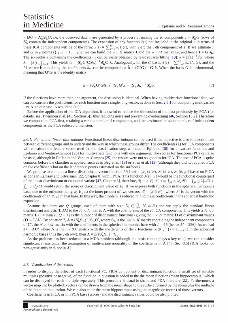
FPCA is carried out to describe the variability. The first three principal components explain 49.48% of the wholevariance, made up of 24.73%, 14.15% and 10.60% respectively. 91.27% of the variability is explained by the first sixteencomponents. Figure3 presents visual representations of the shape variation along the first three principal components.Figures in the supplementary material can help to interpretthem. The first component correspond to a size component,mostly concentrated on the head and the tail, but also in the body. 45.25% of the variation in this component is due to thex-coordinates (27.17% and 27.58% due to they andz-coordinates). Component 2 is focused on a part of the tail. In thiscomponent, 20.37% of variability comes from they-coordinates, and the rest is divided between thex andz-coordinates.Finally, the third component is concentrated almost entirely on the whole tail. The proportion of the variability in thiscomponent is 41.81% for they-coordinates (23.51% and 34.67% due to thex andz-coordinates).

It is interesting to distinguish between patients with AD, MCI and elderly CN subjects, however in the literature itis quite common to consider the pair-wise comparisons amongthe three groups. The important CN-MCI subproblemis analyzed here, together with the numerical results for the three group problem. For a detailed analysis of the otherproblems, see the supplementary material.

In order to test the ability to classify the subjects into their correct group, cross-validation is performed using leave-one-out trials. In each trial, one subject is set aside and FPCA is performed on the remaining subjects (the training set).On the one hand, the LDA classifier is trained with the firstJ PC scores of the training set. On the other hand, wecompute (and record) the leave-one-out (LOU) prediction error for that training set. The test subject is projected ontothesame principal components obtained from training set alone, and classified with the trained LDA. This predicted class ispreserved to produce the LOU estimate of the correct classification percentage forJ components, since this process isrepeated in turn for each of the subjects. Note that as FPCA iscomputed with different data, PCs from different iterationsare not comparable, especially those with low variance. We have the estimated accuracy for various values of the numberJ of principal components. In order to select the appropriatenumber of components, we do not choose the best result,as the accuracy would be too optimistic, but a double or nested cross-validation is done. We consider the recorded LOUprediction errors for each training set, and build a matrix with them. The number of rows is the number of subjects whereasthe number of columns is the total number of valuesJ considered. We compute the mean for each column, and the model(valueJ) selected is that one which gives the smallest mean (in case of tie, we select that with less components, the mostparsimonious). Hence, the estimated classification accuracy is the estimated accuracy by LOU for the model selected bythe nested LOU. Table2 shows the results for FPCA together with the rest of methods for the CN vs MCI problem. In thesupplementary material a table with the mean and standard deviation for each column of the matrix can be seen, and alsoa table with the external LOU accuracies for differentJ values.

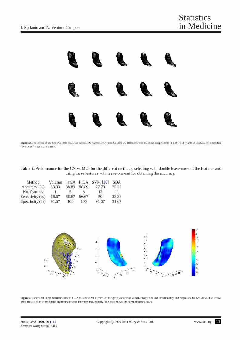
The same cross-validation strategy considered for FPCA is followed with FICA, whose results are displayed in Table2. Furthermore, we have computed the functional linear discriminant using all the subjects in the set for the number ofcomponents selected (J = 6 in this subproblem). In Figure4 it is visualized as explained in Sec.2.7. It suggests a small lossin the CA1 and a part of the subiculum in the body of the hippocampus. The discriminant function significantly separatesthe groups (Wilks’Λ = 0.197, p-value = 0.002).


http://www3.uji.es/~epifanio/RESEARCH/alzfda.rar

http://www.math.mcgill.ca/keith/surfstat

http://www.stat.wisc.edu/~mchung/research/amygdala/


3.2. Comparative performance

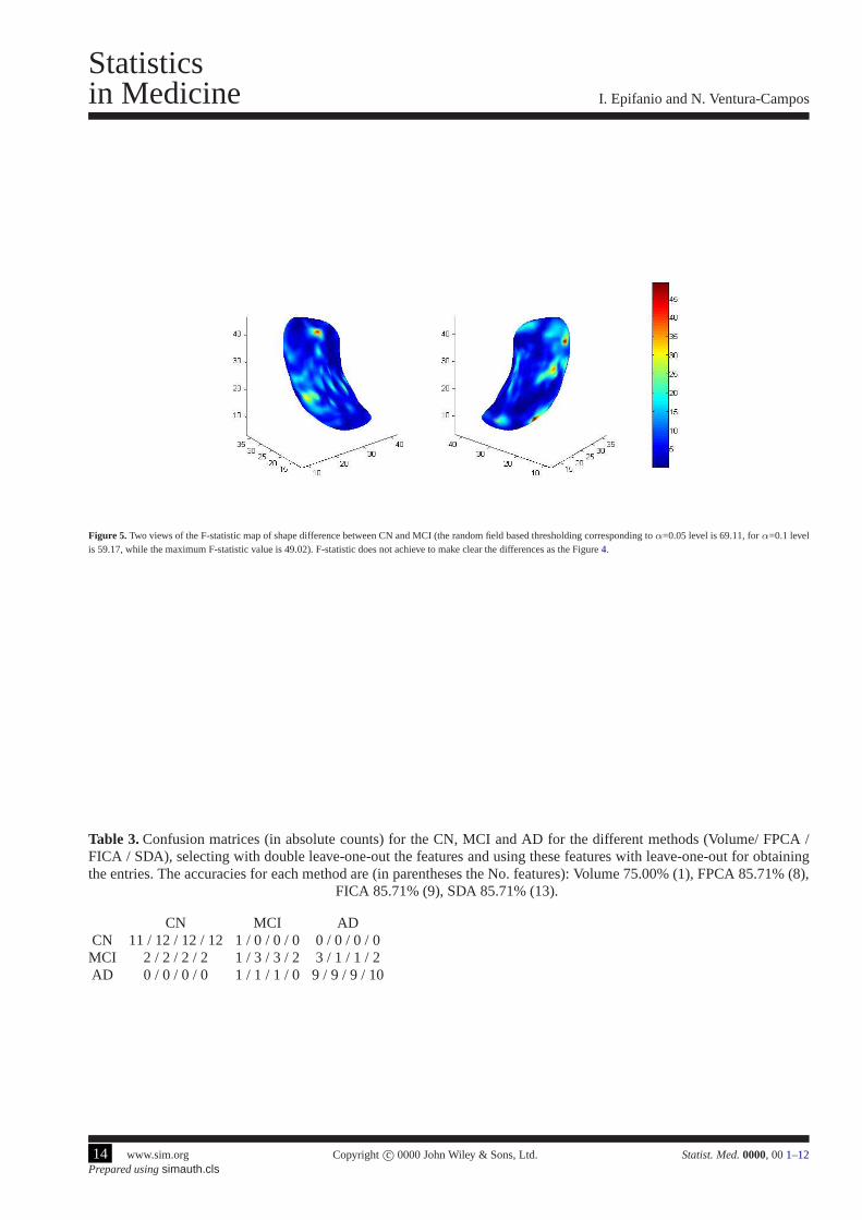
We reproduce the methodology in Chung et al. [17] with our data. We perform multivariate linear modeling [51] on ourspherical harmonic representation, testing the effect of group variable in the model. There is no statistically significantshape difference atα=0.05 when we test for group differences at each vertex of thehippocampal surface (see Figure5displaying the F-statistic value on the mean hippocampus).Although testing of group mean difference and discriminantanalysis are different problems (note that the coefficientsfor the discriminant function in MDA are derived so as tomaximize the differences between the group means), we have included this result for highlighting the utility of theproposed discriminant function since significance maps of group differences usually appear in neuroimaging literaturetogether with classification results [16].

The methodology in Gerardin et al. [16] is applied to our data: the SPHARM coefficients are classified with a supportvector machine (SVM). Student’st-tests were used for determining which coefficients best separate the groups, with abagging strategy (we use the same strategy but with the absolute value of thet statistic for really keeping only thosecoefficients which are always significantly different sinceit is a two tailed test). The result obtained with LOU is in Table2. The number of coefficients is selected by nested LOU. A linear kernel is considered, since better results are obtainedthan with radial basis functions with different scaling factors.

Recently, Clemmensen et al. [52] have proposed a sparse discriminant analysis (SDA) for thehigh-dimensional setting(the number of variables is large relative to the number of subjects). This method performs linear discriminant analysiswith a sparseness criterion imposed such that classification and feature selection are performed simultaneously. SDA isapplied to our SPHARM coefficients. We use the sparseLDA package with default parameters (except for the desirednumber of coefficients to be selected), which is available from http://www2.imm.dtu.dk/∼lhc/. The result obtained withLOU is in Table2. The number of coefficients is chosen by nested LOU.

Beg et al. [18] proposed four shape features for discriminating CN vs MCI with left hippocampi. They reported thefollowing accuracies for each set of features: 68.1% for 3D moment invariants features, 75% for 3D tensor invariantfeatures, 77.3% for 3D Laplacian invariant features, and 86.3% for 3D geodesic shape invariants features. Note that intheir database there are 26 CN and 18 MCI (a proportion similar to our database). Although results should be comparedwith caution since the databases are different, FPCA and FICA obtain better accuracies.

Other approaches, such as that in Shen et al. [13], evaluate the spherical representation in a serie of parameter locations,obtaining the coordinates on the surface, and work with these landmarks (SPHARM-PDM from Point Distribution Model)for classification. We do not consider this approach since itis well-known that some regularization is necessary in order toobtain meaningful results [19, Ch. 11], [22, Ch. 8]. In fact, in Figure5, where each spatial location is considered separately,there are a lot of small spots. However, in Figure4 the discriminative zones are larger and more homogeneous.

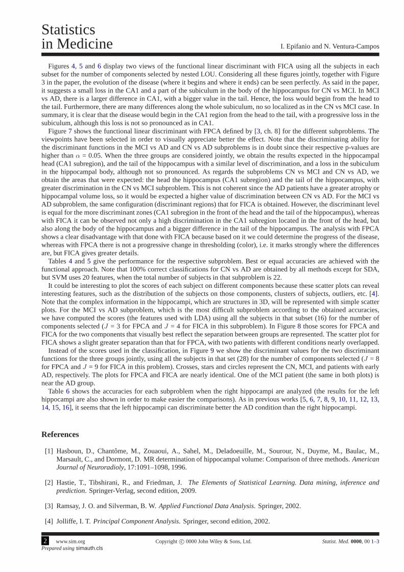
Table3 shows the confusion matrices for each method when the three groups are considered jointly, except for SVM inGerardin et al. [16], whose methodology is only for problems with two groups. Best or equal accuracies are achieved withthe functional approach. The CN group is correctly identified by FPCA, FICA and SDA, and SDA classifies correctly theAD group (there is only one misclassification is this group for the rest of methods, which classified an AD individual asMCI). The main errors are in the MCI group: with volumen only one individual is correctly identified in this group (twoindividuals are misclassified as CN and three as AD); with SDAtwo individuals are misclassified as CN and other two asAD, while the less number of errors are achieved with FPCA andFICA, where two individuals are misclassified as CNand one as AD. The two MCI individuals misclassified as CN are the same for all the methods, as well as the misclassifiedMCI individual as AD for FPCA and FICA.

4. Conclusions

Our novel contribution is to model the 3D hippocampal surfaces with a FDA approach, as hippocampi are in fact functionsdefined over two spherical angles. This approach allows to carry out the same analysis as any other branch of statistics[19]. As there are few studies with functional data with more than one argument, we have extended the functional datamethodology for functions with two arguments (angles in this case), introducing FICA for the first time. FPCA and FICAwith two arguments have been used for shape description and classification. A functional linear discriminant with FICAhas been also defined. To the best of our knowledge it has been used for the first time in localizing the differences amonggroups instead of the significance maps, and meaningful results are obtained with it. The functional linear discriminantwith FICA has given more details and coherence than that withFPCA (see the supplementary material). Classificationresults are better with FPCA and FICA (both with identical results), than the other alternatives considered, showing thatfeature extraction is a powerful method [53, Sec. 5.3.]. The same conclusions are reached with the othersubproblemconsidered in supplementary material. The good results in this important problem are other of our main contributions:in Table2 higher accuracy, sensitivity and specificity is achieved with the FDA approach (FPCA and FICA) than with


http://www2.imm.dtu.dk/~lhc/



other alternatives, even with a fewer number of features (except for volume which is univariate). We have focused onthe analysis of left hippocampi, as they seem to discriminate AD condition better than the right hippocampi (see thesupplementary material). As future work, it would be interesting to analyze the hippocampal asymmetry between left andright hippocampus in AD (as made for example with schizophrenia in [54]), using FDA and exploiting the potential ofthis perspective.

Our sample size is small and we use LOU (with nested LOU for selecting the number of features) for assessing themethod. With a larger database could be possible to split thedata into a training, validation and test set, and instead ofselecting the number of features, the features could be selected [48, Sec. 8.9.], and classification results could be improved.

The FDA approach is not restricted to hippocampi, it could beused with other structures. Furthermore, our methodologycould be extended to deal with functional data combined withmultivariate random variables. Ramsay and Silverman[19, Ch. 10] defined FPCA of hybrid data (univariate functions with one argument together with a vector). Maybe it isinteresting to consider the age, the education years or the intracranial volume, etc.

Finally, other interesting future topic includes using theFDA approach in other problems (such as Functional ANOVAor detection of outliers) with 3D shapes, for example for assessing the evolution along time in the same subjects in alongitudinal study.

Acknowledgments

The authors thank M. A. Garcıa and J. Epifanio and C.Avila for their support. This research was supported by grantsfrom the Spanish Ministerio de Ciencia e Innovacion (PSI2010-20294 CONSOLIDER-INGENIO 2010 Programme CDS-2007-00012), CICYT TIN2009-14392-C02-01, MTM2009-14500-C02-02, GV/2011/004 and Bancaixa-UJI P11A2009-02. The authors also thanks the Associate Editor and two reviewers for their very constructive suggestions, which led toimprovements in the manuscript.Conflict of Interest: None declared.

References

[1] Grundman, M., Petersen, R., Ferris, S., Thomas, R., Aisen, P., Bennet, D., Foster, N., Jack, C., Galasho, D., Dondy,R., Kaye, J., and Sano, M. Mild cognitive impairment can be distinguished from Alzheimer disease and normalaging for clinical trials.Archives of Neurology, 61:59–66, 2004.

[2] Petersen, R. C. Mild cognitive impairment as a diagnostic entity.Journal of Internal Medicine, 256:183–194, 2004.

[3] Jack, C. R., Petersen, R. C., Xu, Y. C., O’Brien, P. C., Smith, G. E., Ivnik, R. J., Boeve, B. F., Waring, S. C., Tangalos,E. G., and Kokmen, E. Prediction of AD with MRI-based hippocampal volume in mild cognitive impairment.Neurology, 52:1397–1403, 1999.

[4] Mungas, D., Jagust, W. J., Reed, B. R., Kramer, J. H., Weiner, M. W., Schuff, N., Norman, D., Mack, W. J., Willis,L., and Chui, H. C. MRI predictors of cognition in subcortical ischemic vascular disease and Alzheimer’s disease.Neurology, 57:2229–2235, 2001.

[5] Styner, M., Lieberman, J. A., Pantazis, D., and Gerig, G.Boundary and medial shape analysis of the hippocampusin schizophrenia.Medical Image Analysis Journal, 8(3):197–203, 2004.

[6] Styner, M., Gerig, G., Joshi, S. C., and Pizer, S. M. Automatic and robust computation of 3D medial modelsincorporating object variability.International Journal of Computer Vision, 55(2-3):107–122, 2003.

[7] Golland, P., Grimson, W. E. L., Shenton, M. E., and Kikinis, R. Deformation analysis for shape based classification.In Proceedings of the 17th International Conference on Information Processing in Medical Imaging, IPMI ’01, pages517–530, 2001. ISBN 3-540-42245-5.

[8] Joshi, S. C., Miller, M. I., and Grenander, U. On the geometry and shape of brain sub-manifolds.Internation Journalof Pattern Recognition and Artificial Intelligence, 11(8):1317–1343, 1997.

[9] Park, Y., Priebe, C. E., Miller, M. I., Mohan, N. R., and Botteron, K. N. Statistical analysis of twin populations usingdissimilarity measurements in hippocampus shape space.Journal of Biomedicine and Biotechnology, 2008(ArticleID 694297, doi:10.1155/2008/694297):5 pages, 2008.



[10] Shen, K., Fripp, J., Meriaudeau, F., Chetelat, G., Salvado, O., and Bourgeat, P. Detecting global and localhippocampal shape changes in Alzheimer’s disease using statistical shape models.NeuroImage, 59(3):2155–2166,2012.

[11] Gerig, G., Styner, M., Jones, D., Weinberger, D., and Lieberman, J. Shape analysis of brain ventricles usingSPHARM. In Proceedings of the IEEE Workshop on Mathematical Methods inBiomedical Image Analysis(MMBIA’01), pages 171–178, 2001.

[12] Gu, X., Wang, Y., Chan, T. F., Thompson, P. M., and Yau, S.Genus zero surface conformal mapping and itsapplication to brain surface mapping.IEEE Transactions on Medical Imaging, 23(8):949–958, 2004.

[13] Shen, L., Ford, J., Makedon, F., and Saykin, A. A surface-based approach for classification of 3D neuroanatomicstructures.Intelligent Data Analysis, 8(6):519–542, 2004.

[14] Chung, M. K., Dalton, K. M., Shen, L., Evans, A. C., and Davidson, R. J. Weighted fourier series representation andits application to quantifying the amount of gray matter.IEEE Transactions on Medical Imaging, 26(4):566–581,2007.

[15] L. Shen, H. F. and McPeek, M. Modeling 3-dimensional morphological structures using spherical harmonics.Evolution, 4(63):1003–1016, 2009.

[16] Gerardin, E., Chetelat, G., Chupin, M., Cuingnet, R., Desgranges, B., Kim, H., Niethammer, M., Dubois, B.,Lehericy, S., Garnero, L., Eustache, F., and Colliot, O. Multidimensional classification of hippocampal shapefeatures discriminates Alzheimer’s disease and mild cognitive impairment from normal aging.NeuroImage, 47(4):1476–1486, 2009.

[17] Chung, M. K., Worsley, K. J., Nacewicz, B. M., Dalton, K.M., and Davidson, R. J. General multivariate linearmodeling of surface shapes using surfstat.NeuroImage, 53(2):491–505, 2010.

[18] Beg, M. F., Raamana, P. R., Barbieri, S., and Wang, L. Comparison of four shape features for detecting hippocampalshape changes in early Alzheimers.Statistical Methods in Medical Research, published online 30 May 2012(DOI:10.1177/0962280212448975):1–24, 2012.

[19] Ramsay, J. O. and Silverman, B. W.Functional Data Analysis. Springer, 2nd edition, 2005.

[20] Ferraty, F. and Vieu, P.Nonparametric Functional Data Analysis: Theory and Practice. Springer, 2006.

[21] Ferraty, F. and Romain, Y.The Oxford Handbook of functional data analysis. Oxford University Press, 2011.

[22] Ramsay, J. O. and Silverman, B. W.Applied Functional Data Analysis. Springer, 2002.

[23] Luo, W., Cao, J., Gallagher, M., and Wiles, J. Estimating the intensity of ward admission and its effect on emergencydepartment access block.Statistics in Medicine, To appear(doi: 10.1002/sim.5684), 2012.

[24] Zhou, Y. and Sedransk, N. A new functional data-based biomarker for monitoring cardiovascular behavior.Statisticsin Medicine, 32(1):153164, 2013.

[25] Epifanio, I. and Ventura-Campos, N. Functional data analysis in shape analysis.Computational Statistics & DataAnalysis, 55(9):2758–2773, 2011.

[26] Stoyan, D. and Stoyan, H.Fractals, Random Shapes and Point Fields. Methods of Geometrical Statistics. Wiley,1994.

[27] Watson, C., Andermann, F., Gloor, P., Jones-Gotman, M., Peter, T., A., E., Olivier, A., Melanson, D., and G., L.Anatomic basis of amygdaloid and hippocampal volume measurement by magnetic resonance imaging.Neurology,42(9):1743–1750, 1992.

[28] Hasboun, D., Chantome, M., Zouaoui, A., Sahel, M., Deladoeuille, M., Sourour, N., Duyme, M., Baulac, M.,Marsault, C., and Dormont, D. MR determination of hippocampal volume: Comparison of three methods.AmericanJournal of Neuroradioly, 17:1091–1098, 1996.

[29] Kindratenko, V. V. On using functions to describe the shape. Journal of Mathematical Imaging and Vision, 18:225–245, 2003.




[30] Timsari, B. and Leahy, R. M. Optimization method for creating semi-isometric flat maps of the cerebral cortex. InProc. SPIE, Medical Imaging, volume 3979, pages 698–708, 2000.

[31] Brechbuhler, C., Gerig, G., and Kubler, O. Parametrization of closed surfaces for 3-D shape description.ComputerVision and Image Understanding, 61(2):154–170, 1995.

[32] Macdonald, D., Kabani, N., Avis, D., and Evans, A. C. Automated 3-D extraction of inner and outer surfaces ofcerebral cortex from MRI.NeuroImage, 12(3):340–356, 2000.

[33] Alfeld, P., Neamtu, M., and Schumaker, L. L. Fitting scattered data on sphere-like surfaces using spherical splines.Journal of Computational and Applied Mathematics, 73(1-2):5–43, 1996.

[34] He, Y., Li, X., Gu, X., and Qin, H. Brain image analysis using spherical splines. InProc. of Energy MinimizationMethods in Computer Vision and Pattern Recognition, pages 633–644, 2005.

[35] Nain, D., Styner, M., Niethammer, M., Levitt, J. J., Shenton, M., Gerig, G., and Tannenbaum, A. Statistical shapeanalysis of brain structures using spherical wavelets. InProceedings of the Fourth IEEE International Symposiumon Biomedical Imaging, page 209–212, 2007.

[36] Yu, P., Grant, P. E., Qi, Y., Han, X., Segonne, F., Pienaar, R., Busa, E., Pacheco, J., Makris, N., Buckner, R. L.,Golland, P., and Fischl, B. Cortical surface shape analysisbased on spherical wavelets.IEEE Transactions onMedical Imaging, 26(4):582 – 597, 2007.

[37] Kneip, A. and Ramsay, J. O. Combining registration and fitting for functional models.Journal of the AmericanStatistical Association, 103(483):1155–1165, 2008.

[38] Epifanio, I. Shape descriptors for classification of functional data.Technometrics, 50(3):284–294, 2008.

[39] Hastie, T., Buja, A., and Tibshirani, R. Penalized discriminant analysis.Annals of Statistics, 23:73–102, 1995.

[40] Ferraty, F. and Vieu, P. Curves discrimination: a nonparametric functional approach.Computational Statistics andData Analysis, 44:161–173, 2003.

[41] Rossi, F. and Conan-Guez, B. Functional multi-layer perceptron: a nonlinear tool for functional data analysis.NeuralNetworks, 18(1):45–60, 2005.

[42] Ferre, L. and Villa, N. Multilayer perceptron with functional inputs: an inverse regression approach.ScandinavianJournal of Statistics, 33(4):807–823, 2006.

[43] Rossi, F. and Villa, N. Support vector machine for functional data classification.Neurocomputing, 69(7–9):730–742,2006.

[44] Li, B. and Yu, Q. Classification of functional data: A segmentation approach.Computational Statistics and DataAnalysis, 52:4790–4800, 2008.

[45] Hyvarinen, A., Karhunen, J., and Oja, E. Independent component analysis: Algorithms and applications.NeuralNetworks, 13:411–430, 2000.

[46] Hyvarinen, A., Karhunen, J., and Oja, E.Independent component analysis. Wiley, New York, 2001.

[47] Ripley, B. D. Pattern recognition and neural networks. Cambridge University Press, 1996.

[48] Rencher, A. C.Methods of Multivariate Analysis. Wiley, 2nd edition, 2002.

[49] Hyvarinen, A. Fast and robust fixed-point algorithms for indepent component analysis, http://www.cis.hut.fi/projects/ica/fastica/.IEEE Transactions on Neural Networks, 10(3):626–634, 1999.

[50] Muller, M. J., Greverus, D., Weibrich, C., Dellani, P.R., Scheurich, A., Stoeter, P., and Fellgiebel, A. Diagnosticutility of hippocampal size and mean diffusivity in amnestic MCI. Neurobiology of Aging, 28(3):398–403, 2007.

[51] Taylor, J. and Worsley, K. Random fields of multivariatetest statistics, with applications to shape analysis.Annalsof Statistics, 36(1):1–27, 2008.

[52] Clemmensen, L., Hastie, T., Witten, D., and B., E. Sparse discriminant analysis.Technometrics, 53(4):406–413,2011.



[53] Hastie, T., Tibshirani, R., and Friedman, J.The Elements of Statistical Learning. Data mining, inference andprediction. Springer-Verlag, second edition, 2009.

[54] Wang, L., Joshi, S., Miller, M., and Csernansky, J. Statistical analysis of hippocampal asymmetry in schizophrenia.Neuroimage, 14(3):531–45, 2001.

5. Figures and Tables

Table 1.Description of the database. The number inside the parentheses is the standard deviation.

CN,N1 = 12 MCI,N2 = 6 AD, N3 = 10Sex (Male/Female) 5/7 2/4 1/9

Mean age 70.17 (3.43) 75.50 (3.33) 71.5 (4.35)Mean CDR (Clinical Dementia Rating) 0 (0) 0.5 (0) 0.95 (0.15)

(a) (b)

Figure 1. Hippocampal outlines in a coronal (a) and sagittal (b) slice.

Figure 2. For one hippocampus: (A) the surface flattening process fromthe original one in the top left of the figure to the bottom right. The same level sets as in [17] are used(1.0, 0.6, 0.2, -0.2, -0.6, -1.0). (B) The spherical angles projected onto the hippocampus surface (forθ andϕ respectively), together with a unit sphere showing the angles. (C) Thespherical harmonic representations of the hippocampus surface forL = 1, 2, 8, 15, 30 (from left to right).




Figure 3. The effect of the first PC (first row), the second PC (second row) and the third PC (third row) on the mean shape: from -2 (left)to 2 (right) in intervals of 1 standarddeviations for each component.

Table 2.Performance for the CN vs MCI for the different methods, selecting with double leave-one-out the features andusing these features with leave-one-out for obtaining the accuracy.

Method Volume FPCA FICA SVM [16] SDAAccuracy (%) 83.33 88.89 88.89 77.78 72.22No. features 1 5 6 12 11

Sensitivity (%) 66.67 66.67 66.67 50 33.33Specificity (%) 91.67 100 100 91.67 91.67

Figure 4. Functional linear discriminant with FICA for CN vs MCI (fromleft to right): vector map with the magnitude and directionality, and magnitude for two views. The arrowsshow the direction in which the discriminant score increases most rapidly. The color shows the norm of those arrows.



Figure 5. Two views of the F-statistic map of shape difference betweenCN and MCI (the random field based thresholding corresponding toα=0.05 level is 69.11, forα=0.1 levelis 59.17, while the maximum F-statistic value is 49.02). F-statistic does not achieve to make clear the differences as the Figure4.

Table 3.Confusion matrices (in absolute counts) for the CN, MCI and AD for the different methods (Volume/ FPCA /FICA / SDA), selecting with double leave-one-out the features and using these features with leave-one-out for obtainingthe entries. The accuracies for each method are (in parentheses the No. features): Volume 75.00% (1), FPCA 85.71% (8),

FICA 85.71% (9), SDA 85.71% (13).

CN MCI ADCN 11 / 12 / 12 / 12 1 / 0 / 0 / 0 0 / 0 / 0 / 0MCI 2 / 2 / 2 / 2 1 / 3 / 3 / 2 3 / 1 / 1 / 2AD 0 / 0 / 0 / 0 1 / 1 / 1 / 0 9 / 9 / 9 / 10


Research Article


Received XXXX

(www.interscience.wiley.com) DOI: 10.1002/sim.0000

Supplementary material to “Hippocampal shapeanalysis in Alzheimer’s disease using FunctionalData Analysis”

Irene Epifanioa∗, Noelia Ventura-Camposb

1. Introduction

This Supplementary Material contains the analysis of the ADpatients versus CN and versus MCI and the analysis for thethree groups: CN, MCI and patients with early AD.

2. Results

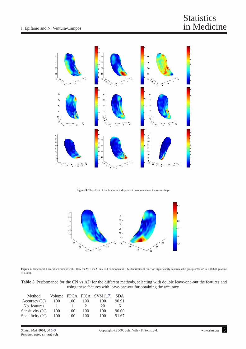
Figure1 shows the magnitude of the first three principal component over the mean hippocampus for the whole database.The viewpoints have been selected in order to visually appreciate better the effect. As code and data are available athttp://www3.uji.es/∼epifanio/RESEARCH/alzfda.rar, figures can be reproduced and the view can be interactively rotated.Head, body and tail are the three parts that make up a hippocampus [1]. A schematic representation of the hippocampalsubfields is shown in Figure2, which can help in the interpretation. Analogously, Figure3 shows the magnitude of thefirst nine independent components over the mean hippocampusfor the whole database. The effect for the first and thirdcomponents is distributed along the whole hippocampus except the more extreme zones of the tail and head; while the restof components are concentrated in different parts of the hippocampus: tail (second, seventh, eighth and ninth), subiculum(fifth and sixth), and head (fourth).

Table1 gives the accuracies for the CN vs MCI problem using different values ofL for representing the hippocampi.Note that the results are similar to those obtained withL =15, but whenL increases (forL bigger than the chosenL =15) the performances are a bit worse, maybe because we could be fitting noise. For smallL the performances are similar.Curiously withL = 3 the numerical results are a bit better, but it would not be possible to appreciate where the differencesare with the functional linear discriminant, since withL = 3 the degree of smoothing is very high (see Figure 2 in thepaper).

Table 2 gives the summary analysis of the accuracies for the nested LOU (the recorded LOU prediction errors foreach training set) for different values ofJ in the CN vs MCI subproblem. The biggest mean accuracy for each methodcorresponds with one of the smallest standard deviation. Note that these accuracies are bigger than those reported inTable 2 of the paper, since these accuracies are computed with each training set, and therefore they are overestimatedsometimes substantially [2, ch. 7], while in Table 2 of the paper the external LOU resultsare reported (each test subject isa completely new data not used in the analysis or the selection of the model, for ascertaining the generalization capabilityof the classifier). In Table3 the accuracies for the external LOU for different values ofJ are shown (the selected ones bythe nested LOU, whose performances appear in Table 2 of the paper, are in a frame box).

a Dept. Matematiques, Universitat Jaume I, Campus del Riu Sec, 12071 Castello, Spainb Dept. Psicologia Basica, Clınica i Psicobiologia, Universitat Jaume I, Spain∗Correspondence to: Tel.: +34-964728390, fax: +34-964728429. E-mail: [email protected]

Statist. Med.0000, 001–3 Copyright c© 0000 John Wiley & Sons, Ltd.

Prepared usingsimauth.cls [Version: 2010/03/10 v3.00]

http://www3.uji.es/~epifanio/RESEARCH/alzfda.rar


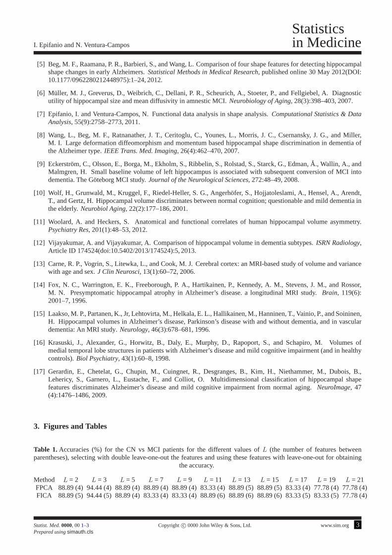
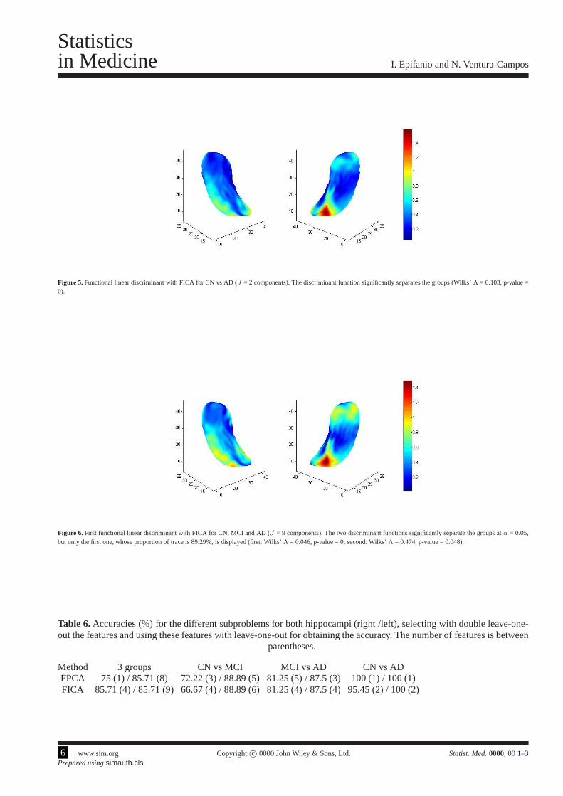
Figures4, 5 and6 display two views of the functional linear discriminant with FICA using all the subjects in eachsubset for the number of components selected by nested LOU. Considering all these figures jointly, together with Figure3 in the paper, the evolution of the disease (where it begins and where it ends) can be seen perfectly. As said in the paper,it suggests a small loss in the CA1 and a part of the subiculum in the body of the hippocampus for CN vs MCI. In MCIvs AD, there is a larger difference in CA1, with a bigger valuein the tail. Hence, the loss would begin from the head tothe tail. Furthermore, there are many differences along thewhole subiculum, no so localized as in the CN vs MCI case. Insummary, it is clear that the disease would begin in the CA1 region from the head to the tail, with a progressive loss in thesubiculum, although this loss is not so pronounced as in CA1.

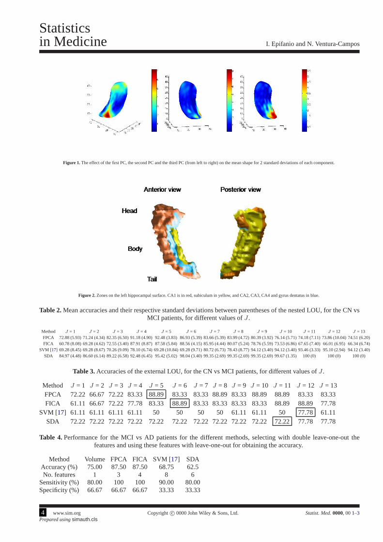
Figure7 shows the functional linear discriminant with FPCA defined by [3, ch. 8] for the different subproblems. Theviewpoints have been selected in order to visually appreciate better the effect. Note that the discriminating ability forthe discriminant functions in the MCI vs AD and CN vs AD subproblems is in doubt since their respective p-values arehigher thanα = 0.05. When the three groups are considered jointly, we obtain the results expected in the hippocampalhead (CA1 subregion), and the tail of the hippocampus with a similar level of discrimination, and a loss in the subiculumin the hippocampal body, although not so pronounced. As regards the subproblems CN vs MCI and CN vs AD, weobtain the areas that were expected: the head the hippocampus (CA1 subregion) and the tail of the hippocampus, withgreater discrimination in the CN vs MCI subproblem. This is not coherent since the AD patients have a greater atrophy orhippocampal volume loss, so it would be expected a higher value of discrimination between CN vs AD. For the MCI vsAD subproblem, the same configuration (discriminant regions) that for FICA is obtained. However, the discriminant levelis equal for the more discriminant zones (CA1 subregion in the front of the head and the tail of the hippocampus), whereaswith FICA it can be observed not only a high discrimination inthe CA1 subregion located in the front of the head, butalso along the body of the hippocampus and a bigger difference in the tail of the hippocampus. The analysis with FPCAshows a clear disadvantage with that done with FICA because based on it we could determine the progress of the disease,whereas with FPCA there is not a progressive change in thresholding (color), i.e. it marks strongly where the differencesare, but FICA gives greater details.

Tables4 and5 give the performance for the respective subproblem. Best orequal accuracies are achieved with thefunctional approach. Note that 100% correct classifications for CN vs AD are obtained by all methods except for SDA,but SVM uses 20 features, when the total number of subjects inthat subproblem is 22.

It could be interesting to plot the scores of each subject on different components because these scatter plots can revealinteresting features, such as the distribution of the subjects on those components, clusters of subjects, outliers, etc. [4].Note that the complex information in the hippocampi, which are structures in 3D, will be represented with simple scatterplots. For the MCI vs AD subproblem, which is the most difficult subproblem according to the obtained accuracies,we have computed the scores (the features used with LDA) using all the subjects in that subset (16) for the number ofcomponents selected (J = 3 for FPCA andJ = 4 for FICA in this subproblem). In Figure8 those scores for FPCA andFICA for the two components that visually best reflect the separation between groups are represented. The scatter plot forFICA shows a slight greater separation than that for FPCA, with two patients with different conditions nearly overlapped.

Instead of the scores used in the classification, in Figure9 we show the discriminant values for the two discriminantfunctions for the three groups jointly, using all the subjects in that set (28) for the number of components selected (J = 8for FPCA andJ = 9 for FICA in this problem). Crosses, stars and circles represent the CN, MCI, and patients with earlyAD, respectively. The plots for FPCA and FICA are nearly identical. One of the MCI patient (the same in both plots) isnear the AD group.

Table6 shows the accuracies for each subproblem when the right hippocampi are analyzed (the results for the lefthippocampi are also shown in order to make easier the comparisons). As in previous works [5, 6, 7, 8, 9, 10, 11, 12, 13,14, 15, 16], it seems that the left hippocampi can discriminate betterthe AD condition than the right hippocampi.

References

[1] Hasboun, D., Chantome, M., Zouaoui, A., Sahel, M., Deladoeuille, M., Sourour, N., Duyme, M., Baulac, M.,Marsault, C., and Dormont, D. MR determination of hippocampal volume: Comparison of three methods.AmericanJournal of Neuroradioly, 17:1091–1098, 1996.

[2] Hastie, T., Tibshirani, R., and Friedman, J.The Elements of Statistical Learning. Data mining, inference andprediction. Springer-Verlag, second edition, 2009.

[3] Ramsay, J. O. and Silverman, B. W.Applied Functional Data Analysis. Springer, 2002.

[4] Jolliffe, I. T. Principal Component Analysis. Springer, second edition, 2002.




[5] Beg, M. F., Raamana, P. R., Barbieri, S., and Wang, L. Comparison of four shape features for detecting hippocampalshape changes in early Alzheimers.Statistical Methods in Medical Research, published online 30 May 2012(DOI:10.1177/0962280212448975):1–24, 2012.

[6] Muller, M. J., Greverus, D., Weibrich, C., Dellani, P. R., Scheurich, A., Stoeter, P., and Fellgiebel, A. Diagnosticutility of hippocampal size and mean diffusivity in amnestic MCI. Neurobiology of Aging, 28(3):398–403, 2007.

[7] Epifanio, I. and Ventura-Campos, N. Functional data analysis in shape analysis.Computational Statistics & DataAnalysis, 55(9):2758–2773, 2011.

[8] Wang, L., Beg, M. F., Ratnanather, J. T., Ceritoglu, C., Younes, L., Morris, J. C., Csernansky, J. G., and Miller,M. I. Large deformation diffeomorphism and momentum based hippocampal shape discrimination in dementia ofthe Alzheimer type.IEEE Trans. Med. Imaging, 26(4):462–470, 2007.

[9] Eckerstrom, C., Olsson, E., Borga, M., Ekholm, S., Ribbelin, S., Rolstad, S., Starck, G., Edman,A., Wallin, A., andMalmgren, H. Small baseline volume of left hippocampus is associated with subsequent conversion of MCI intodementia. The Goteborg MCI study.Journal of the Neurological Sciences, 272:48–49, 2008.

[10] Wolf, H., Grunwald, M., Kruggel, F., Riedel-Heller, S.G., Angerhofer, S., Hojjatoleslami, A., Hensel, A., Arendt,T., and Gertz, H. Hippocampal volume discriminates betweennormal cognition; questionable and mild dementia inthe elderly.Neurobiol Aging, 22(2):177–186, 2001.

[11] Woolard, A. and Heckers, S. Anatomical and functional correlates of human hippocampal volume asymmetry.Psychiatry Res, 201(1):48–53, 2012.

[12] Vijayakumar, A. and Vijayakumar, A. Comparison of hippocampal volume in dementia subtypes.ISRN Radiology,Article ID 174524(doi:10.5402/2013/174524):5, 2013.

[13] Carne, R. P., Vogrin, S., Litewka, L., and Cook, M. J. Cerebral cortex: an MRI-based study of volume and variancewith age and sex.J Clin Neurosci, 13(1):60–72, 2006.

[14] Fox, N. C., Warrington, E. K., Freeborough, P. A., Hartikainen, P., Kennedy, A. M., Stevens, J. M., and Rossor,M. N. Presymptomatic hippocampal atrophy in Alzheimer’s disease. a longitudinal MRI study.Brain, 119(6):2001–7, 1996.

[15] Laakso, M. P., Partanen, K., Jr, Lehtovirta, M., Helkala, E. L., Hallikainen, M., Hanninen, T., Vainio, P., and Soininen,H. Hippocampal volumes in Alzheimer’s disease, Parkinson’s disease with and without dementia, and in vasculardementia: An MRI study.Neurology, 46(3):678–681, 1996.

[16] Krasuski, J., Alexander, G., Horwitz, B., Daly, E., Murphy, D., Rapoport, S., and Schapiro, M. Volumes ofmedial temporal lobe structures in patients with Alzheimer’s disease and mild cognitive impairment (and in healthycontrols).Biol Psychiatry, 43(1):60–8, 1998.

[17] Gerardin, E., Chetelat, G., Chupin, M., Cuingnet, R., Desgranges, B., Kim, H., Niethammer, M., Dubois, B.,Lehericy, S., Garnero, L., Eustache, F., and Colliot, O. Multidimensional classification of hippocampal shapefeatures discriminates Alzheimer’s disease and mild cognitive impairment from normal aging.NeuroImage, 47(4):1476–1486, 2009.

3. Figures and Tables

Table 1.Accuracies (%) for the CN vs MCI patients for the different values of L (the number of features betweenparentheses), selecting with double leave-one-out the features and using these features with leave-one-out for obtaining

the accuracy.

Method L = 2 L = 3 L = 5 L = 7 L = 9 L = 11 L = 13 L = 15 L = 17 L = 19 L = 21FPCA 88.89 (4) 94.44 (4) 88.89 (4) 88.89 (4) 88.89 (4) 83.33 (4) 88.89 (5) 88.89 (5) 83.33 (4) 77.78 (4) 77.78 (4)FICA 88.89 (5) 94.44 (5) 88.89 (4) 83.33 (4) 83.33 (4) 88.89 (6) 88.89 (6) 88.89 (6) 83.33 (5) 83.33 (5) 77.78 (4)



Figure 1. The effect of the first PC, the second PC and the third PC (from left to right) on the mean shape for 2 standard deviations of each component.

Figure 2. Zones on the left hippocampal surface. CA1 is in red, subiculum in yellow, and CA2, CA3, CA4 and gyrus dentatus in blue.

Table 2.Mean accuracies and their respective standard deviations between parentheses of the nested LOU, for the CN vsMCI patients, for different values ofJ .

Method J = 1 J = 2 J = 3 J = 4 J = 5 J = 6 J = 7 J = 8 J = 9 J = 10 J = 11 J = 12 J = 13FPCA 72.88 (5.93) 71.24 (4.34) 82.35 (6.50) 91.18 (4.90) 92.48 (3.83) 86.93 (5.39) 83.66 (5.39) 83.99 (4.72) 80.39 (3.92) 76.14 (5.71) 74.18 (7.11) 73.86 (10.04) 74.51 (6.20)FICA 60.78 (8.08) 69.28 (4.62) 72.55 (3.40) 87.91 (8.87) 87.58 (5.84) 88.56 (4.15) 85.95 (4.44) 80.07 (5.24) 78.76 (5.59) 73.53 (6.86) 67.65 (7.40) 66.01 (6.95) 66.34 (6.74)

SVM [17] 69.28 (8.45) 69.28 (8.67) 70.26 (9.09) 78.10 (6.74) 69.28 (10.84) 69.28 (9.71) 80.72 (6.73) 78.43 (8.77) 94.12 (3.40) 94.12 (3.40) 93.46 (3.33) 95.10 (2.94) 94.12 (3.40)SDA 84.97 (4.48) 86.60 (6.14) 89.22 (6.58) 92.48 (6.45) 95.42 (5.02) 98.04 (3.40) 99.35 (2.69) 99.35 (2.69) 99.35 (2.69)99.67 (1.35) 100 (0) 100 (0) 100 (0)

Table 3.Accuracies of the external LOU, for the CN vs MCI patients, for different values ofJ .

Method J = 1 J = 2 J = 3 J = 4 J = 5 J = 6 J = 7 J = 8 J = 9 J = 10 J = 11 J = 12 J = 13FPCA 72.22 66.67 72.22 83.3388.89 83.33 83.33 88.89 83.33 88.89 88.89 83.33 83.33FICA 61.11 66.67 72.22 77.78 83.3388.89 83.33 83.33 83.33 83.33 88.89 88.89 77.78

SVM [17] 61.11 61.11 61.11 61.11 50 50 50 50 61.11 61.11 5077.78 61.11SDA 72.22 72.22 72.22 72.22 72.22 72.22 72.22 72.22 72.22 72.22 72.22 77.78 77.78

Table 4.Performance for the MCI vs AD patients for the different methods, selecting with double leave-one-out thefeatures and using these features with leave-one-out for obtaining the accuracy.

Method Volume FPCA FICA SVM [17] SDAAccuracy (%) 75.00 87.50 87.50 68.75 62.5No. features 1 3 4 8 6

Sensitivity (%) 80.00 100 100 90.00 80.00Specificity (%) 66.67 66.67 66.67 33.33 33.33




Figure 3. The effect of the first nine independent components on the mean shape.

Figure 4. Functional linear discriminant with FICA for MCI vs AD (J = 4 components). The discriminant function significantly separates the groups (Wilks’Λ = 0.320, p-value= 0.008).

Table 5.Performance for the CN vs AD for the different methods, selecting with double leave-one-out the features andusing these features with leave-one-out for obtaining the accuracy.

Method Volume FPCA FICA SVM [17] SDAAccuracy (%) 100 100 100 100 90.91No. features 1 1 2 20 6

Sensitivity (%) 100 100 100 100 90.00Specificity (%) 100 100 100 100 91.67



Figure 5. Functional linear discriminant with FICA for CN vs AD (J = 2 components). The discriminant function significantly separates the groups (Wilks’Λ = 0.103, p-value =0).

Figure 6. First functional linear discriminant with FICA for CN, MCI and AD (J = 9 components). The two discriminant functions significantly separate the groups atα = 0.05,but only the first one, whose proportion of trace is 89.29%, isdisplayed (first: Wilks’Λ = 0.046, p-value = 0; second: Wilks’Λ = 0.474, p-value = 0.048).

Table 6.Accuracies (%) for the different subproblems for both hippocampi (right /left), selecting with double leave-one-out the features and using these features with leave-one-out for obtaining the accuracy. The number of features is between

parentheses.

Method 3 groups CN vs MCI MCI vs AD CN vs ADFPCA 75 (1) / 85.71 (8) 72.22 (3) / 88.89 (5) 81.25 (5) / 87.5 (3)100 (1) / 100 (1)FICA 85.71 (4) / 85.71 (9) 66.67 (4) / 88.89 (6) 81.25 (4) / 87.5(4) 95.45 (2) / 100 (2)




Figure 7. Top left: First functional linear discriminant with FPCA for CN, MCI and AD (J = 8 components), whose proportion of trace is 92.9% and Wilks’ Λ = 0.065, p-value= 0 (note that for the second functional linear discriminantthe p-value is higher thanα = 0.05, Wilks’Λ = 0.609, p-value = 0.154); Top right: Functional linear discriminant withFPCA for CN vs MCI (J = 5 components, Wilks’Λ = 0.266, p-value = 0.003); Bottom left: Functional linear discriminant with FPCA for MCI vs AD (J = 3 components, Wilks’Λ = 0.612, p-value = 0.105, note that the p-value is higher thanα = 0.05); Bottom right: Functional linear discriminant withFPCA for CN vs AD (J = 1 component, Wilks’Λ =0.959, p-value = 0.367, note that the p-value is higher thanα = 0.05).

−5 0 5 10−8

−6

−4

−2

0

2

4

6

8

−1.15 −1.1 −1.05 −1 −0.95 −0.9 −0.85 −0.8 −0.750.1

0.15

0.2

0.25

0.3

0.35

0.4

0.45

0.5

0.55

0.6

Figure 8. Scatter plot of scores for MCI vs AD. Component 1 vs 3 for FPCA (left) and component 2 vs 4 for FICA (right). Stars and circlesrepresent the MCI and patients withearly AD, respectively.



−5 0 5−4

−3

−2

−1

0

1

2

3

26 28 30 32 34 36 385

6

7

8

9

10

11

Figure 9. Scatter plot of discriminant values for the two discriminant functions of the three groups: FPCA (left) and FICA (right). Crosses, stars and circles represent the CN, MCI,and patients with early AD, respectively.


Documents

Título artículo / Títol article: Hippocampal shape ... · independent component analysis are deﬁned for multivariat e functions with two arguments. A functional linear ... Neuropsychology