Title Boundary cooperative control by flexible Timoshenko arms

Author(s) Endo, Takahiro; Matsuno, Fumitoshi; Jia, Yingmin

Citation Automatica (2017), 81: 377-389

Issue Date 2017-07

URL http://hdl.handle.net/2433/232625

Right

© 2017. This manuscript version is made available under theCC-BY-NC-ND 4.0 licensehttp://creativecommons.org/licenses/by-nc-nd/4.0/; The full-text file will be made open to the public on 01 July 2019 inaccordance with publisher's 'Terms and Conditions for Self-Archiving'; この論文は出版社版でありません。引用の際には出版社版をご確認ご利用ください。; This is not thepublished version. Please cite only the published version.

Type Journal Article

Textversion author

Kyoto University

1

Boundary Cooperative Control by Flexible Timoshenko Arms

Takahiro Endo*a, Fumitoshi Matsunoa, and Yingmin Jiab

* Corresponding author. Phone/Fax +81-75-383-3595 a Department of Mechanical Engineering and Science, Kyoto University, {endo, matsuno}@me.kyoto-u.ac.jp

b Seventh Research Division, Beihang University, ymjia@buaa.edu.cn

Abstract

This paper discusses a cooperative control problem by two one-link flexible Timoshenko arms. The goal is to control a grasping force to collect an object with the two flexible arms, and to simultaneously suppress the vibrations of the arms. To solve this problem, we propose a boundary controller that is based on a dynamic model represented by a hybrid PDE-ODE model; the exponential stability of the closed-loop system is then proven by the frequency domain method. Finally, several numerical simulations are carried out to investigate the validity of the proposed boundary cooperative controller.

Key words: Flexible arms, Cooperative control, Force control, Exponentially stable, Distributed parameter systems.

1. Introduction

A flexible arm is a controlled system modeled by partial differential equations (PDEs) to present the dynamics of the elastic links, and ordinary differential equations (ODEs) to present the dynamics of sensors, actuators, and tip loads. The dynamic model of the flexible arm is thus a hybrid PDE-ODE model. The Euler-Bernoulli beam model in particular is widely used to present the dynamics of the elastic links. On the other hand, the Timoshenko beam model is a modified model of the Euler-Bernoulli beam model that includes the effects of shear and rotational iner-tia. Therefore, the Timoshenko beam model can be used in a wider range of applications than the Euler-Bernoulli beam model (Huang, 1961; Han, Benaroya, & Wei, 1999). Here, the flexible arm, modeled as a Timoshenko beam, is called the flexible Timoshenko arm.

There have been several relevant studies about the flex-ible Timoshenko arm based on the hybrid PDE-ODE mod-el (Morgül, 1992; Zhang et al., 1997; Taylor & Yau, 2003; Macchelli & Melchiorri, 2004; Grobbelaar-Van Dalsen, 2010; He, Zhang, & Ge, 2013; Muñoz Rivera, & Ávila, 2015; Endo, Sasaki, & Matsuno, 2017; and references therein). However, many of these studies on hybrid PDE-ODE infinite dimensional settings address only the vibra-tion suppression problem. This is insufficient for use of the flexible arm for more complex tasks. In addition to the vi-bration control, the force control, that is the control of the contact force at the contact point where the flexible arm touches an object or the environment, is necessary for real-ization of more complex tasks (Yoshikawa, 2000; Hokayen & Spong, 2006). Very few studies, Endo, Sasaki, and Matsuno (2017) have investigated the force control prob-lem of the flexible Timoshenko arm.

This paper discusses the cooperative control problem of two one-link flexible Timoshenko arms modeled by hybrid PDE-ODE infinite dimensional model. This problem is a typical applied force control problem. In the cooperative control problem, two one-link flexible Timoshenko arms grasp an object, and the flexible arms control the contact-force at the contact point to achieve the desired grasping force. From the point of view of cooperative control, con-trol of grasping force must consider the following: how to control the internal force applied to the grasped object by the two flexible Timoshenko arms, and how to control the motion of the grasped object. For cooperative control of the flexible arms, it is necessary to suppress vibration in the arms, as well as to control the grasping force. Although there has been little research on the cooperative control of flexible arms, several studies have investigated the infinite dimensional settings (Matsuno & Hayashi, 2000; Morita et al., 2003; Endo, Matsuno, & Kawasaki, 2009; Dou & Wang, 2014). These studies (Matsuno & Hayashi, 2000; Morita et al., 2003; Endo, Matsuno, & Kawasaki, 2009), discussed the cooperative control by two one-link flexible arms modeled by the Euler-Bernoulli beam model, and proposed asymptotic/exponential stabilizing controllers. Dou and Wang (2014) had a slightly different focus, pro-posing a cooperative controller for a system in which two rigid arms grasp a flexible object modeled by the Euler-Bernoulli beam. To the best of our knowledge, however, there has been no study of cooperative control by the flexi-ble Timoshenko arms based on the hybrid PDE-ODE infi-nite dimensional model. As mentioned above, the Timo-shenko beam model is a modified model of the Euler-Bernoulli beam model, and its application range is wide. Thus, the cooperative control problem by two one-link flexible Timoshenko arms is a challenging and useful issue.

2

In this paper, we propose a simple boundary cooperative controller for the cooperative control of two one-link flexi-ble Timoshenko arms. Many boundary controllers have been proposed for various hybrid PDE-ODE infinite di-mensional models other than the flexible Timoshenko arm (e.g., Littman & Markus, 1988; Slemrod, 1989; d'Andréa-Novel et al., 1994; Luo, Guo, & Morgul, 1999; Matsuno, Ohno, & Orlov, 2002; Choi, Hong, & Yang, 2004; Yang, Hong, & Matsuno, 2005; Krstic & Smyshlyaev, 2008; Nguyen & Hong, 2010; He et al., 2011; Endo, Matsuno, & Kawasaki, 2014; Curtain & Zwart, 2016). In the boundary controller, the control action is at the boundary of the sys-tems. Consideration of the distributed controller of the hy-brid PDE-ODE model (e.g. Hong, 1997; He et al., 2016) reveals that implementation of the boundary controller is generally easy from a practical point of view. We therefore propose a boundary controller to solve the cooperative control problem by two one-link flexible Timoshenko arms modeled by the hybrid PDE-ODE model. The proposed system consists of two flexible Timoshenko arms installed on a slider. The two arms push an object toward each other from opposite sides using the same force; together they produce a positive internal force and the object is grasped by the flexible arms. In addition, the motion of the grasped object is realized by the motion of the slider. We prove that cooperative control is accomplished; that is, we prove the exponential stability of the closed-loop system by the fre-quency domain method. In addition, we consider the ro-bustness of the proposed boundary controller with respect to the disturbance at the grasped object and the control in-put. The paper is organized as follows: in the next section, we formulate the control problem and propose a simple boundary cooperative controller. Section 3 presents the semigroup setting of the closed-loop system. Exponential stability and the robustness are given in Section 4. The numerical simulation results, which demonstrate the validi-ty of the proposed boundary controller, are presented in Section 5. Finally, Section 6 contains our conclusions.

2. System description and boundary controller

2.1. A controlled system

Fig. 1 illustrates a controlled system. The system con-sists of two one-link flexible arms and a grasped object. One end of flexible arm i, 2 ,1=i , is clamped to the rota-tional motor i, and the other end has a concentrated mass mi. The mass makes contact with a surface of the grasped object. Two rotational motors are installed on the slider; thus, we used three actuators here. This is because, in the vibration control problem of one-link Timoshenko beam, it is well known that a system with one actuator at the free end is exponentially stable if and only if the two wave speeds are equal (this is a physically impossible condition) (Soufyane & Wehbe, 2003; Almeida Júnior, Santos, & Muñoz Rivera, 2013). To obtain exponential stability while avoiding this physically impossible condition, it is desira-ble that the effects of two actuators, such as force and torque, act on one beam. Here, we set two rotational mo-tors and one slider to act as the effects of force and torque

at each flexible beam. Using these actuators, the flexible arms rotate and translate in the XY plane in Fig. 1, and thus it is not affected by the acceleration of gravity. The flexible arm i, with mass per unit length ρi, mass moment of inertial μi, flexural rigidity EIi, cross sectional area Ai, shear modu-lus Gi, shear coefficient κi, and length l, satisfies the Timo-shenko beam hypothesis.

In Fig. 1, XY is an absolute coordinate system, and xiyi is a local coordinate system, which rotates with the rotor of the motor i and translates with the slider. Let ),( txw ii and

),( txii be the transverse displacement and the rotation of the cross section of the flexible arm i, respectively, where xi is the spatial point on the local coordinate system xiyi, and t is a time. In addition, let )(ti , )(ti , Ji, s(t), F(t), and Ms be the angle, torque, and inertial moment of motor i, the position of the slider between O and the center of the slider, the force of the slider, and the mass of the slider, respectively. The disturbance d acts at the grasped object, and the disturbance response is discussed in subsection 4.2. For the grasped object, let M and L be the mass and length of the object, respectively, and ),( MM yx be the position vector of the center of mass in XY. Note that ),( txw ii ,

),( txii , )(ti , and s(t) are assumed to be small, and the distance between motors 1 and 2 is L. Here, note that we make the assumption that the distance between motors 1 and 2 is L to derive the homogeneous boundary conditions. If we do not assume this point, we cannot obtain homoge-neous boundary conditions such as (4), and we could not analyze the system. We plan to consider how to eliminate the need for this assumption in future work. In addition, in terms of the contact between the grasped object and flexi-ble Timoshenko arms, we assume the following: the con-tact is described by a frictional point contact model (Mur-ray, Li, & Sastry, 1994); there is no slippage and no con-tact break; the positions of contact points on the X-axis are equal to xM, and these do not change during movement be-cause both flexible Timoshenko arms are equal in length. Therefore, the flexible arms exert force to the grasped ob-ject only in the Y direction, and the grasped object is moved only on the Y-axis.

Fig. 1. Grasped object and two flexible Timoshenko arms

motor 1

flexible arm 1

O X

Y

1x

),( 11 tx grasped

object

)(1 t

slider

)(ts

motor 22y 2x

),( 22 tx

)(2 t

L L

flexible arm 2

2m

1m

M

2

L

),( 11 txw

),( MM yx

),( 22 txw

1y

)(tF

)(1 t

)(2 t

d

3

Since the tip mass makes contact with the surface of the grasped object, we obtain the following geometric con-straint:

.2 ,1for ,0)(),()()(: ==−++= itytlwtlts Miii (1)

The kinetic energy Ek and the potential energy Ep of the system are expressed as follows:

),( )(

)},()()({d)},()({

)(d)},()()({2

22

0

22

2

1

2

0

2

tyMtsM

tlwtstlmxtxt

tJxtxwtstxE

Ms

l

iiiiiiii

iii

l

iiiiiik

++

+++++

+++=

=

(2)

],d)},(),({

d)},({[2

0

2

2

10

2

−+

==

l

iiiiii

i

l

iiiip

xtxwtxK

xtxEIE

(3)

where iiii AGK =: , a dot denotes the time derivative, and a prime denotes the partial derivative with respect to the cor-responding spatial variable. Further, the virtual work is given by )( )()()(2

1 tstFttW i ii += =. Thus, the follow-

ing equations of motion can be obtained by applying Ham-ilton’s principle and the Lagrange multiplier, and using the same procedures as Endo, Matsuno, and Kawasaki (2009) and Endo, Sasaki, and Matsuno (2017). For

+ Rltxi ),0(),( and 2 ,1=i ,

−−=

+=

−=

=−++

===

=−−++

=−+++

=

=

,)},0(),0({)()(

),,0()()(

)},,(),({)(

,0)(),()()(

,0),(),0(),0(

,0),()},(),({)},()({

,0)},(),({)},()()({

2

1

2

1

iiis

iiiii

iii

iM

Mii

iii

iiiiiiiiiiii

iiiiiiiiii

twttFtsM

tEIttJ

tlwtlKtym

tytlwtlts

tlttw

txEItxwtxKtxt

txwtxKtxwtstx

(4)

with the algebraic relations

+−=

+−=

,)()(

,)()(

21122

12211

fmMfmtm

fmMfmtm

(5)

where 21 mmMm ++= , )},(),({ tlwtlKf iiii−= , 2 ,1=i ,

λi(t) is the Lagrange multiplier and is equivalent to the con-tact force of the flexible arm i, which arises in the opposite direction along the normal vector of the constraint surface.

2.2. Boundary cooperative controller

The control objective is to construct a boundary control-ler satisfying: dii t →)( , 0),( →txw ii

, 0),( →txii ,

0)( →ti , 0)( →ts , and 0)( →tyM

, where di is a con-stant desired grasping force of the flexible arm i. At the equilibrium satisfying the desired conditions ( dii t =)( ,

0)()()(),(),( ===== tytsttxtxw Miiiii ), ),( txw ii and

),( txii become a function of ix , and )(ti , s(t), and )(tyM become constant. We describe them as )( idi xw , )( idi x , di , ds , and Mdy , respectively. By substituting

these into (4) and (5), we obtain the following relations: For any given 1d , 1d , and ds ,

++=

−+=

−=

−=

−+=

).(

)},()({1

, ,2

)(

,62

1)(

11

2112

12

2

lwlsy

lwlwl

xlx

EIx

EI

x

EI

lx

Kxxw

dddMd

dddd

ddi

i

i

diidi

i

i

i

i

i

idiidi

(6)

In particular, in the steady state, if dii = holds, then we obtain dii = .

Based on these results, we construct the controller satis-fying

→→

→→

→→

→→

.0)( ,)(

,0)( ,)(

,0),( ),(),(

,0),( ),(),(

tssts

tt

txxtx

txwxwtxw

d

idii

iiidiii

iiidiii

as .→t (7)

To realize the desired relations (7), we propose the follow-ing boundary controller

),0(),0( )( })({)( 321 diiiiiiidiiii EItEIktktkt −+−−−= (8)

,)},0(),0({)( })({)(2

1654

=

−−−−−=i

iiid twtKktskstsktF (9)

where feedback gains ik1 , ik2 , ik3 , 4k , 5k , 6k , 2 ,1=i , are positive constants. The controller (8) is the input to mo-tor i, and the controller (9) is the input to the slider. In the controller (8), the first and second terms are PD control of the rotational angle, and the third term is for the vibration suppression. The fourth term is the compensation term of the reaction torque ),0( tEI ii . On the other hand, in the controller (9), the first and second terms are PD control of the position control, and the third term is the term of vibra-tion suppression. Here, note that controller (9) has no com-pensation term of the reaction force because of

0)}0()0({2

1=− =i didii wK . With controllers (8) and (9), the

effects of the vibration suppression through the force and the torque act at each flexible arm, and thus exponential stability without the physically impossible condition can be expected. In the controller, )(ti and )(ts are measured by the encoder, )(ti

and )(ts are obtained by the numerical difference method, ),0( tEI ii is measured by the strain gauges, and the shear force )},0(),0({ twtK iii

− is ob-tained by the strain gauges and the difference method (Luo, Kitamura, & Guo, 1995). So, ),0( tEI ii

and )},0(),0({ twtK iii

− are obtained by the numerical differ-ence method or by using a speed-reference-type servo am-plifier with speed feedback and the high-gain characteris-tics of the amplifier (Luo, 1993). Therefore, the proposed boundary controller is easily implemented.

3. Semigroup settings

Based on (Endo, Matsuno, & Kawasaki, 2009), let us introduce the following new variables:

4

−

−−−=

−−=

+−+=

++−++=

=

tykk

tyMtytyKkt

tykktyJtyEIkt

xttxtxy

sxxwtstxtxwtxy

si

iii

iiiiiiiii

diidiiiiii

ddiiidiiiiiii

).,0(

),0()},0(),0({)(

),,0(),0(),0()(

},)({)(),(),(

},)({)()(),(),(

1164

11

2

1126

231223

2

1

(10)

Here, ),(1 txy ii and ),(2 txy ii contribute to the movement of the equilibrium point to its origin, and )(ti and )(t are introduced so that the closed-loop system becomes dis-sipative, as shown in (17). Then, the closed-loop system can be written as follows: For + Rltxi ),0(),( and 2 ,1=i ,

−++=

−+=

=−=

===

=−−+

=−+

=

=

,)},0(),0({),0(),0()(

),,0(),0(),0()(

),,()( ,)},(),({)(

,0),( ),,(),( ),,0(),0(

,0),()},(),({),(

,0)},(),({),(

2

112112114

22121

11

2

112

212111211

2122

121

iiii

iiiiiii

iii

i

iiiiiiiiiii

iiiiiiii

tytyKtyDtykt

tyEItyDtykt

tlyttlytlytm

tlytlytlytyty

txyEItxytxyKtxy

txytxyKtxy

(11)

where iiii kkkD 3121 −= , 6452 kkkD −= , and we assumed that 01 iD and 02 D .

Now, we introduce the functional space H as the state space of the closed-loop system: for ,,,,( 21211111 vuvuz =

Tvuvu ),,,,,,, 2122221212 ,

,)()( ),0()0(

:),0(),0(),0(),0(

}{

12111211

422121 )(

luluuu

ClLlHlLlHzH

==

= (12)

where ),0( lH m is the usual Sobolev space of order m, ),0(2 lL is the usual square integrable functional space, and

C is the set of complex numbers. In H, we define the inner product: for Tvuvuvuvuz ) , , , ,,,,,,,,( 212222121221211111 =

H , Hvuvuvuvuz T = )ˆ ,ˆ ,ˆ ,ˆ ,ˆ,ˆ,ˆ,ˆ,ˆ,ˆ,ˆ,ˆ(ˆ212222121221211111 ,

.ˆ1

ˆ

)0(ˆ)0(2

ˆ1

)0(ˆ)0(d)ˆˆ()(

dˆdˆdˆˆ,2

26

114

13

2210 1212

0 220 22

2

10 11

DkMm

uuk

DkJ

uukxuuuuK

xuuEIxvvxvvzz

s

iiii

iii

iii

l

iiiiii

l

iiii

l

iiiii

l

iiiiH

+++

+

++

+−−+

++=

=

(13)

It is easy to see that H with the inner product (13) becomes a Hilbert space, because the norm induced by (13) is equivalent to the standard norm in H. Further, we define the unbounded linear operator HHADA →)(: as fol-lows:

,)}0()0({)0()0(

),0()0()0(

),0()0()0( ,)}()({1

,)( , ),( ,

,)( , ),( ,

2

112112114

22222122212

21121112111

2

112

22

2

21222

2

2221222

2

212

21

1

11121

1

1211121

1

111

T

iiii

iiii

uuKvDuk

uEIvDuk

uEIvDukluluKm

uEI

uuK

vuuK

v

uEI

uuK

vuuK

vAz

−++

−+

−+−

+−−−−

+−−−−=

=

=

(14)

with domain

.)0()0()}0()0({

),0()0()0(

),0()0( ),()( ),(

),()( ,0)( ),0()0(

:),0(),0(),0(),0( )(

116411

2

1126

231223

1211121111

121121211

421212 )(

−−−−=

−−=

===

===

=

=

ukkvMuuKk

ukkvJuEIk

vvlvlvlv

lululuuu

ClHlHlHlHzAD

si

iii

iiiiiiiii

i

(15)

Then, the closed-loop system can be written as the follow-ing first order evolution equation on H:

,)0( ),()( 0zztAztz == (16)

where ),,(),,(),,(),,(),,(),,(()( 121221211111 tytytytytytytz = Ttttttyty ))( ),( ),( ),( ),,(),,( 212222 is the state, and 0z is the

initial value. We obtain the following lemma as the properties of the

closed-loop system (16). Lemma 1: The operator A generates a C0-semigroup of contractions. In addition, the operator A-1 is compact. Therefore, the spectrum σ(A) of the operator A consists on-ly of the isolated eigenvalues.

Proof: First, we show that the operator A is dissipative.

From simple calculations using integration by parts and the

boundary conditions in (15), we obtain

,0|)0(|

|)}0()0({)0(| 1

|)0(||)0()0(|1

,,,Re2

2112

22

1121146

26

2

1

221

22213

13

+

−+

+−

+−+

−=

+=

=

=

vDM

uuKukkDkM

vJDuEIukkDkJ

AzzzAzzAz

s

iiii

s

iiiiiiiii

iii

HHH

(17)

for )() , , , , , , , , , , ,( 212222121221211111 ADvuvuvuvuz T = . Thus, the operator A is dissipative.

Next, we show )(0 A , where )(A is the resolvent set of the operator A. For any given ,ˆ,ˆ,ˆ(ˆ

211111 uvuz =

Hvuvuv T )ˆ ,ˆ ,ˆ ,ˆ ,ˆ,ˆ,ˆ,ˆ,ˆ212222121221 , we find a solution

)() , , , ,,,,,,,,( 212222121221211111 ADvuvuvuvuz T = of the equation zAz ˆ= . Eliminating iv1 , iv2 , i , and in this equation, we obtain the following:

5

−=−+

−=−

=−

===

−=−−

−=−

=

=

.(0)ˆˆ)}0()0({(0)

,(0)ˆˆ)0( (0)

,ˆ)}()({

0,)( ),()( ),0()0(

),(ˆ)()}()({

),(ˆ)}()({

112

2

112114

21221

2

112

212111211

2212

112

uDuuKuk

uDuEIuk

mluluK

lululuuu

xvxuEIxuxuK

xvxuxuK

iiii

iiiiiii

iiii

i

iiiiiiiiiii

iiiiiiii

(18)

Integrating the first equation of (18) and substituting it into the second equation of (18) leads to

,2

d)(ˆ)(d)(ˆ)(2

)(

3221

0 20 12

2

iiii

i

i

x

ii

i

ix

ii

i

iii

cxcxEI

c

ssvsxEI

ssvsxEI

xuii

+++

−+−−=

(19)

where the coefficients 3 ,2 ,1 ,2 ,1 , == jic ji are constant, de-termined by the boundary conditions. Further, integrating the first equation of (18) twice, and then using (19) in the obtained equation yields

,2

6d)(ˆ)(

d)(ˆ)(2

d)(ˆ)(6

)(

4322

311

0 1

0 22

0 13

1

iiiii

i

i

ii

i

ix

ii

i

i

x

ii

i

ix

ii

i

iii

cxcxc

xEI

cx

K

cssvsx

K

ssvsxEI

ssvsxEI

xu

i

ii

+++

+−−+

−+−−=

(20)

where ic4 is constant. Substituting these solutions into the boundary conditions, we obtain the matrix form relation:

fccccccccM T =],,,,,,,[ 4232221241312111 , where 88CM is a matrix, and 18Cf is a vector. A simple calculation shows 0)}3/()({det 2112112112114

2 +++−= EIEIlkkEIEIkkklM , and thus the coefficients ,4, ,1 ,2 ,1 , == jic ji can be uniquely determined. The remaining unknowns, iv1 , iv2 ,

i , and can be found using iu1 and iu2 . Thus, we ob-tain )(0 A .

As the operator A is dissipative and )(0 A , the opera-tor A generates a C0-semigroup of contractions from the Lumer-Phillips theorem (Liu & Zheng, 1999). Finally, we obtain the compactness of the operator A-1 as a direct con-sequence of Sobolev imbedding (Pazy, 1983). □

Let )(tS be a C0-semigroup of contractions generated

by the operator A. Lemma 1 means that the closed-loop system (16) has a unique classical solution for )(0 ADz . In addition, the system (16) has a unique mild solution for

Hz 0 , which is the solution of the integral equation

00

d)()( zsszAtzt

+= (Engel & Nagel, 2000). Here, note that the mild solution becomes the classical solution if the operator A generates a differentiable C0-semigroup (Pazy, 1983; Luo, Guo, & Morgul, 1999). To check the differenti-ability of the semigroup, a spectral analysis of the operator A is required (Pazy, 1983; Liu & Zheng, 1999). We leave the spectral analysis to show that the mild solution of the operator A becomes the classical solution for future work. If the closed-loop operator A under the boundary control-lers (8) and (9) cannot generate a differentiable C0-semigroup, we will propose a boundary controller so that

the close-loop operator A generates a differentiable C0-semigroup.

4. Stability

4.1. Exponential stability

We investigate the exponential stability of the closed-loop system (16). Although there are several powerful ap-proaches for investigating exponential stability, such as the Lyapunov functional method and Riesz basis approach, we use the frequency domain method because the calculations are simple. To prove the exponential stability of a C0-semigroup of contractions in a Hilbert space, we need to show the following two facts (Liu & Zheng, 1999):

(i) ,R:}R: {)( iiA = (21)

(ii) .)( lim 1

||− −

→ HAi

(22)

In the following, we show fact (i) in Lemma 2, and (ii) in Lemma 3. Lemma 2: For the operator A, (21) holds.

Proof: We have shown that the spectrum σ(A) of the opera-tor A consists only of the isolated eigenvalues in Lemma 1. Thus, to prove (21), we need to show that there are no ei-genvalues on the imaginary axis.

Let is = and ,,,,,,,,,( 54232221241312111 =

)(),, 76261 ADT be an eigenvalue and the corresponding eigenfunction of the operator A, respectively, where R . Now, let us consider the eigenvalue problem sA = . Noting the fact )(0 A in Lemma 1, we can obtain

0,Re =H

A , which means the following from (17):

=====−

=−+=

.0)0()0( ,0)0()0(

,0)}0()0({)0(

76214331

2

113114

iiiiii

iiii

EIk

Kk (23)

Eliminating the elements of other than i1 and i3 in the equation, sA = leads to:

=+=

====

=+−==−

.0)0()0( ),()(

,0)( ,0)0()0()0(

,)( ,0)(

1221111211

3331

32

33112

31

KKll

l

sEIKsK

iiii

iiiiiiiiiiii

(24)

Solving the first, second, and third equations in (24) gives

−−

=

−−

−−

=

,coshcosh)(

,sinh)(

sinh)()(

)(

][

]

[

21

21

3

212

121

2121

1

iiii

i

iii

xxcd

x

xb

xbd

x

(25)

where ii Ksa /2= , iii EIKsb /)( 2 += , and ii EIKc /−= . Further, 1 and 2 are roots of 0)(2 =+++− abcba , and we can show that 21 using the same procedure as in Han and Xu (2009). The constant d is determined by

6

the remaining boundary conditions. Now, the solutions (25) with the boundary condition 0)(3 = li leads to

031 == ii , which means 0= . This contradicts the fact that is an eigenfunction, and thus the proof is completed. □

Lemma 3: For the operator A, (22) holds.

Proof: According to the contradiction argument method (Liu and Zheng, 1999), if (22) is false, then there exists a sequence Rn with →n , and a sequence )(ADzn with 1=

Hnz such that

,in 0:)( HzAi nnn →=− (26)

where , , , , , , , , , ,( 12222121221211111 nnnnnnnnnnn vuvuvuvuz =T

nn ) ,2 , ,,,,,,,,,( 54232221241312111 nnnnnnnnnn =T

nnn ),, 76261 . Here, (26) means the following:

,/)( , 2121111 iniininiinninininn uuKvivui =−+=− (27)

,/

/)( ,

42

122322

iniini

iininiinninininn

uEI

uuKvivui

=−

−+=− (28)

,/)}()({ 5

2

112 n

iinininn mluluKi =−−

=

(29)

,)0()0()0( 622121 ininiiniiniinn uEIvDuki =+−− (30)

.)}0()0({)0()0( 7

2

112112114 n

iinininnnn uuKvDuki =−−−−

=

(31)

We show the contradictions of 1=Hnz , i.e., 0→

Hnz . For clarity, we divide the proof into four steps.

(1st step) We derive the required estimations for the proof. From the fact that 0→n in H, we obtain the fol-lowing:

→→→

→→→−

→→→

,0 ,0 ,0

,0)0( ,0)0( ,0

,0 ,0 ,0

756

3113

342

2

222

nnin

ininLinin

LinLinLin

(32)

where =l

Lx

0

22d|| 2 . In addition, the estimate

),,0(),0(),(for ,),(),( 1121

2

121

2

221 lHlHuuuuuu iiiiii (33)

and (32) gives

,0 ,0 ,0 222 311 →→→LinLinLin (34)

where

+++=

+

+−+=

,),(2

,)0(2

)0(),(2

2

2

2

2

2

1

2

1

2

221

2

14

2

21

2

12

2

2

2

121

2222

22

LiLiLiLiii

i

iiLiiiLiiii

uuuuuu

uk

ukuuKuEIuu

(35)

is a positive constant, (see Appendix A for proof of es-timate (33)). Note that, from the equation

+=l

ininin ssl0 111 )0(d)()( , the Cauchy-Schwarz inequality,

(32), and (34), and the inequality

,C,for ),|||(|2|)||(||| 2222 +++ babababa (36)

we obtain

.0|)(| 1 →lin (37)

On the other hand, we obtain 0,)(Re →−Hnnn zzAi

from (26). This, with the boundary conditions in (15), means

→→→→

→−+

→−

=

.0 ,0 ,0)0( ,0)0(

,0)}0()0({)0(

,0)0()0(

12

2

112114

221

||

nininin

iininin

iniini

vv

uuKuk

uEIuk

(38)

Finally, from the first equations in (27) and (28), (32) and (38), we have

→→

→→→→

=

.0)0( ,0)0(

,0)0( ,0)0( ,0)0( ,0)0(

2

112

2211

iiniin

ininnininn

uKu

uuuu

(39)

(2nd step) Combining the two equations in (27) gives

./)( 211212

ininniininiinn iuuKu −−=−− (40)

Multiplying (40) by inii ulx 1)( − , and integrating it yields

.d))((

d))}(({

0 121

0 11212

−+−=

−−−

l

iiniininni

l

iiniininiinni

xulxi

xulxuuKu

(41)

Using integration by parts, (39), and the Cauchy-Schwarz inequality, the right-hand side of (41) can be estimated as

,}{

d))((

22222 1221111

0 121

LinLinLinnLinLin

l

iiniininni

uCuC

xulxi

++

−+−

(42)

where 1C and 2C are positive constants. Here note that

21 Linnu is bounded from the first equation in (27), (34),

1=Hnz , and the inequality (36). In addition, we obtain the

boundedness of 21 Linu from (31) and 1=Hnz . Thus, from

(41), (32), and (34), we obtain

.0d))}(({0 1121

2 →−−−l

iiniininiinni xulxuuKu (43)

Here, a simple calculation using the integration by parts and (39) leads to

.0|)0(|

d)(Re2

d))}(({Re2

2

12

1

0 12

2

1

0 11212

2

2

→−+

−−−=

−−−

Liniini

i

l

ininiiLinni

l

iiniininiinni

uKulK

xuulxKu

xulxuuKu

(44)

Summarizing (44) for 1=i , and 2 , and using (39) gives

.0

d)(Re2

2

1

2

1

2

10 12

2

1

2

1

2

2

→−

−−−

=

==

iLini

ii

l

ininiii

Linni

uK

xuulxKu

(45)

7

Similarly, combining the two equations in (28), multi-plying the obtained equation by inii ulx 2)( − , and integrat-ing it, produces a similar calculation

.0

d)(Re2)1

(

2

1

2

2

2

10 21

2

1

2

22

2

2

→−

−+−−

=

==

iLini

ii

l

ininiii

Linn

n

i

uEI

xuulxKu

(46)

Taking the sum of (45) and (46) leads to

.0}

)1

({

2

2

2

22

2

1

2

1

2

1

2

222

→+

−++=

Lini

Linn

n

iLiniLinnii

uEI

uuKu

(47)

Here, each coefficient is positive, and thus we obtain

.0 ,0 ,0 ,0 2222 2211 →→→→LinLinnLinLinn uuuu (48)

In addition, from the first equations in (27) and (28), (34), and (48), we obtain

.0 ,0 22 21 →→LinLin vv (49)

(3rd step) We multiply the first equation in (27) by

ini v1 , and the first equation in (28) by ini v2 . Then, the sum of the obtained two equations gives

,0dd0 220 11 →+ l

iininni

l

iininni xvuixvui (50)

using the Cauchy-Schwarz inequality, (34), and (49). Simi-larly, we multiply the second equation in (27) by ini u1 , and the second equation in (28) by ini u2 . The sum of the two obtained equations then gives

,0dd)(

dd)(d

0 220 212

0 220 1120 11

→−−+

+−+

l

iinini

l

iininini

l

iininni

l

iininini

l

iininni

xuuEIxuuuK

xuvixuuuKxuvi (51)

using (33), 1=Hnz , and (32). Note here that we can easily

obtain 0|)(| →lu jin for 2 ,1=j , from the same procedure as derived in (37). Using this estimate, the integration by parts, and (39), (51) can be rewritten as follows

.0

dd

2

2

0 22

2

120 11

2

2

→+

+−+

Lini

l

iininniLinini

l

iininni

uEI

xuviuuKxuvi (52)

Finally, by taking the sum of (50) and (52), and by tak-ing the real parts of the obtained estimate, we obtain the following

.0 ,0 22 212 →→−LinLinin uuu (53)

(4th step) Multiplying (40) by inii ux 1 , and integrating it

yields

,0d)}({0 1121

2 →−−l

iiniininiinni xuxuuKu (54)

using the same procedure as in the 2nd step and (37). Tak-ing the real parts of (54), the calculation using the integra-tion by parts, and (39) leads to

.0)(dRe2)(2

10 12

2

1 →+− lulKxuuxKlul ini

l

iininiiinni (55)

Noting that 2

1

2

20 12 22dRe2LiniLini

l

iininii ulKulKxuuxK + , (48), and (53), we obtain the following from (55):

.0)( ,0)( 11 →→ lulu ininn (56)

From the first equation in (27), (36), (37), and (56), we ob-tain 0|)(| 2

1 →lv in , which means

,0 →n (57)

from the boundary condition in (15). Finally, from (49), (53), (39), (38), and (57), we obtain

0→Hnz , and this is the contradiction of 1=

Hnz . Thus, the claim is proved. □

Lemmas 2 and 3 summarize the following theorem for

the exponential stability of the closed-loop system.

Theorem 1: The closed-loop system (16) is exponentially stable.

Proof: From Lemmas 2 and 3, and the frequency domain method (Liu & Zheng, 1999), the closed-loop system (16) is exponentially stable. □

4.2. Boundedness to the disturbance at the grasped object

We now investigate the boundedness of the closed-loop system with respect to the disturbance at the grasped object. This situation is considered, for example, when there is disturbance at the grasped object because the object makes contact with the environment during transportation, and some contact force arises at the object. Here, we assume that the disturbance d acts in the direction of the Y-axis (Fig. 1), and that d satisfies the following conditions:

Kd || for a positive constant K , and 1Cd . By considering disturbance d at the object, the 6th

equation in (11) becomes

.)},(),({)(2

112 dtlytlytm

iii +−=

=

(58)

In this case, the closed-loop system (16) can be rewritten as follows:

,)0( ,)()( 0zzFtAztz =+= (59)

where TmdF )0 ,0 ,0 ,/ ,0 ,0 ,0 ,0 ,0 ,0 ,0 ,0(= , and the operator A is the infinitesimal generator of an exponential stable C0-semigroup )(tT ; that is, )(tT satisfies )exp()( tMtT

H−

for some positive constants M and . Here, it is easy to show that F is continuously differentiable on ],0[ T for all

],0[ Tt because 1Cd . Thus, the closed-loop system (59) has a unique classical solution for )(0 ADz and a unique mild solution for Hz 0 (Curtain & Zwart, 1995)

.d)()()()(00 −+=t

ssFstTztTtz (60)

8

Now, by taking the norm in (60), we obtain

,)e1(e)( 0 KKM

zMtz t

H

t

H−+ −−

(61)

where K is a positive constant. Therefore, we found that the solution of the closed-loop system is bounded when the disturbance acts at the grasped object, and the proposed boundary controllers (8) and (9) are robust to such disturb-ance. Here, note that we could not obtain the relationship between the upper bound K and the gains in the control laws even if we used the other approach described in the next subsection. However, we carry out numerical simula-tions and investigate the relationships between the gains and the performance of the controller on disturbance re-sponse in Section 5. These results give guidance as to how to adjust the gains to improve the performance on disturb-ance response.

4.3. Boundedness to the disturbance at the inputs

On the other hand, it is important to investigate the re-sponse of the disturbance at the inputs from a practical point of view. Let di, i = 1, 2, and d3 be the disturbances acting at the input )(ti and )(tF , respectively. Further, we assume that Kdi || for a positive constant K, and

1Cid for i = 1, 2, 3. In this case, the 5th and 6th equation in (11) become

−−++=

−−+=

=

.)},0(),0({),0(),0()(

,),0(),0(),0()(

3

2

112112114

22121

dtytyKtyDtykt

dtyEItyDtykt

iiii

iiiiiiii

(62)

It is clear that the solution is bounded with respect to the disturbances at the inputs di, i = 1, 2, and d3 using the same procedures described in section 4.2. Now, we investigate the influences of the disturbances to the system.

Let us consider the energy of the system 2||||:)( HztE = . It is easy to see that the time derivative of )(tE becomes the following from (17):

.11

]|)0(|

|)}0()0({)0(|[1

]|)0(||)0()0(|[1

)(

2

13

2613

2112

22

1121146

26

2

1

221

22213

13

=

=

=

+−

+−=

+

−++

+

+−+

+

i s

ii

iii

s

iiii

s

iiiiiiiii

iii

dDkM

dDkJ

vDM

uuKukkDkM

vJDuEIukkDkJ

tE

(63)

By integrating both sides with respect to t, the right-hand side is estimated as follows:

.d ||2

1d ||

2

1

d ]|)0(||)}0()0({

)0(|[11

d ]|)0(|

|)0()0(|[11

d ]||2

||2

1[

1

d ]||2

||2

1[

1

d1

d1

0

23

3

26

2

10

2

13

211

222

112

0 11426

326

22

2

2

10

2221

23

13

0

23

32

326

2

10

22

13

0 3

26

2

10

13

tdDkM

tdDkJ

tvMuuK

ukkDkM

tvJ

uEIukkDkJ

tdDkM

tdDkJ

tdDkM

tdDkJ

t

si

t

ii

iii

si

iii

t

s

ii

i

t

iiiii

iiii

t

s

i

t

ii

i

iiii

t

si

t

ii

iii

++

++

+−+

++

+

−+

++

+

++

+−

+−

=

=

=

=

=

(64)

Here, we used the inequality /222

baba + for C , ba , +R , to obtain the first inequality. Combining

(63) and (64), and setting }/,max{ 13 iiii DJk and }/,max{ 263 DMk s leads to the following estimation:

,d||2

1

d||2

1)0()(

0

23

3

26

2

10

2

13

++

++

=

t

s

i

t

ii

iii

tdDkM

tdDkJ

EtE

(65)

where 2

0)0(H

zE = . From this estimation, we obtain the following relationships between the disturbances and the gains in the control laws: The effect of the disturbance di, i = 1, 2, on the 2||||)( HztE = can be made small by setting a small k3i or large D1i (i.e., a large k2i and small k1i). In addi-tion, the effect of disturbance d3 on the 2||||)( HztE = can be made small by setting a small k6 or large D2 (i.e., a large k5 and small k4). In either case, if we set the gains as stated, the terms about the damping become dominant in the con-troller, and thus the response of the system becomes slow.

5. Numerical simulations

To evaluate the proposed controller, we carried out two numerical simulations. The first is the step responses of the desired grasping force, and the other is the disturbance re-sponse. In each case, the numerical simulation is conduct-ed by the finite difference method, and we set 01.0= ix and 004.0=t for the mesh of the spatial variable ix and the time variable t , respectively. In addition, to avoid nu-merical errors, we used the following small parameters:

016.01 = , 018.02 = , 025.01 = , 028.02 = , 12121 ===== lKKEIEI , 05.0=M , 025.021 == mm ,

5.1=sM , and 121 == JJ .

5.1. Step responses

As the first simulation, we investigated the step respons-es of the desired grasping force 5.01 −=d , 5.01 =d , and

6.0=ds . Note here that 5.01 −=d means that flexible arm 1 pushed the object with a force of 5.0 N. In addition, we compared the proposed controller with the PD control-ler:

9

),,0()( })({)( 21 tEItktkt diiiidiiii −−−−= (66)

),( })({)( 54 tskstsktF d −−−= (67)

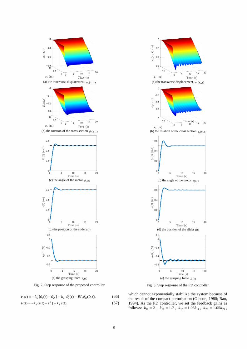
which cannot exponentially stabilize the system because of the result of the compact perturbation (Gibson, 1980; Rao, 1994). As the PD controller, we set the feedback gains as follows: 211 =k , 7.121 =k , 1112 05.1 kk = , 2122 05.1 kk = ,

(a) the transverse displacement ),( 11 txw

(b) the rotation of the cross section ),( 11 tx

(c) the angle of the motor )(1 t

(d) the position of the slider )(ts

(e) the grasping force )(1 t

Fig. 2. Step response of the proposed controller

(a) the transverse displacement ),( 11 txw

(b) the rotation of the cross section ),( 11 tx

(c) the angle of the motor )(1 t

(d) the position of the slider )(ts

(e) the grasping force )(1 t

Fig. 3. Step response of the PD controller

10

44 =k , and 3.35 =k . On the other hand, we set the fol-lowing feedback gains for the proposed controller: 211 =k ,

7.121 =k , 1112 05.1 kk = , 2122 05.1 kk = , 44 =k , 3.35 =k , 8.031 =k , 3132 05.1 kk = , and 8.06 =k . Figs. 2 and 3

show the step response of the proposed controller and the PD controller, respectively. In particular, as an example, we show the responses of ),( 11 txw , ),( 11 tx , )(1 t , s(t), and )(1 t in each figure. In the figures, the dotted line shows the desired value of the corresponding value. From the simulation results, we found that the ),( txw ii ,

),( txii , )(ti , s(t), and )(ti converged to the desired value. Here, note that, not counting the sign (plus or mi-nus) of the value, the responses of ),( 22 txw , ),( 22 tx ,

)(2 t , and )(2 t were almost the same as the responses of ),( 11 txw , ),( 11 tx , )(1 t , and )(1 t , respectively. On the other hand, the responses of the PD controller left some vibrations. Thus, we consider the proposed controller worked well in the step response, and had a higher perfor-mance than the PD controller, which could not exponen-tially stabilize the system.

5.2. Disturbance responses

In the next simulation, we confirmed the boundedness of the closed-loop system under the disturbance at the grasped object described in section 4.2. The same feedback gains and physical parameters as in the case of the step re-sponses were used in this simulation. As the disturbance, the settings were that 1.0=d acted 1 s after the start of the simulation:

=

).1( 1.0

)10( 0

t

td (68)

As an example, we show the response of )(1 t in Fig. 4, where we considered the disturbance response of the pro-posed controller of 5.01 −=d , 5.01 =d , and 6.0=ds . In Fig. 4, (a) shows the response of d, and (b) shows the re-sponse of )(1 t with the disturbance. Note that Fig. 2 (e) is the response of )(1 t without the disturbance. In Fig. 4 (b), the dotted line shows the desired grasping force 1d . From Fig. 2 (e), the response of )(1 t without the disturbance had no steady error; on the other hand, from Fig. 4 (b), it may be seen that the response of )(1 t with the disturbance had a steady error, but did not diverge, and we could con-firm the boundedness of )(1 t . Of course, we confirmed the boundedness of the other states of the system, and found that the proposed controller was robust with respect to the disturbance at the grasped object.

Next, we investigated the relationship between the feed-back gains and performance on disturbance response. The solution of the closed-loop system is estimated as (61) when the disturbance acts at the grasped object. The first term of the right-hand side in (61) corresponds to the initial response, and the second term to the disturbance response. To emphasize the disturbance response, we carried out simulations using the same physical parameters and the following disturbance:

(a) Energies in case (i)

(b) Energies in case (ii)

(c) Energies in case (iii)

Fig. 5. Influences of gains in the disturbance response

(a) disturbance

(b) the grasping force )(1 t with the disturbance. The response of

)(1 t without the disturbance is Fig. 2(e).

Fig. 4. Disturbance response of the proposed controller

11

=

).8( 1.0

)80( 0

t

td (69)

As the feedback gains of the proposed controller, we set 0.21 =ik , 7.12 =ik , and 8.03 =ik , for 2 ,1=i , 0.44 =k , 3.35 =k , and 8.06 =k , and we show the simulation results

for the following three cases: case (i) 11k was changed as follows: 8.0 ,2.1 ,6.1 ,0.211 =k , while other gains were not changed; case (ii) 21k was changed as follows:

0.3 ,5.2 ,0.2 ,7.121 =k while other gains were held steady; and case (iii) 31k was changed as follows:

1.0 ,4.0 ,6.0 ,8.031 =k , while other gains were not changed. Here the changing ranges of the gains were set so that

01 iD and 02 D were satisfied. Figs. 5(a), (b), and (c) show the response of the energy

2||||)( HztE = in cases (i), (ii), and (iii), respectively. From Fig. 5(a), it may be seen that the steady error caused by the disturbance was reduced when 11k was large, but the up-per bound of the response increased. Fig. 5(b) shows that the upper bound was small when 21k was large. However, note that we could not set 21k to be too large, because

)(ti was usually obtained by the numerical difference. On

the other hand, the steady error did not change as 21k was changed. Fig. 5(c) shows that the upper bound became small when 31k was small, but became large when 31k was too small, because the small 31k led to large vibration in the response. On the other hand, the steady error did not change as 31k was changed. Here, note that we obtained the same results for the cases in which the other gains were changed; that is, 12k and 4k had the same performance as

11k ; 22k and 5k had the same performance as 21k ; 32k and 6k had the same performance as 31k . These results give the following guidance as to how to adjust the gains to the disturbance at the grasped object: to obtain a small steady error, large ik1 and 4k are required while 01 iD and 02 D are maintained. To obtain a small upper bound, we need a large ik2 and 5k or small ik3 and 6k while maintaining 01 iD and 02 D , and while noting the vibration of the response.

6. Conclusions

In this paper, we considered a cooperative control prob-lem by two one-link flexible Timoshenko arms. To solve the cooperative control problem, we proposed a boundary cooperative controller based on the hybrid PDE-ODE model. The proposed controller has a simple structure, and is thus easy to implement. Further, to obtain exponential stability without the physically impossible condition, we set the design so that the control actuator consisted of the motor and slider, and the effects of force and torque acted at each flexible beam. The exponential stability of the closed-loop system was proven by the frequency domain method. In addition, we investigated the robustness of the proposed controller with respect to the disturbance at the grasped object and the control input. Finally, in numerical simulations, we confirmed that the proposed controller works well for the step and disturbance responses, and the controller has good performance.

In this paper, we considered a fixed contact model be-tween the flexible arm and grasped object. To make the controller more practical, other contact modes, including rolling contact, are desirable, and we plan to propose such a controller for the cooperative control problem using flex-ible Timoshenko arms in future research.

Acknowledgements

This paper was supported in part by JSPS KAKENHI Grand Number 23700143 and by the Major International Joint Research Project of NSFC under grant no 61520106010.

References

Almeida Júnior, D.S., Santos, M.L., & Muñoz Rivera, J.E. (2013). Stability to weakly dissipative Timoshenko systems, Mathe-matical Methods in the Applied Sciences, 36(14), 1965–1976.

d'Andréa-Novel, B., Boustany, F., Conrad, F., & Rao, B.P. (1994). Feedback stabilization of a hybrid PDE-ODE system: Applica-tion to an overhead crane, Math. Control Signals Syst., 7(1), 1-22.

Choi, J.Y., Hong, K.-S., & Yang, K.-J. (2004). Exponential stabi-lization of an axially moving tensioned strip by passive damp-ing and boundary control. J. Vib. Control, 10(5), 661-682.

Curtain, R.F., & Zwart, H.J. (1995). An introduction to infinite-dimensional linear systems theory. Springer-Verlag New York.

Curtain, R., & Zwart, H. (2016). Stabilization of collocated sys-tems by nonlinear boundary control. Systems & Control Let-ters, 96, 11-14.

Dou, H., & Wang, S. (2014). A boundary control for motion syn-chronization of a two-manipulator system with a flexible beam, Automatica, 50(12), 3088–3099.

Endo, T., Matsuno, F., & Kawasaki, H. (2009). Simple boundary cooperative control of two one-link flexible arms for grasping, IEEE Trans. Autom. Control., 54(10), 2470–2476.

Endo, T., Matsuno, F., & Kawasaki, H. (2014). Force Control and Exponential Stabilization of One-Link Flexible Arm, Interna-tional Journal of Control, 87(9), 1794-1807.

Endo, T., Sasaki, M., & Matsuno, F. (2017). Contact-Force Con-trol of a Flexible Timoshenko Arm, IEEE Trans. Autom. Con-trol., 62(2), 1004-1009.

Engel, K.-J., & Nagel, R. (2000). One-Parameter Semigroups for Linear Evolution Equations. Springer-Verlag New York.

Gibson, J.S. (1980). A note on stabilization of infinite dimension-al linear oscillators by compact linear feedback, SIAM J. of Control and Optimization, 18(3), 311–316.

Grobbelaar-Van Dalsen, M. (2010). Uniform stability for the Ti-moshenko beam with tip load, J. Math. Anal. Appl., 361(2), 392–400.

Han, S.M., Benaroya, H., & Wei, T. (1999). Dynamics of trans-versely vibrating beams using four engineering theories. J. Sound Vib., 225(5), 935–988.

Han, Z.J., & Xu, G.Q. (2009). Stabilization and Riesz Basis Property of Two Serially Connected Timoshenko Beams Sys-tem. Z. Angew. Math. Mech., 89(12), 962–980.

Hong, K.-S. (1997). Asymptotic behavior analysis of a coupled time-varying system: Application to adaptive systems. IEEE Trans. Autom. Control, 42(12), 1693-1697.

He, W., Ge, S.S., How, B.V.E., Choo, Y.S., & Hong, K.-S. (2011). Robust adaptive boundary control of a flexible marine riser with vessel dynamics. Automatica, 47(4), 722-732.

He, W., Zhang, S., & Ge, S.S. (2013). Boundary output-feedback stabilization of a Timoshenko beam using disturbance observ-er, IEEE Trans. Ind. Electron., 60(11), 5186–5194.

He, W., Yang, C., Meng, T., & Sun, C. (2016). Distributed con-trol of a class of flexible mechanical systems with global con-straint. International Journal of Control, 89(1), 128-139.

12

Hokayem, P.F., & Spong, M.W. (2006). Bilateral teleoperation: An historical survey, Automatica, 42(12), 2035–2057.

Huang, T.C. (1961). The effect of rotary inertial and of shear de-formation on the frequency and normal mode equations of uni-form beams with simple end conditions. J. Appl. Mech., 28(4), 579–584.

Krstic, M., & Smyshlyaev, A. (2008). Boundary Control of PDEs. SIAM.

Littman, W., & Markus, L. (1988). Stabilization of a hybrid sys-tem of elasticity by feedback boundary damping. Annu. Mat. Pura Appl., 152(1), 281-330.

Liu, Z., & Zheng, S. (1999). Semigroups associated with dissipa-tive systems. Chapman and Hall/CRC.

Luo, Z.H. (1993). Direct strain feedback control of flexible arms: New theoretical and experimental results, IEEE Trans. Autom. Control., 38(11), 1610–1622.

Luo, Z.-H., Guo, B.-Z., & Morgul, O. (1999). Stability and Stabi-lization of Infinite Dimensional Systems with Applications. Springer-Verlag London Limited.

Luo, Z.H., Kitamura, N., & Guo, B.Z. (1995). Shear force feed-back control of flexible robot arms, IEEE Trans. Robot. Auto-mat., 11(5), 760–765.

Matsuno, F., & Hayashi, A. (2000). PDS cooperative control of two one-link flexible arms, Proc. of the 2000 IEEE Int. Conf. Robotics & Automation, San Francisco, CA (pp.1490–1495).

Matsuno, F., Ohno, T., & Orlov, Y.V. (2002). Proportional deriv-ative and strain (PDS) boundary feedback control of a flexible space structure with a closed-loop chain mechanism. Automat-ica, 38(7), 1201-1211.

Morgül, Ö. (1992). Dynamic boundary control of the Timoshen-ko beam. Automatica, 28(6), 1255–1260.

Morita, Y., Matsuno, F., Ikeda, M., Ukai, H., & Kando, H. (2003). PDS cooperative control of two one-link flexible arms consid-ering bending and torsional deformation, Proc. of the 29th Ann. Conf. of the IEEE Industrial Electronics Society, (pp.466–471).

Muñoz Rivera, J.E., & Ávila, A.I. (2015). Rates of decay to non homogeneous Timoshenko model with tip body, J. Differen-tial Equations, 258(10), 3468–3490.

Murray, R.M., Li, Z., & Sastry, S.S. (1994). A Mathematical In-troduction to Robotic Manipulation. CRC Press LLC.

Nguyen, Q.C., & Hong, K.-S. (2010). Asymptotic stabilization of a nonlinear axially moving string by adaptive boundary con-trol. J. Sound Vib., 329(22), 4588-4603.

Pazy, A. (1983). Semigroups of linear operators and applications to partial differential equations. Springer-Verlag New York.

Rao, B. (1994). Recent progress in non-uniform and uniform sta-bilization of the SCOLE model with boundary feedbacks. In J. P. Zolésio (ed.), Bounday control and variation (pp.357–365), Marcel Dekker New York.

Slemrod, M., (1989). Feedback stabilization of a linear control system in Hilbert space with an a priori bounded control, Math. Control Signals Syst., 2(3), 265-285.

Soufyane, A., & Wehbe, A. (2003). Uniform stabilization for the Timoshenko beam by a locally distributed damping, Electron. J. Differential Equations, 29, 1–14.

Taylor, S.W., & Yau, S.C.B. (2003). Boundary control of a rotat-ing Timoshenko beam, J. ANZIAM, 44, E143–E184.

Yang, K.-J., Hong, K.-S., & Matsuno, F. (2005). Boundary con-trol of a translating tensioned beam with varying speed. IEEE/ASME Trans. Mechatronics, 10(5), 594-597.

Yoshikawa, T. (2000). Force control of robot manipulators. Proc. of the 2000 IEEE Int. Conf. Robotics & Automation, San Fran-cisco, CA (pp.220–226).

Zhang, F., Dawson, D.M., de Queiroz, M.S., & Vedagarbha, P. (1997). Boundary control of the Timoshenko beam with free-end mass/inertial dynamics. Proc. of the 36th IEEE Conf. on Decision and Control, San Diego, CA (pp.245–250).

Appendix A. Proof of estimate (33)

We prove estimate (33). From the equation

+=ix

ijijiij ussuxu0

)0(d)()( , the Cauchy-Schwartz inequality, and (36), we obtain

,)0( } {22

1

2

22 ijL

ijL

ij uuu + (A.1)

where 1 is a positive constant. On the other hand, inte-grating the equation

2

112

2

2

2

12 )Re(2 iiiiii uuuuuu +−=− and using the inequality /2

22baba + for C , ba ,

+R , gives

.)/11()1(2

1

2

2

2

12 222 LiLiLii uuuu −+−− (A.2)

Thus, we obtain the following using (A.1) and (A.2): for ),0(),0(),( 11

21 lHlHuu ii

,)1

1(44

)1(2

)1

1(4

4})0({

)1(2

})0({

)0(4

)0(2

)1

1(2

)1(22

),(

2

1

2

2

2

1

1

32

2

1

2

2

1

2

2

2

1

2

13

2

2

2

2

2

22

2

142

212

1

2

2

2

2

2

121

22

22

2

22

22

2

22

Lii

Lii

LiLii

Lii

Lii

iLi

Lii

iLi

iii

Lii

Lii

Lii

ii

uK

uEI

uuK

uK

uEI

uu

uK

uu

uk

uk

uK

uK

uEI

uu

−++

+

−+

−+

+++

−++

++−+

−+

(A.3)

where }2/,4/min{ 12 ii kEI= , and }4/,4/)/11(min{ 43 kKi −= .

Here, if we set 1)/(21 12 + iK , we can obtain the posi-

tive constant 4 satisfying

.),(),(2

2214

2

121 iiii uuuu (A.4)

Here, (A.4) means the estimate (33).