Tire-Road Friction, Drag Factor and Deceleration

Rudy Limpert and Dennis Andrews

www.pcbrakeinc.com

Short Paper PCB 1-2012

Introduction

Many years ago when SAE International sold our reconstruction software LARM2 software,

I received a phone call from a Reconstructionist who had bought the program. He stated that he

was very disappointed that LARM2 did not provide any drag factors for vehicles after impact.

When I asked him what the case was all about, he did not know – he just needed the numbers.

When I told him that the after-impact drag factor depends on the run-out dynamics including

information on wheel(s) locked, terrain, grade, secondary energy such as impact with trees,

rolling resistance, drag sled factor, skid tests, etc. he was surprised.

After-impact decelerations are of critical importance when calculating impact speeds. They

are used to compute speeds immediately after impact, which then are used in the impulse

analysis to compute speeds immediately before impact. Before-impact decelerations are

extremely critical for travel speed calculations and causation and accident avoidance analysis.

Basic Physics

Only the fundamentals are reviewed here. Vehicle Motion Analysis is discussed in “Motor

Vehicle Accident Reconstruction and Cause Analysis”, 7th

edition by Rudolf Limpert, 2012,

LexisNexis Publisher. The MARC1 software programs discussed in this paper are available from

www.pcbrakeinc.com as a fully functioning no-charge MARC1-2013 download.

A vehicle slows its speed when it decelerates. Deceleration is velocity change or decrease

divided by the time period during which the vehicle decelerates.

Deceleration a = (V2 –V1) / (t2 -t1); ft/sec2

Subscript 1 designates beginning of braking, subscript 2 end of braking. No matter, what terms

are used, a vehicle slows only when its velocity measured in ft/sec changes its value per unit

time, measured in seconds. When coming to a complete stop and assuming deceleration is

constant, the distance is

Stopping Distance S = V2/(2a); ft

Deceleration a is measured in ft/sec2, velocity V in ft/sec.

Many motion equations use these two terms and other coherent measuring units. Coherent

units means that the left side of the equation {feet} relates directly in a one-to-one relationship to

the right side of the equation {(ft/sec)2/(ft/sec

2) = feet} However, for short-term convenience

stopping distance equations are often used where velocity is measured in miles per hour,

deceleration in g-units, and distance in feet, resulting in incoherent equations. An example of a

popular and widely used incoherent equation is S = V2/(30f) where velocity V is measured in

mph, f in g-units and distance S in ft. The number 30 is a conversion number deriving from using

an incoherent mixture of units. See page 20-41 of the 7th

edition for derivation details. Matters

become confusing when concepts are used where coherent units must be used such as in energy

balance which is measured in lbft.

Case 1: The Accident Scene

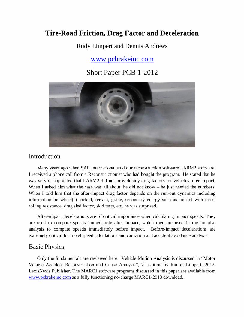
We will discuss an actual accident illustrated below in the police scene photograph. A

pickup truck impacted a boy riding a bicycle. The bike came from the right side of the truck with

the truck traveling south.

The left front tire skidded approximately 88 feet, the right front 86 feet. No rear tire skid marks

were observed at the scene. The bike was impacted by the left front corner of the truck

approximately 9 feet before the truck came to rest. The legal speed limit was 30 mph. The truck

had the legal right-of-way. The rider of the bike was a young 7-year old boy.

Inspection of the accident scene photographs clearly show the front tire skid marks with darker

tread edge markings of the right front tire. The tire marks continued to the rest position of the

truck’s front tires. No rear tire skid marks were shown in any of the photographs.

An inspection of the 1982 Dodge flatbed pickup truck showed that one rear brake was leaking

thus not producing any rear braking force. The static front and rear axle loads and wheel base

were measured, the empty center-of-gravity height estimated.

Dodge – Bicycle Accident Scene.

We must compute the most probable speed of the truck at the beginning of skid marks, the travel

speed, the impact speed against the bike, and perform an accident avoidance analysis. To do that,

we must determine the probable deceleration or drag factor of the subject truck at the time of the

accident.

Case 1: Dodge Accident Site Tire Road Friction Coefficient

At the time of our accident site inspection, no case-specific tire marks were visible. The

truck was not available for skid measurements. Consequently, our first job is to determine the

“stickiness” of the accident site where the skid marks were measured by the police. It is

important to make any tire-road friction coefficient measurements under conditions similar to

those existing at the time of the accident. Using a common drag boot frequently employed by

investigating officers and experts yielded the following: an average drag force of 37 lb in five

tests for a drag boot weight of 50 lb resulted in an average drag boot factor of 37/50 = 0.74. All

we have accomplished thus far is giving the road a name in terms of a 0.74 drag boot factor

existing at the time of our inspection. This number does not tell us anything about the

deceleration the truck actually experienced at the time of the crash. However, in many cases the

“stickiness name” of the road measured with a drag boot is all we have to start with!

At the accident site we also used a pickup truck to conduct maximum braking effectiveness

stops from a speed of 35 mph using a G-analyst resulting in an average deceleration of 0.84g in

five skid tests. In each test the ABS system began to modulate on all four brakes. Now we have

given the accident site an additional name indicating an average deceleration of 0.84g with all

four brakes ABS modulating with our truck tires.

What tire-road friction coefficient the braked tires of the subject truck experienced depends

upon how our truck tires compare to the subject tires, and how much difference exists between a

locked tire (Dodge) and peak friction tire (our truck). However, we safely assume that it is larger

than the drag boot and lower than the ABS value. Braking force/slip (slip)curves typically

show little difference between peak and sliding friction for dry roadways (Figure 22-3 of 7th

edition). Consequently, we assign a tire-road friction coefficient of fsite = (0.74 + 0.84)/2 = 0.79

to the subject road at the time of the accident. Consequently, assuming no other case-specific

data become available, we must support and defend in court an accident-site specific tire-road

friction coefficient of 0.79. As we will see from the speed analysis, in this particular case an

accurate probable drag factor is more important than if the skid mark length had been 200 feet

instead of only 88 feet.

Comparing the measured tire road friction coefficient of 0.79 to typical values published in

the literature shows ranges 0.65 – 0.9 for sliding and 0.80 to 1.00 for peak friction on

concrete/asphalt, polished to new, dry (Table 22-3 of 7th edition).

If the Dodge accident had occurred on wet pavement, the likelihood of obtaining any

meaningful specific pavement “stickiness” data would have been very small. The friction of the

Dodge tires depend upon water depth, tread design, vehicle speed, etc. See Chapter 22 of the 7th

Edition for details. State highway departments regularly measure wet skid resistance of major

highways for inventory and statistical analysis. Bridge pavement friction data are frequently not

measured. Test method and equipment are covered by standard ASTM E 274 (American

Society of Testing and Materials). The test tires to be used with the skid trailer are specified

ribbed (treaded) in ASTM E 501, and smooth (bald) in ASTM E 524. From a reconstruction

view point, these numbers only give a particular highway a “ wet friction” name and may not

indicate what the wet friction of a specific subject tire may have been. However, depending upon

the accident, it may be an additional or only data source and a place to start.

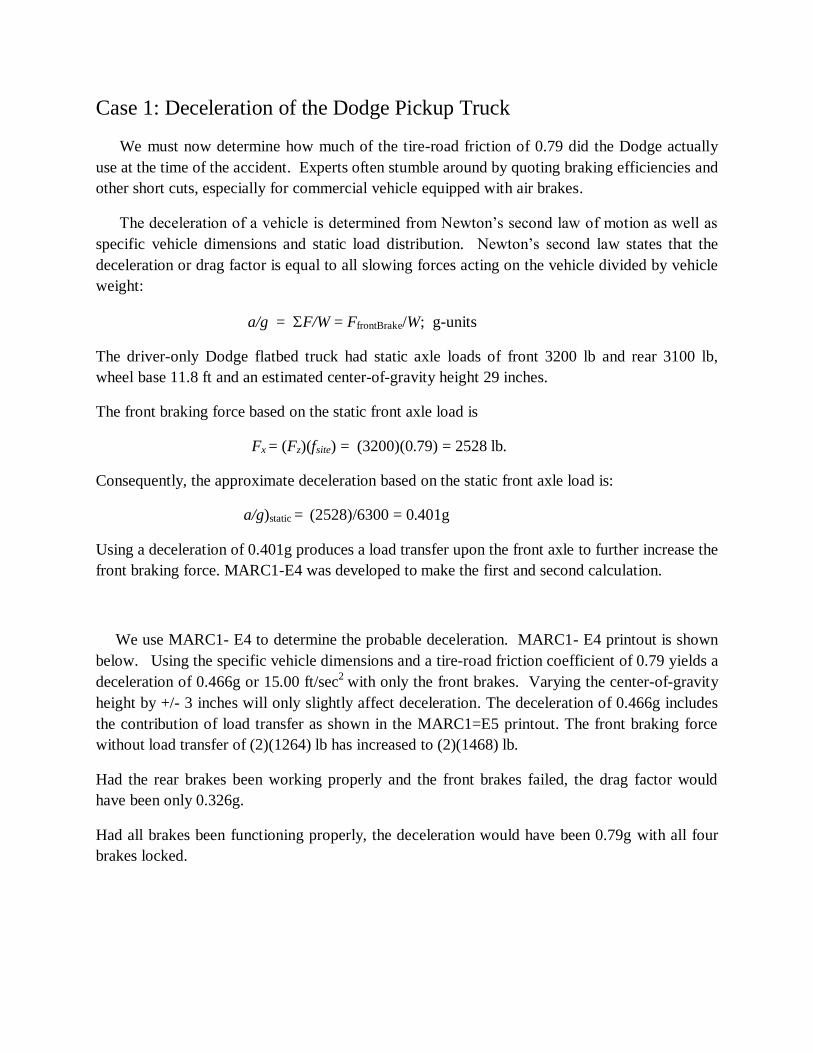
Case 1: Deceleration of the Dodge Pickup Truck

We must now determine how much of the tire-road friction of 0.79 did the Dodge actually

use at the time of the accident. Experts often stumble around by quoting braking efficiencies and

other short cuts, especially for commercial vehicle equipped with air brakes.

The deceleration of a vehicle is determined from Newton’s second law of motion as well as

specific vehicle dimensions and static load distribution. Newton’s second law states that the

deceleration or drag factor is equal to all slowing forces acting on the vehicle divided by vehicle

weight:

a/g = F/W = FfrontBrake/W; g-units

The driver-only Dodge flatbed truck had static axle loads of front 3200 lb and rear 3100 lb,

wheel base 11.8 ft and an estimated center-of-gravity height 29 inches.

The front braking force based on the static front axle load is

Fx = (Fz)(fsite) = (3200)(0.79) = 2528 lb.

Consequently, the approximate deceleration based on the static front axle load is:

a/g)static = (2528)/6300 = 0.401g

Using a deceleration of 0.401g produces a load transfer upon the front axle to further increase the

front braking force. MARC1-E4 was developed to make the first and second calculation.

We use MARC1- E4 to determine the probable deceleration. MARC1- E4 printout is shown

below. Using the specific vehicle dimensions and a tire-road friction coefficient of 0.79 yields a

deceleration of 0.466g or 15.00 ft/sec2

with only the front brakes. Varying the center-of-gravity

height by +/- 3 inches will only slightly affect deceleration. The deceleration of 0.466g includes

the contribution of load transfer as shown in the MARC1=E5 printout. The front braking force

without load transfer of (2)(1264) lb has increased to (2)(1468) lb.

Had the rear brakes been working properly and the front brakes failed, the drag factor would

have been only 0.326g.

Had all brakes been functioning properly, the deceleration would have been 0.79g with all four

brakes locked.

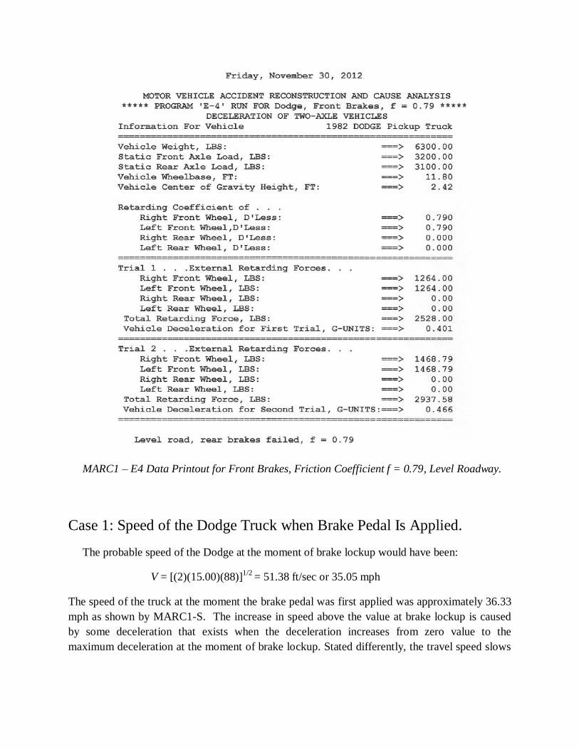
MARC1 – E4 Data Printout for Front Brakes, Friction Coefficient f = 0.79, Level Roadway.

Case 1: Speed of the Dodge Truck when Brake Pedal Is Applied.

The probable speed of the Dodge at the moment of brake lockup would have been:

V = [(2)(15.00)(88)]1/2

= 51.38 ft/sec or 35.05 mph

The speed of the truck at the moment the brake pedal was first applied was approximately 36.33

mph as shown by MARC1-S. The increase in speed above the value at brake lockup is caused

by some deceleration that exists when the deceleration increases from zero value to the

maximum deceleration at the moment of brake lockup. Stated differently, the travel speed slows

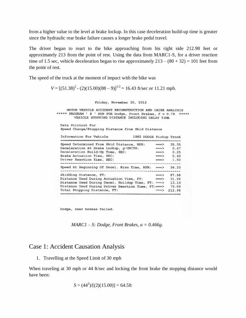
from a higher value to the level at brake lockup. In this case deceleration build-up time is greater

since the hydraulic rear brake failure causes a longer brake pedal travel.

The driver began to react to the bike approaching from his right side 212.98 feet or

approximately 213 from the point of rest. Using the data from MARC1-S, for a driver reaction

time of 1.5 sec, vehicle deceleration began to rise approximately 213 – (80 + 32) = 101 feet from

the point of rest.

The speed of the truck at the moment of impact with the bike was

V = [(51.38)2 - (2)(15.00)(88 – 9)]

1/2 = 16.43 ft/sec or 11.21 mph.

MARC1 – S: Dodge, Front Brakes, a = 0.466g.

Case 1: Accident Causation Analysis

1. Travelling at the Speed Limit of 30 mph

When traveling at 30 mph or 44 ft/sec and locking the front brake the stopping distance would

have been:

S = (442)/[(2)(15.00)] = 64.5ft

Consequently, had the driver driven at the speed limit of 30 mph and locked the front brakes at

the same location as in the accident, the truck would have stopped approximately 88 – 9 – 64.5 =

14.5 ft from POI.

2. Traveling at 36.33 mph with Good Brakes

With good brakes and all brakes locked the deceleration would have been (0.79)(32.2) = 25.44

ft/sec2. The drag factor is 0.79g. The speed is (36.33)(1.466) = 53.26 ft/sec. The stopping

distance would have been:

S = (53.262)/[(2)(25.44))] = 55.75 ft.

Consequently, the truck would have stopped 88 – 9 – 55.75 = 23.25 ft from POI.

The case settled due to excessive speed and defective safety inspection.

Case 1: Assume the Dodge Accident Site Had a 7-degree Downslope

A slope angle = 7 degrees equals a slope 12.2%, since tan7 = 0.122.

The tire forces between ground and Dodge change. See Case 3 for details. The vertical weight

force becomes Wcos, and the downhill gravity force becomes Wsin. The downhill force will

do two things, namely place more weight onto the front axle due to weight transfer similar to the

regular load transfer due to braking as well as it forces the Dodge move downhill. The MARC1

– E5 is shown below. The deceleration now becomes 0.344g or 11.08 ft/sec2. The probable

speed at begin of skidding with a drag factor of 0.344 would have been 30 mph instead of 35.2

mph on the level road with a drag factor of 0.466g.

Using any simplified method of subtracting the slope from the level deceleration such as 0.47 –

0.12 = 0.35g, a slightly larger value than 0.344g.

MARC1 – E5 Data Printout for Front Brakes on Slope of 7 Degrees. Downhill Braking.

If the rear brakes had been functioning properly and the front brakes failed, the drag factor would

have been only 0.205g indicating that on a downhill slope the rear brakes are not as effective as

the front brakes. On a seven-degree uphill grade the rear brakes-only drag factor would have

been 0.442g

If the rear brakes had also been locked, then the deceleration would have been 0.662g as shown

in the MARC1-E5 below. The approximate downhill drag factor would have been 0.79 – 0.12 =

0.67g.

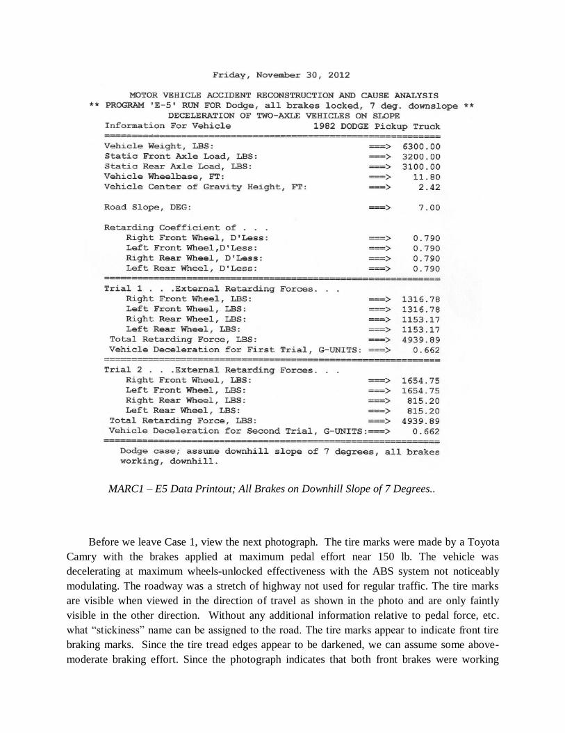
MARC1 – E5 Data Printout; All Brakes on Downhill Slope of 7 Degrees..

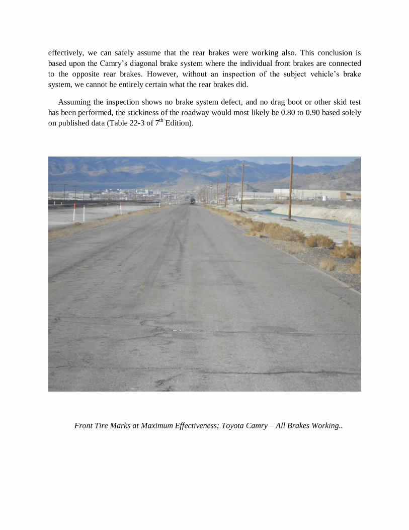
Before we leave Case 1, view the next photograph. The tire marks were made by a Toyota

Camry with the brakes applied at maximum pedal effort near 150 lb. The vehicle was

decelerating at maximum wheels-unlocked effectiveness with the ABS system not noticeably

modulating. The roadway was a stretch of highway not used for regular traffic. The tire marks

are visible when viewed in the direction of travel as shown in the photo and are only faintly

visible in the other direction. Without any additional information relative to pedal force, etc.

what “stickiness” name can be assigned to the road. The tire marks appear to indicate front tire

braking marks. Since the tire tread edges appear to be darkened, we can assume some above-

moderate braking effort. Since the photograph indicates that both front brakes were working

effectively, we can safely assume that the rear brakes were working also. This conclusion is

based upon the Camry’s diagonal brake system where the individual front brakes are connected

to the opposite rear brakes. However, without an inspection of the subject vehicle’s brake

system, we cannot be entirely certain what the rear brakes did.

Assuming the inspection shows no brake system defect, and no drag boot or other skid test

has been performed, the stickiness of the roadway would most likely be 0.80 to 0.90 based solely

on published data (Table 22-3 of 7th Edition).

Front Tire Marks at Maximum Effectiveness; Toyota Camry – All Brakes Working..

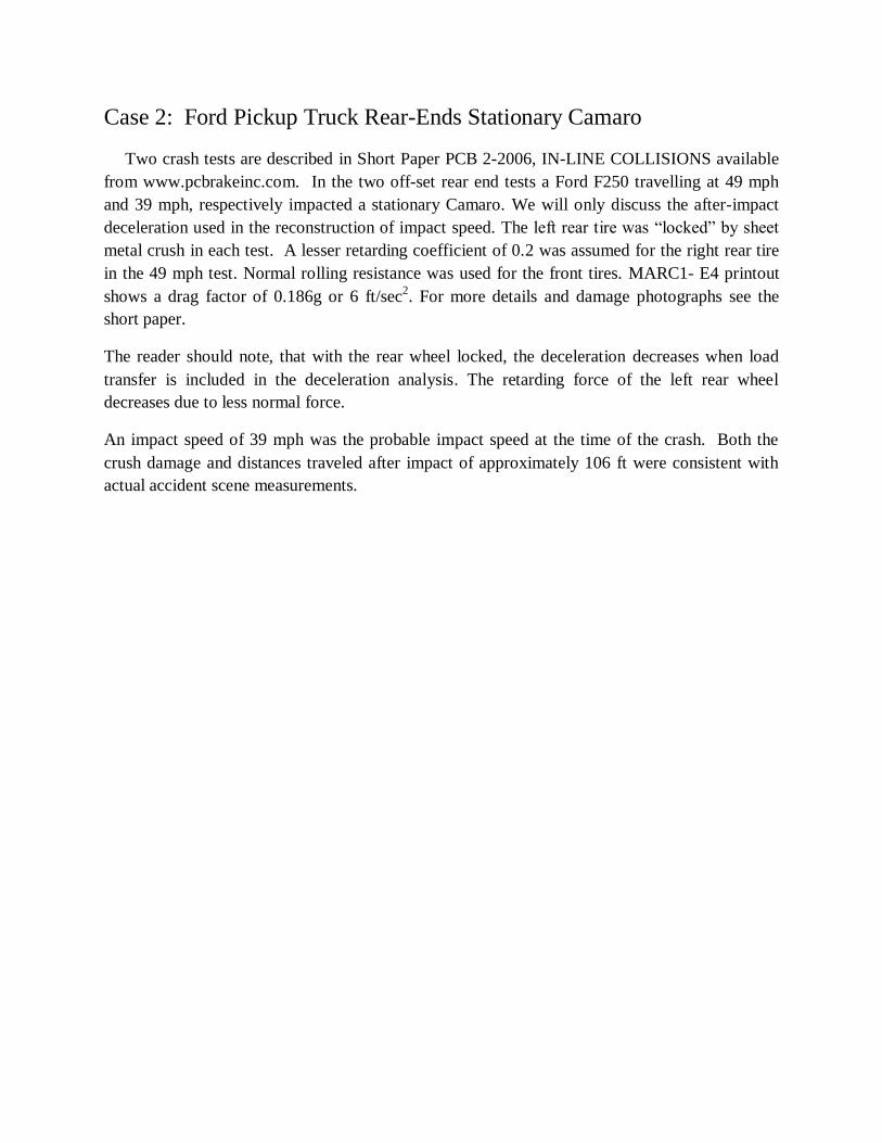
Case 2: Ford Pickup Truck Rear-Ends Stationary Camaro

Two crash tests are described in Short Paper PCB 2-2006, IN-LINE COLLISIONS available

from www.pcbrakeinc.com. In the two off-set rear end tests a Ford F250 travelling at 49 mph

and 39 mph, respectively impacted a stationary Camaro. We will only discuss the after-impact

deceleration used in the reconstruction of impact speed. The left rear tire was “locked” by sheet

metal crush in each test. A lesser retarding coefficient of 0.2 was assumed for the right rear tire

in the 49 mph test. Normal rolling resistance was used for the front tires. MARC1- E4 printout

shows a drag factor of 0.186g or 6 ft/sec2. For more details and damage photographs see the

short paper.

The reader should note, that with the rear wheel locked, the deceleration decreases when load

transfer is included in the deceleration analysis. The retarding force of the left rear wheel

decreases due to less normal force.

An impact speed of 39 mph was the probable impact speed at the time of the crash. Both the

crush damage and distances traveled after impact of approximately 106 ft were consistent with

actual accident scene measurements.

MARC1 – E4 Data Printout Ford/Camaro 49 mph Test, a = 0.19g.

Case 3: Sliding Up- or Downhill with all Brakes Locked

The prevailing wisdom in the accident reconstruction community is to simply add or subtract

the grade from the level road tire-road friction coefficient. We must realize that this approach is

only valid for small slope angles.

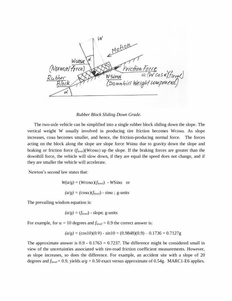
Rubber Block Sliding Down Grade.

The two-axle vehicle can be simplified into a single rubber block sliding down the slope. The

vertical weight W usually involved in producing tire friction becomes WcosAs slope

increases, cosbecomes smaller, and hence, the friction-producing normal force. The forces

acting on the block along the slope are slope force Wsin due to gravity down the slope and

braking or friction force (flevel)(Wcosup the slope. If the braking forces are greater than the

downhill force, the vehicle will slow down, if they are equal the speed does not change, and if

they are smaller the vehicle will accelerate.

Newton’s second law states that:

W(a/g) = (Wcosflevel) - WSinor

(a/g) = (cosflevel)- sing-units

The prevailing wisdom equation is:

(a/g) = flevel)- slopeg-units

For example, for = 10 degrees and flevel = 0.9 the correct answer is:

(a/g) = (cos10)- sin10 = (0.9848)(0.9) – 0.1736 = 0.7127g

The approximate answer is 0.9 - 0.1763 = 0.7237. The difference might be considered small in

view of the uncertainties associated with tire-road friction coefficient measurements. However,

as slope increases, so does the difference. For example, an accident site with a slope of 20

degrees and flevel = 0.9, yields a/g = 0.50 exact versus approximate of 0.54g. MARC1-E6 applies.

As slope increases a critical level will be reached when friction force and downhill gravity

force balance. At that point the vehicle will neither accelerate nor decelerate down-hill. The

critical slope is reached whenflevel)= tanOf course, this is the equation we implemented in

high school physics many years ago when measuring the friction coefficient of different mating

surfaces by raising a hinged slope with an angle measuring device. Once the body began to slide,

we read the slope angle and taking tan we knew the static friction coefficient.

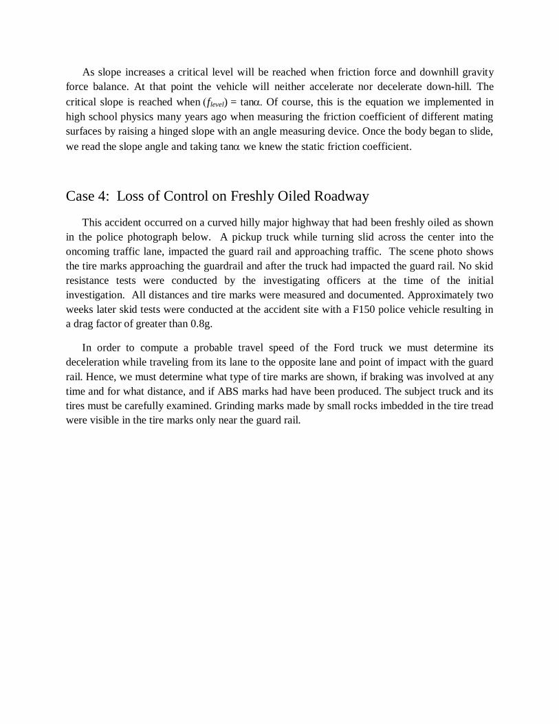
Case 4: Loss of Control on Freshly Oiled Roadway

This accident occurred on a curved hilly major highway that had been freshly oiled as shown

in the police photograph below. A pickup truck while turning slid across the center into the

oncoming traffic lane, impacted the guard rail and approaching traffic. The scene photo shows

the tire marks approaching the guardrail and after the truck had impacted the guard rail. No skid

resistance tests were conducted by the investigating officers at the time of the initial

investigation. All distances and tire marks were measured and documented. Approximately two

weeks later skid tests were conducted at the accident site with a F150 police vehicle resulting in

a drag factor of greater than 0.8g.

In order to compute a probable travel speed of the Ford truck we must determine its

deceleration while traveling from its lane to the opposite lane and point of impact with the guard

rail. Hence, we must determine what type of tire marks are shown, if braking was involved at any

time and for what distance, and if ABS marks had have been produced. The subject truck and its

tires must be carefully examined. Grinding marks made by small rocks imbedded in the tire tread

were visible in the tire marks only near the guard rail.

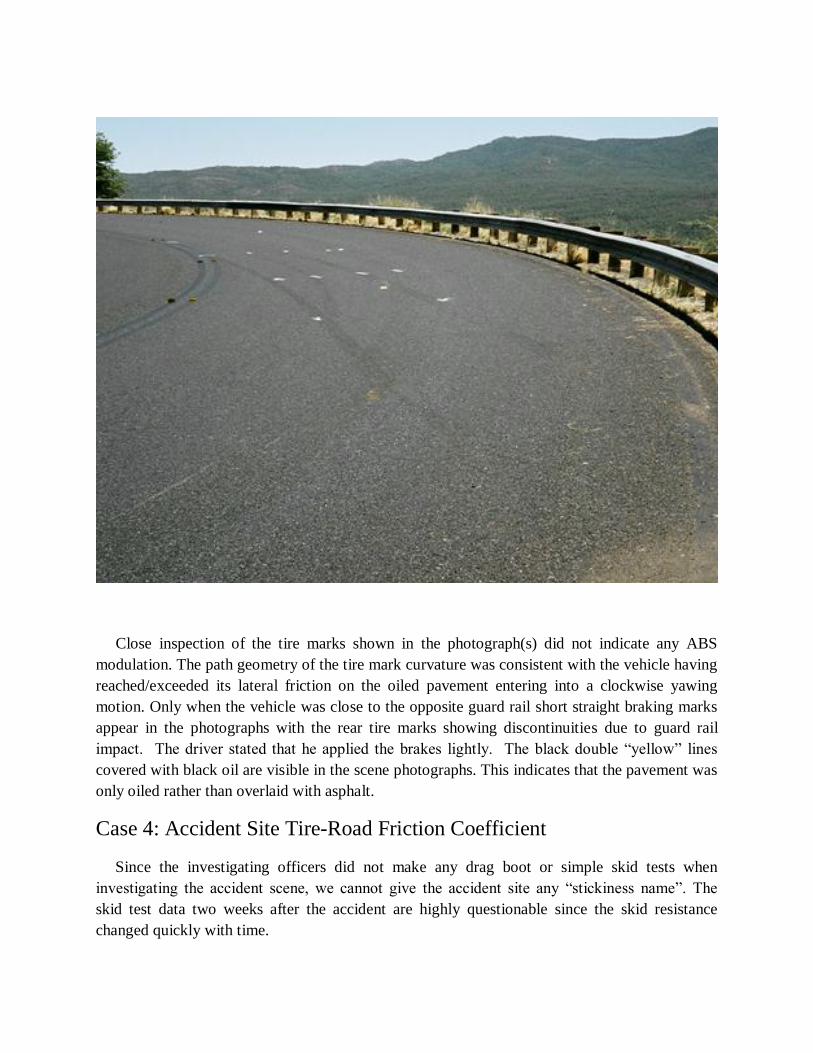
Close inspection of the tire marks shown in the photograph(s) did not indicate any ABS

modulation. The path geometry of the tire mark curvature was consistent with the vehicle having

reached/exceeded its lateral friction on the oiled pavement entering into a clockwise yawing

motion. Only when the vehicle was close to the opposite guard rail short straight braking marks

appear in the photographs with the rear tire marks showing discontinuities due to guard rail

impact. The driver stated that he applied the brakes lightly. The black double “yellow” lines

covered with black oil are visible in the scene photographs. This indicates that the pavement was

only oiled rather than overlaid with asphalt.

Case 4: Accident Site Tire-Road Friction Coefficient

Since the investigating officers did not make any drag boot or simple skid tests when

investigating the accident scene, we cannot give the accident site any “stickiness name”. The

skid test data two weeks after the accident are highly questionable since the skid resistance

changed quickly with time.

At this time of the investigation and data collection process by the expert/consultant it

becomes critical to review all witness statements with respect to any observations they may have

made of the slipperiness of the road at the time of the accident. Other accidents, if any, which

may have occurred on the freshly oiled highway must be investigated. We also know that for

wet road conditions the tire-road friction coefficient is approximately 0.55 for the average road

and tire tread. In the absence of an over-involvement of wet road accidents at the accident

highway, we may conclude that the tire-road friction coefficient at the time of the crash was less

than 0.55. Diesel fuel spilled on wet pavement has a friction coefficient of 0.35 or less. Taking

the average of both values yields a drag factor of 0.45g.

A careful review of published research literature may assist in obtaining accepted drag

factors of freshly oiled pavements.

Case 4: Speed Analysis

We have two concepts of physics that may be employed for speed calculation, namely

sustainable limit speed in a curve without slide-out, or speed from skid resistance and skidding

distance. For each method the drag factor of the subject truck at the time of the accident must be

known. To compute the limit turning speed the road curvature or radius must be measured. For a

radius of 260 ft the limit turning speed is approximately 39 to 42 mph when using a limit lateral

acceleration of 0.4 to 0.45g. Using a travel speed of 40 mph would indicate an average braking

deceleration of approximately 0.2g over a distance of 280 ft. The braking effort is consistent

with the driver statement. If the truck traveled 15 mph when impacting the guard rail based upon

crush damage, the truck traveled approximately 43 mph before beginning to slide.

Human factors studies measuring lateral accelerations in regular highway traffic curves

indicate that drivers tend to utilize approximately 0.45g at a speed of 30 mph and still “feel safe”.

At higher speeds the lateral accelerations decrease to approximately 0.1g at 70 mph (See page

31-6 of 7th edition).

Conclusions

1. Give the accident scene/site a “stickiness” name providing a place to start for the speed

analysis. Doing this is of particular importance when dealing with non-typical surfaces

such as median, gravel, wet, snow, oils or Diesel fuel spills, muddy construction zones,

oiled pavements, etc. Having measured some accident scene data points and analyze

them is better than to have measured nothing and trying “analyze” that.

2. As a minimum, use a drag boot for item 1 or similar device.

3. If possible, use subject vehicle or other vehicle for skid/ABS testing at accident scene.

4. Interpret accident scene tire marks correctly. If not certain, run both ABS and skid tests.

5. Inspect subject vehicle(s) for any brake system defects.

6. Determine if subject vehicle had ABS actuation from tire marks, and data recorder.

7. Inspect subject tires for any traction force affecting conditions. Measure inflation

pressure. Note tread depths and unusual wear patterns.

8. Use proper method to determine, if possible, probable drag factor or deceleration of

subject vehicle at time of accident from original “stickiness” data.

9. Check your drag factor results against published data generally accepted by

reconstruction community.

10. For slope angles less than 10 degrees the “prevailing wisdom” equation may be used,

meaning you can subtract the downhill slope as fraction (percent x 100) from the drag

factor the subject vehicle would have experienced on a level road. Do the opposite for an

uphill slope.

11. Compute probable vehicle speed(s) using a reasonable data range.

12. Use the DIMS or Does It Make Sense check of your data against any other case specific

data such as crush damage, witness statements, view analysis, etc.