Embed Size (px)
Citation preview
E n e r g y R e s e a r c h a n d D e v e l o p m e n t D i v i s i o n F I N A L P R O J E C T R E P O R T
TIME OF USE WATER METER IMPACTS ON CUSTOMER WATER USE
OCTOBE R 2010 CE C-500-2013-146
Prepared for: California Energy Commission Prepared by: Water and Energy Consulting
PREPARED BY: Primary Author(s): Lon House Water and Energy Consulting Cameron Park, CA 95682 Contract Number: 500-07-022 Prepared for: California Energy Commission Richard Sapuda Contract Manager Virginia Lew Office Manager Energy Efficiency Research Office Laurie ten Hope Deputy Director ENERGY RESEARCH AND DEVELOPMENT DIVISION Robert P. Oglesby Executive Director
DISCLAIMER This report was prepared as the result of work sponsored by the California Energy Commission. It does not necessarily represent the views of the Energy Commission, its employees or the State of California. The Energy Commission, the State of California, its employees, contractors and subcontractors make no warranty, express or implied, and assume no legal liability for the information in this report; nor does any party represent that the uses of this information will not infringe upon privately owned rights. This report has not been approved or disapproved by the California Energy Commission nor has the California Energy Commission passed upon the accuracy or adequacy of the information in this report.

ACKNOWLEDGEMENTS
This work funded by the California Energy Commission (Energy Commission), Public Interest Energy Research (PIER) Program, under Contract No. 500-07-022.
The author wishes to thank the members of the Program Advisory Committee for their guidance, assistance, and their review of this document:
Aquacraft – Bill DeOreo;
Association of California Water Agencies (ACWA) Washington representative – Dr. Abbey Schneider;
California Department of Water Resources – Dave Todd;
California Energy Commission –Mike Gravely and Shahid Chaundry;
California Public Utilities Commission – Ted Howard, Mikhail Haramati, and Katherine Hardy;
California Urban Water Conservation Council – Chris Brown;
Electric Power Research Institute – Mark McGrangham;
EnerNoc – James McPhail;
Lawrence Berkeley National Laboratory – Larry Dale;
Master Meter - Ed Amelung;
Southern California Edison Company – Matt Garcia, Curtis DeWoody, and James Pasmore;
Water Research Foundation – Maureen Hodgins and Linda Reekie;
Water Utilities:
Glendale Water and Power – Peter Kavounas; Valencia Water Company – Robert DiPrino; Tehachapi Cummins Water District – John Otto
i

PREFACE
The California Energy Commission Energy Research and Development Division supports public interest energy research and development that will help improve the quality of life in California by bringing environmentally safe, affordable, and reliable energy services and products to the marketplace.
The Energy Research and Development Division conducts public interest research, development, and demonstration (RD&D) projects to benefit California.
The Energy Research and Development Division strives to conduct the most promising public interest energy research by partnering with RD&D entities, including individuals, businesses, utilities, and public or private research institutions.
Energy Research and Development Division funding efforts are focused on the following RD&D program areas:
• Buildings End-Use Energy Efficiency
• Energy Innovations Small Grants
• Energy-Related Environmental Research
• Energy Systems Integration
• Environmentally Preferred Advanced Generation
• Industrial/Agricultural/Water End-Use Energy Efficiency
• Renewable Energy Technologies
• Transportation
Time-of-Use Water Meter Impacts on Customer Water Use is the final report for the Time of Use Water Meter Technology project (contract number 500-07-022) conducted by Water and Energy Consulting. The information from this project contributes to Energy Research and Development Division’s Energy Systems Integration Program.
For more information about the Energy Research and Development Division, please visit the Energy Commission’s website at www.energy.ca.gov/research/ or contact the Energy Commission at 916-327-1551.
ii
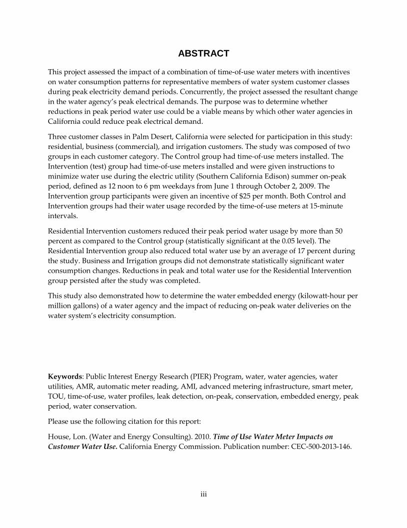
ABSTRACT
This project assessed the impact of a combination of time-of-use water meters with incentives on water consumption patterns for representative members of water system customer classes during peak electricity demand periods. Concurrently, the project assessed the resultant change in the water agency’s peak electrical demands. The purpose was to determine whether reductions in peak period water use could be a viable means by which other water agencies in California could reduce peak electrical demand.
Three customer classes in Palm Desert, California were selected for participation in this study: residential, business (commercial), and irrigation customers. The study was composed of two groups in each customer category. The Control group had time-of-use meters installed. The Intervention (test) group had time-of-use meters installed and were given instructions to minimize water use during the electric utility (Southern California Edison) summer on-peak period, defined as 12 noon to 6 pm weekdays from June 1 through October 2, 2009. The Intervention group participants were given an incentive of $25 per month. Both Control and Intervention groups had their water usage recorded by the time-of-use meters at 15-minute intervals.
Residential Intervention customers reduced their peak period water usage by more than 50 percent as compared to the Control group (statistically significant at the 0.05 level). The Residential Intervention group also reduced total water use by an average of 17 percent during the study. Business and Irrigation groups did not demonstrate statistically significant water consumption changes. Reductions in peak and total water use for the Residential Intervention group persisted after the study was completed.
This study also demonstrated how to determine the water embedded energy (kilowatt-hour per million gallons) of a water agency and the impact of reducing on-peak water deliveries on the water system’s electricity consumption.
Keywords: Public Interest Energy Research (PIER) Program, water, water agencies, water utilities, AMR, automatic meter reading, AMI, advanced metering infrastructure, smart meter, TOU, time-of-use, water profiles, leak detection, on-peak, conservation, embedded energy, peak period, water conservation.
Please use the following citation for this report:
House, Lon. (Water and Energy Consulting). 2010. Time of Use Water Meter Impacts on Customer Water Use. California Energy Commission. Publication number: CEC-500-2013-146.
iii

TABLE OF CONTENTS
Acknowledgements ................................................................................................................................... i
PREFACE ................................................................................................................................................... ii
ABSTRACT .............................................................................................................................................. iii
TABLE OF CONTENTS ......................................................................................................................... iv
LIST OF FIGURES .................................................................................................................................... v
LIST OF TABLES .................................................................................................................................... vi
EXECUTIVE SUMMARY ........................................................................................................................ 1
Introduction ........................................................................................................................................ 1
Project Purpose ................................................................................................................................... 1
Project Results ..................................................................................................................................... 1
Project Benefits ................................................................................................................................... 2
CHAPTER 1: Introduction ...................................................................................................................... 3
CHAPTER 2: Project Approach .............................................................................................................. 4
2.1 Background ................................................................................................................................. 4
2.2 Meter Requirements .................................................................................................................. 5
2.3 Data and Statistical Analysis .................................................................................................... 6
CHAPTER 3: Project Results .................................................................................................................. 9
3.1 Representativeness of Study Participants .............................................................................. 9
3.2 Leak Detection .......................................................................................................................... 12
3.2.1 Residential Group ................................................................................................................... 14
3.2.2 Irrigation Group ...................................................................................................................... 14
3.2.3 Business Group ........................................................................................................................ 14
3.3 Water Usage - Hourly ............................................................................................................. 14
3.3.1 Residential ................................................................................................................................ 14
3.3.2 Irrigation ................................................................................................................................... 15
3.3.3 Business .................................................................................................................................... 18
3.4 Peak Period Water Use .................................................................................................................. 20
iv

3.4.1 Residential ................................................................................................................................ 20
3.4.2 Irrigation ................................................................................................................................... 21
3.4.3 Business .................................................................................................................................... 22
3.5 Total Water Use ........................................................................................................................ 22
3.5.1 Residential ................................................................................................................................ 22
3.5.2 Business .................................................................................................................................... 23
3.6 Statistical Significance ............................................................................................................. 24
3.7 Behavior Persistence ................................................................................................................ 26
3.7.1 Peak Water Use Reduction - October ................................................................................... 26
3.8 Embedded Energy ................................................................................................................... 26
CHAPTER 4: Conclusions and Recommendations.......................................................................... 31
4.1 Leaks .......................................................................................................................................... 31
4.2 Customer Shifting Water Use Out of Peak Periods ............................................................ 32
4.2.1 Irrigation ................................................................................................................................... 33
4.2.2 Commercial/Business Customers ......................................................................................... 33
4.2.3 Residential Customers ............................................................................................................ 34
4.3 Peak Water Reductions as a Conservation Measure .......................................................... 36
4.4 Electric Impacts ........................................................................................................................ 37
4.4.1 Peak Energy Use ...................................................................................................................... 37
4.4.2 Electricity Conservation ......................................................................................................... 38
GLOSSARY .............................................................................................................................................. 39
APPENDIX A: TOU Field Demonstration ...................................................................................... A-1
APPENDIX B: Data and Statistical Analysis .................................................................................. B-1
LIST OF FIGURES
Figure 1: Coachella Valley Water District Service Area ....................................................................... 4 Figure 2: May Residential Study Participants Water Use Compared with CVWD Residential Water Use .................................................................................................................................................. 10 Figure 3: May Irrigation Study Participants Water Use Compared with CVWD Irrigation Water Use .............................................................................................................................................................. 11
v

Figure 4: May Business Study Participants Water Use Compared with CVWD Business Water Use .............................................................................................................................................................. 12 Figure 5: Residential Customer Hourly Water Use With Water Leak ............................................. 13 Figure 6: Residential Customer Hourly Water Use With No Leaks ................................................. 13 Figure 7: Residential Hourly Water Use Profiles: June – September 2009 ...................................... 15 Figure 8: Irrigation Hourly Water Use Profiles: June – September 2009 .......................................... 17 Figure 9: Business Hourly Water Use Profiles: June – September 2009 ........................................... 19 Figure 10: Residential Peak Period Water Use: Intervention and Control Group .......................... 21 Figure 11: Residential Total Water Use: Intervention and Control Group ...................................... 23 Figure 12: Business Total Water Use: Intervention and Control Group .......................................... 23 Figure 13: California Water Use Cycle Embedded Energy ................................................................ 27 Figure 14: Palm Desert Domestic Water System ................................................................................. 29 Figure 15: CVWD September 3, 2009, Hourly Water Deliveries and Electricity Use ..................... 30 Figure 16: Leaking Irrigation Customer Weekly Water Usage ......................................................... 32 Figure 17: Typical Residential Daily Water Use Profile ..................................................................... 35
LIST OF TABLES
Table 1: Residential Peak Percentage Water Use ................................................................................. 20 Table 2: Irrigation Peak Percentage Water Use .................................................................................... 21 Table 3: Business Peak Percentage Water Use ..................................................................................... 22 Table 4: Study Statistical Summary ....................................................................................................... 24 Table 5: CVWD Embedded Energy in Water During Summer of 2009 ............................................ 28
vi

EXECUTIVE SUMMARY
Introduction Water utilities face a host of issues, including droughts and climatic variations that affect water supply, rapidly rising operating costs, demands for increasingly expensive investments in fresh water and wastewater treatment, heightened customer expectations for service and environmental stewardship, increasing energy costs, and the need to replace aging water infrastructure. These issues have spurred interest among water suppliers in managing demand, capturing all revenue, minimizing distribution system and customer water losses, improving customer support and access to information, and reducing energy costs. Changing the available metering systems of water customers is a primary tool to accomplish these goals.
The traditional water meter, called a volumetric meter, simply records the volume of water used by a customer. In contrast, automatic meter reading (AMR) is a technology that automatically collects metering data and transmits it to a central database for analysis and billing. AMR is an offshoot of the major meter restructuring occurring in the electric and natural gas industry. These new types of meters are generally called “smart meters.” Detailed water usage data can be collected continuously at regular intervals (for example, every five minutes) and read remotely via an automated process and then sent to the utility’s management and billing system. AMR can consist of a number of methods and technologies. These can range from simple drive-by meters where a human meter reader cruises down the street and automatically downloads the meter data to units that are equipped with direct communications with the water utility.
Project Purpose The purpose of this research project was to demonstrate the technical feasibility of time-of-use (TOU) water meters as well as the potential impact on water usage for California water agency customers. Researchers believed that this project would demonstrate the value of California water agencies having the ability to implement TOU water delivery tariffs or incentives for their customers. TOU tariff structures or incentives can provide new energy demand response opportunities, in contrast to the current practice of monthly volumetric water delivery tariffs. Of specific interest was the relationship between the electrical demand of California water agencies during electric utility peak demand periods and the potential ability of water agencies to encourage their customers to shift or reduce their on-peak water use. In this situation the electric utilities would receive the electrical demand reduction associated with the California water agencies’ TOU water meters and rate structures and incentives.
Project Results This project assessed the performance of time-of-use water meter technology at a California water agency (Coachella Valley Water District) and demonstrated whether customer peak period water reductions could be a viable demand-side option for other water agencies in California to reduce on-peak electrical demand by encouraging their customers to shift water use away from peak electrical demand periods.
Three customer classes in the city of Palm Desert, California were selected for participation in this study: residential, commercial or business, and irrigation customers. Residential users were
1
defined as single-family homes. The commercial customers selected were established shopping areas, specifically strip malls. The irrigation customers selected were composed of landscape meters, typically around commercial centers or common areas in housing developments.
Each customer group contained two groups. The Control group had time-of-use meters installed. The Intervention (test) group had time-of-use meters installed and were given instructions to minimize their water use during the electric utility (Southern California Edison) summer peak period, defined as 12 noon to 6pm weekdays from June 1 through October 2, 2009. The Intervention group participants were given an incentive of $25 per month to reduce their water use during peak hours. Both Control and Intervention groups had their water usage recorded at 15-minute intervals by TOU water meters.
The automatic meter identified leaks totaling almost 250,000 gallons per month, or more than five percent of the total water use by all participants in this study. The Residential participants lost about seven percent of their water to leaks; the Business group about six percent; and the Irrigation group about three percent. These results were within the range of leaks found in other studies, except the Irrigation group, which was unusually low.
There was no statistical difference in on-peak water consumption by the Irrigation and Business groups, but the Residential Intervention customers reduced their on-peak water usage by more than 50 percent as compared to the Control group. The Residential Intervention group participants also reduced their total water consumption by 17 percent. Similar programs in areas with milder climate and/or a higher population of young families may not experience the significant savings found in this study.
This study also determined the water embedded energy (kilowatt-hour per million gallons) of the water agency and the impact of reducing on-peak water deliveries on water system electricity consumption. The Coachella Valley Water District Palm Desert domestic system had an average embedded energy of 4099 kilowatt-hour per million gallons, which was fairly typical of a system that relied heavily upon groundwater as its primary source of water.
The Coachella Valley Water District’s on-peak electrical demand could drop by more than 1,340,000 kilowatt-hour and three megawatts if all of the Residential customers were to hypothetically shift water use out of the peak period in a similar fashion as the Intervention group. The Coachella Valley Water District’s total electrical use could drop by more than 1,668,000 kilowatt-hours annually if all of the Residential customers reduced their water consumption in a similar manner to the Intervention group.
Project Benefits This research demonstrated the value of California water agencies possessing the ability to implement TOU water delivery tariffs for their customers. Successfully implementing TOU water delivery tariffs could reduce both water and electricity consumption, saving consumers money and helping California meet its goals for energy and water conservation.
2
CHAPTER 1: Introduction Water utilities face a host of issues: droughts and climatic variations that affect water supply, rapidly rising operating costs, demands for increasingly expensive investments in fresh water and wastewater treatment, heightened customer expectations for service and environmental stewardship, increasing energy costs, and the need to replace aging water infrastructure. These issues have spurred interest among water suppliers in managing demand, capturing all revenue, minimizing distribution system and customer water losses, improving customer support and access to information, and reducing energy costs. Changing the available metering systems of water customers is a primary tool to accomplish these goals.
The traditional water meter, called a volumetric meter, simply records the volume of water used by a customer. In contrast, automatic meter reading (AMR) is a technology that automatically collects metering data and transmits it to a central database for analysis and billing purposes. AMR is an offshoot of the major meter restructuring occurring in the electric and natural gas industry. These new types of meters are generally called “smart meters.” Detailed water usage data can be collected continuously at regular intervals (for example, every five minutes) and read remotely via an automated process and then sent to the utility’s management and billing system. AMR can consist of a number of methods and technologies. These can range from simple drive-by meters, where a human meter reader cruises down the street and automatically downloads the meter data, to units that are equipped with direct communications with the water utility.
This project evaluates the impact of time-of-use water meters and incentives on water consumption for the representative members of customer classes during peak demand periods. It also assesses the resultant shift in peak water agency electrical demands.
The purpose of this research project under the Energy Commission Public Interest Energy Research (PIER) Program is to demonstrate the technical feasibility of TOU water meters as well as the potential impact in water reduction for California water agency customers. This research will demonstrate the value of California water agencies having the ability to implement TOU water delivery tariffs or incentives for their customers. In contrast to current practice of monthly volumetric water delivery tariffs, TOU tariff structures or incentives can provide new energy demand response opportunities. Of specific interest is the relationship between the electrical demand of California water agencies during electric utility peak demand periods and the potential ability of water agencies to encourage their customers to shift or reduce their on-peak water use. In this situation, the electric utilities would receive the electrical demand reduction associated with the California water agencies’ TOU water meters and rate structures and incentives.
This project is a test case installation and monitoring demonstration project that was used to determine whether TOU water meters are a viable demand-side option for water agencies to reduce on-peak electrical demand by encouraging their customers to shift water use away from peak electrical demand periods.
The project started in May of 2008 and was completed in March of 2010.
3
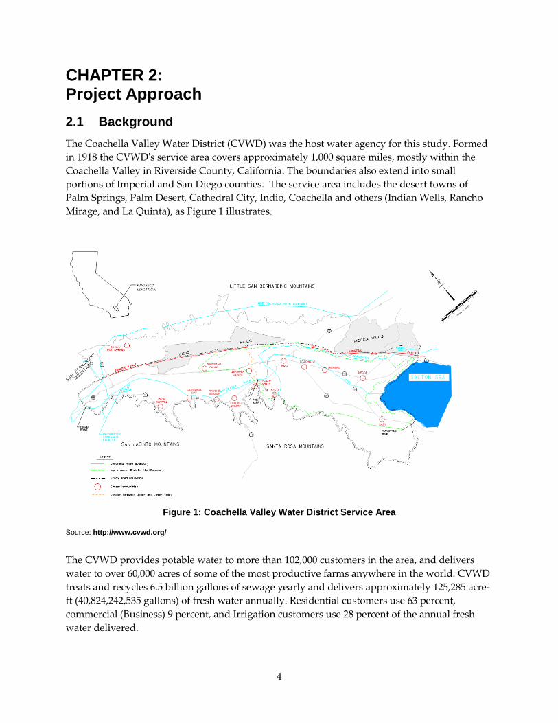
CHAPTER 2: Project Approach 2.1 Background The Coachella Valley Water District (CVWD) was the host water agency for this study. Formed in 1918 the CVWD's service area covers approximately 1,000 square miles, mostly within the Coachella Valley in Riverside County, California. The boundaries also extend into small portions of Imperial and San Diego counties. The service area includes the desert towns of Palm Springs, Palm Desert, Cathedral City, Indio, Coachella and others (Indian Wells, Rancho Mirage, and La Quinta), as Figure 1 illustrates.
Figure 1: Coachella Valley Water District Service Area
Source: http://www.cvwd.org/
The CVWD provides potable water to more than 102,000 customers in the area, and delivers water to over 60,000 acres of some of the most productive farms anywhere in the world. CVWD treats and recycles 6.5 billion gallons of sewage yearly and delivers approximately 125,285 acre-ft (40,824,242,535 gallons) of fresh water annually. Residential customers use 63 percent, commercial (Business) 9 percent, and Irrigation customers use 28 percent of the annual fresh water delivered.
4

For this study the area of the City of Palm Desert was the selected location – specifically, a one mile radius of the CVWD district office in Palm Desert, California. This area is in a single pressure zone, which made the water and energy usage determinations more straightforward. The single pressure zone enabled all data from the AMR meters to be compiled from a single fixed base system and automatically transferred to the CVWD district office.
Three customer classes represented in virtually all water districts were selected for participation in this study: Residential, commercial or Business, and Irrigation customers1. Residential users are defined as single family homes. The commercial customers selected were established shopping areas (strip malls) common to all water districts. Irrigation customers selected were composed of landscape meters, typically around commercial centers or common areas in housing developments.
Letters were sent to all applicable Residential, Business, and Irrigation customers in this area (411 Residential, 141 Business, and 47 Irrigation customers) advising them of this study and asking if they were willing to participate2. A total of 73 customers responded and said they would like to participate in the study (52 Residential, 11 Business and 10 Irrigation). The responding customers were incorporated into the study by assigning them to the Intervention group in their customer class. An equivalent number of non-respondents in these customer classes were randomly placed in the Control group.
The study was composed of two groups in each customer category: a Control group which had the AMR meters installed, and an Intervention group which had AMR meters installed and given instructions to minimize their water use during the electric utility (Southern California Edison) summer on-peak period, defined as 12 noon to 6pm weekdays from June 1 through October 2. The Intervention group was given an incentive of $25 per month (provided by the City of Palm Desert). There were a total of 147 initial participants in the study: 52 Residential Intervention and 52 Residential Control, 11 Business Intervention and 12 Business Control, and 10 Irrigation Intervention and 11 Irrigation Control customers.
2.2 Meter Requirements The Coachella Valley Water District used the following criteria to select a water meter for the Time of Use study.
Capabilities - The meter must be Multi-jet technology that meets all AWWA Standards and NSF Certified, able to withstand suspended matter, entrained solids, and high mineral contents, while providing prolonged accuracy. Meters must be connection free with no wires, tamper proof, and be capable of providing leak detection and data logging. Compatibility must be present between the meters and existing infrastructure (Green Tree Software), and must be available in various sizes ranging from ¾” to 2”, depending upon the account interconnection size.
1 This area has no industrial water customers. 2 On February 9, 2009.
5

Number of Meters – One meter was needed per participant in the study, for a total of 148 meters installed for this study. The type, meter size, and quantity are as follows:
Type Size Control Group Test Group Residential ¾ 53 53 Business 1” 14 14 Landscaping 1 ½” 7 7
Infrastructure – In addition to the actual meters themselves, boosters and antennas (repeater and concentrator) were required to transmit the interval water use data to the district office. The CVWD currently uses the Master Meter Dialog 3G Mobile AMR system for the monthly reading of 10,673 water meters system wide. A key benefit of the Dialog 3G system is its ability to easily migrate to a fixed network AMI system without losing the mobile AMR capabilities. This time of use study required hourly readings as close to the top of each hour as possible. By adding a wireless Meter Interface Unit (MIU) to existing meter installations, the Dialog 3G meter integrated radios could forward 15 minute meter reading data and alarms over the proposed fixed network AMI system. The product name for the MIU is the Dialog 3G Booster; the fixed network product name is FixedLinx (www.FixedLinx.com); both products are manufactured by Master Meter.
AMR meters for all participants and the fixed base system were installed by CVWD personnel and Master Meter Inc. in March and April 2009 (for a description of the system and its installation procedures, consult Appendix A).
An informational meeting was held at the CVWD district office on March 18, 2009, for participants in the Intervention groups. The meeting described the project and introduced them to the project web site, on which participants in the Intervention groups could get details about the project and see their water usage on 15 minute intervals. A letter detailing this information was also sent out to all the customers in the Intervention groups, along with their individualized password that allowed them to view their water use data.
May 1st was the go live date, in which all components of the project (meter readings, data transfer, web page, and statistical analyses) were activated. This allowed a full test of all components of the study prior to the actual study start date. Participants were allowed to test out peak period water use shifting strategies.
The actual study period ran from June 1 through October 2, 2009. Meter data was also collected and analyzed for the month of October to determine if the behavior patterns established during the test period carried over after the study was completed.
A final public meeting to convey the results of the study was held at the CVWD district office on March 1, 2010, for participants in the study.
2.3 Data and Statistical Analysis The AMR meters record water usage in 15 minute intervals. The 15 minute interval meter data was collected to provide hourly water usage by both Intervention and Control participants in
6

Residential, Business, and Irrigation customer classes (see Appendix B for data manipulations and summaries of statistical analyses).
Three CVWD (Coachella Valley Water District) customer groups in the City of Palm Desert are examined: single family Residential, Business (small commercial businesses in strip malls), and Irrigation (landscape) customers. In each customer class there was a Control group and an Intervention group.
Water Research Questions Addressed in This Study
1. Is the water use of customers participating in this study accurately representing the water use of the selected customer class?
To identify if customers participating in the study truly represented the populations they were selected from, total water use for the month of May, 2009, (pre-test period) was assessed. The total May water use of the study participants was compared to the May total water use of the population (May Residential study participants water use was compared to the May CVWD Residential population water use).
2. After applying an incentive to the Intervention (test) groups, will the Intervention groups reduce water use during the 12noon- 6pm weekday times? The Intervention groups received $25 per month as an incentive to reduce their water use during 12 noon- 6pm on weekdays. For each of the three customer classes, the hourly water use by the Intervention group during 12 noon- 6pm weekday was compared to the water use by the Control group. Results were compared using nonparametric analyses (see Appendix B).
3) Compared to the Control groups, will the Intervention groups use less water overall or simply shift water use out of the peak period? There is a question as to whether peak period water shifting is a conservation measure. The relationship between altered peak water use and the impact on total water use has not been previously investigated. Does a reduction in peak water use lead to changes in total water use? For each of the three groups, the total monthly water use by the Intervention group was compared to the water use by the Control group.
Embedded Energy in Water
The embedded energy in water (kWh/mgal – the amount of electricity required to treat and deliver the water) from the CVWD Valley Zone was determined, in order to develop estimates of the amount of energy (kWh) and peak demand (kW) reduced by the test groups water shifting behavior.
Monthly Average – Monthly electrical use from all electric accounts in the CVWD Valley Zone was compared with monthly CVWD water send-out data in order to determine average embedded energy (kWh per gallon).
Daily Peak - Electrical use from all electric accounts in the CVWD Valley Zone for the summer peak electrical demand day was compared with CVWD water send-out data on a 24 hour basis in order to determine average embedded energy per hour over a typical monthly day.
7

The average 12 noon-6 pm weekday water reduction was multiplied by the daily peak embedded energy in water to determine the peak energy/demand reduction.
8

CHAPTER 3: Project Results 3.1 Representativeness of Study Participants One of the concerns about any study is how transferrable are the results of the study to the general population; that is, will the results of this study be applicable to the general water customer? In order to assess this question, water use characteristics of the study participants was compared to the water use characteristics of the population. Pre-study (May) water use profiles for the participants in the study were compared to the May water use profiles for the entire CVWD customer class these participants were drawn from.
Residential: A comparison of the May water use of the Residential study participants with the total CVWD Residential population is shown in Figure 2. A total of 102 Residential customers (51 assigned to the Control group and 51 assigned to the Intervention group) participated in this study. The CVWD Residential class average for the entire CVWD Valley zone for May was 19,793 gallons, a value lower than the mean water use by the Residential participants in this study (25,600 gallons3). The median of the May Residential population water use was 9,724 gallons, while the median of the study population 21,254 gallons. In this area there are a number of vacation homes, which record very little or no water usage when unoccupied. These minimal water usage Residential customers were eliminated from the study. Based upon the distribution in Figure 2, it is also obvious that there are some Residential customers who use very large amounts of water, skewing the distribution to the right.
Discrepancies between the median values and mean values indicates that there exist, in both the population as well as in the study participants, customers that use large amounts of water. Such indications are evident by a positive skewing of the distribution; a majority of the data points from customer water use are clustered to the left-hand side of the histogram. Because of the skewness, conducting analyses that assume a normal distribution of the data may not be trustworthy, requiring the use of nonparametric methods of analysis. The Residential participants in this study use a greater amount of water than the CVWD Residential population, but their distribution is much more normally distributed than the general population4.
There was no statistically significant difference between the May water use of the Residential customers in the Intervention group and in the Control group.
3 After all zero and minimal use customers (less than 1,496 gallons (2 ccf)) were factored out. 4 The study participants mean and median water use are much closer, the standard deviation is lower, and the skewness and kurtosis indicators are smaller – see Appendix B.
9
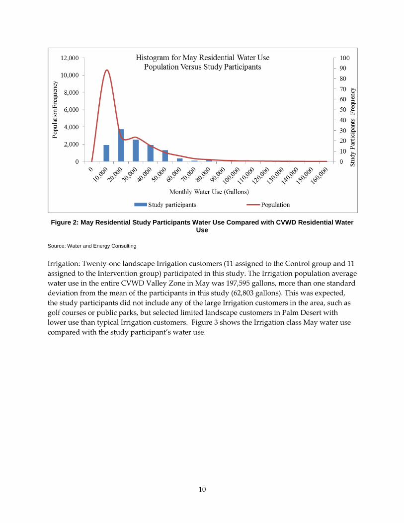
Figure 2: May Residential Study Participants Water Use Compared with CVWD Residential Water
Use
Source: Water and Energy Consulting
Irrigation: Twenty-one landscape Irrigation customers (11 assigned to the Control group and 11 assigned to the Intervention group) participated in this study. The Irrigation population average water use in the entire CVWD Valley Zone in May was 197,595 gallons, more than one standard deviation from the mean of the participants in this study (62,803 gallons). This was expected, the study participants did not include any of the large Irrigation customers in the area, such as golf courses or public parks, but selected limited landscape customers in Palm Desert with lower use than typical Irrigation customers. Figure 3 shows the Irrigation class May water use compared with the study participant’s water use.
10

Figure 3: May Irrigation Study Participants Water Use Compared with CVWD Irrigation Water Use
Source: Water and Energy Consulting
Business: Twenty-one Business customers (11 assigned to the Control group and 10 assigned to the Intervention group) participated in this study. The Business population average water use in the CVWD Valley Zone during May was 27,080 gallons during the month, comparable with the average water use of the Business participants in this study (26,640 gallons). Only strip mall customers were used for participation in this study, not the entire Business population. As the following Figure 4 shows, there are several large users in the Business study that can overwhelm the water use of the rest of the study participants.
11

Figure 4: May Business Study Participants Water Use Compared with CVWD Business Water Use
Source: Water and Energy Consulting
3.2 Leak Detection While not a central focus of this study, a benefit of AMR meters is the capability to automatically detect leaks on the customer’s premises. The smart meter manufactured by Master Meter is programmed for automatic leak detection. A leak is reported when there has been a continuous recorded flow of water for 24 hours (i.e., the meter does not register at least one zero - no water use - during at least one 15 minute interval). It will continue to show the leak report until there is a three hour period of non-flow. This leak alert can be seen instantly if the water usage information is automatically transferred to a central receiving point via a fixed base system or will be observed in the monthly reads if the meter is accessed via drive by.
When the leak alarm was received, it was noted on the website for this study and an email was sent to notify the leaking participant. Water usage was rechecked and participants were notified if the leaks are not corrected within one month. No follow-up other than notification of the leak was conducted for this study. Participants in both the Intervention and Control groups were notified of leaks.
Figure 5 shows a Residential customer with a leak of about 5 gallons per hour, while Figure 6 shows a Residential customer with no water leakage.
12

Figure 5: Residential Customer Hourly Water Use With Water Leak
Source: Water and Energy Consulting
Figure 6: Residential Customer Hourly Water Use With No Leaks
Source: Water and Energy Consulting
13

3.2.1 Residential Group During the duration of this study, approximately 30 percent of the Residential customers experienced a leak. There were 29 leaks reported out of the 102 participants in the Residential group. The leaks were evenly distributed between the Intervention group and the Control group. Participants in both the Intervention and Control groups were notified of the leaks.
Of the leaks detected, over 70 percent were temporary, such as a hose or faucet left on, which are usually remedied with ease. These types of leaks, though infrequent, have the potential to be quite large, as a hose left on can waste 250 gallons per hour.
More persistent leaks, such as a leaking toilet, faucet, or Irrigation sprinkler, required the customer to repair or replace a component of their water system. Approximately 28 percent of the Residential leaks identified required component repair or replacement. Leaking faucets can waste one gallon per hour or more, whereas leaking sprinklers can waste up to 50 gallons per hour.
Residential leaks in this study waste approximately 165,000 gallons per month, about 7 percent of the total Residential water use.
3.2.2 Irrigation Group Approximately 15 percent of the Irrigation group experienced leaks during this study. Most of the leakage in this group was due to some functional component failure, generally a fault in an Irrigation timer. Irrigation leaks wasted about 45,000 gallons per month, or about 3 percent of the total Irrigation water use.
3.2.3 Business Group The Business group had approximately 30 percent experiencing leaks during this study. These leaks were generally due to some functional component failure, such as a running urinal or toilet). Business leaks used about 36,000 gallons per month, or about 6 percent of the total Business use.
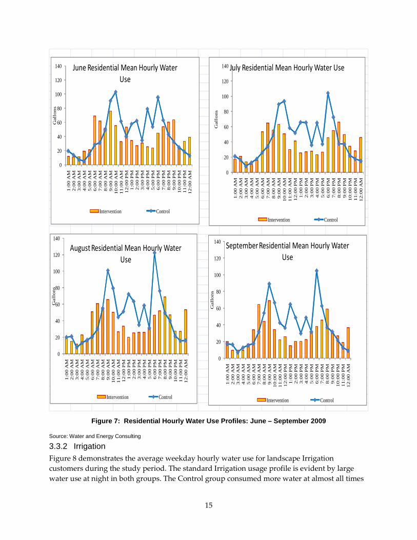
3.3 Water Usage - Hourly 3.3.1 Residential Figure 7 shows the hourly Residential weekday water use patterns during the course of this study. The Residential Intervention group (orange bars) demonstrated a significant shift of water use out of the peak period, reducing peak period water use compared to the Control group (blue line), and increased their off peak water use compared to the Control group consistently throughout the study.
14
0
20
40
60
80
100
120
1401:
00 A
M2:
00 A
M3:
00 A
M4:
00 A
M5:
00 A
M6:
00 A
M7:
00 A
M8:
00 A
M9:
00 A
M10
:00
AM
11:0
0 A
M12
:00
PM
1:00
PM
2:00
PM
3:00
PM
4:00
PM
5:00
PM
6:00
PM
7:00
PM
8:00
PM
9:00
PM
10:0
0 P
M11
:00
PM
12:0
0 A
M
Gal
lons
June Residential Mean Hourly Water Use
Intervention Control
0
20
40
60
80
100
120
140
1:00
AM
2:00
AM
3:00
AM
4:00
AM
5:00
AM
6:00
AM
7:00
AM
8:00
AM
9:00
AM
10:0
0 A
M11
:00
AM
12:0
0 P
M1:
00 P
M2:
00 P
M3:
00 P
M4:
00 P
M5:
00 P
M6:
00 P
M7:
00 P
M8:
00 P
M9:
00 P
M10
:00
PM
11:0
0 P
M12
:00
AM
Gal
lons
July Residential Mean Hourly Water Use
Intervention Control
0
20
40
60
80
100
120
140
1:00
AM
2:00
AM
3:00
AM
4:00
AM
5:00
AM
6:00
AM
7:00
AM
8:00
AM
9:00
AM
10:0
0 A
M11
:00
AM
12:0
0 P
M1:
00 P
M2:
00 P
M3:
00 P
M4:
00 P
M5:
00 P
M6:
00 P
M7:
00 P
M8:
00 P
M9:
00 P
M10
:00
PM
11:0
0 P
M12
:00
AM
Gal
lons
September Residential Mean Hourly Water Use
Intervention Control
0
20
40
60
80
100
120
140
1:00
AM
2:00
AM
3:00
AM
4:00
AM
5:00
AM
6:00
AM
7:00
AM
8:00
AM
9:00
AM
10:0
0 A
M11
:00
AM
12:0
0 P
M1:
00 P
M2:
00 P
M3:
00 P
M4:
00 P
M5:
00 P
M6:
00 P
M7:
00 P
M8:
00 P
M9:
00 P
M10
:00
PM
11:0
0 P
M12
:00
AM
Gal
lons
August Residential Mean Hourly Water Use
Intervention Control
Figure 7: Residential Hourly Water Use Profiles: June – September 2009
Source: Water and Energy Consulting
3.3.2 Irrigation Figure 8 demonstrates the average weekday hourly water use for landscape Irrigation customers during the study period. The standard Irrigation usage profile is evident by large water use at night in both groups. The Control group consumed more water at almost all times
15

compared to the Intervention group. There is no clear pattern of the Irrigation customers shifting water use out of the peak period.
16

0
100
200
300
400
500
600
700
1:0
0 A
M
3:0
0 A
M
5:0
0 A
M
7:0
0 A
M
9:0
0 A
M
11
:00
AM
1:0
0 P
M
3:0
0 P
M
5:0
0 P
M
7:0
0 P
M
9:0
0 P
M
11
:00
PM
Ga
llo
ns
August Irrigation Mean Hourly Water Use
Intervention Control
0
100
200
300
400
500
600
700
1:0
0 A
M2
:00
AM
3:0
0 A
M4
:00
AM
5:0
0 A
M6
:00
AM
7:0
0 A
M8
:00
AM
9:0
0 A
M1
0:0
0 A
M1
1:0
0 A
M1
2:0
0 P
M1
:00
PM
2:0
0 P
M3
:00
PM
4:0
0 P
M5
:00
PM
6:0
0 P
M7
:00
PM
8:0
0 P
M9
:00
PM
10
:00
PM
11
:00
PM
12
:00
AM
Ga
llo
ns
September Irrigation Mean Hourly Water Use
Intervention Control
0
100
200
300
400
500
600
7001
:00
AM
2:0
0 A
M3
:00
AM
4:0
0 A
M5
:00
AM
6:0
0 A
M7
:00
AM
8:0
0 A
M9
:00
AM
10
:00
AM
11
:00
AM
12
:00
PM
1:0
0 P
M2
:00
PM
3:0
0 P
M4
:00
PM
5:0
0 P
M6
:00
PM
7:0
0 P
M8
:00
PM
9:0
0 P
M1
0:0
0 P
M1
1:0
0 P
M1
2:0
0 A
M
Ga
llo
ns
June Irrigation Mean Hourly Water Use
Intervention Control
0
100
200
300
400
500
600
700
1:0
0 A
M2
:00
AM
3:0
0 A
M4
:00
AM
5:0
0 A
M6
:00
AM
7:0
0 A
M8
:00
AM
9:0
0 A
M1
0:0
0 A
M1
1:0
0 A
M1
2:0
0 P
M1
:00
PM
2:0
0 P
M3
:00
PM
4:0
0 P
M5
:00
PM
6:0
0 P
M7
:00
PM
8:0
0 P
M9
:00
PM
10
:00
PM
11
:00
PM
12
:00
AM
Ga
llo
ns
July Irrigation Mean Hourly Water Use
Intervention Control
Figure 8: Irrigation Hourly Water Use Profiles: June – September 2009
Source: Water and Energy Consulting
17

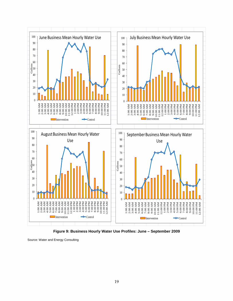
3.3.3 Business Figure 9 shows the average weekday water use for Business participants during the study period. As the graph shows, several large Business participants in the Intervention group used significant amounts of water starting at 4 am, 6 pm, and 11 pm weekdays every month (likely food preparation businesses or bakeries). Once those customers were factored out, both the Intervention and Control groups demonstrated qualitatively similar water use, using water predominantly during 8am-5pm, considered normal business hours.
18
0
10
20
30
40
50
60
70
80
90
1001:
00 A
M2:
00 A
M3:
00 A
M4:
00 A
M5:
00 A
M6:
00 A
M7:
00 A
M8:
00 A
M9:
00 A
M10
:00
AM
11:0
0 A
M12
:00
PM
1:00
PM
2:00
PM
3:00
PM
4:00
PM
5:00
PM
6:00
PM
7:00
PM
8:00
PM
9:00
PM
10:0
0 P
M11
:00
PM
12:0
0 A
M
Gal
lons
June Business Mean Hourly Water Use
Intervention Control
0
10
20
30
40
50
60
70
80
90
100
1:00
AM
2:00
AM
3:00
AM
4:00
AM
5:00
AM
6:00
AM
7:00
AM
8:00
AM
9:00
AM
10:0
0 A
M11
:00
AM
12:0
0 P
M1:
00 P
M2:
00 P
M3:
00 P
M4:
00 P
M5:
00 P
M6:
00 P
M7:
00 P
M8:
00 P
M9:
00 P
M10
:00
PM
11:0
0 P
M12
:00
AM
Gal
lons
July Business Mean Hourly Water Use
Intervention Control
0
10
20
30
40
50
60
70
80
90
100
1:00
AM
2:00
AM
3:00
AM
4:00
AM
5:00
AM
6:00
AM
7:00
AM
8:00
AM
9:00
AM
10:0
0 A
M11
:00
AM
12:0
0 P
M1:
00 P
M2:
00 P
M3:
00 P
M4:
00 P
M5:
00 P
M6:
00 P
M7:
00 P
M8:
00 P
M9:
00 P
M10
:00
PM
11:0
0 P
M12
:00
AM
Gal
lons
September Business Mean Hourly Water Use
Intervention Control
0
10
20
30
40
50
60
70
80
90
100
1:00
AM
2:00
AM
3:00
AM
4:00
AM
5:00
AM
6:00
AM
7:00
AM
8:00
AM
9:00
AM
10:0
0 A
M11
:00
AM
12:0
0 P
M1:
00 P
M2:
00 P
M3:
00 P
M4:
00 P
M5:
00 P
M6:
00 P
M7:
00 P
M8:
00 P
M9:
00 P
M10
:00
PM
11:0
0 P
M12
:00
AM
Gal
lons
August Business Mean Hourly Water Use
Intervention Control
Figure 9: Business Hourly Water Use Profiles: June – September 2009
Source: Water and Energy Consulting
19

3.4 Peak Period Water Use An indication of whether customers shifted water use out of the peak period can be determined using a peak percentage5. The peak percentage is a formula that calculates the ratio of weekday peak water use to the weekday total water use. If a customer was to hypothetically consume water continuously over a 24 hour period, the peak percentage would be 25 percent6. A peak percentage greater than 25 percent indicates that the customer is using more water during the peak period, where a peak percentage less than 25 percent indicates that the customer is using more water during the non-peak hours.
3.4.1 Residential An indication of the Residential water use can be found in the Table 1. It shows the percentage of the total water use during weekdays that occurred in the peak period. The Intervention group is clearly shifting a significant amount of their peak period water use out of the peak period to the other hours of the day.
Table 1: Residential Peak Percentage Water Use
Residential Peak as %
of Total Water Use
Control Intervention
June 36.70% 19.88%
July 30.91% 20.33%
August 36.06% 19.83%
September 36.05% 20.35%
Ave 34.93% 20.10%
Figure 10 illustrates the difference in peak water usage between the Residential Intervention and Residential Control groups. The Residential Intervention participants used less than one-half the amount of water compared to the Control group during the peak period, with each Residential customer saving an average of over 4,000 gallons of peak water use during the month.
5 Peak Percentage is defined as the amount of water consumed during the six hour on-peak period divided by the total daily water consumption. 6 6 hours / 24 hours = 25%.
20

Figure 10: Residential Peak Period Water Use: Intervention and Control Group
Source: Water and Energy Consulting
3.4.2 Irrigation The Irrigation customer peak percentage water use for both Intervention and Control groups is found in Table 2. Compared to the Business and Residential groups, the low values support the notion that Irrigation customers prefer to use water at night, thereby lowering their water use during daylight hours, including peak hours. The Intervention groups used a greater amount of their total water use during the peak periods compared to the Control group.
Table 2: Irrigation Peak Percentage Water Use
Irrigation Peak as % of Total Water UseControl Intervention
June 12.12% 16.25%July 6.73% 17.10%August 7.69% 16.33%September 12.08% 16.80%
ave 9.65% 16.62% Source: Water and Energy Consulting
21
3.4.3 Business The Business customer peak percentage water use can be found in Table 3. Businesses are open during standard business hours, so one would expect them to be using more water during the daytime when the business is open, indicated by peak percentages greater than 25 percent. Interestingly, the Business Intervention group shifted almost one-quarter (based on the averages listed) of peak period water use to the non-peak business hours.
Table 3: Business Peak Percentage Water Use
Business Peak as % of Total Water UseControl Intervention
June 40.91% 35.39%July 42.94% 17.10%August 43.79% 34.44%September 39.77% 35.54%
ave 41.85% 30.62% Source: Water and Energy Consulting
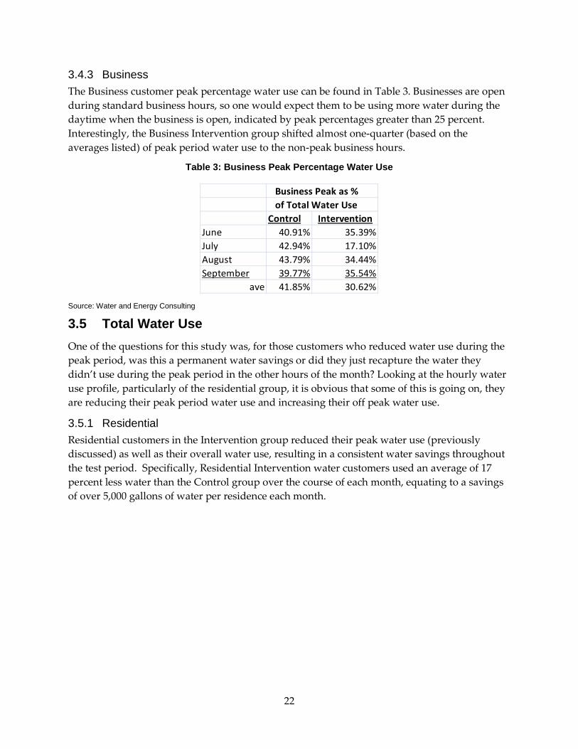
3.5 Total Water Use One of the questions for this study was, for those customers who reduced water use during the peak period, was this a permanent water savings or did they just recapture the water they didn’t use during the peak period in the other hours of the month? Looking at the hourly water use profile, particularly of the residential group, it is obvious that some of this is going on, they are reducing their peak period water use and increasing their off peak water use.
3.5.1 Residential Residential customers in the Intervention group reduced their peak water use (previously discussed) as well as their overall water use, resulting in a consistent water savings throughout the test period. Specifically, Residential Intervention water customers used an average of 17 percent less water than the Control group over the course of each month, equating to a savings of over 5,000 gallons of water per residence each month.
22
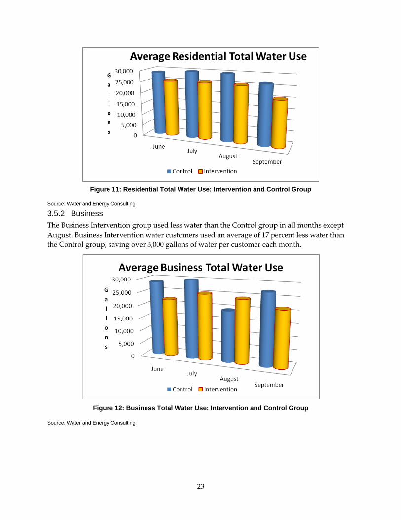
Figure 11: Residential Total Water Use: Intervention and Control Group
Source: Water and Energy Consulting
3.5.2 Business The Business Intervention group used less water than the Control group in all months except August. Business Intervention water customers used an average of 17 percent less water than the Control group, saving over 3,000 gallons of water per customer each month.
Figure 12: Business Total Water Use: Intervention and Control Group
Source: Water and Energy Consulting
23

3.6 Statistical Significance For a detailed description of data analyses and summary statistics reported in this study, see Appendix B. Due to the skewed (non-normal) distribution of the data in the samples (see section 3.1–3.3), the use of parametric analyses may be inappropriate to summarize the data7. In order to evaluate the water use profiles of the various customer classes, a Mann-Whitney U test was utilized. This nonparametric method of analysis allowed the statistical comparison of water use profiles between the Intervention group and the Control group for all combinations of customer classes (Residential, Irrigation, and Business) and months of study duration (the months of June, July, August, and September).
A summary of the statistical results for the duration of the study are provided in the following Table 4. The Residential Intervention peak water use is significantly less than the Control during all months of the study (alpha level of 0.05); with the overall water use in the Residential Intervention group being significantly lower that the Control group in September, the last month of the study. Changes in peak and overall water use patterns were not statistically significant in the other customer groups.
Table 4: Study Statistical Summary
Control Mean
(Average) gallons
Intervention Mean
(Average) gallons
Control Median gallons
Intervention Median gallons
Median Significance
June Residential Monthly 28,933 25,282 26,483 24,460 0.322
Business Monthly 28,652 22,179 7,405 17,189 0.498
Irrigation Monthly 104,607 68,055 29,378 47,524 0.510
Residential Peak* 7,558 3,055 5,509 1,765 0.000
Business Peak 10,124 6,461 3,998 5,430 0.667
Irrigation Peak 8,944 6,606 277 5,819 0.203
Residential Non-
Peak 23,779 22,174 20,159 21,939 0.812
Business Non-Peak 20,915 14,457 3,867 12,492 0.538
Irrigation Non-Peak 95,550 53,247 29,071 35,724 1.000
7 Three groups are necessary for a parametric analysis: 1) Normality of the dependent variable distribution: The data should be approximately normally distributed (a bell shaped curve), 2) Homogeneity of variance: called homoscedasticity, defined as the variance of data in groups should be the same, 3) Independent observations: results for one group should not be dependent on another variable or group.
24

July Residential Monthly 31,180 25,541 28,005 23,719 0.108
Business Monthly 30,871 25,248 7,547 17,069 0.498
Irrigation Monthly 128,038 62,907 56,429 44,450 0.360
Residential Peak* 7,757 3,489 5,258 2,072 0.000
Business Peak 9,971 6,831 4,121 5,685 0.712
Irrigation Peak 7,242 8,381 583 7,218 0.056
Residential Non-
Peak 30,145 26,336 26,528 23,351 0.174
Business Non-Peak 20,899 18,416 3,830 10,756 0.325
Irrigation Non-Peak 120,796 54,526 55,423 33,391 0.391
August Residential Monthly 30,462 25,464 30,859 21,976 0.064
Business Monthly 19,606 24,268 7,102 14,967 0.196
Irrigation Monthly 123,919 64,318 58,120 48,003 0.429
Residential Peak* 7,228 3,229 6,452 1,578 0.000
Business Peak 8,349 7,072 3,467 5,229 0.580
Irrigation Peak 6,533 7,635 628 7,955 0.145
Residential Non-
Peak 23,448 21,136 21,019 18,693 0.251
Business Non-Peak 14,999 17,196 5,199 9,739 0.325
Irrigation Non-Peak 117,405 56,684 56,059 36,331 0.291
September Residential Monthly* 26,687 20,628 24,875 17,877 0.022
Business Monthly 27,357 21,591 7,873 15,312 0.498
Irrigation Monthly 97,188 59,473 66,220 37,968 0.166
Residential Peak* 6,408 2,809 4,817 1,750 0.000
Business Peak 8,006 6,272 2,588 5,199 0.356
Irrigation Peak 7,655 6,734 1,496 6,781 0.305
Residential Non-
Peak 21,229 17,819 18,319 14,766 0.172
Business Non-Peak 19,351 15,319 4,095 10,113 0.295
25
Irrigation Non-Peak 89,534 52,740 55,823 28,959 0.147
* = significant at the 0.05 level Source: Water and Energy Consulting
3.7 Behavior Persistence Though not a central focus of this study, water use data was collected through October to identify if water consumption behavior observed during the study period would continue or persist after the study ended. Based on the outcomes below, it is apparent that the reductions in peak water use for all groups continued after the study was completed; a very encouraging result, suggesting that an Intervention such as this one has the potential to beneficially alter the water use profiles of customers.
3.7.1 Peak Water Use Reduction - October Residential
Residential customers in the Intervention group used 60 percent less peak water than the Control group during June, 55 percent less than the Control group in July, 45 percent less than the Control group in August, and 56 percent less than the Control group in September. During the month of October (after the study was officially completed), the Residential Intervention group continued to use significantly less (32 percent less) water during peak hours compared to their Control group counterparts. Though less than the reduction during the study, the October reduction indicates that Residential behavior persists after the incentive has been removed and the participants are aware that they are not encouraged to use less water.
Irrigation
The Irrigation Intervention customers using 26 percent less peak water than their Control counterparts for the month of June, a greater amount of peak water than the Control group in July and August, and 12 percent less during the month of September. During October, the Irrigation Intervention customers demonstrated 11 percent less peak water use than the Control group.
Business
The month of June saw the Business Intervention group use 26 percent less peak water than their Control counterparts, 32 percent less than the Control group during July, 15 percent less than the Control group during August, and 22 percent less peak water than the Control group during the month of September. During the month of October, Business customers in the Intervention group used 43 percent less peak water than the Control group.
3.8 Embedded Energy Energy is used in all stages of the water use cycle (Figure 13). Water is diverted, collected, or extracted from a source. It is transported to water treatment facilities, treated, and then distributed to end users. Wastewater from urban uses is collected, treated, and discharged back to the environment, or is recycled to become a water source for someone else. The embedded
26

energy in water is simply how much energy is necessary to provide water at various stages of the water use cycle8. Determining the amount of energy that is necessary to provide water is a useful tool in evaluating how much energy can be saved when water is conserved or evaluating how much energy will be necessary when a new source of water is used9.
Figure 13: California Water Use Cycle Embedded Energy
Source: 2005 Integrated Energy Report10
The domestic water system serving the Palm Desert area of the Coachella Valley Water District is a fairly typical domestic water system. The water supply is groundwater, pumped from wells distributed throughout the area (Figure 14). The distribution system generally consists of a grid-like layout of piping, with 18” and 24” pipelines along section line roadways forming the
8 California Energy Commission, “California’s Water-Energy Relationship”, CEC-700-2005-011-SF, November 2005.
9 California Energy Commission, “Refining Estimated Of Water-Related Energy Use in California”, CEC-500-2006-118, December 2006.
10 California Energy Commission, “Integrated Energy Policy Report”, CEC-100-2005-007CMF, November 2005, Chapter 6: Integrating Water and Energy Strategies.
27

backbone of the system. Smaller pipelines distribute the water to businesses and neighborhoods, with some customers served directly from the larger backbone pipelines. Wells pump directly into the pipeline grid. The water flows under pressure through the system to customers and to steel tank storage reservoirs. There are booster pumps where necessary to pump water to higher elevation customers and to the storage. There is sufficient elevated storage to provide for fire flow. The wells are controlled using a Supervisory Control And Data Acquisition (SCADA) system that calls for wells to turn on when levels in the storage reservoirs reach pre-determined levels.
Table 5 shows the Palm Desert embedded energy calculation. The electricity use by all of CVWD’s electric accounts in the Palm Desert system (groundwater extraction wells, water treatment, distribution system pumps, and wastewater collection and treatment facilities) for the months of June, July, August, and September 2009, as well as for the electric utility peak demand day (September 3, 2009), was divided by the amount of water CVWD delivered in the Palm Desert area during these time periods. The mean CVWD embedded energy in water for this area is 4,099 kWh/mgal (1,336 kWh/af).
Table 5: CVWD Embedded Energy in Water During Summer of 2009
Water Electricity
(gallons) (kWh) kWh/gal kWh/mgal kWh/af
June 1,465,401,380 5,967,130 0.004072011 4,072 1,327
July 1,594,392,130 5,732,007 0.003595105 3,595 1,171
August 1,490,324,745 5,952,409 0.003994035 3,994 1,301
September 1,120,324,640 5,589,592 0.004989261 4,989 1,626
Peak day: 48,336,680 175,713 0.003635179 3,635 1,185
3-Sep
28

Figure 14: Palm Desert Domestic Water System
Source: Water and Energy Consulting
29
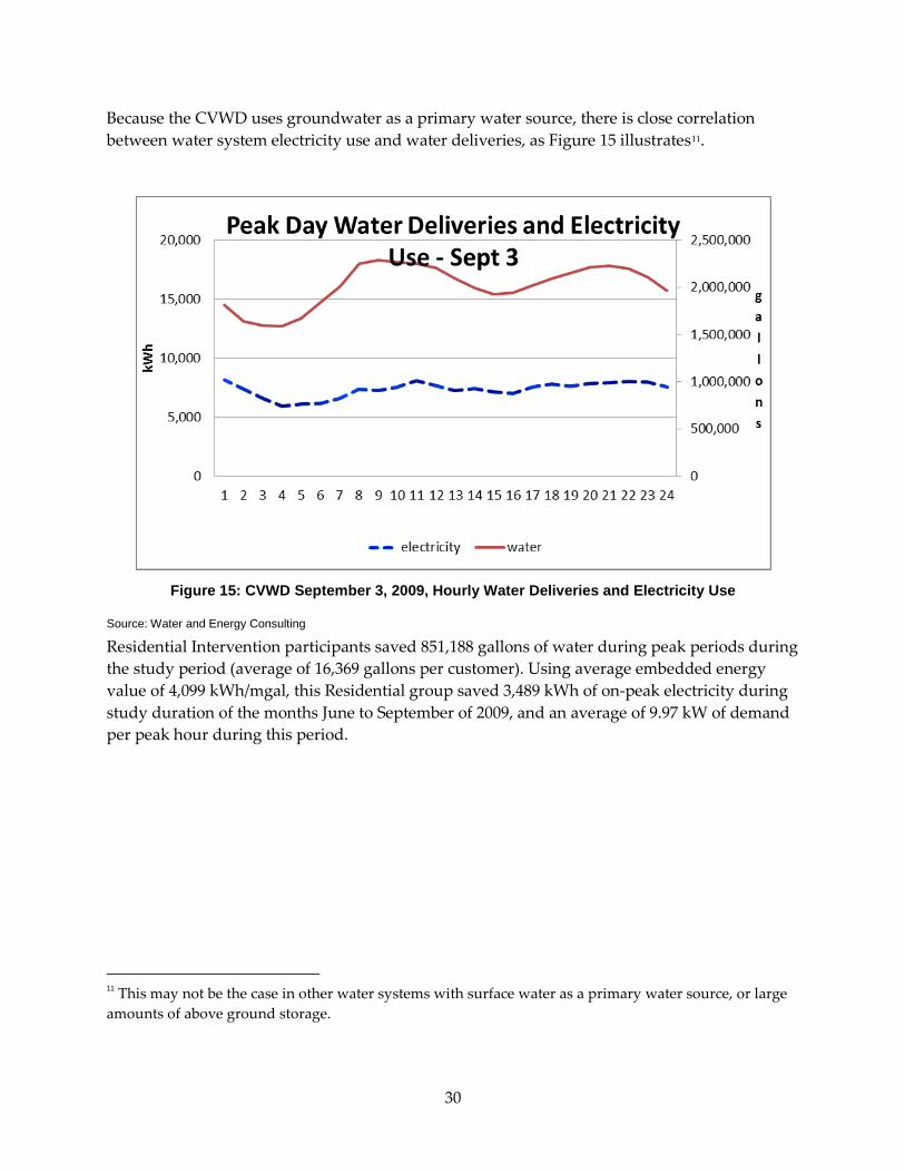
Because the CVWD uses groundwater as a primary water source, there is close correlation between water system electricity use and water deliveries, as Figure 15 illustrates11.
Figure 15: CVWD September 3, 2009, Hourly Water Deliveries and Electricity Use
Source: Water and Energy Consulting
Residential Intervention participants saved 851,188 gallons of water during peak periods during the study period (average of 16,369 gallons per customer). Using average embedded energy value of 4,099 kWh/mgal, this Residential group saved 3,489 kWh of on-peak electricity during study duration of the months June to September of 2009, and an average of 9.97 kW of demand per peak hour during this period.
11 This may not be the case in other water systems with surface water as a primary water source, or large amounts of above ground storage.
30

CHAPTER 4: Conclusions and Recommendations 4.1 Leaks The AMR meter leak detection identified leaks totaling almost 250,000 gallons per month, or over 5 percent of the total water use by all participants (in both Intervention and Control groups) in this study.
Though the use of smart (AMR) meters in identifying leakage is well established12, comparing the results of this study with other leakage studies is difficult due to discrepancies in the definition of leakage. As previously noted, in this study any 24 hour continuous water usage was flagged as a leak. A majority of leaks were of limited duration; for instance, a faucet or hose left running. In most other water leakage studies, leaks are defined as a continuous water loss (generally multi-day) that is the result of some component failure, with corrective action (replacement or repair) being necessary to fix the leak. Leaks can be the largest single component of Residential indoor water use13, but typically a small number of homes are responsible for most of the leakage according to a 1999 American Water Works Association study called “Residential End Uses of Water”. The number of persistent Residential leaks in this study (10 percent of participants) falls within the range of Residential leakage found elsewhere. For example, a study in Northern California found between 10 and 40 percent of Residential customers recorded leaks14.
In this study, study participants (both Intervention and Control) were merely informed of detected leaks. While they were not required to fix them, the vast majority of those notified addressed the issue. However, some customers who failed to remedy the situation despite numerous notifications. Figure 16 shows the water usage for one of the study participants (an Irrigation customer) during the last full week of the study. Despite numerous notices throughout the study period, this customer continued to have a leak of approximately 50 gallons per hour, similar to the leak level identified for this customer during the first week of the study. This is not an unusual occurrence; other studies have found that approximately 20 percent of leakers did not respond to any form of communication15.
12 C. Dobbie and S. Durham, 2003, “Automated Meter Reading System Helps Track Water Usage”, Waterworld, September 2003 Editorial. 13 P. Mayer, W. DeOreo, E. Towler, and D. Lewis, 2003, “Residential Indoor Water Conservation Study”, Report prepared for East Bay Municipal Utility District and the United States Environmental Protection Agency, July 2003. 14 A. Chastain-Howley and D. Wallenstein, 2007, “Using an AMR System to Aid in the Evaluation of Water Losses: A Small DMA Case Study at East Bay Municipal Utility District, USA”, Water Loss 2007 Proceedings, pg. 394-403. 15 T. Britton, G. Cole, R Stewart, and D. Wiskar, 2008, “Remote Diagnosis of Leakage in Residential Household” Australian Water Association, Water Journal, September 2008, pg 56-60.
31
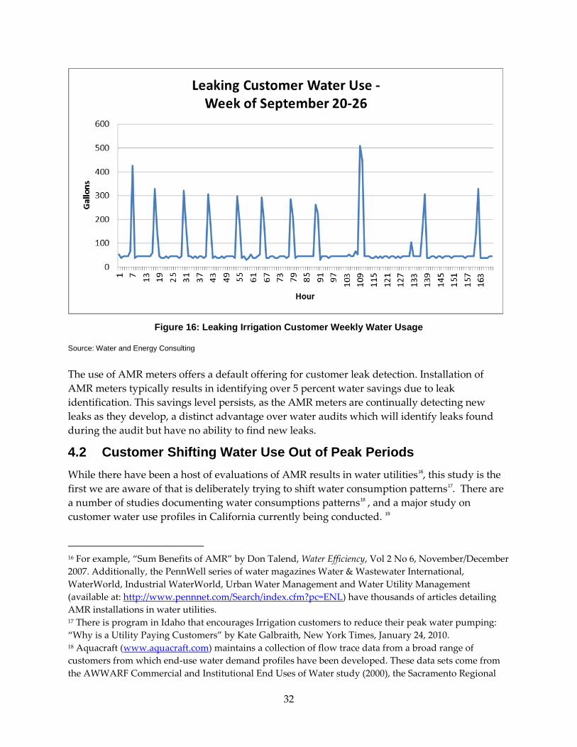
Figure 16: Leaking Irrigation Customer Weekly Water Usage
Source: Water and Energy Consulting
The use of AMR meters offers a default offering for customer leak detection. Installation of AMR meters typically results in identifying over 5 percent water savings due to leak identification. This savings level persists, as the AMR meters are continually detecting new leaks as they develop, a distinct advantage over water audits which will identify leaks found during the audit but have no ability to find new leaks.
4.2 Customer Shifting Water Use Out of Peak Periods While there have been a host of evaluations of AMR results in water utilities16, this study is the first we are aware of that is deliberately trying to shift water consumption patterns17. There are a number of studies documenting water consumptions patterns18 , and a major study on customer water use profiles in California currently being conducted. 19
16 For example, “Sum Benefits of AMR” by Don Talend, Water Efficiency, Vol 2 No 6, November/December 2007. Additionally, the PennWell series of water magazines Water & Wastewater International, WaterWorld, Industrial WaterWorld, Urban Water Management and Water Utility Management (available at: http://www.pennnet.com/Search/index.cfm?pc=ENL) have thousands of articles detailing AMR installations in water utilities. 17 There is program in Idaho that encourages Irrigation customers to reduce their peak water pumping: “Why is a Utility Paying Customers” by Kate Galbraith, New York Times, January 24, 2010. 18 Aquacraft (www.aquacraft.com) maintains a collection of flow trace data from a broad range of customers from which end-use water demand profiles have been developed. These data sets come from the AWWARF Commercial and Institutional End Uses of Water study (2000), the Sacramento Regional
32

Changing customer behavior and usage patterns (called demand response) is a well-established phenomenon for electric utilities, but is virtually unknown in the water industry. This study asked a fundamental question – is demand response from water customers on their water usage patterns a viable program for reducing water systems on-peak electrical demand?
4.2.1 Irrigation Urban Irrigation customers (landscape Irrigation) do not appear to be good candidates for reducing on-peak water use. In urban areas, these customers are typically already watering primarily at night. Golf courses and parks do not water during the day, because people are using the area during that time. Other urban landscape watering, such as landscaping around commercial buildings, also typically occurs at night, so as not to inconvenience customers and to reduce water spotting on vehicles parked in the parking lots. This study confirmed that pattern, as Table 3 shows, both the Control and Intervention groups used water predominantly during the off peak periods.
4.2.2 Commercial/Business Customers Most commercial and Business customers are open during regular Business hours, and must consume water during this period20. In this study, the customer class consisted of strip malls, using a significant amount of their water during the weekday 12noon to 6pm period (Table 4).
Water Authority CI Water Audits study (2005), the CALFED Supermarket Studies (2003) and the Monterey Pre-Rinse Spray Valve study (2003).The flow trace been used in a number of Residential, commercial, industrial and institutional water use studies both in the U.S. and worldwide including: •Heatherwood Residential End-use and Retrofit Studies – 1995-96, Aquacraft •Westminster Water Use Study – 1998, Aquacraft •Perth Residential End Uses of Water Study – 1999, Australia •Residential End Uses of Water – 1999, AWWA •Commercial and Institutional End Uses of Water – 2000, AWWA •Pinellas County Utilities Water Conservation Opportunities Study – 2002, Aquacraft •Seattle Market Penetration Study – 2003, Aquacraft •Yarra Valley Water District Residential End-use Study – 2003, Australia •EPA Residential Retrofit Studies (Seattle, EBMUD, Tampa) – 2004, Aquacraft •Water Efficiency Opportunities in California Supermarkets – 2004, Aquacraft •Monterey Pre-Rinse Spray Valve Study – 2005, Quantec •Regional Water Authority of Sacramento CII Studies – 2005, Aquacraft •Santa Paula Residential End-use Study – 2006, RBF Consulting •New Zealand Residential Demand Study – 2007, Branz •Lathrop and American Canyon, CA End-use Studies – 2008, RBF Consulting •California (CALFED) Residential End-use Baseline Study – 2009, Aquacraft •Gold Coast Water Residential End-use Study – 2009, Australia 19 Aquacraft Inc. (2009). "Embedded Energy in Water Study 3: End-use Water Demand Profile (Final Research Plan).". Available at http://uc-ciee.org/pubs/ref_water.html. 20 DeOreo, William; Peter Mayer; Benedykt Dziegielewski; Jack C Kiefer; Eva M. Opitz; Gregory A.; Porter; Glen L. Lantz and John Olaf Nelson. 2000. Commercial and Institutional End Uses of Water. Project #241B. Denver, CO: American Water Works Association Research Foundation, and Water Efficiency Manual Water for Commercial, Industrial and Institutional Facilities, a joint publication of the
33

Interestingly, the Business Intervention group did use less water during the peak period than the Control group (see Table 3 and Figure 12). The difference was not statistically significant, and it is hypothesized that it was primarily the result of outliers; several large Businesses that used large amount of water during the off peak periods (Figure 8). These Businesses may have been food preparation Business (such as bakeries and donut shops) that produced the majority of their product during the evening and early morning hours.
Further investigation should be performed to identify the potential of the Business customer class for shifting water use out of the peak period. A larger sample size may prove to be beneficial in this identification, as well as segregation of Business class by functional use (such as removing overnight food preparation customers).
4.2.3 Residential Customers One of the best examples of documented hourly Residential water use patterns is a 1999 study that was sponsored by the American Water Works Association Research Foundation (AWWARF) that quantified Residential water usage in 12 cities within the United States, of which four are located in California. Although these researchers found that there is some volumetric diversity of water use over the 12 locations, a striking conclusion of this study was that there are distinct similarities between the 12 locations in the amount of water fixtures and hourly pattern of daily water usage. The draw patterns were estimated from a Residential water use database containing nearly one million individual water use “events” collected using real-time data loggers in 1,188 residences in the 12 study sites; extensive household level information obtained through surveying of approximately 6,000 households; and historic water billing records from 12,000 residences. The study estimated hourly patterns for indoor, outdoor and total water usage. The derived time pattern of overall residential water use followed a classic diurnal pattern, as shown in Figure 17 below21:
Division of Pollution Prevention and Environmental Assistance and Division of Water Resources of the N.C. Department of Environment and Natural Resources, and Land-of-Sky Regional Council., May 2009, available at www.p2pays.org/ref/01/00692.pdf 21 DeOreo, William; Peter Mayer; Benedykt Dziegielewski; Jack C. Kiefer; Eva M. Opitz; William Davis; and John Olaf Nelson. 1999. Residential End Uses of Water. Denver, CO: American Water Works Association Research Foundation.
34

Figure 17: Typical Residential Daily Water Use Profile
Source: DeOreo et al., Residential End Uses of Water, AWWARF, 1999
The diurnal water usage pattern depicts four distinct typical characteristics, which include
- Lowest usage during the night (11 p.m. to 5 a.m.)
- Highest usage in the morning (5 a.m. to 11 a.m.)
- Moderate usage during midday (11 a.m. to 6 p.m.)
- High evening usage (6 p.m. to 11 p.m.)
This distinctive bimodal Residential water use pattern is clearly evident in the Residential water use patterns found in this study (Figure 7), and it been verified in other studies in other countries22.
Residential customer’s response in this project was surprising. The magnitude of the Residential Intervention group’s on-peak water reduction, reducing on-peak water consumption by over 50 percent (Figure 10 and Table 4), was much more impressive than anticipated. This is particularly impressive given the relatively modest incentive ($25 per month) for participating in the study and the fact there were really no disincentives for not conserving water during the peak electricity demand period.
22 For example, Heinrich, Matthias. 2007. ‘Water End Use and Efficiency Project (WEEP) – Final Report’. BRANZ Study Report 159. BRANZ Ltd, Judgeford, New Zealand; Loh, Michael, and Peter Coghlan, Domestic Water Use Study In Perth, Western Australia, Water Corporation, March 2003.
35

These results have important policy implications for California. The greatest potential for water customer demand response appears to be concentrated in the residential sector, which coincidently uses the majority of water supplied to urban areas. In California, residential customers use about 65 percent of the fresh water supplied urban areas23. For the CVWD system residential customers use almost two-thirds of all the fresh water provided. A system wide program of information and incentives to the residential sector to encourage them to reduce their on-peak water consumption may result in significant reduction in water systems on-peak water deliveries.
4.3 Peak Water Reductions as a Conservation Measure There have been limited studies on the use of smart water meters as a water conservation tool24, but the potential has been clearly identified25. With the installation of ever greater numbers of smart meters in California we would expect to see many additional uses of this technology in water conservation efforts in the next few years26.
This project was focused on shifting water use out of the peak period, and this focus, at least in the Residential sector, resulted in water conservation – the Residential customers that shifted their water use out of the on-peak period never ended up recapturing all that water. Water reductions during peak hours resulted in a 17 percent average reduction in total water used by the Residential Intervention group27.
While it would take an end-use flow trace analysis to identify exactly what water use is being curtailed during the on-peak period, we strongly suspect it is outdoor watering. As Figure 16 shows, residences typically do have outdoor water use during the hottest part of the day, the noon to 6 p.m. window. Shifting landscaping water use out of the noon to 6 pm period will result in less evapotranspiration, which would mean less water was necessary to be used to satisfy the water requirements of the landscaping.
While we would expect the potential impact of Residential shifting water use out of the 12noon to 6pm period to be large, the magnitude of the results found in this study may not be
23 California Department of Water Resources, State Water Plan, Bulletin 160 Update, Update 2005, Vol. 3, Table 1-6, pg.1-2. Available online: http://www.waterplan.water.ca.gov/cwpu2005/index.cfm. 24 Wallenstein, David Advanced Metering Systems as a Water Conservation Tool, December 13, 2007. available at http://www.cuwcc.com/WorkArea/downloadasset.aspx?id=8766 and House, Lon W. “Automatic Meter Reading (AMR)/Advancing Metering Infrastructure (AMI) Opportunities in Water” Sigma XI Year of Water White Papers, available at: http://www.sigmaxi.org/programs/issues/whitepapers.shtml, October 2008.
25 “Automatic Meter Reading (AMR)/Advancing Metering Infrastructure (AMI) Opportunities in Water” Sigma XI Year of Water White Papers, available at: http://www.sigmaxi.org/programs/issues/whitepapers.shtml, October 2008. 26 House, Lon W. “Smart Meters and California Water Agencies: Overview and Status”, California Energy Commission, CEC-500-2010-008, in press. 27 Saving over 20,000 gallons per participant in the study.
36

duplicated in less water stressed areas. There is quite a range found in the amount of Residential outdoor water use. The Residential end use study discussed earlier found that about 60 percent of Residential water use occurred outdoor28. Statewide, Residential outdoor water use is about 43 percent of the total Residential water supplied29. The Palm Desert area of California is a hot inland desert. The total evapotranspiration (ETo) requirement for the summer of 2009 in this area averaged 7.8 inches of water per month30, making Residential water customers in this study very heavy users of outdoor water, which means they would have more water to shift out of the on-peak period than Residential customers in milder climates.
The population demographics of this area is also somewhat non typical. Palm Desert is an urban area with a high proportion of older people. It has a very large retired population (28 percent of the population is over 65 years old) and a low children population (4.5 percent of the population is 5 years old or younger). An area with a higher proportion of young families may not experience as large a shift in water consumption as was found in this study.
4.4 Electric Impacts 4.4.1 Peak Energy Use The water systems in California are very large electricity users31. Due to the typical bimodal water delivery requirements, and the use of storage, the water agencies in California are already the single largest reducers of summer on-peak electricity demand in the state, dropping 400 to 600 MW of electrical load during the summer 12 noon to 6 pm period32.
The potential impact of water customers reducing on-peak water demands and this resulting in further reductions in water system on-peak electrical demands depends upon the water system in which such a program is implemented. In a water system whose electric demands follow water delivery requirements (such as CVWD which relies upon groundwater pumping) a reduction in on-peak water deliveries will result in a reduction in on-peak electrical demands. In the case of CVWD, if all their Residential customers shifted water use out of the on-peak period as did the Intervention group in this project, CVWD’s peak electrical demand could drop by over 1,340,000 kWh and 3.0 MW.
28 DeOreo, William; Peter Mayer; Benedykt Dziegielewski; Jack C. Kiefer; Eva M. Opitz; William Davis; and John Olaf Nelson. 1999. Residential End Uses of Water. Denver, CO: American Water Works Association Research Foundation. 29 California Department of Water Resources, State Water Plan, Bulletin 160 Update, Update 2005, Vol. 3, Table 1-6, pg.1-2. Available online: http://www.waterplan.water.ca.gov/cwpu2005/index.cfm. 30 Data from CIMIS, California Irrigation Management System, data for the La Quinta II #208 location, available from www.cimis.water.ca.gov. The June-September 2009 ETo was over 31 inches of water. 31 House, Lon W. “Water Supply Related Electricity Demand in California”, Demand Response Research Center/California Energy Commission, Lawrence Berkeley National Laboratory, LBNL-62041, December 2006, and California Energy Commission, “Integrated Energy Policy Report”, CEC-100-2005-007CMF, November 2005.
32 House, Lon W. “Water Supply Related Electricity Demand in California”, Demand Response Research Center/California Energy Commission, Lawrence Berkeley National Laboratory, LBNL-62041, December 2006.
37

Other water systems, such as those with surface water sources and large amounts of storage, may have very little on-peak electrical usage, and a further reduction in water customer noon to 6 pm water use may have very little impact on-peak electricity demands.
4.4.2 Electricity Conservation As discussed above, the Residential Intervention group who shifted their water use out of the noon to 6 pm period used 17 percent less water in total than the Control group. The fifty two Residential Intervention group participants in this study used 1,058,044 gallons of water less than the Control group in this study. In the case of CVWD, if all their Residential customers reduced their water consumption in a similar manner to the Intervention group members in this study, CVWD’s total electrical use could drop by over 1,668,000 kWh annually33.
33 Using an annual average embedded energy of 4099 kWh/mgal.
38

GLOSSARY
ACWA – Association of California Water Agencies
af – acre-foot; 325,851 gallons
AMI – advanced metering infrastructure
AMR – automatic meter reading (also called TOU meters or smart meters)
AWWA – American Water Works Association
ccf – hundred cubic feet - 748 gallons
CVWD – Coachella Valley Water District
kW - kilowatt – One thousand watts
kWh - Kilowatt-hour – One kilowatt of electricity supplied for one hour
on-peak - Southern California Edison Company summer on-peak period: 12:00 noon to 6:00 p.m. weekdays from June 1 through October 2
mgal – million gallons
MW - Megawatt – One thousand kilowatts, or one million watts
TOU – time of use
39

APPENDIX A: TOU Field Demonstration
Coachella Valley Water District – Master Meter Inc.
California Time of Use Water Meter Rate Study Project
AMI System Installation Project Report
Introduction The Coachella Valley Water District (CVWD) is participating in the California Time of Use (TOU) Water Meter Rate Study Project. As part of this project, CVWD is implementing a Fixed Network Advanced Meter Infrastructure (AMI) system for collecting meter data from a select group of meters. Master Meter Inc. of Mansfield Texas (Master Meter) was selected as the AMI system provider for the project. This report was written by Richard Putnam of Master Meter to document a general description of the system and the installation process. Master Meter employees from the AMR Division coordinated the AMI installation and provided labor along with the following CVWD staff members;
Fernando Ruelas, Meter Reader Manager Sergio De La Cruz, Field Representative Paul Dearden, Water Management Aide Mike Jimenez, Meter Reader II Greg Luna, Meter Reader II Ruben Ruvalcaba, Meter Reader II Mike Munoz, Meter Reader II Robert Meza, Meter Reader II Dan Ivy, Electronic Supervisor Mark Woods, Electronic Assistant Supervisor Jeff Robertson, Electronic Technician Tina Donahue, Purchasing
A-1

Overview The CVWD currently uses the Master Meter Dialog 3G Mobile AMR system for the monthly reading of over 10,600 water meters. A key benefit of the Dialog 3G system is its easy migration to a fixed network AMI system without losing the mobile AMR capabilities. The time of use study required hourly readings as close to the top of each hour as possible. By adding a wireless Meter Interface Unit (MIU) to existing meter installations, the Dialog 3G meter integrated radios could forward 15 minute meter reading data and alarms over the proposed fixed network AMI system. The product name for the MIU is the Dialog 3G Booster; the fixed network product name is FixedLinx (www.FixedLinx.com); both products are manufactured by Master Meter. Scope of Work CVWD selected 148 metered services to be part of the study. These included Residential, commercial (strip malls) and Irrigation (landscaping) customers in the City of Palm Desert. As a result, 148 Boosters were installed in existing meter pits through a 1 ¾ hole drilled in the composite concrete lids. A first attempt was made to install the Boosters below the pits. This method of Booster installation provided multiple readings each day and was probably adequate for a meter reading system but did not provide the top of the hour readings consistently enough for the time of use study so CVWD made the decision to reinstall the Boosters though the pit lid. A Data Collector Unit (DCU) and field concentrator were installed in an existing CVWD facility in Palm Desert. To reduce cost and meet a tight time constraint, antennas were placed on an existing CVWD tower. In hind sight, it may have been better to erect a new 60’ tower on the CVWD site away from the existing tower to avoid the interference created by multiple RF systems previously installed on the tower. System Components Dialog 3G Equipped Meters The Dialog 3G endpoint is the primary vehicle for transmitting meter consumption data and critical revenue impact alerts notifying utilities of theft, leaks, tamper and zero consumption scenarios. While CVWD implemented a water reading solution, 3G’s open architecture deploys easily across water, gas, and electricity utility platforms and is not limited to only Master Meter measurement products. 3G will incorporate most any water or gas meter currently deployed in North America, while integrating with the Sensus iCon Residential electric meter. Additional electric meters are under development for release in 2009.
A-2
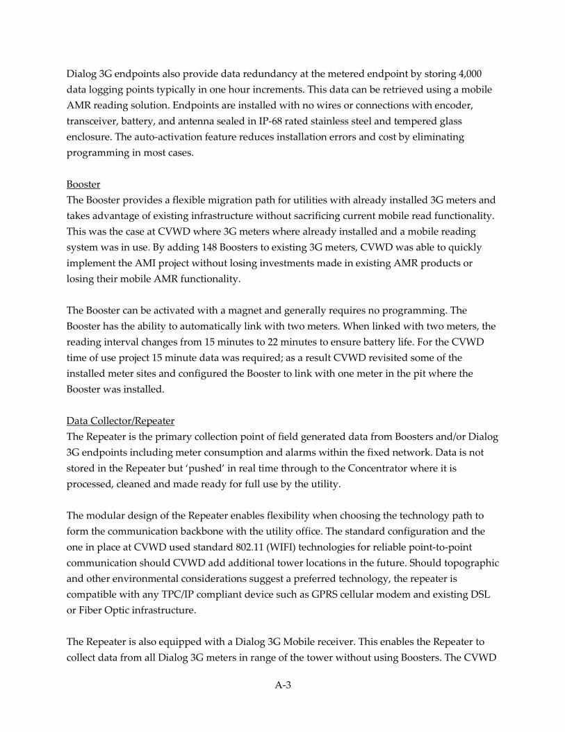
Dialog 3G endpoints also provide data redundancy at the metered endpoint by storing 4,000 data logging points typically in one hour increments. This data can be retrieved using a mobile AMR reading solution. Endpoints are installed with no wires or connections with encoder, transceiver, battery, and antenna sealed in IP-68 rated stainless steel and tempered glass enclosure. The auto-activation feature reduces installation errors and cost by eliminating programming in most cases. Booster The Booster provides a flexible migration path for utilities with already installed 3G meters and takes advantage of existing infrastructure without sacrificing current mobile read functionality. This was the case at CVWD where 3G meters where already installed and a mobile reading system was in use. By adding 148 Boosters to existing 3G meters, CVWD was able to quickly implement the AMI project without losing investments made in existing AMR products or losing their mobile AMR functionality. The Booster can be activated with a magnet and generally requires no programming. The Booster has the ability to automatically link with two meters. When linked with two meters, the reading interval changes from 15 minutes to 22 minutes to ensure battery life. For the CVWD time of use project 15 minute data was required; as a result CVWD revisited some of the installed meter sites and configured the Booster to link with one meter in the pit where the Booster was installed. Data Collector/Repeater The Repeater is the primary collection point of field generated data from Boosters and/or Dialog 3G endpoints including meter consumption and alarms within the fixed network. Data is not stored in the Repeater but ‘pushed’ in real time through to the Concentrator where it is processed, cleaned and made ready for full use by the utility. The modular design of the Repeater enables flexibility when choosing the technology path to form the communication backbone with the utility office. The standard configuration and the one in place at CVWD used standard 802.11 (WIFI) technologies for reliable point-to-point communication should CVWD add additional tower locations in the future. Should topographic and other environmental considerations suggest a preferred technology, the repeater is compatible with any TPC/IP compliant device such as GPRS cellular modem and existing DSL or Fiber Optic infrastructure. The Repeater is also equipped with a Dialog 3G Mobile receiver. This enables the Repeater to collect data from all Dialog 3G meters in range of the tower without using Boosters. The CVWD
A-3

Repeater received data from over 500 Dialog 3G endpoints without adding a Booster to existing mobile meter sets. Because the data for the study was limited to 148 meters these meters were not added to the system database. It is assumed that once the study is complete, these meters could be added and become part of larger AMI project should CVWD decide to move in that direction. Concentrator The AMI fixed network system employs a single PC Concentrator installed at the CVWD facility to integrate raw meter data into the meter data management system. The Concentrator ‘cleans’ incoming meter data and provides preliminary processing and optimization prior to access by the CVWD. The Concentrator provides local on-site data processing and a Microsoft SQL Database for data storage to provide 90 days of data redundancy as a safeguard against IP loss. Data is typically pushed through to the meter data management system every hour, during the CVWD installation period meter data was uploaded every 15 minutes because of the high level of interest from the CVWD staff in seeing data produced by the system. The Concentrator also decodes encrypted meter data, addresses error codes and provides data recovery stemming from slightly corrupted messages. Each Booster broadcast contains sixteen reading records and in many cases several readings can be salvaged from what would be considered a low quality transmission. Improvements in this process helped us achieve a high percentage of readings required by the TOU study Data Center and Hosted Meter Data Management (MDM) System CVWD is using a local software provider to create the graphical user interface for the TOU study. For the project the MDM System Data Center is providing CVWD a reading file every hour with readings for each meter in the study group. The MDM system software, database and application servers are located in a secure state-of-the-art Data Center which provides TCP/IP redundancy using three Tier 1 fiber optic connections to the internet with load balancing and automatic routing should one of more of the internet connections fail. The facility power is grouped using large uninterruptible power supply (UPS) units with short term battery backup and long term backup using a two megawatt generator with 1,500 gallons of fuel on-site. Temperature and humidity are controlled with redundant HVAC units.
A-4

The Meter Reading module provides a complete fixed network management solution presenting end users with meter data including data logging, daily readings, billing reads, revenue impact alerts and DMA (District Metered Areas) Leak Zone data processing results. Using tables, graphs, maps and a web based reporting system data is accessible to managers, utility employees and customer service representatives from any computer with internet access. Some of the key benefits of a hosted system are faster deployment times, no up-front license and limited infrastructure costs. Get up and running quickly was a pre-requisite of the TOU project. Meter Data Management System & Sample Data Main Meter Search Screen
A-5
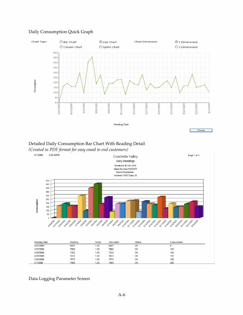
Daily Consumption Quick Graph
Detailed Daily Consumption Bar Chart With Reading Detail (Created in PDF format for easy email to end customers)
Data Logging Parameter Screen
A-6

Product & Installation Photos Booster in Pit Lid and Meter
A-7

Antennas and Low Loss Coax Cable On The Ground
Existing Tower Before Fixed Network Antennas Were Installed
A-8
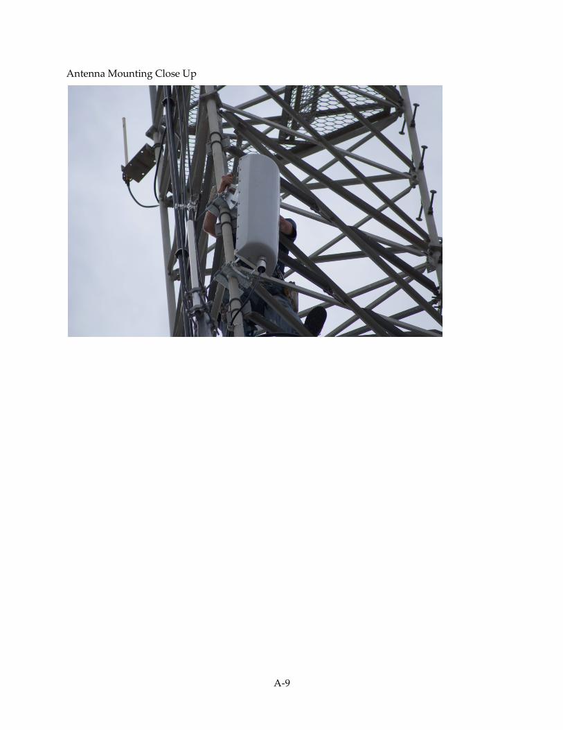
Antenna Mounting Close Up
A-9

Completed Antenna Installation On Existing Tower
A-10
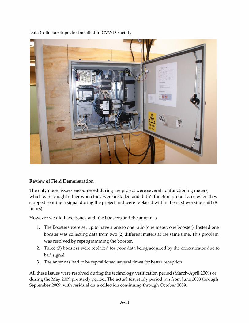
Data Collector/Repeater Installed In CVWD Facility
Review of Field Demonstration
The only meter issues encountered during the project were several nonfunctioning meters, which were caught either when they were installed and didn’t function properly, or when they stopped sending a signal during the project and were replaced within the next working shift (8 hours).
However we did have issues with the boosters and the antennas.
1. The Boosters were set up to have a one to one ratio (one meter, one booster). Instead one booster was collecting data from two (2) different meters at the same time. This problem was resolved by reprogramming the booster.
2. Three (3) boosters were replaced for poor data being acquired by the concentrator due to bad signal.
3. The antennas had to be repositioned several times for better reception.
All these issues were resolved during the technology verification period (March-April 2009) or during the May 2009 pre study period. The actual test study period ran from June 2009 through September 2009, with residual data collection continuing through October 2009.
A-11

Water Use Data Collection
The meters recorded and transmitted data in a predetermined format every 15 minutes. The format consisted of twelve columns. The columns were, from left to right, as follows: Meter Serial Number, Meter Electronic Number, Last Read, Read Date, Alternate Time, Factor, Extended Read, Meter Status, Location Number, Customer Name, and Group Name (see Appendix 2 for a description of how this data was used).
Meter Serial Number
Meter Electronic Number
Last Read
Read Date
Read Time
Factor Extended Read
Meter Status
Location Number
Account Number
Account Type
Account Group
6167740 5079687 775 4/30/2009 11:53 PM
10 7750 Leak 50610304801 50610304801 Business control-group
6167741 5079622 147 4/30/2009 11:56 PM
10 1470 OK 50610300101 50610300101 Business control-group
For each meter, the 15 minute interval data looks like this example for March 10th for account 5410805:
3/10/2009 23:55 1 5410805 48869
3/10/2009 23:40 2 5410805 48869
3/10/2009 23:25 3 5410805 48869
3/10/2009 23:10 4 5410805 48869
3/10/2009 22:55 5 5410805 48869
3/10/2009 22:40 6 5410805 48869
3/10/2009 22:25 7 5410805 48869
3/10/2009 22:10 8 5410805 48869
3/10/2009 21:55 9 5410805 48869
3/10/2009 21:40 10 5410805 48869
3/10/2009 21:25 11 5410805 48869
3/10/2009 21:10 12 5410805 48869
3/10/2009 20:55 13 5410805 48869
3/10/2009 20:40 14 5410805 48869
3/10/2009 20:25 15 5410805 48869
3/10/2009 20:10 16 5410805 48869
3/10/2009 19:55 17 5410805 48869
A-12
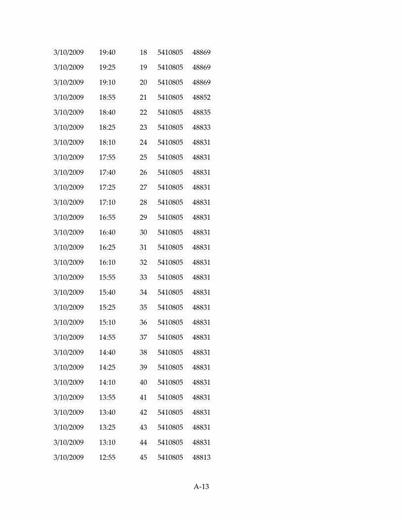
3/10/2009 19:40 18 5410805 48869
3/10/2009 19:25 19 5410805 48869
3/10/2009 19:10 20 5410805 48869
3/10/2009 18:55 21 5410805 48852
3/10/2009 18:40 22 5410805 48835
3/10/2009 18:25 23 5410805 48833
3/10/2009 18:10 24 5410805 48831
3/10/2009 17:55 25 5410805 48831
3/10/2009 17:40 26 5410805 48831
3/10/2009 17:25 27 5410805 48831
3/10/2009 17:10 28 5410805 48831
3/10/2009 16:55 29 5410805 48831
3/10/2009 16:40 30 5410805 48831
3/10/2009 16:25 31 5410805 48831
3/10/2009 16:10 32 5410805 48831
3/10/2009 15:55 33 5410805 48831
3/10/2009 15:40 34 5410805 48831
3/10/2009 15:25 35 5410805 48831
3/10/2009 15:10 36 5410805 48831
3/10/2009 14:55 37 5410805 48831
3/10/2009 14:40 38 5410805 48831
3/10/2009 14:25 39 5410805 48831
3/10/2009 14:10 40 5410805 48831
3/10/2009 13:55 41 5410805 48831
3/10/2009 13:40 42 5410805 48831
3/10/2009 13:25 43 5410805 48831
3/10/2009 13:10 44 5410805 48831
3/10/2009 12:55 45 5410805 48813
A-13
3/10/2009 12:40 46 5410805 48795
3/10/2009 12:25 47 5410805 48795
3/10/2009 12:10 48 5410805 48795
3/10/2009 11:55 49 5410805 48795
3/10/2009 11:40 50 5410805 48795
3/10/2009 11:25 51 5410805 48795
3/10/2009 11:10 52 5410805 48795
3/10/2009 10:55 53 5410805 48795
3/10/2009 10:40 54 5410805 48795
3/10/2009 10:25 55 5410805 48795
3/10/2009 10:10 56 5410805 48795
3/10/2009 9:55 57 5410805 48795
3/10/2009 9:40 58 5410805 48795
3/10/2009 9:25 59 5410805 48795
3/10/2009 9:10 60 5410805 48795
3/10/2009 8:55 61 5410805 48795
3/10/2009 8:40 62 5410805 48794
3/10/2009 8:25 63 5410805 48793
3/10/2009 8:10 64 5410805 48793
3/10/2009 7:55 65 5410805 48793
3/10/2009 7:40 66 5410805 48792
3/10/2009 7:25 67 5410805 48790
3/10/2009 7:10 68 5410805 48789
3/10/2009 6:55 69 5410805 48789
3/10/2009 6:40 70 5410805 48789
3/10/2009 6:25 71 5410805 48789
3/10/2009 6:10 72 5410805 48789
3/10/2009 5:55 73 5410805 48789
A-14
3/10/2009 5:40 74 5410805 48789
3/10/2009 5:25 75 5410805 48789
3/10/2009 5:10 76 5410805 48789
3/10/2009 4:55 77 5410805 48789
3/10/2009 4:40 78 5410805 48789
3/10/2009 4:25 79 5410805 48789
3/10/2009 4:10 80 5410805 48789
3/10/2009 3:55 81 5410805 48789
3/10/2009 3:40 82 5410805 48789
3/10/2009 3:25 83 5410805 48789
3/10/2009 3:10 84 5410805 48789
3/10/2009 2:55 85 5410805 48789
3/10/2009 2:40 86 5410805 48789
3/10/2009 2:25 87 5410805 48789
3/10/2009 2:10 88 5410805 48789
3/10/2009 1:55 89 5410805 48789
3/10/2009 1:40 90 5410805 48789
3/10/2009 1:25 91 5410805 48789
3/10/2009 1:10 92 5410805 48789
3/10/2009 0:55 93 5410805 48789
3/10/2009 0:40 94 5410805 48789
3/10/2009 0:25 95 5410805 48789
3/10/2009 0:10 96 5410805 48789
A-15

APPENDIX B: Data and Statistical Analysis
Jordan David House, M.S., Ph.D. Candidate
University of Massachusetts Amherst
Department of Kinesiology
Format of Data
The data were recorded in a predetermined format. The format consisted of twelve columns. The columns were, from left to right, as follows: Meter Serial Number, Meter Electronic Number, Last Read, Read Date, Read Time, Factor, Extended Read, Meter Status, Location Number, Account Number, Account Type, and Account Group.
Meter Serial Number
Meter Electronic Number
Last Read
Read Date
Read Time
Factor Extended Read
Meter Status
Location Number
Account Number
Account Group
6167740 5079687 775 4/30/2009 11:53 PM
10 7750 Leak 50610304801 50610304801 Control-group
6167741 5079622 147 4/30/2009 11:56 PM
10 1470 OK 50610300101 50610300101 Control-group
Based on the original format, the data were sorted according to: Account Number, Group Name, Meter Serial Number, Read Date, and finally Read Time respectively. Data reduction was performed in order to minimize the number of extraneous variables, resulting in a data set that consisted of eight columns. These eight columns read, from left to right: Meter Number, Read Date, Read Time (rounded to the nearest hour), Read Value (in cubic feet), Read Value (cubic feet converted to gallons), the dependent variable of interest (such as Total Monthly Water Use, Total On-Peak Water Use, etc.), Group Name (renamed from Account Number), and finally Group (renamed from Account Group). The data reduction process was performed for all groups (Residential, Business, and Irrigation) and groups (Control and Intervention), and this format was used to calculate all dependent variables of interest.
B-1
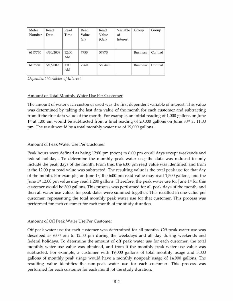
Meter Number
Read Date
Read Time
Read Value (cf)
Read Value (Gal)
Variable of Interest
Group Group
6167740 4/30/2009 12:00 AM
7750 57970 Business Control
6167740 5/1/2009 1:00 AM
7760 58044.8 Business Control
Dependent Variables of Interest
Amount of Total Monthly Water Use Per Customer
The amount of water each customer used was the first dependent variable of interest. This value was determined by taking the last data value of the month for each customer and subtracting from it the first data value of the month. For example, an initial reading of 1,000 gallons on June 1st at 1:00 am would be subtracted from a final reading of 20,000 gallons on June 30th at 11:00 pm. The result would be a total monthly water use of 19,000 gallons.
Amount of Peak Water Use Per Customer
Peak hours were defined as being 12:00 pm (noon) to 6:00 pm on all days except weekends and federal holidays. To determine the monthly peak water use, the data was reduced to only include the peak days of the month. From this, the 6:00 pm read value was identified, and from it the 12:00 pm read value was subtracted. The resulting value is the total peak use for that day of the month. For example, on June 1st, the 6:00 pm read value may read 1,500 gallons, and the June 1st 12:00 pm value may read 1,200 gallons. Therefore, the peak water use for June 1st for this customer would be 300 gallons. This process was performed for all peak days of the month, and then all water use values for peak dates were summed together. This resulted in one value per customer, representing the total monthly peak water use for that customer. This process was performed for each customer for each month of the study duration.
Amount of Off Peak Water Use Per Customer
Off peak water use for each customer was determined for all months. Off peak water use was described as 6:00 pm to 12:00 pm during the weekdays and all day during weekends and federal holidays. To determine the amount of off peak water use for each customer, the total monthly water use value was obtained, and from it the monthly peak water use value was subtracted. For example, a customer with 19,000 gallons of total monthly usage and 5,000 gallons of monthly peak usage would have a monthly nonpeak usage of 14,000 gallons. The resulting value identifies the non-peak water use for each customer. This process was performed for each customer for each month of the study duration.
B-2
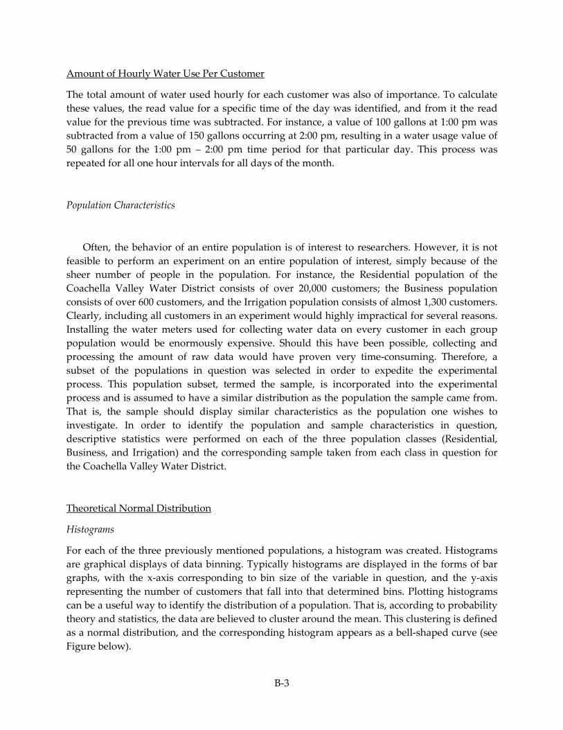
Amount of Hourly Water Use Per Customer
The total amount of water used hourly for each customer was also of importance. To calculate these values, the read value for a specific time of the day was identified, and from it the read value for the previous time was subtracted. For instance, a value of 100 gallons at 1:00 pm was subtracted from a value of 150 gallons occurring at 2:00 pm, resulting in a water usage value of 50 gallons for the 1:00 pm – 2:00 pm time period for that particular day. This process was repeated for all one hour intervals for all days of the month.
Population Characteristics
Often, the behavior of an entire population is of interest to researchers. However, it is not feasible to perform an experiment on an entire population of interest, simply because of the sheer number of people in the population. For instance, the Residential population of the Coachella Valley Water District consists of over 20,000 customers; the Business population consists of over 600 customers, and the Irrigation population consists of almost 1,300 customers. Clearly, including all customers in an experiment would highly impractical for several reasons. Installing the water meters used for collecting water data on every customer in each group population would be enormously expensive. Should this have been possible, collecting and processing the amount of raw data would have proven very time-consuming. Therefore, a subset of the populations in question was selected in order to expedite the experimental process. This population subset, termed the sample, is incorporated into the experimental process and is assumed to have a similar distribution as the population the sample came from. That is, the sample should display similar characteristics as the population one wishes to investigate. In order to identify the population and sample characteristics in question, descriptive statistics were performed on each of the three population classes (Residential, Business, and Irrigation) and the corresponding sample taken from each class in question for the Coachella Valley Water District.
Theoretical Normal Distribution
Histograms
For each of the three previously mentioned populations, a histogram was created. Histograms are graphical displays of data binning. Typically histograms are displayed in the forms of bar graphs, with the x-axis corresponding to bin size of the variable in question, and the y-axis representing the number of customers that fall into that determined bins. Plotting histograms can be a useful way to identify the distribution of a population. That is, according to probability theory and statistics, the data are believed to cluster around the mean. This clustering is defined as a normal distribution, and the corresponding histogram appears as a bell-shaped curve (see Figure below).
B-3
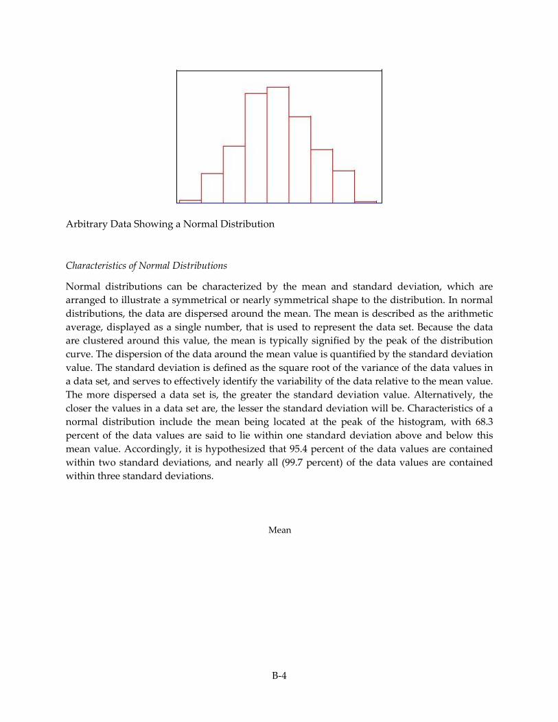
Arbitrary Data Showing a Normal Distribution
Characteristics of Normal Distributions
Normal distributions can be characterized by the mean and standard deviation, which are arranged to illustrate a symmetrical or nearly symmetrical shape to the distribution. In normal distributions, the data are dispersed around the mean. The mean is described as the arithmetic average, displayed as a single number, that is used to represent the data set. Because the data are clustered around this value, the mean is typically signified by the peak of the distribution curve. The dispersion of the data around the mean value is quantified by the standard deviation value. The standard deviation is defined as the square root of the variance of the data values in a data set, and serves to effectively identify the variability of the data relative to the mean value. The more dispersed a data set is, the greater the standard deviation value. Alternatively, the closer the values in a data set are, the lesser the standard deviation will be. Characteristics of a normal distribution include the mean being located at the peak of the histogram, with 68.3 percent of the data values are said to lie within one standard deviation above and below this mean value. Accordingly, it is hypothesized that 95.4 percent of the data values are contained within two standard deviations, and nearly all (99.7 percent) of the data values are contained within three standard deviations.
Mean
B-4
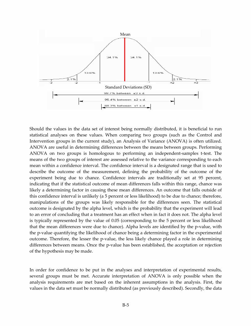
Should the values in the data set of interest being normally distributed, it is beneficial to run statistical analyses on these values. When comparing two groups (such as the Control and Intervention groups in the current study), an Analysis of Variance (ANOVA) is often utilized. ANOVA are useful in determining differences between the means between groups. Performing ANOVA on two groups is homologous to performing an independent-samples t-test. The means of the two groups of interest are assessed relative to the variance corresponding to each mean within a confidence interval. The confidence interval is a designated range that is used to describe the outcome of the measurement, defining the probability of the outcome of the experiment being due to chance. Confidence intervals are traditionally set at 95 percent, indicating that if the statistical outcome of mean differences falls within this range, chance was likely a determining factor in causing these mean differences. An outcome that falls outside of this confidence interval is unlikely (a 5 percent or less likelihood) to be due to chance; therefore, manipulations of the groups was likely responsible for the differences seen. The statistical outcome is designated by the alpha level, which is the probability that the experiment will lead to an error of concluding that a treatment has an effect when in fact it does not. The alpha level is typically represented by the value of 0.05 (corresponding to the 5 percent or less likelihood that the mean differences were due to chance). Alpha levels are identified by the p-value, with the p-value quantifying the likelihood of chance being a determining factor in the experimental outcome. Therefore, the lesser the p-value, the less likely chance played a role in determining differences between means. Once the p-value has been established, the acceptation or rejection of the hypothesis may be made.
In order for confidence to be put in the analyses and interpretation of experimental results, several groups must be met. Accurate interpretation of ANOVA is only possible when the analysis requirements are met based on the inherent assumptions in the analysis. First, the values in the data set must be normally distributed (as previously described). Secondly, the data
Standard Deviations (SD)
Mean
B-5
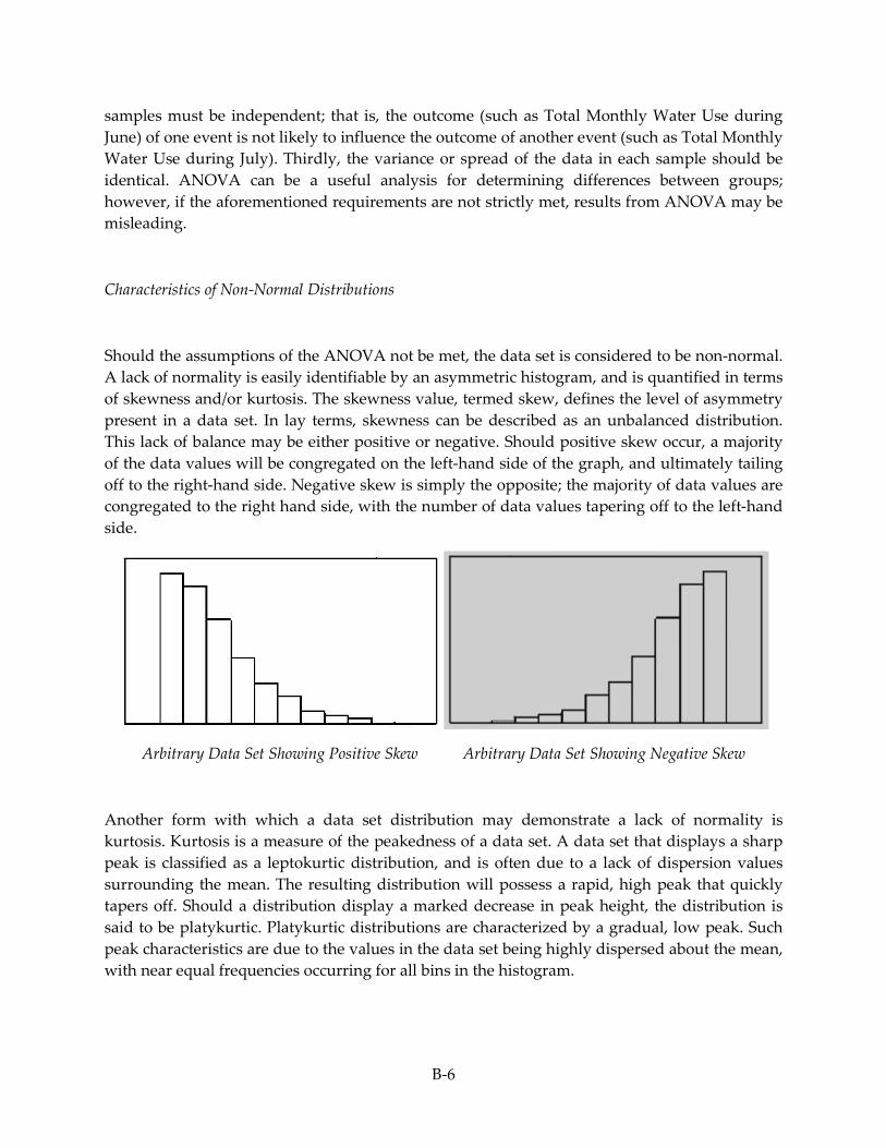
samples must be independent; that is, the outcome (such as Total Monthly Water Use during June) of one event is not likely to influence the outcome of another event (such as Total Monthly Water Use during July). Thirdly, the variance or spread of the data in each sample should be identical. ANOVA can be a useful analysis for determining differences between groups; however, if the aforementioned requirements are not strictly met, results from ANOVA may be misleading.
Characteristics of Non-Normal Distributions
Should the assumptions of the ANOVA not be met, the data set is considered to be non-normal. A lack of normality is easily identifiable by an asymmetric histogram, and is quantified in terms of skewness and/or kurtosis. The skewness value, termed skew, defines the level of asymmetry present in a data set. In lay terms, skewness can be described as an unbalanced distribution. This lack of balance may be either positive or negative. Should positive skew occur, a majority of the data values will be congregated on the left-hand side of the graph, and ultimately tailing off to the right-hand side. Negative skew is simply the opposite; the majority of data values are congregated to the right hand side, with the number of data values tapering off to the left-hand side.
Arbitrary Data Set Showing Positive Skew Arbitrary Data Set Showing Negative Skew
Another form with which a data set distribution may demonstrate a lack of normality is kurtosis. Kurtosis is a measure of the peakedness of a data set. A data set that displays a sharp peak is classified as a leptokurtic distribution, and is often due to a lack of dispersion values surrounding the mean. The resulting distribution will possess a rapid, high peak that quickly tapers off. Should a distribution display a marked decrease in peak height, the distribution is said to be platykurtic. Platykurtic distributions are characterized by a gradual, low peak. Such peak characteristics are due to the values in the data set being highly dispersed about the mean, with near equal frequencies occurring for all bins in the histogram.
B-6

Arbitrary Data Showing Leptokurtic Distribution Arbitrary Data Showing Platykurtic Distribution
It is important to note that though normal populations are theoretical, it is possible for them to exist. Oftentimes, recruiting a large number of participants to increase sample size will move the distribution to being more normal. However, it remains a possibility that a normal distribution will not be achieved. Non-normal distributions may possess one or many of the aforementioned characteristics. Should such characteristics be present in a distribution, traditional measures that summarize the data set should not be used. If a distribution is normal, then the mean can be an accurate representation of the values in the data set, and comparing means among groups for significant differences using ANOVA may be appropriate. However, if the distribution of the data is not normal, means and significance values for differences between groups can be misleading, as they poorly represent the values in a data set.
Distribution of Study Populations and Samples
Three population classes were assessed in the current study; Residential (over 20,000 customers), Business (over 600 customers), and Irrigation (almost 1,300 customers). As previously described, incorporating all such customers into the current study would be challenging. Therefore, samples were drawn from each population within a one mile radius of the CVWD field office in the city of Palm Desert due to telemetry issues (see Appendix 1). Sample sizes included 102 customers from the Residential class, 22 customers from the Business class, and 22 customers from the Irrigation class. In order to determine if the samples were accurate representations of the populations drawn from, histograms were made identifying the distributions of both the class population (as a line graph, corresponding to units on the left-hand y-axis) and the class sample (as a bar graph, corresponding to the units on the right-hand y-axis). For the following histograms, the bin width was arbitrarily set to include 10,000 customers.
B-7

Residential Class Characteristics
Population Sample
Number (n) 20953 102
Mean 19793 25600
Standard Deviation 31788 16451
Median 9724 21254
Skewness 14.076 1.256
St Error of Skewness 0.017 0.237
Kurtosis 462.54 2.148
Std Error Kurtosis 0.034 0.469
B-8

Business Class Characteristics
Population Sample
Number (n) 657 22
Mean 27081 26640
Standard Deviation 59271 39892
Median 9724 1275
Skewness 6.74 2.649
St Error of Skewness 0.095 0.491
Kurtosis 58.88 6.901
Std Error Kurtosis 0.19 0.95
Irrigation Class Characteristics
B-9

It is apparent that, for all classes, the frequency distribution of the samples generally agrees with the distribution of the population. This is due to the fact that, for each class, the characteristics of the sample histogram follows the characteristics population histogram. With this said, it is feasible to conclude that the samples drawn are reasonable representations of the populations originated from. Therefore, changes in behavior seen in our sample group can theoretically be hypothesized to occur in the population the sample was drawn from, due to similar profile characteristics.
Population Sample
Number (n) 1299 22
Mean 197595 62803
Standard Deviation 262353 95038
Median 79662 35960
Skewness 1.906 2.897
St Error of Skewness 0.068 0.491
Kurtosis 3.768 10.196
Std Error Kurtosis 0.136 0.953
B-10

One will quickly note that though the class samples display similar profile characteristics to the populations, there exists a definite lack of normality in the distributions plotted. In order to identify the level of non-normality present for each class histogram, values for skewness and kurtosis have been reported. Should a normal distribution be present, kurtosis and skewness values will be 0, indicating symmetry in the distribution. Clearly, there is kurtosis as well as skewness occurring in the population and sample data sets. All classes demonstrate positive skew, with a majority of the data values congregating to the left-hand side of the graph and dispersing to the right-hand side of the graph. The skewness of the data due to the unique dispersion provides complications in attempts to summarize the data, analyze effects of treatment, and interpret these results using traditional measures. The non-normality of the current data sets requires that techniques used to investigate parametric (normally distributed) data such as mean, standard deviation, and ANOVA must be substituted with nonparametric (non-normal) analyses in order to avoid misleading outcomes.
Total Monthly, On-Peak, and Off Peak Water Usage
For the months the study was performed (June, July, August, September), nonparametric statistics were utilized to generate the dependent variables of interest. The dependent variables of interest included Total Monthly, On-Peak, and Off Peak water usage for the months of June, July, August, and September. Specifically, median values were generated for all such dependent variables during these time periods. The median is a numeric value from a data set that evenly divides the data into upper and lower halves. Medians are often used in place of means when the data is skewed. The positive skewness of the current data suggests that while a majority of the customers in both population and samples are congregated towards low Monthly Water Use values, there exist customers that use a much greater amount of water during the month. Such high-consumption customers serve to artificially inflate the mean of the data to the degree that the mean is no longer representative of the data majority.
By using a nonparametric statistic such as the median to represent data for the variable of interest (Total Monthly, On-Peak, and Off Peak Water Usage), the effect of high-consumption customers can be minimized if there are few high-consumption customers. Based on the frequency histograms generated, it is evident that a majority of the customers in all customer groups consume low amounts of water. Per the distribution characteristics of the customer populations and samples, it is essential that a nonparametric statistical analysis be utilized in order to evaluate differences observed between groups. For the current study, a Mann-Whitney U test was used as a nonparametric alternative to the parametric ANOVA.
Mann-Whitney U Test
B-11

The Mann-Whitney U test begins with a null hypothesis, which states that there will be no differences in the distributions of data values between the Intervention and Control groups for a particular dependent variable and group. The alternative hypothesis is that there will be a difference in distribution between the Intervention and Control groups. In order to determine differences in distributions between groups, the Mann-Whitney U test uses an ordinal (ranking) scale. For a particular dependent variable (for instance, Total Monthly Water Use) for a particular month (for instance, June), data from both groups are combined. Then, each data point is ranked and assigned a ranking value. The rank values are then summed together for each group, and a single number is generated for each group. This number is referred to as the U statistic.
Should a large difference exist in the distributions between the two groups tested, this will be evident by the distribution for one group (the Intervention group, for example) clustering towards lower rank values and the distribution for the other group (the Control group, for example). Should the sample sizes be large (n > 20), the Mann-Whitney U statistic approaches a normal shape. When this occurs, a z-score is generated. The z-score defines where the U-value occurs within a normal distribution, and therefore comes to represent the U-value. This z-score identifies how many standard deviations away from the mean the U-value lays. According to the normal distribution, the further away from the mean a value lays the greater standard deviation that value will have. Therefore, the greater the z-score, the greater the standard deviation, and the less likely this outcome would occur due to chance. The likelihood of an outcome happening due to chance is identified by the confidence interval, which in this study was set to 95 percent. In other words, should differences between two groups be seen to occur outside this confidence interval, there is a 5 percent or less likelihood that chance caused these differences. An alpha level, set at 0.05, was utilized in the study as a level of significance. That is, should differences exist in the distribution between two groups, these differences will be assigned a z-score. If this z-score is large enough to occur outside the confidence interval of 95 percent, there is a 5 percent or less likelihood that chance caused these differences between groups. In this instance, the null hypothesis would be rejected, indicating that the differences between groups were likely a cause of the treatment the groups received.
Data Summaries
A Mann-Whitney U test was employed to compare the distribution of the Intervention group versus the distribution of the Control group for all combinations of customer classes (Residential, Business, and Irrigation) for the duration of the study (June, July, August, and September) for the dependent variables of interest (Total Monthly, On-Peak, and Off Peak water
B-12
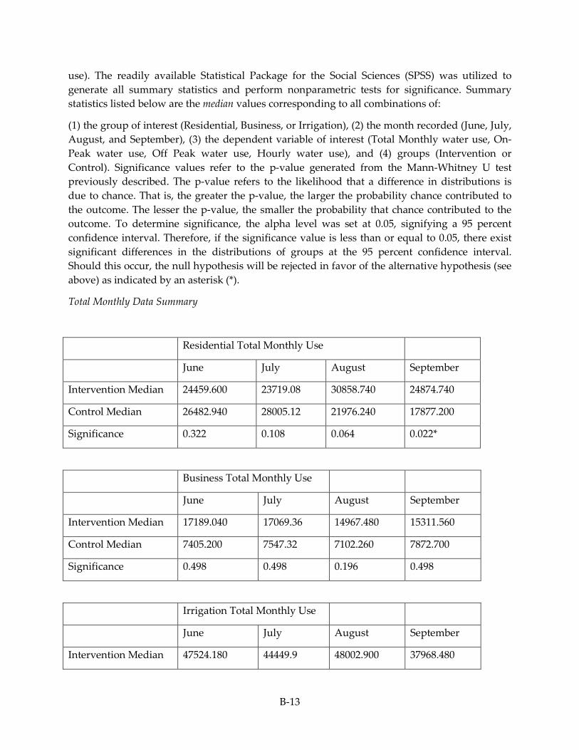
use). The readily available Statistical Package for the Social Sciences (SPSS) was utilized to generate all summary statistics and perform nonparametric tests for significance. Summary statistics listed below are the median values corresponding to all combinations of:
(1) the group of interest (Residential, Business, or Irrigation), (2) the month recorded (June, July, August, and September), (3) the dependent variable of interest (Total Monthly water use, On-Peak water use, Off Peak water use, Hourly water use), and (4) groups (Intervention or Control). Significance values refer to the p-value generated from the Mann-Whitney U test previously described. The p-value refers to the likelihood that a difference in distributions is due to chance. That is, the greater the p-value, the larger the probability chance contributed to the outcome. The lesser the p-value, the smaller the probability that chance contributed to the outcome. To determine significance, the alpha level was set at 0.05, signifying a 95 percent confidence interval. Therefore, if the significance value is less than or equal to 0.05, there exist significant differences in the distributions of groups at the 95 percent confidence interval. Should this occur, the null hypothesis will be rejected in favor of the alternative hypothesis (see above) as indicated by an asterisk (*).
Total Monthly Data Summary
Residential Total Monthly Use
June July August September
Intervention Median 24459.600 23719.08 30858.740 24874.740
Control Median 26482.940 28005.12 21976.240 17877.200
Significance 0.322 0.108 0.064 0.022*
Business Total Monthly Use
June July August September
Intervention Median 17189.040 17069.36 14967.480 15311.560
Control Median 7405.200 7547.32 7102.260 7872.700
Significance 0.498 0.498 0.196 0.498
Irrigation Total Monthly Use
June July August September
Intervention Median 47524.180 44449.9 48002.900 37968.480
B-13

Control Median 29377.700 56429.12 58119.600 66220.440
Significance 0.510 0.360 0.429 0.166
On-Peak Data Summary
Residential On-Peak Use
June July August September
Intervention Median 1765.280 2071.96 1578.280 1750.320
Control Median 5509.020 5258.44 6451.500 4817.120
Significance 0.000* 0.000* 0.000* 0.000*
Business On-Peak Use
June July August September
Intervention Median 5430.48 5684.8 5228.520 5198.600
Control Median 3998.06 4121.48 3466.980 2588.080
Significance 0.667 0.712 0.580 0.356
Irrigation On-Peak Use
June July August September
Intervention Median 5819.44 7218.2 7954.980 6780.620
Control Median 276.76 583.44 628.320 1496.000
Significance 0.203 0.056 0.145 0.305
Off Peak Data Summary
Residential Off Peak Use
June July August September
B-14
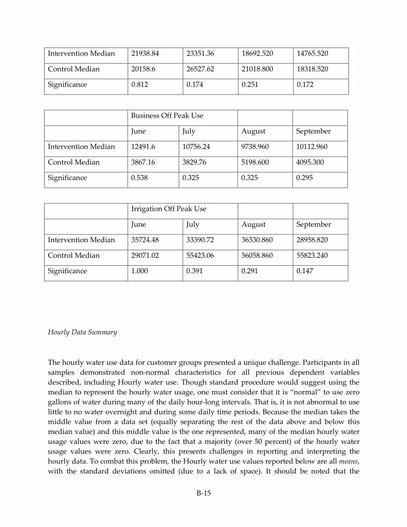
Intervention Median 21938.84 23351.36 18692.520 14765.520
Control Median 20158.6 26527.62 21018.800 18318.520
Significance 0.812 0.174 0.251 0.172
Business Off Peak Use
June July August September
Intervention Median 12491.6 10756.24 9738.960 10112.960
Control Median 3867.16 3829.76 5198.600 4095.300
Significance 0.538 0.325 0.325 0.295
Irrigation Off Peak Use
June July August September
Intervention Median 35724.48 33390.72 36330.860 28958.820
Control Median 29071.02 55423.06 56058.860 55823.240
Significance 1.000 0.391 0.291 0.147
Hourly Data Summary
The hourly water use data for customer groups presented a unique challenge. Participants in all samples demonstrated non-normal characteristics for all previous dependent variables described, including Hourly water use. Though standard procedure would suggest using the median to represent the hourly water usage, one must consider that it is “normal” to use zero gallons of water during many of the daily hour-long intervals. That is, it is not abnormal to use little to no water overnight and during some daily time periods. Because the median takes the middle value from a data set (equally separating the rest of the data above and below this median value) and this middle value is the one represented, many of the median hourly water usage values were zero, due to the fact that a majority (over 50 percent) of the hourly water usage values were zero. Clearly, this presents challenges in reporting and interpreting the hourly data. To combat this problem, the Hourly water use values reported below are all means, with the standard deviations omitted (due to a lack of space). It should be noted that the
B-15

standard deviations accompanying the means in the following tables were very high, indicating a large spread of the data. Therefore, interpret the hourly results with some reservation. Though they are not misleading per se, the wide distributions of these data indicate that the following means are not the most accurate representation of the sample of origin.
B-16

Residential Hourly
June June July July August August September September
Intervention Control Intervention Control Intervention Control Intervention Control
12:00 AM
38.99 12.86 45.88 14.90 53.28 16.12 36.76 8.97
1:00 AM 12.06 19.64 17.22 21.10 20.04 20.09 19.95 17.21
2:00 AM 10.85 13.88 21.15 16.60 14.99 20.88 9.36 16.44
3:00 AM 11.49 7.35 13.62 8.10 11.44 7.66 9.75 7.19
4:00 AM 19.36 4.99 10.84 12.74 22.78 13.01 9.63 12.65
5:00 AM 21.19 14.89 15.46 17.81 16.38 16.54 16.81 15.61
6:00 AM 69.01 28.27 53.42 26.12 50.88 20.54 34.29 17.73
7:00 AM 62.15 31.35 64.67 34.39 60.63 29.96 64.51 31.71
8:00 AM 51.88 49.41 55.65 49.15 55.78 55.02 44.24 54.24
9:00 AM 75.98 90.37 63.12 89.55 65.55 100.94 69.03 89.07
10:00 AM
55.53 102.90 50.80 93.63 50.13 79.41 34.53 66.65
11:00 AM
32.69 61.51 30.19 58.41 26.63 44.33 22.07 42.51
12:00 PM 53.35 40.02 41.29 51.88 33.33 51.08 25.71 36.42
1:00 PM 34.25 57.68 25.69 65.82 20.08 72.25 15.25 64.57
2:00 PM 27.16 62.17 27.11 65.49 25.18 63.38 20.35 48.68
3:00 PM 30.58 34.50 27.96 35.95 26.02 34.86 20.18 29.75
4:00 PM 25.52 79.00 23.38 65.07 25.89 58.39 22.27 48.71
5:00 PM 23.58 53.69 26.61 37.32 30.37 31.06 31.44 31.86
6:00 PM 44.89 95.14 45.50 104.32 46.72 122.42 38.09 104.86
7:00 PM 53.88 63.02 54.77 72.48 51.96 76.19 45.82 62.79
8:00 PM 60.15 42.94 65.93 37.44 69.01 49.45 58.89 37.16
9:00 PM 63.74 32.55 49.74 37.15 47.02 39.77 30.12 31.69
10:00 PM 23.99 24.70 34.27 22.14 27.36 21.42 26.98 21.78
11:00 PM 33.02 18.58 28.05 17.59 27.16 15.55 19.07 12.74
B-17

Business Hourly
June June July July August August September September
Intervention Control Intervention Control Intervention Control Intervention Control
12:00 AM 9.07 32.60 23.29 22.20 9.33 7.08 5.43 29.41
1:00 AM 10.95 18.43 20.81 22.17 9.63 7.44 7.94 18.15
2:00 AM 7.95 20.38 19.93 21.86 10.06 9.37 7.41 16.99
3:00 AM 5.95 15.05 18.43 19.58 9.23 7.42 7.85 14.06
4:00 AM 78.49 18.95 87.79 20.43 79.79 10.39 63.15 18.34
5:00 AM 19.91 17.42 20.26 21.32 22.21 8.29 13.93 16.32
6:00 AM 17.35 17.67 16.96 19.82 18.35 8.20 16.31 17.32
7:00 AM 10.23 32.09 27.09 30.28 34.51 20.74 31.24 27.73
8:00 AM 31.02 28.63 30.25 31.97 29.01 20.47 25.84 33.18
9:00 AM 28.07 67.04 34.98 74.76 37.38 59.11 31.36 59.40
10:00 AM 36.45 79.98 37.79 79.47 35.71 76.02 31.80 70.14
11:00 AM 37.12 89.93 41.28 81.98 40.61 74.25 36.07 69.51
12:00 PM 48.61 83.93 47.78 82.66 52.82 66.98 49.78 71.09
1:00 PM 36.75 88.40 38.07 74.57 44.39 66.27 35.95 69.07
2:00 PM 44.44 80.58 45.22 76.03 48.15 61.67 43.74 84.08
3:00 PM 41.52 76.13 44.34 73.67 47.47 65.60 43.92 67.82
4:00 PM 30.81 88.46 30.64 81.21 33.82 69.43 29.09 71.56
5:00 PM 20.36 76.76 24.41 63.09 23.16 53.63 24.30 51.79
6:00 PM 83.84 31.18 89.64 37.83 83.75 20.87 66.77 28.49
7:00 PM 13.15 24.22 14.51 26.67 13.36 11.62 11.60 21.27
8:00 PM 28.17 26.34 28.79 24.66 30.31 12.29 26.17 21.75
9:00 PM 9.51 23.07 21.93 20.63 17.70 12.93 11.25 20.15
10:00 PM 8.36 20.34 21.28 23.43 13.65 11.74 12.34 19.52
11:00 PM 70.20 21.77 88.88 20.62 70.65 8.84 52.75 20.34
Irrigation Hourly
June June July July August August September September
B-18
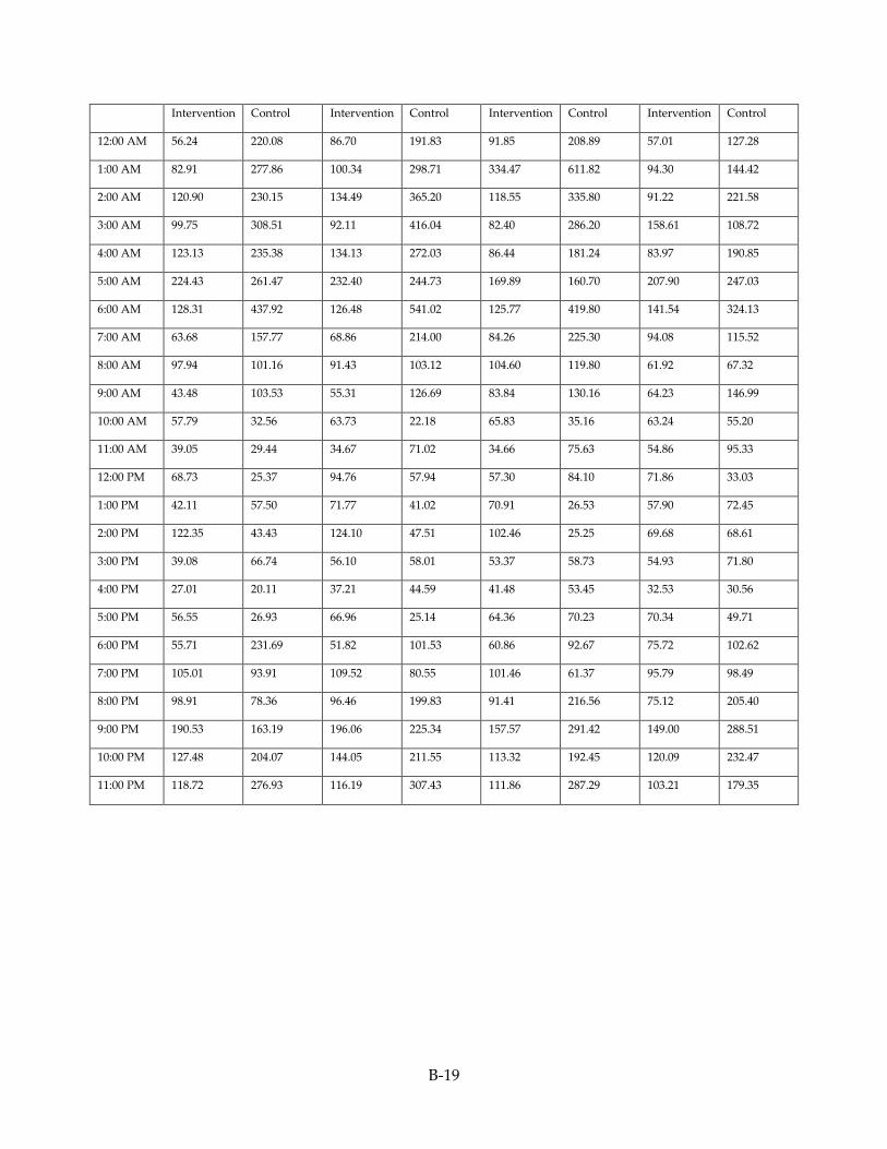
Intervention Control Intervention Control Intervention Control Intervention Control
12:00 AM 56.24 220.08 86.70 191.83 91.85 208.89 57.01 127.28
1:00 AM 82.91 277.86 100.34 298.71 334.47 611.82 94.30 144.42
2:00 AM 120.90 230.15 134.49 365.20 118.55 335.80 91.22 221.58
3:00 AM 99.75 308.51 92.11 416.04 82.40 286.20 158.61 108.72
4:00 AM 123.13 235.38 134.13 272.03 86.44 181.24 83.97 190.85
5:00 AM 224.43 261.47 232.40 244.73 169.89 160.70 207.90 247.03
6:00 AM 128.31 437.92 126.48 541.02 125.77 419.80 141.54 324.13
7:00 AM 63.68 157.77 68.86 214.00 84.26 225.30 94.08 115.52
8:00 AM 97.94 101.16 91.43 103.12 104.60 119.80 61.92 67.32
9:00 AM 43.48 103.53 55.31 126.69 83.84 130.16 64.23 146.99
10:00 AM 57.79 32.56 63.73 22.18 65.83 35.16 63.24 55.20
11:00 AM 39.05 29.44 34.67 71.02 34.66 75.63 54.86 95.33
12:00 PM 68.73 25.37 94.76 57.94 57.30 84.10 71.86 33.03
1:00 PM 42.11 57.50 71.77 41.02 70.91 26.53 57.90 72.45
2:00 PM 122.35 43.43 124.10 47.51 102.46 25.25 69.68 68.61
3:00 PM 39.08 66.74 56.10 58.01 53.37 58.73 54.93 71.80
4:00 PM 27.01 20.11 37.21 44.59 41.48 53.45 32.53 30.56
5:00 PM 56.55 26.93 66.96 25.14 64.36 70.23 70.34 49.71
6:00 PM 55.71 231.69 51.82 101.53 60.86 92.67 75.72 102.62
7:00 PM 105.01 93.91 109.52 80.55 101.46 61.37 95.79 98.49
8:00 PM 98.91 78.36 96.46 199.83 91.41 216.56 75.12 205.40
9:00 PM 190.53 163.19 196.06 225.34 157.57 291.42 149.00 288.51
10:00 PM 127.48 204.07 144.05 211.55 113.32 192.45 120.09 232.47
11:00 PM 118.72 276.93 116.19 307.43 111.86 287.29 103.21 179.35
B-19


![Octave Water Meter - RMC Water Control Valves · Maximum Cable Length* 500 [meter] Maximum Applied Voltage 35 [Vdc] ... Octave Water Meter Installation Manual](https://img.dokumen.tips/doc/110x75/5b0c90c77f8b9a6a6b8c7f4a/octave-water-meter-rmc-water-control-cable-length-500-meter-maximum-applied.jpg)