Embed Size (px)
Citation preview

1
Time-Domain System Analysis
M. J. Roberts - All Rights Reserved. Edited by Dr. Robert Akl
1
Continuous Time
M. J. Roberts - All Rights Reserved. Edited by Dr. Robert Akl 2
Impulse Response Let a system be described by a2 ′′y t( ) + a1 ′y t( ) + a0 y t( ) = x t( )and let the excitation be a unit impulse at time t = 0. Then thezero-state response y is the impulse response h. a2 ′′h t( ) + a1 ′h t( ) + a0 h t( ) = δ t( )Since the impulse occurs at time t = 0 and nothing has excitedthe system before that time, the impulse response before timet = 0 is zero (because this is a causal system). After time t = 0 the impulse has occurred and gone away. Therefore there is no longer an excitation and the impulse response is the homogeneous solution of the differential equation.
M. J. Roberts - All Rights Reserved. Edited by Dr. Robert Akl 3
a2 ′′h t( ) + a1 ′h t( ) + a0 h t( ) = δ t( )What happens at time, t = 0? The equation must be satisfied atall times. So the left side of the equation must be a unit impulse. We already know that the left side is zero before time t = 0because the system has never been excited. We know that the left side is zero after time t = 0 because it is the solution of thehomogeneous equation whose right side is zero. These two facts are both consistent with an impulse. The impulse response might have in it an impulse or derivatives of an impulse since all of these occur only at time, t = 0. What the impulse response does have in it depends on the form of the differential equation.
Impulse Response
M. J. Roberts - All Rights Reserved. Edited by Dr. Robert Akl 4
Continuous-time LTI systems are described by differentialequations of the general form,
an y n( ) t( ) + an−1 y n−1( ) t( ) ++ a1 ′y t( ) + a0 y t( )= bm x m( ) t( ) + bm−1 x m−1( ) t( ) ++ b1 ′x t( ) + b0 x t( )
For all times, t < 0: If the excitation x t( ) is an impulse, then for all time t < 0 it is zero. The response y t( ) is zero before time t = 0 because there has never been an excitation before that time.
Impulse Response
M. J. Roberts - All Rights Reserved. Edited by Dr. Robert Akl 5
For all time t > 0: The excitation is zero. The response is the homogeneous solution of the differential equation. At time t = 0: The excitation is an impulse. In general it would be possible for the response to contain an impulse plus derivatives of an impulse because these all occur at time t = 0 and are zero before and after that time. Whether or not the response contains an impulse or derivatives of an impulse at time t = 0 depends on the form of the differential equation
an y n( ) t( ) + an−1 y n−1( ) t( ) ++ a1 ′y t( ) + a0 y t( ) = bm x m( ) t( ) + bm−1 x m−1( ) t( ) ++ b1 ′x t( ) + b0 x t( )
Impulse Response
M. J. Roberts - All Rights Reserved. Edited by Dr. Robert Akl 6

2
an y n( ) t( ) + an−1 y n−1( ) t( ) ++ a1 ′y t( ) + a0 y t( )= bm x m( ) t( ) + bm−1 x m−1( ) t( ) ++ b1 ′x t( ) + b0 x t( )
Case 1: m < n If the response contained an impulse at time t = 0 then the nth derivative of the response would contain the nth derivative of an impulse. Since the excitation contains only the mth derivative of an impulse and m < n, the differential equation cannot be satisfied at time t = 0. Therefore the response cannot contain an impulse or any derivatives of an impulse.
Impulse Response
M. J. Roberts - All Rights Reserved. Edited by Dr. Robert Akl 7
Impulse Response
an y n( ) t( ) + an−1 y n−1( ) t( ) ++ a1 ′y t( ) + a0 y t( )= bm x m( ) t( ) + bm−1 x m−1( ) t( ) ++ b1 ′x t( ) + b0 x t( )
Case 2: m = n In this case the highest derivative of the excitation and response are the same and the response could contain an impulse at time t = 0 but no derivatives of an impulse.Case 3: m > n In this case, the response could contain an impulse at time t = 0 plus derivatives of an impulse up to the (m − n)th derivative.Case 3 is rare in the analysis of practical systems.
M. J. Roberts - All Rights Reserved. Edited by Dr. Robert Akl 8
Impulse Response
ExampleLet a system be described by ′y t( ) + 3y t( ) = x t( ). If the excitation x is an impulse we have ′h t( ) + 3h t( ) = δ t( ). We know that h t( ) = 0 for t < 0 and that h t( ) is the homogeneous solution for
t > 0 which is h t( )=Ke−3t . There are more derivatives of y than of x. Therefore the impulse response cannot contain an impulse.So the impulse response is h t( ) = Ke−3t u t( ).
M. J. Roberts - All Rights Reserved. Edited by Dr. Robert Akl 9
Impulse Response
M. J. Roberts - All Rights Reserved. Edited by Dr. Robert Akl 10
Impulse Response
M. J. Roberts - All Rights Reserved. Edited by Dr. Robert Akl 11
Impulse Response
M. J. Roberts - All Rights Reserved. Edited by Dr. Robert Akl 12

3
Impulse Response
M. J. Roberts - All Rights Reserved. Edited by Dr. Robert Akl 13
Impulse Response Example h t( ) = −3 /16( )e−3t /4 u t( ) + 1 / 4( )δ t( )The original differential equation is 4 ′h t( ) + 3h t( ) = ′δ t( ).Substituting the solution we get
4 ddt
−3 /16( )e−3t /4 u t( ) + 1 / 4( )δ t( )⎡⎣ ⎤⎦
+3 −3 /16( )e−3t /4 u t( ) + 1 / 4( )δ t( )⎡⎣ ⎤⎦
⎧⎨⎪
⎩⎪
⎫⎬⎪
⎭⎪= ′δ t( )
4 −3 /16( )e−3t /4δ t( ) + 9 / 64( )e−3t /4 u t( ) + 1 / 4( ) ′δ t( )⎡⎣ ⎤⎦+3 −3 /16( )e−3t /4 u t( ) + 1 / 4( )δ t( )⎡⎣ ⎤⎦
⎧⎨⎪
⎩⎪
⎫⎬⎪
⎭⎪= ′δ t( )
− 3 / 4( )e−3t /4δ t( ) + 9 /16( )e−3t /4 u t( ) + ′δ t( ) − 9 /16( )e−3t /4 u t( ) + 3 / 4( )δ t( ) = ′δ t( )′δ t( ) = ′δ t( ) Check.
M. J. Roberts - All Rights Reserved. Edited by Dr. Robert Akl 14
The Convolution Integral
Exact Excitation
Approximate Excitation
If a continuous-time LTI system is excited by an arbitrary excitation, the response could be found approximately byapproximating the excitation as a sequence of contiguousrectangular pulses of width Tp.
M. J. Roberts - All Rights Reserved. Edited by Dr. Robert Akl 15
The Convolution Integral
M. J. Roberts - All Rights Reserved. Edited by Dr. Robert Akl 16
The Convolution Integral Let the response to an unshifted pulse of unit area and width Tp
be the “unit pulse response” h p t( ). Then, invoking linearity, the response to the overall excitation is (approximately) a sum of shifted and scaled unit pulse responses of the form
y t( ) ≅ Tp x nTp( )h p t − nTp( )n=−∞
∞
∑As Tp approaches zero, the unit pulses become unit impulses,the unit pulse response becomes the unit impulse response h(t)and the excitation and response become exact.
M. J. Roberts - All Rights Reserved. Edited by Dr. Robert Akl 17
The Convolution Integral Let the unit pulse response be that of the RC lowpass filter
h p t( ) = 1− e− t+Tp /2( )/RC
Tp
⎛
⎝⎜
⎞
⎠⎟ u t +
Tp
2⎛⎝⎜
⎞⎠⎟− 1− e− t+Tp /2( )/RC
Tp
⎛
⎝⎜
⎞
⎠⎟ u t −
Tp
2⎛⎝⎜
⎞⎠⎟
M. J. Roberts - All Rights Reserved. Edited by Dr. Robert Akl 18

4
The Convolution Integral
Let x t( ) be this smooth waveform and let it be approximatedby a sequence of rectangular pulses.
M. J. Roberts - All Rights Reserved. Edited by Dr. Robert Akl 19
The Convolution Integral
The approximate excitation is a sum of rectangular pulses.
M. J. Roberts - All Rights Reserved. Edited by Dr. Robert Akl 20
The Convolution Integral
The approximate response is a sum of pulse responses.
M. J. Roberts - All Rights Reserved. Edited by Dr. Robert Akl 21
The Convolution Integral
Tp = 0.1 s
M. J. Roberts - All Rights Reserved. Edited by Dr. Robert Akl 22
The Convolution Integral
Tp = 0.05 s
M. J. Roberts - All Rights Reserved. Edited by Dr. Robert Akl 23
The Convolution Integral
As Tp approaches zero, the expressions for the approximateexcitation and response approach the limiting exact forms
Superposition Integral Convolution Integral
x t( ) = x τ( )δ t −τ( )dτ−∞
∞
∫ y t( ) = x τ( )h t −τ( )dτ−∞
∞
∫
M. J. Roberts - All Rights Reserved. Edited by Dr. Robert Akl 24

5
The Convolution Integral
Another (quicker) way to develop the convolution integral is
to start with x t( ) = x τ( )δ t −τ( )dτ−∞
∞
∫ which follows directly
from the sampling property of the impulse. If h t( ) is the impulseresponse of the system, and if the system is LTI, then the response to x τ( )δ t −τ( ) must be x τ( )h t −τ( ). Then, invoking additivity,
if x t( ) = x τ( )δ t −τ( )dτ−∞
∞
∫ , then y t( ) = x τ( )h t −τ( )dτ−∞
∞
∫ .
M. J. Roberts - All Rights Reserved. Edited by Dr. Robert Akl 25
A Graphical Illustration of the Convolution Integral
The convolution integral is defined by
x t( )∗h t( ) = x τ( )h t −τ( )dτ−∞
∞
∫For illustration purposes let the excitation x t( ) and theimpulse response h t( ) be the two functions below.
M. J. Roberts - All Rights Reserved. Edited by Dr. Robert Akl 26
A Graphical Illustration of the Convolution Integral
In the convolution integral there is a factor h t −τ( ).We can begin to visualize this quantity in the graphs below.
M. J. Roberts - All Rights Reserved. Edited by Dr. Robert Akl 27
A Graphical Illustration of the Convolution Integral
The functional transformation in going from h t( ) to h t −τ( ) ish τ( ) τ→−τ⎯ →⎯⎯ h −τ( ) τ→τ−t⎯ →⎯⎯ h − τ − t( )( ) = h t −τ( )
M. J. Roberts - All Rights Reserved. Edited by Dr. Robert Akl 28
A Graphical Illustration of the Convolution Integral
For this choice of t the area under the product is zero. Therefore if y(t) = x t( )∗h t( ) then y(5) = 0.
The convolution value is the area under the product of x t( )and h t −τ( ). This area depends on what t is. First, as anexample, let t = 5.
M. J. Roberts - All Rights Reserved. Edited by Dr. Robert Akl 29
A Graphical Illustration of the Convolution Integral
Therefore y 0( ) = 2, the area under the product.
Now let t = 0.
M. J. Roberts - All Rights Reserved. Edited by Dr. Robert Akl 30

6
A Graphical Illustration of the Convolution Integral
The process of convolving to find y(t) is illustrated below.
M. J. Roberts - All Rights Reserved. Edited by Dr. Robert Akl 31
A Graphical Illustration of the Convolution Integral
vout t( ) = x τ( )h t − τ( )dτ−∞
∞
∫ = u τ( ) e− t−τ( )/RC
RCu t − τ( )dτ
−∞
∞
∫
M. J. Roberts - All Rights Reserved. Edited by Dr. Robert Akl 32
A Graphical Illustration of the Convolution Integral
t < 0 : vout t( ) = 0
t > 0 : vout t( ) = u τ( ) e− t−τ( )/RC
RCu t − τ( )dτ
−∞
∞
∫
vout t( ) = 1RC
e− t−τ( )/RCdτ0
t
∫ =1RC
e− t−τ( )/RC
−1 / RC⎡
⎣⎢
⎤
⎦⎥
0
t
= −e− t−τ( )/RC⎡⎣ ⎤⎦0
t= 1− e− t /RC
For all time, t:
vout t( ) = 1− e− t /RC( )u t( )
M. J. Roberts - All Rights Reserved. Edited by Dr. Robert Akl 33
Convolution Example
M. J. Roberts - All Rights Reserved. Edited by Dr. Robert Akl 34
Convolution Example
M. J. Roberts - All Rights Reserved. Edited by Dr. Robert Akl 35
Convolution Integral Properties x t( )∗Aδ t − t0( ) = Ax t − t0( )If g t( ) = g0 t( )∗δ t( ) then g t − t0( ) = g0 t − t0( )∗δ t( ) = g0 t( )∗δ t − t0( ) If y t( ) = x t( )∗h t( ) then ′y t( ) = ′x t( )∗h t( ) = x t( )∗ ′h t( ) and y at( ) = a x at( )∗h at( )Commutativity x t( )∗y t( ) = y t( )∗x t( )Associativity x t( )∗y t( )⎡⎣ ⎤⎦ ∗z t( ) = x t( )∗ y t( )∗z t( )⎡⎣ ⎤⎦Distributivity x t( ) + y t( )⎡⎣ ⎤⎦ ∗z t( ) = x t( )∗z t( ) + y t( )∗z t( )
M. J. Roberts - All Rights Reserved. Edited by Dr. Robert Akl 36

7
The Unit Triangle Function
tri t( ) = 1− t , t <10 , t ≥1
⎧⎨⎩
⎫⎬⎭= rect t( )∗ rect t( )
The unit triangle, is the convolution of a unit rectangle with Itself.
M. J. Roberts - All Rights Reserved. Edited by Dr. Robert Akl 37
System Interconnections If the output signal from a system is the input signal to a second system the systems are said to be cascade connected. It follows from the associative property of convolution that the impulse response of a cascade connection of LTI systems is the convolution of the individual impulse responses of those systems.
Cascade Connection
M. J. Roberts - All Rights Reserved. Edited by Dr. Robert Akl 38
System Interconnections If two systems are excited by the same signal and their responses are added they are said to be parallel connected. It follows from the distributive property of convolution that the impulse response of a parallel connection of LTI systems is the sum of the individual impulse responses.
Parallel Connection
M. J. Roberts - All Rights Reserved. Edited by Dr. Robert Akl 39
Unit Impulse Response and Unit Step Response
In any LTI system let an excitation x t( ) produce the response
y t( ). Then the excitation ddt
x t( )( ) will produce the response
ddt
y t( )( ). It follows then that the unit impulse response h t( ) is
the first derivative of the unit step response h−1 t( ) and, conversely that the unit step response h−1 t( ) is the integral of the unit impulse response h t( ).
M. J. Roberts - All Rights Reserved. Edited by Dr. Robert Akl 40
Stability and Impulse Response
A system is BIBO stable if its impulse response isabsolutely integrable. That is if
h t( ) dt−∞
∞
∫ is finite.
M. J. Roberts - All Rights Reserved. Edited by Dr. Robert Akl 41
Systems Described by Differential Equations
The most general form of a differential equation describing an
LTI system is ak y(k ) t( )k=0
N
∑ = bk x(k ) t( )k=0
M
∑ . Let x t( ) = Xest and
let y t( ) = Yest . Then x k( ) t( ) = skXest and y k( ) t( ) = skYest and
akskYest
k=0
N
∑ = bkskXest
k=0
M
∑ .
The differential equation has become an algebraic equation.
Yest aksk
k=0
N
∑ = Xest bksk
k=0
M
∑ ⇒ YX=
bksk
k=0
M∑aks
kk=0
N∑
M. J. Roberts - All Rights Reserved. Edited by Dr. Robert Akl 42

8
Systems Described by Differential Equations
The transfer function for systems of this type is
H s( ) =bks
kk=0
M∑aks
kk=0
N∑= bM s
M + bM −1sM −1 ++ b2s
2 + b1s + b0
aNsN + aN−1s
N−1 ++ a2s2 + a1s + a0
This type of function is called a rational function because it isa ratio of polynomials in s. The transfer function encapsulatesall the system characteristics and is of great importance in signaland system analysis.
M. J. Roberts - All Rights Reserved. Edited by Dr. Robert Akl 43
Systems Described by Differential Equations
Now let x t( ) = Xejωt and let y t( ) = Ye jωt . This change of variable s→ jω changes the transfer function to the frequency response.
H jω( ) = bM jω( )M + bM −1 jω( )M −1 ++ b2 jω( )2 + b1 jω( ) + b0
aN jω( )N + aN−1 jω( )N−1 ++ a2 jω( )2 + a1 jω( ) + a0
Frequency response describes how a system responds to a sinusoidal excitation, as a function of the frequency of that excitation.
M. J. Roberts - All Rights Reserved. Edited by Dr. Robert Akl 44
Systems Described by Differential Equations
It is shown in the text that if an LTI system is excited by asinusoid x t( ) = Ax cos ω0t +θx( ) that the response is
y t( ) = Ay cos ω0t +θy( ) where Ay = H jω0( ) Ax and
θy = H jω0( ) +θx .
M. J. Roberts - All Rights Reserved. Edited by Dr. Robert Akl 45
MATLAB System Objects
A MATLAB system object is a special kind of variable inMATLAB that contains all the information about a system.It can be created with the tf command whose syntax is sys = tf(num,den)where num is a vector of numerator coefficients of powers of s, denis a vector of denominator coefficients of powers of s, both in descending
order and sys is the system object.
M. J. Roberts - All Rights Reserved. Edited by Dr. Robert Akl 46
MATLAB System Objects
For example, the transfer function
H1 s( ) = s2 + 4s5 + 4s4 + 7s3 +15s2 + 31s + 75
can be created by the commands»num = [1 0 4] ; den = [1 4 7 15 31 75] ;
»H1 = tf(num,den) ;
»H1
Transfer function:
s ^ 2 + 4
----------------------------------------
s ^ 5 + 4 s ^ 4 + 7 s ^ 3 + 15 s ^ 2 + 31 s + 75
M. J. Roberts - All Rights Reserved. Edited by Dr. Robert Akl 47
Discrete Time
M. J. Roberts - All Rights Reserved. Edited by Dr. Robert Akl 48

9
Impulse Response
Discrete-time LTI systems are described mathematically by difference equations of the forma0 y n[ ]+ a1 y n −1[ ]++ aN y n − N[ ]
= b0 x n[ ]+ b1 x n −1[ ]++ bM x n −M[ ]For any excitation x n[ ] the response y n[ ] can be found byfinding the response to x n[ ] as the only forcing function on theright-hand side and then adding scaled and time-shifted versions of that response to form y n[ ].If x n[ ] is a unit impulse, the response to it as the only forcingfunction is simply the homogeneous solution of the difference equation with initial conditions applied. The impulse responseis conventionally designated by the symbol h n[ ].
M. J. Roberts - All Rights Reserved. Edited by Dr. Robert Akl 49
Impulse Response Since the impulse is applied to the system at time n = 0,that is the only excitation of the system and the system is causal the impulse response is zero before time n = 0. h n[ ] = 0 , n < 0After time n = 0, the impulse has come and gone and the excitation is again zero. Therefore for n > 0, the solution ofthe difference equation describing the system is the homogeneous solution. h n[ ] = yh n[ ] , n > 0Therefore, the impulse response is of the form, h n[ ] = yh n[ ]u n[ ]
M. J. Roberts - All Rights Reserved. Edited by Dr. Robert Akl 50
Impulse Response Example
Let a system be described by 4 y n[ ]− 3y n −1[ ] = x n[ ]. Then,if the excitation is a unit impulse, 4 h n[ ]− 3h n −1[ ] = δ n[ ].The eigenfunction is the complex exponential zn . Substituting into the homogeneous difference equation, 4zn − 3zn−1 = 0.Dividing through by zn-1, 4z − 3 = 0. Solving, z = 3 / 4. The
homogeneous solution is then of the form h n[ ] = K 3 / 4( )n .
M. J. Roberts - All Rights Reserved. Edited by Dr. Robert Akl 51
Impulse Response Example
M. J. Roberts - All Rights Reserved. Edited by Dr. Robert Akl 52
Impulse Response Example Let a system be described by 3y n[ ]+ 2 y n −1[ ]+ y n − 2[ ] = x n[ ].Then, if the excitation is a unit impulse, 3h n[ ]+ 2h n −1[ ]+ h n − 2[ ] = δ n[ ]The eigenfunction is the complex exponential zn . Substituting into the homogeneous difference equation, 3zn + 2zn−1 + zn−2 = 0.Dividing through by zn−2 , 3z2 + 2z +1= 0.Solving, z = −0.333± j0.4714. The homogeneous solution is then of the form
h n[ ] = K1 −0.333+ j0.4714( )n + K2 −0.333− j0.4714( )n
M. J. Roberts - All Rights Reserved. Edited by Dr. Robert Akl 53
Impulse Response Example
M. J. Roberts - All Rights Reserved. Edited by Dr. Robert Akl 54

10
Impulse Response Example The impulse response is then
h n[ ] = 0.1665 + j0.1181( ) −0.333+ j0.4714( )n
+ 0.1665 − j0.1181( ) −0.333− j0.4714( )n⎡
⎣⎢⎢
⎤
⎦⎥⎥u n[ ]
which can also be written in the forms,
h n[ ] = 0.5722( )n 0.1665 + j0.1181( )e j2.1858n
+ 0.1665 − j0.1181( )e− j2.1858n
⎡
⎣⎢⎢
⎤
⎦⎥⎥u n[ ]
h n[ ] = 0.5722( )n0.1665 e j2.1858n + e− j2.1858n( )+ j0.1181 e j2.1858n − e− j2.1858n( )⎡
⎣⎢⎢
⎤
⎦⎥⎥u n[ ]
h n[ ] = 0.5722( )n 0.333cos 2.1858n( )− 0.2362sin 2.1858n( )⎡⎣ ⎤⎦u n[ ] h n[ ] = 0.4083 0.5722( )n cos 2.1858n + 0.6169( )
M. J. Roberts - All Rights Reserved. Edited by Dr. Robert Akl 55
Impulse Response Example
h n[ ] = 0.4083 0.5722( )n cos 2.1858n + 0.6169( )
M. J. Roberts - All Rights Reserved. Edited by Dr. Robert Akl 56
System Response • Once the response to a unit impulse is
known, the response of any LTI system to any arbitrary excitation can be found
• Any arbitrary excitation is simply a sequence of amplitude-scaled and time-shifted impulses
• Therefore the response is simply a sequence of amplitude-scaled and time-shifted impulse responses
M. J. Roberts - All Rights Reserved. Edited by Dr. Robert Akl 57
Simple System Response Example
M. J. Roberts - All Rights Reserved. Edited by Dr. Robert Akl 58
More Complicated System Response Example
System Excitation
System Impulse Response
System Response
M. J. Roberts - All Rights Reserved. Edited by Dr. Robert Akl 59
The Convolution Sum
The response y n[ ] to an arbitrary excitation x n[ ] is of the form
y n[ ] =x −1[ ]h n +1[ ]+ x 0[ ]h n[ ]+ x 1[ ]h n −1[ ]+
where h n[ ] is the impulse response. This can be written in a more compact form
y n[ ] = x m[ ]h n − m[ ]m=−∞
∞
∑called the convolution sum.
M. J. Roberts - All Rights Reserved. Edited by Dr. Robert Akl 60

11
A Convolution Sum Example
M. J. Roberts - All Rights Reserved. Edited by Dr. Robert Akl 61
A Convolution Sum Example
M. J. Roberts - All Rights Reserved. Edited by Dr. Robert Akl 62
A Convolution Sum Example
M. J. Roberts - All Rights Reserved. Edited by Dr. Robert Akl 63
A Convolution Sum Example
M. J. Roberts - All Rights Reserved. Edited by Dr. Robert Akl 64
Convolution Sum Properties Convolution is defined mathematically by
y n[ ] = x n[ ]∗h n[ ] = x m[ ]h n − m[ ]m=−∞
∞
∑The following properties can be proven from the definition. x n[ ]∗Aδ n − n0[ ] = Ax n − n0[ ]Let y n[ ] = x n[ ]∗h n[ ] then
y n − n0[ ] = x n[ ]∗h n − n0[ ] = x n − n0[ ]∗h n[ ]y n[ ]− y n −1[ ] = x n[ ]∗ h n[ ]− h n −1[ ]( ) = x n[ ]− x n −1[ ]( )∗h n[ ]and the sum of the impulse strengths in y is the product ofthe sum of the impulse strengths in x and the sum of the impulse strengths in h.
M. J. Roberts - All Rights Reserved. Edited by Dr. Robert Akl 65
Convolution Sum Properties (continued)
Commutativity x n[ ]∗y n[ ] = y n[ ]∗x n[ ]Associativity x n[ ]∗y n[ ]( )∗z n[ ] = x n[ ]∗ y n[ ]∗z n[ ]( )Distributivity x n[ ]+ y n[ ]( )∗z n[ ] = x n[ ]∗z n[ ]+ y n[ ]∗z n[ ]
M. J. Roberts - All Rights Reserved. Edited by Dr. Robert Akl 66

12
Numerical Convolution
M. J. Roberts - All Rights Reserved. Edited by Dr. Robert Akl 67
Numerical Convolution
nx = -2:8 ; nh = 0:12 ; % Set time vectors for x and hx = usD(nx-1) - usD(nx-6) ; % Compute values of xh = tri((nh-6)/ 4) ; % Compute values of hy = conv(x,h) ; % Compute the convolution of x with h%% Generate a discrete-time vector for y%ny = (nx(1) + nh(1)) + (0:(length(nx) + length(nh) - 2)) ;%% Graph the results%subplot(3,1,1) ; stem(nx,x,'k','filled') ; xlabel('n') ; ylabel('x') ; axis([-2,20,0,4]) ;subplot(3,1,2) ; stem(nh,h,'k','filled') ; xlabel('n') ; ylabel('h') ; axis([-2,20,0,4]) ;subplot(3,1,3) ; stem(ny,y,'k','filled') ; xlabel('n') ; ylabel('y') ; axis([-2,20,0,4]) ;
M. J. Roberts - All Rights Reserved. Edited by Dr. Robert Akl 68
Numerical Convolution
M. J. Roberts - All Rights Reserved. Edited by Dr. Robert Akl 69
Numerical Convolution
Continuous-time convolution can be approximated using theconv function in MATLAB.
y t( ) = x t( )∗h t( ) = x τ( )h t −τ( )dτ−∞
∞
∫Approximate x t( ) and h t( ) each as a sequence of rectangles
of width Ts .
x t( ) ≅ x nTs( )rectt − nTs −Ts / 2
Ts
⎛
⎝⎜⎞
⎠⎟n=−∞
∞
∑
h t( ) ≅ h nTs( )rectt − nTs −Ts / 2
Ts
⎛
⎝⎜⎞
⎠⎟n=−∞
∞
∑
M. J. Roberts - All Rights Reserved. Edited by Dr. Robert Akl 70
Numerical Convolution
The integral can be approximated at discrete points in time as
y nTs( ) ≅ x mTs( )h n − m( )Ts( )Tsm=−∞
∞
∑This can be expressed in terms of a convolution sum as
y nTs( ) ≅ Ts x m⎡⎣ ⎤⎦h n − m⎡⎣ ⎤⎦m=−∞
∞
∑ = Ts x n⎡⎣ ⎤⎦ ∗h n⎡⎣ ⎤⎦
where x n⎡⎣ ⎤⎦ = x nTs( ) and h n⎡⎣ ⎤⎦ = h nTs( ).
M. J. Roberts - All Rights Reserved. Edited by Dr. Robert Akl 71
Stability and Impulse Response
It can be shown that a discrete-time BIBO-stable system has an impulse response that is absolutely summable. That is,
h n[ ]n=−∞
∞
∑ is finite.
M. J. Roberts - All Rights Reserved. Edited by Dr. Robert Akl 72
13
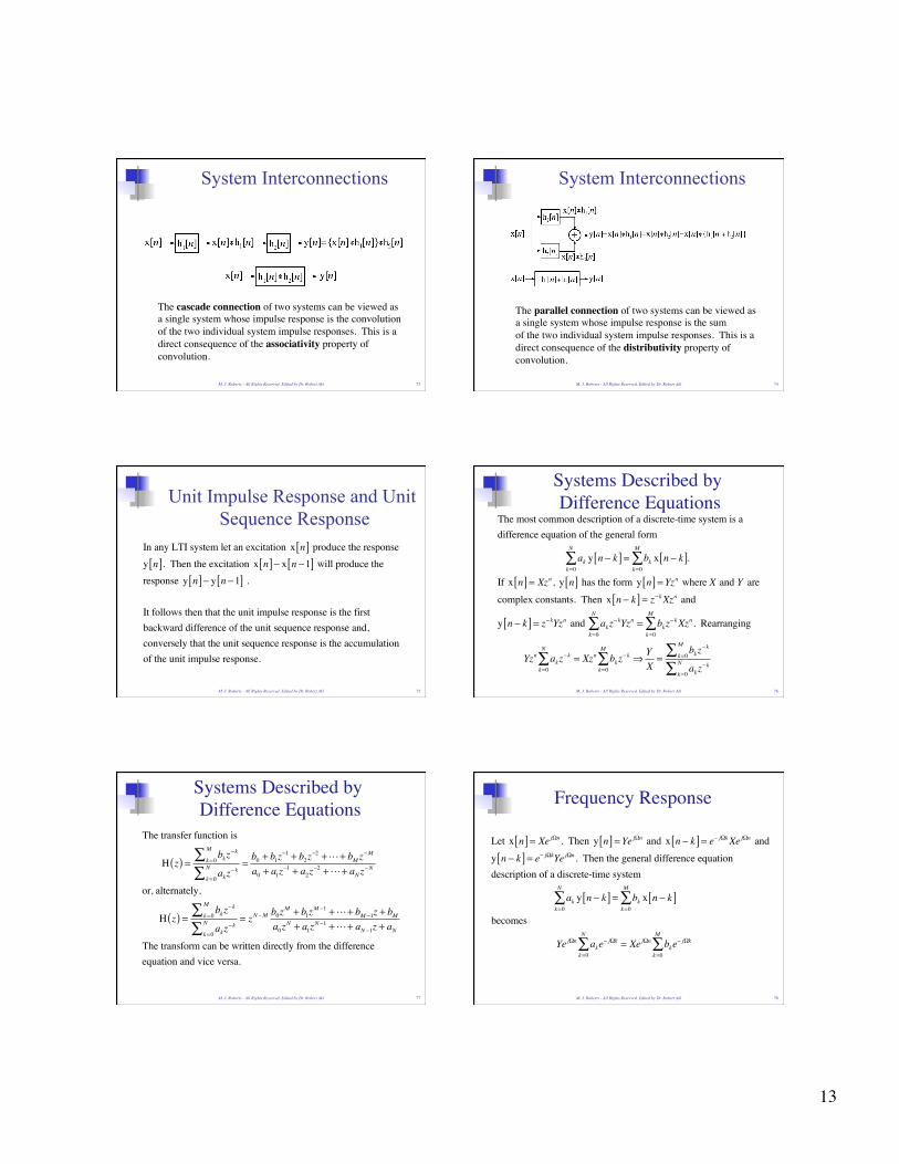
System Interconnections
The cascade connection of two systems can be viewed as a single system whose impulse response is the convolution of the two individual system impulse responses. This is a direct consequence of the associativity property of convolution.
M. J. Roberts - All Rights Reserved. Edited by Dr. Robert Akl 73
System Interconnections
The parallel connection of two systems can be viewed as a single system whose impulse response is the sum of the two individual system impulse responses. This is a direct consequence of the distributivity property of convolution.
M. J. Roberts - All Rights Reserved. Edited by Dr. Robert Akl 74
Unit Impulse Response and Unit Sequence Response
In any LTI system let an excitation x n[ ] produce the response y n[ ]. Then the excitation x n[ ]− x n −1[ ] will produce the response y n[ ]− y n −1[ ] .
It follows then that the unit impulse response is the first backward difference of the unit sequence response and, conversely that the unit sequence response is the accumulationof the unit impulse response.
M. J. Roberts - All Rights Reserved. Edited by Dr. Robert Akl 75
The most common description of a discrete-time system is adifference equation of the general form
ak y n − k[ ]k=0
N
∑ = bk x n − k[ ]k=0
M
∑ .
If x n[ ] = Xzn , y n[ ] has the form y n[ ] = Yzn where X and Y are
complex constants. Then x n − k[ ] = z−k Xzn and
y n − k[ ] = z−kYzn and akz−kYzn
k=0
N
∑ = bkz−k Xzn
k=0
M
∑ . Rearranging
Yzn akz−k
k=0
N
∑ = Xzn bkz−k
k=0
M
∑ ⇒ YX=
bkz−k
k=0
M∑akz
−kk=0
N∑
Systems Described by Difference Equations
M. J. Roberts - All Rights Reserved. Edited by Dr. Robert Akl 76
The transfer function is
H z( ) =bkz
−kk=0
M∑akz
−kk=0
N∑=b0 + b1z
−1 + b2z−2 ++ bM z
−M
a0 + a1z−1 + a2z
−2 ++ aNz−N
or, alternately,
H z( ) =bkz
−kk=0
M∑akz
−kk=0
N∑= zN −M b0z
M + b1zM −1 ++ bM −1z + bM
a0zN + a1z
N −1 ++ aN −1z + aNThe transform can be written directly from the difference equation and vice versa.
Systems Described by Difference Equations
M. J. Roberts - All Rights Reserved. Edited by Dr. Robert Akl 77
Frequency Response
Let x n[ ] = XejΩn . Then y n[ ] = Ye jΩn and x n − k[ ] = e− jΩk Xe jΩn and
y n − k[ ] = e− jΩkYe jΩn . Then the general difference equation description of a discrete-time system
ak y n − k[ ]k=0
N
∑ = bk x n − k[ ]k=0
M
∑becomes
Ye jΩn ake− jΩk
k=0
N
∑ = XejΩn bke− jΩk
k=0
M
∑
M. J. Roberts - All Rights Reserved. Edited by Dr. Robert Akl 78

14
Frequency Response
M. J. Roberts - All Rights Reserved. Edited by Dr. Robert Akl 79
Frequency Response Example
M. J. Roberts - All Rights Reserved. Edited by Dr. Robert Akl 80
Frequency Response Example
M. J. Roberts - All Rights Reserved. Edited by Dr. Robert Akl 81