TIME ASYMMETRY IN NONEQUILIBRIUM STATISTICAL MECHANICS

TIME ASYMMETRY INNONEQUILIBRIUM STATISTICAL MECHANICS

Pierre GASPARDBrussels, Belgium

J. R. Dorfman, College Park S. Ciliberto, LyonT. Gilbert, Brussels N. Garnier, LyonD. Andrieux, Brussels S. Joubaud, Lyon A. Petrosyan, Lyon

• INTRODUCTION: THE BREAKING OF TIME-REVERSAL SYMMETRY• FLUCTUATION THEOREMS FOR CURRENTS & NONLINEAR RESPONSE• ENTROPY PRODUCTION &

TIME ASYMMETRY OF NONEQUILIBRIUM FLUCTUATIONS• CONCLUSIONS

BREAKING OF TIME-REVERSAL SYMMETRY Θ(r,v) = (r,−v)

Newton’s equation of mechanics is time-reversal symmetric if the Hamiltonian H is even in the momenta.

Liouville equation of statistical mechanics, ruling the time evolution of the probability density p is also time-reversal symmetric.

The solution of an equation may have a lower symmetry than the equation itself (spontaneous symmetry breaking).

Typical Newtonian trajectories T are different from their time-reversal image Θ T : Θ T ≠ T

Irreversible behavior is obtained by weighting differently the trajectories T and their time-reversal image Θ T with a probability measure.

Spontaneous symmetry breaking: relaxation modes of an autonomous system

Explicit symmetry breaking: nonequilibrium steady state by the boundary conditions

€

∂p∂t

= H, p{ } = ˆ L p

P. Gaspard, Physica A 369 (2006) 201-246.

STOCHASTIC DESCRIPTIONIN TERMS OF A MASTER EQUATION

€

ddtPt (ω) = Pt (ω') Wρ (ω' |ω) − Pt (ω) W−ρ (ω |ω ')[ ]

ρ ,ω '(≠ω )∑

€

Wρ (ω |ω ')

Liouville’s equation of the Hamiltonian dynamics -> reduced description in terms of the coarse-grained states ω -> master equation for the probability to visit the state ω by the time t : Pt(ω)

rate of the transition

€

ω→ρ

ω'

€

ρ = ±1,...,±r due to the elementary process

A trajectory is a solution of Hamilton’s equations of motion: Γ(t;r0,p0)

Coarse-graining: cell ω in the phase space stroboscopic observation of the trajectory with sampling time Δt : Γ(nΔt;r0,p0) in cell ωn path or history: ω = ω0ω1ω2…ωn−1

-> statistical description of the equilibrium and nonequilibrium fluctuations

= 0 steady state

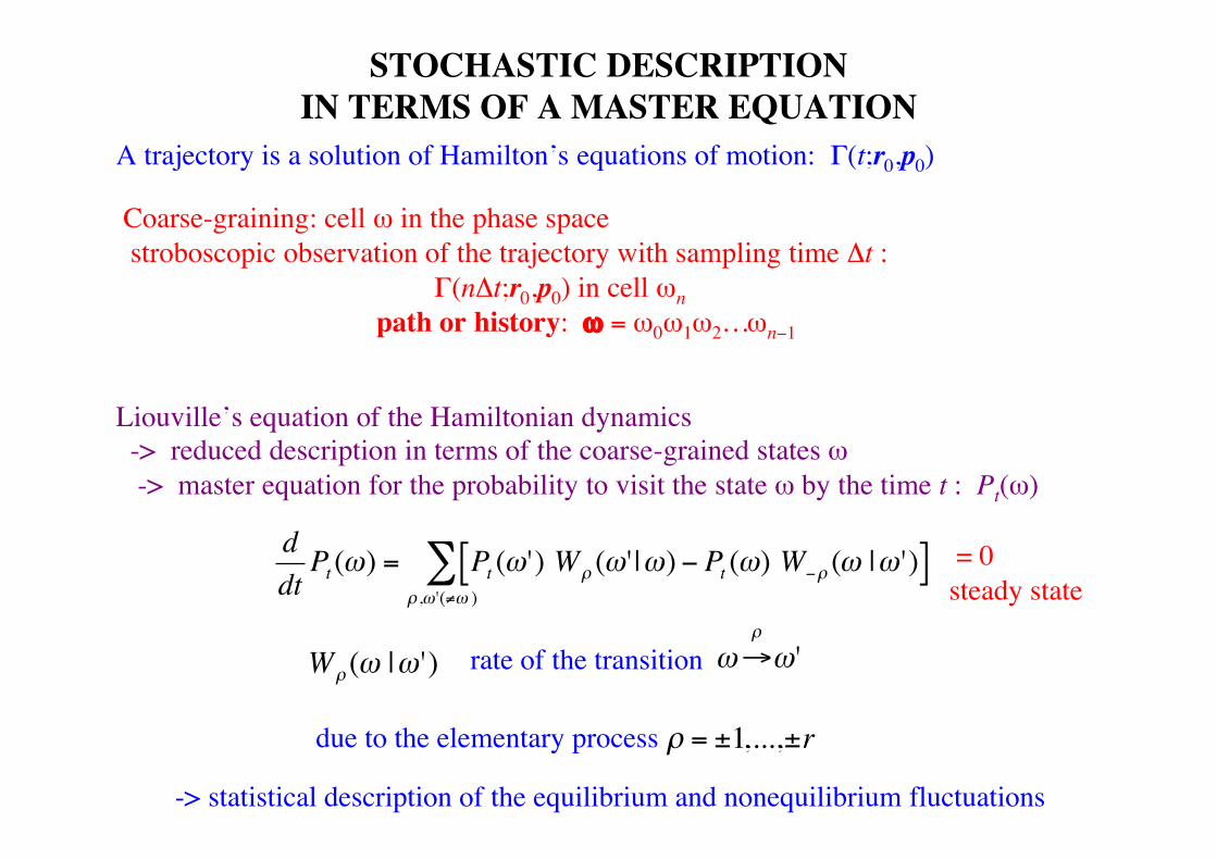
FLUCTUATION THEOREM FOR THE CURRENTS

steady state fluctuation theorem for the currents (2004):

affinities or thermodynamic forces:

fluctuating currents:

thermodynamic entropy production:

€

diSdt st

= Aγ Jγγ =1

c

∑ ≥ 0

€

Jγ =1t

jγ (t ')0

t

∫ dt '

€

Aγ =ΔGγ

T=Gγ −Gγ

eq

T

€

P Jγ =αγ{ }P Jγ = −αγ{ }

≈ etkB

Aγαγγ

∑

-> Onsager reciprocity relations and their generalizations to nonlinear response

D. Andrieux & P. Gaspard, J. Chem. Phys. 121 (2004) 6167; J. Stat. Phys. 127 (2007) 107.

ex: • electric currents in a nanoscopic conductor • rates of chemical reactions • velocity of a linear molecular motor • rotation rate of a rotary molecular motor

€

t→ +∞

Schnakenberg network theory (Rev. Mod. Phys. 1976): cycles in the graph of the process

BEYOND LINEAR RESPONSE & ONSAGER RECIPROCITY RELATIONS

€

q( λγ ,Aγ{ }) = limt→∞

−1tln exp − λγ jγ t '( )dt '

0

t

∫γ

∑

noneq.

€

Jα =∂q∂λα λα = 0

= LαβAββ

∑ + MαβγAβAγβ ,γ∑ + Nαβγδ AβAγ

β ,γ ,δ∑ Aδ +L

€

Mαβγ = 12 Rαβ ,γ + Rαγ ,β( )

€

Lαβ = Lβα is totally symmetric

€

Rαβ ,γ = −∂ 3q

∂λα∂λβ∂Aγ(0;0)

average current:

fluctuation theorem for the currents:

Onsager reciprocity relations:

relations for nonlinear response:

higher-order nonequilibrium coefficients:

generating function of the currents:

linear response coefficients:

€

Lαβ = −12

∂ 2q∂λα∂λβ

(0;0) =12

jα (t) − jα[ ] jβ (0) − jβ[ ]−∞

+∞

∫ dt

(Schnakenberg network theory)

D. Andrieux & P. Gaspard, J. Chem. Phys. 121 (2004) 6167; J. Stat. Mech. (2007) P02006.

linear response coefficients: (Green-Kubo formulas)

€

q( λγ ,Aγ{ }) = q( Aγ − λγ ,Aγ{ })

€

Microreversibility: Hamilton’s equations are time-reversal symmetric. If Γ(t;r0,p0) is a solution of Hamilton’s equation, then Γ(−t;r0,−p0) is also a solution. But, typically, Γ(t;r0,p0) ≠ Γ(−t;r0,−p0).

Coarse-graining: cell ω in the phase space stroboscopic observation of the trajectory with sampling time Δt : Γ(nΔt;r0,p0) in cell ωn path or history: ω = ω0ω1ω2…ωn−1

If ω = ω0ω1ω2…ωn−1 is a possible path, then ωR = ωn−1…ω2ω1ω0 is also a possible path. But, again, ω ≠ ωR.

Statistical description: probability of a path or history: equilibrium steady state: Peq(ω0ω1ω2…ωn−1) = Peq(ωn−1…ω2ω1ω0) nonequilibrium steady state: Pneq(ω0ω1ω2…ωn−1) ≠ Pneq(ωn−1…ω2ω1ω0)

In a nonequilibrium steady state, ω and ωR have different probability weights. Explicit breaking of the time-reversal symmetry by the nonequilibrium boundary conditions

FLUCTUATIONS AND MICROREVERSIBILITY

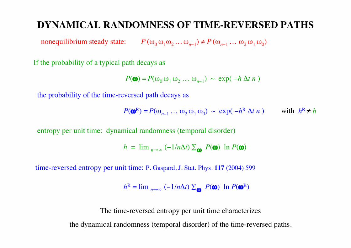
DYNAMICAL RANDOMNESS OF TIME-REVERSED PATHS

€

nonequilibrium steady state: P (ω0 ω1ω2 … ωn−1) ≠ P (ωn−1 … ω2 ω1 ω0)

If the probability of a typical path decays as

P(ω) = P(ω0 ω1 ω2 … ωn−1) ~ exp( −h Δt n )

the probability of the time-reversed path decays as

P(ωR) = P(ωn−1 … ω2 ω1 ω0) ~ exp( −hR Δt n ) with hR ≠ h

entropy per unit time: dynamical randomness (temporal disorder)

h = lim n→∞ (−1/nΔt) ∑ω P(ω) ln P(ω)

time-reversed entropy per unit time: P. Gaspard, J. Stat. Phys. 117 (2004) 599

hR = lim n→∞ (−1/nΔt) ∑ω P(ω) ln P(ωR)

The time-reversed entropy per unit time characterizes

the dynamical randomness (temporal disorder) of the time-reversed paths.

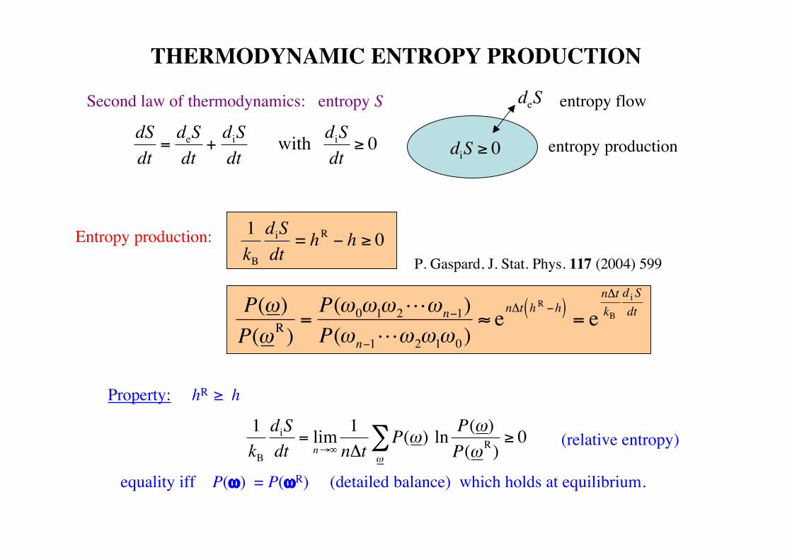
THERMODYNAMIC ENTROPY PRODUCTION

€

Property: hR ≥ h

(relative entropy)

equality iff P(ω) = P(ωR) (detailed balance) which holds at equilibrium.

Second law of thermodynamics: entropy S

€

dSdt

=deSdt

+diSdt

with diSdt

≥ 0

€

deS

€

diS ≥ 0

Entropy production:

€

1kBdiSdt= hR − h ≥ 0

P. Gaspard, J. Stat. Phys. 117 (2004) 599

€

P(ω)P(ωR )

=P(ω0ω1ω2Lωn−1)P(ωn−1Lω2ω1ω0)

≈ enΔt hR −h( ) = e

nΔtkB

d i Sdt

€

1kB

diSdt

= limn→∞

1nΔt

P(ω)ω

∑ ln P(ω)P(ωR)

≥ 0

entropy flow

entropy production

PROOF FOR CONTINUOUS-TIME JUMP PROCESSES

Pauli-type master equation:

nonequilibrium steady state:

τ-entropy per unit time: P. Gaspard & X.-J. Wang, Phys. Reports 235 (1993) 291

time-reversed τ-entropy per unit time: P. Gaspard, J. Stat. Phys. 117 (2004) 599


€

ddtpt (ω ') = pt (ω)Wωω ' − pt (ω ')Wω 'ω[ ]

ω

∑

€

ddtp(ω ') = 0

€

h(τ ) = ln eτ

p(ω)Wωω 'ω≠ω '∑ − p(ω)Wωω '

ω≠ω '∑ lnWωω ' +O(τ )

€

hR(τ ) = ln eτ

p(ω)Wωω 'ω≠ω '∑ − p(ω)Wωω '

ω≠ω '∑ lnWω 'ω +O(τ )

€

hR(τ ) − h(τ ) =12

p(ω)Wωω ' − p(ω ')Wω 'ω[ ]ω≠ω '∑ ln p(ω)Wωω '

p(ω ')Wω 'ω

+O(τ) ≈ 1kB

diSdt

(τ → 0)

Luo Jiu-li, C. Van den Broeck, and G. Nicolis, Z. Phys. B- Cond. Mat. 56 (1984) 165J. Schnakenberg, Rev. Mod. Phys. 48 (1976) 571

PROOF FOR THERMOSTATED DYNAMICAL SYSTEMS

entropy per unit time:

time-reversed entropy per unit time:


δ is the diameter of the phase-space cells

T. Gilbert, P. Gaspard, and J. R. Dorfman (2007)

€

limδ →0

h = λ jλ j >0∑ = hKS

€

limδ →0

(hR − h) = − λ jj∑ =

1kB

diSdt€

limδ →0

hR = − λ jλ j <0∑

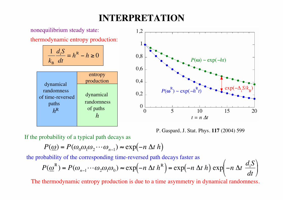
INTERPRETATION

€

nonequilibrium steady state: thermodynamic entropy production:

€


€

P(ω) = P(ω0ω1ω2Lωn−1) ≈ exp −n Δt h( )

€

P(ωR ) = P(ωn−1Lω2ω1ω0) ≈ exp −n Δt hR( ) = exp −n Δt h( ) exp −n Δt diSdt

If the probability of a typical path decays as

the probability of the corresponding time-reversed path decays faster as

The thermodynamic entropy production is due to a time asymmetry in dynamical randomness.

entropy production dynamical

randomnessof time-reversed paths hR

dynamical randomness of paths h

P. Gaspard, J. Stat. Phys. 117 (2004) 599

relaxation time:

€

τR =α /k = 3.05 10−3s

DRIVEN BROWNIAN MOTION

trap stiffness:

€

k = 9.62 10−6 kg s−2

trap velocity:

€

u = ± 4.24 µm/s

Polystyrene particle of 2 µm diameter in a 20% glycerol-water solution at temperature 298 K, driven by an optical tweezer.

D. Andrieux, P. Gaspard, S. Ciliberto, N. Garnier, S. Joubaud, and A. Petrosyan, Phys. Rev. Lett. 98 (2007) 150601

Langevin equation:

€

dxdt

= −x − utτR

+2kBTα

ξ t

dissipated heat:

€

Qt = −k ˙ x t ' (xt ' − ut ') dt'0

t

∫

€

Qt =α u2t

driving force:

€

F = −k(x − ut)

€

position x

€

friction α

€

white noise ξ t

mean dissipated heat:

€

relative position z = x − ut

u < 0

u > 0

comoving frame of reference:

€

dzdt

= −zτR

− u +2αβ

ξ t

€

z ≡ x − ut

€

pst (z) =βk2πexp −βk

2(z + uτR )

2

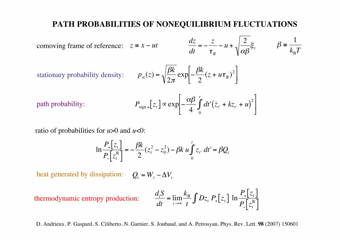
PATH PROBABILITIES OF NONEQUILIBRIUM FLUCTUATIONS


stationary probability density:

path probability:

€

Psign u zt[ ]∝exp −αβ4

dt ' ˙ z t ' + kzt ' + u( )2

0

t

∫

€

ln P+ zt[ ]P− zt

R[ ]= −

βk2

(zt2 − z0

2) −βk u zt ' dt '0

t

∫ = βQt

ratio of probabilities for u>0 and u<0:

€

diSdt

= limt→∞

kB

tDzt P+∫ zt[ ] ln

P+ zt[ ]P− zt

R[ ]


€

β ≡1kBT

€

Qt =Wt −ΔVt heat generated by dissipation:

path:

€

Zm = z(mτ),...,z(mτ + nτ − τ )[ ]

€

H(ε,τ,n) = −1M

lnP+ Zm[ ]m=1

M

∑

RELATIONSHIP TO DYNAMICAL RANDOMNESS


(ε,τ)-entropy per unit time:

path probability:

€

diSdt

= kB limε ,τ→∞hR(ε,τ ) − h(ε,τ )[ ]

€

P+ Zm[ ] = P z(mτ) − z( jτ) < ε,..., z(mτ + nτ − τ ) − z( jτ + nτ − τ ) < ε[ ]

€

HR(ε,τ,n) = −1M

lnP− ZmR[ ]

m=1

M

∑

€

h(ε,τ ) = limn→∞

1τH(ε,τ,n +1) −H(ε,τ,n)[ ]

€

hR(ε,τ ) = limn→∞

1τHR (ε,τ,n +1) −HR (ε,τ,n)[ ]time-reversed (ε,τ)-entropy per unit time:

time-reversed (ε,τ)-entropy:

(ε,τ)-entropy:


algorithm of time series analysis by Grassberger & Procaccia (1980’s)

DRIVEN BROWNIAN MOTION

thermodynamic entropy production:€

ε = k 0.558 nm k =1- 20

sampling frequency: 8192 Hz

resolution:

(ε,τ)-entropy

time-reversed (ε,τ)-entropy

time series:

€

2 107

€

diSdt

=1Td Qt

dt=α u2

T


€

diSdt

= kB limε ,τ→∞hR(ε,τ ) − h(ε,τ )[ ]

DRIVEN BROWNIAN PARTICLE

€

ε = k 0.558 nm k =11- 20 resolution:

dissipated heat along the random path zt

potentiel velocity:

€

u = ± 4.24 µm/s

€

ln P+ zt[ ]P− zt

R[ ]= βQt

ratio of probabilities for u>0 and u<0:

D. Andrieux, P. Gaspard, S. Ciliberto, N. Garnier, S. Joubaud,and A. Petrosyan, Phys. Rev. Lett. 98 (2007) 150601

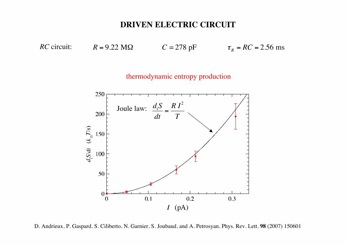
RC circuit:

€

R = 9.22 MΩ C = 278 pF τR = RC = 2.56 ms

DRIVEN ELECTRIC CIRCUIT

thermodynamic entropy production

€

diSdt

=R I 2

TJoule law:


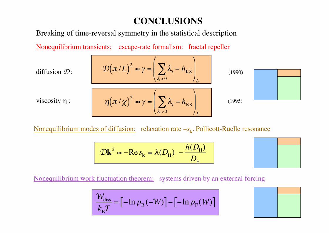
CONCLUSIONSBreaking of time-reversal symmetry in the statistical description

Nonequilibrium work fluctuation theorem: systems driven by an external forcing

€

Wdiss

kBT= −ln pR (−W)[ ] − −ln pF(W)[ ]

€

Dk2 ≈ −Re sk = λ(DH) − h(DH)DH

Nonequilibrium modes of diffusion: relaxation rate −sk, Pollicott-Ruelle resonance

€

D π /L( )2 ≈ γ = λiλi >0∑ − hKS

L

Nonequilibrium transients: escape-rate formalism: fractal repeller

diffusion D : (1990)

viscosity η : (1995)

€

η π /χ( )2 ≈ γ = λiλi >0∑ − hKS

L

CONCLUSIONS (cont’d)

thermodynamic entropy production = temporal disorder of time-reversed paths hR − temporal disorder of paths h= time asymmetry in dynamical randomness

Theorem of nonequilibrium temporal ordering as a corollary of the second law:In nonequilibrium steady states, the typical paths are more ordered in time than thecorresponding time-reversed paths.Boltzmann’s interpretation of the second law:Out of equilibrium, the spatial disorder increases in time.

€


Nonequilibrium steady states:

Explicit breaking of time-reversal symmetry by the nonequilibrium conditions.

Fluctuation theorem for the currents:

€

1kB

Aγαγγ∑ = −lim

t→∞

1tlnP Jγ = −αγ{ }

− −lim

t→∞

1tlnP Jγ =αγ{ }

Entropy production and temporal disorder:

Toward a statistical thermodynamics for out-of-equilibrium nanosystems

http://homepages.ulb.ac.be/~gaspard

Documents

TIME ASYMMETRY IN NONEQUILIBRIUM STATISTICAL MECHANICS