MICROREVERSIBILITY AND TIME ASYMMETRY INNONEQUILIBRIUM STATISTICAL MECHANICS AND

THERMODYNAMICSPierre GASPARD

Université Libre de Bruxelles, Brussels, Belgium

David ANDRIEUX, Brussels & YaleMassimiliano ESPOSITO, BrusselsTakaaki MONNAI, TokyoShuichi TASAKI, Tokyo

• INTRODUCTION: TIME-REVERSAL SYMMETRY BREAKING• FLUCTUATION THEOREM FOR CURRENTS & NONLINEAR RESPONSE• THEOREM OF NONEQUILIBRIUM TEMPORAL ORDERING• CONCLUSIONS

ICTS Program on Non-Equilibrium Statistical Physics,Indian Institute of Technology, Kanpur

NESP2010 Ilya Prigogine Lecture, 30 January 2010

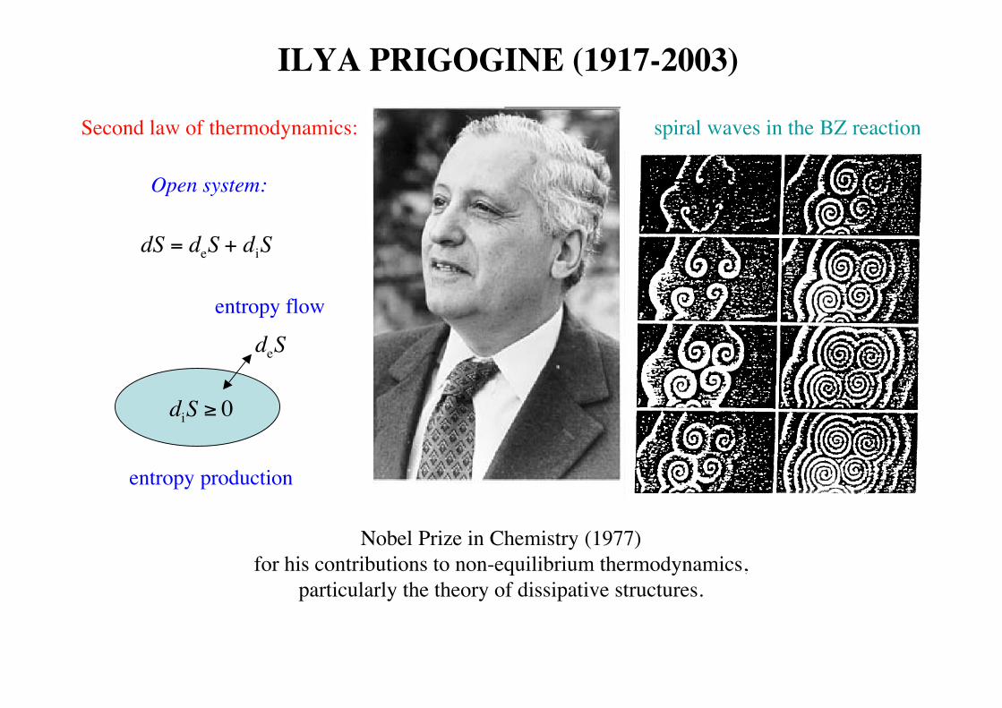
Nobel Prize in Chemistry (1977)for his contributions to non-equilibrium thermodynamics,

particularly the theory of dissipative structures.

Second law of thermodynamics:

€

dS = deS + diS

€

deS

€

diS ≥ 0

entropy flow

entropy production

Open system:

spiral waves in the BZ reaction

ILYA PRIGOGINE (1917-2003)

THE SCALE OF THINGS: NANOMETERS AND MORE

Publication of the US Government

F1-ATPase NANOMOTORH. Noji, R. Yasuda, M. Yoshida, & K. Kinosita Jr., Nature 386 (1997) 299

R. Yasuda, H. Noji, M. Yoshida, K. Kinosita Jr. & H. Itoh, Nature 410 (2001) 898

power = 10−18 Watt

chemical fuel of the F1 nanomotor: ATP adenosine triphosphate

F1 = (αβ)3γ protein:

(Courtesy Professor K. Kinosita Jr.)

OUT-OF-EQUILIBRIUM NANOSYSTEMS

Examples: - electronic nanocircuits- heterogeneous catalysis at the nanoscale- molecular motors- ribosome- RNA polymerase: information processing

Structure in 3D space:

• no flux

• no entropy production

• no energy supply needed

• equilibrium

• in contact with one reservoir

Nanosystems sustaining fluxes of matter or energy, dissipating energy supply

€

Jγ = 0

€

diSdt= 0

Dynamics in 4D space-time:

• flux

• entropy production

• energy supply required

• nonequilibrium

• in contact with several reservoirs

€

Jγ ≠ 0

€

diSdt

> 0

MICRODYNAMICS: TIME-REVERSAL SYMMETRY Θ(r,v) = (r,−v)

Newton’s equation of mechanics is time-reversal symmetric.

velocity v

position r

Phase space:

0

trajectory 1 = Θ (trajectory 2)

time reversal Θ

trajectory 2 = Θ (trajectory 1)

€

m d2rdt 2

= F(r)

BREAKING OF TIME-REVERSAL SYMMETRY

Selecting the initial condition typically breaks the time-reversal symmetry.

velocity v

position r

Phase space:

0

This trajectory is selected by the initial condition.

time reversal Θ

The time-reversed trajectory is not selected by the initial condition if it is distinct from the selected trajectory.

initial condition* €

m d2rdt 2

= F(r)

HARMONIC OSCILLATOR

All the trajectories are time-reversal symmetric in the harmonic oscillator.

velocity v

position r

Phase space:

0 time reversal Θ

self-reversed trajectories

€

m d2rdt 2

= −kr

FREE PARTICLE

Almost all of the trajectories are distinct from their time reversal.

velocity v

position r

Phase space:

0 time reversal Θ

self-reversed trajectories at zero velocity

€

m d2rdt 2

= 0

Antares

Aldebaran

BREAKING OF TIME-REVERSAL SYMMETRYIN NONEQUILIBRIUM STEADY STATES

weighting each trajectory with a probability

velocity v

0 time reversal Θ

position r

Phase space:

Nonequilibrium stationary probability distribution: directionality

rese

rvoi

r 1 reservoir 2

DETAILED BALANCING AT EQUILIBRIUM

The time-reversal symmetry, e.g. detailed balancing, is restored at equilibrium.

velocity v

0 time reversal Θ

position r

Phase space:

Equilibrium stationary probability distribution: no directionality

BREAKING OF TIME-REVERSAL SYMMETRY Θ(r,v) = (r,−v)

Newton’s equation of mechanics is time-reversal symmetric if the Hamiltonian H is even in the momenta.

Liouville equation of statistical mechanics,ruling the time evolution of the probability density pis also time-reversal symmetric.

The solution of an equation may have a lower symmetry than the equation itself (spontaneous symmetry breaking).

Typical Newtonian trajectories T are different from their time-reversal image Θ T : Θ T ≠ T

Irreversible behavior is obtained by weighting differently the trajectories T and their time-reversal image Θ T with a probability measure.

Stationary probability distribution: (random event A)equilibrium: Peq(Θ A) = Peq(A) (detailed balancing)nonequilibrium: Pneq(Θ A) ≠ Pneq(A)

€

∂p∂t

= H, p{ } = ˆ L p

STEADY-STATE FLUCTUATION THEOREM FOR CURRENTS

De Donder affinities or thermodynamic forces:

fluctuating currents:

thermodynamic entropy production:

€

diSdt st

= Aγ Jγγ =1

c

∑ ≥ 0

€

Jγ =1t

jγ (t ')0

t

∫ dt '

€

Aγ =ΔGγ

T=Gγ −Gγ

eq

T

€

t→ +∞

€

P +Jγ{ }P −Jγ{ }

≈ etkB

Aγ Jγγ

∑

( free energy sources)

D. Andrieux & P. Gaspard, Fluctuation theorem and Onsager reciprocity relations, J. Chem. Phys. 121 (2004) 6167.

D. Andrieux & P. Gaspard, Fluctuation theorem for currents and Schnakenberg network theory, J. Stat. Phys. 127 (2007) 107.

valid far from equilibrium as well as close to equilibrium

ex: • electric currents in a nanoscopic conductor • rates of chemical reactions • velocity of a molecular motor

Stationary probability distribution P :

• No directionality at equilibrium Aγ = 0• Directionality out of equilibrium Aγ ≠ 0

time interval:

GENERATING FUNCTION OF THE CURRENTS:FULL COUNTING STATISTICS

€

Q( λγ ,Aγ{ }) = limt→∞

−1tln exp − λγ jγ t '( )dt '

0

t

∫γ

∑

noneq.

average currents:

fluctuation theorem for the currents bis:

generating function:

€

Q( λγ ,Aγ{ }) =Q( Aγ − λγ ,Aγ{ })

€

P +Jγ{ }P −Jγ{ }

≈ etkB

Aγ Jγγ

∑ fluctuation theorem for the currents:

with the probability distribution P

€

Jα =∂Q∂λα λα = 0

= Lα,βAββ

∑ +12

Mα ,βγAβAγβ ,γ∑ +

16

Nα ,βγδ AβAγβ ,γ ,δ∑ Aδ +L

LINEAR & NONLINEAR RESPONSE THEORY

€

Lα,β = Lβ ,α is totally symmetric Onsager reciprocity relations:

€

Lα,β = −12

∂ 2Q∂λα∂λβ

0,0{ }( ) =12

jα (t) − jα[ ] jβ (0) − jβ[ ]−∞

+∞

∫ dt

Green-Kubo formulas: 2nd cumulants

2nd responses of currents:

€

Mα,βγ ≡∂ 3Q

∂λα∂Aβ∂Aγ0,0{ }( )

2nd responses of currents =1st responses of 2nd cumulants:

D. Andrieux & P. Gaspard, J. Chem. Phys. 121 (2004) 6167; J. Stat. Mech. (2006) P01011.

1st responses of 2nd cumulants:

€

Rαβ ,γ ≡ −∂ 3Q

∂λα∂λβ∂Aγ0,0{ }( )

€

Mα,βγ = 12 Rαβ ,γ + Rαγ ,β( )

€

Rαβ ,γ =∂∂Aγ

jα (t) − jα[ ] jβ (0) − jβ[ ]noneq.

−∞

+∞

∫ dtA= 0

nonlinear response coefficients at 2nd order

linear response coefficients

= 1st responses of diffusivities:

NONLINEAR RESPONSE THEORY (cont’d)

€

Jα =∂Q∂λα λα = 0

= Lα,βAββ

∑ +12

Mα ,βγAβAγβ ,γ∑ +

16

Nα ,βγδ AβAγβ ,γ ,δ∑ Aδ +Laverage current:

fluctuation theorem for the currents:

3rd responses of currents:

€

Q( λγ ,Aγ{ }) =Q( Aγ − λγ ,Aγ{ })

€

Nα,βγδ ≡∂ 4Q

∂λα∂Aβ∂Aγ∂Aδ0,0{ }( )

relations at 3nd order:

D. Andrieux & P. Gaspard, J. Stat. Mech. (2007) P02006.

2nd responses of 2nd cumulants:

€

Tαβ ,γδ ≡ −∂ 4Q

∂λα∂λβ∂Aγ∂Aδ0,0{ }( )

€

Nα,βγδ = 12 Tαβ ,γδ + Tαγ ,βδ + Tαδ ,βγ − Sαβγ ,δ( )

nonlinear response coefficients at 3rd order

1st responses of 3rd cumulants = 4th cumulants:

€

Sαβγ ,δ ≡∂ 4Q

∂λα∂λβ∂λγ∂Aδ0,0{ }( ) = −

12

∂ 4Q∂λα∂λβ∂λγ∂λδ

0,0{ }( )

QUANTUM NANOSYSTEMS de Broglie quantum wavelength: λ = h/(mv)

electrons are much lighter than nuclei -> quantum effects are important in electronics

current fluctuations in a GaAs-GaAlAs quantum dot (QD): real-time detection with a quantum point contact (QPC)

S. Gustavsson et al., Counting Statistics of Single Electron Transport in a Quantum Dot,Phys. Rev. Lett. 96, 076605 (2006).

bidirectionality not observedlimit of a large bias voltage:

€

±eV /2 −ε >> kBT

T = 350 mK

€

VQD =1.2 mV

€

VQPC = 0.5 mV

€

IQD =127 aA

€

IQPC = 4.5 nA

current fluctuations in a AlGaAs/GaAs double quantum dot: real-time detection with a quantum point contact

T. Fujisawa et al., Bidirectional Counting of Single Electrons, Science 312, 1634 (2006).

bidirectionality observed

FULL COUNTING STATISTICS OF FERMIONS• L. S. Levitov & G. B. Lesovik, Charge distribution in quantum shot noise, JETP Lett. 58, 230 (1993)• D. A. Bagrets and Yu. V. Nazarov, Full counting statisticsof charge transfer in Coulomb blockade

systems, Phys. Rev. B 67, 085316 (2003).• J. Tobiska & Yu. V. Nazarov, Inelastic interaction corrections and universal relations for full

counting statistics in a quantum contact, Phys. Rev. B 72, 235328 (2005).• D. Andrieux & P. Gaspard, Fluctuation theorem for transport in mesoscopic systems, J. Stat. Mech.

P01011 (2006).• U. Harbola, M. Esposito, and S. Mukamel, Quantum master equation for electron transport through

quantum dots and single molecules, Phys. Rev. B 74, 235309 (2006).• M. Esposito, U. Harbola, and S. Mukamel, Nonequilibrium fluctuations, fluctuation theorems, and

counting statistics in quantum systems, Rev. Mod. Phys. 81, 1665 (2009).

εµL

µR = µL− eV

€

αρ =Wρ 01( ) = Γρ fρβρ =Wρ 10( ) = Γρ 1− fρ( )

€

ρ = L,R

charging rate from side ρ:

discharging rate from side ρ:

Fermi-Dirac distributions:

€

fρ =1

1+ e(ε−µρ ) /(kBT )

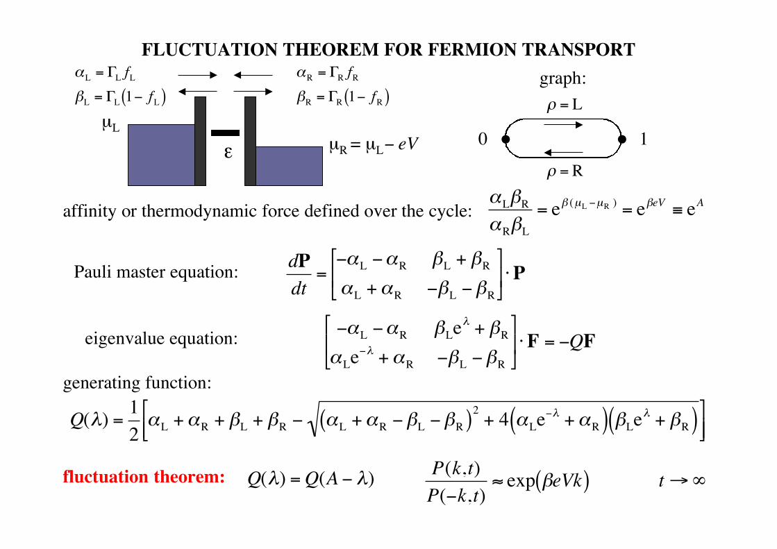
FLUCTUATION THEOREM FOR FERMION TRANSPORT

εµL

µR = µL− eV€

αL = ΓL fLβL = ΓL 1− fL( )

Pauli master equation:

€

dPdt

=−αL −αR βL + βRαL +αR −βL −βR

⋅P

eigenvalue equation:

€

−αL −αR βLeλ + βR

αLe−λ +αR −βL −βR

⋅F = −QF

graph:

0 • • 1

€

ρ = L

€

ρ = R

affinity or thermodynamic force defined over the cycle:

€

αLβRαRβL

= eβ (µL −µR ) = eβeV ≡ eA

€

Q(λ) =12αL +αR + βL + βR − αL +αR −βL −βR( )2 + 4 αLe

−λ +αR( ) βLeλ + βR( )

fluctuation theorem:

€

Q(λ) =Q(A − λ)

€

P(k,t)P(−k,t)

≈ exp βeVk( ) t→∞

€

αR = ΓR fRβR = ΓR 1− fR( )

generating function:

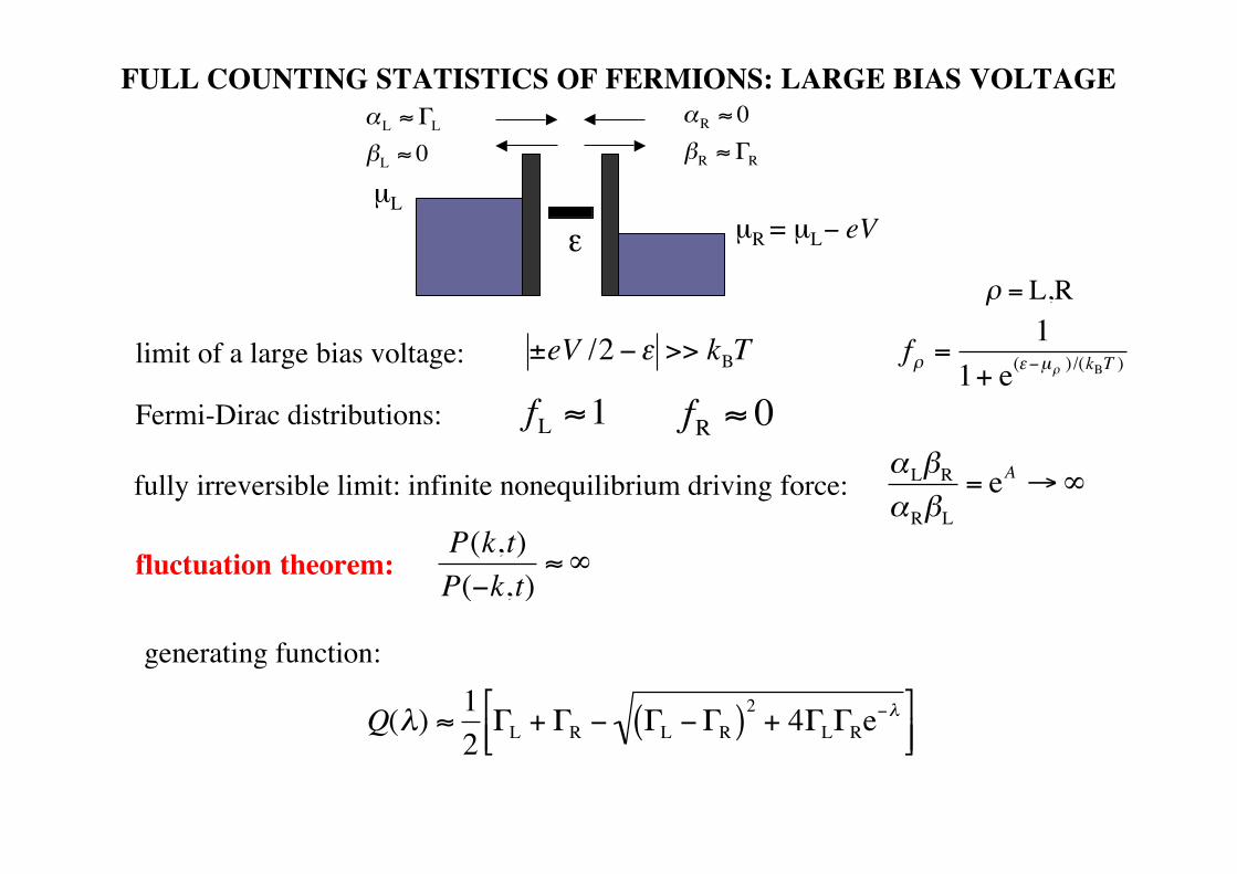
FULL COUNTING STATISTICS OF FERMIONS: LARGE BIAS VOLTAGE

εµL

µR = µL− eV€

αL ≈ ΓLβL ≈ 0

limit of a large bias voltage:

€

αLβRαRβL

= eA →∞

€

Q(λ) ≈ 12ΓL + ΓR − ΓL −ΓR( )2 + 4ΓLΓRe

−λ

fluctuation theorem:

€

P(k,t)P(−k,t)

≈ ∞

€

αR ≈ 0βR ≈ ΓR

generating function:

€

±eV /2 −ε >> kBT

Fermi-Dirac distributions:

€

fL ≈1

€

fR ≈ 0

fully irreversible limit: infinite nonequilibrium driving force:€

fρ =1

1+ e(ε−µρ ) /(kBT )

€

ρ = L,R

QUANTUM FLUCTUATION THEOREM WITH A MAGNETIC FIELD BD. Andrieux, P. Gaspard, T. Monnai & S. Tasaki, The fluctuation theorem for currents in open quantum systems,New J. Phys. 11 (2009) 043014; Erratum 109802

quantum steady-state fluctuation theorem for currents:

affinities or thermodynamic forces:

€

A0 ≡ β1 −β2

Aα ≡ −β1µ1α + β2µ2α for α =1,2,...,c

€

Q λγ ,Aγ{ };B( ) =Q Aγ − λγ ,λγ{ };−B( )

€

Lα,β (B) = Lβ ,α (−B) Casimir-Onsager reciprocity relations:

€

∂ 3Q∂λα∂Aβ∂Aγ

0,0;B( ) = −∂ 3Q

∂λα∂Aβ∂Aγ0,0;−B( )

Rαβ ,γ (B) = Rαβ ,γ (−B) +∂ 3Q

∂λα∂Aβ∂Aγ0,0;B( )

Mα,βγ (B) + Mα ,βγ (−B) = Rαβ ,γ (−B) + Rαγ ,β (−B) +∂ 3Q

∂λα∂Aβ∂Aγ0,0;B( )

linear response coefficients

nonlinear response coefficients: magnetic-field asymmetry

FLUCTUATION THEOREM FOR BOSON TRANSPORT

A single oscillator mode between two heat baths at different temperatures

€

dP(N,t)dt

= βL + βR( ) N +1( )P(N +1,t) − βL + βR( )NP(N,t)

+ αL +αR( )NP(N −1,t) − αL +αR( ) N +1( )P(N,t)eigenvalue equation:

fluctuation theorem:

€

P(k,t)P(−k,t)

≈ exp −hω0 βL −βR( )k[ ] t→∞

• U. Harbola, M. Esposito, and S. Mukamel., Statistics and fluctuation theorem for boson and fermiontransport through mesoscopic junctions, Phys. Rev. B 76, 085408 (2007).

• M. Esposito, U. Harbola, and S. Mukamel., Nonequilibrium fluctuations, fluctuation theorems, andcounting statistics in quantum systems, Rev. Mod. Phys. 81, 1665 (2009).

master equation:

Bose-Einstein distributions:

€

fρ =1

eβρ hω0 −1βL βR

€

αL = ΓL fLβL = ΓL 1+ fL( )

€

αR = ΓR fRβR = ΓR 1+ fR( )

ω0

€

ρ = L,R

€

−Q(λ)F(N,t) = βLeλ + βR( ) N +1( )F(N +1,t) − βL + βR( )NF(N,t)

+ αL +αR( )NF(N −1,t) − αLe−λ +αR( ) N +1( )F(N,t)

affinity or thermodynamic force:

€

αLβRαRβL

= e−hω0 (βL −βR ) ≡ eA

€

Q(λ) =Q(A − λ)

€

Coarse-graining: cell ω in the phase space stroboscopic observation of the trajectory with sampling time Δt : Γ(nΔt;r0,p0) in cell ωn path or history: ω = ω0ω1ω2…ωn−1

If ω = ω0ω1ω2…ωn−1 is a possible path, then ωR = ωn−1…ω2ω1ω0 is also a possible path. But, again, ω ≠ ωR.

Stationary probability distribution as solution of Liouville equation:

Statistical description: probability of a path or history: equilibrium steady state: Peq(ω0ω1ω2…ωn−1) = Peq(ωn−1…ω2ω1ω0) (detailed balancing) nonequilibrium steady state: Pneq(ω0ω1ω2…ωn−1) ≠ Pneq(ωn−1…ω2ω1ω0)

In a nonequilibrium steady state, ω and ωR have different probability weights: breaking of the time-reversal symmetry by the nonequilibrium probability distribution.

STATISTICS OF PATHS / HISTORIES

€

P(ω0ω1ω2 ...ωn−1) = limt→∞

dΓ p(Γ,t) Iω0∩Φ

−Δt ω1( )...∩Φ− ( n−1)Δt ωn−1( )(Γ)∫

TEMPORAL DISORDER

€

nonequilibrium steady state: P (ω0 ω1ω2 … ωn−1) ≠ P (ωn−1 … ω2 ω1 ω0)

If the probability of a typical path decays as (coin tossing Bernoulli process: h = log 2)

P(ω) = P(ω0 ω1 ω2 … ωn−1) ~ exp( −h Δt n )

the probability of the time-reversed path decays as

P(ωR) = P(ωn−1 … ω2 ω1 ω0) ~ exp( −hR Δt n ) with hR ≠ h

temporal disorder per unit time: (dynamical randomness)

h = lim n→∞ (−1/nΔt) ∑ω P(ω) ln P(ω)

time-reversed temporal disorder per unit time: P. Gaspard, J. Stat. Phys. 117 (2004) 599

hR = lim n→∞ (−1/nΔt) ∑ω P(ω) ln P(ωR)

The time-reversed temporal disorder per unit time characterizes

the dynamical randomness of the time-reversed paths.

THERMODYNAMIC ENTROPY PRODUCTION

€

Second law of thermodynamics: entropy S

€

dSdt

=deSdt

+diSdt

with diSdt

≥ 0 €

deS

€

diS ≥ 0

Entropy production:

€

P(ω)P(ωR )

=P(ω0ω1ω2 ... ωn−1)P(ωn−1... ω2ω1ω0)

≈ enΔt hR −h( ) = e

nΔtkB

d i Sdt

entropy flow

entropy production

thermodynamic entropy production = time asymmetry of temporal disorder

€

1kBdiSdt= hR − h ≥ 0

Open system interacting with its environment:

Time-reversed paths are less probable.

Out-of-equilibrium process

P. Gaspard, J. Stat. Phys. 117 (2004) 599P. Gaspard and G. Nicolis, Phys. Rev. Lett. 65 (1990) 1693

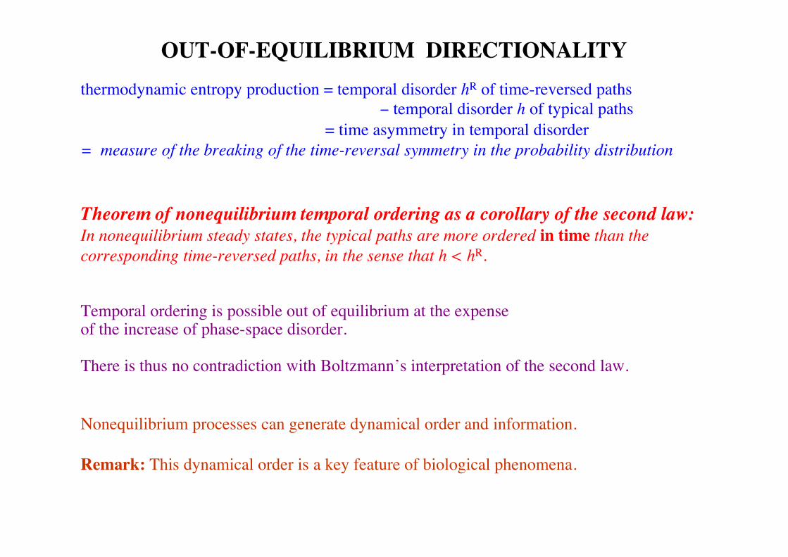
OUT-OF-EQUILIBRIUM DIRECTIONALITY

Theorem of nonequilibrium temporal ordering as a corollary of the second law:In nonequilibrium steady states, the typical paths are more ordered in time than thecorresponding time-reversed paths, in the sense that h < hR.

Temporal ordering is possible out of equilibrium at the expenseof the increase of phase-space disorder.

There is thus no contradiction with Boltzmann’s interpretation of the second law.

Nonequilibrium processes can generate dynamical order and information.

Remark: This dynamical order is a key feature of biological phenomena.

thermodynamic entropy production = temporal disorder hR of time-reversed paths − temporal disorder h of typical paths

= time asymmetry in temporal disorder= measure of the breaking of the time-reversal symmetry in the probability distribution

DEDUCTION OF LANDAUER’S PRINCIPLEErasing information in the memory of a computer is irreversible and dissipates energy.

€

Δ iS = kB hR − h( ) = kBDthermodynamic entropy production per erased bit:

Shannon disorder per bit:

€

D ≡ liml→∞

− 1l

µ(σ1σ 2 ...σ l ) ln µ(σ1σ 2 ...σ l )σ 1σ 2 ...σ l

∑

Landauer’s case of a random binary sequence:

€

Δ iS = kB hR − h( ) = kB ln2

€

01

€

0

D. Andrieux & P. Gaspard, Dynamical randomness, information, and Landauer’s principle,EuroPhysics Letters 81 (2008) 28004

OUT-OF-EQUILIBRIUM FLUCTUATING SYSTEMS

RC electric circuit (Nyquist thermal noise) (Ciliberto et al., 2008)

Brownian particle in an optical trap and a flow(Ciliberto et al., 2008)

Molecular motor F1-ATPase(Kinosita et al., 2001)

laser

Energy supply

R. Yasuda, H. Noji, M. Yoshida, K. Kinosita Jr. & H. Itoh, Nature 410 (2001) 898

D. Andrieux, P. Gaspard, S. Ciliberto, N. Garnier, S. Joubaud, and A. Petrosyan, J. Stat. Mech. (2008) P01002

D. Andrieux, P. Gaspard, S. Ciliberto, N. Garnier, S. Joubaud, and A. Petrosyan, J. Stat. Mech. (2008) P01002

BROWNIAN PARTICLE OUT OF EQUILIBRIUM

particle of 2 µm diameter in an optical trap and a flow of speed ulaser

Temporal disorders of typical and reversed trajectories

Their difference is the thermodynamic production entropy

Irreversibility is observed down to the nanoscale.

probability distributions of positiontrajectories for u and −u

D. Andrieux, P. Gaspard, S. Ciliberto, N. Garnier, S. Joubaud, and A. Petrosyan, J. Stat. Mech. (2008) P01002

€

diSdt

=α u2

T

RC ELECTRIC CIRCUIT OUT OF EQUILIBRIUM

Temporal disorders of typical and reversed trajectories

Their difference is the thermodynamic entropy production.

Irreversibility is observed down to fluctuations of several thousands of electrons.

probability distributions of chargespaths for I and −I

€

R = 9.22 MΩ C = 278 pF τR = RC = 2.56 ms D. Andrieux, P. Gaspard, S. Ciliberto, N. Garnier, S. Joubaud, and A. Petrosyan, J. Stat. Mech. (2008) P01002

€

diSdt

=R I 2

T

Joule law:

OUT-OF-EQUILIBRIUM TRAJECTORIESOF THE MOLECULAR MOTOR

Random trajectories observed in experiments:R. Yasuda, H. Noji, M. Yoshida, K. Kinosita Jr. & H. Itoh, Nature 410 (2001) 898

Random trajectories simulated by a model:P. Gaspard & E. Gerritsma, J. Theor. Biol. 247 (2007) 672

Power of the motor: 10−18 Watt

at equilibrium:…212132131223132… random

out of equilibrium:…123123123123123…regular: directionality

CONCLUSIONS

thermodynamic arrow of time

= time asymmetry in temporal disorder

Theorem of nonequilibrium temporal ordering as a corollary of the second law:Directionality and lowering of randomness in the motion.The farther from equilibrium, the lower the temporal disorder.€

1kBdiSdt= hR − h ≥ 0

Thermodynamic entropy production:

Thermodynamic arrow of time down to the nanoscale

Explanation of directionality in nonequilibrium systems

Breaking of time-reversal symmetry in the statistical description of nonequilibrium systems

Statistical thermodynamics for nonequilibrium nanosystems:• Fluctuation theorem for currents in steady states• Fluctuation theorem for quantum systems• Extensions of Onsager-Casimir reciprocity relations to nonlinear response