Tim Haithcoat University of Missouri Columbia - MSDISmsdis.missouri.edu/resources/intro_to_gis/pdf/Vector.pdf · Tim Haithcoat University of Missouri Columbia With materials from:

12

presented by:

Tim HaithcoatUniversity of Missouri

Columbia

With materials from:

Holly Dickinson, State Universityof New York at Buffalo

Vector GIS

2

Introduction to Vector Data ModelIntroduction to Vector Data Model

• Based on vectors (as opposed to space-occupancy raster structures)

• Fundamental primitive is a point

• Objects are created by connecting pointswith straight lines– Some systems allow points to be connected

using arcs of circles

3

Introduction ContinuedIntroduction Continued

• Areas are defined by sets of lines– The term polygon is synonymous with area in

vector databases because of the use of straight lineconnections between points

• Very large vector databases have been built fordifferent purposes– Vector tends to dominate in transportation, utility,

marketing applications

– Raster & vector both used in resource managementapplications

Example: Vector GIS Data

Example Attributes:city: population, namewells: depthhighway: numberpolitical boundary: typestreams: nameag. land: growth potential, acreageurban land: urban landuse type, acreageairport: name

citywells

ag. landurban landcityhighway airport

highwaypolitical boundarystreams

SCALE

point line area

5

“ARCS”“ARCS”

• When planar enforcement is used, area objects in oneclass or layer cannot overlap and must exhaust thespace of a layer

• Every piece of boundary line is a common boundarybetween two areas

• The stretch of common boundary between twojunctions (nodes) has various names– Edge: favored by graph theorists, “vertex” for the junctions

– Chain: word officially sanctioned by the US NationalStandard

– Arc: used by several systems

6

“ARCS” Continued“ARCS” Continued

• Arcs have attributes which identify thepolygons on either side– these are referred to as “left” and “right” by

reference to the sequence in which the arccoded

• Arcs (chains/edges) are fundamental invector GIS

7

Two Storing AreasTwo Storing Areas

POLYGON STORAGE

• Every polygon is stored as a sequence of coordinates• Although most boundaries are shared between two

adjacent areas, all are input and coded twice, once foreach adjacent polygon

• The two different versions of each internal boundaryline may not coincide

• Difficult to do certain operations (i.e., dissolveboundaries between neighboring areas and merge them

• Used in some current GISs, many automated mappingpackages

8

Two Storing AreasTwo Storing Areas

ARC STORAGE

• Every arc is stored as a sequence of coordinates

• Areas are built by linking arcs

• Only one version of each internal sharedboundary is input and stored

• Used in most current vector-based GISs

9

Database CreationDatabase Creation

• Involves several stages:– Input of the spatial data

– Input of attribute data

– Linking spatial and attribute data

• Spatial data is entered via digitized points andlines, scanned and vectorized lines or directlyfrom other digital sources– Once the spatial data has been entered, much work

is still needed before it can be used

10

Building TopographyBuilding Topography

• Once points are entered and geometric lines arecreated, topology must by “built”– This involves calculating and encoding

relationships between the points, lines and areas

– This info may be automatically coded into tables ofinformation in the database

– Let’s look at an example

Example of “Built” Topology (ARC/INFO)

ArcID

LeftPoly

RtPoly

FromNode

ToNode

1 A 0 c a

2 A B b c

3 C A b a

4 0 C d a

5 C B d b

6 B D e e

7 B 0 d c

Polygon

ID

No. of Arcs List of Arcs

A 3 -1,-2,3

B 4 2,-7,5,0,-6

C 3 -3,-5,4

D 1 6

Node ID

Polygon ID

Arc ID

arc digitized indirection ofarrow

A

e

6

AB

C

e

c

a

d

b

6D

2

3

5

4

0

1

7

12

EditingEditing

• During this topology generation process,problems such as overshoots, undershoots andspikes are either flagged for editing by the useror corrected automatically– Automatic editing involves the use of a tolerance

value which defines the width of a buffer zonearound objects within which adjacent objects shouldbe joined

13

Editing - continuedEditing - continued

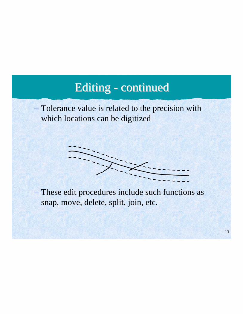
– Tolerance value is related to the precision withwhich locations can be digitized

– These edit procedures include such functions assnap, move, delete, split, join, etc.

14

Relationship between Digitizing & EditingRelationship between Digitizing & Editing

• Digitizing and editing are complementaryactivities– Poor digitizing leads to much need for editing

– Good digitizing can avoid most need for editing

– Both can be very labor-intensive

• The process used to digitize area objects canaffect the need for later editing

15

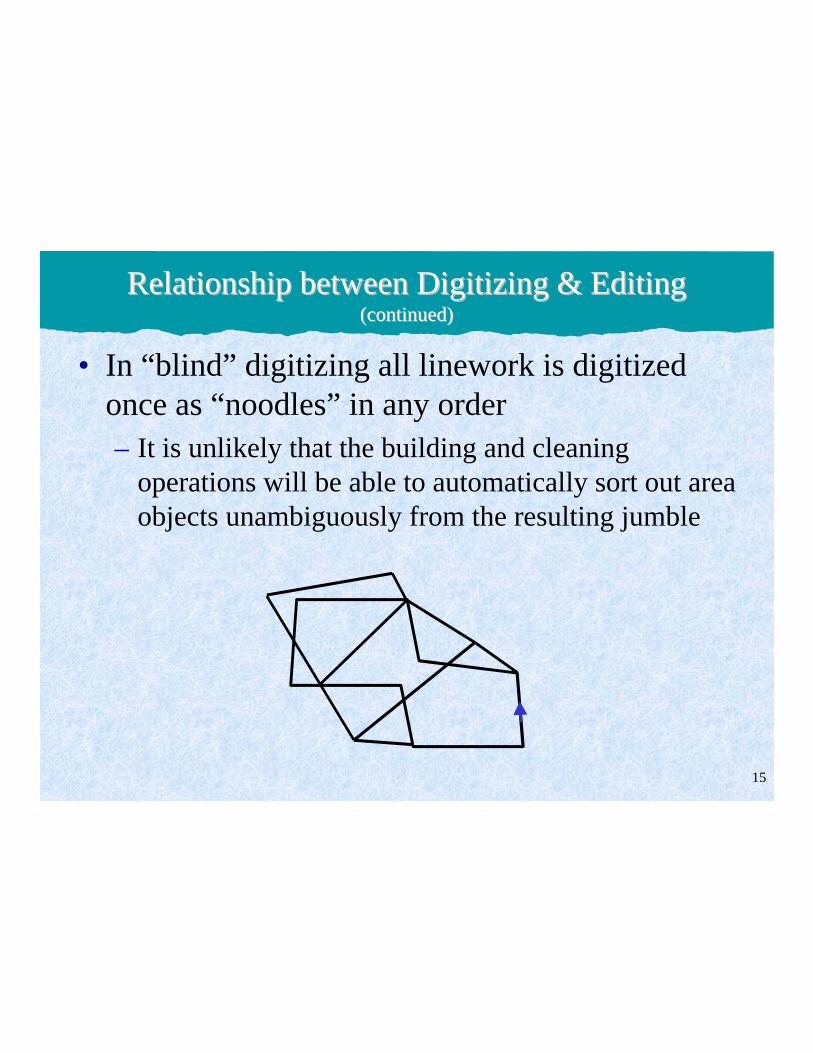
• In “blind” digitizing all linework is digitizedonce as “noodles” in any order– It is unlikely that the building and cleaning

operations will be able to automatically sort out areaobjects unambiguously from the resulting jumble

Relationship between Digitizing & EditingRelationship between Digitizing & Editing(continued)(continued)

16

• Some systems require the user to identifyjunctions between digitized “noodles” explicitly– Usually by touching a special button on the cursor

– Mistakes in building topology are less likely


***

*

17

• Some systems require the user to digitize eachindividual arc/chain separately

– Much easier to sort our polygons - less need forediting


***

*

18

• Some systems support the building of topology“on the fly”– The system searches constantly for complete area

objects as digitizing proceeds

– The users is informed by a sound or by blinking assoon as the object is detected


19

EdgematchingEdgematching

• Compares and adjusts features along the edgesof adjacent map sheets

• Some edgematches merely move objects intoalignment

• Others “join” the pieces together logically -conceptually they become one object– The user “sees” no interruption

• An edgematched database is “seamless” - thesheet edges have disappeared as far as the useris concerned

20

Adding AttributesAdding Attributes

• Once the objects have been formed by buildingtopology, attributes can be keyed in or importedfrom other digital databases

• Once added to the database, attributes must belinked to the different objects– Attributes can be linked by pointing to the appropriate

object on the screen and coding its correspondingobject ID into the attribute table

• Unlike many raster GIS systems, attribute data isstored and manipulated in entirely separate waysfrom the locational data

21

Example Analysis using Vector GISExample Analysis using Vector GIS

• OBJECTIVE:Identify areas suitable forlogging

• An area is suitable if it satisfies thefollowing criteria:– is Jackpine (Black Spruce are not valuable)– is well drained (poorly drained and waterlogged

terrain cannot support equipment, logging causesunacceptable environmental damage)

– is not within 500 m of a lake or watercourse (erosion hazard)

22

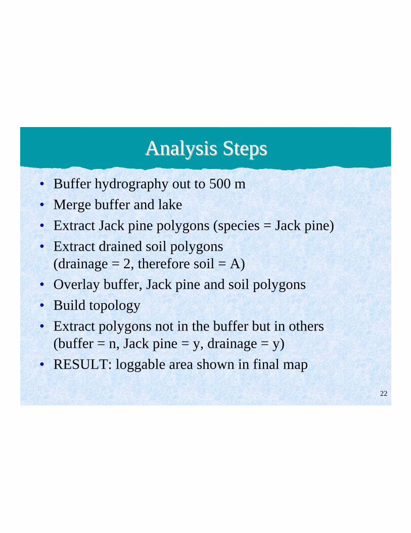
Analysis StepsAnalysis Steps

• Buffer hydrography out to 500 m

• Merge buffer and lake

• Extract Jack pine polygons (species = Jack pine)

• Extract drained soil polygons (drainage = 2, therefore soil = A)

• Overlay buffer, Jack pine and soil polygons

• Build topology

• Extract polygons not in the buffer but in others(buffer = n, Jack pine = y, drainage = y)

• RESULT: loggable area shown in final map

23

Vector GIS CapabilitiesVector GIS Capabilities

• Analysis functions with vector GIS are not quitethe same as with raster GIS– More operations deal with objects

– Measures such as area have to be calculated fromcoordinates of objects, instead of counting cells

• Some operations are more accurate– Estimates of area based on polygons more accurate

than counts of pixels

– Estimates of perimeter of polygon more accuratethan counting pixel boundaries on the edge of a zone

24

Vector GIS CapabilitiesVector GIS Capabilities

• Some operations are slower– Examples: Overlaying layers, finding

buffers

• Some operations are faster– Example: Finding patch through road

network

25

Simple DisplaySimple Display

• Using points and “arcs” can display thelocations of all objects stored

• Attributes and entity types can be displayed byvarying colors, line patterns and point symbols

• May only want to display a subset of the data– Example: want to display areas of urban land use

with some base map data• Select call political boundaries and highways, but only

areas that had urban land uses

26

Simple DisplaySimple Display (continued) (continued)

• How would the user do this?– E.g. One of the layers in a database is a “map” of

land use, called USE

– Area objects on this layer have several attributes

– One attribute, called CLASS, identifies the area’sland use

– For urban land use, it has the value “U”

– Need to extract boundaries for all areas that haveCLASS = “U”

27

Standard Query Language (SQL)Standard Query Language (SQL)

• Different systems use different ways offormulating queries

• SQL is used by many systems

• SQL phrase structure:– SELECT, attribute name(s)>FROM<table>

WHERE<condition statement>• Ex: SELECT FROM USE WHERE CLASS=“U”

• This selects only the objects for display - no attributes areretrieved by the query

28

SQL SQL (continued)(continued)

• SQL phrase structure (continued)– SQL examples using a list of student names

• SELECT name FROM list (selects all names)• SELECT name FROM list WHERE grade = “A” (selects

names of students receiving an “A”)• SELECT name FROM list WHERE cumgrade > 3.0

(selects names of students with a cumulative gpa greaterthan 3.0)

– SQL operators:• Relational: <, >, =, <= ,>=• Arithmetic: =, -, *, / (only on numeric fields• Boolean: and, or, not

29

Boolean OperatorsBoolean Operators

• Used to combine conditions– Ex: WHERE cumgrade > 3.0 AND grade = “A”

(selects students satisfying both conditions only)• Can have spatial meaning in GIS as well

– Ex: when two maps are overlayed, areas (polygons)that are superimposed have the “and” condition

• A spatial representation is used to illustrateBoolean operators in the study of logic, throughthe use of diagrams called Venn diagrams– Thus GIS area overlay is a geographical instance of

a Venn Diagram

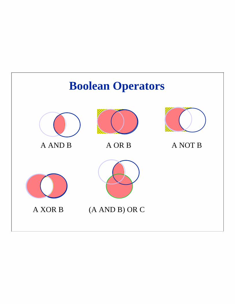
A AND B A OR B A NOT B

A XOR B (A AND B) OR C

Boolean Operators

31

SQL Extensions for Spatial QueriesSQL Extensions for Spatial Queries

• Some systems allow specifically spatial queriesto be handled under SQL– Ex: WITHIN operator

• SELECT <objects> WITHIN <specific area>

• The criteria for these spatial searches mayinclude searching within the radius of a point,within a bounding rectangle, or within anirregular polygon

32

Reclassify, Dissolve, & MergeReclassify, Dissolve, & Merge

• The operations are used frequently in workingwith area objects– These are used to aggregate areas based on

attributes

• Consider a soils map:– We wish to produce map of major soil types from a

layer that has polygons based on much more finelydefined classification scheme

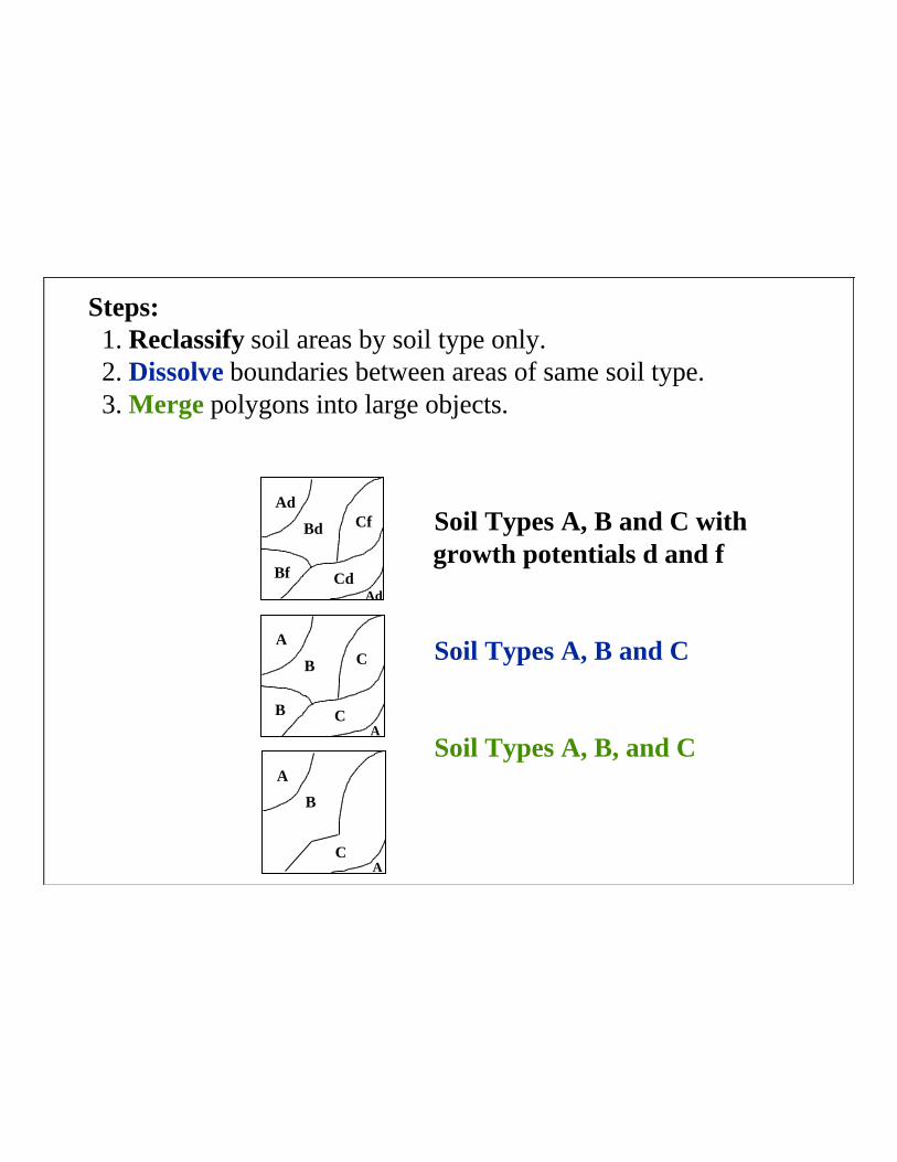
Steps: 1. Reclassify soil areas by soil type only. 2. Dissolve boundaries between areas of same soil type. 3. Merge polygons into large objects.

Soil Types A, B and C withgrowth potentials d and f

Soil Types A, B and C

Soil Types A, B, and C

Ad

Ad

Bd Cf

Bf Cd

A

B C

B CA

A

B

CA

34

Reclassify, Dissolve & Merge:Reclassify, Dissolve & Merge:

Forestry Example Forestry Example (1 of 2)(1 of 2)

• Consider a forestry GIS where the forest isdivided into “stands”, average size 10 ha:– Each stand carries a list of attributes, including tree

species and average tree age

– Attributes apply homogeneously to area of eachstand

– Boundary occurs between stands whenever at leastone attribute changes

35


Forestry Example Forestry Example (2 of 2)(2 of 2)

• Problem: identify all cuttable areas of white spruce– Assign new attribute “cuttable” to each stand

• Value = “y” if white spruce AND age > 50 years

• Value = “n” otherwise

– After assigning new attribute, all others can be dropped

• Now you wish to identify cuttable areas, eachmay be merger of several individual stands– Dissolve boundaries between polygons with

same value of “cuttable” attribute

– Merge polygons into larger objects

36


City Zoning ExampleCity Zoning Example

• Need to know how many individual landusezones have been created in the city and howthese are distribute geographically

• Each land parcel in the city has a zoningattribute attached to it

• Dissolve boundaries between parcels if thezoning is the same

• Result can be a map showing larger areas ofsimilar zoning classes

37

Topological OverlayTopological Overlay

• Suppose individual layers have planarenforcement (required in many systems, not all)

• When two layers are combined (“overlayed”,“superimposed”) the result must have planarenforcement as well– New intersection must be calculated and created

wherever two lines cross– A line across an area object creates two new area

objects• Topological overlay is the general name for

overlay followed by planar enforcement

38

Topological Overlay Topological Overlay (continued)(continued)

• Relationships are updated for the new,combined map

• Result may be information about relationships(new attributes) for the old (input) maps ratherthan the creation of new objects– Ex: overlay map of school districts on census tracts

• Result is map showing every school district/census tractcombination

• For each combo, the database contains an area objects• However, concern may be with obtaining the number of

overlapping census tracts as a new attribute of eachschool district rather than with new objects themselves

39

Point in PolygonPoint in Polygon

• Overlay point objects on areas, compute “iscontained in” relationship

• Result is a new attribute for each point

– Example: combine wells and planning districts, finddistrict containing each well

ID Owner ID County1 Dickinson A Black

2 Murray B Cole

3 Smith C Fall

4 McBran

5 Harris

ID County Owner1 Black Dickinson

2 Cole Murray

3 Cole Smith

4 Fall McBran

5 Fall Harris

Point in Polygon: ExamplePoint in Polygon: Example

12

3

4 5

12

3

4 5

A B

C

41

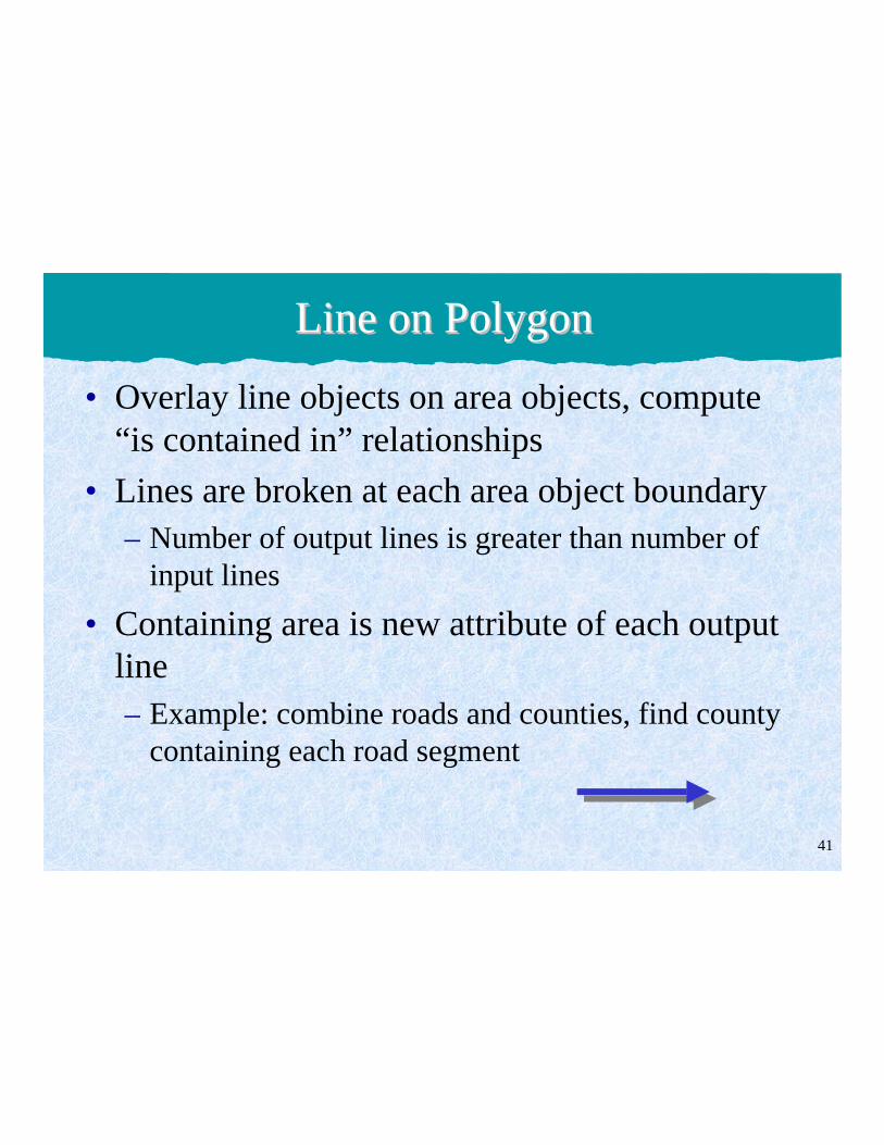
Line on PolygonLine on Polygon

• Overlay line objects on area objects, compute“is contained in” relationships

• Lines are broken at each area object boundary– Number of output lines is greater than number of

input lines

• Containing area is new attribute of each outputline– Example: combine roads and counties, find county

containing each road segment

Line onLine onPolygon:Polygon:ExampleExample

ID Highway1 35

2 22 ID County

3 35 A Black

4 60 B Cole

5 60 C Fall

6 35

7 82

8 35

ID Original Hwy County1 2 22 Black

2 2 22 Cole

3 1 35 Cole

4 3 35 Cole

5 4 60 Black

6 4 60 Cole

7 5 60 Cole

8 6 35 Cole

9 6 35 Fall

10 7 82 Fall

11 8 35 Fall

14 A B

C

2

35

67

8

1 2 3

45 678

910

11

43

Polygon on PolygonPolygon on Polygon(“Polygon Overlay”)(“Polygon Overlay”)

• Overlay two layers of area objects

• Boundaries are broken at each intersection

• Number of output areas likely greater than thetotal number of input areas– Example: input watershed boundaries, county

boundaries, output map of watershed/countycombinations

– After overlay we can recreate either of the inputlayers by dissolving and merging based on theattributes contributed by the input layer

44

Polygon on Polygon: ExamplePolygon on Polygon: Example

AB

C

1 2

3 4

53

7

1 2

468

ID WatershedID

CountyID

1 1 A

2 1 B

3 3 B

4 2 A

5 2 B

6 4 B

7 2 C

8 4 C

45

Example: Topological OverlayExample: Topological Overlay

• Wish to use those areas that are the best landfor timber harvesting

• After overlay, each original layer contributesattributes to the combined layer

• We get the final map by electing the desiredattributes of the combined layer– SELECT FROM OVERLAY WHERE Species =

“Jackpine” AND Soil = “C”

46

Spurious PolygonsSpurious Polygons

• During polygon overlay, many new and smallerpolygons are created, some of which may notrepresent true spatial variations

• See example

• The small, invalid polygons are called spuriousor sliver polygons and can be a major problemin polygon overlay

47

Sliver or Spurious PolygonsSliver or Spurious Polygons(page 1 of 3)

Township

Bellview

Royal

Southside

Skyline RiverSkyline River

School DistrictBoundaries

48


101

104

106105

Skyline River Skyline River

CensusBoundaries

103

102

49


101

104

106105

Skyline River Skyline River

Census Boundary

School DistrictBoundaries

SpuriousPolygons

103

102Township

Bellview

Royal

Southside

50

Spurious Polygons Spurious Polygons (continued)(continued)

• Spurious polygons arise when two lines are overlaidwhich are actually slightly different versions of thesame line– If the same line occurs on two input maps, the digitized

versions may be slightly different– In many cases the lines on the source maps have been

compiled from different sources, but are nevertheless thesame line on the ground

– Example: a road may be part of a county boundary, also theboundary between two fields or two soil types or twovegetation types

• The problem cannot be removed by more carefuldigitizing - more points simply lead to more slivers

51

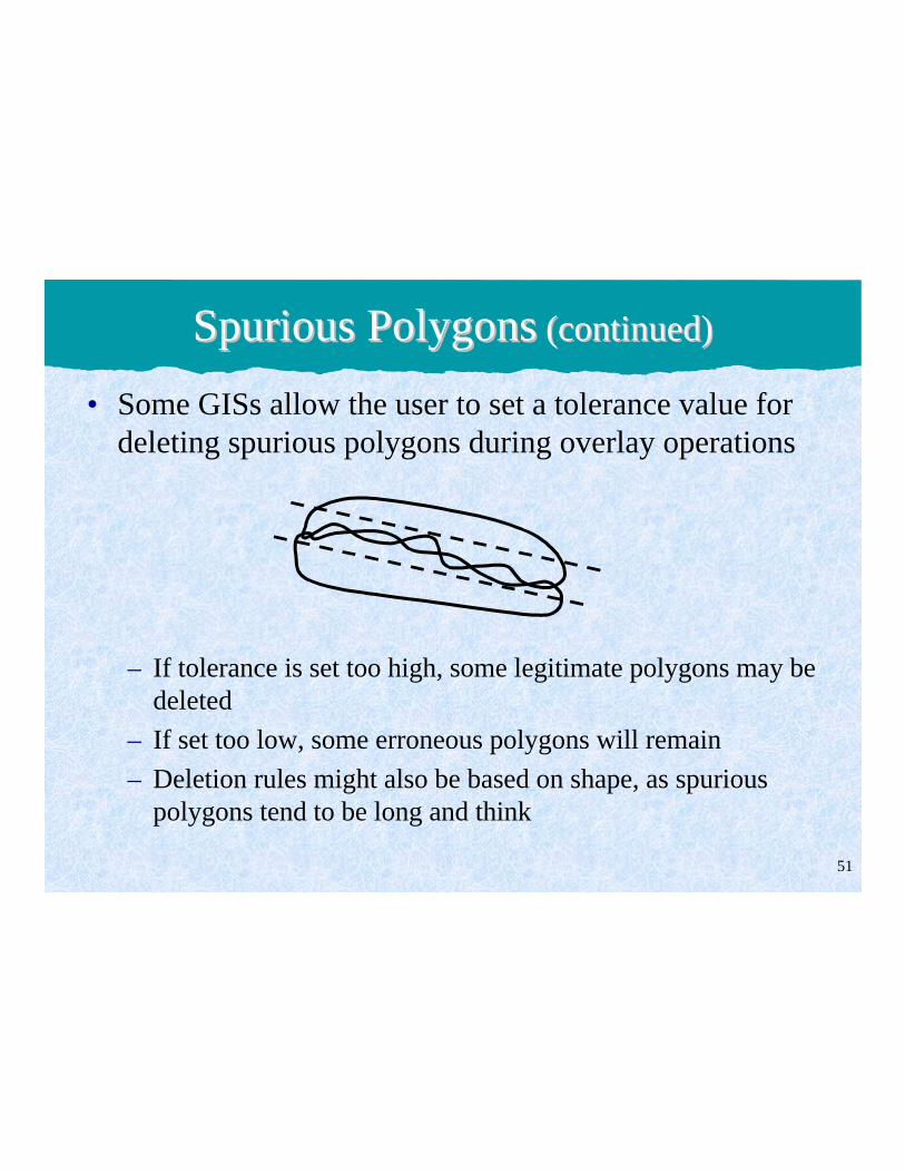
Spurious Polygons Spurious Polygons (continued)(continued)

• Some GISs allow the user to set a tolerance value fordeleting spurious polygons during overlay operations

– If tolerance is set too high, some legitimate polygons may bedeleted

– If set too low, some erroneous polygons will remain

– Deletion rules might also be based on shape, as spuriouspolygons tend to be long and think

52

BufferingBuffering

• A buffer can be constructed around a point, lineor area

• Buffering creates a new area, enclosing thebuffered object

• Applications in transportation forestry, resourcemanagement– Protected zones around lakes and streams– Zone of noise pollution around highways– Service zone around bus route (ex: 300 m walking

distance)– Groundwater pollution zone around waste site

53

Buffering

Buffering a Pointexample: All area withinone mile of the city.

Buffering a Lineexample: All areas within1000 meters of a road.

Buffering an Areaexample: All areas within500 meters of a wetlandsarea.

r

54

Buffering Buffering (continued)(continued)

• Options available for raster, such as a “friction”layer, do not exist for vector

• Sometimes, width of the buffer can bedetermined by an attribute of the object– Example: buffering residential buildings away from

a street network:• Three types of street (1,2,3 or major, secondary, tertiary)

with the setbacks being 600 feet from a major street, 200feet from a secondary street, and only 100 feet from atertiary street

55

Buffering Buffering (continued)(continued)

• Buffering is much more difficult in vector fromthe point of view of the programmer

• Problems with buffer operations may occurwhen buffering very convoluted lines or areas:

Documents

Tim Haithcoat University of Missouri Columbia - MSDISmsdis.missouri.edu/resources/intro_to_gis/pdf/Vector.pdf · Tim Haithcoat University of Missouri Columbia With materials from: