Three-way ANOVA Chapter

688 Chapter 22 • Three-Way ANOVA

ACONCEPTUALFOUNDATION

22C h a p t e r

Three-Way ANOVA

You will need to use the following from previous chapters:

Symbolsk: Number of independent groups in a one-way ANOVA

c: Number of levels (i.e., conditions) of an RM factorn: Number of subjects in each cell of a factorial ANOVA

NT: Total number of observations in an experiment

FormulasFormula 16.2: SSinter (by subtraction) also Formulas 16.3, 16.4, 16.5

Formula 14.3: SSbet or one of its components

ConceptsAdvantages and disadvantages of the RM ANOVA

SS components of the one-way RM ANOVASS components of the two-way ANOVA

Interaction of factors in a two-way ANOVA

So far I have covered two types of two-way factorial ANOVAs: two-way inde-pendent (Chapter 14) and the mixed design ANOVA (Chapter 16). There is onlyone more simple two-way ANOVA to describe: the two-way repeated measuresdesign. [There are other two-way designs, such as those including random-effects or nested factors, but they are not commonly used—see Hays (1994) fora description of some of these.] Just as the one-way RM ANOVA can bedescribed in terms of a two-way independent-groups ANOVA, the two-way RMANOVA can be described in terms of a three-way independent-groups ANOVA.This gives me a reason to describe the latter design next. Of course, the three-way factorial ANOVA is interesting in its own right, and its frequent use in thepsychological literature makes it an important topic to cover, anyway. I will dealwith the three-way independent-groups ANOVA and the two-way RM ANOVAin this section and the two types of three-way mixed designs in Section B.

Computationally, the three-way ANOVA adds nothing new to the proce-dure you learned for the two-way; the same basic formulas are used a greaternumber of times to extract a greater number of SS components from SStotal

(eight SSs for the three-way as compared with four for the two-way). However,anytime you include three factors, you can have a three-way interaction, andthat is something that can get quite complicated, as you will see. To give you amanageable view of the complexities that may arise when dealing with threefactors, I’ll start with a description of the simplest case: the 2 × 2 × 2 ANOVA.

A Simple Three-Way ExampleAt the end of Section B in Chapter 14, I reported the results of a publishedstudy, which was based on a 2 × 2 ANOVA. In that study one factor con-trasted subjects who had an alcohol-dependent parent with those who didnot. I’ll call this the alcohol factor and its two levels, at risk (of codepen-dency) and control. The other factor (the experimenter factor) also had twolevels; in one level subjects were told that the experimenter was an exploitiveperson, and in the other level the experimenter was described as a nurturingperson. All of the subjects were women. If we imagine that the experimentwas replicated using equal-sized groups of men and women, the original688

Cohen_Chapter22.j.qxd 8/23/02 11:56 M Page 688

two-way design becomes a three-way design with gender as the third factor.We will assume that all eight cells of the 2 × 2 × 2 design contain the samenumber of subjects. As in the case of the two-way ANOVA, unbalanced three-way designs can be difficult to deal with both computationally and concep-tually and therefore will not be discussed in this chapter (see Chapter 18,section A). The cell means for a three-factor experiment are often displayedin published articles in the form of a table, such as Table 22.1.

Section A • Conceptual Foundation 689

Nurturing Exploitive Row Mean

Control: Men 40 28 34Women 30 22 26Mean 35 25 30

At risk: Men 36 48 42Women 40 88 64Mean 38 68 53Column mean 36.5 46.5 41.5

Table 22.1

Figure 22.1

Graphing Three FactorsThe easiest way to see the effects of this experiment is to graph the cellmeans. However, putting all of the cell means on a single graph would not bean easy way to look at the three-way interaction. It is better to use twographs side by side, as shown in Figure 22.1. With a two-way design one hasto decide which factor is to be placed along the horizontal axis, leaving theother to be represented by different lines on the graph. With a three-waydesign one chooses both the factor to be placed along the horizontal axis andthe factor to be represented by different lines, leaving the third factor to berepresented by different graphs. These decisions result in six different waysthat the cell means of a three-way design can be presented.

Let us look again at Figure 22.1. The graph for the women shows the two-way interaction you would expect from the study on which it is based. Thegraph for the men shows the same kind of interaction, but to a considerablylesser extent (the lines for the men are closer to being parallel). This difference

80

70

60

50

40

30

20

Nurturing0 Exploitive

Control

At riskWomen Men

80

70

60

50

40

30

20


Control

At risk

Graph of Cell Means forData in Table 22.1


in amount of two-way interaction for men and women constitutes a three-wayinteraction. If the two graphs had looked exactly the same, the F ratio for thethree-way interaction would have been zero. However, that is not a necessarycondition. A main effect of gender could raise the lines on one graph relativeto the other without contributing to a three-way interaction. Moreover, aninteraction of gender with the experimenter factor could rotate the lines onone graph relative to the other, again without contributing to the three-wayinteraction. As long as the difference in slopes (i.e., the amount of two-wayinteraction) is the same in both graphs, the three-way interaction will be zero.

Simple Interaction EffectsA three-way interaction can be defined in terms of simple effects in a way thatis analogous to the definition of a two-way interaction. A two-way interactionis a difference in the simple main effects of one of the variables as you changelevels of the other variable (if you look at just the graph of the women in Fig-ure 22.1, each line is a simple main effect). In Figure 22.1 each of the twographs can be considered a simple effect of the three-way design—more specif-ically, a simple interaction effect. Each graph depicts the two-way interactionof alcohol and experimenter at one level of the gender factor. The three-wayinteraction can be defined as the difference between these two simple interac-tion effects. If the simple interaction effects differ significantly, the three-wayinteraction will be significant. Of course, it doesn’t matter which of the threevariables is chosen as the one whose different levels are represented as differ-ent graphs—if the three-way interaction is statistically significant, there will besignificant differences in the simple interaction effects in each case.

Varieties of Three-way InteractionsJust as there are many patterns of cell means that lead to two-way interac-tions (e.g., one line is flat while the other goes up or down, the two lines goin opposite directions, or the lines go in the same direction but with differ-ent slopes), there are even more distinct patterns in a three-way design. Per-haps the simplest is when all of the means are about the same, except forone, which is distinctly different. For instance, in our present example theresults might have shown no effect for the men (all cell means about 40), nodifference for the control women (both means about 40), and a mean of 40for at-risk women exposed to the nice experimenter. Then, if the mean for at-risk women with the exploitive experimenter were well above 40, therewould be a strong three-way interaction. This is a situation in which all threevariables must be at the “right” level simultaneously to see the effect—in thisvariation of our example the subject must be female and raised by an alco-hol-dependent parent and exposed to the exploitive experimenter to attain ahigh score. Not only might the three-way interaction be significant, but onecell mean might be significantly different from all of the other cell means,making an even stronger case that all three variables must be combinedproperly to see any effect (if you were sure that this pattern were going tooccur, you could test a contrast comparing the average of seven cell meansto the one you expect to be different and not bother with the ANOVA at all).

More often the results are not so clear-cut, but there is one cell meanthat is considerably higher than the others (as in Figure 22.1). This kind ofpattern is analogous to the ordinal interaction in the two-way case and tendsto cause all of the effects to be significant. On the other hand, a three-wayinteraction could arise because the two-way interaction reverses its patternwhen changing levels of the third variable (e.g., imagine that in Figure 22.1



the labels of the two lines were reversed for the graph of men but not for thewomen). This is analogous to the disordinal interaction in the two-way case.Or, the two-way interaction could be strong at one level of the third variableand much weaker (or nonexistent) at another level. Of course, there aremany other possible variations. And consider how much more complicatedthe three-way interaction can get when each factor has more than two levels(we will deal with a greater number of levels in Section B).

Fortunately, three-way (between-subjects) ANOVAs with many levels foreach factor are not common. One reason is a practical one: the number ofsubjects required. Even a design as simple as a 2 × 3 × 4 has 24 cells (to findthe number of cells, you just multiply the numbers of levels). If you want tohave at least 5 subjects per cell, 120 subjects are required. This is not animpractical study, but you can see how quickly the addition of more levelswould result in a required sample size that could be prohibitive.

Main EffectsIn addition to the three-way interaction there are three main effects to look at,one for each factor. To look at the gender main effect, for instance, just take theaverage of the scores for all of the men and compare it to the average of all ofthe women. If you have the cell means handy and the design is balanced, youcan average all of the cell means involving men and then all of the cell meansinvolving women. In Table 22.1, you can average the four cell means for themen (40, 28, 36, 48) to get 38 (alternatively, you could use the row means in theextreme right column and average 34 and 42 to get the same result). The aver-age for the women (30, 22, 40, 88) is 45. The means for the other main effectshave already been included in Table 22.1. Looking at the bottom row you cansee that the mean for the nurturing experimenter is 36.5 as compared to 46.5for the exploitive one. In the extreme right column you’ll find that the meanfor the control subjects is 30, as compared to 53 for the at-risk subjects.

Two-Way Interactions in Three-Way ANOVAsFurther complicating the three-way ANOVA is that, in addition to the three-way interaction and the three main effects, there are three two-way inter-actions to consider. In terms of our example there are the gender byexperimenter, gender by alcohol, and experimenter by alcohol interactions.We will look at the last of these first. Before graphing a two-way interactionin a three-factor design, you have to “collapse” (i.e., average) your scores overthe variable that is not involved in the two-way interaction. To graph the alco-hol by experimenter (A × B) interaction you need to average the men with thewomen for each combination of alcohol and experimenter levels (i.e., eachcell of the A × B matrix). These means have also been included in Table 22.1.

The graph of these cell means is shown in Figure 22.2. If you comparethis overall two-way interaction with the two-way interactions for the menand women separately (see Figure 22.1), you will see that the overall inter-action looks like an average of the two separate interactions; the amount ofinteraction seen in Figure 22.2 is midway between the amount of interactionfor the men and that amount for the women. Does it make sense to averagethe interactions for the two genders into one overall interaction? It does ifthey are not very different. How different is too different? The size of thethree-way interaction tells us how different these two two-way interactionsare. A statistically significant three-way interaction suggests that we shouldbe cautious in interpreting any of the two-way interactions. Just as a signif-icant two-way interaction tells us to look carefully at, and possible test, the




70

60

50

40

30

20


Control

At risk

Average of Men and Women

Graph of Cell Means inTable 22.1 after Averaging

Across Gender

Figure 22.2

simple main effects (rather than the overall main effects), a significant three-way interaction suggests that we focus on the simple interaction effects—thetwo-way interactions at each level of the third variable (which of the threeindependent variables is treated as the “third” variable is a matter of con-venience). Even if the three-way interaction falls somewhat short of signifi-cance, I would recommend caution in interpreting the two-way interactionsand the main effects, as well, whenever the simple interaction effects lookcompletely different and, perhaps, show opposite patterns.

So far I have been focusing on the two-way interaction of alcohol andexperimenter in our example, but this choice is somewhat arbitrary. The twogenders are populations that we are likely to have theories about, so it isoften meaningful to compare them. However, I can just as easily graph thethree-way interaction using “alcohol” as the third factor, as I have done inFigure 22.3a. To graph the overall two-way interaction of gender and exper-imenter, you can go back to Table 22.1 and average across the alcohol factor.For instance, the mean for men in the nurturing condition is found by aver-aging the mean for control group men in the nurturing condition (40) with

80

70

60

50

40

30

20


Women

Men

Control

80

70

60

50

40

30

20


Women

Men

At Risk

Graph of Cell Means inTable 22.1 Using the“Alcohol” Factor to

Distinguish the Panels

Figure 22.3a



Figure 22.3b

70

60

50

40

30

20


Women

Men

Average of Control and at Risk

Graph of Cell Means inTable 22.1 after Averaging

Across the “Alcohol”Factor

the mean for at-risk men in the nurturing condition (36), which is 38. Theoverall two-way interaction of gender and experimenter is shown in Figure22.3b. Note that once again the two-way interaction is a compromise. (Actu-ally, the two two-way interactions are not as different as they look; in bothcases the slope of the line for the women is more positive—or at least lessnegative). For completeness, I have graphed the three-way interaction usingexperimenter as the third variable, and the overall two-way interaction ofgender and alcohol in Figures 22.4a and 22.4b.

An Example of a Disordinal Three-Way InteractionIn the three-factor example I have been describing, it looks like all threemain effects and all three two-way interactions, as well as the three-wayinteraction, could easily be statistically significant. However, it is importantto note that in a balanced design all seven of these effects are independent;the seven F ratios do share the same error term (i.e., denominator), but thesizes of the numerators are entirely independent. It is quite possible to have

Figure 22.4a

80

70

60

50

40

30

20

Control0 At risk

Women

Men

Nurturing

80

70

60

50

40

30

20

Control0 At risk

Women

Men

Exploitive

Graph of Cell Means inTable 22.1 Using the

“Experimenter” Factor toDistinguish the Panels


a large three-way interaction while all of the other effects are quite small. Bychanging the means only for the men in our example, I will illustrate a large,disordinal interaction that obliterates two of the two-way interactions andtwo of the main effects. You can see in Figure 22.5a that this new three-wayinteraction is caused by a reversal of the alcohol by experimenter interactionfrom one gender to the other. In Figure 22.5b, you can see that the overallinteraction of alcohol by gender is now zero (the lines are parallel); the gen-der by experimenter interaction is also zero (not shown). On the other hand,the large gender by alcohol interaction very nearly obliterates the maineffects of both gender and alcohol (see Figure 22.5c). The main effect ofexperimenter is, however, large, as can be seen in Figure 22.5b.

An Example in which the Three-Way Interaction Equals Zero

Finally, I will change the means for the men once more to create an examplein which the three-way interaction is zero, even though the graphs for the


70

60

50

40

30

20

Control0 At risk

Women

Men

Average of Nurturing and Exploitive

Graph of Cell Means inTable 22.1 after AveragingAcross the “Experimenter”

Factor

Figure 22.4b

80

70

60

50

40

30

20

Nurturing0 Expoitive

Control

At risk

Women

80

70

60

50

40

30

20


Control

At risk

Men

Rearranging the CellMeans of Table 22.1 to

Depict a Disordinal 3-Way Interaction

Figure 22.5a


two genders do not look the same. In Figure 22.6, I created the means for themen by starting out with the women’s means and subtracting 10 from each(this creates a main effect of gender); then I added 30 only to the men’smeans that involved the nurturing condition. The latter change creates atwo-way interaction between experimenter and gender, but because itaffects both the men/nurturing means equally, it does not produce any three-way interaction. One way to see that the three-way interaction is zero in Fig-ure 22.6 is to subtract the slopes of the two lines for each gender. For thewomen the slope of the at-risk line is positive: 88 − 40 = 48. The slope of thecontrol line is negative: 22 − 30 = −8. The difference of the slopes is 48 − (−8) = 56.If we do the same for the men, we get slopes of 18 and −38, whose differenceis also 56. You may recall that a 2 × 2 interaction has only one df, and can besummarized by a single number, L, that forms the basis of a simple linearcontrast. The same is true for a 2 × 2 × 2 interaction or any higher-orderinteraction in which all of the factors have two levels. Of course, quantifyinga three-way interaction gets considerably more complicated when the fac-tors have more than two levels, but it is safe to say that if the two (or more)graphs are exactly the same, there will be no three-way interaction (they willcontinue to be identical, even if a different factor is chosen to distinguish the


Figure 22.5b

70

60

50

40

30

20


At risk

Control

Average of men and women

Regraphing Figure 22.5aafter Averaging Across

Gender

Figure 22.5c

70

60

50

40

30

20

Control0 At risk

MenWomen

Average of Nurturing and Exploitive

Regraphing Figure 22.5aafter Averaging Across

the “Experimenter”Factor


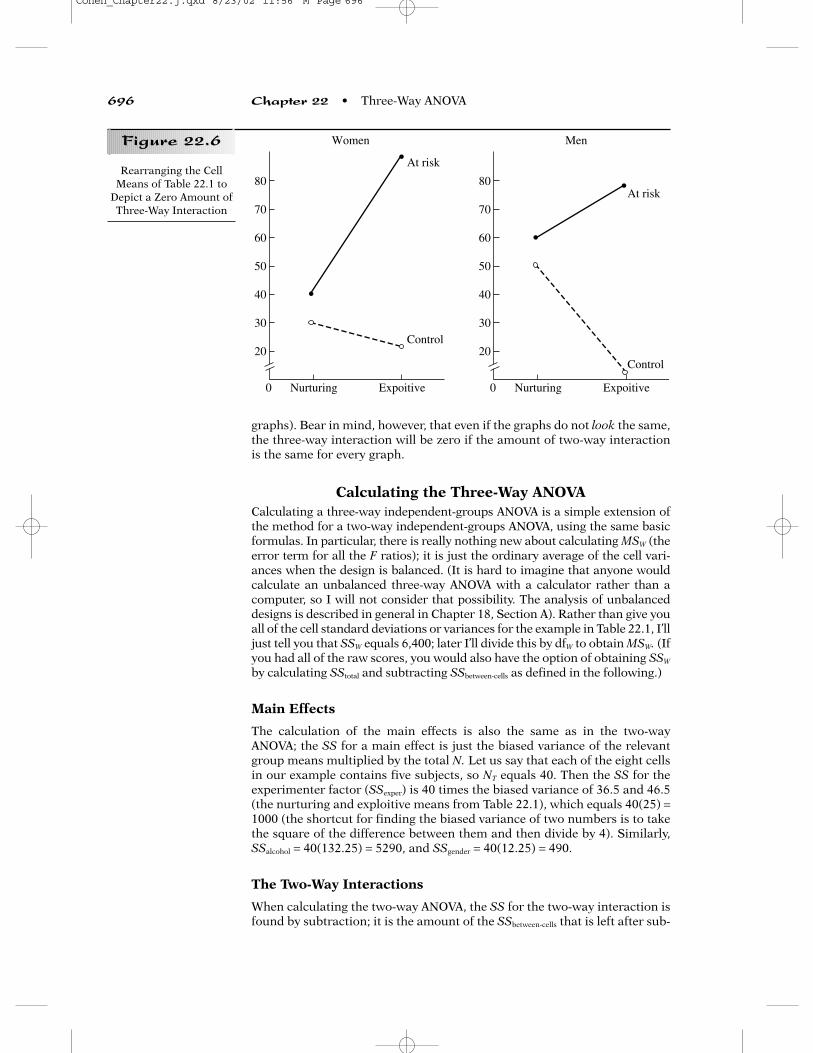
graphs). Bear in mind, however, that even if the graphs do not look the same,the three-way interaction will be zero if the amount of two-way interactionis the same for every graph.

Calculating the Three-Way ANOVACalculating a three-way independent-groups ANOVA is a simple extension ofthe method for a two-way independent-groups ANOVA, using the same basicformulas. In particular, there is really nothing new about calculating MSW (theerror term for all the F ratios); it is just the ordinary average of the cell vari-ances when the design is balanced. (It is hard to imagine that anyone wouldcalculate an unbalanced three-way ANOVA with a calculator rather than acomputer, so I will not consider that possibility. The analysis of unbalanceddesigns is described in general in Chapter 18, Section A). Rather than give youall of the cell standard deviations or variances for the example in Table 22.1, I’lljust tell you that SSW equals 6,400; later I’ll divide this by dfW to obtain MSW. (Ifyou had all of the raw scores, you would also have the option of obtaining SSW

by calculating SStotal and subtracting SSbetween-cells as defined in the following.)

Main Effects

The calculation of the main effects is also the same as in the two-wayANOVA; the SS for a main effect is just the biased variance of the relevantgroup means multiplied by the total N. Let us say that each of the eight cellsin our example contains five subjects, so NT equals 40. Then the SS for theexperimenter factor (SSexper) is 40 times the biased variance of 36.5 and 46.5(the nurturing and exploitive means from Table 22.1), which equals 40(25) =1000 (the shortcut for finding the biased variance of two numbers is to takethe square of the difference between them and then divide by 4). Similarly,SSalcohol = 40(132.25) = 5290, and SSgender = 40(12.25) = 490.

The Two-Way Interactions

When calculating the two-way ANOVA, the SS for the two-way interaction isfound by subtraction; it is the amount of the SSbetween-cells that is left after sub-


80

70

60

50

40

30

20


Control

At risk

Women

80

70

60

50

40

30

20


Control

At risk

Men

Rearranging the CellMeans of Table 22.1 to

Depict a Zero Amount ofThree-Way Interaction

Figure 22.6


tracting the SSs for the main effects. Similarly, the three-way interaction SSis the amount left over after subtracting the SSs for the main effects and theSSs for all the two-way interactions from the overall SSbetween-cells. However,finding the SSs for the two-way interactions in a three-way design gets a lit-tle tricky. In addition to the overall SSbetween-cells, we must also calculate someintermediate “two-way” SSbetween terms.

To keep track of these I will have to introduce some new subscripts. Theoverall SSbetween-cells is based on the variance of all the cell means, so no factorsare “collapsed,” or averaged over. Representing gender as G, alcohol as A, andexperimenter as E, the overall SSbetween-cells will be written as SSGAE. We willalso need to calculate an SSbetween after averaging over gender. This is based onthe four means (included in Table 22.1) I used to graph the alcohol by exper-imenter interaction and will be represented by SSAE. Because the design isbalanced, you can take the simple average of the appropriate male cell meanand female cell mean in each case. Note that SSAE is not the SS for the alco-hol by experimenter interaction because it also includes the main effects ofthose two factors. In similar fashion, we need to find SSGA from the meansyou get after averaging over the experimenter factor and SSGE by averagingover the alcohol factor. Once we have calculated these four SSbetween terms, allof the SSs we need for the three-way ANOVA can be found by subtraction.

Let’s begin with the calculation of SSGAE; the biased variance of the eightcell means is 366.75, so SSGAE = 40(366.75) = 14,670. The means for SSAE are35, 25, 38, 68, and their biased variance equals 257.75, so SSAE = 10,290. SSGA

is based on the following means: 34, 26, 42, 64, so SSGA = 40(200.75) = 8,030.Finally, SSGE, based on means of 38, 38, 35, 55, equals 2,490.

Next we find the SSs for each two-way interaction:

SSA × E = SSAE − SSalcohol − SSexper = 10,290 − 5,290 − 1,000 = 4,000SSG × A = SSGA − SSgender − SSalcohol = 8,030 − 490 − 5,290 = 2,250SSG × E = SSGE − SSgender − SSexper = 2,490 − 490 − 1,000 = 1,000

Finally, the SS for the three-way interaction (SSG × A × E) equals

SSGAE − SSA × E − SSG × A − SSG × E − SSgender − SSalcohol − SSexper

= 14,670 − 4,000 − 2,250 − 1,000 − 490 − 5,290 − 1,000 = 640

Formulas for the General Case

It is traditional to assign the letters A, B, and, C to the three independentvariables in the general case; variables D, E, and so forth, can then be addedto represent a four-way, five-way, or higher ANOVA. I’ll assume that the fol-lowing components have already been calculated using Formula 14.3applied to the appropriate means: SSA, SSB, SSC, SSAB, SSAC, SSBC, SSABC. Inaddition, I’ll assume that SSW has also been calculated, either by averagingthe cell variances and multiplying by dfW or by subtracting SSABC from SStotal.The remaining SS components are found by Formula 22.1:

a. SSA × B = SSAB − SSA − SSB Formula 22.1b. SSA × C = SSAC − SSA − SSC

c. SSB × C = SSBC − SSB − SSC

d. SSA × B × C = SSABC − SSA × B − SSB × C − SSA × C − SSA − SSB − SSC

At the end of the analysis, SStotal (whether or not it has been calculatedseparately) has been divided into eight components: SSA, SSB, SSC, the fourinteractions listed in Formula 22.1, and SSW. Each of these is divided by itscorresponding df to form a variance estimate, MS. Using a to represent the



number of levels of the A factor, b for the B factor, c for the C factor, and nfor the number of subjects in each cell, the formulas for the df componentsare as follows:

a. dfA = a − 1 Formula 22.2b. dfB = b − 1c. dfC = c − 1d. dfA × B = (a − 1)(b − 1)e. dfA × C = (a − 1)(c − 1)f. dfB × C = (b − 1)(c − 1)g. dfA × B × C = (a − 1)(b − 1)(c − 1)h. dfW = abc (n − 1)

Completing the Analysis for the Example

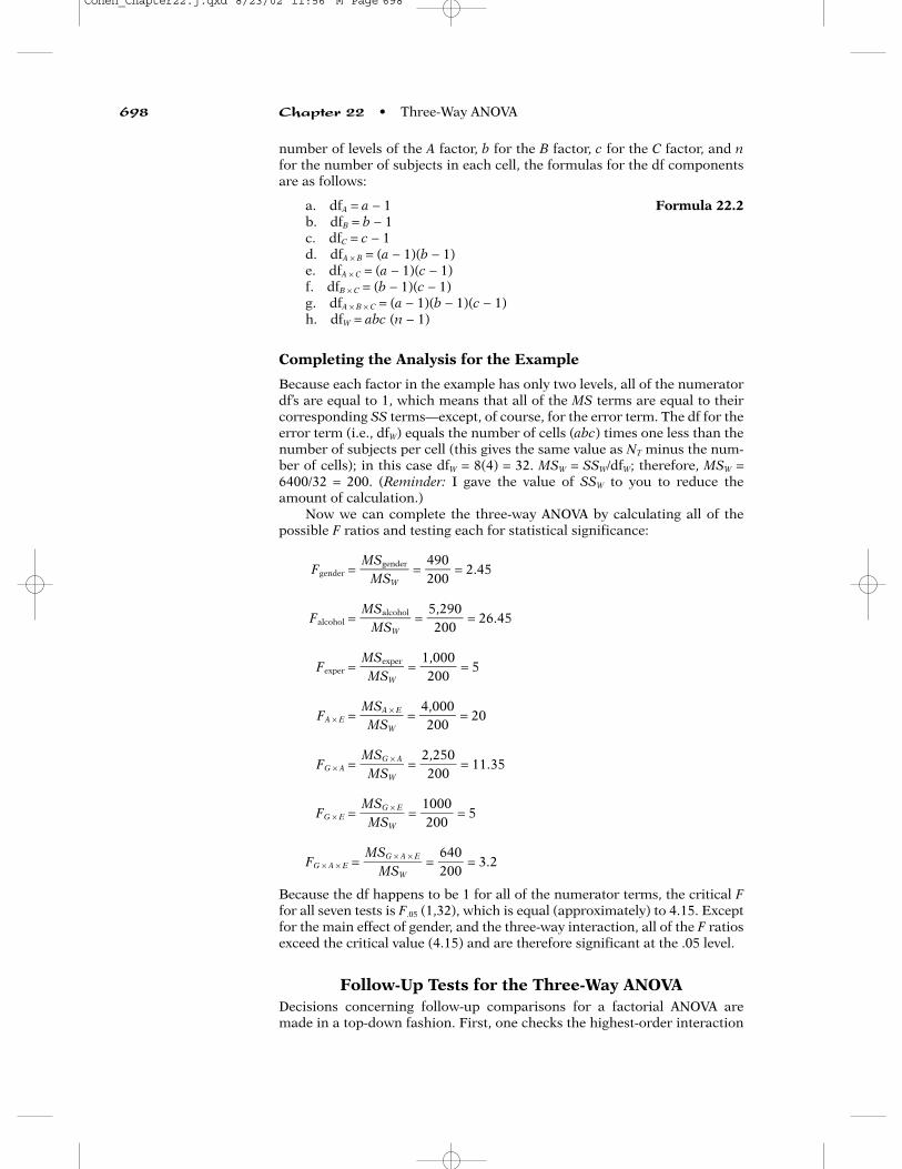
Because each factor in the example has only two levels, all of the numeratordf’s are equal to 1, which means that all of the MS terms are equal to theircorresponding SS terms—except, of course, for the error term. The df for theerror term (i.e., dfW) equals the number of cells (abc) times one less than thenumber of subjects per cell (this gives the same value as NT minus the num-ber of cells); in this case dfW = 8(4) = 32. MSW = SSW/dfW; therefore, MSW =6400/32 = 200. (Reminder: I gave the value of SSW to you to reduce theamount of calculation.)

Now we can complete the three-way ANOVA by calculating all of thepossible F ratios and testing each for statistical significance:

Fgender = = = 2.45

Falcohol = = = 26.45

Fexper = = = 5

FA × E = = = 20

FG × A = = = 11.35

FG × E = = = 5

FG × A × E = = = 3.2

Because the df happens to be 1 for all of the numerator terms, the critical Ffor all seven tests is F.05 (1,32), which is equal (approximately) to 4.15. Exceptfor the main effect of gender, and the three-way interaction, all of the F ratiosexceed the critical value (4.15) and are therefore significant at the .05 level.

Follow-Up Tests for the Three-Way ANOVADecisions concerning follow-up comparisons for a factorial ANOVA aremade in a top-down fashion. First, one checks the highest-order interaction

640�200

MSG × A × E��

MSW

1000�200

MSG × E�

MSW

2,250�200

MSG × A�

MSW

4,000�200

MSA × E�

MSW

1,000�200

MSexper�

MSW

5,290�200

MSalcohol�

MSW

490�200

MSgender�

MSW



for significance; in a three-way ANOVA it is the three-way interaction. (Two-way interactions are the simplest possible interactions and are called first-order interactions; three-way interactions are known as second-orderinteractions, etc.) If the highest interaction is significant, the post hoc testsfocus on the various simple effects or interaction contrasts, followed byappropriate cell-to-cell comparisons. In a three-way ANOVA in which thethree-way interaction is not significant, as in the present example, attentionturns to the three two-way interactions. Although all of the two-way interac-tions are significant in our example, the alcohol by experimenter interactionis the easiest to interpret because it replicates previous results.

It would be appropriate to follow up the significant alcohol by experi-menter interaction with four t tests (e.g., one of the relevant t tests woulddetermine whether at-risk subjects differ significantly from controls in theexploitive condition). Given the disordinal nature of the interaction (see Fig-ure 22.2), it is likely that the main effects would simply be ignored. A similarapproach would be taken to the two other significant two-way interactions.Thus, all three main effects would be regarded with caution. Note thatbecause all of the factors are dichotomous, there would be no follow-up teststo perform on significant main effects, even if none of the interactions weresignificant. With more than two levels for some or all of the factors, itbecomes possible to test partial interactions, and significant main effects forfactors not involved in significant interactions can be followed by pairwiseor complex comparisons, as described in Chapter 14, Section C. I will illus-trate some of the complex planned and post hoc comparisons for the three-way design in Section B.

Types of Three-Way DesignsCases involving significant three-way interactions and factors with morethan two levels will be considered in the context of mixed designs in SectionB. However, before we turn to mixed designs, let us look at some of the typ-ical situations in which three-way designs with no repeated measures arise.One situation involves three experimental manipulations for which repeatedmeasures are not feasible. For instance, subjects perform a repetitive task inone of two conditions: They are told that their performance is being meas-ured or that it is not. In each condition half of the subjects are told that per-formance on the task is related to intelligence, and the other half are toldthat it is not. Finally, within each of the four groups just described, half thesubjects are treated respectfully and half are treated rudely. The work outputof each subject can then be analyzed by a 2 × 2 × 2 ANOVA.

Another possibility involves three grouping variables, each of whichinvolves selecting subjects whose group is already determined. For instance, agroup of people who exercise regularly and an equal-sized group of those whodon’t are divided into those high and those relatively low on self-esteem (by amedian split). If there are equal numbers of men and women in each of thefour cells, we have a balanced 2 × 2 × 2 design. More commonly one or two ofthe variables involve experimental manipulations and two or one involvegrouping variables. The example calculated earlier in this section involved twogrouping variables (gender and having an alcohol-dependent parent or not)and one experimental variable (nurturing vs. exploitive experimenter).

To devise an interesting example with two experimental manipulationsand one grouping variable, start with two experimental factors that areexpected to interact (e.g., one factor is whether or not the subjects are toldthat performance on the experimental task is related to intelligence, and theother factor is whether or not the group of subjects run together will know



each other’s final scores). Then, add a grouping variable by comparing sub-jects who are either high or low on self-esteem, need for achievement, orsome other relevant aspect of personality. If the two-way interaction differssignificantly between the two groups of subjects, the three-way interactionwill be significant.

The Two-Way RM ANOVAOne added benefit of learning how to calculate a three-way ANOVA is thatyou now know how to calculate a two-way ANOVA in which both factorsinvolve repeated measures. In Chapter 15, I showed you that the SS compo-nents of a one-way RM design are calculated as though the design were atwo-way independent-groups ANOVA with no within-cell variability. Simi-larly, a two-way RM ANOVA is calculated just as shown in the preceding forthe three-way independent-groups ANOVA, with the following modifica-tions: (1) One of the three factors is the subjects factor—each subject repre-sents a different level of the subjects factor, (2) the main effect of subjects isnot tested, and there is no MSW error term, (3) each of the two main effectsthat is tested uses the interaction of that factor with the subjects factor as theerror term, and (4) the interaction of the two factors of interest is tested byusing as the error term the interaction of all three factors (i.e., including thesubjects factor). If one RM factor is labeled Q and the other factor, R, and weuse S to represent the subjects factor, the equations for the three F ratios canbe written as follows:

FQ = , FR = FQ × R =

Higher-Order ANOVAThis text will not cover factorial designs of higher order than the three-wayANOVA. Although higher-order ANOVAs can be difficult to interpret, no newprinciples are introduced. The four-way ANOVA produces 15 different Fratios to test: four main effects, 6 two-way interactions, 4 three-way interac-tions, and 1 four-way interaction. Testing each of these 15 effects at the .05level raises serious concerns about the increased risk of Type I errors. Usu-ally, all of the F ratios are not tested; specific hypotheses should guide theselection of particular effects to test. Of course, the potential for an inflatedrate of Type I errors only increases as factors are added. In general, an N-wayANOVA produces 2N − 1 F ratios that can be tested for significance.

In the next section I will delve into more complex varieties of the three-way ANOVA—in particular those that include repeated measures on one ortwo of the factors.

1. To display the cell means of a three-way factorial design, it is convenientto create two-way graphs for each level of the third variable and placethese graphs side by side (you have to decide which of the three vari-ables will distinguish the graphs and which of the two remaining vari-ables will be placed along the X axis of each graph). Each two-way graphdepicts a simple interaction effect; if the simple interaction effects aresignificantly different from each other, the three-way interaction will besignificant.

2. Three-way interactions can occur in a variety of ways. The interaction oftwo of the factors can be strong at one level of the third factor and close

MSQ × R��MXQ × R × S

MSR�MSR × S

MSQ�MSQ × S


ASUMMARY


to zero at a different level (or even stronger at a different level). Thedirection of the two-way interaction can reverse from one level of thethird variable to another. Also, a three-way interaction can arise whenall of the cell means are similar except for one.

3. The main effects of the three-way ANOVA are based on the means ateach level of one of the factors, averaging across the other two. A two-way interaction is the average of the separate two-way interactions(simple interaction effects) at each level of the third factor. A two-wayinteraction is based on a two-way table of means created by averagingacross the third factor.

4. The error term for the three-way ANOVA, MSW, is a simple extension ofthe error term for a two-way ANOVA; in a balanced design, it is the sim-ple average of all of the cell variances. All of the SSbetween components arefound by Formula 14.3, or by subtraction using Formula 22.1. There areseven F ratios that can be tested for significance: the three main effects,three two-way interactions, and the three-way interaction.

5. Averaging simple interaction effects together to create a two-way inter-action is reasonable only if these effects do not differ significantly. Ifthey do differ, follow-up tests usually focus on the simple interactioneffects themselves or particular 2 × 2 interaction contrasts. If the three-way interaction is not significant, but a two-way interaction is, the sig-nificant two-way interaction is explored as in a two-way ANOVA—withsimple main effects or interaction contrasts. Also, when the three-wayinteraction is not significant, any significant main effect can be followedup in the usual way if that variable is not involved in a significant two-way interaction.

6. All three factors in a three-way ANOVA can be grouping variables (i.e.,based on intact groups), but this is rare. It is more common to have justone grouping variable and compare the interaction of two experimentalfactors among various subgroups of the population. Of course, all threefactors can involve experimental manipulations.

7. The two-way ANOVA in which both factors involve repeated measures isanalyzed as a three-way ANOVA, with the different subjects serving asthe levels of the third factor. The error term for each RM factor is theinteraction of that factor with the subject factor; the error term for theinteraction of the two RM factors is the three-way interaction.

8. In an N-way factorial ANOVA, there are 2N − 1 F ratios that can be tested.The two-way interaction is called a first-order interaction, the three-wayis a second-order interaction, and so forth.


1. Imagine an experiment in which each sub-ject is required to use his or her memories tocreate one emotion: either happiness, sad-ness, anger, or fear. Within each emotiongroup, half of the subjects participate in arelaxation exercise just before the emotioncondition, and half do not. Finally, half thesubjects in each emotion/relaxation condi-tion are run in a dark, sound-proof chamber,and the other half are run in a normally litroom. The dependent variable is the subject’s

systolic blood pressure when the subject sig-nals that the emotion is fully present. Thedesign is balanced, with a total of 128 sub-jects. The results of the three-way ANOVA forthis hypothetical experiment are as follows:SSemotion = 223.1, SSrelax = 64.4, SSdark = 31.6,SSemo × rel = 167.3, SSemo × dark = 51.5; SSrel × dark =127.3, and SSemo × rel × dark = 77.2. The total sumof squares is 2,344.a. Calculate the seven F ratios, and test each

for significance.

EXERCISES


b. Calculate partial eta squared for each ofthe three main effects (use Formula 14.9).Are any of these effects at least moderatein size?

2. In this exercise there are 20 subjects in eachcell of a 3 × 3 × 2 design. The levels of the firstfactor (location) are urban, suburban, andrural. The levels of the second factor are nosiblings, one or two siblings, and more thantwo siblings. The third factor has only twolevels: presently married and not presentlymarried. The dependent variable is the num-ber of close friends that each subject reportshaving. The cell means are as follows:

a. Given that SSW equals 1,094, complete thethree-way ANOVA, and present yourresults in a summary table.

b. Draw a graph of the means for Location ×Number of Siblings (averaging across mar-ital status). Describe the nature of theinteraction.

c. Using the means from part b, test the sim-ple effect of number of siblings at eachlocation.

3. Seventy-two patients with agoraphobia arerandomly assigned to one of four drug condi-tions: SSRI (e.g., Prozac), tricyclic antidepres-sant (e.g., Elavil), antianxiety (e.g., Xanax), ora placebo (offered as a new drug for agora-phobia). Within each drug condition, a thirdof the patients are randomly assigned to eachof three types of psychotherapy: psychody-namic, cognitive/behavioral, and group. Thesubjects are assigned so that half the subjectsin each drug/therapy group are also de-pressed, and half are not. After 6 months oftreatment, the severity of agoraphobia ismeasured for each subject (30 is the maxi-mum possible phobia score); the cell means(n = 3) are as follows:a. Given that SSW equals 131, complete the

three-way ANOVA, and present your resultsin a summary table.

b. Draw a graph of the cell means, with sep-arate panels for depressed and notdepressed. Describe the nature of thetherapy × drug interaction in each panel.Does there appear to be a three-way inter-action? Explain.

c. Given your results in part a, describe a setof follow-up tests that would be justifi-able.

d. Optional: Test the 2 × 2 × 2 interactioncontrast that results from deleting Grouptherapy and the SSRI and placebo condi-tions from the analysis (extend the tech-niques of Chapter 13, Section B, andChapter 14, Section C).

4. An industrial psychologist is studying therelation between motivation and productiv-ity. Subjects are told to perform as manyrepetitions of a given clerical task as theycan in a 1-hour period. The dependent vari-able is the number of tasks correctly per-formed. Sixteen subjects participated in theexperiment for credit toward a requirementof their introductory psychology course(credit group). Another 16 subjects wererecruited from other classes and paid $10for the hour (money group). All subjectsperformed a small set of similar clericaltasks as practice before the main study; ineach group (credit or money) half the sub-jects (selected randomly) were told they hadperformed unusually well on the practicetrials (positive feedback), and half were toldthey had performed poorly (negative feed-back). Finally, within each of the fourgroups created by the manipulations justdescribed, half of the subjects (at random)were told that performing the tasks quicklyand accurately was correlated with otherimportant job skills (self motivation),whereas the other half were told that goodperformance would help the experiment(other motivation). The data appear in thefollowing table:


Urban Suburban Rural

No SiblingsMarried 1.9 3.1 2.0Not Married 4.7 5.7 3.5

1 or 2 SiblingsMarried 2.3 3.0 3.3Not Married 4.5 5.3 4.6

2 or more SiblingsMarried 3.2 4.5 2.9Not Married 3.9 6.2 4.6

SSRI Tricyclic Antianxiety Placebo

PsychodynamicNot Depressed 10 11.5 19.0 22.0Depressed 8.7 8.7 14.5 19.0

Cog/BehavNot Depressed 9.5 11.0 12.0 17.0Depressed 10.3 14.0 10.0 16.5

GroupNot Depressed 11.6 12.6 19.3 13.0Depressed 9.7 12.0 17.0 11.0


a. Perform a three-way ANOVA on the data.Test all seven F ratios for significance, andpresent your results in a summary table.

b. Use graphs of the cell means to help youdescribe the pattern underlying eacheffect that was significant in part a.

c. Based on the results in part a, what posthoc tests would be justified?

5. Imagine that subjects are matched in blocksof three based on height, weight, and otherphysical characteristics; six blocks areformed in this way. Then the subjects in eachblock are randomly assigned to three differ-

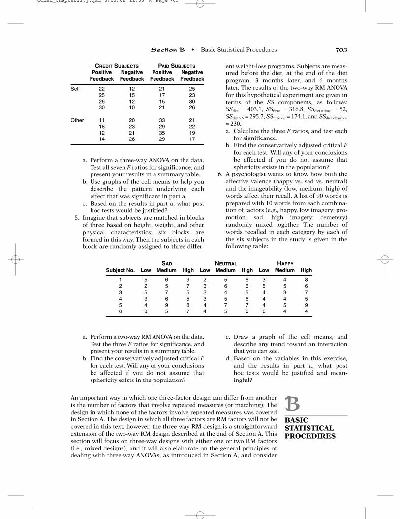
ent weight-loss programs. Subjects are meas-ured before the diet, at the end of the diet program, 3 months later, and 6 months later. The results of the two-way RM ANOVAfor this hypothetical experiment are given interms of the SS components, as follows: SSdiet = 403.1, SStime = 316.8, SSdiet × time = 52,SSdiet × S = 295.7, SStime × S = 174.1, and SSdiet × time × S

= 230.a. Calculate the three F ratios, and test each

for significance.b. Find the conservatively adjusted critical F

for each test. Will any of your conclusionsbe affected if you do not assume thatsphericity exists in the population?

6. A psychologist wants to know how both theaffective valence (happy vs. sad vs. neutral)and the imageability (low, medium, high) ofwords affect their recall. A list of 90 words isprepared with 10 words from each combina-tion of factors (e.g., happy, low imagery: pro-motion; sad, high imagery: cemetery)randomly mixed together. The number ofwords recalled in each category by each ofthe six subjects in the study is given in thefollowing table:

a. Perform a two-way RM ANOVA on the data.Test the three F ratios for significance, andpresent your results in a summary table.

b. Find the conservatively adjusted critical Ffor each test. Will any of your conclusionsbe affected if you do not assume thatsphericity exists in the population?

c. Draw a graph of the cell means, anddescribe any trend toward an interactionthat you can see.

d. Based on the variables in this exercise,and the results in part a, what post hoc tests would be justified and mean-ingful?

Section B • Basic Statistical Procedures 703

CREDIT SUBJECTS PAID SUBJECTSPositive Negative Positive Negative

Feedback Feedback Feedback Feedback

Self 22 12 21 2525 15 17 2326 12 15 3030 10 21 26

Other 11 20 33 2118 23 29 2212 21 35 1914 26 29 17

SAD NEUTRAL HAPPYSubject No. Low Medium High Low Medium High Low Medium High

1 5 6 9 2 5 6 3 4 82 2 5 7 3 6 6 5 5 63 5 7 5 2 4 5 4 3 74 3 6 5 3 5 6 4 4 55 4 9 8 4 7 7 4 5 96 3 5 7 4 5 6 6 4 4

An important way in which one three-factor design can differ from anotheris the number of factors that involve repeated measures (or matching). Thedesign in which none of the factors involve repeated measures was coveredin Section A. The design in which all three factors are RM factors will not becovered in this text; however, the three-way RM design is a straightforwardextension of the two-way RM design described at the end of Section A. Thissection will focus on three-way designs with either one or two RM factors(i.e., mixed designs), and it will also elaborate on the general principles ofdealing with three-way ANOVAs, as introduced in Section A, and consider

BBASICSTATISTICALPROCEDIRES


the complexities of interactions and post hoc tests when the factors havemore than two levels each.

One RM FactorI will begin with a three-factor design in which there are repeated measureson only one of the factors. The ANOVA for this design is not much morecomplicated than the two-way mixed ANOVA described in the previouschapter—for instance, there are only two different error terms. Such designsarise frequently in psychological research. One simple way to arrive at sucha design is to start with a two-way ANOVA with no repeated measures. Forinstance, patients with two different types of anxiety disorders (generalizedanxiety vs. specific phobias) are treated with two different forms of psy-chotherapy (psychodynamic vs. behavioral). The third factor is added bymeasuring the patients’ anxiety at several points in time (e.g., beginning oftherapy, end of therapy, several months after therapy has stopped); I willrefer to this factor simply as time.

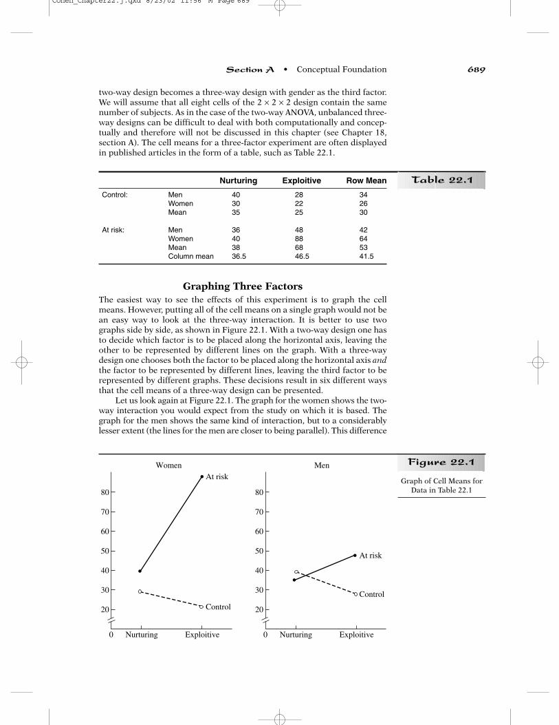
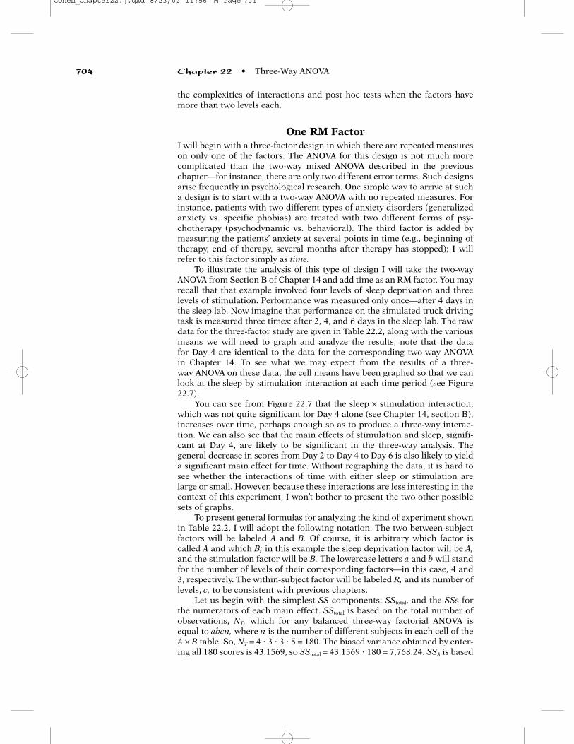
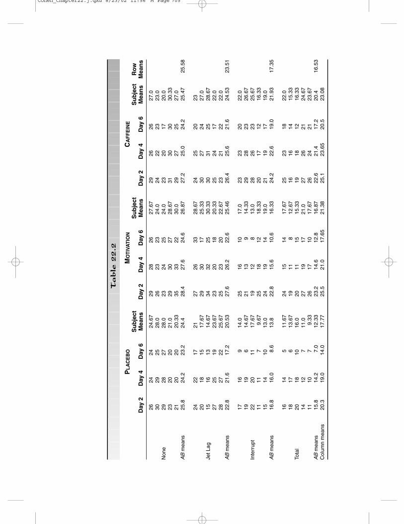
To illustrate the analysis of this type of design I will take the two-wayANOVA from Section B of Chapter 14 and add time as an RM factor. You mayrecall that that example involved four levels of sleep deprivation and threelevels of stimulation. Performance was measured only once—after 4 days inthe sleep lab. Now imagine that performance on the simulated truck drivingtask is measured three times: after 2, 4, and 6 days in the sleep lab. The rawdata for the three-factor study are given in Table 22.2, along with the variousmeans we will need to graph and analyze the results; note that the data for Day 4 are identical to the data for the corresponding two-way ANOVA in Chapter 14. To see what we may expect from the results of a three-way ANOVA on these data, the cell means have been graphed so that we canlook at the sleep by stimulation interaction at each time period (see Figure22.7).

You can see from Figure 22.7 that the sleep × stimulation interaction,which was not quite significant for Day 4 alone (see Chapter 14, section B),increases over time, perhaps enough so as to produce a three-way interac-tion. We can also see that the main effects of stimulation and sleep, signifi-cant at Day 4, are likely to be significant in the three-way analysis. Thegeneral decrease in scores from Day 2 to Day 4 to Day 6 is also likely to yielda significant main effect for time. Without regraphing the data, it is hard tosee whether the interactions of time with either sleep or stimulation arelarge or small. However, because these interactions are less interesting in thecontext of this experiment, I won’t bother to present the two other possiblesets of graphs.

To present general formulas for analyzing the kind of experiment shownin Table 22.2, I will adopt the following notation. The two between-subjectfactors will be labeled A and B. Of course, it is arbitrary which factor iscalled A and which B; in this example the sleep deprivation factor will be A,and the stimulation factor will be B. The lowercase letters a and b will standfor the number of levels of their corresponding factors—in this case, 4 and3, respectively. The within-subject factor will be labeled R, and its number oflevels, c, to be consistent with previous chapters.

Let us begin with the simplest SS components: SStotal, and the SSs forthe numerators of each main effect. SStotal is based on the total number ofobservations, NT, which for any balanced three-way factorial ANOVA isequal to abcn, where n is the number of different subjects in each cell of theA × B table. So, NT = 4 � 3 � 3 � 5 = 180. The biased variance obtained by enter-ing all 180 scores is 43.1569, so SStotal = 43.1569 � 180 = 7,768.24. SSA is based



PL

AC

EB

OM

OT

IVA

TIO

NC

AF

FE

INE

Su

bje

ctS

ub

ject

Su

bje

ctR

ow

Day

2D

ay 4

Day

6M

ean

sD

ay 2

Day

4D

ay 6

Mea

ns

Day

2D

ay 4

Day

6M

ean

sM

ean

s

2624

2424

.67

2928

2627

.67

2926

2627

.030

2925

28.0

2623

2324

.024

2223

23.0

Non

e29

2827

28.0

2324

2524

.023

2017

20.0

2320

2021

.029

3027

28.6

731

3030

30.3

321

2020

20.3

335

3322

30.0

2927

2527

.0A

Bm

eans

25.8

24.2

23.2

24.4

28.4

27.6

24.6

26.8

727

.225

.024

.225

.47

25.5

8

2422

1721

2726

3328

.67

2425

2023

2018

1517

.67

2930

1725

.33

3027

2427

.0Je

t Lag

1516

1314

.67

3432

2530

.33

3031

2528

.67

2725

1923

.67

2320

1820

.33

2524

1722

.028

2722

25.6

725

2320

22.6

723

2122

22.0

AB

mea

ns22

.821

.617

.220

.53

27.6

26.2

22.6

25.4

626

.425

.621

.624

.53

23.5

1

1716

914

.025

1610

17.0

2323

2022

.019

196

14.6

721

139

14.3

329

2823

26.6

7In

terr

upt

2220

1117

.67

1912

813

.028

2623

25.6

711

117

9.67

2518

1218

.33

2017

1216

.33

1514

1013

.024

1914

19.0

2119

1719

.0A

Bm

eans

16.8

16.0

8.6

13.8

22.8

15.6

10.6

16.3

324

.222

.619

.021

.93

17.3

5

1614

511

.67

2415

1417

.67

2523

1822

.018

176

13.6

719

118

12.6

716

1614

15.3

3To

tal

2018

1016

.020

1115

15.3

319

1812

16.3

314

127

11.0

2719

1721

.027

2621

24.6

711

107

9.33

2617

1017

.67

2624

2123

.67

AB

mea

ns15

.814

.27.

012

.33

23.2

14.6

12.8

16.8

722

.621

.417

.220

.416

.53

Col

umn

mea

ns20

.319

.014

.017

.77

25.5

21.0

17.6

521

.38

25.1

23.6

520

.523

.08

Ta

ble

22.2


on the means for the four sleep deprivation levels, which can be found in therightmost column of the table, labeled “row means.” SSB is based on themeans for the three stimulation levels, which are found where the bottomrow of the table (Column Means), intersects the columns labeled “SubjectMeans” (these are averaged over the three days, as well as the sleep levels).The means for the three different days are not in the table but can be foundby averaging the three Column Means for Day 2, the three for Day 4, andsimilarly for Day 6. The SSs for the main effects are as follows:

SSA = σ2(25.58, 23.51, 17.35, 16.53) � 180 = 15.08 � 180 = 2,714.4.SSB = σ2(17.77, 21.38, 23.08) � 180 = 4.902 � 180 = 882.36.SSR = σ2(23.63, 21.22, 17.38) = 6.622 � 180 = 1,192.0

As in Section A, we will need the SS based on the cell means, SSABR, andthe SSs for each two-way table of means: SSAB, SSAR, and SSBR. In addition,because one factor has repeated measures we will also need to find themeans for each subject (averaging their scores for Day 2, Day 4, and Day 6)and the SS based on those means, SSbetween-subjects.


30

25

20

15

10

7

None Jet-Lag0 Interrupt Total

Placebo

CaffeineDay 2

Motivation

30

25

20

15

10

7


Placebo

Caffeine

Day 4Motivation

30

25

20

15

10

7


Placebo

Caffeine Day 6

Motivation

Graph of the Cell Meansin Table 22.2

Figure 22.7


The cell means we need for SSABR are given in Table 22.2, under Day 2,Day 4, and Day 6, in each of the rows labeled AB Means; there are 36 of them(a � b � c). The biased variance of these cell means is 30.746, so SSABR =30.746 � 180 = 5,534.28. The means for SSAB are found by averaging acrossthe 3 days for each combination of sleep and stimulation levels and arefound in the rows for AB Means under “Subject Means.” The biased varianceof these 12 (i.e., a � b) means equals 22.078, so SSAB = 3,974. The nine meansfor SSBR are the column means of Table 22.2, except for the columns labeled“Subject Means.” SSBR = σ2(20.3, 19.0, 14.0, 25.5, 21.0, 17.65, 25.1, 23.65,20.5) � 180 = 2,169.14. Unfortunately, there was no convenient place in Table22.2 to put the means for SSAR. They are found by averaging the (AB) meansfor each day and level of sleep deprivation over the three stimulation levels.SSAR = σ2(27.13, 25.6, 24, 25.6, 24.47, 20.47, 21.27, 18.07, 12.73, 20.53, 16.73,12.33) � 180 = 4,066.6. Finally, we need to calculate SSbetween-subjects for the 60(a � b � n) subject means found in Table 22.2 under “Subject Means” (ignor-ing the entries in the rows labeled AB Means and Column Means, of course).

SSbetween-subjects = 32.22 � 180 = 5,799.6.

Now we can get the rest of the SS components we need by subtraction.The SSs for the two-way interactions are found just as in Section A fromFormula 22.1a, b, and c (except that factor C has been changed to R):

SSA × B = SSAB − SSA − SSB

SSA × R = SSAR − SSA − SSR

SSB × R = SSBR − SSB − SSR

Plugging in the SSs for the present example, we get

SSA × B = 3,974 − 2,714.4 − 882.4 = 377.2SSA × R = 4,066.6 − 2,714.4 − 1,192 = 160.2SSB × R = 2,169.14 − 882.4 − 1,192 = 94.74

The three-way interaction is found by subtracting from SSABR the SSs forthree two-way interactions and the three main effects (Formula 22.1d).

SSA × B × R = SSABR − SSA × B − SSA × R − SSB × R − SSA − SSB − SSR

SSA × B × R = 5,534.28 − 377.2 − 160.2 − 94.74 − 2,714.4 − 882.4 − 1192 = 113.34

As in the two-way mixed design there are two different error terms. Oneof the error terms involves subject-to-subject variability within each group—or, in the case of the present design, within each cell formed by the twobetween-group factors. This is the error component you have come to knowas SSW, and I will continue to call it that. The total variability from one sub-ject to another (averaging across the RM factor) is represented by a term wehave already calculated: SSbetween-subjects, or SSbet-s, for short. In the one-wayRM ANOVA this source of variability was called the “subjects” factor (SSsub),or the main effect of “subjects,” and because it did not play a useful role, weignored it. In the mixed design of the previous chapter it was simply dividedbetween SSgroups and SSW. Now that we have two between-group factors, thatsource of variability can be divided into four components, as follows:

SSbet-s = SSA + SSB + SSA × B + SSW

This relation can be expressed more simply as

SSbet-s = SSAB + SSW

The error portion, SSW, is found most easily by subtraction:

SSW = SSbet-S − SSAB Formula 22.3



This SS is the basis of the error term that is used for all three of the between-group effects. The other error term involves the variability within subjects.The total variability within subjects, represented by SSwithin-subjects, or SSW-S,for short, can be found by taking the total SS and subtracting the between-subject variability:

SSW-S = SStotal − SSbet-S Formula 22.4

The within-subject variability can be divided into five components,which include the main effect of the RM factor and all of its interactions:

SSW-S = SSR + SSA × R + SSB × R + SSA × B × R + SSS × R

The last term is the basis for the error term that is used for all of theeffects involving the RM factor (it was called SSS × RM in Chapter 16). It isfound conveniently by subtraction:

SSS × R = SSW-S − SSR − SSA × R − SSB × R − SSA × B × R Formula 22.5

We are now ready to get the remaining SS components for our example.

SSW = SSbet-S − SSAB = 5,799.6 − 3,974 = 1,825.6SSW-S = SStotal − SSbet-S = 7,768.24 − 5,799.6 = 1,968.64

SSS × R = SSW-S − SSR − SSA × R − SSB × R − SSA × B × R

= 1,968.64 − 1,192 − 160.2 − 94.74 − 113.34 = 408.36

A more tedious but more instructive way to find SSS × R would be to findthe subject by RM interaction separately for each of the eight cells of thebetween-groups (AB) matrix and then add these eight components together.This overall error term is justified only if you can assume that all eight inter-actions would be the same in the entire population. As mentioned in the pre-vious chapter, there is a statistical test (Box’s M criterion) that can be used togive some indication of whether this assumption is reasonable.

Now that we have divided SStotal into all of its components, we need todo the same for the degrees of freedom. This division, along with all of thedf formulas, is shown in the degrees of freedom tree in Figure 22.8.

The df’s we will need to complete the ANOVA are based on the followingformula:

a. dfA = a − 1 Formula 22.6b. dfB = b − 1c. dfA × B = (a − 1)(b − 1)d. dfR = c − 1e. dfA × R = (a − 1)(c − 1)f. dfB × R = (b − 1)(c − 1)g. dfA × B × R = (a − 1)(b − 1)(c − 1)h. dfW = ab(n − 1)i. dfS × R = dfW � dfR = ab(n − 1)(c − 1)

For the present example,

dfA = 4 − 1 = 3dfB = 3 − 1 = 2dfA × B = 3 � 2 = 6dfR = 3 − 1 = 2dfA × R = 3 � 2 = 6dfB × R = 2 � 2 = 4dfA × B × R = 3 � 2 � 2 = 12dfW = 4 � 3 � (5 − 1) = 48dfS × R = dfW � dfR = 48 � 2 = 96



Note that the sum of all the df’s is 179, which equals dftotal (NT − 1 = abcn − 1 =180 − 1).

The next step is to divide each SS by its df to obtain the correspondingMS. The results of this step are shown in Table 22.3 along with the F ratiosand their p values. The seven F ratios were formed according to Formula22.7:


Figure 22.8df total[abcn–1]

df groups[ab–1]

df W[ab(n–1)]

df between-subjects[abn–1]

df R[c–1]

df S × R[ab(n–1)(c–1)]

df A[a–1]

df B[b–1]

df A × B[(a–1)(b–1)]

df A × R[(a–1)(c–1)]

df B × R[(b–1)(c–1)]

df A × B × R[(a–1)(b–1)(c–1)]

df within-subjects[abn(c–1)]

Degrees of Freedom Treefor Three-Way ANOVA

with Repeated Measureson One Factor

Source SS df MS F p

Between-subjects 5,799.6 59Sleep deprivation 2714.4 3 904.8 23.8 <.001Stimulation 882.4 2 441.2 11.6 <.001Sleep × Stim 375.8 6 62.63 1.65 >.05Within-groups 1825.6 48 38.03

Within-subjects 1,968.64 120Time 1192 2 596 140.2 <.001Sleep × Time 160.2 6 26.7 6.28 <.001Stim × Time 94.74 4 23.7 5.58 <.001Sleep × Stim × Time 114.74 12 9.56 2.25 <.05Subject × Time 408.36 96 4.25

Note: The errors that you get from rounding off the means before applyingFormula 14.3 are compounded in a complex design. If you retain moredigits after the decimal place than I did in the various group and cell meansor use raw-score formulas or analyze the data by computer, your F ratioswill differ by a few tenths of a point from those in Table 22.3 (fortunately,your conclusions should be the same). If you are going to present yourfindings to others, regardless of the purpose, I strongly recommend that youuse statistical software, and in particular a program or package that is quitepopular (so that there is a good chance that its bugs have already beeneliminated, at least for basic procedures, such as those in this text).

Table 22.3


a. FA = Formula 22.7

b. FB =

c. FA × B =

d. FR =

e. FA × R =

f. FB × R =

g. FA × B × R =

Interpreting the Results

Although the three-way interaction is significant, the ordering of most of theeffects is consistent enough that the main effects are interpretable. The sig-nificant main effect of sleep is due to a general decline in performanceacross the four levels, with “no deprivation” producing the least deficit and“total deprivation” the most, as would be expected. It is also no surprise thatoverall performance significantly declines with increased time in the sleeplab. The significant stimulation main effect seems to be due mainly to theconsistently lower performance of the placebo group rather than the fairlysmall difference between caffeine and reward.

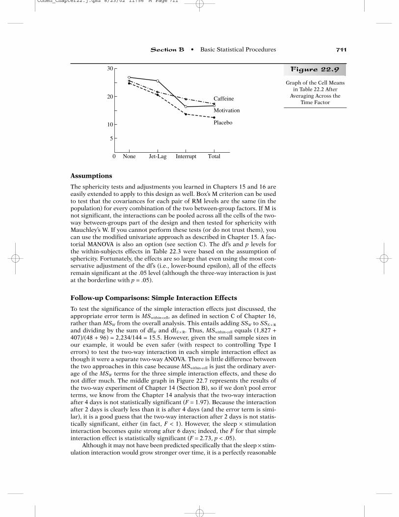
In Figure 22.9, I have graphed the sleep by stimulation interaction, byaveraging the three panels of Figure 22.7. Although the interaction looks likeit might be significant, we know from Table 22.3 that it is not. Rememberthat the error term for testing this interaction is based on subject-to-subjectvariability within each cell and does not benefit from the added power ofrepeated measures. The other two interactions use MSS × RM as their errorterm and therefore do gain the extra power usually conferred by repeatedmeasures. Of course, even if the sleep by stimulation interaction were sig-nificant, its interpretation would be qualified by the significance of thethree-way interaction. The significant three-way interaction tells us to becautious in our interpretation of the other six F ratios and suggests that welook at simple interaction effects.

There are three ways to look at simple interaction effects in a three-wayANOVA (depending on which factor is looked at one level at a time), but themost interesting two-way interaction for the present example is sleep depri-vation by stimulation, so we will look at that interaction at each level of thetime factor. The results have already been graphed this way in Figure 22.7. Itis easy to see that the three-way interaction in this study is due to the pro-gressive increase in the sleep by stimulation interaction over time.

MSA × B × R��

MSS × R

MSB × R�MSS × R

MSA × R�MSS × R

MSR�MSS × R

MSA × B�

MSW

MSB�MSW

MSA�MSW



Assumptions

The sphericity tests and adjustments you learned in Chapters 15 and 16 areeasily extended to apply to this design as well. Box’s M criterion can be usedto test that the covariances for each pair of RM levels are the same (in thepopulation) for every combination of the two between-group factors. If M isnot significant, the interactions can be pooled across all the cells of the two-way between-groups part of the design and then tested for sphericity withMauchley’s W. If you cannot perform these tests (or do not trust them), youcan use the modified univariate approach as described in Chapter 15. A fac-torial MANOVA is also an option (see section C). The df’s and p levels for the within-subjects effects in Table 22.3 were based on the assumption ofsphericity. Fortunately, the effects are so large that even using the most con-servative adjustment of the df’s (i.e., lower-bound epsilon), all of the effectsremain significant at the .05 level (although the three-way interaction is justat the borderline with p = .05).

Follow-up Comparisons: Simple Interaction Effects

To test the significance of the simple interaction effects just discussed, theappropriate error term is MSwithin-cell, as defined in section C of Chapter 16,rather than MSW from the overall analysis. This entails adding SSW to SSS × R

and dividing by the sum of dfW and dfS × R. Thus, MSwithin-cell equals (1,827 +407)/(48 + 96) = 2,234/144 = 15.5. However, given the small sample sizes inour example, it would be even safer (with respect to controlling Type Ierrors) to test the two-way interaction in each simple interaction effect asthough it were a separate two-way ANOVA. There is little difference betweenthe two approaches in this case because MSwithin-cell is just the ordinary aver-age of the MSW terms for the three simple interaction effects, and these donot differ much. The middle graph in Figure 22.7 represents the results ofthe two-way experiment of Chapter 14 (Section B), so if we don’t pool errorterms, we know from the Chapter 14 analysis that the two-way interactionafter 4 days is not statistically significant (F = 1.97). Because the interactionafter 2 days is clearly less than it is after 4 days (and the error term is simi-lar), it is a good guess that the two-way interaction after 2 days is not statis-tically significant, either (in fact, F < 1). However, the sleep × stimulationinteraction becomes quite strong after 6 days; indeed, the F for that simpleinteraction effect is statistically significant (F = 2.73, p < .05).

Although it may not have been predicted specifically that the sleep × stim-ulation interaction would grow stronger over time, it is a perfectly reasonable


Figure 22.9

20

30

10

5


Placebo

Caffeine

Motivation

Graph of the Cell Meansin Table 22.2 After

Averaging Across theTime Factor


result, and it would make sense to focus our remaining follow-up analyses onDay 6 alone. We would then be dealing with an ordinary 4 × 3 ANOVA with norepeated measures, and post hoc analyses would proceed by testing simplemain effects or interaction contrasts exactly as described in Chapter 14, Sec-tion C. Alternatively, we could have explored the significant three-way inter-action by testing the sleep by time interaction for each stimulation level or thestimulation by time interaction for each sleep deprivation level. In these twocases, the appropriate error term, if all of the assumptions of the overallanalysis are met, is MSS × RM from the omnibus analysis. However, as you knowby now, caution is recommended with respect to the sphericity assumption,which dictates that each simple interaction effect be analyzed as a separatetwo-way ANOVA in which only the interaction is analyzed.

Follow-up Comparisons: Partial Interactions

As in the case of the two-way ANOVA, a three-way ANOVA in which at leasttwo of the factors have three levels or more can be analyzed in terms of partialinteractions, either as planned comparisons or as a way to follow up a signif-icant three-way interaction. However, with three factors in the design, thereare two distinct options. The first type of partial interaction involves forminga pairwise or complex comparison for one of the factors and crosses that com-parison with all levels of the other two factors. For instance, you could reducethe stimulation factor to a comparison of caffeine and reward (pairwise) or toa comparison of placebo with the average of caffeine and reward (complex)but include all the levels of the other two factors. The second type of partialinteraction involves forming a comparison for two of the factors. For example,caffeine versus reward and jet lag versus interrupted crossed with the threetime periods. If a pairwise or complex comparison is created for all three fac-tors, the result is a 2 × 2 × 2 subset of the original design, which has only onenumerator df and therefore qualifies as an interaction contrast. A significantpartial interaction may be decomposed into a series of interaction contrasts,or one can plan to test several of these from the outset. Another alternative isthat a significant three-way interaction can be followed directly by post hocinteraction contrasts, skipping the analysis of partial interactions, even whenthey are possible. A significant three-way (i.e., 2 × 2 × 2) interaction contrastwould be followed by a test of simple interaction effects, and, if appropriate,simple main effects (i.e., t tests between two cells).

Follow-Up Comparisons: Three-Way Interaction Not Significant

When the three-way interaction is not significant, attention shifts to thethree two-way interactions. If none of the two-way interactions is signifi-cant, any significant main effect with more than two levels can be exploredfurther with pairwise or complex comparisons among its levels. If only oneof the two-way interactions is significant, the factor not involved in the inter-action can be explored in the usual way if its main effect is significant. Anysignificant two-way interaction can be followed up with an analysis of itssimple effects or with partial interactions and/or interaction contrasts, asdescribed in Chapter 14, Section C.

Planned Comparisons for the Three-Way ANOVA

Bear in mind that a three-way ANOVA with several levels of each factor cre-ates so many possibilities for post hoc testing that it is rare for a researcher



to follow every significant omnibus F ratio (remember, there are seven ofthese) with post hoc tests and every significant post hoc test with more local-ized tests until all allowable cell-to-cell comparisons are made. It is morecommon when analyzing a three-way ANOVA to plan several comparisonsbased on one’s research hypotheses.

Although a set of orthogonal contrasts is desirable, more often theplanned comparisons are a mixture of simple effects, two- and three-wayinteraction contrasts, and cell-to-cell comparisons. If there are not too manyof these, it is not unusual to test each planned comparison at the .05 level.However, if the planned comparisons are not orthogonal, and overlap in var-ious ways, the cautious researcher is likely to use the Bonferroni adjustmentto determine the alpha for each comparison. After the planned comparisonshave been tested, it is not unusual for a researcher to test the seven F ratiosof the overall analysis but to report and follow up only those effects that areboth significant and interesting (and whose patterns of means make sense).

When the RM Factor Has Only Two Levels

If you have only one RM factor in your three-way ANOVA, and that factor hasonly two levels, you have the option of creating difference scores (i.e., the dif-ference between the two RM levels) and conducting a two-way ANOVA on thedifference scores. For this two-way ANOVA, the main effect of factor A isreally the interaction of the RM factor with factor A, and similarly for factorB. The A × B interaction is really the three-way interaction of A, B, and theRM factor. The parts of the three-way ANOVA that you lose with this trick arethe three main effects and the A × B interaction, but if you are only interestedin interactions involving the RM factor, this shortcut can be convenient. Themost likely case in which you would want to use difference scores is when thetwo levels of the RM factor are measurements taken before and after sometreatment. However, as I mentioned in Chapter 16, this type of design is agood candidate for ANCOVA (you would use factorial ANCOVA if you hadtwo between-group factors).

Published Results of a Three-way ANOVA (One RM Factor)

It is not hard to find published examples of the three-way ANOVA with oneRM factor; the 2 × 2 × 2 design is probably the most common and is illus-trated in a study entitled “Outcome of Cognitive-Behavioral Therapy forDepression: Relation to Hemispheric Dominance for Verbal Processing”(Bruder, et al., 1997). In this experiment, two dichotic listening tasks wereused to assess hemispheric dominance: a verbal (i.e., syllables) task forwhich most people show a right-ear advantage (indicating left-hemisphericcerebral dominance for speech) and a nonverbal (i.e., complex tones) taskfor which most subjects exhibit a left-ear advantage. These two tasks are thelevels of the RM factor. The dependent variable was a measure of perceptualasymmetry (PA), based on how much more material is reported from theright ear as compared to the left ear. Obviously, a strong main effect of theRM factor is to be expected.

All of the subjects were patients with depression. The two between-groups factors were treatment group (cognitive therapy or placebo) andtherapy response or outcome (significant clinical improvement or not). Theexperiment tested whether people who have greater left-hemisphere domi-nance are more likely to respond to cognitive therapy; this effect is notexpected for those “responding” to a placebo. The results exhibited a clearpattern, as I have shown in Figure 22.10 (I redrew their figure to make the



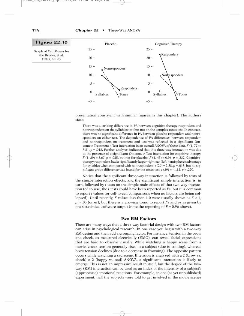
presentation consistent with similar figures in this chapter). The authorsstate:

There was a striking difference in PA between cognitive-therapy responders andnonresponders on the syllables test but not on the complex tones test. In contrast,there was no significant difference in PA between placebo responders and nonre-sponders on either test. The dependence of PA differences between respondersand nonresponders on treatment and test was reflected in a significant Out-come × Treatment × Test interaction in an overall ANOVA of these data, F (1, 72) =5.81, p = .018. Further analyses indicated that this three-way interaction was dueto the presence of a significant Outcome × Test interaction for cognitive therapy,F (1, 29) = 5.67, p = .025, but not for placebo, F (1, 43) = 0.96, p = .332. Cognitive-therapy responders had a significantly larger right-ear (left-hemisphere) advantagefor syllables when compared with nonresponders, t (29) = 2.58, p = .015, but no sig-nificant group difference was found for the tones test, t (29) = −1.12, p = .270.

Notice that the significant three-way interaction is followed by tests ofthe simple interaction effects, and the significant simple interaction is, inturn, followed by t tests on the simple main effects of that two-way interac-tion (of course, the t tests could have been reported as Fs, but it is commonto report t values for cell-to-cell comparisons when no factors are being col-lapsed). Until recently, F values less than 1.0 were usually shown as F < 1, p > .05 (or ns), but there is a growing trend to report Fs and ps as given byone’s statistical software output (note the reporting of F = 0.96 above).

Two RM FactorsThere are many ways that a three-way factorial design with two RM factorscan arise in psychological research. In one case you begin with a two-wayRM design and then add a grouping factor. For instance, tension in the browand cheek, as measured electrically (EMG), can reveal facial expressionsthat are hard to observe visually. While watching a happy scene from amovie, cheek tension generally rises in a subject (due to smiling), whereasbrow tension declines (due to a decrease in frowning). The opposite patternoccurs while watching a sad scene. If tension is analyzed with a 2 (brow vs.cheek) × 2 (happy vs. sad) ANOVA, a significant interaction is likely toemerge. This is not an impressive result in itself, but the degree of the two-way (RM) interaction can be used as an index of the intensity of a subject’s(appropriate) emotional reactions. For example, in one (as yet unpublished)experiment, half the subjects were told to get involved in the movie scenes


20

25

10

15

5

0

–5

Syllables Tones

Nonresponders

Placebo

Responders

20

25

10

15

5

0

–5

Syllables Tones

NonrespondersNonresponders

Cognitive Therapy

RespondersGraph of Cell Means for

the Bruder, et al. (1997) Study

Figure 22.10


they were watching, whereas the other half were told to analyze the scene forvarious technical details. As expected, the two-way interaction was strongerfor the involved subjects, producing a three-way interaction. In anotherexperiment subjects were selected from an introductory psychology classbased on their responses to an empathy questionnaire. Not surprisingly,there was again a three-way interaction due to the stronger two-way inter-action for the high-empathy as compared to the low-empathy subjects.

The example I will use to illustrate the calculation of a three-wayANOVA with two RM factors was inspired by a published study in industrialpsychology entitled: “Gender and attractiveness biases in hiring decisions:Are more experienced managers less biased?” (Marlowe, Schneider & Nel-son, 1996). For pedagogical reasons, I changed the structure and conclu-sions of the experiment quite a bit.

In my example the subjects are all men who are chosen for having a cor-porate position in which they are frequently making hiring decisions. Thebetween-groups factor is based on how many years of experience a subjecthas in such a position: little experience (less than 5 years), moderate experi-ence (5 to 10 years), or much experience (more than 10 years). The depend-ent variable is the rating a subject gives to each resume (with attachedphotograph) he is shown; low ratings indicate that the subject would not belikely to hire the applicant (0 = no chance), whereas high ratings indicate thathiring would be likely (9 = would certainly hire). The two RM factors are thegender of the applicant and his or her attractiveness, as based on prior rat-ings of the photographs (above-average, average, below average). Each sub-ject rates five applicants in each of the six attractiveness/gender categories;for each subject and each category, the five ratings have been averagedtogether and presented in Table 22.4. To reduce the necessary calculations Ihave included only four subjects in each experience group. Of course, the 30applicants rated by each subject would be mixed randomly for each subject,eliminating both the possibility of simple order effects and the need for coun-terbalancing. In addition, the resumes would be counterbalanced with thephotographs, so no photograph would be consistently paired with a betterresume (the resumes would be similar anyway).

For the sake of writing general formulas in which it is easy to spot thebetween-group and RM factors, I will use the letter A to represent thebetween-groups factor (amount of hiring experience, in this example) and Qand R to represent the two RM factors (gender and attractiveness, respec-tively). The “subject” factor will be designated as S. You have seen this factorbefore written as “between-subjects,” “sub” or “S,” but with two RM factorsthe shorter abbreviation is more convenient. The ANOVA that follows is themost complex one that will be described in this text. It requires all of the SScomponents of the previous analysis plus two more SS components that areextracted to create additional error terms.

The analysis can begin in the same way as the previous one—with thecalculation of SStotal and the SSs for the three main effects. The total numberof observations, NT, equals aqrn = 3 � 2 � 3 � 4 = 72. SStotal, as usual, is equal tothe biased variance of all 72 observations times 72, which equals 69.85. SSA

is based on the means of the three independent groups, which appear in theRow Means column, in the rows that represent cell means (i.e., each groupmean is the mean of the six RM cell means). SSR is based on the means forthe attractiveness levels, which appear in the Column Means row under thecolumns labeled “Mean” (which takes the mean across gender). The gendermeans needed for SSQ are not in the table but can be found by averaging sep-arately the column means for females and for males. The SSs for the maineffects can now be found in the usual way.



BE

LO

WA

VE

RA

GE

AB

OV

ER

ow

Fem

ale

Mal

eM

ean

Fem

ale

Mal

eM

ean

Fem

ale

Mal

eM

ean

Mea

ns

5.2

5.2

5.2

5.8

6.0

5.9

7.4

7.6

7.5

6.2

Low

5.8

6.0

5.9

6.4

5.2

5.8

7.6

8.0

7.8

6.5

5.6

5.6

5.6

6.0

6.2

6.1

6.6

7.8

7.2

6.3

4.4

5.8

5.1

7.0

6.8

6.9

7.8

6.4

7.1

6.37

Cel

l Mea

n5.

255.

655.

456.

36.

056.

175

7.35

7.45

7.4

6.34

17

4.8

5.4

5.1

5.6

6.0

5.8

6.4

7.0

6.7

5.87

Mod

erat

e5.

44.

85.

15.

46.

66.

05.

87.

66.

75.

934.

25.

24.

75.

05.

85.

47.

66.

87.

25.

774.

66.

05.

36.

25.

45.

87.

26.

46.

85.

97C

ell M

ean

4.75

5.35

5.05

5.55

5.95

5.75

6.75

6.95

6.85

5.88

33

4.4

5.8

5.1

6.0

7.0

6.5

7.0

5.6

6.3

5.97

Hig

h5.

26.

65.

95.

66.

25.

96.

64.

85.

75.

833.

66.

45.

06.

27.

87.

05.

26.

45.

85.

934.

05.

04.

55.

26.

86.

06.

85.

86.

35.

60C

ell M

ean

4.30

5.95

5.12

55.

756.

956.

356.

405.

656.

025

5.83

33C

ol M

ean

4.77

5.65

5.21

5.87

6.32

6.09

56.

836.

686.

755

6.02

Ta

ble

22.4


SSA = 72 � σ2(6.3417, 5.8833, 5.8333) = 3.77SSQ = 72 � σ2(5.8233, 6.2167) = 2.785SSR = 72 � σ2(5.21, 6.095, 6.755) = 28.85

As in the previous analysis we will need SSbetween-subjects based on the 12overall subject means (across all six categories of applicants). These are therow means (ignoring the rows labeled “Cell Means” and “Column Means,” ofcourse) in Table 22.4.

SSbet-S = 72 � σ2(6.2, 6.5, 6.3, 6.37, 5.87, 5.93, 5.77, 5.97, 5.97, 5.83, 5.93, 5.6)= 4.694 = SSS

Because this is the same SS you would get if you were going to calculate amain effect of subjects, I will call this SS component SSS.

Before we get enmeshed in the complexities of dealing with two RM fac-tors, we can complete the between-groups part of the analysis. I will use For-mula 16.2 from the two-way mixed design with an appropriate change in thesubscripts:

SSW = SSS − SSA Formula 22.8

For this example, SSW = 4.694 − 3.77 = .924

dfA = a − 1 = 3 − 1 = 2dfW = a(n − 1) = an − a = 12 − 3 = 9

Therefore,

MSA = = = 1.885 and

MSW = = = .103

Finally,

FA = = 18.4

The appropriate critical F is F.05(2,9) = 4.26, so FA is easily significant. Alook at the means for the three groups of subjects shows us that managerswith greater experience are, in general, more cautious with their hirabilityratings (perhaps they have been “burned” more times), especially when com-paring low to moderate experience. However, there is no point in trying tointerpret this finding before testing the various interactions, which maymake this finding irrelevant or even misleading. I have completed thebetween-groups part of the analysis at this point just to show you that atleast part of the analysis is easy and to get it out of the way before the morecomplicated within-subject part of the analysis begins.

With only one RM factor there is only one error term that involves aninteraction with the subject factor, and that error term is found easily bysubtraction. However, with two RM factors the subject factor interacts witheach RM factor separately, and with the interaction of the two of them, yield-ing three different error terms. The extraction of these extra error termsrequires the collapsing of more intermediate tables, and the calculation ofmore intermediate SS terms. Of course, the calculations are performed thesame way as always—there are just more of them. Let’s begin, however, withthe numerators of the various interaction terms, which involve the sameprocedures as the three-way analysis with only one RM factor. First, we can

1.885�.103

.924�

9SSW�

9

3.77�

2SSA�

2



get SSAQR from the 18 cell means in Table 22.4 (all of the female and malecolumns of the three Cell Means rows).

SSAQR = 72 � σ2(cell means) = 72 � .694 = 49.96

The means needed to find SSAR are averaged across the Q factor (i.e.,gender); they are found in the three Cell Mean rows, in the columns labeled“Means.”

SSAR = 72 � σ2(5.45, 6.175, 7.4, 5.05, 5.75, 6.85, 5.125, 6.35, 6.025) = 72 � .5407 = 38.93

The means for SSQR are the Column Means in Table 22.4 for females and males(but not Means) and are averaged across all subjects, regardless of group.

SSQR = 72 � σ2(4.77, 5.65, 5.87, 6.32, 6.83, 6.68) = 72 � .4839 = 34.84

The means needed for SSAQ do not have a convenient place in Table 22.4;those means would fit easily in a table in which the female columns are alladjacent (for Below, Average, and Above), followed by the three malecolumns. Using Table 22.4, you can average together for each group all of thefemale cell means and then all of the male cell means, thus producing the sixAQ means.

SSAQ = 72 � σ2(6.3, 6.383, 5.683, 6.083, 5.483, 6.185) = 72 � .1072 = 7.72

Now we can get the SSs for all of the interactions by subtraction, using For-mula 22.1 (except that B and C have been changed to Q and R):

SSA × Q = SSAQ − SSA − SSQ = 7.72 − 3.77 − 2.785 = 1.16SSA × R = SSAR − SSA − SSR = 38.93 − 3.77 − 28.85 = 6.31SSQ × R = SSQR − SSQ − SSR = 34.84 − 2.785 − 28.85 = 3.21

SSA × Q × R = SSAQR − SSA × Q − SSA × R − SSQ × R − SSA − SSQ − SSR

= 49.96 − 1.16 − 6.31 − 3.21 − 3.77 − 2.785 − 28.85 = 3.875

The next (and trickiest) step is to calculate the SSs for the three RMerror terms. These are the same error terms I described at the end of SectionA in the context of the two-way RM ANOVA. For each RM factor the appro-priate error term is based on the interaction of the subject factor with thatRM factor. The more that subjects move in parallel from one level of the RMfactor to another, the smaller the error term. The error term for each RM fac-tor is based on averaging over the other factor. However, the third RM errorterm, the error term for the interaction of the two RM factors, is based onthe three-way interaction of the subject factor and the two RM factors, withno averaging of scores. To the extent that each subject exhibits the same two-way interaction for the RM factors, this error term will be small.

Two more intermediate SSs are required: SSQS, and SSRS. These SSscome from two additional two-way means tables, each one averaging scoresover one of the RM factors but not the other. (Note: The A factor isn’t men-tioned for these components because it is simply being ignored. Some of thesubject means are from subjects in the same group, and some are from sub-jects in different groups, but this distinction plays no role for these SS com-ponents.) You can get SSRS from the entries in the columns labeled “Means”(ignoring the rows labeled “Cell Means” and “Column Means,” of course) inTable 22.4; in all there are 36 male/female averages, or RS means:

SSRS = 72 � σ2(RS means) = 72 � .6543 = 47.11

To find the QS means, you need to create, in addition to the row means inTable 22.4, two additional means for each row: one for the “females” in thatrow, and one for the “males,” for a total of 24 “gender” row means.



SSQS = 72 � σ2(6.13, 6.27, 6.6, 6.4, 6.07, 6.53, 6.4, 6.33, 5.6, 6.13, 5.53, 6.33, 5.6, 5.93, 6, 5.93, 5.8, 6.13, 5.8, 5.87, 5.0, 6.87, 5.33, 5.87)

= 72 � .1737 = 12.51

(Note: the means are in the order “female, male” for each subject (i.e.,row)—top to bottom—of Table 22.4.)

Now we are ready to get the error terms by subtraction, using Formula22.9A.

SSQ × S = SSQS − SSQ − SSS − SSA × Q Formula 22.9A

So,

SSQ × S = 12.51 − 2.785 − 4.694 − 1.16 = 3.87

[Note: I subtracted the group by gender interaction at the end of the pre-ceding calculation because what we really want (and what I mean bySSQ × S) is the gender by subject interaction within each group (i.e., level ofthe A factor), added across all the groups. This is not the same as just find-ing the gender by subject interaction, ignoring group. Any group by gen-der interaction will increase the gender by subject interaction whenignoring group, but not if you calculate the interaction separately withineach group. Rather than calculating the gender by subject interaction foreach group, it is easier to calculate the overall interaction ignoring groupand then subtract the group by gender interaction. The same trick is usedto find SSR × S.]

SSR × S = SSRS − SSR − SSS − SSA × R Formula 22.9B

Therefore,

SSR × S = 47.11 − 28.85 − 4.694 − 6.31 = 7.26

Finally, the last error term, SSQ × R × S, can be found by subtracting all ofthe other SS components from SStotal. To simplify this last calculation, notethat SStotal is the sum of all the cell-to-cell variation and the four errorterms:

SStotal = SSAQR + SSW + SSQ × S + SSR × S + SSQ × R × S Formula 22.9C

So,

SSQ × R × S = SStotal − SSAQR − SSW − SSQ × S − SSR × S

= 69.85 − 49.96 − .924 − 3.87 − 7.26 = 7.836

The degrees of freedom are divided up for this design in a way that isbest illustrated in a df tree, as shown in Figure 22.11. The formulas for thedf’s are as follows:

a. dfA = a − 1 Formula 22.10b. dfQ = q − 1c. dfR = r − 1d. dfA × Q = (a − 1)(q − 1)e. dfA × R = (a − 1)(r − 1)f. dfQ × R = (q − 1)(r − 1)g. dfA × Q × R = (a − 1)(q − 1)(r − 1)h. dfW = a (n − 1)i. dfQ × S = dfQ � dfW = a(q − 1)(n − 1)j. dfR × S = dfR � dfW = a(r − 1)(n − 1)k. dfQ × R × S = dfQ � dfR � dfW = a(q − 1)(r − 1)(n − 1)

For this example,



dfA = 3 − 1 = 2

dfQ = 2 − 1 = 1

dfR = 3 − 1 = 2

dfA × Q = 2 � 1 = 2

dfA × R = 2 � 2 = 4

dfQ × R = 1 � 2 = 2

dfA × Q × R = 2 � 1 � 2 = 4

dfW = 3 � 3 = 9

dfQ × S = dfQ � dfW = 1 � 9 = 9

dfR × S = dfR � dfW = 2 � 9 = 18

dfQ × R × S = dfQ � dfR � dfW = 1 � 2 � 9 = 18

Note that the sum of all the df’s is 71, which equals dftotal (NT − 1 = aqrn − 1 =72 − 1). When you have converted each SS to an MS, the seven F ratios areformed as follows:


df total[aqrn–1]

df A[a–1]

df W[a(n–1)]

df between-S

[an–1]

df AXQ[(a–1)(q–1)]

df QXR[(q–1)(r–1)]

df Q[q–1]

df QXS[a(n–1)(q–1)]

df R[r–1] df RXS

[a(n–1)(r–1)]

df AXR[(a–1)(r–1)]

df QXRXS[a(n–1)(q–1)(r–1)]

df AXQXR[(a–1)(q–1)(r–1)]

df within-S[an(qr–1)]

Degrees of Freedom Treefor 3-Way ANOVA withRepeated Measures on

Two Factors

Figure 22.11

a. FA =

b. FQ =

c. FR =

d. FA × Q =

e. FA × R =

f. FQ × R =

g. FA × Q × R =MSA × Q × R��MSQ × R × S

MSQ × R��MSQ × R × S

MSA × R�MSR × S

MSA × Q�MSQ × S

MSR�MSR × S

MSQ�MSQ × S

MSA�MSW

Formula 22.11

The completed analysis is shown in Table 22.5. Notice that each of thethree different RM error terms is being used twice. This is just an extension


of what you saw in the two-way mixed design when the S × RM error termwas used for both the RM main effect and its interaction with the between-groups factor.

Interpreting the Results

Although the three-way interaction was not significant, you will probablywant to graph all of the cell means in any case to see what’s going on in yourresults; I did this in Figure 22.12, choosing applicant gender as the variablewhose levels are represented by different graphs and hiring experience levelsto be represented as different lines on each graph. You can see by comparingthe two graphs in the figure why the F ratio for the three-way interactionwas not very small, even though it failed to attain significance. The three-way interaction is due almost entirely to the drop in hirability from averageto above average attractiveness only for highly experienced subjects judgingmale applicants. It is also obvious (and not misleading) that the main effectof attractiveness should be significant (with the one exception just men-tioned, all the lines go up with increasing attractiveness), and the main effectof gender as well (the lines on the “male” graph are generally higher.) That


Source SS df MS F p

Between-groups 4.694 11Hiring Experience 3.77 2 1.885 18.4 <.001Within-group error .924 9 .103

Within-subjects 65.156 60Gender 2.785 1 2.785 6.48 <.05Group × Gender 1.16 2 .580 1.35 >.05Gender × Subject 3.87 9 .430

Attractiveness 28.85 2 14.43 35.81 <.001Group × Atttract 6.31 4 1.578 3.92 <.05Attract × Subject 7.26 18 .403

Gender × Attract 3.21 2 1.60 3.69 <.05Group × Gender × Attract 3.875 4 .970 2.23 >.05Gender × Attract × Subject 7.836 18 .435

Note: The note from Table 22.3 applies here as well.

Table 22.5

Figure 22.12

7

6

5

0Below AboveAverage

Low

Female

Moderate

High

7

6

5

0Below AboveAverage

LowMale

Moderate

High

Graph of the Cell Meansfor the Data in Table 22.4


the line for the low experience group is consistently above the line for mod-erate experience seems to account, at least in part, for the significance of themain effect for that factor.

The significant attractiveness by experience (i.e., group) interaction isclearly due to a strong interaction for the male condition being averagedwith a lack of interaction for the females (Figure 22.13 shows the male andfemale conditions averaged together, which bears a greater resemblance tothe male than female condition). This is a case when a three-way interactionthat is not significant should nonetheless lead to caution in interpreting sig-nificant two-way interactions.

Perhaps, the most interesting significant result is the interaction ofattractiveness and gender. Figure 22.14 shows that although attractiveness isa strong factor in hirability for both genders, it makes somewhat less of adifference for males. However, the most potentially interesting result wouldhave been the three-way interaction, had it been significant; it could haveshown that the impact of attractiveness on hirability changes with the expe-rience of the employer, but more for male than female applicants.


7

6

5

0Below AboveAverage

Low

Average of Female andMale Applicants

Moderate

High

Graph of the Cell Meansfor Table 22.4 After

Averaging Across Gender

Figure 22.13

7

6

5

0Below AboveAverage

Average of the ThreeHiring Experience Levels

FemaleMale

Graph of the Cell Meansfor Table 22.4 After

Averaging Across theLevels of Hiring

Experience

Figure 22.14


Assumptions

For each of the three RM error terms (Q × S, R × S, Q × R × S), pairwise inter-actions should be the same for each independent group; these assumptionscan be tested with three applications of Box’s M test. With interactionspooled across groups, sphericity can then be tested with Mauchly’s W foreach of the three error terms (Huynh & Mandeville, 1979). In the precedingexample, sphericity is not an issue for gender, which has only two levels, butsphericity can be tested separately for both attractiveness and the gender byattractiveness interaction. However, rather than relying on the outcome ofstatistical tests of assumptions, researchers often “play it safe” by ensuringthat all of the groups have the same number of subjects and adjusting the dfwith epsilon before testing effects involving a repeated-measures factor.

Follow-Up Comparisons

Given the significance of the attractiveness by experience interaction, itwould be reasonable to perform follow-up tests, similar to those describedfor the two-way mixed design in Chapter 16. This includes the possibility ofanalyzing simple effects (a one-way ANOVA at each attractiveness level or aone-way RM ANOVA for each experience group), partial interactions (e.g.,averaging the low and moderate experience conditions and performing theresulting 2 × 3 ANOVA) or interaction contrasts (e.g., the average of the lowand moderate conditions and the high condition crossed with the averageand above average attractiveness conditions). Such tests, if significant, couldjustify various cell-to-cell comparisons. To follow up on the significant gen-der by attractiveness interaction, the most sensible approach would be sim-ply to conduct RM t tests between the genders at each level of attractiveness.

In general, planned and post hoc comparisons for the three-way ANOVAwith two RM factors follow the same logic as those described for the designwith one RM factor. The only differences concern the error terms for thesecomparisons. If your between-group factor is significant, involves more thantwo levels, and is not involved in an interaction with one of the RM factors,you can use MSW from the overall analysis as your error term. For all othercomparisons, using an error term from the overall analysis requires somequestionable homogeneity assumption. For tests involving one or both ofthe two RM factors, it is safest to perform all planned and post hoc compar-isons using an error term based only on the conditions included in the test.

Published Results of a Three-way ANOVA (Two RM Factors)

Banaji and Hardin (1996) studied automatic stereotyping by presentingcommon gender pronouns to subjects (e.g., she, him) and measuring theirreaction times to judging the gender of the pronouns (i.e., male or female; noneutral pronouns were used in their Experiment 1). The interesting manip-ulation was that the pronouns were preceded by primes—words that sub-jects were told to ignore but which could refer to a particular gender bydefinition (i.e., mother) or by stereotype (i.e., nurse). The gender of theprime on each trial was either female, male, neutral (i.e., postal clerk) or justa string of letters (nonword). The authors describe their 4 × 2 × 2 experi-mental design as a “mixed factorial, with subject gender the between-subjects factor” (p. 138). An excerpt of their results follows:

The omnibus Prime Gender (female, male, neutral, nonword) × Target Gender(female, male) × Subject Gender (female, male) three-way analysis of varianceyielded the predicted Prime Gender × Target Gender interaction, F (3,198) =



72.25, p < .0001 . . . No other reliable main effects or interactions were obtainedas a function of either subject gender or target gender (Fs < 1) (p. 138).

The significant two-way interaction was then followed with an interactioncontrast (dropping the neutral and nonword prime conditions) and cell-to-cell comparisons:

The specific Prime Gender × Target Gender interaction (excluding the neutralconditions) was also reliable, F (1,66) = 117.56, p < .0001. Subjects were faster tojudge male pronouns after male than female primes, t (67) = 11.59, p < .0001, butfaster to judge female pronouns after female than male primes, t (67) = 6.90, p <.0001 (p. 138).

1. The calculation of the three-way ANOVA with repeated measures on onefactor follows the basic outline of the independent three-way ANOVA, asdescribed in Section A, but adds elements of the mixed design, as delin-eated in Chapter 16. The between-subject factors are labeled A and B,whereas the within-subject factor is labeled R (short for RM). The num-ber of levels of the factors are symbolized by a, b, and c, respectively.The following steps should be followed:a. Begin with a table of the individual scores and then find the mean for

each level of each factor, the mean for each different subject (averag-ing across the levels of the RM factor), and the mean for each cell ofthe three-way design. From your table of cell means, create three“two-way” tables of means, in each case taking a simple average ofthe cell means across one of the three factors.

b. Use Formula 14.3 to find SStotal from the individual scores; SSA, SSB,and SSR from the means at each factor level; SSbetween-subjects from themeans for each subject; SSABR from the cell means; and SSAB, SSAR,and SSBR from the two-way tables of means.

c. Find the SS components for the three two-way interactions, thethree-way interaction, and the two error terms (SSW and SSS × R) bysubtraction. Divide these six SS components, along with the three SScomponents for the main effects, by their respective df to create thenine necessary MS terms.

d. Form the seven F ratios by using MSW as the error term for the maineffects of A and B and their interaction and then, using MSS × R as theerror term for the main effect of the RM factor, its interaction with A,its interaction with B, and the three-way interaction.

2. The calculation of the three-way ANOVA with repeated measures on twofactors is related to both the independent three-way ANOVA and thetwo-way RM ANOVA. The between-subject factor is labeled A, whereasthe two RM factors are labeled R and Q. The number of levels of the fac-tors are symbolized by a, r, and q, respectively. The following stepsshould be followed.a. Begin with a table of the individual scores and then find the mean for

each level of each factor, the mean for each different subject (averag-ing across the levels of both RM factors), and the mean for each cellof the three-way design. From your table of cell means, create three“two-way” tables of means, in each case taking a simple average ofthe cell means across one of the three factors. In addition, create twomore two-way tables in which scores are averaged over one RM fac-tor or the other, but not both, and subjects are not averaged acrossgroups (i.e., each table is a two-way matrix of subjects by one of theRM factors.).

b. Use Formula 14.3 to find SStotal from the individual scores; SSA, SSQ,and SSR from the means at each factor level; SSS from the means foreach subject; SSABR from the cell means; SSAB, SSAR, and SSBR from the


BSUMMARY


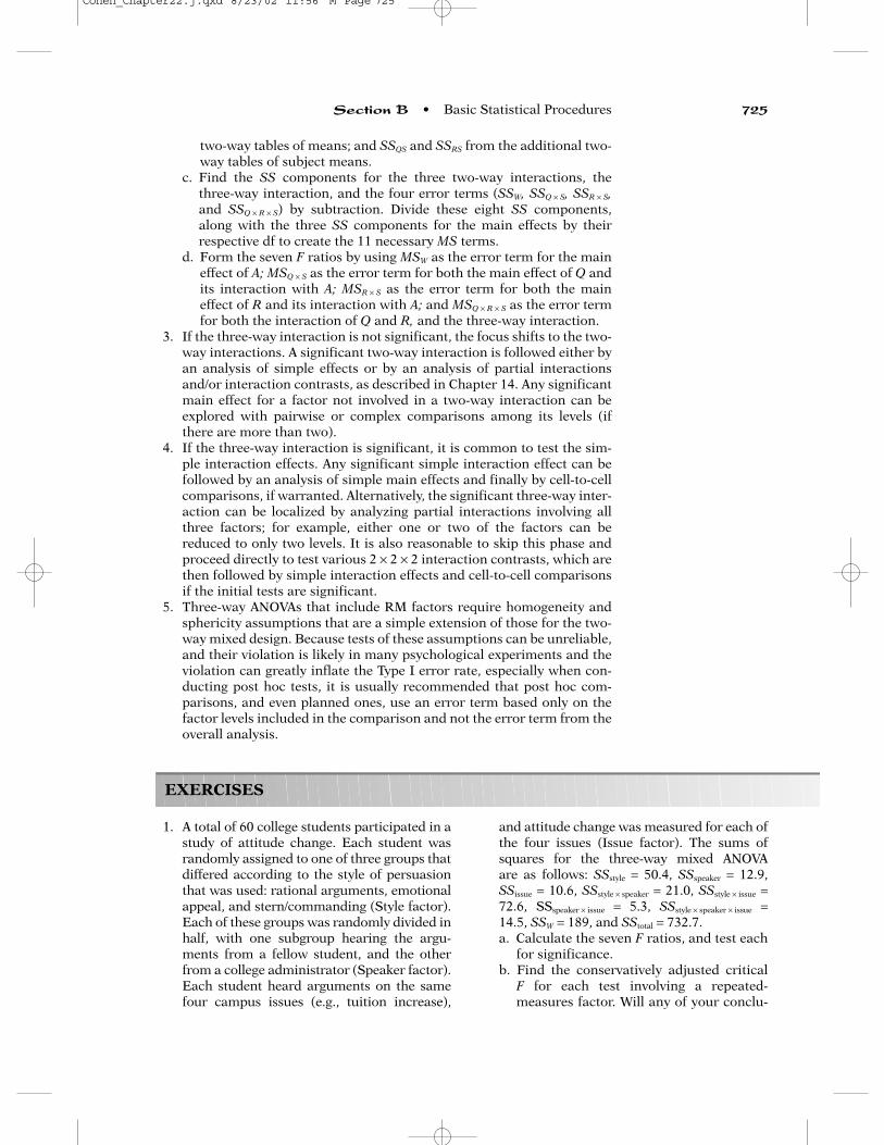
two-way tables of means; and SSQS and SSRS from the additional two-way tables of subject means.

c. Find the SS components for the three two-way interactions, thethree-way interaction, and the four error terms (SSW, SSQ × S, SSR × S,and SSQ × R × S) by subtraction. Divide these eight SS components,along with the three SS components for the main effects by theirrespective df to create the 11 necessary MS terms.

d. Form the seven F ratios by using MSW as the error term for the maineffect of A; MSQ × S as the error term for both the main effect of Q andits interaction with A; MSR × S as the error term for both the maineffect of R and its interaction with A; and MSQ × R × S as the error termfor both the interaction of Q and R, and the three-way interaction.

3. If the three-way interaction is not significant, the focus shifts to the two-way interactions. A significant two-way interaction is followed either byan analysis of simple effects or by an analysis of partial interactionsand/or interaction contrasts, as described in Chapter 14. Any significantmain effect for a factor not involved in a two-way interaction can beexplored with pairwise or complex comparisons among its levels (ifthere are more than two).

4. If the three-way interaction is significant, it is common to test the sim-ple interaction effects. Any significant simple interaction effect can befollowed by an analysis of simple main effects and finally by cell-to-cellcomparisons, if warranted. Alternatively, the significant three-way inter-action can be localized by analyzing partial interactions involving allthree factors; for example, either one or two of the factors can bereduced to only two levels. It is also reasonable to skip this phase andproceed directly to test various 2 × 2 × 2 interaction contrasts, which arethen followed by simple interaction effects and cell-to-cell comparisonsif the initial tests are significant.

5. Three-way ANOVAs that include RM factors require homogeneity andsphericity assumptions that are a simple extension of those for the two-way mixed design. Because tests of these assumptions can be unreliable,and their violation is likely in many psychological experiments and theviolation can greatly inflate the Type I error rate, especially when con-ducting post hoc tests, it is usually recommended that post hoc com-parisons, and even planned ones, use an error term based only on thefactor levels included in the comparison and not the error term from theoverall analysis.


EXERCISES

1. A total of 60 college students participated in astudy of attitude change. Each student wasrandomly assigned to one of three groups thatdiffered according to the style of persuasionthat was used: rational arguments, emotionalappeal, and stern/commanding (Style factor).Each of these groups was randomly divided inhalf, with one subgroup hearing the argu-ments from a fellow student, and the otherfrom a college administrator (Speaker factor).Each student heard arguments on the samefour campus issues (e.g., tuition increase),

and attitude change was measured for each ofthe four issues (Issue factor). The sums ofsquares for the three-way mixed ANOVA are as follows: SSstyle = 50.4, SSspeaker = 12.9,SSissue = 10.6, SSstyle × speaker = 21.0, SSstyle × issue =72.6, SSspeaker × issue = 5.3, SSstyle × speaker × issue =14.5, SSW = 189, and SStotal = 732.7.a. Calculate the seven F ratios, and test each

for significance.b. Find the conservatively adjusted critical

F for each test involving a repeated-measures factor. Will any of your conclu-



sions be affected if you do not make anyassumptions about sphericity?

2. Based on a questionnaire they had filled outearlier in the semester, students were classi-fied as high, low, or average in empathy. The12 students recruited in each category forthis experiment were randomly divided inhalf, with one subgroup given instructions towatch videotapes to check for the quality ofthe picture and sound (detail group) and theother subgroup given instructions to getinvolved in the story portrayed in the videotape. All subjects viewed the same twovideotapes (in counterbalanced order): onepresenting a happy story and one presentinga sad story. The dependent variable was thesubject’s rating of his or her mood at the endof each tape, using a 10-point happinessscale (0 = extremely sad, 5 = neutral, and 10 =extremely happy). The data for the studyappear in the following table:

a. Calculate the three-way mixed-designANOVA for the data. Present your resultsin a summary table.

b. Use graphs of the cell means to help youdescribe the pattern underlying eacheffect that was significant in part a.

c. Do you need to retest any of your resultsin part a if you make no assumptionsabout sphericity? Explain.

d. How can you transform the data above soit can be analyzed by a two-way independ-ent-groups ANOVA? Which effects fromthe analysis in part a would no longer betestable?

e. If a simple order effect is present in thedata, which error term is being inflated?How can you remove the extra variancefrom that error term?

3. The dean at a large college is testing theeffects of a new advisement system on stu-dents’ feelings of satisfaction with their edu-cational experience. A random sample of 12first-year students coming from small highschools was selected, along with an equal-sized sample of students from large highschools. Within each sample, a third of thestudents were randomly assigned to the newsystem, a third to the old system, and a thirdto a combination of the two systems. Satis-faction was measured on a 10-point scale (10 = completely satisfied) at the end of eachstudent’s first, second, third, and fourthyears. The data for the study appear in thefollowing table:

LOW AVERAGE HIGH

EMPATHY EMPATHY EMPATHYHappy Sad Happy Sad Happy Sad

Detail 6 5 5 4 7 36 5 7 2 8 35 7 5 3 7 17 4 5 5 5 54 6 4 4 6 46 5 5 5 5 5

Involved 5 4 6 2 7 25 4 6 2 8 16 4 7 1 9 14 5 4 4 7 25 3 6 2 6 14 5 4 4 7 2

SMALL HIGH SCHOOL LARGE HIGH SCHOOLFirst Second Third Fourth First Second Third Fourth

Old System 4 4 5 4 5 5 5 65 5 4 4 6 7 7 63 4 5 6 4 4 4 45 4 4 6 5 5 5 5

New System 6 5 6 7 7 8 8 87 8 9 9 7 8 8 85 4 4 5 6 7 7 76 6 7 7 6 5 6 8

Combined 5 5 6 6 9 7 7 74 5 6 7 8 7 7 66 6 5 6 9 6 5 55 6 6 6 8 6 6 8


a. Calculate the appropriate three-wayANOVA for the data. Present your resultsin a summary table.

b. Use graphs of the cell means to help youdescribe the pattern underlying each effectthat was significant in part a. Describe apartial interaction that would be meaning-ful. How might you use trend components?

c. What analyses of simple effects are justified,if any, by the results in part a? What errorterm should you use in each case if youmake no assumptions about sphericity?

d. Find the conservatively adjusted critical F for each test involving a repeated-measures factor. Will any of your conclu-sions be affected if you do not make anyassumptions about sphericity?

4. Imagine an experiment in which all subjectssolve two types of problems (spatial and ver-bal), each at three levels of difficulty (easy,moderate, and hard). Half of the 24 subjectsare given instructions to use visual imagery,and half are told to use subvocalization. Thedependent variable is the number of eyemovements that a subject makes during the5-second problem-solving period. The cellmeans for this experiment are given in thefollowing table:

a. Given that SStype × S = 224, SSdifficulty × S = 130,SStype × difficulty × S = 62, and SSW = 528, per-form the appropriate three-way ANOVAon the data. Present your results in a sum-mary table.

b. Graph the Type × Difficulty means, aver-aging across instruction group. Comparethis graph to the Type × Difficulty graphfor each instruction group. Can the over-all Type × Difficulty interaction be mean-ingfully interpreted? Explain.

c. Find the conservatively adjusted critical Ffor each test. Will any of your conclusionsbe affected if you do not assume thatsphericity exists in the population?

d. Given the results you found in part a,which simple effects can be justifiablyanalyzed?

5. Imagine that the psychologist in Exercise 6of Section A runs her study under two differ-ent conditions with two different randomsamples of subjects. The two conditionsdepend on the type of background musicplayed to the subjects as they memorize thelist of words: very happy or very sad. Thenumber of words recalled in each word cate-gory for each subject in the two groups isgiven in the following table:


SUBVOCAL IMAGERY

INSTRUCTIONS INSTRUCTIONSDifficulty Spatial Verbal Spatial Verbal

Easy 1.5 1.6 3.9 2.2Moderate 2.5 1.9 5.2 2.4Hard 2.7 2.1 7.8 2.8

SAD NEUTRAL HAPPYLow Medium High Low Medium High Low Medium High

Happy 4 6 9 3 5 6 4 4 9Music 2 5 7 4 6 7 5 6 6

4 7 5 3 5 5 4 5 72 5 4 4 6 6 4 4 54 8 8 5 7 7 5 5 103 5 6 5 5 6 6 4 5

Sad 5 6 9 2 4 6 3 4 6Music 3 5 9 3 6 5 4 5 5

6 7 6 2 4 5 3 3 63 6 7 3 4 6 4 4 54 10 9 4 6 7 5 5 85 5 7 4 5 6 4 4 5


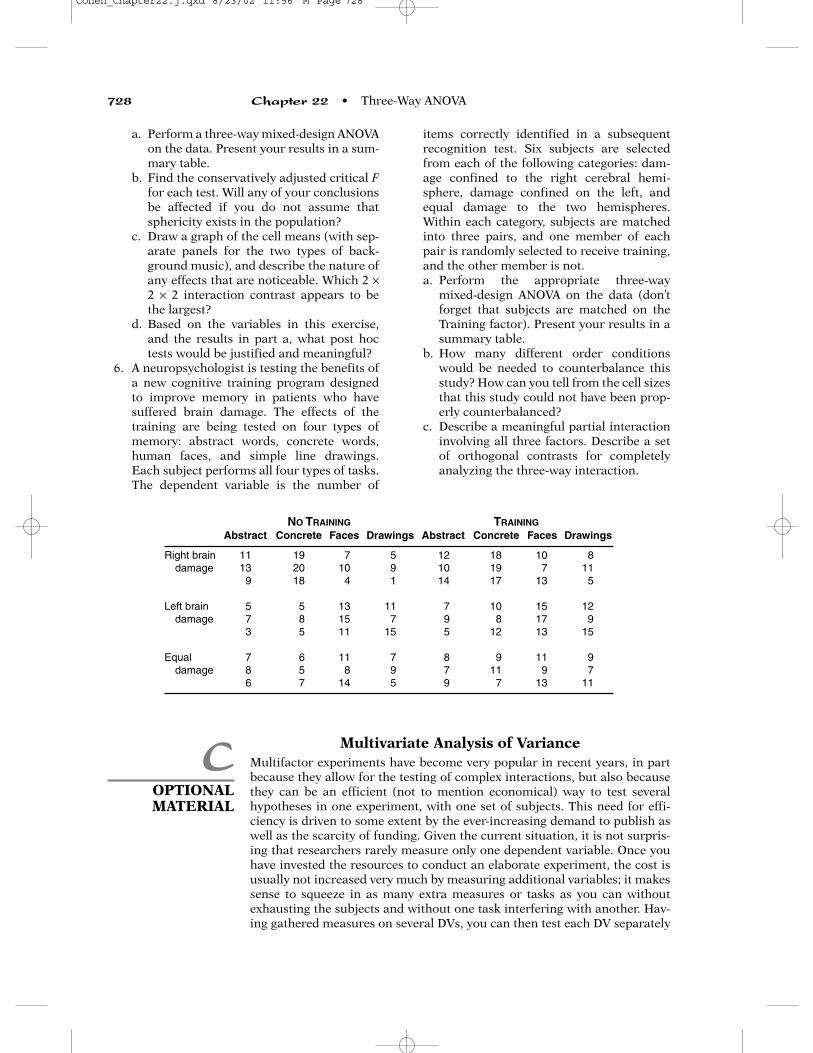
a. Perform a three-way mixed-design ANOVAon the data. Present your results in a sum-mary table.

b. Find the conservatively adjusted critical Ffor each test. Will any of your conclusionsbe affected if you do not assume thatsphericity exists in the population?

c. Draw a graph of the cell means (with sep-arate panels for the two types of back-ground music), and describe the nature ofany effects that are noticeable. Which 2 ×2 × 2 interaction contrast appears to bethe largest?

d. Based on the variables in this exercise,and the results in part a, what post hoctests would be justified and meaningful?

6. A neuropsychologist is testing the benefits ofa new cognitive training program designedto improve memory in patients who havesuffered brain damage. The effects of thetraining are being tested on four types ofmemory: abstract words, concrete words,human faces, and simple line drawings.Each subject performs all four types of tasks.The dependent variable is the number of

items correctly identified in a subsequentrecognition test. Six subjects are selectedfrom each of the following categories: dam-age confined to the right cerebral hemi-sphere, damage confined on the left, andequal damage to the two hemispheres.Within each category, subjects are matchedinto three pairs, and one member of eachpair is randomly selected to receive training,and the other member is not.a. Perform the appropriate three-way

mixed-design ANOVA on the data (don’tforget that subjects are matched on theTraining factor). Present your results in asummary table.

b. How many different order conditionswould be needed to counterbalance thisstudy? How can you tell from the cell sizesthat this study could not have been prop-erly counterbalanced?

c. Describe a meaningful partial interactioninvolving all three factors. Describe a setof orthogonal contrasts for completelyanalyzing the three-way interaction.


NO TRAINING TRAININGAbstract Concrete Faces Drawings Abstract Concrete Faces Drawings

Right brain 11 19 7 5 12 18 10 8damage 13 20 10 9 10 19 7 11

9 18 4 1 14 17 13 5

Left brain 5 5 13 11 7 10 15 12damage 7 8 15 7 9 8 17 9

3 5 11 15 5 12 13 15

Equal 7 6 11 7 8 9 11 9damage 8 5 8 9 7 11 9 7

6 7 14 5 9 7 13 11

COPTIONALMATERIAL

Multivariate Analysis of VarianceMultifactor experiments have become very popular in recent years, in partbecause they allow for the testing of complex interactions, but also becausethey can be an efficient (not to mention economical) way to test severalhypotheses in one experiment, with one set of subjects. This need for effi-ciency is driven to some extent by the ever-increasing demand to publish aswell as the scarcity of funding. Given the current situation, it is not surpris-ing that researchers rarely measure only one dependent variable. Once youhave invested the resources to conduct an elaborate experiment, the cost isusually not increased very much by measuring additional variables; it makessense to squeeze in as many extra measures or tasks as you can withoutexhausting the subjects and without one task interfering with another. Hav-ing gathered measures on several DVs, you can then test each DV separately


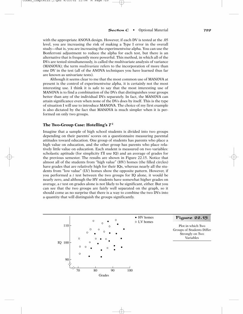
with the appropriate ANOVA design. However, if each DV is tested at the .05level, you are increasing the risk of making a Type I error in the overallstudy—that is, you are increasing the experimentwise alpha. You can use theBonferroni adjustment to reduce the alpha for each test, but there is analternative that is frequently more powerful. This method, in which all of theDVs are tested simultaneously, is called the multivariate analysis of variance(MANOVA); the term multivariate refers to the incorporation of more thanone DV in the test (all of the ANOVA techniques you have learned thus farare known as univariate tests).

Although it seems clear to me that the most common use of MANOVA atpresent is the control of experimentwise alpha, it is certainly not the mostinteresting use. I think it is safe to say that the most interesting use ofMANOVA is to find a combination of the DVs that distinguishes your groupsbetter than any of the individual DVs separately. In fact, the MANOVA canattain significance even when none of the DVs does by itself. This is the typeof situation I will use to introduce MANOVA. The choice of my first exampleis also dictated by the fact that MANOVA is much simpler when it is per-formed on only two groups.

The Two-Group Case: Hotelling’s T 2

Imagine that a sample of high school students is divided into two groupsdepending on their parents’ scores on a questionnaire measuring parentalattitudes toward education. One group of students has parents who place ahigh value on education, and the other group has parents who place rela-tively little value on education. Each student is measured on two variables:scholastic aptitude (for simplicity I’ll use IQ) and an average of grades forthe previous semester. The results are shown in Figure 22.15. Notice thatalmost all of the students from “high value” (HV) homes (the filled circles)have grades that are relatively high for their IQs, whereas nearly all the stu-dents from “low value” (LV) homes show the opposite pattern. However, ifyou performed a t test between the two groups for IQ alone, it would benearly zero, and although the HV students have somewhat higher grades onaverage, a t test on grades alone is not likely to be significant, either. But youcan see that the two groups are fairly well separated on the graph, so itshould come as no surprise that there is a way to combine the two DVs intoa quantity that will distinguish the groups significantly.

Section C • Optional Material 729

Figure 22.15

110

100IQ

90

70 90 10080Grades

HV homesLV homes

Plot in which TwoGroups of Students Differ

Strongly on TwoVariables


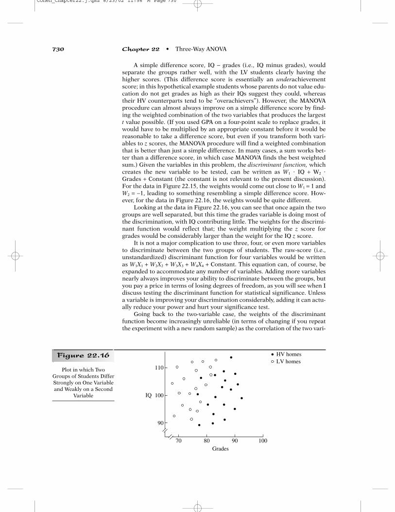
A simple difference score, IQ − grades (i.e., IQ minus grades), wouldseparate the groups rather well, with the LV students clearly having thehigher scores. (This difference score is essentially an underachievementscore; in this hypothetical example students whose parents do not value edu-cation do not get grades as high as their IQs suggest they could, whereastheir HV counterparts tend to be “overachievers”). However, the MANOVAprocedure can almost always improve on a simple difference score by find-ing the weighted combination of the two variables that produces the largestt value possible. (If you used GPA on a four-point scale to replace grades, itwould have to be multiplied by an appropriate constant before it would bereasonable to take a difference score, but even if you transform both vari-ables to z scores, the MANOVA procedure will find a weighted combinationthat is better than just a simple difference. In many cases, a sum works bet-ter than a difference score, in which case MANOVA finds the best weightedsum.) Given the variables in this problem, the discriminant function, whichcreates the new variable to be tested, can be written as W1 � IQ + W2 �Grades + Constant (the constant is not relevant to the present discussion).For the data in Figure 22.15, the weights would come out close to W1 = 1 andW2 = −1, leading to something resembling a simple difference score. How-ever, for the data in Figure 22.16, the weights would be quite different.

Looking at the data in Figure 22.16, you can see that once again the twogroups are well separated, but this time the grades variable is doing most ofthe discrimination, with IQ contributing little. The weights for the discrimi-nant function would reflect that; the weight multiplying the z score forgrades would be considerably larger than the weight for the IQ z score.

It is not a major complication to use three, four, or even more variablesto discriminate between the two groups of students. The raw-score (i.e.,unstandardized) discriminant function for four variables would be writtenas W1X1 + W2X2 + W3X3 + W4X4 + Constant. This equation can, of course, beexpanded to accommodate any number of variables. Adding more variablesnearly always improves your ability to discriminate between the groups, butyou pay a price in terms of losing degrees of freedom, as you will see when Idiscuss testing the discriminant function for statistical significance. Unlessa variable is improving your discrimination considerably, adding it can actu-ally reduce your power and hurt your significance test.

Going back to the two-variable case, the weights of the discriminantfunction become increasingly unreliable (in terms of changing if you repeatthe experiment with a new random sample) as the correlation of the two vari-


110

100IQ

90

70 90 10080Grades

HV homesLV homes

Plot in which TwoGroups of Students DifferStrongly on One Variableand Weakly on a Second

Variable

Figure 22.16


ables increases. It is not a good idea to use two variables that are nearlyredundant (e.g., both SAT scores and IQ). The likelihood of two of your vari-ables being highly correlated increases as you add more variables, which isanother reason not to add variables casually. The weights of your discrimi-nant function depend on the discriminating power of each variable individu-ally (its rpb with the grouping variable) and the intercorrelations among thevariables. When your variables have fairly high intercorrelations, the dis-criminant loading of each variable can be a more stable indicator of its con-tribution to the discriminant function. A DV’s discriminant loading is itsordinary Pearson correlation with the scores from the discriminant function.

High positive correlations among your DVs reduce the power ofMANOVA when all the DVs vary in the same direction across your groups(Cole, Maxwell, Arvey, & Salas, 1994), which is probably the most commoncase. In fact, it has been suggested that one can obtain more power by run-ning separate univariate ANOVAs for each of the highly correlated DVs andadjusting the alpha for each test according to the Bonferroni inequality. Onthe other hand, MANOVA becomes particularly interesting and powerfulwhen some of the intercorrelations among the DVs are negative or whensome of the DVs vary little from group to group but correlate highly (eitherpositively or negatively) with other DVs. A DV that fits the latter descriptionis acting like a “suppressor” variable in multiple regression. The advantageof that type of relation was discussed in Chapter 17.

In the two-group case the discriminant weights will be closely related tothe beta weights of multiple regression when you use your variables to pre-dict the grouping variable (which can just be coded arbitrarily as 1 for onegroup, and 2 for the other). This was touched upon in Chapter 17, section C,under “Multiple Regression with a Dichotomous Criterion.” Because dis-criminant functions are not used nearly as often as multiple regressionequations, I will not go into much detail on that topic. The way that dis-criminant functions are most often used is as the basis of the MANOVA pro-cedure, and when performing MANOVA, there is usually no need to look atthe underlying discriminant function. We are often only interested in testingits significance by methods I will turn to next.

Testing T 2 for Significance

It is not easy to calculate a discriminant function, even when you have onlytwo groups to discriminate (this requires matrix algebra and is best left tostatistical software), but it is fairly easy to understand how it works. The dis-criminant function creates a new score for each subject by taking a weightedcombination of that subject’s scores on the various dependent variables.Then, a t test is performed on the two groups using the new scores. There arean infinite number of possible discriminant functions that could be tested,but the one that is tested is the one that creates the highest possible t value.Because you are creating the best possible combination of two or more vari-ables to obtain your t value, it is not fair to compare it to the usual critical t.When combining two or more variables, you have a greater chance of gettinga high t value by accident. The last step of MANOVA involves finding theappropriate null hypothesis distribution.

One problem in testing our new t value is that the t distribution cannotadjust for the different number of variables that can go into our combina-tion. We will have to square the t value so that it follows an F distribution. Toindicate that our new t value has not only been squared but that it is basedon a combination of variables, it is customary to refer to it as T 2—and in par-ticular, Hotelling’s T 2—after the mathematician who determined its distri-



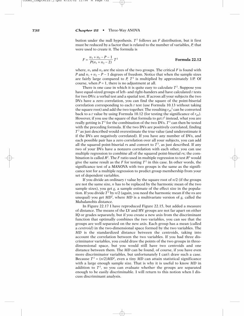
bution under the null hypothesis. T 2 follows an F distribution, but it firstmust be reduced by a factor that is related to the number of variables, P, thatwere used to create it. The formula is

F = T 2 Formula 22.12

where, n1 and n2 are the sizes of the two groups. The critical F is found withP and n1 + n2 − P − 1 degrees of freedom. Notice that when the sample sizesare fairly large compared to P, T 2 is multiplied by approximately 1/P. Ofcourse, when P = 1, there is no adjustment at all.

There is one case in which it is quite easy to calculate T 2. Suppose youhave equal-sized groups of left- and right-handers and have calculated t testsfor two DVs: a verbal test and a spatial test. If across all your subjects the twoDVs have a zero correlation, you can find the square of the point-biserialcorrelation corresponding to each t test (use Formula 10.13 without takingthe square root) and add the two together. The resulting rpb

2 can be convertedback to a t value by using Formula 10.12 (for testing the significance of rpb).However, if you use the square of that formula to get t2 instead, what you arereally getting is T 2 for the combination of the two DVs. T 2 can then be testedwith the preceding formula. If the two DVs are positively correlated, findingT 2 as just described would overestimate the true value (and underestimate itif the DVs are negatively correlated). If you have any number of DVs, andeach possible pair has a zero correlation over all your subjects, you can addall the squared point-biserial rs and convert to T 2, as just described. If anytwo of your DVs have a nonzero correlation with each other, you can usemultiple regression to combine all of the squared point-biserial rs; the com-bination is called R2. The F ratio used in multiple regression to test R2 wouldgive the same result as the F for testing T 2 in this case. In other words, thesignificance test of a MANOVA with two groups is the same as the signifi-cance test for a multiple regression to predict group membership from yourset of dependent variables.

If you divide an ordinary t value by the square root of n/2 (if the groupsare not the same size, n has to be replaced by the harmonic mean of the twosample sizes), you get g, a sample estimate of the effect size in the popula-tion. If you divide T 2 by n/2 (again, you need the harmonic mean if the ns areunequal) you get MD2, where MD is a multivariate version of g, called theMahalanobis distance.

In Figure 22.17 I have reproduced Figure 22.15, but added a measureof distance. The means of the LV and HV groups are not far apart on eitherIQ or grades separately, but if you create a new axis from the discriminantfunction that optimally combines the two variables, you can see that thegroups are well separated on the new axis. Each group has a mean (calleda centroid) in the two-dimensional space formed by the two variables. TheMD is the standardized distance between the centroids, taking intoaccount the correlation between the two variables. If you had three dis-criminator variables, you could draw the points of the two groups in three-dimensional space, but you would still have two centroids and onedistance between them. The MD can be found, of course, if you have evenmore discriminator variables, but unfortunately I can’t draw such a case.Because T 2 = (n/2)MD2, even a tiny MD can attain statistical significancewith a large enough sample size. That is why it is useful to know MD inaddition to T 2, so you can evaluate whether the groups are separatedenough to be easily discriminable. I will return to this notion when I dis-cuss discriminant analysis.

n1 + n2 − P − 1��P(n1 + n2 − 2)



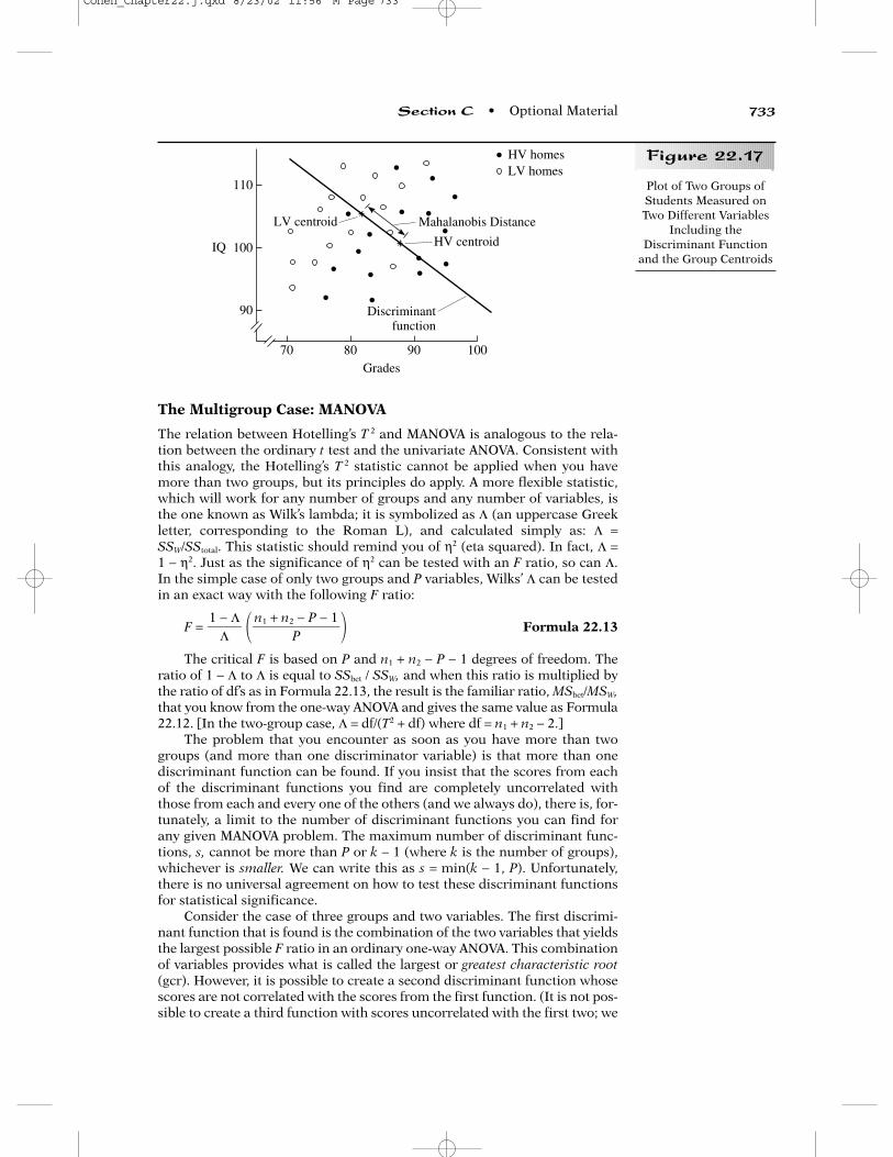
The Multigroup Case: MANOVA

The relation between Hotelling’s T 2 and MANOVA is analogous to the rela-tion between the ordinary t test and the univariate ANOVA. Consistent withthis analogy, the Hotelling’s T 2 statistic cannot be applied when you havemore than two groups, but its principles do apply. A more flexible statistic,which will work for any number of groups and any number of variables, isthe one known as Wilk’s lambda; it is symbolized as Λ (an uppercase Greekletter, corresponding to the Roman L), and calculated simply as: Λ =SSW/SStotal. This statistic should remind you of η2 (eta squared). In fact, Λ =1 − η2. Just as the significance of η2 can be tested with an F ratio, so can Λ.In the simple case of only two groups and P variables, Wilks’ Λ can be testedin an exact way with the following F ratio:

F = � � Formula 22.13

The critical F is based on P and n1 + n2 − P − 1 degrees of freedom. Theratio of 1 − Λ to Λ is equal to SSbet / SSW, and when this ratio is multiplied bythe ratio of df’s as in Formula 22.13, the result is the familiar ratio, MSbet/MSW,that you know from the one-way ANOVA and gives the same value as Formula22.12. [In the two-group case, Λ = df/(T2 + df) where df = n1 + n2 − 2.]

The problem that you encounter as soon as you have more than twogroups (and more than one discriminator variable) is that more than onediscriminant function can be found. If you insist that the scores from eachof the discriminant functions you find are completely uncorrelated withthose from each and every one of the others (and we always do), there is, for-tunately, a limit to the number of discriminant functions you can find forany given MANOVA problem. The maximum number of discriminant func-tions, s, cannot be more than P or k − 1 (where k is the number of groups),whichever is smaller. We can write this as s = min(k − 1, P). Unfortunately,there is no universal agreement on how to test these discriminant functionsfor statistical significance.

Consider the case of three groups and two variables. The first discrimi-nant function that is found is the combination of the two variables that yieldsthe largest possible F ratio in an ordinary one-way ANOVA. This combinationof variables provides what is called the largest or greatest characteristic root(gcr). However, it is possible to create a second discriminant function whosescores are not correlated with the scores from the first function. (It is not pos-sible to create a third function with scores uncorrelated with the first two; we

n1 + n2 − P − 1��

P1 − Λ�

Λ


Figure 22.17

110

100IQ

90

70 90 10080Grades

HV homesLV homes

Mahalanobis Distance

HV centroid

LV centroid

Discriminantfunction

Plot of Two Groups ofStudents Measured onTwo Different Variables

Including theDiscriminant Function

and the Group Centroids


know this because, for this case, s = 2). Each function corresponds to its ownlowercase lambda (λ), which can be tested for significance.

Having more than one little lambda to test is analogous to having sev-eral pairs of means to test in a one-way ANOVA—there is more than one wayto go about it while trying to keep Type I errors down and to maximizepower at the same time. The most common approach is to form an overallWilk’s Λ by pooling (through multiplication) the little lambdas and then totest Λ with an F ratio (the F ratio will follow an F distribution only approxi-mately if you have more than three groups and more than two DVs). Pillai’strace (sometimes called the Pillai-Bartlett statistic) is another way of poolingthe little lambdas, and it leads to a statistic that appears to be more robustthan Wilk’s Λ with respect to violations of the assumptions of MANOVA (seethe following). Therefore, statisticians tend to prefer Pillai’s trace especiallywhen sample sizes are small or unequal. A third way to pool the little lamb-das, Hotelling’s trace (sometimes called the Hotelling-Lawley trace), isreported and tested by the common statistical software packages but israrely used. All three of the statistics just described lead to similar F ratios inmost cases, and it is not very common to attain significance with one but notthe others. All of these statistics (including the one to be described next) canbe calculated when there are only two groups, but in that case they all leadto exactly the same F ratio.

A different approach to testing a multigroup MANOVA for significanceis to test only the gcr for significance, usually with Roy’s largest root test.Unfortunately, it is possible to attain significance with one of the “multiple-root” tests previously described, even though the gcr is not significant. Insuch a case, it is quite difficult to pinpoint the source of your multivariategroup differences, which is why some authors of statistical texts (notably,Harris, 1985) strongly prefer gcr tests. The gcr test is a reasonable alterna-tive when its assumptions are met and when the largest root (correspondingto the best discriminant function) is considerably larger than any of theothers. But consider the following situation. The three groups are normals,neurotics, and psychotics, and the two variables are degree of orientation toreality and inclination to seek psychotherapy. The best discriminant func-tion might consist primarily of the reality variable, with normals and neu-rotics being similar but very different from psychotics. The second functionmight be almost as discriminating as the first, but if it was weighted mostheavily on the psychotherapy variable, it would be discriminating the neu-rotics from the other two groups. When several discriminant functions areabout equally good, a multiple-root test, like Wilk’s lambda or Pillai’s trace,is likely to be more powerful than a gcr test.

The multiple-root test should be followed by a gcr test if you are inter-ested in understanding why your groups differ; as already mentioned, a sig-nificant multiple-root test does not guarantee a significant gcr test (Harris,1985). A significant gcr test, whether or not it is preceded by a multiple roottest, can be followed by a separate test of the next largest discriminant func-tion, and so on, until you reach a root that is not significant. (Alternatively,you can recalculate Wilk’s Λ without the largest root, test it for significance,and then drop the second largest and retest until Wilk’s Λ is no longer sig-nificant.) Each significant discriminant function (if standardized) can beunderstood in terms of the weight each of the variables has in that function(or the discriminant loading of each variable). I’ll say a bit more about thisin the section on discriminant analysis.

Any ANOVA design can be performed as a MANOVA; in fact, factorialMANOVAs are quite common. A different set of discriminant functions isfound for each main effect, as well as for the interactions. A significant two-



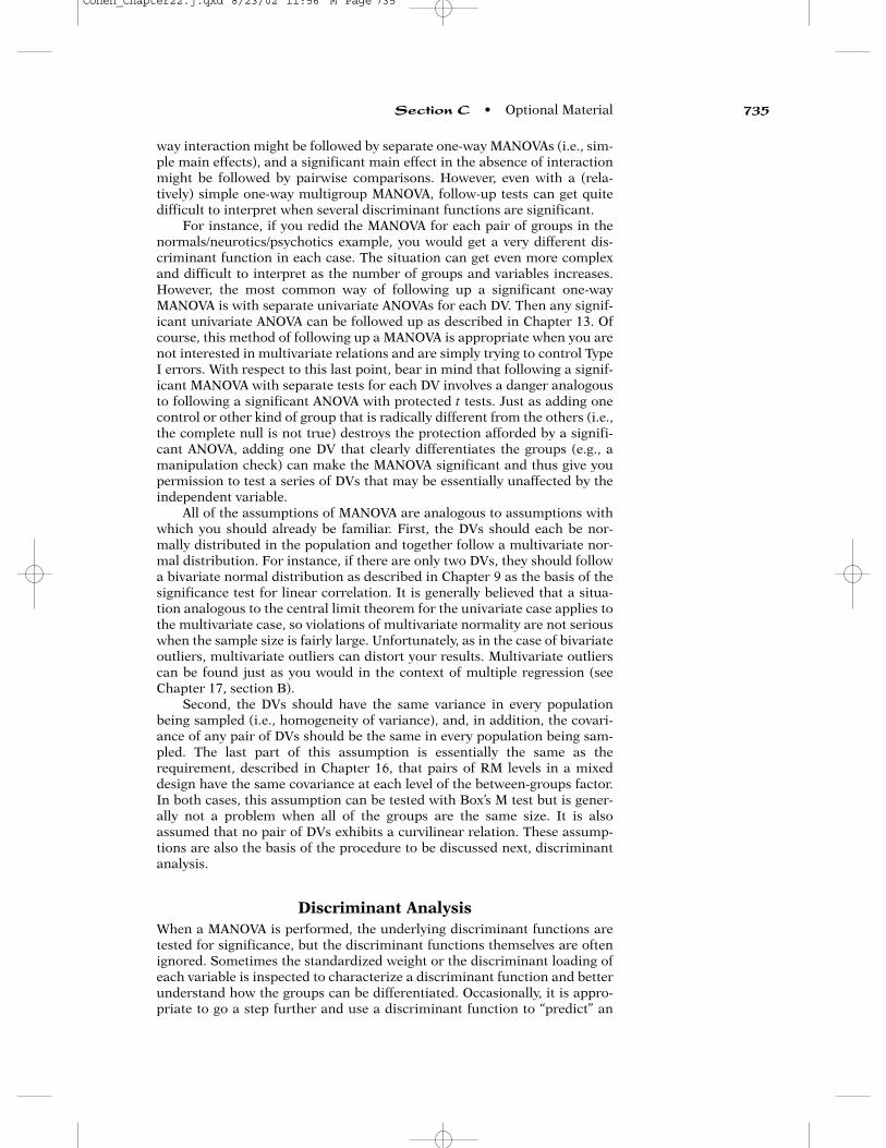
way interaction might be followed by separate one-way MANOVAs (i.e., sim-ple main effects), and a significant main effect in the absence of interactionmight be followed by pairwise comparisons. However, even with a (rela-tively) simple one-way multigroup MANOVA, follow-up tests can get quitedifficult to interpret when several discriminant functions are significant.

For instance, if you redid the MANOVA for each pair of groups in thenormals/neurotics/psychotics example, you would get a very different dis-criminant function in each case. The situation can get even more complexand difficult to interpret as the number of groups and variables increases.However, the most common way of following up a significant one-wayMANOVA is with separate univariate ANOVAs for each DV. Then any signif-icant univariate ANOVA can be followed up as described in Chapter 13. Ofcourse, this method of following up a MANOVA is appropriate when you arenot interested in multivariate relations and are simply trying to control TypeI errors. With respect to this last point, bear in mind that following a signif-icant MANOVA with separate tests for each DV involves a danger analogousto following a significant ANOVA with protected t tests. Just as adding onecontrol or other kind of group that is radically different from the others (i.e.,the complete null is not true) destroys the protection afforded by a signifi-cant ANOVA, adding one DV that clearly differentiates the groups (e.g., amanipulation check) can make the MANOVA significant and thus give youpermission to test a series of DVs that may be essentially unaffected by theindependent variable.

All of the assumptions of MANOVA are analogous to assumptions withwhich you should already be familiar. First, the DVs should each be nor-mally distributed in the population and together follow a multivariate nor-mal distribution. For instance, if there are only two DVs, they should followa bivariate normal distribution as described in Chapter 9 as the basis of thesignificance test for linear correlation. It is generally believed that a situa-tion analogous to the central limit theorem for the univariate case applies tothe multivariate case, so violations of multivariate normality are not seriouswhen the sample size is fairly large. Unfortunately, as in the case of bivariateoutliers, multivariate outliers can distort your results. Multivariate outlierscan be found just as you would in the context of multiple regression (seeChapter 17, section B).

Second, the DVs should have the same variance in every populationbeing sampled (i.e., homogeneity of variance), and, in addition, the covari-ance of any pair of DVs should be the same in every population being sam-pled. The last part of this assumption is essentially the same as therequirement, described in Chapter 16, that pairs of RM levels in a mixeddesign have the same covariance at each level of the between-groups factor.In both cases, this assumption can be tested with Box’s M test but is gener-ally not a problem when all of the groups are the same size. It is alsoassumed that no pair of DVs exhibits a curvilinear relation. These assump-tions are also the basis of the procedure to be discussed next, discriminantanalysis.

Discriminant AnalysisWhen a MANOVA is performed, the underlying discriminant functions aretested for significance, but the discriminant functions themselves are oftenignored. Sometimes the standardized weight or the discriminant loading ofeach variable is inspected to characterize a discriminant function and betterunderstand how the groups can be differentiated. Occasionally, it is appro-priate to go a step further and use a discriminant function to “predict” an



individual’s group membership; that procedure is called discriminant analy-sis. Discriminant analysis (DA) is to MANOVA as linear regression and pre-diction is to merely testing the significance of the linear relation betweentwo variables. As in the case of MANOVA, DA is much simpler in the two-group case, so that is where I’ll begin.

In a typical two-group MANOVA situation you might be comparingright- and left-handers on a battery of cognitive tasks, especially those tasksknown to be lateralized in the brain, to see if the two groups are significantlydifferent. You want to see if handedness has an impact on cognitive func-tioning. The emphasis of discriminant analysis is different. In discriminantanalysis you want to find a set of variables that differentiates the two groupsas well as possible. You might start with a set of variables that seem likely todiffer between the two groups and perform a stepwise discriminant analysisin which variables that contribute well to the discrimination (based on sta-tistical tests) are retained and those which contribute little are dropped (thisprocedure is similar to stepwise regression, which is described in much detailin Chapter 17). The weights of the resulting standardized (i.e., variables areconverted to z scores) discriminant function (also called a canonical variatebecause discriminant analysis is a special case of canonical correlation), ifsignificant, can be compared to get an idea of which variables are doing thebest job of differentiating the two groups. (The absolute sizes of the weights,but not their relation to one other, are arbitrary and are usually “normalized”so that the squared weights sum to 1.0). Unfortunately, highly correlated DVscan lead to unreliable and misleading relative weights, so an effort is gener-ally made to combine similar variables or delete redundant ones.

Depending on your purpose for performing a discriminant analysis, youmay want to add a final step: classification. This is fairly straightforward inthe two-group case. If you look again at Figure 22.17, you can see that theresult of a discriminant analysis with two groups is to create a new dimen-sion upon which each subject has a score. It is this dimension that tends tomaximize the separation of the two groups while minimizing variabilitywithin groups (eta squared is maximized, which is the same in this case asR2, where R is both the canonical correlation and the coefficient of multiplecorrelation). This dimension can be used for classification by selecting a cut-off score; every subject below the cutoff score is classified as being in onegroup, whereas everyone above the cutoff is classified as being in the othergroup. The simplest way to choose a cutoff score is to halve the distancebetween the two group centroids. In Figure 22.17 this cutoff score results intwo subjects being misclassified. The most common way to evaluate thesuccess of a classification scheme is to calculate the rate of misclassification.

If the populations represented by your two groups are unequal in size, orthere is a greater cost for one type of classification error than the other (e.g.,judging erroneously from a battery of tests that a child be placed in special edu-cation may have a different “cost” from erroneously denying special educationto a child who needs it), the optimal cutoff score may not be in the middle.There are also alternative ways to make classifications, such as measuring theMahalanobis distance between each subject and each of the two centroids. But,you may be wondering, why all this effort to classify subjects when you alreadyknow what group they are in? The first reason is that the rate of correct classi-fication is one way of evaluating the success of your discriminant analysis.

The second reason is analogous to linear regression. The regressionequation is calculated for subjects for whom you know both X and Y scores,but it can be used to predict the Y scores for new subjects for whom you onlyhave X scores. Similarly, the discriminant function and cutoff score for yourpresent data can be used to classify future subjects whose correct group is



not known. For instance, you measure a sample of babies on a battery ofperceptual tests, wait a few years until it is known which children havelearning difficulties, and perform a discriminant analysis. Then new babiesare tested and classified according to the results of the original study. If yourmisclassification rate is low, you can confidently recommend remedialmeasures for babies classified in the (future) learning disabled group andperhaps eliminate the disability before the child begins school. Of course,classification can also be used retroactively, for instance to classify earlyhominids as Neanderthal or Cro Magnon based on various skeletal measures(assuming there are some specimens you can be relatively sure about).

With two significant discriminant functions and three groups, the cen-troids of the groups will not fall on one straight line, but they can be locatedon a plane formed by the two (orthogonal) discriminant functions. Figure22.18 depicts the normals/neurotics/psychotics example; each discriminantfunction is named after the DV that carries the largest weight on it. Insteadof a cutoff score, classification is made by assigning a region around eachgroup, such that the regions are mutually exclusive and exhaustive (i.e.,every subject must land in one, but only one, region). The regions displayedin Figure 22.18 form what is called a territorial map. Of course, it becomesimpossible to draw the map in two dimensions as you increase the numberof groups and the number of variables, but it is possible to extend the gen-eral principle of classification to any number of dimensions. Unfortunately,having several discriminant functions complicates the procedure for testingtheir significance, as discussed under the topic of MANOVA.

Using MANOVA to Test Repeated MeasuresThere is one more application of MANOVA that is becoming too popular tobe ignored: MANOVA can be used as a replacement for the univariate one-way RM ANOVA. To understand how this is done, it will help to recall thedirect-difference method for the matched t test. By creating difference scores,a two-sample test is converted to a one-sample test against the null hypothe-sis that the mean of the difference scores is zero in the population. Now sup-


Figure 22.18Inclination to Seek Psychotherapy

High

Low

Centroid for Neurotics

Orientation to Reality

Centroid for Psychotics

Centroid for Normals

Low High

A Territorial Map ofThree Groups of Subjects

Measured Along TwoDiscriminant Functions


pose that your RM factor has three levels (e.g., before, during, and after sometreatment). You can create two sets of difference scores, such as before-during (BD), and during-after (DA). (The third difference score, before-after,would be exactly the same as the sum of the other two—because there areonly two df, there can only be two sets of nonredundant difference scores.)Even though you now have two dependent variables, you can still perform aone-sample test to determine whether your difference scores differ signifi-cantly from zero. This can be accomplished by performing a one-sampleMANOVA. The MANOVA procedure will “find” the weighted combination ofBD and DA that produces a mean score as far from zero as possible.

Finding the best weighted average of the difference scores sounds likean advantage over the ordinary RM ANOVA, which just deals with ordinaryaverages, and it can be—but you pay a price for the “customized” combina-tions of MANOVA. The price is a considerable loss of degrees of freedom inthe error term. For a one-way RM ANOVA, dferror equals (n − 1)(P − 1), wheren is the number of different subjects (or matched blocks), and P is the num-ber of levels of the RM factor. If you perform the analysis as a one-sampleMANOVA on P − 1 difference scores, dferror drops to n − P + 1 (try a few val-ues for n and P, and you will notice the differences). In fact, you cannot usethe MANOVA approach to RM analysis when the number of subjects is lessthan the number of RM levels (i.e., n < P); your error term won’t have anydegrees of freedom. And when n is only slightly greater than P, the power ofthe MANOVA approach is usually less than the RM ANOVA.

So, why is the MANOVA alternative strongly encouraged by many stat-isticians and becoming increasingly popular? Because MANOVA does nottake a simple average of the variances of the possible difference scores andtherefore does not assume that these variances are all the same (the spheric-ity assumption), the MANOVA approach is not vulnerable to the Type I errorinflation that occurs with RM ANOVA when sphericity does not exist in thepopulation. Of course, there are adjustments you can make to RM ANOVA,as you learned in Chapter 15, but now that MANOVA is so easy to use on RMdesigns (thanks to recent advances in statistical software), it is a reasonablealternative whenever your sample is fairly large. As I mentioned in Chapter15, it is not an easy matter to determine which approach has greater powerfor fairly large samples and fairly large departures from sphericity. Conse-quently, it has been suggested that in such situations both procedures beroutinely performed and the better of the two accepted in each case. This isa reasonable approach with respect to controlling Type I errors only if youuse half of your alpha for each test (usually .025 for each), and you evaluatethe RM ANOVA with the ε adjustment of the df.

Complex MANOVA

The MANOVA approach can be used with designs more complicated than theone-way RM ANOVA. For instance, in a two-way mixed design, MANOVA canbe used to test the main effect of the RM factor, just as described for the one-way RM ANOVA. In addition, the interaction of the mixed design can be testedby forming the appropriate difference scores separately for each group of sub-jects and then using a two- or multigroup (i.e., one-way) MANOVA. A signifi-cant one-way MANOVA indicates that the groups differ in their level-to-levelRM differences, which demonstrates a group by RM interaction. The MANOVAapproach can also be extended to factorial RM ANOVAs (as described at theend of Section A in this chapter) and designs that are called doubly multivari-ate. The latter design is one in which a set of DVs is measured at several pointsin time or under several different conditions within the same subjects.



1. In the simplest form of multivariate analysis of variance (MANOVA)there are two independent groups of subjects measured on two depend-ent variables. The MANOVA procedure finds the weighted combinationof the two DVs that yields the largest possible t value for comparing thetwo groups. The weighted combination of (two or more) DVs is calledthe discriminant function, and the t value that is based on it, whensquared, is called Hotelling’s T2.

2. T2 can be converted into an F ratio for significance testing; the larger thenumber of DVs that contributed to T2, the more the F ratio is reducedbefore testing. The T2 value is a product of (half) the sample size, and aneffect size measure like g (called the Mahalanobis distance), whichmeasures the multivariate separation between the two groups.

3. When there are more than two independent groups, the T2 statistic is usu-ally replaced by Wilks’ Λ, the ratio of error variability (i.e., SSW) to totalvariability (you generally want Λ to be small). However, when there aremore than two groups and more than one DV, there is more than one dis-criminant function that can be found (the maximum number is one lessthan the number of groups or the number of DVs, whichever is smaller)and therefore more than one lambda to calculate. The most common wayto test a MANOVA for significance is to pool the lambdas from all the pos-sible discriminant functions and test the pooled Wilks’ Λ with an approx-imate F ratio (Pillai’s trace is a way of combining the lambdas that is morerobust when the assumptions of MANOVA are violated).

4. When there are more than one discriminant function that can be found,the first one calculated is the one that produces the largest F ratio; thisone is called the greatest characteristic root (gcr). An alternative to testingthe pooled lambdas is to test only the gcr (usually with Roy’s test). Thegcr test has an advantage when one of the discriminant functions ismuch larger than all of the others. If, in addition to finding out whetherthe groups differ significantly, you want to explore and interpret the dis-criminant functions, you can follow a significant gcr test by testing suc-cessively smaller discriminant functions until you come to one that is notsignificant. Alternatively, you can follow a significant test of the pooledlambdas by dropping the largest discriminant function, retesting, andcontinuing the process until the pooled lambda is no longer significant.

5. The most common use of MANOVA is to control Type I errors when test-ing several DVs in the same experiment; a significant MANOVA is thenfollowed by univariate tests of each DV. However, if the DVs are virtuallyuncorrelated, or one of the DVs very obviously differs among thegroups, it may be more legitimate (and powerful) to skip the MANOVAtest and test all of the DVs separately, using the Bonferroni adjustment.Another use for MANOVA is to find combinations of DVs that discrimi-nate the groups more efficiently than any one DV. In this case you wantto avoid using DVs that are highly correlated because this will lead tounreliable discriminant functions.

6. If you want to use a set of DVs to predict which of several groups a par-ticular subject is likely to belong to, you want to use a procedure calleddiscriminant analysis (DA). DA finds discriminant functions, as inMANOVA, and then uses these functions to create territorial maps,regions based on combinations of the DVs that tend to maximally cap-ture the groups. With only two groups, a cutoff score on a single dis-criminant function can be used to classify subjects as likely to belong toone group or the other (e.g., high school dropouts or graduates). To theextent that the groups tend to differ on the discriminant function, therate of misclassification will be low, and the DA will be considered suc-


CSUMMARY


cessful. DA can also be used as a theoretical tool to understand howgroups differ in complex ways involving several DVs simultaneously.

7. It may not be efficient or helpful to use all of the DVs you have availablefor a particular discriminant analysis. There are procedures, such asstepwise discriminant analysis, that help you systematically to find thesubset of your DVs that does the best job of discriminating among yourgroups. These stepwise procedures are similar to the procedures forstepwise multiple regression.

8. The MANOVA procedure can be used as a substitute for the one-way RMANOVA by forming difference scores (between pairs of RM levels) andthen finding the weighted combination of these difference scores thatbest discriminates them from zero (the usual expectation under the nullhypothesis). Because MANOVA does not require the sphericity assump-tion, the df does not have to be conservatively adjusted. However, in theprocess of “customizing” the combination of difference scores,MANOVA has fewer degrees of freedom available than the correspon-ding RM ANOVA [n − P + 1 for MANOVA, but (n − 1)(P − 1) for RMANOVA]. MANOVA cannot be used in place of RM ANOVA when thereare fewer subjects than treatment levels, and MANOVA is not recom-mended when the number of subjects is only slightly larger than thenumber of treatments. However, when the sample size is relatively large,MANOVA is likely to have more power than RM ANOVA, especially if thesphericity assumption does not seem to apply to your data.


EXERCISES

1. In a two-group experiment, three dependentvariables were combined to give a maximumt value of 3.8.a. What is the value of T 2?b. Assuming both groups contain 12 subjects

each, test T 2 for significance.c. Find the Mahalanobis distance between

these two groups.d. Recalculate parts b and c if the sizes of the

two groups are 10 and 20.2. In a two-group experiment, four dependent

variables were combined to maximize theseparation of the groups. SSbet = 55 and SSW =200.a. What is the value of Λ?b. Assuming one group contains 20 subjects

and the other 25 subjects, test Λ for signif-icance.

c. What is the value of T 2?d. Find the Mahalanobis distance between

these two groups.3. Nine men and nine women are tested on two

different variables. In each case, the t testfalls short of significance; t = 1.9 for the firstDV, and 1.8 for the second. The correlationbetween the two DVs over all subjects is zero.a. What is the value of T 2?

b. Find the Mahalanobis distance betweenthese two groups.

c. What is the value of Wilks’ Λ?d. Test T 2 for significance. Explain the

advantage of using two variables ratherthan one to discriminate the two groupsof subjects.

4. What is the maximum number of (orthogo-nal) discriminant functions that can befound whena. There are four groups and six dependent

variables?b. There are three groups and eight depend-

ent variables?c. There are seven groups and five depend-

ent variables?5. Suppose you have planned an experiment in

which each of your 12 subjects is measuredunder six different conditions.a. What is the df for the error term if you

perform a one-way RM ANOVA on yourdata?

b. What is the df for the error term if youperform a MANOVA on your data?

6. Suppose you have planned an experiment inwhich each of your 20 subjects is measuredunder four different conditions.


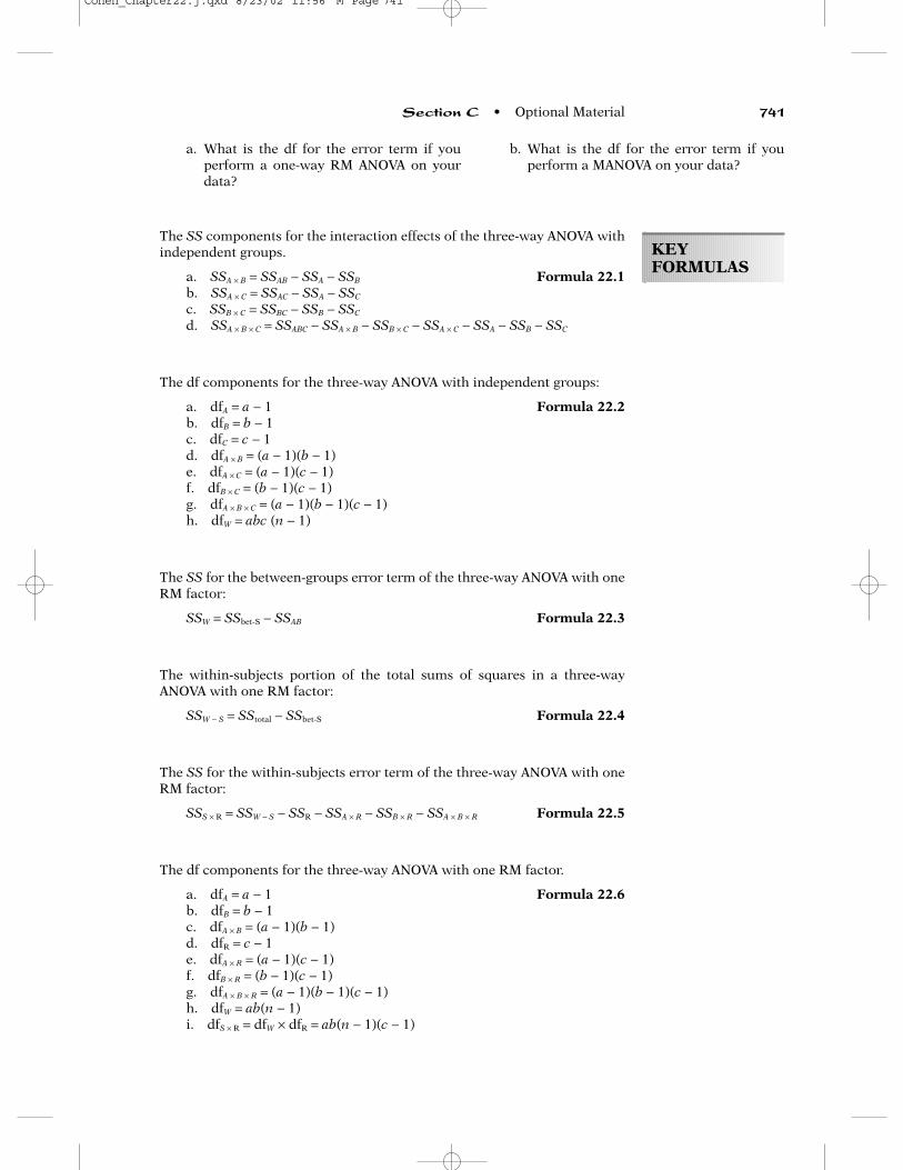
a. What is the df for the error term if youperform a one-way RM ANOVA on yourdata?

b. What is the df for the error term if youperform a MANOVA on your data?


KEYFORMULAS

The SS components for the interaction effects of the three-way ANOVA withindependent groups.

a. SSA × B = SSAB − SSA − SSB Formula 22.1b. SSA × C = SSAC − SSA − SSC

c. SSB × C = SSBC − SSB − SSC

d. SSA × B × C = SSABC − SSA × B − SSB × C − SSA × C − SSA − SSB − SSC

The df components for the three-way ANOVA with independent groups:

a. dfA = a − 1 Formula 22.2b. dfB = b − 1c. dfC = c − 1d. dfA × B = (a − 1)(b − 1)e. dfA × C = (a − 1)(c − 1)f. dfB × C = (b − 1)(c − 1)g. dfA × B × C = (a − 1)(b − 1)(c − 1)h. dfW = abc (n − 1)

The SS for the between-groups error term of the three-way ANOVA with oneRM factor:

SSW = SSbet-S − SSAB Formula 22.3

The within-subjects portion of the total sums of squares in a three-wayANOVA with one RM factor:

SSW − S = SStotal − SSbet-S Formula 22.4

The SS for the within-subjects error term of the three-way ANOVA with oneRM factor:

SSS × R = SSW − S − SSR − SSA × R − SSB × R − SSA × B × R Formula 22.5

The df components for the three-way ANOVA with one RM factor.

a. dfA = a − 1 Formula 22.6b. dfB = b − 1c. dfA × B = (a − 1)(b − 1)d. dfR = c − 1e. dfA × R = (a − 1)(c − 1)f. dfB × R = (b − 1)(c − 1)g. dfA × B × R = (a − 1)(b − 1)(c − 1)h. dfW = ab(n − 1)i. dfS × R = dfW × dfR = ab(n − 1)(c − 1)


The F ratios for the three-way ANOVA with one RM factor:


b. FB =

c. FA × B =

d. FR =

e. FA × R =

f. FB × R =

g. FA × B × R =

The SS for the between-groups error term of the three-way ANOVA with twoRM factors:

SSW = SSS − SSA Formula 22.8

The SS components for the within-subjects error terms of the three-wayANOVA with two RM factors:

a. SSQ × S = SSQS − SSQ − SSS − SSA × Q Formula 22.9

b. SSR × S = SSRS − SSR − SSS − SSA × R

c. SSQ × R × S = SStotal − SSAQR − SSW − SSQ × S − SSR × S

The df components for the three-way ANOVA with two RM factors:

a. dfA = a − 1 Formula 22.10b. dfQ = q − 1c. dfR = r − 1d. dfA × Q = (a − 1)(q − 1)e. dfA × R = (a − 1)(r − 1)f. dfQ × R = (q − 1)(r − 1)g. dfA × Q × R = (a − 1)(q − 1)(r − 1)h. dfW = a(n − 1)i. dfQ × S = dfQ × dfW = a(q − 1)(n − 1)j. dfR × S = dfR × dfW = a(r − 1)(n − 1)k. dfQ × R × S = dfQ × dfR × dfW = a(q − 1)(r − 1)(n − 1)

MSA × B × R��

MSS × R

MSB × R�MSS × R

MSA × R�MSS × R

MSR�MSS × R

MSA × B�

MSW

MSB�MSW

MSA�MSW



The F ratios for the three-way ANOVA with two RM factors:


b. FQ =

c. FR =

d. FA × Q =

e. FA × R =

f. FQ × R =

g. FA × Q × R =

The F ratio for testing the significance of T2 calculated for P dependent vari-ables and two independent groups:

F = T2 Formula 22.12

The F ratio for testing the significance of Wilks’ lambda calculated for Pdependent variables and two independent groups:

F = � � Formula 22.13n1 + n2 − P − 1��

P1 − Λ�

Λ

n1 + n2 − P − 1��P(n1 + n2 − 2)

MSA × Q × R��MSQ × R × S

MSQ × R��MSQ × R × S

MSA × R�MSR × S

MSA × Q�MSQ × S

MSR�MSR × S

MSQ�MSQ × S

MSA�MSW

Key Formulas • Optional Material 743


REFERENCESBanaji, M. R., & Hardin, C. D. (1996). Automatic stereotyping. Psychological

Science, 7, 136–141.Bruder, G. E., Stewart, J. W., Mercier, M. A., Agosti, V., Leite, P., Donovan, S.,

& Quitkin, F. M. (1997). Outcome of cognitive-behavioral therapy fordepression: Relation to hemispheric dominance for verbal processing.Journal of Abnormal Psychology, 106, 138–144.

Cole, D. A., Maxwell, S. E., Arvey, R., & Salas, E. (1994). How the power ofMANOVA can both increase and decrease as a function of the intercor-relations among the dependent variables. Psychological Bulletin, 115,465–474.

Harris, R. J. (1985). A primer of multivariate statistics (2nd ed.). Orlando,Florida: Academic Press.

Hays, W. L. (1994). Statistics (5th ed.). New York: Harcourt Brace CollegePublishing.

Huynh, H., & Mandeville, G. K. (1979). Validity conditions in repeated meas-ures designs. Psychological Bulletin, 86, 964–973.

Marlowe, C. M., Schneider, S. L., & Nelson, C. E. (1996). Gender and attrac-tiveness biases in hiring decisions: Are more experienced managers lessbiased? Journal of Applied Psychology, 81, 11–21.



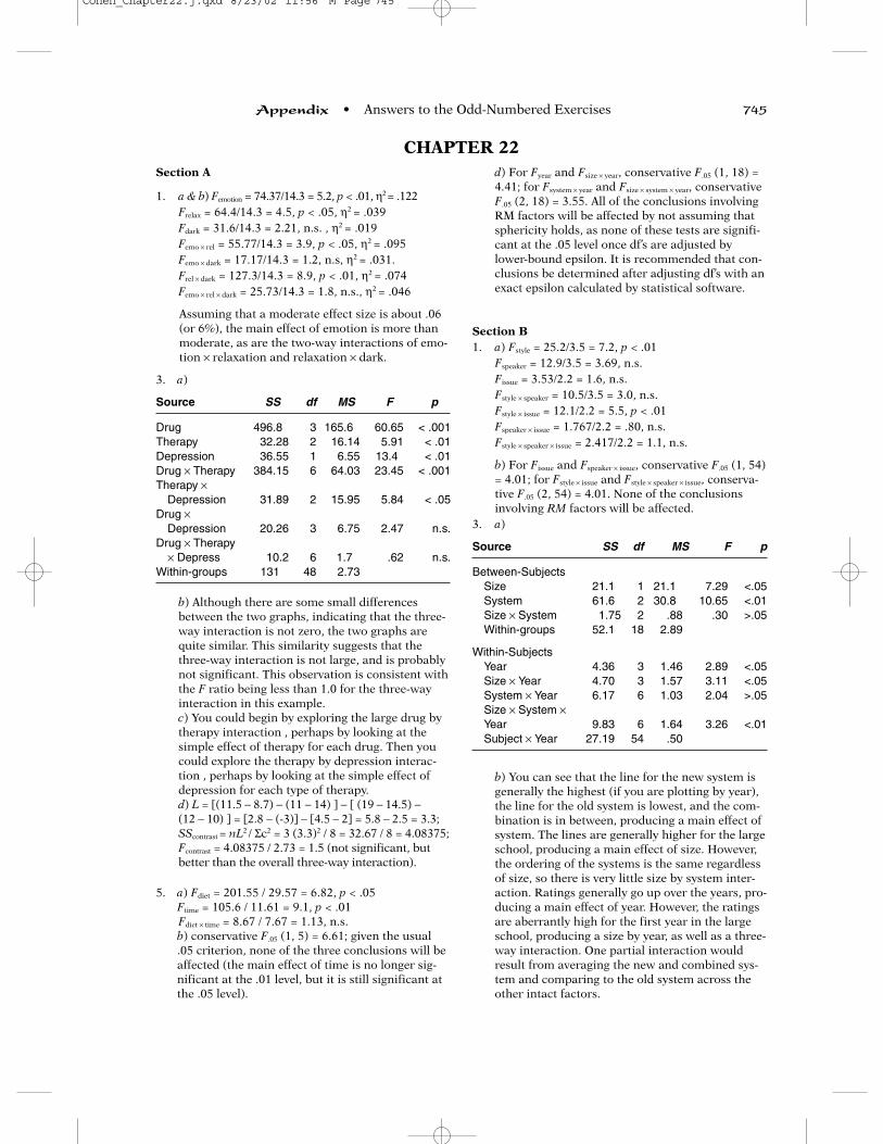
Section A

1. a & b) Femotion = 74.37/14.3 = 5.2, p < .01, η2 = .122Frelax = 64.4/14.3 = 4.5, p < .05, η2 = .039Fdark = 31.6/14.3 = 2.21, n.s. , η2 = .019Femo × rel = 55.77/14.3 = 3.9, p < .05, η2 = .095Femo × dark = 17.17/14.3 = 1.2, n.s, η2 = .031.Frel × dark = 127.3/14.3 = 8.9, p < .01, η2 = .074Femo × rel × dark = 25.73/14.3 = 1.8, n.s., η2 = .046

Assuming that a moderate effect size is about .06(or 6%), the main effect of emotion is more thanmoderate, as are the two-way interactions of emo-tion × relaxation and relaxation × dark.

3. a)

Source SS df MS F p

Drug 496.8 3 165.6 60.65 < .001Therapy 32.28 2 16.14 5.91 < .01Depression 36.55 1 6.55 13.4 < .01Drug × Therapy 384.15 6 64.03 23.45 < .001Therapy ×

Depression 31.89 2 15.95 5.84 < .05Drug ×

Depression 20.26 3 6.75 2.47 n.s.Drug × Therapy

× Depress 10.2 6 1.7 .62 n.s.Within-groups 131 48 2.73

b) Although there are some small differencesbetween the two graphs, indicating that the three-way interaction is not zero, the two graphs arequite similar. This similarity suggests that thethree-way interaction is not large, and is probablynot significant. This observation is consistent withthe F ratio being less than 1.0 for the three-wayinteraction in this example. c) You could begin by exploring the large drug bytherapy interaction , perhaps by looking at thesimple effect of therapy for each drug. Then youcould explore the therapy by depression interac-tion , perhaps by looking at the simple effect ofdepression for each type of therapy.d) L = [(11.5 − 8.7) − (11 − 14) ] − [ (19 − 14.5) −(12 − 10) ] = [2.8 − (-3)] − [4.5 − 2] = 5.8 − 2.5 = 3.3;SScontrast = nL2 / Σc2 = 3 (3.3)2 / 8 = 32.67 / 8 = 4.08375;Fcontrast = 4.08375 / 2.73 = 1.5 (not significant, butbetter than the overall three-way interaction).

5. a) Fdiet = 201.55 / 29.57 = 6.82, p < .05Ftime = 105.6 / 11.61 = 9.1, p < .01Fdiet × time = 8.67 / 7.67 = 1.13, n.s.b) conservative F.05 (1, 5) = 6.61; given the usual.05 criterion, none of the three conclusions will beaffected (the main effect of time is no longer sig-nificant at the .01 level, but it is still significant atthe .05 level).

d) For Fyear and Fsize × year, conservative F.05 (1, 18) =4.41; for Fsystem × year and Fsize × system × year, conservativeF.05 (2, 18) = 3.55. All of the conclusions involvingRM factors will be affected by not assuming thatsphericity holds, as none of these tests are signifi-cant at the .05 level once df’s are adjusted bylower-bound epsilon. It is recommended that con-clusions be determined after adjusting df’s with anexact epsilon calculated by statistical software.

Section B1. a) Fstyle = 25.2/3.5 = 7.2, p < .01

Fspeaker = 12.9/3.5 = 3.69, n.s.Fissue = 3.53/2.2 = 1.6, n.s. Fstyle × speaker = 10.5/3.5 = 3.0, n.s.Fstyle × issue = 12.1/2.2 = 5.5, p < .01Fspeaker × issue = 1.767/2.2 = .80, n.s.Fstyle × speaker × issue = 2.417/2.2 = 1.1, n.s.

b) For Fissue and Fspeaker × issue, conservative F.05 (1, 54)= 4.01; for Fstyle × issue and Fstyle × speaker × issue, conserva-tive F.05 (2, 54) = 4.01. None of the conclusionsinvolving RM factors will be affected.

3. a)

Source SS df MS F p

Between-SubjectsSize 21.1 1 21.1 7.29 <.05System 61.6 2 30.8 10.65 <.01Size × System 1.75 2 .88 .30 >.05Within-groups 52.1 18 2.89

Within-SubjectsYear 4.36 3 1.46 2.89 <.05Size × Year 4.70 3 1.57 3.11 <.05System × Year 6.17 6 1.03 2.04 >.05Size × System × Year 9.83 6 1.64 3.26 <.01Subject × Year 27.19 54 .50

b) You can see that the line for the new system isgenerally the highest (if you are plotting by year),the line for the old system is lowest, and the com-bination is in between, producing a main effect ofsystem. The lines are generally higher for the largeschool, producing a main effect of size. However,the ordering of the systems is the same regardlessof size, so there is very little size by system inter-action. Ratings generally go up over the years, pro-ducing a main effect of year. However, the ratingsare aberrantly high for the first year in the largeschool, producing a size by year, as well as a three-way interaction. One partial interaction wouldresult from averaging the new and combined sys-tem and comparing to the old system across theother intact factors.

Appendix • Answers to the Odd-Numbered Exercises 745

CHAPTER 22


c) Given the significant three-way interaction, itwould be reasonable to look at simple interactioneffects—perhaps, the system by year interactionfor each school size. This two-way interactionwould likely be significant only for the largeschool, and would then be followed by testing thesimple main effects of year for each system. To becautious about sphericity, you can use an errorterm based only on the conditions included in thatfollow-up test. There are other legitimate possibili-ties for exploring simple effects, as well.

5. a)

Source SS df MS F p

Between-groupsBackground .93 1 .93 .22 n.s.Within-group 42.85 10 4.29

Within-subjectsAffect 13.72 2 6.86 7.04 <.01Background ×

Affect 19.02 2 9.51 9.76 <.01Subject ×

Affect 19.48 20 .97

Image 131.06 2 65.53 51.21 <.001Background ×

Image .24 2 .12 .09 n.s.Subject ×

Image 25.59 20 1.28

Affect × Image 18.39 4 4.60 4.71 <.01Back × Affect

× Image 2.32 4 .58 .59 n.s.Subject × Affect

× Image 39.07 40 .98

b) The conservative F.05 (1, 10) = 4.96 for all of theF’s involving an RM factor (i.e., all F’s except themain effect of background music). The F for theaffect by image interaction is no longer significantwith a conservative adjustment to df; a more exactadjustment of df is recommended in this case.None of the other conclusions are affected (exceptthat the main effect of affect and its interactionwith background music are significant at the .05,instead of .01 level after the conservative adjust-ment).c) If you plot affect on the X axis, you can see alarge main effect of image, because the three

image lines are clearly and consistently separate.You can see some affect by image interaction inthat the lines are not parallel, especially due tothe medium line. There is a noticeable back-ground by affect interaction, because for thehappy music condition, recall of happy words ishigher, whereas sad word recall is higher duringthe sad background music. The main effect ofaffect is not obvious with affect plotted on thehorizontal axis. The medium/low (or high/low) bysad/neutral by background contrast appears to beone of the largest of the possible 2 × 2 × 2 interac-tion contrasts.d) The three-way interaction is not significant, sothe focus shifts to the two significant two-wayinteractions: affect by image and affect by back-ground. Averaging across the imageability levels,one could look at the simple effects of affect foreach type of background music; averaging acrossthe background levels, one could look at the simpleeffects of affect for each level of imageability. Sig-nificant simple effects can then be followed byappropriate pairwise comparisons. There are otherlegitimate possibilities, as well.

Section C

1. a) T 2 = 3.82 = 14.44b) F = 14.44 * (24 − 3 − 1) / 3 (22) = 4.376 > F.05

(3, 20) = 3.1, so T 2 is significant at the .05 level.c) MD2 = T 2 /n/2 = 14.44/6 = 2.407; MD = 1.55d) F = 14.44 * (30 − 3 − 1)/3 (28) = 4.47; harmonicmean of 10 and 20 = 13.33, MD2 = 14.44/13.33/2 =2.167; MD = 1.47

3. a) R2 (the sum of the two rpb2’s) = .184 + .168 = .352;

T 2 = 16 * [.352/(1 − .352)] = 8.69b) MD2 = 8.69/4.5 = 1.93; MD = 1.39c) Λ = 16/(8.69 + 16) = .648d) F = (15/32) * 8.69 = 4.07 > F.05 (2, 15) = 3.68, soT 2 is significant at the .05 level. As in multipleregression with uncorrelated predictors, each DVcaptures a different part of the variance betweenthe two groups; together the two DV’s account formuch more variance than either one alone.

5. a) df = (6 − 1) (12 − 1) = 5 * 11 = 55b) df = 12 − 6 + 1 = 7



Documents

Three-way ANOVA Chapter