Embed Size (px)
Citation preview

AD-R171 259 THREE-DIMENSIONAL ANALYTICAL MODELING OF /DIFFUSION-LIMITED SOLUTE TRANSPORT(U) AIR FORCE INST OFTECH NRIGHT-PATTERSON AFB OH M N GOLTZ JUL 96
UNCL ASS FI EAFI T/C96 i /NR 96-3 F/O /0 NL

MICROCOPY Nismuo~Uft Is I NMIGATNOWSk gAU '. J#AKAA *
* .me

SECURITY CLASSIFICATION OF THIS PAGE (*7jen Date.Entered), 0. 0
READ INSTRUCTIO..REPORT DOCUMENTATION PAGE BEFORE COMfPLETING FORMIREPORT NUMBER 2. GOVT ACCESSION No. 3. RECIPIENT'S CATALOG NUMBER
4. TITLE (and Subtitle) S. TYPE OF REPORT & PERIOD COVEREDThree-Dimensional Analytical Modeling of T7~DSETTO
Diffusion-Limited Solute Transport _______________
Ln S. PERFORMING ORG. REPORT N UMBER
7. AUTHOR(s) U. CONTRACT OR GRANT NUMBER(&)
P% Mark Neil Goltz
9. PERFORMING ORGANIZATION NAME AND ADDRESS 10. PROGRAM ELEMENT. PROJECT, TASKAREA & WORK UNIT NUMBERS
AFIT STUDENT AT: Stanford University
S It. CONTROLLING OFFICE NAME AND ADDRESS 12. REPORT DATE
AFIT /NR 1986
WPAFB OH 45433-6583 13. NUMBER OF PAGES
____ ___ ___ ___ ____ ___ ___ ___ ____ ___ ___ ___ 172
14. MONITORING AGENCY NAME A ADORESS(it different from Controlling Office)] IS. SECURITY CLASS. (of thi, report)
UNCLAS
15m. DECL ASSI FICATI ON DOWN GRADINGSCHEDULE
16. DISTRIBUTION STATEMENT (of this Report) DlAPPROVED FOR PUBLIC RELEASE; DISTRIBUTION UNLIMITED DI
ELECTE
17. DISTRIBUTION STATEMENT (of the abstract entered In Block 20. I dittfe.rent from Reot U 2 M
B
IS. SUPPLEMENTARY NOTES
APPROVED FOR PUBLIC RELEASE: lAW AFR 190-1 1"frResearchan~-Professional Development
AFIT/NR19. KEY WORDS (Continue on reverse side it necessary and Identify by block number)
S20. ABSTRACT (Continue on reverse aide If neceasary and Identify by block number)
ATTACHED.
*DD I jJN73 1473 EDITION OF I NOV 65 IS OBSOLETE
SECURITY CLASSIFICATION OF THIS PAGE ($Mien Data Entered)
IX
'P.UVI,;NA

THREE-DIMENSIONAL ANALYTICAL MODELING OF
DIFFUSION-LIMITED SOLUTE TRANSPORT
A DISSERTATION
SUBMITTED TO THE DEPARTMENT OF CIVIL ENGINEERING
AND THE COMMITTEE ON GRADUATE STUDIES
OF STANFORD UNIVERSITY
IN PARTIAL FULFILLMENT OF THE REQUIREMENTS
FOR THE DEGREE OF
DOCTOR OF PHILOSOPHY
By
Mark Neil Goltz
July 1986
I, I nQfr W

I certify that I have read this thesis and that in myopinion it is fully adequate, in scope and uality, asa dissertation for the degr e of Doctor o hosophy.
(Principil Adviser)
I certify that I have read this thesis and that in myopinion it is fully adequate, In scope and quality, asa dissertation for the degree of Doctor of Philosophy.
I certify that I have read this thesis and that in myopinion it Is fully adequate, in scope and quality, asa dissertation for the degree of Doctor of Philosophy.
I certify that I have read this thesis and that in myopinion it Is fully adequate, in scope and quality, asa dissertation for the degree of Doctor of Philosophy.
Approved for the University Committee
on Graduate Studies:
Dean of Graduate Studies
li

ACKNOWLEDGMENTS
Until recently, completion of this dissertation seemed to be an
unattainable goal. Now, with the help of many, that goal has been
reached. It is with pleasure and gratitude that I thank those who
helped me attain what I thought was unattainable.
First and foremost, I am indebted to Paul Roberts, my principal
adviser, who eased the frustrating and painful process of developing a
research topic, expedited the conduct of my research, and assisted
immeasurably in the creation of this final document. His ideas, hard
work, and efforts on my behalf are sincerely acknowledged.
I would also like to thank the members of my dissertation commit-
tee, David Freyberg, George Parks, and Martin Reinhard, whose timely
guidance helped keep my research on track.
Most of my waking hours over the past four years have been spent in
the company of the "Terman moles." These denizens of the Terman Engi-
neering Center basement have provided friendship, intellectual stimula-
tion and help, and needed distractions. My thanks to Helen Dawson, Lew
Semprini, Craig Criddle, Tim Vogel, Sandy Robertson, Kim Hayes, Tom
"Clarence" Black, Susan Stipp, George Redden, Lambis Papelis, Gary
Curtis, Tong Xinggang, Karen Gruebel, Meredith Durant, Scott Summers,
and Doug Kent. Special thanks to Bill Ball, who introduced me to the
mysteries of the laboratory. I would also like to especially thank my
good friend and office mate, Avery Demond, whose sense of humor kept me
going, critical reviews kept me thinking, and editing skills kept my
Brooklynese out of this work.
Several people outside Stanford made significant contributions to
this work. lien van Genuchten provided the computer code that was used
as the basis for some of the codes developed during this research.
Discussions and correspondence with Al Valocchi proved to be of great
assistance. In particular, Dr. Valocchils help in verifying the analyt-
ical solution presented herein was extremely valuable. Doug Mackay
provided much encouragement and insight, especially during the trying
early periods of my research.
iii

I would like to express my thanks to the "cast of thousands" who
were involved with the Borden field experiment. The interesting results
of that experiment provided the motivation for this research. Thanks to
the Environmental Protection Agency, who funded the Borden experiment
and provided logistical support for my research under Contract EPA-CR-
808851. Much thanks to the U.S. Air Force, who sent me to Stanford for
the best (and busiest) assignment I ever had. Also, sincere thanks to
Ditter Peschcke-Koedt, who magically transformed my rough first draft
into a clean, professional document.
Lastly, I'd like to thank my family. Mi Suk, my wife, bore the
burden of caring for our boys, Hugh and Eric, while I worked on this
dissertation. Mi Suk's love, support, and patience were instrumental in
the successful completion of this work.
Accession For
NTTS CRA&IDTI1 T-V?
UZI.
ju ~, .' "
Dfltri> " *, -
Dist . .'
iv
4.4

ABSTRACT
Previous experimental work conducted using laboratory soil columns
has shown that diffusion into regions of immobile water can have a large
effect on solute transport through porous media. This study focuses on
the development, analysis, and application of an analytical model which
incorporates the diffusion mechanism into the traditional three-
dimensional advective/dispersive solute transport equation.
By consecutively applying the Laplace transform in time and the
Fourier transform in space, analytical solutions are derived for the
coupled partial differential equations which describe three dimensional
advective/dispersive transport through regions of mobile water and
Fickian diffusion through immobile water regions of simple geometry
(spherical, cylindrical, and layered).
To assist in the analysis of the models, a mode'ied form of Aris'
method of moments is presented, which permits the calculation of the
spatial and temporal moments of the three-dimensional diffusion models,
without having to invert the Laplace or Fourier transformed solutions.
Using this method, the moments of the diffusion models are compared with
one another, with the moments of a model that assumes equilibrium advec-
tive/dispersive transport, and with the moments of a model that assumes
a first-order rate law governs mass transfer between the mobile and
immobile regions. The method of moments is also used to analyze the
differences in the% atial and temporal moment behavior of each trans-
port model under discuision.
Finally, the results of a field experiment conducted to study
sorbing solute transport are presented and interpreted using these
models. It is shown that the first-order rate and diffusion models
offer one plausible explanation of experimental observations which are
unexplainable using the traditional advective/dispersive model approach.
v
86 8 28 025

TABLE OF CONTENTS
Acknowledgments ..... *........ .o... .......................0......... i
Abstract ... .. ... .. ... .. .. ....................................... v
List of Illustrations o... .......................... o........... viii
List of Tables ...... ............. .... ................ 0......... xiv
Notation .... .. ... .. .......oo............... ................. xv
CHAPTER
INTRODUCTION ..................... * .so .... o ........ 1
Background ................ o......o.................o........ 1
Scope of This Investigation .............................. 3
2 MODEL FORMULATION .. ............. .. ....... .. ............. 5
Review of Existing Models ................................ 5
Advection/Dispersion Model Solution ..................... 7
First-Order Rate Model Solution .......................... 8
Diffusion Model Solution ......... .................... .... 10
Spherical geometry ...................... o ............ 10Cylindrical geometry ....... ...................... ... 11Rectangular geometry ................................. 12
Model Testing ........ s... ...... ..... . ............ ...... 13
pa3 MOMENT ANALYSIS .............. .... .. ...... .......... 17
Temporal Moment Equations t ............................. 17
Mobile region ........bil and.immobie .temp..... .... 17Immobile region ...... .................... 22
Spatial Moment Equations ................................. 25
Mobile region .. e ... v ......... s .............. ...... 25Immobile region .................................... 27Testing so.......... .... ..... *... ..... .... *... .. 29
Temporal Versus Spatial Data .... 35Behavior of mbile and immobile temporal responses ... 35
Behavior of mobile and immobile spatialdistributions ...... ...... .......... ............. 37
Comparison of temporal versus spatial behavior ....... 45Zeroth moment ..................... 45
Firest moment .. .............. ....... 46Second moment ........... .................... 51
Summry .. . . . . . . . . . . . . .............. o.. . o 52
vi

CHAPTER
4 MODEL COMPARISONS ........................................ 54
Model Equivalence ........... . 0. ................. .0 . .. 0. . 54
Infinite and Semi-Infinite Boundary Conditions ........... 61
Conclusions ..... ............ ........... .. 0 ....... . 64
5 APPLICATION TO THE INTERPRETATION OF DATA FROM ALARGE-SCALE TRANSPORT EXPERIMENT UNDER NATURALCONDITIONS .o...... o.... o.... .................. o........ 66
Project Background ... ... ... .. ..... . ...... 0... .... ..... . 66Time series data o.... ... *..... 0..... 0....... ... ..... 69Synoptic data ....... o.......*........0.....0....0......... 70
Comparison of time series and synoptic results ....... 70
Model Application ...... .... 0. .... .. .. ........... ... *.. 74
Spherical diffusion model ............................ 74Layered diffusion model .............................. 87Temporal data simulation ... 98
Alternate Hypotheses .............................. 118
Nonlinear sorption ...... ............ ..... ... ...... o 118Hysteretic sorption ........................... 120Chemical nonequilibrium .............................. 124Biotransformation o...................... 128
External mass transfer ..o ... .. .... ......... 129Aquifer heterogeneity ......... ... . ............. ..... 132
Conclusions .. .. ...... ... .. ... . .0. .... . 0. . ..... .... 133
6 CONCLUSIONS AND RECOMMENDATIONS FOR FUTURE WORK .......... 135
APPENDIX
A Derivation of the Solution to the First-Order RateModel for an Instantaneous Point Source ................ 138
B Derivation of the Solution to the Diffusion Model vithSpherical Immobile Zones .. .. ........... 143
C Derivation of Absolute Spatial Moments for Three SoluteTransport Models .............................. .. 6.... 146
D Derivation of Absolute Spatial Moments of the ImmobileRegion Solute Distribution ............................. 154
E Breakthrough Response Data ............................. 157
F Hysteresis Experiment Methodology ...................... 164
REFERENCES ....................................................... 166
%-Ivii

..... • , hoVWM?. k * . ; 1_X W, , ' - :.-
LIST OF ILLUSTRATIONS
Figure Page
2.1 Initial condition for three-dimensional model testing ..... 14
2.2 Comparison of the advection/dispersion model solutionwith the limiting case of the spherical diffusion model ... 14
2.3 Comparison of the first-order rate and spherical diffusionmodel solutions ............................................... 16
3.1 Relative error of the spherical diffusion model mobileregion spatial moment calculation (comparison withlimiting case of equilibrium transport) ................... 31
3.2 Relative error of the spherical diffusion model mobileregion spatial moment calculation (comparison withnumerically evaluated moments) ............................ 33
3.3 Relative error of the spherical diffusion model immobileregion spatial moment calculation (comparison withnumerically evaluated moments) ............................ 34
3.4 Behavior with time of the mobile region plume concentrationdistribution for equilibrium, first-order rate, anddiffusion models ............................................. 39
3.5 Comparison of the mobile and immobile region plume behaviorwith time simulated by the first-order rate model ......... 41
3.6 Comparison of the mobile and immobile region plumeeffective velocity behavior with time simulated by thefirst-order rate model with a - 1.0 ....................... 43
3.7 Comparison of the mobile and immobile region plume
behavior with time simulated by the spherical diffusionmodel ................... . . . . . . .. . . . . ....... 44
3.8 First-order rate model simulations for high and low valuesof the first-order mass transfer rate constant.a) Equilibrium model approximations, and b) Comparison oftailing at high and low rates ............................. 49
4.1 Effect of y on simulated breakthrough responses of theequilibrium, first-order rate, and spherical diffusionmodels .. . . . . . . . . . . . .. . . . . . . ......... 57
4.2 Effect of 0 on simulated breakthrough responses of theequilibrium, first-order rate, and spherical diffusionmodels ........ . .. . .. . . . . .. . .. . ... . .. . 58
4.3 Effect of R on simulated breakthrough responses of theequilibrium, first-order rate, and spherical diffusionmodels .o.......................o....o............. ...... .... 58
4.4 Comparison of simulated breakthrough responses of thefirst-order rate and spherical diffusion models ........... 60
viii

Figure Page
4.5 Comparison of semi-infinite and infinite solutions fothe first-ord r rate model: * - 0.90, a - 0.004 d- ,v/1 - 0.02 d-', and Rm - Rim - 1.0 ....................... 63
4.6 Comparison of semi-infinite and infinite s9lutions to fhespherical diffusion model: * - 0.90, De/b - 0.004 d ,v/1 - 0.02 d- , and Rm- Rim W 1.0 ........................ 65
5.1 Locations of multilevel sampling and injection wells as ofJanuary 1986: a) Plan view, and b) Approximate verticaldistribution of sampling points (+) projected onto crosssection AA' (vertical exaggeration - 4.6) ................. 67
5.2 Comparison of the bromoform plume behavior determinedfrom spatial and temporal data: a) Relative mass ratio,and b) Retardation factor versus time ..................... 72
5.3 Comparison of the carbon tetrachloride plume behaviordetermined from spatial and temporal data: a) Relativemass ratio, and b) Retardation factor versus time ......... 73
5.4 Comparison of the bromide mobile region plume: a) Mass insolution, and b) First spatial moment, estimated fromsynoptic data and simulated using an equilibrium and afirst-order rate model equivalent to a sphericaldiffusion model .......................................... 78
5.5 Comparison of the bromoform mobile region plume: a) Massin solution, and b) First spatial moment, estimated fromsynoptic data and simulated using an equilibrium and afirst-order rate model equivalent to a sphericaldiffusion model .......................................... 79
5.6 Comparison of the carbon tetrachloride mobile region plume:a) Mass in solution, and b) First spatial moment, estimatedfrom synoptic data and simulated using an equilibriumand a first-order rate model equivalent to a sphericaldiffusion model .... ........................... ....... 80
5.7 Comparison of the tetrachloroethylene mobile region plume:a) Mass in solution and b) First spatial moment, estimatedfrom synoptic data and simulated using an equilibriumand a first-order rate model equivalent to a sphericaldiffusion model ... ... o .................... .. 81
5.8 Comparison of the bromide mobile region plume: a) Mass insolution, and b) First spatial moment, estimated fromsynoptic data and simulated using a first-order rate modelequivalent to a spherical diffusion model, with a verylow rate constant (a' - 0.0144 d-1 ) .. ................... 82
5.9 Comparison of the bromoform mobile region plume: a) Massin solution, and b) First spatial moment, estimated fromsynoptic data and simulated using a first-order rate modelequivalent to a spherical diffusion model, with a verylow rate constant (a' - 0.00594 d 1 )..................... 83
ix
' ,,- ,''' ¢'' w o 9 ' ".' ' ,,, ..• '€ ' , '"/ """

Figure Page
5.10 Comparison of the carbon tetrachloride mobile regionplume: a) Mass in solution, and b) First spatial moment,estimated from synoptic data and simulated using a first-order rate model equivalent to a spherical diffusionmodel, with a very low rate constant (ai' - 0.00608 d-1) ... 84
5.11 Comparison of the tetrachloroethylene mobile regionplume: a) Mass In solution, and b) First spatial moment,estimated from synoptic data and simulated using a first-order rate model equivalent to a spherical diffusionmodel, with a very low rate constant (a' - 0.00566 d-1 ) . 85
5.12 Comparison of the bromide mobile region plume: a) MassIn solution, and b) First spatial moment, estimated fromsynoptic data and simulated using an equilibrium and afirst-order rate model equivalent to a layered diffusionmodel . . .. .. ... .. .. . .. . ... .. .. ...................... * * ....... 89
5.13 Comparison of the bromoform. mobile region plume: a) Massin solution, and b) First spatial moment, estimated fromsynoptic data and simulated using an equilibrium and a
first-order rate model equivalent to a layered diffusionmodel ...........*................................ 90
5.14 Comparison of the carbon tetrachloride mobile regionplume: a) Mass in solution and b) First spatial moment,estimated from synoptic data and simulated using anequilibrium and a first-order rate model equivalent to alayered diffusion model . ... . ....................... 91
5.15 Comparison of the tetrachloroethylene mobile regionplume: a) Mass in solution and b) First spatial moment,estimated from synoptic data and simulated using anequilibrium and a first-order rate model equivalent to alayered diffusion model .. .. .. . ... .. . .. S.. . . .. .... . .. . . . 92
5.16 Comparison of the bromide mobile region plume: a) Mass insolution, and b) First spatial moment, estimated fromsynoptic data and simtilated using a first-order ratemodel equivalent to a layered diffusion model, with highsorption capacity within the immobile regions (f - 0.4) ... 94
5.17 Comparison of the bromoform mobile region plume: a) Massin solution, and b) First spatial moment, estimated fromsynoptic data and simulated using a first-order ratemodel equivalent to a layered diffusion model, with highsorption capacity within the immobile regions (f - 0.4) ... 95
5.18 Comparison of the carbon tetrachloride mobile regionplume: a) Mass in solution, and b) First spatial moment,estimated from synoptic data and simulated using afirst-order rate model equivalent to a layered diffusionmodel, with high sorption capacity within the immobileregions (f -0.4) .... ..... ........ .............. ...... 96
x

Figure Page
5.19 Comparison of the tetrachloroethylene mobile region plume:a) Mass in solution, and b) First spatial moment,estimated from synoptic data and simulated using afirst-order rate model equivalent to a layered diffusionmodel, with high sorption capacity within the immobileregions (f - 0.4) ........................................ 97
5.20 Comparison of the bromide mobile region plume principalcomponent of the spatial Iovariance tensor in thelongitudinal direction (a ) estimated from the synopticdata and simulated by fitting the a) Equilibrium model,and b) First-order rate model to the estimates ............ 99
5.21 Comparison of the bromoform mobile region plume principalcomponent of the spatial iovariance tensor in thelongitudinal direction (a ) estimated from the synopticdata and simulated by fitting the a) Equilibrium model,and b) First-order rate model to the estimates ............ 100
5.22 Comparison of the carbon tetrachloride mobile region plumeprincipal component of thl spatial covariance tensor in thelongitudinal direction (ox,) estimated from the synopticdata and simulated by fitting the a) Equilibrium model,and b) First-order rate model to the estimates ............ 101
5.23 Comparison of the tetrachloroethylene mobile region plumeprincipal component of the spatial covariance tensor in thelongitudinal direction (ax) estimated from the synoptic
data and simulated by fitting the a) Equilibrium model,and b) First-order rate model to the estimates ............ 102
5.24 Comparison of the bromide mobile region plume principalcomponent of the siatial covariance tensor in the trans-verse direction (a ) estimated from the synoptic dataand simulated by fitting the a) Equilibrium model, andb) First-order rate model to the estimates ................ 103
5.25 Comparison of the bromoform mobile region plume principalcomponent of the s atial covariance tensor in the trans-verse direction (' ) estimated from the synoptic dataand simulated by fiting the a) Equilibrium model, andb) First-order rate model to the estimates ................ 104
5.26 Comparison of the carbon tetrachloride mobile region plumeprincipal component of the spaiial covariance tensorin the transverse direction (a ) estimated from thesynoptic data and simulated byylitting the a) Equilibriummodel, and b) First-order rate model to the estimates ..... 105
5.27 Comparison of the tetrachloroethylene mobile region plumeprincipal component of the spatial covariance tensorin the transverse direction (' ) estimated from thesynoptic data and simulated byy itting the a) Equilibriummodel, and b) First-order rate model to the estimates ..... 106
5.28 Comparison of bromide temporal moments estimated from thedata and predicted by equilibrium and nonequilibrium models:a) Zeroth, and b) First moments ........................... 108
xi

Figure Page
5.29 Comparison of bromoform temporal moments estimated from the
data and predicted by equilibrium and nonequilibrium models:a) Zeroth, and b) First moments ........................... 109
5.30 Comparison of carbon tetrachloride temporal momentsestimated from the data and predicted by equilibrium andnonequilibrium models: a) Zeroth, and b) First moments ... 110
5.31 Comparison of tetrachloroethylene temporal momentsestimated from the data and predicted by equilibrium andnonequilibrium models: a) Zeroth, and b) First moments ... 111
5.32 Breakthrough response data and model predictions forbromide at a far-field vell (x - 21.0 m, y - 9.0 m,z - -4.17 m) ... e ............. ........... 114
5.33 Breakthrough response data and model predictions forbromoform at a far-field vell (x - 21.0 m, y - 9.0 m,z - -4.17 m) ..... . ... .... *..... ......... 114
5.34 Breakthrough response data and model predictions forcarbon tetrachloride at a far-field well (x - 21.0 m,y - 9.0 m, z - -4.17 a) so*................... 115
5.35 Breakthrough response data and model predictions fortetrachloroethylene at a mid-field well (x - 13.1 m,4.05 m, -3.72 m) ......... .. .......... 0............00.... 115
5.36 Breakthrough response data and model predictions for bromideat a near-field well (x - 2.5 m, y - 1.25 m, z - -3.62 m) . 116
- .. . .5.37 - Breaktffrougi response data and modi priatTons for .bromoform at a near-field well (x - 2.5 m, y - 1.25 m,z - -3.62 -t) ................................... .... ..o.. 116
5.38 Breakthrough response data and model predictions forcarbon tetrachloride at a near-field vell (x - 2.5 m,
• y - 1.25 a, z - -3o62 m) .................................. 117
5.39 Breakthrough response data and model predictions fortetrachloroethylene at a near-field well (x - 2.5 m,
~y - 1.25 a, z - -3.62 a) ................... ~............. 117
5.40 Comparison of the tetrachloroethylene plume a) mass insolution, and b) first spatial moment, estimated from thedata and simulated by an equilibrium transport modelassuming nonlinear sorption and using experimentallyobtained sorption parameter values ........................ 121
5.41 Sorption/desorption isotherm results for uptake oftetrachloroethylene on Borden aquifer material:a) Fit using a linear sorption/hysteretic desorptionisotherm. b) Fit using a nonlinear sorption/hystereticdesorption isotherm ....................................... 122
5.42 Comparison of the tetrachloroethylene plume a) mass in solu-tion, and b) first spatial moment, estimated from the dataand simulated by an equilibrium transport model assuminglinear sorption/hysteretic desorption and using experi-mentally obtained sorption/desorption parameter values .... 125
xii

Figure Page
5.43 Comparison of the tetrachloroethylene plume a) mass insolution, and b) first spatial moment, estimated from thedata and simulated by an equilibrium transport modelassuming nonlinear sorption/hysteretic desorption andusing experimentally obtained sorption/desorptionparameter values ....................................... *. 126
5.44 Comparison of the tetrachloroethylene plume a) mass insolution, and b) first spatial moment, estimated from thedata and simulated by an equilibrium transport modelassuming nonlinear sorption/hysteretic desorption andusing fitted sorption/desorption parameter values ......... 127
5.45 Simulations of breakthrough responses for various valuesof the external film transfer coefficient ................. 132
E.1 Breakthrough response at well location x = 2.50 m,y - 0.00 m, and z - -3.20 m ...... .......... 158
E.2 Breakthrough response at well location x = 2.50 m,y - 1.25 m, and z - -3.62 m ........ .................... 158
E.3 Breakthrough response at well location x - 5.00 m,y - 0.00 m, and z - -3.26 m . ................ .......... 159
E.4 Tetrachloroethylene breakthrough response at welllocation x - 10.00 m, y - 4.60 m, and z - -3.88 m ......... 159
E.5 Tetrachloroethylene breakthrough response at welllocation x - 10.00 m, y - 4.60 m, and z - -4.48 m ......... 160
E.6 Tetrachloroethylene b~pakthrough response.at well ..location x - 13.10 m, y - 4.05 m, and z - -3.42 m 160
E.7 Tetrachloroethylene breakthrough response at welllocation x - 13.10 m, y - 4.05 m, and z - -3.72 m ..... 161
E.8 Breakthrough response at well location x - 18.00 m,y - 9.00 m, and z - -4.13 m . . ..... 161
E.9 Breakthrough response at well location x - 18.00 m,y - 9.00 m, and z - -4.73 m ....... ......... so.......... 162
E.10 Breakthrough response at well location x 21.00 m,y - 9.00 m, and z - -4.17 m .............................. 162
E.11 Breakthrough response at well location x 21.00 m,y - 9.00 m, and z - -4.77 m ............................... 163
E.12 Bromide breakthrough response at well locationx - 24.00 m, y - 9.00 m, and z - -4.76 m .................. 163
xiii

LIST OF TABLES
Table Page
3.1 Mobile Region Solute Concentration in the Laplace Domainfor Various Models .............................. ......... 19
3.2 Absolute Temporal Moments for 1-D Mobile SoluteConcentration Responses ..................................... 20
3.3 Absolute Temporal Moments for 3-D Mobile SoluteConcentration Responses ...... ... ................. ...... 21
3.4 Immobile Region Solute Concentration in the LaplaceDomain for Various Models .. ................... ... .. ... ... 24
3.5 Absolute Temporal Moments for Immobile SoluteConcentration Responses ....... ... ... .... ......... ... .... 25
3.6 Spatial Moments for Three-Dimensional Mobile SoluteDistributions ............................................... 28
3.7 Spatial Moments for Three-Dimensional Immobile SoluteDistributions ......................... 30
3.8 Effective Velocity and Dispersion Coefficients from
Temporal Moments .................. *......... ......... .. ... 36
3.9 Comparison of Effective Parameter Values Calculated fromTemporal and Spatial Moments ............................... 53
4.1 Equivalent Rate Constants for Nonequilibrium Models .. o...... 56
4o2 Parameter Values Used in Figures 4.1 Through 4.3 ...... 57
5.1 Summary of Synoptic Monitoring Program ..................... 68
5.2 Summary of Time Series Monitoring Program ................... 69
5.3 Parameter Values for Use in a Spherical Diffusion Model ..... 75
5.4 Parameter Values for Use in a Layered Diffusion Model ....... 87
5.5 Values for Dispersion Coefficients and Initial PlumeDimensions Obtained from Spatial Second Moment Data ......... 107
xiv

NOTATION
v(v + 2)De -a Diffusion rate constant: a +2 2
where v - 1 for layered diffusionv - 2 for cylindrical diffusionv - 3 for spherical diffusion
b Characteristic length of the immobile region geometry, L
Der, Bei, Kelvin functionsBer l, Bei l
C Solute concentration, M - 3
Ca Sol~te concentration at a point within the immobile region,
CM Solute concentration in the mobile region, ML- 3
Cim Volume averaged solute concentration in the immobile region,ML-
De Diffsion coefficient within the immobile region: D - Do/X,
L T e
De N~diied immobile region diffusion coefficient: De - D/Ria,
DefxD effx, Ef fective dispersion e~ef f cients in the r-, 7-, and z-direc-
effyDeffz tions, respectively, L T-
Do Liquid diffusion coefficient, L2T 1
Deff Effective dispersion coefficient for use in the advection/dispersion equation, L
2T 1
D ,D;,D; Dispersion coefficient in the x-, y-, and z-directions, re-spectively, L T-"
DgxDmyDUZ Mobile region dispersion coeffifients in the x-, y-, ands-directions, respectively, L'T-
DxDYDZ Modified dispersion ,coefficients in the x-, y-, and z-directions,respectively, L'T-
For the equilibrium model: D D , Dy , D -
For the nonequilibrium models: Dz -- D7 -D -
U U a
f Fraction of sorption sites in direct contact with mobilewater
f() One-dimensional Fourier transform of the function f(x)f()]
xv

Y[f(x,z) Three-dimensional Fourier transform of the function f(x,yz)
in Modified spherical Bessel function of the first kind, ordern:in) - v1/2,+./2(Z)
in Modified Bessel function of the first kind, order n
kf External film transfer coefficient, LT-1
K,Kads,Kdes Freundlich isotherm coefficient
Kd Distribution coefficient, M 1L3
Kn Modified Bessel function of the second kind, order n
L,M,N Half length, width, and depth of initial solute plume dis-tribution, L
Lf(t)) Laplace transform of the function f(t)
tJ~n x-, y-, and z-coordinates of location where concentration
response is measured
MT Total mass associated with the mobile region, M
Mj,M1,M; Mass of solute injected into l-, 2-, or 3-dimensional12 3 media, M
M1,M2,M3 Modified injected mass, MFor the equilibrium model: Mi - Mj/(eR)For the nonequilibrium models: Mi - M1/(emRm )
mj One-dimensional jth absolute spatial moment of the mobileconcentration distribution
mjt jth absolute temporal moment of the mobile concentrationresponse
mjkY Three-dimensional (J+k+t)th absolute spatial moment of themobile concentrati6n distribution
njt jth absolute temporal moment of the imobile concentrationresponse
njkL Three-dimensional (J+k+t)th absolute spatial moment of theImmobile concentration distribution
nnadsndes Freundlich isotherm exponents
NT Total mass associated with the itmobile region, M
p,q,u Fourier transform variables in the x-, y-, and z-direction,respectively
Pe Peclet number: Pe - Vol/V
Peeff Effective Peclet number: Peeff m IVeff/Veff
Pea Mobile region Peclet number: Pe. - vt/Dx - vt/Dx
r Radial coordinate within the immobile region, L

V-lm
R Average retardation factor: R a 1 + Kde
Rm Mobile region retardation factor: Rm - 1 +m
Rim Immobile region retardation factor: Rim = 1 + (l-f)pKd0im
Re Reynolds number: Re - 2bvm/v
S Sorbed solute concentration
Sc Schmidt number: Sc - v/Do
St Stanton number: St - c/(v/t)
t Time, T
T Dimensionless time: T - OmVmt/(OtR) - vot/(tR)
v Solute transport velocity in the x-direction, LT-1
For the equilibrium model: v - vo/RFor the nonequilibrium models: v - vmfRm
Veff Effective velocity for use in the advection/dispersionequation, LT -
Vneff Effective v locity of immobile region concentration distri-bution, LT-
vo Average pore water velocity in the x-direction, LT-1
Vm Average mobile region pore water velocity in the x-direction,LT
xyz Spatial coordinates, L
XcYcze Center of mass of the mobile region concentration distribu-tion in the x-, y-, and z-directions, respectively, L
XncYncZnc Center of mass of the immobile region concentration distri-bution in the x-, y-, and z-directions, respectively, L
Greek
a' First-order mass transfer rate constant, t- 1
a Modified first-order mass transfer rate constant: a -
a'/(ei=Rim), T-1
Solute capacity ratio of the immobile to mobile regions:B = (OiaRim)/(OmRm )
y Ratio of diffusive to advective rates: for the first-orderrate model, y - a/(v/1); for the diffusion models, y =al(vlt)
6(x) Dirac delta function
e Parameter used in spatial moment evaluation, T 1
Ea Intragranular porosity
8 Total water content: 0 -0m + 0im
xvii

8m-8im Mobile and immobile water contents, respectively
AIntegration variable
V2,t Second central temporal moment, T2
ljt jth normalized absolute temporal moment
1Jkl Three-dimensional (J+k+t)th normalized absolute spatialmoment of the mobile concentration distribution
v Kinematic viscosity, L2T-1
VI't jth normalized absolute temporal moment of the immobileregion concentration response
vjk .t Three-dimensional (J+k+t)th normalized absolute spatialmoment of the immobile concentration distribution
0 Bulk density of aquifer material, ML-
ajk Component Jk of the spatial covariance tensor, L2
TIntegration variable
d Ratio of mobile to total water content: * - em/e
x Tortuosity
xviii

CHAPTER 1
INTRODUCTION
BACKGROUND
In recent years, the problem of groundwater contamination has re-
ceived widespread public attention. Hazardous chemical waste is being
generated at the rate of 60 million tons annually (U.S. EPA, 1980).
Whether intentionally disposed of or accidentally spilled, some of this
waste can eventually reach the groundwater and contaminate it. Ground-
water may transport the contaminants from the initial disposal site to
an area where a threat to public health may be posed. Therefore, it is
important to understand the processes affecting the transport of these
contaminants in the subsurface environment. In a study of the problem,
the Panel on Groundwater Contamination of the National Research Council
remarked,
Reliable and quantitative prediction of contaminantmovement can be made only if we understand the pro-cesses controlling transport, hydrodynamic disper-sion, and chemical, physical and biological reactionsthat affect soluble concentrations in the ground.
(NRC, 1984).
Traditionally, the mathematical models used to describe solute
transport in groundwater flow systems have been premised on the advec-
tion/dispersion equation. Advection refers to the average notion of
solute due to the groundwater flow. Dispersion describes spreading of
solute about the mean displacement position. Dispersion is usually
attributed to molecular diffusion, so-called mechanical dispersion, and
spatial variability. Mechanical dispersion is caused by local velocity
variations along tortuous flow paths and the velocity distribution
within each pore (Bear, 1979). Spatial variability produces velocity
variations on a macroscopic scale. In the advection/dispersion model,
the mechanical dispersion mechanism and spatial variability effects are
often assumed to be diffusive (that is, the dispersive flux due to
mechanical dispersion and spatial variability can be expressed by a
Fickian type law). Usually, the effect of molecular diffusion is as-
sumed negligible In comparison vith the effect of mechanical dispersion
(Gillham et al., 1984).
1

If the solute sorbs onto the aquifer material, it is often assumed
that sorption is instantaneous, linear, and reversible. These assump-
tions permit modeling of sorbing solute transport using the advection/
dispersion equation as well (Bear, 1979).
The advection/dispersion equation is usually implemented under the
assumption that the dispersion coefficient is a constant property of the
porous medium and the mean velocity. However, results of laboratory and
field investigations have shown that the dispersion coefficient depends
on the scale of the test or the size of the domain through which the
solute travels, thereby invalidating the assumption underlying the
advection/dispersion model in its simple form (Gillham et al., 1984).
Stochastic models have been used to account for this scale effect. Sto-
chastic models assume that the statistical structure of a conductivity
field in a heterogeneous medium can be estimated. The models also
assume that the heterogeneous medium is a single realization of an
underlying stochastic process, and that the parameters of this process
may be approximated using the statistics of the conductivity field.
Also from these statistics, the dispersive capability of a single aqui-
fer may be determined by ensemble averaging over the conceivable aquifer
realizations (Gillham et al., 1984). These stochastic models have been
used to show that ensemblP solute spreading is generally not Fickian
(Gelhar et al., 1979; Matheron and de Marsily, 1980; Smith and Schwartz,
1980; Gelhar and Axness, 1983). A disadvantage of the stochastic
approach is that, since a real aquifer is conceived as a single realiza-
tion, the solute plume must migrate a sufficient distance so that the
ensemble averaging used in the stochastic model is interpretable
(Gillham et al., 1984).
Many stochastic models that have been developed neglect the mecha-
nisms of local mechanical dispersion and diffusion, so that spreading is
strictly a consequence of heterogeneous advection (Warren and Skiba,
1964; Mercado, 1967; Schwartz, 1977; Smith and Schwartz, 1980). A
heterogeneous advection model, when applied to a single aquifer realiza-
tion, predicts local irregularities in the concentration distribution
which will persist at a macroscopic scale (Sudicky, 1983). Sudicky
(1983) noted that in a field experiment where detailed measurements of
local concentration were obtained, this phenomenon was not observed, and
in fact, local irregularities observed at early times were smoothed out
2

at later times. Sudicky (1983) proposed that the smoothness of the
observed macroscopic concentration patterns was the result of transverse
molecular diffusion, whereby solute which advects rapidly in the high
permeability zones diffuses into the less permeable zones. Sudicky
(1983) and Gaven et al. (1984) discussed the impact of diffusion on
solute transport in a layered system, and compared the so-called advec-
tion/diffusion model with stochastic models. It was shown that the
deterministic advection/dif fusion model provided results which were
equivalent to results obtained from the stochastic theory developed by
Gelhar et al. (1979). Sudicky's (1983) and Gilven et al.'s (1984) stu-
dies were limited to the analysis of conservative solute transport in a
stratified medium, where each stratum had a different hydraulic conduc-
tivity, and therefore a different, though steady, groundwater flow
velocity.
The importance of diffusion into spehrical zones of low permeabil-
ity was demonstrated in column experiments conducted by Rao et al.
(1980) and Nkedi-Kizza et al. (1982). Goltz and Roberts (1984), using
numerical simulations, demonstrated how a solute transport model which
neglected the mechanism of diffusion could significantly underpredict
long-time contaminant concentrations.
The effect on solute transport of diffusion into low permeability
zones has been discussed in the chemical engineering literature over at
least the past thirty years (Deisler and Wilhelm, 1953; Vermuelen, 1953;
Rosen, 1954). More recently, these diffusion concepts have been applied
to study contaminant transport by groundwater (van Genuchten and
Wierenga, 1976; Rao et al., 1980; Nkedi-Kizza et al., 1982; Valocchi,
1985a; van Genuchten, 1985; Goltz and Roberts, 1986; Crittenden et al.,
1986; Miller and Weber, 1986). These studies, however, have all pre-
sumed one-dimensional solute transport. Since the groundwater environ-
ment is three-dimensional, there is value in deriving three-dimensional
formulations of transport models which incorporate the diffusion mecha-
nism.
SCOPE OF THIS INVESTIGATION
This work was undertaken in response to the apparent importance of
diffusion in affecting the groundwater transport of contaminants.
3

Previous models which have incorporated the diffusion mechanism have
assumed one-dimensional transport, whereas this study will present a
three-dimensional formulation. The specific objectives of this investi-
gation can be summarized as follows:
1. Develop and test a transport model which incorporates the
mechanisms of advection, dispersion, linear reversible
sorption, and diffusion in a three-dimensional, infinite
medium. This study will be limited to the special case
where advection is due to a single, steady, groundwater
flow velocity.
2. Compare how simulations of such a model differ from simu-
lations of the advection/dispersion model, which tradi-
tionally has been used to describe contaminant transport.
To facilitate this comparison, develop and apply methods
for obtaining spatial and temporal moments of the concen-
tration distributions simulated using the different
models.
3. Compare and contrast simulations of the different diffu-
sion model formulations.
4. Apply the model to the data set obtained in an extensive,
high-resolution field experiment. Assess whether char-
acteristics of the spatial and temporal data are explain-
able using models which incorporate diffusion. In
addition, examine if alternate models which assume other
mechanisms (e.g., nonlinear, hysteretic sorption) can
explain experimental observations. This will require an
analysis of the spatial moment behavior of these alter-
nate models.
4I

CHAPTER 2
MODEL FORMULATION
This chapter reviews the so-called two-region models, which couple
an expression describing advective/dispersive solute transport in
regions of mobile water with an expression describing mass transfer into
regions of immobile water.
A three-dimensional formulation for such two-region models will be
presented and an analytical solution derived. The solution technique
involves consecutively applying the Laplace transform in time, and the
Fourier transform in space to the coupled set of partial differential
equations that mathematically describe the two-region models.
REVIEW OF EXISTING MODELS
Transport of hydrophobic organic chemicals in groundwater tradi-
tionally has been described using the homogeneous advective/dispersive
transport equation with a sink term to account for sorption of the
organic solute onto the soil matrix. This sorption term is often devel-
oped assuming local equilibrium and a linear, reversible equilibrium
relationship between the quantity of the organic compound in the sorbed
and solution phases. Several investigators have found, in laboratory
column studies, that the nearly symmetric, sigmoid forms of breakthrough
responses predicted using models making these simplifying assumptions,
do not agree with experimental observations (van Genuchten and Wierenga,
1976; Rao et al., 1979; Reynolds et al., 1982; De Smedt and Wierenga,
1984). Frequently, experimental breakthrough responses exhibit highly
asymmetric or nonsigmoid profiles, commonly termed tailing. Tailing may
be attr~butable to the slow diffusion of solute into zones of immobile
water. It has been hypothesized that these zones result from soil
aggregation, slow flow, or unsaturated flow (van Genuchten and Wierenga,
1976; Rao et al., 1980; Nkedi-Kizza et al., 1982; De Smedt and Wierenga,
1984).
Various models have been proposed to describe the exchange of
solute between mobile and immobile zones. The simplest of these, the
first-order rate model, assumes completely mixed zones of immobile
water, with a first-order rate expression describing diffusional
5

transfer of solute between the mobile and immobile regions (Coats and
Smith, 1964; van Genuchten and Wierenga, 1976). These models couple the
advection/dispersion equation with a first-order rate expression.
First-order rate models have successfully simulated the observed tailing
in laboratory column solute transport experiments (van Genuchten and
Wierenga, 1977; van Genuchten et al., 1977; De Smedt and Wierenga,
1979a; Nkedi-Kizza et al., 1984). Analytical solutions for this type of
model have been derived for different initial and boundary conditions
applicable to finite and semi-infinite columns (Lindstrom and Narasimhan,
1973; van Genuchten and Wierenga, 1976; De Smedt and Wierenga, 1979b).
More complex models have been developed to describe the transfer of
solute within immobile regions by Fick's second law of diffusion. These
models, which couple the advection/dispersion equation with an expres-
sion to describe diffusion, will be referred to as diffusion models.
Diffusion models have also been successfully used to simulate the ob-
served tailing in laboratory column solute transport experiments (Rao et
al., 1980; Nkedi-Kizza et al., 1982). These models assume a geometry
for the immobile region. One-dimensional analytical solutions to diffu-
sion models have been derived, for semi-infinite boundary conditions,
assuming spherical (Pellett, 1966; Rasmuson and Neretnieks, 1980),
rectangular (Sudicky and Frind, 1982), and cylindrical (Pellett, 1966;
van Genuchten, 1985) immobile region geometries. Van Genuchten (1985)
summarizes solutions for different immobile region geometries.
Recent research has begun to focus on solute transport in "semi-
controlled" field settings (Leland and Hillel, 1982; Roberts et al.,
1982; Sudicky et al., 1983; Mackay et al., 1986). Solute pulses have
been introduced into groundwater under conditions corresponding to an
infinite medium, in which the medium is effectively unbounded upgradient
from the point of introduction as well as downgradient from the point(s)
of observation. To permit proper analysis of the data from the perspec-
tive of dispersion and diffusion phenomena, solutions to the transport
equation under the pertinent boundary conditions in a three-dimensional
infinite medium are required. Although one-, two-, and three-
dimensional solutions to the advection/dispersion equation in an infi-
nite porous medium are available (Carslaw and Jaeger, 1959; Bear, 1972;
Hunt, 1978), of the two-region models, only the first-order rate model
has been solved analytically for infinite, multi-dimensional conditions
6
' J.A ... K%%;%%%T. 4 - '

(Carnahan and Remer, 1984). Bibby (1979) combined a two-dimensional
finite element model with an analytical expression describing solute
diffusion into layers, to simulate chloride movement in a chalk aquifer.
However, to date, no multi-dimensional analytical solutions to diffusion
models have been presented. Such multi-dimensional solutions, with
infinite boundary conditions, are presented in this chapter.
ADVECTION/DISPERSION MODEL SOLUTION
Sorbing solute transport through a porous medium has often been
described using the advective/dispersive transport equation with a
sorption term (Bear, 1972):
2 2 2C__ 2*Zt .D'aC + _2 D aC _ C S
aC t+D' D' D' v P - (2-1)at x ax2 ay 2 z az 2 0ax eat
where C(x,y,z,t) represents the aqueous solute concentration, S(x,y,z,t)
is the sorbed solute concentration, e is the aquifer porosity, p the
bulk soil density, Dx, D, and D' are the principal components of the
dispersion tensor in the x-, y-, and z-directions, respectively, and vo
is the average pore water velocity. Equation 2-1 implicitly assumes
steady, uniform flow in a homogeneous, isotropic porous medium. If
linear, reversible, equilibrium sorption is assumed, sorbed and aqueous
solute concentrations may be related using the concept of a partition or
distribution coefficient, Kd, such that:
S - KdC
With these assumptions, a dimensionless retardation factor, R, can be
defined:
R=I+P Kd
so Eq. 2-1 can be rewritten as (Bear, 1972):
D' a2C D' a2C D' a2C v acaC(x'y1'z't) = - + - + -i - - 0 (2-2)at R x2 R 2 R 2 Ra
axay az aEquation 2-2 has been solved for the following initial/boundary condi-
tions, representing an instantaneous point source in an infinite medium:
7

C(x'yzO) " TR_ 6(x)6(y)6(z) (2-3a)
C(*"y,z,t) - C(x,*mtz,t) - C(x,y,*ot) - 0 (2-3b)
The solution is (Carslaw and Jaeger, 1959; Crank, 1975; Hunt, 1978):
(Rx-v0 t)2 Ry2 Rz2
MH R 1 2 4D'Rt Dt- 4D' tC(xyzt) 3 e (2-4)
80( rt) /DD'D'x y z
FIRST-ORDER RATE MODEL SOLUTION
We will begin our discussion of the two-region models by deriving
the solution to the first-order rate model in a three-dimensional, infi-
nite medium. This derivation will serve as a guide for the solution of
the slightly more complex diffusion models.
In three dimensions, the first-order rate model for sorbing solute
transport in a porous medium with immobile water zones may be written
(van Genuchten and Wierenga, 1976):
acm(xyzt) Dmx a2C +D 2aC D az a2 C Vm m 0 imRim aCim
at R ax2 Rm ay2 R m az2 Rm ax %mRm at
(2-5)
aC im (x'yzt) _'
- (C - C I) (2-6)tOimRim m i
These equations assume groundwater flow in the positive x direction, and
that Dmx, Dmy , and Dmz represent the mobile zone dispersion coefficients
in the x-, y-, and z-directions. Cm and Cim represent solute concentra-
tions in the mobile and immobile regions, respectively, and 0m and eim
are mobile and immobile region water content, such that 8 - em + aim.Equation 2-5 is the advection/dispersion equation with a sink term to
describe the mass transfer of solute from the mobile to the immobile
water region. Sorption onto the solids is assumed to be linear and
reversible, with the effect of sorption incorporated into Rm and Rim,
the retardation factors for the mobile and immobile regions. Following
van Genuchten and Wierenga (1976), define:
8
X &.. p'. .'

R -1+ d
Im
and
Rj~ml+(l-f)pKdRim " I + iem
where f is the fraction of sorption sites adjacent to regions of mobile
water. Equation 2-6 is the first-order rate expression describing
solute transfer between the mobile and immobile regions, where a' is thefirst-order rate constant.
For an instantaneous point source of solute in an infinite porous
medium, the following initial/boundary conditions apply to 2-5 and 2-6:
CM(x,y,z,O) - P 6(x)6(y)6(z) (2-7a)
C im(X,y,z,O) - 0 (2-7b)
Cm(*,Y.zt) - Cm(x,*$,z,t) - Cm(X,y,p*,t) - 0 (2-7c)
Equation 2-7a represents the initial solute distribution in the mobile
zone, (2-7b) states that there is initially no solute in the immobile
region, and (2-7c) gives the boundary conditions for an infinite medium.
The method to solve (2-5) and (2-6) simultaneously, subject to
initial/boundary conditions (2-7), is given in Appendix A. The solution
is
i~tCm(Xyzt) - exp(j )G(xmy,z,t) + 0 f H(t,-r)G(x,y,z,r)d-r (2-8)
where
(0 R ) /2 2*1 e Is Rin(t -" ).]1/2
H(t,r) " exp[-;() _ ,B (" I )l/21I R { i 2 : iia m [ isRim(t-T)t I12
1 RmI/2 (lm - t2 y2 Rm2
G(x,y,z,t) M t (R-a y /2 /7 exp[ ( R t x - 4Dt 2t
Bea(WO 3 /2 (PD DD z) 1 4mt Q my Tmz t
9

and IId I is a modified Bessel function. This solution is equivalent to
the solution presented by Carnahan and Remer (1984).
The principle of superposition can now be used to integrate the
point source response to obtain responses for other initial conditions.
Carnahan and Remer (1984) provided solutions for various initial condi-
tion geometries.
DIFFUSION MODEL SOLUTION
For diffusion models, Eq. 2-5, the advection/dispersion equation,
is still applicable. However, since these models allow for concentra-
tion gradients within the immobile regions, the dependent variable Cim
in (2-5) now represents a volume-averaged solute concentration within
the immobile zone. Of course, in the first-order rate model, where the
immobile zone is assumed to be perfectly mixed, the solute concentration
throughout the immobile zone equals the average concentration.
Spherical Geometry
Equation 2-5 makes no assumption regarding the immobile zone geome-
try. Assuming spherical immobile zones of radius b, the volume averaged
concentration, Cim, can be defined as follows:
Ci. - 3 3 r2C a(r,x,y,z,t)dr (2-9)
b 0
Fick's law of diffusion within a sphere is written:
3Ca D' C
R D;a(r2 a 0 <r < b (2-10)imt r 2
with the boundary conditions:
Ca(0,x,yz,t) * - (2-11a)
Ca(b,x,y,z,t) - C,(x,y,z,t) (2-11b)
The method to solve (2-5), (2-9), and (2-10) simultaneously, for an
instantaneous point source, subject to initial/boundary conditions (2-7)
and (2-11), is presented in Appendix B. The solution is:
10

C(x,yzDexp(v 2D )
eRtm( b)2(D x D myD mz)/2
1/2 2D A 2tR /2'GZ )]dX 2-2x f[A exp(- a GZ p) Cos(---- R2 (2-12)
imb
where:
X2 2 +21/
mx my mZ
r + 0x 1/2 1/2
r. 2 +A2 1/21 2 )
v2 3e D'
~1i4D M + im e
mm%
2D'X 2 36 D'
2 R e + R2im Ramb2
- A(Sinh 2A + Sin 2x) _ 1Cosh 2X - Cos 2A
A(Sinh 2X - Sin 2X)
2 Cosh 2X - Cos 2X
Superposing this solution will provide responses for other initial con-
ditions. It should be noted that solving for C. in Eq. 2-12 requires
the evaluation of an infinite integral. The integrand of this integral
is the product of an exponentially decaying function and a sinusoidally
oscillating function. The Gaussian quadrature methods described by
Rasmuson and Neretnieks (1981) and van Genuchten et al. (1984) may be
used to evaluate the integral numerically.
Cylindrical Geometry
For cylindrical immobile zones of radius b, the volume averaged
concentration is:
11
* * P

2bC m 2 b2 fO rCa (rgx'y,zt)dr (2-13)
b 0
and Fick's law of diffusion in a cylinder may be written:
aC DI a'Ri' - 3(r a- 0 < r < b (2-14)
with the boundary conditions (2-11a) and (2-11b). The analysis proceeds
analogously to the spherical geometry case, with the three-dimensional
point source response the same as (2-12), but in the case of cylindrical
geometry:
A ~ [Ber(Ar2)Ber'(A/) + BeiOA)Bei'(AV'Y))
Ber2 (AV/) + el2 (A/2)
(2-15)
--*A[Ber(A/_)Bei'.A/d2) - Bei(AV/2)Ber'(A/2)]
#2 = Ber2 (A/) + Bei 2 2)
Rectangular Geometry
In the case of a rectangular immobile zone, it is physically more re-
alistic to consider advective/dispersive transport in a two-dimensional
mobile zone with diffusion into rectangular immobile zone layers of
half-vidth b. The set of equations which describes such a system is:
D 2 2BCS(xy,t) D 2c V PC eimRim cim (. -- + -- (2-16a)at R a ax 2 Ra ay 2 R mX 9x %R at
R 0 < z < b (2-16b)ismat e z 2
bim f 0 Ca(xyzt)dz (2-16c)
vith the initial/boundary conditions:
Cm(x,y,O) - eM 6(x)a(y) (2-17a)
Ci(x,y,0) - 0 (2-17b)
12
,0 1P .........................................

Cm(*,yt) - CM(x *-,t) - 0 (2-17c)
Ca(XyOt) * - (2-17d)
Ca(xy,b,t) - Cm(xyt) (2-17e)
Using the methods given in Appendix B, these equations can be
solved to give the following result:
2D;Mjexp(v x/2D )C a(x,y,t) - i 2 m x112
0Xy R im(wb)2(Dmx D my)
12DX2 t 1/2 1/2x f Re{exp[ e ] Ko[RLm/BZp + iR BZ1jdX (2-18)
0 Rimb2
where:
B x2 +y2 )
mx Dmy
Ko is a modified Bessel function of the second kind, and Zp and Z. are
as defined in Eq. 2-12, though for rectangular geometry:
X(Sinh 21 - Sin 21)
3(Cosh 21 + Cos 21)
X(Sinh 21 + Sin 21)2 3(Cosh 21 + Cos 21)
MODEL TESTING
In the limiting case, as the volume of water in the immobile region
becomes small, and the diffusion rate within the immobile region becomes
large, the diffusion model solution should approach the solution of the
advection/dispersion model. To verify this, a test situation, which is
depicted in Figure 2.1, was devised. The concentration response to a
rectangular prism initial solute distribution of half length, width, and
depth L, M, W, respectively, may be calculated at a sampling well using
the advection/dispersion and spherical diffusion models. The solution
to the three-dimensional advection/dispersion model for a rectangular
prism source is well known (Carslaw and Jaeger, 1959; Hunt, 1978). This
13
.- -"..

Initial solute distribution
~Somnling
wel
Grw~aiwter xFlow
2L
Figure 2.1. Initial condition for three-dimensional model testing.
0.6
Model
0.5- x Advection/d' spesoC - Sphrical diffusion
0
. ~ 0.4-C
C0
0.31j_oC0c 0.2E
0.1 -
0 -0 100 200 300 400
Time (days)
Figure 2.2. Comparison of the advection/dispersion model solution viththe limiting case of the spherical diffusion model: $ -
0.999, v - 0.091 m/d, e - 0.38 D - 0.0334 m /d, D_" 0.0027v2/d, Dmz , 1.0 x 10- 5 m2"Id, ' - 5.0 m, m - 0.0 M,n - -0.40 m, L ="1.5 m, .1 = 3.0 m, N - 0.8 m, Rm = Rim -3.0, and D;/b2 - 0.715 d- .
14

- I I 1
solution, for realistic parameter values, is plotted in Figure 2.2, as a
breakthrough response curve at the sampling well. Also shown in Figure
2.2 is the solution to the spherical diffusion model with very low
porosity in the immobile region [aim - 0.00038] and relatively fast
diffusion [De/(Rimb2) - 0.238 d- 1] within the immobile region. This
solution was obtained, for a rectangular prism initial distribution, by
numerically superposing the point source response (Eq. 2-12) over the
length, width, and depth of the initial solute distribution. As ex-
pected, the solutions are identical, because the fraction of porosity in
the immobile region was chosen to be so small as to be practically
negligible.
Another means of testing the diffusion model solution makes use of
the concept of approximate equivalence between the first-order rate
model and the diffusion model. Van Genuchten (1985) showed that the
concentration responses for the two models would be approximately the
same if the first-order rate parameter and the spherical diffusion rate
parameter were related by the expression:
a' - 22.68 b---- (2-19)
The solution to the first-order rate model for a rectangular prism
source may be obtained by superposing the point source response
(Eq. 2-8) over the length, width, and depth of the initial solute dis-
tribution. This solution is Eq. 2-8 with:
M[R m(L+x) - vt R (L-x) + v tG~x~ ~ SRt - f- erf[ 112] + ef
mem 2(D Rt)l/2 2(DmxRMt0 /2
R a(M-y) R (M+y)x ferf[2172] + erf[ 2m --- 7/2]}
2(D Rt) 20mymRat
Rm(N-z) R (N -z)
x ferf[2(zTl2-] + erf[ mR t) 172]l (2-20)2(D R t) 2(D R t)
Figure 2.3 shows the first-order rate model solution (Eqs. 2-8 and 2-20)
for some realistic parameter values.
15

0.6
MOW4.5X x Frst-order rate
(o," •.006 d-')C.2 - spi ical dffusion
0
0.4- D' ".007 d-')
VVC0
0.3-
(.
c 0.2
E
0.1 x
0 -K
0 100 200 300 400Time (days)
Figure 2.3. Comparison of the first-order rate and spherical diffusionmodel olution3: * = 0.90 v - 0.091 m/d, e 0.38, Dx -0.02 m'/d, Dm - 0.0016 mi/d= D - 0.6 x 10- m2d, t,5.0 m, m = 0. m, n - -0.40 m, T - 1.5 m, M - 3.0 m, N -0.8 m, R. - 2.78, and i m - 5.00.
Using Eq. 2-19, an equivalent spherical diffus'ion rate parameter
may be obtained for use in the spherical diffusion model. As can be
seen in Figure 2.3, the solutions of the first-order rate model and the
spherical diffusion model are similar in form, but differ slightly in
detailed shape. In Chapter 4, the concept of model equivalence will be
discussed in more detail.
16

CHAPTER 3
MOMENT ANALYSIS
In the preceding chapter, models were presented that describe solute
transport by integrating either a diffusion expression or first-order
rate expression into the three-dimensional advective/dispersive equa-
tion. A convenient means of quantitatively studying the solute plume
behavior predicted using such two-region or physical nonequilibrium
models is to examine the moments in space and time of the models' simu-
lated concentration distributions. In this chapter, a three-dimensional
form of Aris' method of moments is presented, and then used to derive
temporal moments associated with the mobile and immobile regions. In
addition, a one- and three-dimensional spatial analog to Aris' method is
developed, and used to examine spatial moment behavior in both the mobile
and immobile regions. The moment analysis is extended to assess the
effect of model dimensionality on the form of the moment expressions.
TEMPORAL MOMENT EQUATIONS
Mobile Region
Based on the definitions of the jth absolute temporal moment of a
solute concentration distribution, Cm(x,t):
- f ticm(x,t)dt (3-1)mjt 0
and the Laplace transform of the function Cm(x,t):
L[Cm(x,t)] i(xs) f e- s t C (x,t)dt (3-2)
03-
where a is the Laplace transform variable, Aris (1958) showed that:
m t (-1)lim I 1' 1 (3-3)s+0 do
Equation 3-3, referred to as Aris' method of moments, is quite useful,
since it allows the calculation of temporal moments without having to
invert the Laplace transform. Arl' method has been widely used,
17

particularly in chemical engineering research, to analyze the temporal
moments of concentration responses simulated by models which combine
one-dimensional advective/dispersive transport with a diffusion
expression (Kucera, 1965; Schneider and Smith, 1968; Wakao and Kaguei,
1982; Valocchi, 1985a).
Extension of Aris' method to two and three dimensions is straight-
forward, though as far as can be ascertained, has not been utilized
previously to describe solute transport. In three dimensions, Eq. 3-3
can be rewritten:
dJC (x,y,z,s)
- (- ) lim I- M_(x i - ,s) (3-4)s O8+ dsj
Table 3.1 presents one- and three-dimensional solutions, in the
Laplace domain, for the mobile region concentration distributions of the
local equilibrium, first-order rate, and diffusion models. These
Laplace domain solutions are obtained from the derivations given in
Appendices A and B.
Equation 3-3 can be applied to the one-dimensional expressions for
mobile solute concentration listed in Table 3.1a. It is convenient to
present the resulting moments in normalized form, where the jth normal-
ized moment U ht is defined as:
.- l (3-5)P3Jt mO,t
Results for the zeroth, first, and second normalized absolute temporal
moments are presented in Table 3.2. The moments for the local equilib-
rium and diffusion models have been reported previously by Kucera
(1965), who used initial/boundary conditions identical to those used
herein.
Similarly, Eq. 3-4 may be applied to the three-dimensional expres-
sions In Table 3.lb. The temporal moments for the three-dimensional
models are presented in Table 3.3.
An examination of Tables 3.2 and 3.3 reveals several important fea-
tures of the moments. In one dimension, the zeroth absolute temporal
moment, mo,t, is constant for all three models, and is equal to M1 /v.
The v term in the denominator is due to the model initial condition,
which is expressed as a Dirac pulse of the solute in space (units of [MI),
18

I
TABLE 3.1
MOBILE REGION SOLUTE CONCENTRATION IN THE LAPLACE DOMAINFOR VARIOUS MODELS
a. One-Dimensional
vx/2Dx-m' x s = I e e(-Xl/ s
2/5 9 (s)
where a(s) - + N2
X
and N2 . s for the local equilibrium model
N2 . CBS + s for the first-order rate model
N2 . 8b Sinh(wb) + a for the layered diffusion modelwb Cosh(wb)
N - -b+ s for the cylindrical diffusion modelwb I (wb)
[-r 3B si1I(wb)N2 .b i (wb) + s for the spherical diffusion model
b. Three-Dimensional
-- F e-Gn(s)C (xy,z,s) -
vx/2D
where F M
4r /D D Dxy z
2 22and G = + 5_
x y z
n(s) is defined as above
19
N ....... . . ., , . , , . , ..e. . . ., ,.. . .- ,,-, .,.,. . , . -. .. . - . - . - , . .

TABLE 3.2
ABSOLUTE TEMPORAL MOMENTS FOR 1-D MOBILE SOLUTE CONCENTRATION RESPONSES
Local Equilibrium First-Order DiffusionModel* Rate Model Model*
m0, t Ml/v M1/v Ml/V
2Dx 2D 2D
2"2t v v 2 v 2v v v
2 6DxI 12D 2 2 6DxI 12D 2 2 6D I 12D 2+ , _ -H- * [-I * + * l18 -- ] 2 [1- + X + --- 1+8* 2V V V V V V V V V
4D 4D
V v
v(v + 2)Dewhere a -
b2
and v = 1 layered diffusion
v - 2 cylindrical diffusion
v = 3 spherical diffusion
*From Kucera (1965).
whereas the zeroth moment of a temporal distribution (one dimensional
concentration versus time) has units of [ML-IT]. Thus, to transform the
zeroth moment of the initial condition in space [M] to the zeroth moment
of a one-dimensional temporal distribution [ML-IT], it is necessary to
multiply by a factor with units [L-IT]. That factor is the constant I/v.
*As expected, the zeroth moment for the one-dimensional models is
independent of both the diffusion rate and model type, since all the
mass which was initially put into the one-dimensional space must even-
tually flow past the sampling point. Perhaps less obvious is the fact
that the zeroth moment is independent of the diffusion rate and model
type for the three-dimensional models as well. However, considering
a pathway connecting the initial solute distribution with any partic-
ular sampling location, it can be seen that, although diffusion would
affect the speed with which solute "particles" reach the sampling point,
20
CJ N* .

TABLE 3.3
ABSOLUTE TEMPORAL MOMENTS FOR 3-D MOBILE SOLUTE CONCENTRATION RESPONSES
Local Equilibrium First-Order DiffusionModel Rate Model Model
F-G (v/2VD) F ~ v2/F) F G(v/2i'F-)
mo t e e -e
GVD_ G /DGJiit v ---- (1+8) (1+8)
G2Dx 2GD3/2 G2 D 2GD3 / 2 G2 D 2GD3 / 2
, + G - (1+0)2+ x (1+8)2 G-- (1+8)2+ x (1+8)2V V V V VV
2G /D 2G+ x + -
V C V a
v(v + 2)De
where a - b 2
and v 1 1 layered diffusion
v - 2 cylindrical diffusion
v - 3 spherical diffusion
vt/2Dx
Me X
F _ __
4ir /D D Dxyz
2 m2 n2
D D Dx y z
the total amount of solute sampled would be dependent only on the total
injected mass (M3 ), the sampler location (1,m,n), and the hydrodynamic
parameters (v, Dx, Dy, Dz).
It is interesting to compare the temporal first moments obtained
from the one-dimensional and three-dimensional models. Considering the
first moment of the three-dimensional models along the line of advective
transport (m - n - 0), it is found:
= -- (3-6)lt v
for the local equilibrium model, and
21
..-. %--.-- % .. . r.. - J.......-.....-......'.,..,..-.......-............'.-...............'..-'.--.",..--.

j (- + )(3-7)
for the first-order rate and diffusion models. These values are less
than those of the one-dimensional models by a constant 2Dx/V2 for the
local equilibrium model, and 2Dx(l+B)/v 2 for the physical nonequilibrium
models. This effect, of essentially delaying the arrival of the center
of mass of the one-dimensional models, is due to the fact that with
the three-dimensional models, solute which disperses in the negativex-direction may eventually disperse in the y- and z-directions as well,
thereby never passing the sampling point on the y - z - 0 axis. How-
ever, with the one-dimensional models, the solute which has dispersed in
the negative x-direction will nevertheless eventually pass the sampling
point, thereby increasing the first temporal moment. For the same
reason, the second temporal moments of the one-dimensional models are
greater than those of the three-dimensional models along the line
y M z 0.
Immobile Region
The methods of the preceding section may be applied to determine
the temporal moments of solute associated with the immobile regions.
Before commencing the analysis, however, some explanation is required to
define what is meant by the concentration distribution associated with
the immobile region.
With regard to the temporal moments, the immobile region concentra-
tion response would be obtained by sampling the immobile region at a
point in space. Conceptually, imagine a sampling point which yields
volume-averaged solute concentrations from a region of immobile water.
To insure mass balance, it is necessary to multiply moments obtained
from the immobile region concentration distribution by a weighting
factor. This weighting factor is required because solute is unevenly
distributed between the mobile and immobile regions. To determine the
value of this weighting factor, compare the total solute masses associ-
ated with the mobile and immobile regions of an incremental volume of
aquifer (d). The total mass associated with the mobile region (aqueous
plus sorbed) is CmemRmdV, and the total mass associated with the immo-
bile region (aqueous plus sorbed) is CimeimRimdV. The ratio of immobile
to mobile solute masses is therefore:
22

C im Ri BCm
C Rm C
Thus, to insure proper mass balance, moments obtained from the immobile
region concentration distribution must be multiplied by the weighting
factor S. Therefore, the jth temporal moment of the immobile region
concentration distribution may be defined as:
njt f tj CCi3(xt)Jdt (3-8)0
Of course, for the local equilibrium model, B - 0, and these moments are
identically zero.
The immobile region analogs to Eqs. 3-3 and 3-4 are:
dC7 m(x s)njt - B(-1) llim [ im (3-9a)
d'Cclm(x Yzoo)
0 (-1 )i lim [- ] (3-9b)8+O ds
Equations 3-9a and 3-9b require solutions for the immobile concentra-
tions in the Laplace domain, for the various models. Table 3.4 lists
these solutions in one and three dimensions. The zeroth and first
moments, obtained by applying Eqs. 3-9a and 3-9b to the immobile solute
concentration expressions listed in Table 3.4, are presented in Table
3.5. As with the mobile concentration response moments, it is conve-
nient to express moments greater than the zeroth in terms of normalized
moments, defined as:
. (3-10)vj,t no't
Compare Tables 3.2 and 3.5, to find that:
I no,t - +0 H1 (3-11)
for the one-dimensional physical nonequilibrium models. This is again
due to the conversion of an initial condition in space to a zeroth
moment in time. It should be noted, however, that the conversion factor
23
...............................I. . .

TABLE 3.4
IMMOBILE REGION SOLUTE CONCENTRATION IN THE LAPLACE DOMAINFOR VARIOUS MODELS
One-Dimensional
s a C(xs) for the first-order rate model8's + am
(x~s) - Sinh(wb) C (xs) for the layered diffusion modelCurxn s =b Cosh(wb)m
21II(ub)_
im(x 's ) b Io(wb) C(xs) for the cylindrical diffusion modelim Wb 1 (wb)
C(xs) b io(wb) C(xs) for the spherical diffusion model
where ?(xs) for each model is defined in Table 3.1.
Three-Dimensional
Cim(xqy 'z 's) - E (x,yzs) for the first-order rate model
-- yZts) - Sinh(b) C (xy,z,s) for the layered diffusion modelCim (x wb Cosh(wb) m
-2II(i b)
C--t(XqyDZS) " r (x,yz,s) for the cylindrical diffusion modelwb 10(wb) m
Ci3 (xqyqzqs) , b 1 (wb) C%(x'y'Z's) for the spherical diffusion model
where C (x,y,s,) for each model is defined in Table 3.1.
for the total solute, mobile plus immobile, is (l+B)/v, whereas for the
mobile solute alone, the conversion factor was 1/v. This is because the
total solute mass movement is slower than the mobile region mass move-
ment due to the influence of the immobile region.
This effect can be seen more clearly by comparing the first tem-
poral moments of the mobile and immobile solute concentration responses.
The first moment of the immobile region response lags the first moment
of the mobile by a constant: l/a for the first-order rate model, and
1/a for the diffusion models.
24
_ .

7v1Ur: vq Ac._vTL oM'R 7T . VTW, °,7% >- . o ° , -° - .,
TABLE 3.5
ABSOLUTE TEMPORAL MOMENTS FOR IMMOBILE SOLUTE CONCENTRATION RESPONSES
First-Order DiffusionRate Model Model
One-Dimensional
no t v v
(+8) 2Dx(+) 1 (1+0) + (1+)
vt v 2 a v aV v
Three-Dimensional
F G~/2D F -Gv2xnoIt 0 1 e 0 - e
G V'D 1 V/D1vj t -v- (1+0) + - (+B)+ avv a
v(v+2)Dewhere a - b2
and v = 1 layered diffusion
v - 2 cylindrical diffusion
v - 3 spherical diffusion
S = 3 e v /2Dx G t
7D DDSD D _xyz x y z
SPATIAL MOMENT EQUATIONS
Mobile Region
Analogous to definitions (3-1) and (3-2), the one-dimensional jth
absolute spatial moment of the concentration distribution, C.(x,t), is:
aj - a xJC 2 (x,t)dx (3-12)
and the Fourier transform of the function, Cm(xt), is defined by:
[Cm(Xt) ] -. (Pt) - e - px C,(x,t)dx (3-13)
25

rjrj'UI -TT77 -T. - %,.
where p is the Fourier transform variable. Using the following property
of the Fourier transform (Spiegel, 1968):
F[xJCm(x,t)] o e-iP x X1Ca(x,t)dx - ii d]CM(p't) (3-14)
--XdpX 3-1dpi
take the limit as p + 0 to find:
fd 1l 3(pmtdJ(3-15)
Sx JCm(xt)dx - (3-15)-- p+O dpi
and then using Eq. 3-12 write:
dJ(p,t)
1 ij lim[ m (3-16)p+O dp
This is the one-dimensional spatial analog to Aris' method of tem-
poral moments. Although Eq. 3-16 is a well known property of Fourier
transforms (Bremermann, 1963; Bracewell, 1978), it apparently has never
been used previously to obtain moments of spatial concentration distri-
butions for solute transport models.
The extension of Eq. 3-16 to two and three dimensions is straight-
forward. In three dimensions, the absolute spatial moment of the con-
centration distribution C3(x,yz,t) is:
jk f f f xyk z Cm(x,y,zt)dxdydz (3-17)
f t -0 -m - ik
The Fourier transform in three dimensions is defined (Bracewell, 1978)
by
ICr(x,y,zgt)] - C(p,q,u,t) -
fe f f e-i(px+qy+uz) CM(x,y,z,t)dxdydz (3-18)
where p, q, and u are the Fourier transform variables in the x-, y-, and
s-directions, respectively. With these definitions, follow the one-
dimensional analysis directly to find:
ij4k+t lim dJ d k ]} (s~u (3-19)p.O dpI dq dut
q.Ou+O
26

As with Aris' method for temporal moments, these spatial moment equa-
tions, (3-16) and (3-19), are quite useful, since they allow the calcu-
lation of moments in the Fourier domain, thereby eliminating the need
for complicated inversions of the transforms.
Appendix C presents the details of deriving the absolute spatial
moments for the local equilibrium, first-order rate, and diffusion
models. The method followed for all three models is essentially the
same. The model equations, with appropriate initial/boundary conditions
for a solute pulse in an infinite medium, are Fourier transformed. The
equations are then solved in the Fourier domain for Cm(p,q~u,t).
Equation 3-19 is then applied to obtain the zeroth, first, and second
absolute spatial moments. The derivations were done using the three-
dimensional formulae. Conversion of the three-dimensional results to
one dimension is trivial, using the relationships:
-0 moo 0 (3-20a)
al M 1 0 0 (3-20b)
m 2 = i 2 0 0 (3-20c)
Thus, in space, model dimensionality has little effect on the moments.
However, in time, model dimensionality plays an important role.
Table 3.6 presents the spatial moments for the three models, where
S mjkI (3-21)P~kl mOo
defines the normalized absolute moment. The local equilibrium model
results are well known (e.g., Freyberg, 1986). Valocchi (1985b), using
a method different from that presented here, derived the moments in
space for the first-order rate model. The diffusion model moments
presented in Table 3.6 are new.
Immobile Region
The methods of the preceding section may be applied to determine
the spatial moments of solute concentration associated with the immobile
region. Analogous to Eq. 3-8, which defines the temporal moments of
immobile region solute, we may define the spatial moments for the immo-
bile region as:
27

[" 4
+
= ++ + k' 4 +
T +
r! "T -~ [+"r+ +
o.3 + 'It"
0.4 TZ +
0 cF'aw W- 84 a
'r 1 N
28NC
r4 MD C
"* an'.a 4 I.
I-f ~.i,4- .4,
~~F8

njk f f x Jykz[SCim(x,y,z,t)]dxdydz (3-22)
and
kt= n000
Again, for the local equilibrium model, B = 0, and the immobile region
moments are identically zero. The immobile region analog to Eq. 3-19
is:
n ij~kt limd J f d k [dleim (P,q,u,t) (-3
Jkt = 8 i t p+O dpJ dq dut ] (3-23)
q Ou.O
Equation 3-23 may be applied to the Fourier transformed immobile region
concentration, Cim(p,q,u,t), to obtain the immobile region moments.
Details of deriving the immobile region spatial moments for the first-
order rate and diffusion models are presented in Appendix D. Expres-
sions for the zeroth and first immobile region moments are listed in
Table 3.7. Valocchi (1985b) derived the first-order rate expressions
shown in Table 3.7 by a different method.
Testing
Evaluation of the temporal moments for all three models, as well as
evaluation of the spatial moments for the local equilibrium and first-
order rate models, is straightforward; and in fact can easily be accom-
plished using a hand-held calculator. However, calculation of the
diffusion model spatial moments requires numerical evaluation of an
infinite integral using the Gaussian quadrature technique of Rasmuson
and Neretnieks (1981) and van Genuchten et al. (1984); as well as evalu-
ating a limit as the parameter e approaches zero. Therefore, it is
essential to assess the accuracy of the numerical evaluation, as well as
to determine the appropriate values of e to use.
One way to test the solution's accuracy is to compare the solution
with the known solution of a limiting case. As 8 approaches zero, the
diffusion model's spatial moments should approach the known spatial mo-
ments of the local equilibrium model. Figure 3.1 shows the relative error
29 1- ~ , ~ st. "V

w C,
> . Gi
gnRIN.
A + I
1A. N '+- C-
oo >IA) 0..
+ C:
V14 +
> 1+1Cz +C
+ ~ 0~ -+
%..~V .. r4C:.
1-4 U 0 h-4 hi'~ r4

0.9
0.8 0 ZEROTH MOMENT
0.7 - + FIRST MOMENT
W 0.6- 0 SECOND MOMENT
W
W., 0.5-
S 0.4-
0.3
0.2
0.1 -
-9 -7 -5 -3
LOG (EPSILON)
Figure 3.1. Relative error of the spherical diffusion model mobile re-gion spatial moment calculation (comparison with limitingcase of equilibrium transport): v - 0.1 m/d, Dx = 0.04M2/d, De/b - 0.006 d- 1 , 8 0.0001, and t
versus log(c) for the spherical diffusion model's zeroth, first, and
second spatial moments in the mobile region, where relative error is
defined as:
ILE moment - Diffusion moment iRelative Error = LE moment (3-24)
Since the parameter, c, has units of IT-1 ] (see Table 3.6), it is
important that e be small with respect to the other rate constants in
the solution: a, a/B, and 1/t. Thus, the constraint is imposed that:
c<< in(a, a/B, l/t) (3-25)
For the parameters used in Figure 3.1,
in(a, a/B, l/t) - 0.01 (3-26)
From Figure 3.1, it is seen that the relative error of the zeroth moment
solution approaches zero for log c < (-4). For the first moment, if
31

7x - - U, V. IFW
(-8) < log c < (-4) the relative error is small, and for the second
moment solution, if (-5) < log c < (-4), the relative error is small.
For the zeroth, first, and second moment solutions, an upper bound on c
may be defined by the expression:
s < O.01[Min(a, a/$, 1/t)] (3-27)
However, to evaluate the first and second moments, there also is a
lower bound on c, as the definite integrals in the first and second
moment formulae approach minus infinity as the lower limit of integra-
tion approaches zero. Thus, at very small values of c, numerical errors
in the quadrature technique used to evaluate the definite integrals
become substantial. This is not the case for the zeroth moment integral;
consequently, there is no lower bound on c in the zeroth moment evalua-
tion.
The lower bound of £ in the first and second moment solutions is
dependent not only on the model parameters, but also on machine preci-
sion. In practice, to be confident of a first or second moment value
obtained using the formulae in Table 3.6, it is necessary to calculate
the solution over a range of values for c, thus obtaining a plot similar
to that shown in Figure 3.1. A flat region will usually be found, where
the moment will not vary over a range of one or two orders of magnitude
for c. This value for the moment is correct within a few percent, as
can be seen from Figure 3.1.
Another test is to compare the moments calculated using the formu-
lae in Table 3.6 with the moments calculated by actually computing the
spatial distribution of the solute, using formulae derived in Chapter 2,
at repeated points in space, and then using a numerical quadrature tech-
nique to obtain the moments of the distribution. Figure 3.2 gives a
plot of the relative error versus log(c) for the spherical diffusion
model, where the relative error is now defined as:
IMoment from distribution - Moment from formulalRelative error - (3-28)
Moment from distribution
In comparing the errors of the moment estimator (Figures 3.1 and 3.2),
it is apparent that, with the zeroth and first moments, an acceptable
accuracy is assured over many orders of magnitude of E. However, the
window of acceptable accuracy is much narrower in the case of the second
32
t, A . .'. ,- 4 .

0.9
0.8 n ZEROTH MOMENT
0.7 + FIRST MOMENT
0cc 0.6 o SECOND MOMENT
LA
La 0.5
- 0.4
0.3
0.2
0.1
0 'm
-9 -7 -5 -3
LOG (EPSILON)
Figure 3.2. Relative error of the spherical diffusion model mobileregion spatial moment calculation (comparison withnumerically evaluated moments): v - 0.1 m/d, Dx W 0.004m2/d, De/b 2 = 0.006 d- 1 , s - 0.25, and t = 100 d.
moment, being confined to 1 to 2 orders of magnitude in E in the example
shown.
A similar plot can be obtained for the zeroth and first immobile
region moments, by comparing the formulae for the spherical diffusion
model (Table 3.7) with results obtained by numerically integrating the
immobile region concentration distribution. The immobile region concen-
tration distribution was obtained by using the IMSL subroutine FLINV
(IMSL, 1982) to numerically invert the Laplace domain solution for the
immobile region concentration (Table 3.4), at repeated points in space.
Figure 3.3 gives the relative error versus log(c) for the zeroth and
first immobile region moments of the spherical diffusion model.
For the parameter values used in Figures 3.2 and 3.3:
Min(a, a/$, l/t) - 0.01 (3-29)
Again,
c < 0.01[Min(a,a/8, l/t)] (3-30)
33

1.6 -
1.5
1.4
1.3 0 ZEROTH MOMENT
1.2
1.1 + FIRST MOMENTn-0 1
W: 0.9La
L, 0.80.7-
U 0.6
0.5
0.4
0.3
0.2
0.1
0
-9 -7 -5 -3
LOG (EPSILON)
Figure 3.3. Relative error of the spherical diffusion model immobileregion spatial moment calculation (comparison with numeri-call evaluated moments)- v - 0.1 m/d, Dx m 0.004 m2 /d,e - 0.006 d 1 , 8 - 0.25, and t - 100 d.
defines an upper bound on c. Note, too, the sensitivity of the first
and second moment solutions to excessively small values of c.
In summary, the numerical evaluation of the zeroth moment formulae,
shown in Tables 3.6 and 3.7 for the geometrical diffusion models, is
straightforward, as long as c is two orders of magnitude less than
Min[a, a/0, l/t]. Evaluation of the first and second moments is not as
straightforward, since e has a lower bound criterion which must also be
satisfied, and which is not easily defined. When evaluating the first,
and particularly the second moment formulae, it is necessary to deter-
mine how the result varies over a range of e, before accepting a value
for the moment. In some cases, there is a possibility that no value of
c can be found which meets both lower and upper bound criteria. This is
especially true when evaluating the second moment, where, judging from
Figures 3.1 and 3.2, the lower bound of c can be orders of magnitude
greater than the lower bound of the first moment formula.
34

TEMPORAL VERSUS SPATIAL DATA
Using the relationships derived above, which permit determination
of temporal and spatial moments given parameters for the three models
under discussion, it is possible to find how certain effective parame-
ters behave with respect to model type, and with respect to type of
measurement (in space or time). In particular, an effective velocity
(veff) and an effective dispersion coefficient (Deff) will be derived in
terms of model parameters. These effective parameters are local equi-
librium model equivalents which approximately duplicate the concentra-
tion responses of the physical nonequilibrium models. Use of these
effective parameters will aid in understanding how the general behavior
of the spatial and temporal concentration distributions differ.
Behavior of Mobile and Immobile Temporal Responses
Effective velocity and dispersion coefficients may be defined in
terms of the temporal moments as follows (Valocchi, 1985a):
veff ' (3-31a)t
and
Def U2 ,t 2eff v 2 t eff (3-31b)
where
is the central second moment.
Thus, using the expressions for the mobile region temporal moments
in Tables 3.2 and 3.3, it is straightforward to determine Veff and Deff
in terms of the parameters of the one- and three-dimensional local equi-
librium, first-order rate, and diffusion models.
Table 3.8a lists the effective parameters in one dimension for the
three models, making the assumption of large Peclet number (Pe - vX/Dx
>> I). Table 3.8b lists the effective parameters in three dimensions,
along the line y - z - 0. Due to the assumption of large Peclet number
in the one-dimensional case, the effect of dispersion in the negative
x-direction (which was discussed earlier) becomes negligible, so that
the one- and three-dimensional solutions are identical. Of course, since
35

TABLE 3.8
EFFECTIVE VELOCITY AND DISPERSION COEFFICIENTS FROM TEMPORAL MOMENTS
Local Equilibrium First-Order Rate DiffusionModel Model Model
a. One Dimension (at high values of Pe)
v vVeff v
DX v2 Dx + v 2eff x 1+6 +3 1+8 31++83 + a(I+8)3
v(v+2) Dewhere a - b2
and v is as defined in Table 3.3.
b. Three Dimensions (along the line y - z = 0)
v vVeff V 1+8 l+-
Dx + v2a Dx + v2
+eff x T+8 a(I+8)3 1+8 a(l+8)3
the effective parameters represent local equilibrium model equivalents,
Veff and Def f for the local equilibrium model are v and Dx, respectively.
The high Peclet number expressions for Veff and Deff for the first-order
rate and diffusion models, which are presented in Table 3.8a, are well
known in one dimension (Baker, 1977; De Smedt and Wierenga, 1984;
Valocchi, 1985a). The application to three dimensions is new. By
applying Eq. 3-31 to the moment formulae of Table 3.3, values for effec-
tive velocity and dispersion coefficients can be obtained at any point
in space, for a given model.
The effective velocity of the immobile region response (vneff) may
be obtained by applying
IVneff = - (3-32)l,t

1. - -o -p i°
to the immobile region moment formulae shown in Table 3.5. Again con-
sidering high Peclet numbers in the one-dimensional case, and along the
line y - z - 0 in the three-dimensional case, yields:
v (3-33a)Vneff = (1+) + 0
v
for the first-order rate model, and
v (3-33b)"neff - £(l+B) +
v a
for the diffusion models. Of course, the concept of an immobile region
solute distribution velocity is not applicable to the local equilibrium
model. As expected, the effective velocity in the immobile region is
less than that in the mobile region.
In a forthcoming section, the equations derived in this section
will be used to compare temporal and spatial behavior.
Behavior of Mobile and Immobile Spatial Distributions
The following relationships between the spatial moments and the
total mass associated with the mobile region (MT), the center of mobile
mass location (Xc, Yc, Zc) and the elements of the spatial covariance
tensor may be written (Freyberg, 1986):
Kr-em= ooo
xc a P 'c M PL W =c 0
100 001
02 210 200 c 0
(3-34)U2y = '020
Gyy O2
x y x z zOO2 =2 =2 =2 =2 = 2 - 0°xy °yx °xz zx yz °z
As with the temporal moment discussion, effective velocity and disper-
sion coefficients may also be defined as:
37

dxVeff d - (3-35)
du o2 do2DI xx do y I zeffx "Y -a- e Deify "y =t D effz T =t (3-36)
Thus, starting with the spatial moment relationships of Table 3.6, it is
possible to derive expressions for the effective velocity and dispersion
coefficients for the three models under consideration. In practice,
evaluating the effective velocity and dispersion coefficients for the
diffusion models requires the numerical evaluation of the derivatives in
(3-35) and (3-36).
Figure 3.4 shows how MT, Veff' and Deffx behave as a function of
time for each of the three model types. Model parameters for the exam-
ple were arbitrarily chosen, except that the first-order (a) and the
diffusion model (a) rate parameters were selected so that
a a a (3-37)
The use of this equality to obtain the first-order rate parameter will
be discussed further in the next chapter.
Figure 3.4a compares the total solute mass associated with the mo-
bile region (MT) versus time for each of the models. In the local equi-
librium model, the total mass is constant over time. The physical non-
equilibrium models show a loss of mass with time. Initially, all the
mass is associated with the mobile region. With time, more and more
solute diffuses into the immobile region, so that eventually, the mass
in the mobile region equals 1/(1+0) times the original mass. The dif-
ferences between the first-order rate and diffusion models do not appear
to be significant.
The behavior of veff shown in Figure 3.4b is similar to the total
mass behavior. The local equilibrium model predicts constant velocity
(Veff - v), whereas the physical nonequilibrium models predict a decel-
eration with time, going from Veff - v at t - 0 to Veff - v/(l+B) at
large times.
It is important to realize that the simulated decline in mass and
deceleration of the mobile region plume are due to the initial condi-
tion, which assumes no mass associated with the immobile region at t - 0.
38
45
".' ' "..." '. - .':'; ' , -''."'- .""' ''a ,. , , ' , ,... " " :__ ., ,. 4."" " " ": ', ' "

0.6A.
0.0 Equilibrimmoe::PiPet-order ratemoe
Cylindriwal diffusionmoe0.2 K Layered diffusion mae$
0. 1
0~
TIME (Nmys)
0.6.
0.5-4
0.4-
5 0.30. U quilibrium model B.0.2- rIrot-oroor rae model
C 3pieriosI diffuelion model
*Cyllndrsoot diffusli model0.1 N Layered diffusion model
0o 24 6U10
TIME (days)
0.03 _ _ _ _ _ _ _ _ _ _ _ _ _
0.02- 0 Equilibrim model
0.010 + Prst-order rate model
0.010 C Spherical diffusiont model0.014- a Cylindrical diff1usion model
0.12K Layered diffusion model
0.01
0.006-
0.006- C.0.004-
Figure 3.4. Behavior with time of the mobile region plume concentrationdistribution for equilibrium, first-order rate, and diffu-sion models: v - 0.5 m/d, Dx a 0.004 m2 /d, a - 1.5d1,and 0 - 0.5. a) Relative mass, b) Effective velocity, andc) Effective dispersion coefficient.
39
- -~A~'\* Z~ { %. h. z.

If this assumption is inappropriate, the mobile region plume mass and
velocity behavior would differ from the Figure 3.4 simulations. The
validity of this initial condition assumption, for a field experiment,
will be discussed in Chapter 5.
The behavior of Deffx with time is shown in Figure 3.4c. The
effective dispersion coefficient in the x-direction is constant for the
local equilibrium model (Deffx - D.), while the values of Deffx calcu-
lated using the physical nonequilibrium models increase from Deffx M Dx
at t - 0 to
Deffx - + . (3-38)a(l+B) 3
for the first-order rate model end
Vx v2
Deffx - T + (3-39)effx IT-0 a(1+8) 3
for the diffusion models, at large times.
Expressions similar to Eqs. 3-34 and 3-35 may be written relating
the total mass associated with the immobile region (NT), ae center of
immobile mass location (xnc, Ync, zn), and the effective velocity for
the immobile distribution (vneff), to the immobile region moments:
NT - emnmnooo
Xnc v Vio-00 (3-40)Ync w vt 0 , n = V1 = 0
010 - nc 001
dxncVneff = t
Figure 3.5a shows the total mobile and immobile masses over time
for the first-order rate model. Since total mass must be conserved, the
sum of the mobile and immobile masses remains constant.
Figure 3.5b plots the effective velocity of the solute plumes in the
mobile and immobile regions. The figure illustrates the deceleration of
the mobile solute distribution from veff - v at early times to Veff =
v/(l+B) at later times. The immobile solute distribution has an effec-
tive velocity (vneff) of v/2 initially. This initial value is a con-
sequence of the first-order rate expression, which controls the amount of
40

0.9&
0.8
0.7 MoW~le
W) 0.6
> 0.5 A.
u J 0.4nr Immobile
0.3-
0.2-0.1 /,[
00I 1 | I
0 2 4
TIME (days)
0.5
Mobile
0.4-Ed
"o
0.3 I
0-jILL)
0.2F
L.J
0.1
0~ if
OI I I I
0 2 4
TIME (days)
Figure 3.5. Comparison of the mobile and immobile region plume behaviorwith time simulated by the first-order rate model: v - 0.5mid, Dx - 0.004 m /d, a - 1.5 d- 1 , and B = 0.5. a) Relativemass, and b) Effective velocity.
41 J

solute entering and leaving the immobile region. At early times, there
is a large concentration gradient driving the solute into the immobile
region, but no gradient in the reverse direction, since the initial
immobile region concentration is assumed equal to 0. Since only times
very close to t - 0 are being considered, the concentration of the
mobile plume may be assumed approximately constant (i.e., very little
solute is transferred into the immobile region). Thus, based on the
first-order rate expression which controls the transfer of solute, the
(small) amount of solute which is transferred into the immobile region
between time t - 0 and t - at (as the mobile plume moves from x - 0 to
x - ax) is approximately the same as the (small) amount of solute which
is transferred betveen t - at and t - 2At (as the mobile plume moves
from x - ax to x - 2ax). Therefore, in the time it takes the mobile
plume to move a distance 2Ax, the center of mass of the immobile plume
moves from x - 0 (at t -0) to x - Ax (at t - 2at), leading to the
result, indicated in Figure 3.5b, that as t + 0, vnef f , v12. In a
mathematical analysis of two-layer flow incorporating first-order mass
transfer between the layers, Christodoulou (1986) obtained this same
result.
Eventually, at long times, the mobile and immobile region plumes
must move with the same velocity:
vef nf v (3-41)eff =vneff 1+a
Depending on the values of v and 8,the immobile region plume will
either accelerate or decelerate from its initial value of v/2 to attain
this final velocity. It should be noted that if
v a v (3-42)I+8
(i.e., a - 1), the immobile region plume moves at a constant velocityfor all time. Figure 3.6 illustrates this behavior for the special case
of Eq. 3-42.
Figure 3.7 is the spherical diffusion model analog of Figure 3.5.
The total mobile and immobile solute masses of the diffusion model
(Figure 3.7a) qualitatively behave as did the masses simulated using
the first-order rate model in Figure 3.5a. The effective velocities of
the mobile and immobile region plumes (Figure 3.7b) also behave similarly,
42

0.5-
0.4 Mobile
E
0.3
0LJ0
> Immobile
_> 0.2I-0L)LiL_
0.1
0-0 2 4
TIME (days)
Figure 3.6. Comparison of the mobile and immobile region plume effec-tive velocity behavior with time simulated by the first-
order rate model with 8 - 1.0.
except that the initial immobile plume velocity is 2v/3 in the case of
the diffusion model. This difference is due to the different model
structure describing solute transfer into and within the immobile
region. Again, at large times, both the mobile and immobile region
plumes attain an effective velocity of v/(l+0). If
2v v (3-43)T- 1 W(
(i.e., 0 - 0.50), then the immobile plume center of mass moves at the
same velocity at short and long times. Figure 3.7b illustrates that for
0 - 0.50 the short- and long-time velocities are equal, while at inter-
mediate times the velocity-time relationship exhibits a shallow minimum.
This minimum is due to the mathematical formulation of the diffusion
model.
43

0.9 -
0.8-
0.7 -Mobile
f 0.6Li
> 0.5
A.U1 0.4-n- Immobile0.3-
0.2
0.1 _
0 I
02 4
TIME (days)
0.5
0.4-
,.3 Immobile
Ui0. -J
> 0.2B
ULa.La
0.1
0-0 24
TIME (days)
Figure 3.7. Comparison of the mobile and immobile region plume behaviorwith time simulated by the spherical diffusion model: v -0.5 m/d, D_ - 0.004 m2 /d, De/b 2 _ 0.1 m2 /d, and S - 0.5.a) Relative mass, and b) Effective velocity.
44
LN~

Comparison of Temporal versus Spatial Behavior
The expressions for MT, veff, Deff, NT, and vneff derived in the
preceding sections provide a convenient tool for comparing the temporal
and spatial behavior of the concentration distributions. The three-
dimensional models can be assessed by comparing their spatial behavior
over the entire distribution with the temporal behavior along the line
y - z - 0. This is equivalent to comparing the result of sampling the
entire concentration distribution at points in time, with the break-
through responses obtained from sampling wells along the centerline of
the solute trajectory.
Zeroth moment
Mobile region. Examining the zeroth temporal moment of the mobile
distributions, it is seen that
MT 3_ (3-44)4w ID D
yz
whereas the zeroth spatial moment is model dependent. The zeroth spa-
tial moment for the local equilibrium model remains constant at
MT - MI (3-45)
while the zeroth spatial moments of the physical nonequilibrium models
decline from
MT - M3 (3-46)
at early times to
T "I-(3-47)
at later times.
Immobile region. For the physical nonequilibrium models, the tem-
poral Leroth moments are
BM;NT - (3-48)
yz
while the spatial moments increase from
45

NT - 0 (3-49)
at early times to
NT M (3-50)
at later times. Another significant difference is that the sum of the
mobile and immobile zeroth spatial moments remains constant over time,
whereas the sum of the temporal moments is inversely proportional to the
sampling distance, t.
First moment
Mobile region. Before comparing effective velocities, which are
derived from the spatial or temporal first moments of a distribution, it
is useful to recall the definition of the effective velocity (Veff).
The effective velocity is defined as the velocity parameter which would
be used in an equilibrium model to obtain the same spatial or temporal
first moment that would be calculated using an equivalent nonequilibrium
model. Effective velocity does not represent a physical quantity, and
as this section will emphasize, the effective velocity obtained from an
analysis of the spatial distribution is both quantitatively and qualita-
tively different from the effective velocity calculated from a temporal
moment analysis.
Comparing effective velocities, it is seen that for the physical
nonequilibrium models, the effective velocity obtained using the tem-
poral moments remains constant at
veff " 1" (3-51)
at all sampling distances, while the effective velocity obtained using
spatial moments declines from
Veff n v (3-52)
at early times to
veff - (3-53)
at later times. This difference can be understood qualitatively in the
following way: since the temporal first moment reflects behavior aver-
aged over all time, it provides an equilibrium value for the effective
46

- . .<-
velocity, whereas the spatial first moment estimate provides a "snapshot"
of the instantaneous velocity with which the solute distribution is
moving, at particular points in time.
This difference in spatial and temporal behavior has interesting
repercussions in light of the concept of a retardation factor. The
basic premise for using retardation factors is that local equilibrium is
a valid assumption. Under equilibrium conditions, a retarded solute
will move through an aquifer at a speed equal to the speed with which a
conservative solute moves, divided by the retardation factor. The
retardation factor (R) may be determined by any of the following equa-
tions:
R- t'(retarded)S(conservative) (3-54a)
Veff (conservative)
R = vef(os-evtv)(3-54b)Veff (retarded) (
using either spatial or temporal definitions for veff, and
110 (conservative)R= 00 (retarded) (3-54c)
For the local equilibrium model, all of the above equations will
yield identical values. However, if the assumption of local equilibrium
is invalid (physical nonequilibrium, for example), although the temporal
moments will yield the same retardation factor, independent of sampling
location, the spatial moments will yield different retardation factors,
depending on the time at which the spatial data were obtained. The
"nonequilibrium" retardation factors obtained from the spatial data will
be an increasing function of time, eventually approaching the equilib-
rium retardation factor value at long times.
Another consequence of the "equilibrium" behavior of the temporal
distribution first moment will now be discussed. Van Genuchten and
Wierenga (1976) showed that, for small values of a, the first-order rate
constant, a temporal breakthrough response could be simulated using a
local equilibrium model with
veff = v (3-55)
47

and for large values of ai, the response could be simulated by a local
equilibrium model with
Vef V (3-56)
Goltz and Roberts (1986) presented similar results, and further defined
* small and large values of ai relative to an advective rate constant (v/0)
such that if a << v/1, Eq. 3-55 would apply, and if a >> v/f, Eq. 3-56
would apply. In chemical engineering research, the ratio of a mass
transfer rate (ai) to an advective rate (v/k) is defined as a Stanton
number (Cussler, 1984), where:
St avi (3-57)TVFI
Thus, for St << 1, Eq. 3-55 would apply, and for St >> 1, Eq. 3-56 would
apply. The validity of (3-55) and (3-56) is illustrated in Figure 3.8a.
For the simulation at a low mass transfer rate, ai - 0.0003 d-1 and v/t
0.10 d-1 (St - 0.003). Thus, St << 1, and the local equilibrium model
4 with veff w v approximates the first-order rate response quite ade-
quately. For the simulation at a high mass transfer rate, a - 0.75 d-1
and v/X - 0.10 d-1 (St - 7.5). The local equilibrium model with
Vveff m +
approximates the first-order rate response. Interestingly, an examina-
tion of the temporal moments does not reveal this equivalence, as it was
found that the first temporal moments are independent of the mass trans-
fer rate. This is due to the existence of a very small, long tail in
the temporal response, which causes the first temporal moment to remain
constant even as ai + 0. Thus, in Figure 3.8a, the first-order rate
* model breakthrough responses for the high and low mass transfer rates
have the same first moment, contrary to the visual impression given by
the figure. Figure 3.8b, which depicts the tailing of the high and low
mass transfer rate simulations, indicates how the long tail of the low
rate simulation could cause the two simulations shown in Figure 3.8a to
have the same first moment. Although mathematically real, the tail
which leads to this equality may be below detection limits (visual and
analytical), and it is reasonable to approximate the first-order model
response at small ai using the local equilibrium model with veff as
defined in Eq. 3-55. The equations for the first spatial moment provide
48

0.9- a High mass transfer rate
z 0.8 - * Low mass transfer rate
0.7- Equilibrium model approximation
o 0.6-z0U 0.5(n A.In
-J 0.4z0
z 0.3-
o 0.2
0.1
0~0 20 40
TIME (days)
0.0014-
0.0013
0.0012 - High mass transfer rate
60.0011 o Low mass transfer rate
0.001
z 0.0009 0
Uz 0.0008 .0z 0.0007cni o.ooo B.
W0.0002 o I
-jzo0.0005On
Z 0.0004
F30.0003 0
0.0002 J'0 0 0 0
0.0001 00 -10* I I I I I I
50 52 54 56 58 60
TIME (days)
Figure 3.8. First-order rate model simulations for high (St = 7.5) andlow (St - 0.003) values of the first-order mass transferrate constant. a) Equilibrium model approximations, andb) Comparison of tailing at high and low rates.
49
if

116. - W T%7 W---
a mathematical justification for this approximation. Differentiate the
first spatial moment expression in Table 3.6 to find
d100 v(l + 82A) + v$A(2 + at - atB) (3-58)Veff - dt = (I + 0)(l + -A) (1 +3-A 2
where
The synoptic sampling time, t, in Eq. 3-58 may be replaced by the term
X/v, to obtain
2 vSA(2 +
_ _v(1 + 2A) + v v (3-59)Veff = (1 + 0)(1 + A)(1 + BA)
where
A - e(-a /v)(l+B)
From Eq. 3-59, it is seen that indeed for a << v/t (St << 1)
A + 1 and Veff + v
whereas for a >> v/k (St >> 1)
A+0 and Veff i-
These approximations could not be obtained by an examination of the
first temporal moment.
Immobile region. The effective velocity of the immobile solute
distributions based on temporal moments behaves in accordance with
Eq. 3-33. At small distances (I << v/[a(l+S)] or Z << v/[a(l+S)]),
Vneff a al or Vneff = a' (3-60)
while at large distances, Vneff changes (it either increases or de-
creases, depending on parameter values) to
v v (3-61)Vneff n --+B)
As discussed above, the effective velocity of the immobile region
plume calculated from the spatial moments changes from the small time
value of
50

Vneff - V (3-62)
for the first-order rate model, and
Vneff - 2v (3-63)
for the diffusion models, to the large time value of
Vnff - (3-64)
Second moment
The value of Deff calculated from the temporal moments remains con-
stant over the sampling distance, with values of
Deff - Dx (3-65)
for the local equilibrium model and
D 2Deff " + x + a(1 + )3 (3-66)
D 2D~x + v2
Deff "I + x e +a(l + 8)3
for the physical nonequilibrium models.
For the physical nonequilibrium models, the effective dispersion
coefficient calculated from the spatial moments increases from
Deffx - Dx (3-67)
at small times, to
Dx v 2
effx I + o + (l + 0)3 (3-68)
Dx v 2Deffx + B a(l + 8)3
at large times. Deffx for the local equilibrium models remains constant
at Deffx - Dx .
Notice that all the large time parameter values obtained using the
first and second spatial moments are equivalent to the values obtained
using the temporal moments.
51
..-
.-...-

Table 3.9 summarizes the parameter values obtained at small and
large values of sampling distance and time, based on the temporal and
spatial moments respectively.
SUMMARY
One- and three-dimensional forms of Aris' method of moments were
developed and used to analyze the temporal and spatial moment behavior
of concentration distributions obtained using both equilibrium and
physical nonequilibrium solute transport models.
It was shown that although the zeroth and first temporal moments
are independent of the rate of mass transfer between the mobile and
immobile regions, all the spatial moments are dependent on the mass
transfer rate. One implication of this is that the retardation factors
calculated from breakthrough responses should, at least mathematically,
be independent of the distance to the sampling well and the rate of mass
transfer. On the other hand, the retardation factors calculated from
spatial data can be expected to increase with time under conditions of
physical nonequilibrium, with the rate of increase a function of the
mass transfer rate.
The temporal and spatial moment behavior of the solute within the
immobile region was also examined. It was demonstrated that the zeroth
spatial moment increases from zero, indicating no solute mass within the
immobile region at t - 0, to a constant value at long time. The effec-
tive velocity of the immobile region plume, calculated from the spatial
moment, changes (it may increase or decrease) from a fraction of the
initial mobile plume velocity at t - 0, to a constant value at long
times, with the large-time value equal to the large-time value of the
mobile plume velocity.
Finally, it was shown that for infinite boundary conditions, the
first temporal moment simulated using a one-dimensional model would be
greater than the first temporal moment using a three-dimensional model
with the same velocity, owing to the effect of one-dimensional versus
three-dimensional dispersion.
52

U3 41 ca.0
IL -4 4
.4 ad
b3 1 414N. 0. +0.
-4 am4 41 44~. S. CID0 C -
0 .3 0 14
F-4 P -
.0 -0
41a
41
.41 > 1-
1-4 4101414I.
F-141 441
-4
1-4 - 4a4 14 44
11'a .00 41
r-J ow~ ~ ~I + 53

CHAPTER 4
MODEL COMPARISONS
In the preceding chapter, the spatial and temporal moments obtained
using different transport models were compared. These moment formula-
tions will now be used to define equivalent parameters for the different
transport models, and to examine the similarities and differences of
breakthrough responses (which typically would be measured in a field
situation) simulated using these equivalent parameters. In contrast to
earlier studies, which concentrated on equivalence among one-dimensional
models, this work will deal with the three-dimensional models discussed
in the previous chapters. The reason for this analysis of model equiva-
lence is to determine if differentiation among different models, based
on breakthrough data, is feasible. A related question, which will also
be addressed in this chapter, concerns the differences in breakthrough
responses owing to different assumptions regarding boundary conditions.
MODEL EQUIVALENCE
The concept of equivalence between local equilibrium and physical
nonequilibrium models has been discussed in the literature. Baker
(1977), De Smedt and Wierenga (1984), and Valocchi (1985a) showed that
in one dimension, for Pem W vX/Dx > 1000, the first-order rate model
could be approximated by a local equilibrium model, with an effectivedispersion coefficient of:
Deff " 1 2 (4-1)a(l +8)3
Rao et al. (1980), and Valocchi (1985a) showed for diffusion into
spheres, and Passioura (1971) showed for diffusion into cylinders as
well as into spheres, that at large Pem the diffusion models could be
approximated by a local equilibrium model with an effective dispersion
coefficient of:
DD x ov 2 (42Deff ----- + (4-2)a(l + 8)
In the subsequent discussion, it will be shown that Eq. 4-2 can be used
to approximate diffusion into layers also. Valocchi (1985a) showed that
54

an effective velocity for a local equilibrium model equivalent to the
physical nonequilibrium models is:
veff= v (4-3)
Equations 4-1 through 4-3 may also be obtained using the concept of
temporal moment equivalence. From Table 3.2 of the previous chapter, it
is seen that the effective parameter values expressed in Eqs. 4-1 through
4-3 are the same as the parameter values obtained by considering the
breakthrough responses of the one-dimensional models at high Peclet
numbers, and by setting the first and second temporal moments of the
equilibrium and nonequilibrium models equal to each other. Inspecting
the first moment expressions in Table 3.2, it is seen that at high
Peclet numbers, Eq. 4-3 can be used in equating an equilibrium model
effective velocity to all of the physical nonequilibrium models, regard-
less of whether a geometrical diffusion or first-order rate model is
formulated.
Comparing the second moment expressions in Table 3.2, and setting
the equilibrium and diffusion model expressions equal to each other, at
high Peclet numbers, shows Eq. 4-2 applicable to spherical, cylindrical,
and layered diffusion models. In the same way, Eq. 4-1 is obtained by
setting the equilibrium model expression for the second temporal moment
equal to the first-order rate model expression for the same moment. To
define equivalence between first-order rate and diffusion model parame-
ters, it is necessary merely to set the second temporal moment formula-
tions of the two models, shown in Table 3.2, equal to each other, to
find:
a a a (4-4)
Note that the validity of Eq. 4-4 does not depend on the Peclet number.
Parker and Valocchi (1986) used the moment analysis approach de-
scribed above to define equivalent equilibrium, first-order rate, and
spherical diffusion model parameters. Here, their analysis is extended
to include cylindrical and layered diffusion models.
Van Genuchten (1985) used an empirical method to obtain shape
factors which could be used to define equivalent rate constants for the
various physical nonequilibrium models. Similar factors can be obtained
using Eq. 4-4. Table 4.1 compares equivalent rate constants obtained using
55

TABLE 4.1
EQUIVALENT RATE CONSTANTS FOR NONEQUILIBRIUM MODELS
Diffusion ModelsFirst-OrderRate Model Spherical Cylindrical Layered
22.7 D e 11 D 3.5 DeEmpirical* a 2 b2 b2
Moment Analysis 15 De 8 De 3 De(Eq. 4-4) b2 b2
Van Genuchten (1985).
van Genuchten's (1985) empirical formulae with rate constants derived
using the moment analysis described above.
Van Genuchten (1985) and Parker and Valocchi (1986) provide compar-
isons of the one-dimensional breakthrough responses of the equilibrium
and nonequilibrium models. In this work, it is shown that their find-
ings are also applicable in three dimensions.
With regard to the physical nonequilibrium models, Parker and
Valocchi (1986) considered only the first-order rate and spherical dif-
fusion models. However, as was shown by van Genuchten (1985) and is
apparent from Figure 3.4c, these two model types bracket the range of
behavior of the other geometrical diffusion models. Therefore, the fol-
lowing three-dimensional analysis will follow Parker and Valocchi (1986)
and be limited to discussing the first-order rate and spherical diffu-
sion models. Parker and Valocchi (1986) also found that the deviations
between models are greater for an instantaneous source than for continu-
ous or pulse injections. Hence, the following discussion will focus on
the breakthrough responses to an instantaneous point source.
The instantaneous point source analysis which will be discussed in
this work is applicable to sampling wells far from a finite source, in
the line of advective transport. Parameter values used for the analysis
are listed in Table 4.2. The parameter y is a measure of the ratio of
diffusive to advective rate constants. For the first-order rate model:
Y
(vl7 (4-5)
56

TABLE 4.2
PARAMETER VALUES USED IN FIGURES 4.1 THROUGH 4.3
y 8 R Peel f Pe.
Figure 4.1 30.0 1 1 27.3 500.3 1 1 0.593 50
Figure 4.2 0.3 1 1 0.593 500.3 0.0526 1 18.3 50
Figure 4.3 0.3 1 1 0.593 500.3 1 50 18.7 50
and for the diffusion models:
a 1 (4-6)
Note that in the case of the first-order rate model (Eq. 4-5), y is equiv-
alent to the Stanton number defined in Chapter 3. In the case of the
diffusion models (Eq. 4-6), y is the ratio of a diffusion rate to an ad-
vection rate. This ratio has been defined as an intra-aggregate diffusion
0.15
0.14- 0 Equilibrium model
0.13- + First-order rate model
z 0.12 - 0 Spherical diffusion model
- 0.11 -
I- 0.1 -zLio 0.09 -zLo 0.08-~ 0.30V) 0.07 -Li-j 0.06 0z0
_ 0.05zL, 0.04
o 0.03
0.02
0.01 -
0~0 0.2 0.4 0.6 0.8 1 1.2 1.4 1.6
NORMALIZED TIME
Figure 4.1. Effect of y on simulated breakthrough responses of theequilibrium, first-order rate, and spherical diffusionmodels.
57

0.14- 3 Equilbrium model
0.13 -+ First-order rote model
z 0.12 - Spherical diffusion model0
i~0.11
'- 0.1zL0 0.09-zO0 0.08 I3 1.0
V)0.07
-j 0.060
Fn 0.05-zILi 0.04
O 0.03
0.02
0.01
0-. . .. .
0 0.2 0.4 0.6 0.8 1 1.2 1.4 1.6
NORMALIZED TIME
Figure 4.2. Effect of 8 on simulated breakthrough responses of theequilibrium, first-order rate, and spherical diffusionmodels.
0.15-
0.14- 0 Equilibrium model
0.13 -+ First-order rote model
z 0.12 - Spherical diffusion model0
I- 0.1zwo 0.09zo 0.08 R1.
0.07-
-j 0.06-z0 0.05-zwj 0.04-
0 0.03-
0.02-k:
0.01 -0
0-0 0.2 0.4 0.6 0.8 1 1.2 1.4 1.6
NORMALIZED TIME
Figure 4.3. Effect of R on simulated breakthrough responses of theequilibrium, first-order rate, and spherical diffusionmodels.
58

modulus (Crittenden et al., 1986). Nonequilibrium model parameters were
chosen to provide a range of behavior. The equivalent equilibrium model
parameter values were calculated using Eqs. 4-1 through 4-3. The equiv-
alent equilibrium model parameter values are contained in the effective
Peclet number, Peff m veffI/Deff"
Both van Genuchten (1985) and Parker and Valocchi (1986) found that
for large values of y, the ratio of the diffusive rate constant to the
advective rate constant (i.e., approach to equilibrium), the simulations
of the local equilibrium, first-order rate, and diffusion models con-
verged upon each other. Figure 4.1, which plots normalized concentration
versus normalized time (T), where
mVmt Vot -
m m 0(4-7)
demonstrates this for a three-dimensional simulation. For high values
of y, the equilibrium and nonequilibrium models produce similar break-
through reponses, whereas for low values of y, the equilibrium and non-
equilibrium responses diverge.
Figure 4.2 shows the effect of B, the solute capacity ratio of
immobile to mobile regions, upon simulated breakthrough responses. As B
approaches zero (i.e., where very little solute is associated with the
immobile region), the nonequilibrium responses approach the equilibrium
responses. For higher values of 0, which implies more solute associated
with the immobile region, the deviation from equilibrium increases.
Parker and Valocchi (1986) showed a similar effect in one dimension.
The effect of increasing the retardation factor, R, upon the simu-
lated responses is shown in Figure 4.3. As can be seen, increasing R
decreases the deviation from equilibrium.
Figures 4.1 through 4.3 show that for certain parameter values,
even if Pea < 1000, Eqs. 4-1 through 4-3 are applicable. This was also
shown by Parker and Valocchi (1986). The figures also indicate that for
other parameter values, the differences between the geometrical diffu-
sion models and the equivalent first-order rate model may be significant.
This observation was also made, for one-dimensional formulations, by van
Genuchten (1985) and Parker and Valocchi (1986). Van Genuchten (1985)
noted, however, that considering the uncertainty in the many parameters
needed in the two-region models, the first-order rate model acceptably
59
~ --.

4" -1 4.- "R * -.W WW
approximated the responses of the more complex diffusion models. In the
above analysis, the differences in model responses were maximized by
choosing an instantaneous point source and comparing the two most dis-
similar models. Nevertheless, the differences between the responses
were not very great. This observation supports van Genuchten's (1985)
conclusion that, owing to parameter uncertainty, attempts to differen-
tiate between the two types of models based on field data would be
difficult.
Figure 4.4 offers further evidence in support of this conclusion.
As Figures 4.1 through 4.3 showed, for certain parameter values, the
differences between the first-order rate and spherical diffusion models
could be significant. However, with relatively minor changes in the
first-order rate model parameter values, the responses of the two models
can be made to be almost identical. In Figure 4.4, v and Dx were
changed by 10% from the Figure 4.1 through 4.3 values, and the first-
order rate constant, a, was calculated using van Genuchten's (1985)
empirical formula (see Table 4.1) instead of using Eq. 4-4. As the
figure shows, the responses of the two models are quite similar.
0.15 -
0.14 -
0.13 + First-order rate model
Z 0.12 - Spherical diffusion model00.11
0.1zw0 0.09zo 0.08
0.07
-J 0.06z09 0.05Zw 0.04
o 0.03
0.02
0.01
0-0 20 40 60 80
TIME (days)
Figure 4.4. Comparison of simulated breakthrough responses of thefirst-order rate and spherical diffusion models.
60

Parker and Valocchi (1986) showed that for certain parameter
values, it is possible for a local equilibrium model simulation to
deviate even less than a first-order rate model from a diffusion model
simulated breakthrough response. Thus, the likelihood of successfully
differentiating among the three types of models based on field break-
through response data appears to be small.
Recall, however, from the discussion in the previous chapter that
there is a qualitative difference between the spatial moment predictions
of the equilibrium and nonequilibrium models. Thus, from spatial data,
it may be possible to differentiate between equilibrium and nonequilib-
rium models, although as can be seen from Figure 3.4, differentiating
between the different nonequilibrium model formulations remains diffi-
cult.
INFINITE AND SEMI-INFINITE BOUNDARY CONDITIONS
To examine the effect of infinite versus semi-infinite boundary
conditions on the breakthrough responses, one-dimensional breakthrough
simulations of semi-infinite and infinite versions of the first-order
rate and spherical diffusion models will be compared in this section.
Lindstrom and Narasimhan (1973) derived the first-order rate model
solution for an initially distributed solute slug in a one-dimensional
semi-infinite medium. The analogous solution, for the following initial
and boundary conditions corresponding to an infinitesimal point source:
(-Dx L! + v Cm)x. 0 = 0 (4-8a)axaxm m
m 0 (4-8b)
ax IxG
Cm(xo) - m1m (x) (4-8c)
Cim(X,O) - 0 (4-8d)
is:at
Cm(Xt) - exp[- cc-j]G(xt) + j f H(t,r)G(x,r)dT (4-9)mm mmO
61
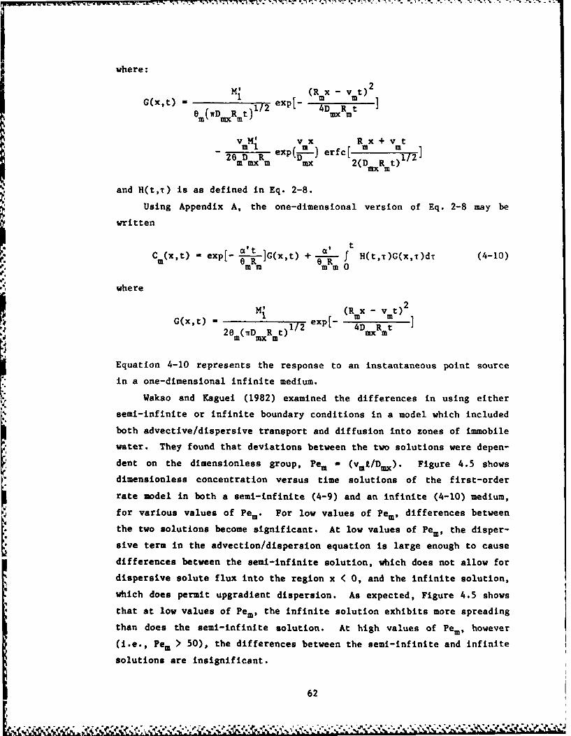
where:
H' (Rmx - vmt)2
G~~)- 1t ]G~xt)112 expl 4D R tem(wDmxRmt) mx m
vM vx Rx+vtm2 exp(D--m') erfc[ m m ]
2 mDmx m mx 2(D xRmt)
and H(t,r) is as defined in Eq. 2-8.
Using Appendix A, the one-dimensional version of Eq. 2-8 may be
written
C (xt) - exp[- .'! ]G(xt) + o f H(t,)G(x,)dT (4-10)- mRm mm0
where
MI, (R mx - V mt02_=172 exp[- 4D
2m( rDmx Rmt) mx m
Equation 4-10 represents the response to an instantaneous point source
in a one-dimensional infinite medium.
Wakao and Kaguei (1982) examined the differences in using either
semi-infinite or infinite boundary conditions in a model which included
both advective/dispersive transport and diffusion into zones of immobile
water. They found that deviations between the two solutions were depen-
dent on the dimensionless group, Pem - (vmt/Dmx). Figure 4.5 shows
dimensionless concentration versus time solutions of the first-order
rate model in both a semi-infinite (4-9) and an infinite (4-10) medium,
for various values of Pem. For low values of Pem, differences between
the two solutions become significant. At low values of Pem, the disper-
sive term in the advection/dispersion equation is large enough to cause
differences between the semi-infinite solution, which does not allow for
dispersive solute flux into the region x < 0, and the infinite solution,
which does permit upgradient dispersion. As expected, Figure 4.5 shows
that at low values of Pem, the infinite solution exhibits more spreading
than does the semi-infinite solution. At high values of Pem, however
(i.e., Pe > 50), the differences between the semi-infinite and infinite
solutions are insignificant.
62

0.5
Peru 100z_o0.4 _0 ------ Semi-infinite
- Infinitez
00.3 -
w
-0 Pe.lz5 "
zoN Pe. =I /
z0.1-
00 1.0 2.0
DIMENSIONLESS TIME, "
Figure 4.5. Comparison of semi-infinite and infinite solutions to thefirst-order rate model: 0.90, a 0.004 d1 , v/Z0.02 d-1, and R. = Rim = 1.0.
The solution of the spherical diffusion model in a one-dimensional
semi-infinite medium is found by a straightforward application of the
methods of Rasmuson and Neretnieks (1980) and van Genuchten et al.
(1984). The solution, for an instantaneous point source, is:
4MjDeexp(V0X/2Dx) /exp - R 12
Go 24,Dexp xrbD 1/2_
(C- z)~t ms om - x) xZ)
1/2 2 1/2
where Z and Zm are defined in Eq. 2-12.
p
63
• " .,, ,." = % % . ". . , .. . .- o .- - , ,- q - . . , . . , . . . . -. . .. . . *. °, ' o% ' % ., ' .' ,'*..,"-.e

Using the methods of Appendix B, the one-dimensional version of
Eq. 2-12 may be written:
2MID exp(vm x/2D )C M(x,t) 2 m /mm ~ m~2 1Dx~ /2
e mR im b D xRm)
. R , 1/2
00Ip - xIzp 2 1/2x P[ D) 2][ 2t R ! xZ
2D' 2 t R 1/2+ ~ Z(R\ _ XZ XdX(-2m b2 Q d) (4-12)
where, again, Z p and Zm are defined in Eq. 2-12. Equation 4-12
represents the response to an instantaneous point source in a one-
dimensional infinite medium.
Figure 4.6 compares dimensionless concentration versus time
solutions of the spherical diffusion model in both a semi-infinite
(4-11) and an infinite (4-12) medium, for various values of Pem. The
results are quite similar to the results obtained using the first-order
rate model. At high values of Pem, the difference between the semi-
infinite and infinite solutions decreases.
CONCLUSIONS
In this chapter, the equivalence between the local equilibrium,
first-order rate, and geometrical diffusion models was evaluated. It was
shown that the equivalence relationships derived using one-dimensional
model formulations of the various models are also applicable in three
dimensions, and that breakthrough responses simulated using the one- and
three-dimensional models show a similar dependence on input parameter
values.
Use of field breakthrough (temporal) data to differentiate between
the three types of models does not seem feasible, though spatial moment
data may be useful in differentiating between the equilibrium and non-
equilibrium model formulations.
64
.. X

0.5
Pe, I00
0.4- Semi-infinite0- Infinite
4 -I-z 0.3-Il
0 Pem:50z0
0.2-
_JZ Pe.: I10 0.1- /* 'r)
00 1.0 2.0DIMENSIONLESS TIME , .
Figure 4.6. Comparison of semi-infinite and infinite solutions to thespherical dif fusion model- 4 - 0.90, Be/b2 0.004v/X - 0.02 d- , and R. - Rim - 1.0.
It was also demonstrated that the solutions for semi-infinite and
infinite boundary conditions are similar at large values of the Peclet
number. This is convenient, since the infinite solution is simpler and
obtained in a more straightforward manner than the semi-infinite solu-
tion.
65

CHAPTER 5
APPLICATION TO THE INTERPRETATION OF DATA FROM A
LARGE-SCALE TRANSPORT EXPERIMENT UNDER NATURAL CONDITIONS
The discussion thus far has concentrated on the development and
analysis of three-dimensional physical nonequilibrium models. In this
chapter, spatial and temporal data obtained from a large-scale transport
experiment will be interpreted using such models. The physical nonequi-
librium models, with parameters obtained from direct measurement, liter-
ature correlations, and laboratory experiments, will be used in an
attempt to simulate the spatial and temporal behavior of the solute
distributions which were observed over the course of the experiment. In
addition, the complementarity of the results from spatial and temporal
sampling will be assessed in two ways. First, a direct comparison will
be made of spatial and temporal results obtained at comparable time/dis-
tance scales. Second, equilibrium and physical nonequilibrium model
parameters obtained from spatial sampling will be used to simulate
temporal response data. Finally, a brief review will be made of various
alternative models which may be used in interpreting the field results.
This review will include an examination of the spatial moment behavior
predicted by some of the alternative models, a subject that previously
has not been evaluated systematically.
PROJECT BACKGROUND
A large-scale, long-term field experiment to study natural gradient
transport of solutes in groundwater was conducted by a group of investi-
gators from Stanford University and the University of Waterloo, at a
site in Borden, Ontario (Mackay et al., 1986; Freyberg, 1986; Roberts et
al., 1986). Well-defined initial conditions were achieved by injecting
approximately 12 m3 of a solution containing known masses of two inor--
ganic tracers (chloride and bromide) and five halogenated organic
compounds (bromoform, carbon tetrachloride, tetrachloroethylene, 1,2-
dichlorobenzene, and hexachloroethane). The transport of the organic
solutes was monitored over a two-year period with a dense, three-
dimensional array of more than 4000 sampling points. Figure 5.1 depicts
the sampling network.
66

'~~~~0 '1 GO t7 Ir ''I. .
A"
100-
so
4.. 4 4 4 4
40 -
2 0 . . . *
+o-++. *Multilevel SoMlers
::: ..: • ijcto n W ells0o t,': i No Time Series Monitoring Points
0 20 40 so e0
Y (M)
0oAA
-2 .' .' : : . . ...... . . .. • . o
2 !
. .. .. 4.. .. . . . "
0 20 ""
D4s4nce e
Figure 5.1. Locations of multilevel sampling and injection els as of
anuary 1986: a) Plan vie, and b) Approximate vertical
distribution of sampling points ()projected onto cross
section AAI (vertical exaggeration =4.6).
67
4.. 4 4 4 4..
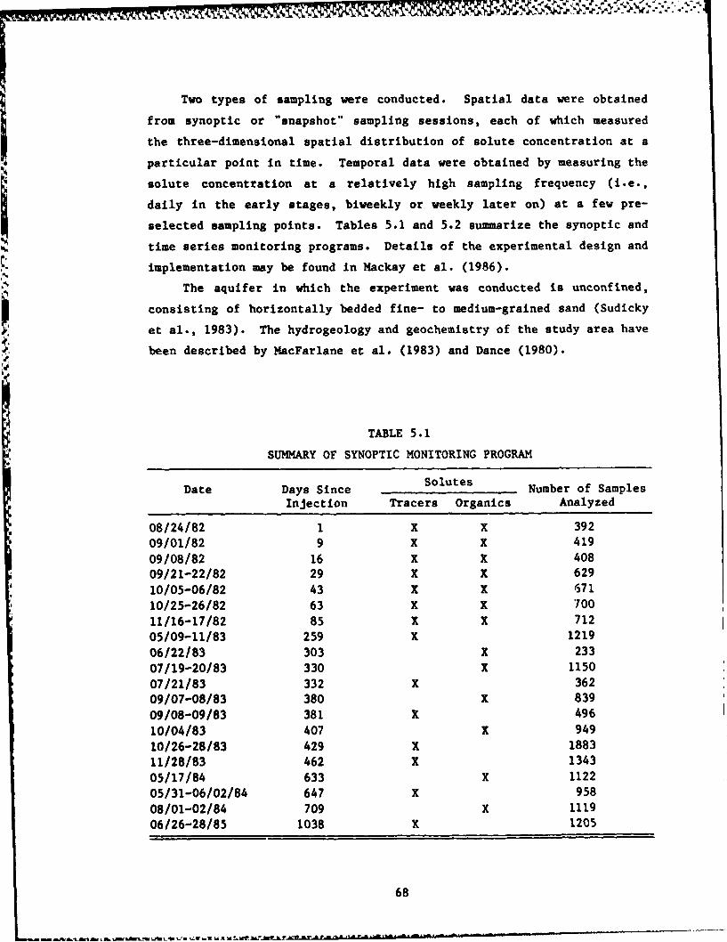
Two types of sampling were conducted. Spatial data were obtained
from synoptic or "snapshot" sampling sessions, each of which measuredI the three-dimensional spatial distribution of solute concentration at aparticular point in time. Temporal data were obtained by measuring thesolute concentration at a relatively high sampling frequency (i.e.,
daily in the early stages, biweekly or weekly later on) at a few pre-
selected sampling points. Tables 5.1 and 5.2 summarize the synoptic and
time series monitoring programs. Details of the experimental design and
implementation may be found in Mackay et al. (1986).
The aquifer in which the experiment was conducted is unconfined,
consisting of horizontally bedded fine- to medium-grained sand (Sudickyp et al., 1983). The hydrogeology and geochemistry of the study area have
been described by MacFarlane et al. (1983) and Dance (1980).
TABLE 5.1
SUMMARY OF SYNOPTIC MONITORING PROGRAM
Date Days Since Solutes Number of SamplesInjection Tracers Organics Analyzed
08/ 24/82 1 X X 39209/01/82 9 X X 41909/08/82 16 X X 40809/21-22/82 29 X X 62910/05-06/82 43 X X 671
10/25-26/ 82 63 K X 700
11/16-17/82 85 X X 71205/09-11/83 259 X 1219
06/22/83 303 K 23307/19-20/83 330 X 1150
07/21/83 332 X 36209/07-08/83 380 X 83909/08-09/83 381 x 496
10/04/83 407 X 94910/26-28/83 429 x 188311/28/83 462 X 134305/17/84 633 x 112205/31-06/02/84 647 K 958
08/01-02/84 709 X 1119
06/26-28/85 1038 X 1205
68

TABLE 5.2
SUMMARY OF TIME SERIES MONITORING PROGRAM
Sample Point (x,yz) Number of Samples(m) Duration Collected as of 1/1/86
Near- 2.5, 0.0, -3.20 Aug. 82 - Dec. 83 188Feld 2.5, 1.25, -3.62 Aug. 82 - Dec. 83 188
5.0, 0.0, -3.26 Aug. 82 - Dec. 83 183
10.0, 4.6, -3.88 Nov. 83 - Jun. 85 45Mid- 10.0, 4.6, -4.48 Nov. 83 - Jun. 85 27
Field 13.1, 4.05, -3.42 Jul. 84 - Jun. 85 3213.1, 4.05, -3.72 Jul. 84 - Jun. 85 31
18.0, 9.0, -4.13 Mar. 83 - Jun. 85 119Far- 18.0, 9.0, -4.73 Mar. 83 - Jun. 85 121
Field 21.0, 9.0, -4.17 Mar. 83 - Jun. 85 11721.0, 9.0, -4.77 Mar. 83 - Jun. 85 11724.0, 9.0, -4.76 Mar. 83 - Nov. 83 78
Time Series Data
Concentration responses at each of the twelve high frequency sampl-
ing points are shown in Appendix E. Chloride data are not depicted, in
the interest of clarity, since the chloride and bromide observations are
nearly indistinguishable (Freyberg, 1986). For the purpose of this
study, 1,2-dichlorobenzene and hexachloroethane data have also been
omitted. As discussed in Roberts et al. (1986), both of these compounds
behaved anomalously. Hexachloroethane concentrations declined to non-
quantifiable levels by the end of the first three months of the experi-
ment, and the concentration of 1,2-dichlorobenzene declined precipitously
at one of the three near-field sampling wells and was never found in
significant levels thereafter. Significant concentration levels of
1,2-dichlorobenzene were not seen at either of the other two near-field
wells. A full discussion of the near-field, early-time behavior of
these two compounds may be found in Roberts et al. (1986). This study
will focus on those compounds that remained at significant concentration
levels after the first three months of monitoring.
Appendix E also shows that of the four solutes being considered,
every solute is not seen at every sampling point. The four mid-field
wells were sampled specifically for tetrachloroethylene. Bromide and
the two faster moving organics, carbon tetrachloride and bromoform, had
largely passed by these wells before sampling commenced. At the five
69

far-field wells, tetrachloroethylene had yet to arrive upon conclusion
of the experiment. At the most distant well, only bromide was seen,
since sampling at this well was terminated prior to the arrival of the
organic solutes.
Synoptic Data
Freyberg (1986) described how the synoptic concentration data were
used to obtain estimates of the spatial moments of the solute plume dis-
tributions. Freyberg (1986) and Roberts et al. (1986) present estimates
of the zeroth and first moments for the inorganic and organic plumes,
respectively. Freyberg (1986) also presents estimates of the second
moment for the inorganic plumes. Following his methods, the organic
plumes' second moment estimates were calculated as well (Freyberg,
1985). In this work, estimates of the second moment are presented as2 and y, the principal values of the spatial covariance tensor.
Freyberg (1986) noted that the vertical components of the spatial
covariance tensor could not be distinguished from sampling noise, and
that the vertical thickness of the tracer plumes remained essentially
constant over the course of the experiment. Therefore, the principal
vertical component of the covariance tensor, azz , has not been consid-
ered and will be assumed to be negligible.
Comparison of Time Series and Synoptic Results
Roberts et al. (1986) demonstrated that the results of time series
sampling of the near-field wells (x < 5 m) were qualitatively consistent
with synoptic sampling results. In this section, far-field (x > 15 m)
time series sampling results for bromoform and carbon tetrachloride are
presented, and compared with synoptic sampling results, to further
demonstrate the complementarity of spatial and temporal transport behav-
ior. The comparison is made in terms of the retardation factor, which
is calculated using temporal or spatial first moment estimates, and the
relative mass ratio, which is obtained from temporal or spatial zeroth
moment estimates. The following definitions are used:
1. Retardation factors are defined by Eqs. 3-55a and 3-55c,
based on temporal and spatial first moment estimates,
respectively.
70
- ... ..... -. ..... ,... - . *.. '. ..- €' ... - ,.. ' "... .. ,.-..... -

2. Relative mass is def ined as the total solute mass calcu-
lated from the temporal or spatial zeroth moment estimate,
normalized by the total solute mass initially injected
into the aquifer. The relative mass ratio is the rela-
tive mass of a retarded solute divided by the relative
mass of the conservative tracer. The relative mass cal-
culated from the temporal zeroth moment is proportional
to the area under the breakthrough response curve. The
relative mass calculated from the spatial zeroti moment
is proportional to the product of the zeroth moment and
the retardation factor. As noted above, for this analy-
sis, the retardation factor at a particular synoptic
sampling time is obtained from Eq. 3-55c. The reason the
mass calculated from the spatial moment is proportional
to the retardation factor while the mass calculated from
the temporal moment is not, goes back to the discussion
in Chapter 3. When determining the spatial moment at an
instant in time, only the aqueous solute concentration is
measured. The sorbed solute must be accounted for, in
this instance, by use of the retardation factor. On the
other hand, when determining the temporal zeroth moment,
all the solute passing by a particular sampling point is
accounted for in the breakthrough response curve.
In order to graphically compare spatial and temporal behavior, it
is useful to plot the two types of results on the same scale. Spatial
data are obtained at particular sampling times. The sampling distances
at which temporal data are obtained may be converted to equivalent time
values. For this analysis, the first moment of the breakthrough re-
sponse curve of the solute of interest at a sampling point is defined as
the equivalent time for that point.
Figures 5.2 and 5.3 depict the relative mass ratios and the retar-
dation factors for bromoform and carbon tetrachloride calculated from
temporal and spatial moment estimates. For bromoform, the decrease in
mass and the Increase in the retardation factor which was found by an
examination of the spatial data (Roberts et al., 1986) is also clearly
seen by comparing near- and far-field temporal results. The obviuus
disappearance of bromoform (Figure 5.2) was attributed to transformation
71i

21.9 -
1.8
1.7-1.6 - 0 Estimated from spatial data1.51.4 ++ Estimated from temporal datao1.3-
0, 1.2-
I 1.1- +a 1I0o2 1 - a
V 0.9- A.
0.8 o16 0.7 -
0.6-0.5-0.4- +
0.3-0.2-0.1 -
0 I
0 200 400 600 goo
TIME (days)
3
2.8- +
2.6- 0
2.4-
2.2
2o00+1.8- Of
c 1.6-o +
1.4- B.VI. [
1.2-
a- 1 -
0.5- 0 Estimated from spatial data
0.6- + Estimated from temporal data
0.4-
0.2-0-I I I I I
0 200 400 600 800
TIME (days)
Figure 5.2. Comparison of the bromoform plume behavior determined fromspatial and temporal data: a) Relative mass ratio, andb) Retardation factor versus time.
72
.~~~~~ ~~~~~~~ .... ... . .......... +;+.. ,.;,,,l,,,,;+;,, .

21.9-1.8-
1.71.61.5 +
1.44 1.3 -n 1.2 +
S 1.1 .
0 +
o 1 0 A.* 0.9 0
4- 0.8 +
" 0.7 -0.6
0.50.4 - Estimated from spatial data +
0.30.2 - + Estimated from temporal data
0.10 . I I I
0 200 400 600 800
TIME (days)
3
2.8 + +
2.6-
2.4 +
2.2 a2
0 D.o 1.8 +
13C 1.6 +
.2 [B.o 1.4
1.21 -1
0.8 a Estimated from spatial data Q
0.6 - + Estimated from temporal data
0.4-
0.2-
0 I I I !
0 200 400 600 800
TIME (days)
Figure 5.3. Comparison of the carbon tetrachloride plume behaviordetermined from spatial and temporal data: a) Relativemass ratio, and b) Retardation factor versus time.
73
U ~ ~ j* U~. ~. ~

by Roberts et al. (1986). More variability is evident in the calcula-
tions of the relative mass for carbon tetrachloride, though again, the
increase in the retardation factor over the course of the experiment is
evident. The variability of the relative mass ratios obtained from the
temporal data may reflect local variations in aquifer properties along
the flow paths to the individual sampling points (Roberts et al., 1986).
Nevertheless, there is good general agreement between the results of the
spatial and temporal analyses.
MODEL APPLICATION
One goal of modeling is to predict real behavior using indepen-
dently obtained parameter values. In this section, an attempt is made
to predict zeroth and first spatial moment behavior using first-order
rate model parameters equivalent to the spherical and layered diffusion
model parameters. Model parameter values are estimated based on direct
measurement, literature correlations, and soil adsorption isotherms
measured in the laboratory.
Spherical Diffusion Model
Based on the approximately spherical shape of the aquifer material,
it is reasonable to assume solute diffusion into spherical grains may be
influencing transport. Table 5.3 lists parameter values for use in a
spherical diffusion model. The parameters in Table 5.3 were obtained
independently of the experimental data. The mass of each solute ini-
tially injected into the aquifer (Mi) was known (Mackay et al., 1986).
Values for bulk density (p), and total porosity (e) were obtained by
direct measurement (Mackay et al., 1986) as was the range of median
grain sizes (b) (O'Hannesin, 1981). The value for the pore water
velocity (vo ) was based on estimates of hydraulic conductivity and
hydraulic gradient (Mackay et al., 1986). The ratio of mobile to total
water content (*) was calculated using the following expression:
(1 - a) (5-1)
where ca is the intragranular porosity. Intragranular porosity was
measured by mercury porosimetry (Demond, 1984). The distribution coeffi-
cients (Kd ) for the various organic compounds and Borden aquifer material
74
- 7-.

TABLE 5.3
PARAMETER VALUES FOR USE IN A SPHERICAL DIFFUSION MODEL
Bulk soil density (p) 1.81 g/cm 3
Total porosity (e) 0.33
Intraparticle porosity (ca) 0.01Ratio of mobile to total water content ( ) 0.979
Pore water velocity (vo) 0.079 m/dFraction of "mobile" sorption sites (f) 0.0
Median grain radius (b) 0.035-0.35 mm
Carbon Tetra-
Bromo- Tetra- chloro-Bromide form chloride ethylene
Distribution coeff.
(K cm3/g 0.0 0.17 0.17 0.48(d), c
Mass of injectedsolute (M), g 3,870 0.38 0.37 0.36
Liquid diffusion 4coeff. (DO), m2/d 1.74x10 7.17xl0- 5 7.34xi0 - 5 6.83x10- 5
Effective intraparticlediffusion coeff.(D'). m2/d 1.74x0 - 6 7.17×1- 7 7.34x0 - 7 6.8340-7
Equivalent first-orderrate constant (a'),d- 1 1.44-144 0.594-59.4 0.608-60.8 0.566-56.6
were measured by Curtis et al. (1986) in a series of batch sorption ex-
periments. Bromide, the inorganic tracer, is assumed to be nonsorbing.
The liquid diffusion coefficients (DO ) for the organic compounds were
estimated using the Wilke and Chang (1955) correlation. The liquid
diffusion coefficient for bromide was calculated using a method de-
scribed by Cussler (1984) for estimating the diffusion coefficient of
electrolytes. Since intraparticle diffusion is likely to be hindered by
the interaction of the solute and the sorbent grain, the effective
intraparticle diffusion coefficient (DI) is some fraction of the liquid
diffusion coefficient. Defining tortuosity (X) such that:
DO
1D - (5-2)e X
Wakao and Smith (1962) proposed:
IX C
a
75

Given the measured value of ea of 0.01, X 100. Equation 5-2 was used
to calculate the effective intraparticle diffusion coefficients for the
compounds being considered. Finally, a value for f, the fraction of
sorption sites adjacent to regions of mobile water is required for model
input. Nkedi-Kizza et al. (1982) assumed that for an aggregated soil,
virtually all the sorption occurs within the aggregate, so that there
are no sorption sites in direct contact with mobile water. Following
Nkedi-Kizza et al. (1982), it will be assumed that sorption occurseither within the aquifer material grains or within aggregates, so that
f - 0.0 for this model.
It is now possible to apply the moment analysis formulae of Table
4.1 to obtain first-order rate constants (a') equivalent to the spheri-
cal diffusion rates which can be calculated using the values of De, b,
*, and e in Table 5.3. This conversion to a first-order rate model is
chosen because of the convenience and computational efficiency of the
first-order rate model as compared to the diffusion models. In Chap-
* ter 4, it was shown that simulations obtained from each of the two model
types are quite similar, and probably indistinguishable considering the
accuracy of the experimental data and the accuracy with which the input
parameters are estimated. The range in values for a' is due to the
range in median grain sizes.
Before using the parameter values estimated above in the first-
order rate model, and comparing simulations with experimental data, it
is useful to discuss the relevance of the boundary and initial condi-
tions assumed in the model to the experimental conditions. The assump-
tion of infinite boundary conditions weould seem applicable in describing
the experimental conditions at Borden, in which the medium is unbounded
upgradient from the point of introduction, as well as downgradient from
the observation points. In any event, as was discussed in Chapter 4,
except for observation points close to the point of solute introduction,
the impact of boundary conditions on model predictions is small.
As was noted in Chapter 3, the assumption that no mass is initially
associated with the immobile region has a large effect on the mobile
region plume mass and velocity behavior. A related assumption is that
water which is obtained from the sampling wells is mobile water. The
former assumption implies, and the latter states, that water which is
injected into the aquifer by the injection system, or withdrawn from the
76

aquifer by the sampling system, is mobile water. Conceptually, these
assumptions seem reasonable. If it is assumed that regions of immobile
water do indeed exist in the Borden aquifer (within dead-end pores or
* zones of low permeability, for example), it follows that during injec-
tion or extraction, mobile water will be preferentially displaced. In
light of this preferential displacement, the initial condition assump-
tion and the assumption regarding the sampling water appear reasonable.
Therefore, in the following discussion, the moments calculated from the
spatial data will be assumed to be mobile region plume moments.
Figures 5.4 through 5.7 compare the mass in solution and first
spatial moments of the four mobile region solute plumes (Freyberg, 1986;
Roberts et al., 1986) with the moments simulated using the first-order
rate model. The Table 5.3 parameter values were used in the model.
Also shown in Figures 5.4 through 5.7 are the moments simulated using
the local equilibrium model. The local equilibrium model simulations
use the values of vo, m5, p, e, and Kd from Table 5.3, and implicitly
assume * - f= 1 (i.e., all water is mobile water). As these figures
show, the local equilibrium model and the physical nonequilibrium model
produce virtually identical results for the parameters used. These
results indicate that, based on the assumed diffusion coefficients and
grain sizes, for the time scale considered, local equilibrium is a valid
assumption. In particular, notice that varying the first-order rate
constant over two orders of magnitude has no effect on the results. The
reason for this insensitivity to the rate constant is that even for the
minimum value of the rate constant, local equilibrium is valid. There-
fore, increasing the rate constant has no effect on the %imulations.
Note, though, that the qualitative fit of the models to the data is
poor. The mass loss and the deceleration of the solute plumes which was
observed experimentally is not simulated by the models. One way to
simulate the observed spatial moment behavior is to adjust the diffusion
rate constant. Either a tenfold increase in the maximum median grain
size (from b - 0.35 mm to b - 3.5 mm, while holding De' constant) or
a one-hundredfold decrease in the effective intraparticle diffusion
coefficient (while holding b - 0.35 -m constant) will lead to a one-
hundredfold decrease in the minimum rate constant. Figures 5.8 through
5.11 compare the simulations of the first-order rate model using
this decreased rate constant with the experimental observations. As the
77

AD-RI71 256 THREE-DIMENSIONAL ANALYTICAL MODELING OF 2/2DIFFUSION-LIMITED SOLUTE TRANSPORT(U) AIR FORCE INST OFTECH MRIGHT-PATTERSON AFS ON M N GOLTZ JUL 86
UNCLASSIFIED AFIT/Cl/NR-86-131D F/O 8/8 NL
smhmhhhmmhhhu

1111 10 W! 12 .2
111L25 111114 EL
MICROCOPY RESOLUTION TEST CHARTNATIONAL BUREAU Of STANDARDS 1963-A

0 00 0
4- 0
+0+ +4
03 03 Estimated from data o A
1) + Equilibrium model
2- - Nenequilib model (low rate)
A Nonequilib model (high rate)
1
0 0.2 0.4 0.8 0.6 1SThousands)IQE (days)
90 - _ _ _ _ _ _ _ _ _ _ _ _ _ _ _ _ _ _ _ _ _ _ _ _ _ _ _ _
13 Estimated from data0
10 + Equilibrium model
70- -Nonequilib model (low rats)
A Nonequilib model (high rote)
Z 50-Lai
Z 40- B.
G 30-
10
00 0.2 0.4 0.6 0.8 1
Figure 5.4. Comparison of the bromide mobile region plume: a) Mass insolution, and b) First spatial moment, estimated from syn-optic data and simulated using an equilibrium and a first-order rate model equivalent to a spherical diffusion model.
78

0.4a Estimated from data
0.35- + Equilibrium model
- Nonequllb model (low rate)0.3- a
o A Nonequilib model (high rate)
0.25-
In 0.2A.
0.15
a
0.1 - a
0.05-13 a
0 I I I
0 200 400 600 800
TIME (days)
50-
0 Estimated from data
40- + Equilibrium model
- Nonequilib model (low rate)E
30 A Nonequilib model (high rate)z
20 "
10-
10
0 200 400 600 800
TIME (days)
Figure 5.5. Comparison of the bromoform mobile region plume: a) Massin solution, and b) First spatial moment, estimated fromsynoptic data and simulated using an equilibrium and afirst-order rate model equivalent to a spherical diffusionmodel.
79
Ln1

0.4
o Estimated from data
0.35- a + Equllibrium model
- Nonequilib model (low rate)0.3- 0 A Nonequilib model (high rate)
0.25 -D
2[132 A.
0.15 -
0.1 -
0.05-
0 1 I I I I
0 200 400 600 800
TIME (day.)
50 .
0 Estimated from data
40- + Equilibrium model
-Nonequllib model (low rate)E
30- A Nonequilib model (high rate)
z
2 20-W0
200
10-
0-0 200 400 600 800
TIME (days)
Figure 5.6. Comparison of the carbon tetrachloride mobile region plume:a) Mass in solution, and b) First spatial moment, estimatedfrom synoptic data and simulated using an equilibrium and afirst-order rate model equivalent to a spherical diffusionmodel.
8o
.)w

0.2-0.19 a Estimated from data0.18 + Equilibrium model
0.17 a0.16 - Nonequilib model (low rote)
0.15- a Nonequlib model (high rate)
0.14 -
0.13
0.12
0.11
0.09
0.08A
0.07
0.06-
0.05-
0.04-
0.03-
0.02
0.010I I I I I I
0 200 400 600 600
TIME (days)
26,,
24-
22 0 Estimated 1rom data
20- + Equilibrium model
1 - Nonequilib model (low rate)
%E 16- A Nonequilib model (high rote)I-zw 14-
0 0=2 12- 12 B.
I--
6-
4-
0
0 200 400 600 800
TIME (days)
Figure 5.7. Comparison of the tetrachloroethylene mobile region plume:a) Mass in solution and b) First spatial moment, estimatedfrom synoptic data and simulated using an equilibrium and afirst-order rate model equivalent to a spherical diffusionmodel.
81

6-
4- 0
000 0. . . .
90
23 03 Estimated from data
70 --- Decreased rate constant simulation
q 0
0 0.2 0.4 0.6 0.81( Thousands)TIME (days)
souton an E)Mtsaia oetstimated from data
70 ti -drasead rasiconsat siulation -rdrraemoe
28
0%

0.4
0.35 0 Estimated from data
0.3 01- Decreased rate constant simulation
0.25
0.2 A.
1
0.150
0.1 0 0
0.05
0• ! II I I I I
0 200 400 600 800
TIME (days)
45
40 o Estimated from data
35 - Decreased rate constant simulation
30~E
z 252 B.
0 2I- 20
10015-
10
0'
0 200 400 600 800
TIME (days)
Figure 5.9. Comparison of the bromoform mobile region plume: a) Massin solution, and b) First spatial moment, estimated fromsynoptic data and simulated using a first-order rate modelequivalent to a spherical diffusion model, with a very lowrate constant (a' * 0.00594 d-1 ).
83
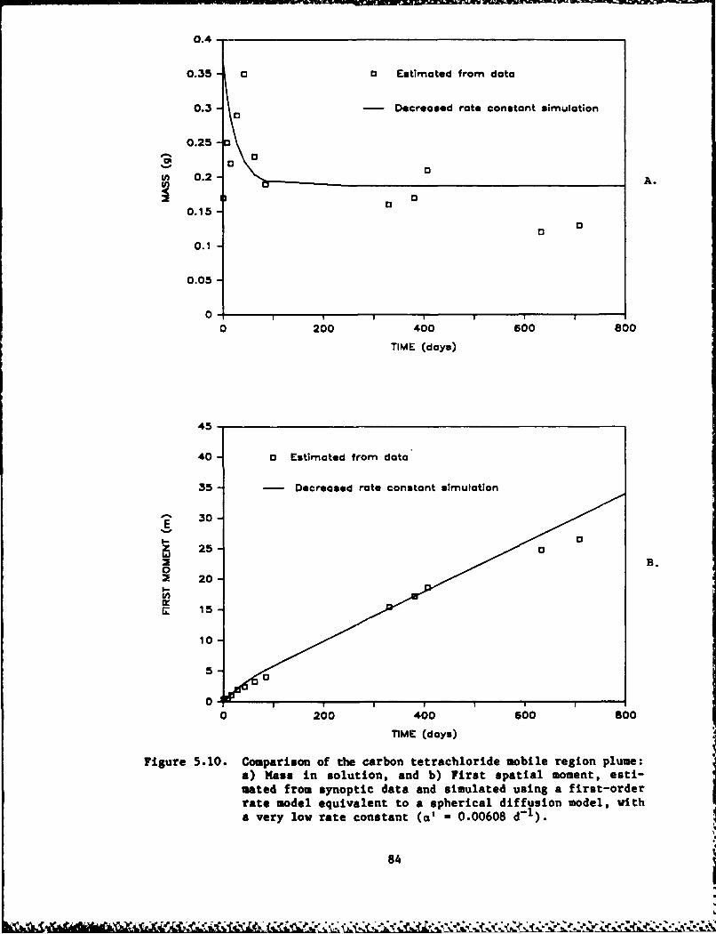
0.4 -
0.35 a Estimated from data
0.3- - Decreased rate constant simulation
0.25
m ~ 0.0-
S 0.2 A.
0,150.15
0.1
0.05
0- I I I I I I
0 200 400 600 00
TIME (days)
45
40- o Estimated from data
35- - Decreased rate constant simulation
30-E
z 25- 0W2 B.
2s 20-i-
,C- 15-
10-
0-
0 200 400 600 800
TIME (days)
Figure 5.10. Comparison of the carbon tetrachloride mobile region plume:a) Mass in solution, and b) First spatial moment, esti-mated from synoptic data and simulated using a first-orderrate model equivalent to a spherical diffusion model, witha very low rate constant (a' - 0.00608 d-1 ).
84

0.20.19-0.16 0 Estimated from data0.17 a0.16 - Decreased rate constant simulation
0.15 a0.14 a0.130.12
0.10.09 .0.08 o
0.07 13
0.060.050.040.030.020.01
0- I I I I I
0 200 400 600 800
TIME (days)
30
28- a Estimated from data
26-
24- Decreased rate constant simulation
22-
20-
Is-
20 14- B.2 a
12-
10-
6-
4-2- Do
0 200 400 600 800
TIME (days)
Figure 5.11. Comparison of the tetrachloroethylene mobile region plume:a) Mass in solution, and b) First spatial moment, esti-mated from synoptic data and simulated using a first-orderrate model equivalent to a spherical diffusion model, witha very low rate constant (a' * 0.00566 d-1 ).
85

figures show, the salient characteristics of the data are simulated by
the model. The mass in mobile solution moment simulations demonstrate
good fits to the data, except in the case of bromoform. The model,
which predicts no mass loss of bromide over the course of the experi-
ment, is consistent with the data. The mass loss of carbon tetrachlo-
ride and tetrachloroethylene is simulated by the model. The observed
mass loss of bromoform, however, is significantly greater than model
predictions. This discrepancy may be due to the biotransformation of
bromoform, a possibility which was discussed by Roberts et al. (1986).
The observed deceleration of the organic plumes, and the constant veloc-
ity of the bromide plume are qualitatively simulated.
The only parameter which was adjusted to fit the model to the data
in Figures 5.8 through 5.11 was the rate constant describing solute
transfer into the regions of immobile water. The fitted value of this
rate constant is lOOx less than was calculated using literature correla-
tions and the maximum median grain size. However, this hundredfold dis-
crepancy is not entirely unrealistic. Hutzler et al. (1986), using a
similar spherical diffusion model to simulate soil column breakthrough
responses, found that grain sizes on the order of 7-20x greater than the
mean particle grain size were required to get a good fit of the model
simulations to the experimental data. This increase in grain size is
equivalent to a 49- to 400-fold decrease in the rate constants calcu-
lated using literature correlations. An alternate explanation is that
strongly hindered diffusion is occurring. Such hindered diffusion has
been reported in the literature. Roberts (1966) estimated that hexane
diffusivity in zeolite crystals was seven orders of magnitude less than
bulk diffusivity. Satterfield et al. (1973) found that, for solute
molecular diameters on the same order as sorbent pore diameters, liquid-
phase diffusivities of hydrocarbons were less than bulk diffusivity val-
ues by several orders of magnitude. Prasher and Ma (1977) cited other
studies where the reported diffusivity values for organic solutes in zeo-
lites were several orders of magnitude less than bulk diffusivity values.
In addition, Ball and Roberts' (1985) finding that the attainment of
equilibrium in batch sorption studies measuring tetrachloroethylene
uptake by Borden aquifer material required at least several months also
supports the hypothesis of strongly hindered diffusion within Borden
aquifer material.
86
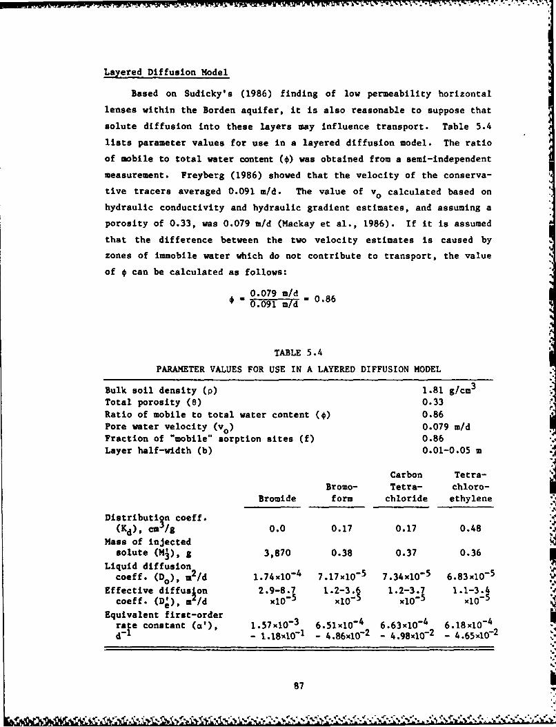
Layered Diffusion Model
Based on Sudicky's (1986) finding of low permeability horizontal
lenses within the Borden aquifer, it is also reasonable to suppose that
solute diffusion into these layers may influence transport. Table 5.4
lists parameter values for use in a layered diffusion model. The ratio
of mobile to total water content (f) was obtained from a semi-independent
measurement. Freyberg (1986) showed that the velocity of the conserva-
tive tracers averaged 0.091 m/d. The value of vo calculated based on
hydraulic conductivity and hydraulic gradient estimates, and assuming a
porosity of 0.33, was 0.079 m/d (Mackay et al., 1986). If it is assumed
that the difference between the two velocity estimates is caused by
zones of immobile water which do not contribute to transport, the value
of * can be calculated as follows:
0.079 m/d ' 0.860.091 mld
TABLE 5.4
PARAMETER VALUES FOR USE IN A LAYERED DIFFUSION MODEL
Bulk soil density (p) 1.81 g/cm3
Total porosity (0) 0.33Ratio of mobile to total water content (*) 0.86Pore water velocity (vo) 0.079 m/dFraction of "mobile" sorption sites (f) 0.86
Layer half-width (b) 0.01-0.05 m
Carbon Tetra-
Bromo- Tetra- chloro-Bromide form chloride ethylene
Distributin coeff.(Kd), cm /g 0.0 0.17 0.17 0.48
Mass of injectedsolute (Mi), g 3,870 0.38 0.37 0.36
Liquid diffusioncoeff. (Do), m2/d 1.74xi0- 4 7.17x10- 5 7.34xi0- 5 6.83xi0- 5
Effective diffus on 2.9-8.7 1.2-3. 1.2-3.7 1.1-3.4coeff. (D), mi/d x10 5 xlO - A5 l05x10 - 5
Equivalent first-orderrate constant (a'), 1.57xi0 - 6.51xi0 " 6.63i0-4 6.1810-4
d-1 _ 1.18xO-1 - 4.86x10⁻² - 4.98x1072 - 4.65x10²
87
- ,'W " .,s £ , ' " .: '= ' .. < , "
<.,: "':, ,, ,: .. , .. .

-.IL- ~
Of course, it must be realized that the value of vo represents a rough
estimate, so that the value of f calculated above should be viewed as a
gross approximation. However, for this exercise, which is meant to com-
pare qualitative characteristics of model simulations with the data,
such an approximation is adequate.
In the case of the layered model, diffusion is not assumed to be
intraparticle as it was for the spherical model, but rather interparti-
cle. For interparticle diffusion, values of X of 2-6 have been reported(Cussler, 1984). Thus, a range of D; may be calculated by dividing Dofor the various compounds by a factor of 2 to 6. The range of immobile
layer half-widths (b) was estimated based on the approximate dimensions
of the low permeability layers noted in Freyberg (1986). The fraction
of sorption sites adjacent to zones of mobile water (f) was approximated
assuming an equal distribution of sorption sites within the mobile and
immobile region volumes. Other parameter values are the same as those
used with the spherical diffusion model.
As with the spherical diffusion model, it is now possible to calcu-
late first-order rate constants (ax') equivalent to the diffusion model
rate constants which can be obtained from the Table 5.4 parameter
values. The range in the values of ai' is due to the range in the values
of Dand b, with the maximum a' calculated using the maximum value of
D' and the minimum value of b, and the minimum oil obtained using thee
Figures 5.12 through 5.15 compare the mass in solution and first
spatial moments calculated from the data of the four mobile region sol-
ute plumes with the mass in solution and first moments simulated using
the first-order rate model equivalent to the layered diffusion model.
Also shown are simulations using the local equilibrium model. As in
Figures 5.4 through 5.7 depicting the spherical diffusion model, the
differences between the nonequilibrium and the equilibrium simulations
do not appear significant, though at least for the low rate constant
simulations, the salient aspects of the solute behavior (mass loss and
deceleration) are seen. The magnitude of the simulated behavior, how-
ever, Is considerably less than that exhibited by the actual plumes.
The insignificance of the affect of the immobile region is largely due
to the assumption of the equal distribution of sorption sites between the
mobile and immobile water regions. Due to this assumption, the effect of
88

6-
a
4- 0
- 11
,,+ ,,4 + + ,4++U 4-4. +0
00
1:3 EEtimated from data
2 + Equlibrium model7 Nonequilb model (low rote)
A Nonequiib modl (high rate)
00.2 0.4 0.6 0.8 1S(Th ou a n d a.)
ME (days)
z 0-22 B.
0Estimated from data
80-
0-+ Equilibrium model /
70 - Nonequilib model (low rate)"-- II- 560 A Nonequilib model (high rate)
I-
,T 30-
20O
10
0 4
0 0.2 0.4 0.6 0.8 1(Thousands)TIME (days)
Figure 5.12. Comparison of the bromide mobile region plume: a) Mass insolution, and b) First spatial moment, estimated from syn-optic data and simulated using an equilibrium and a first-order rate model equivalent to a layered diffusion model.
89
%i

0.4o Estimated from data
0.35 + Equilibrium model
- Nonequilib model (low rate)
o A Nonequillb model (high rate)
0.25
(n 0.2 -4+ + + + ++ + ++ +
h&AA A B 0&
0.15
0.1 0
0.0513 0
0 200 400 600 800
TIME (days)
50
a Estimated from data
40 + Equilibrium model
Nonequilib model (low rate)E
30 A Nonequilib model (high rate)z
0 B.S 20
10-
.00 200 400 600 800
TIME (days)
Figure 5.13. Comparison of the bromoform mobile region plume: a) Massin solution, and b) First spatial moment, estimated fromsynoptic data and simulated using an equilibrium and afirst-order rate model equivalent to a layered diffusion
model.
90
S,,
- - - ~ - *°

0.4a Estimated from data
0.35 0 + Equilibrium model
- Nonequilib model (low rate)0.3 0 o A Nonequilib model (high rote)
0.25 -
in 0.2- d. + + + ++ + ++ + A.
0.15
0
0.1
0.05
0 200 400 600 800
TIME (days)
50
0 Estimated from data
40 + Equilibrium model
-Nonequilib model (low rate)
30 A Nonequilib model (high rate)zA
0B.
20
10 -
0
0 200 400 600 00
TIME (days)
Figure 5.14. Comparison of the carbon tetrachloride mobile region plume:a) Mass in solution and b) First spatial moment, estimatedfrom synoptic data and simulated using an equilibrium anda first-order rate model equivalent to a layered diffusionmodel.
91

0.2-0.19- a Estimated from data0.18 + Equilibrium model0.17- o0.16- - Nonequilib model (low rote)0.15 A Nonequllb model (high rate)0.14 -0.13 -
0.12-, 0.11 -(A 0.1 + ++++ +A
0.09
0.08 - -A
0.07-0.06-0.05-0.04 -
0.03 -
0.01 -
0 200 400 600 800
TIME (days)
24-
22- 0 Estimated from data
20- + Equilibrium model
18- - Nonequilib model (low rote)
16 A Nonequllib model (high rate)E
$-- 14 *lZ 03
12-
B.g 10-
8-
6-
4-
2 00
0-0 200 400 600 800
TIME (days)
Figure 5.15. Comparison of the tetrachioroethylene mobile region plume:a) Mass in solution and b) First spatial moment, estimatedfrom synoptic data and simulated using an equilibrium anda first-order rate model equivalent to a layered diffusionmodel.
92

the immobile region on solute transport .is limited, since relatively
little solute is associated with the immobile regions. Figures 5.16
through 5.19 demonstrate the impact of decreasing the value of f, thus
implying that more sorption sites are within regions of low permeabil-
ity. The assumption that low permeability regions, perhaps made up of
silty material, have a higher sorption capacity is not unreasonable,
though at the Borden site, there is no evidence correlating low hydrau-
lic conductivity with high distribution coefficients (Durant, 1986).
As Figures 5.16 through 5.19 show (using a value of f - 0.4 and a
value of the rate constant based on average values of D' and b), the
main characteristics of the data can be simulated, again with the excep-
tion of the decrease in bromoform mass (Figure 5.17), which is attrib-
uted to transformation.
If diffusion into low permeability lenses is occurring, and ifadvective transport through the lenses is faster than diffusive trans-
port into and out of the lenses, then advective transport would dominate
and the effect of diffusion into the lenses would be minor.
The concept of comparing advective and diffusive rates, introduced
in Chapter 3, may be used to determine the relative importance of advec-
tive and diffusive transport into low permeability lenses. Assume
lenses that are 0.06 m thick (b - 0.03 m), with hydraulic conductivity
two orders of magnitude less than the hydraulic conductivity of the
"mobile" regions. Therefore:
mo-4lens "- m 9.1 x 10 m/dVlens 100
and the advective rate constant for tetrachloroethylene transport in the
lenses would be:
vlens . (9.lxlO -4 m/d) 1.21 x 10- 3 d- 1
2b Rim 2(0.03 m)(12.5)
The diffusive rate constant would be:
3D' -5 2a e 2 3(l.71x10 m /d) . 4.56 x 10-
3 d- 1
Rim (12.5)(0.03 m) 2
using X - 4 to calculate D; from Do.
93

6
05-0
0
4- 00 0
3- A.
2 a Estimated from data
Increased immobile sorption site simulation
0
0I I I I I I|
0 0.2 0.4 0.6 0.8 1CThousandt)
IME (days)
90-
80 D Estimated from data70 - Increased immobile sorption site simulation
0 E so-
Ej 50-
00 40 B."
30
20
10
0-0 0.2 0.4 0.6 0.8 1
(ThousOnds)TME (days)
Figure 5.16. Comparison of the bromide mobile region plume: a) Mass insolution, and b) First spatial moment, estimated from syn-optic data and simulated using a first-order rate modelequivalent to a layered diffusion model, with high sorp-tion capacity within the imobile regions (f - 0.4).
94

0.4
0.35
0 Estimated from data0.3 0
00 - Increased Immobile sorption sete simulation
0.25 \0
W 0.2 A.
0.15
13
0.1 013
0.050 0
I I I I I I
0 200 400 600 800
TIME (days)
45
40 0 Estimated from data
35 - Increased immobile sorption site simulation
30
25-
B.20-
15
10
5
0*0 200 400 So0 800
TIME (days)
Figure 5.17. Comparison of the bromoform mobile region plume: a) Massin solution, and b) First spatial moment, estimated fromsynoptic data and simulated using a first-order rate modelequivalent to a layered diffusion model, with high sorp-tion capacity within the immobile regions (f - 0.4).
95

0.4
0.35- o 13 Estimated from data
0.3- - Increased immobile sorption site simulation
0.25-
U 0.2- A.
0.150
0.1 -
0.05-
0 -1 I I I 1 I
0 200 400 600 800
TIME (days)
45
40 0 Estimated from data
35 - Increased immobile sorption site simulation
30-E
z 25-
020 B.
I.-
15
10-
5
0-0 200 400 600 800
TIME (days)
Figure 5.18. Comparison of the carbon tetrachloride mobile region plume:a) Mass in solution, and b) First spatial moment, estimatedfrom synoptic data and simulated using a first-order ratemodel equivalent to a layered diffusion model, with highsorption capacity within the immobile regions (f = 0.4).
96

0.20.190.18 0 Estimated from data0.17 -
0.15 o0.14-0.13 0
0.12= 0.11W 0.1 A.
0.09-0.08 0 0
0.07 o0.060.050.04
0.030.020.01
0 I I I I II
0 200 400 600 800
TIME (days)
30
28 a Estimated from data
262 -Increased immobile sorption site simulation24-
22
20-
160 14 B.
0
12gn
r " 108 00 o
6
4
2
0 200 400 600 800
TIME (days)
Figure 5.19. Comparison of the tetrachloroethylene mobile region plume:a) Mass in solution, and b) First spatial moment, estimatedfrom synoptic data and simulated using a first-order ratemodel equivalent to a layered diffusion model, with highsorption capacity within the immobile regions (f - 0.4).
97

ICOPQ& Ix 1TL TX" ,1 ... 1 .CT AX.T '
Comparing the two rate constants, it is seen that for the assumed
parameter values, the diffusive rate constant is nearly four times
greater than the advective rate constant. This indicates that for rea-
sonable assumptions regarding lens characteristics (b > 0.03 m; lens
hydraulic conductivity 0.01 mobile region hydraulic conductivity), the
effect of diffusive transport would dominate the effect of advective
transport within the lenses. As the ratio of advective to diffusive
rate constants is independent of Rim, the dominance of diffusive trans-
port applies for all the compounds, since of all the solutes, tetra-
chloroethylene has the lowest estimated value of De.
Temporal Data Simulation
Another way of demonstrating the complementarity of spatial and
temporal transport behavior is to use the model parameters obtained in
the preceding analysis of the zeroth and first spatial moments to simu-
late temporal responses. The following discussion will use parameters
obtained assuming that layered diffusion dominates transport (Table 5.4
with f - 0.40), although either the layered or spherical diffusion model
assumptions could have been used for this exercise.
Values for longitudinal and transverse dispersion coefficients and
initial plume dimensions must be determined for use as model input
parameters. These parameters may be estimated from the second spatial
moment data. Figures 5.20 through 5.27 show Uix and y, the principal
values of the spatial covariance tensor, calculated for the four solutes
at each synoptic sampling time. Figures 5.20a through 5.27a compare
simulations of the local equilibrium model with principal values of the
covariance tensor. The values of the longitudinal and transverse dis-
persion coefficients (D and D;) and the initial plume length and width
(2L and 2M) were chosen to provide simultaneously a visual best fit to
the eight data sets. The other parameter values used in the equilibrium
model (vo, Kd, p and 0) were obtained in the preceding section. Simi-
larly, Figures 5.20b through 5.27b compare the second spatial moment data
with simulations of the first-order rate model. Recall that the first-
order rate constant used in the model was calculated to be equivalent to
the layered diffusion model rate parameter. As with the local equilib-
rium model, the longitudinal and transverse dispersion coefficients in
the mobile region (Dox and Dmy) and the initial plume dimensions (2L and
98

90.
60 t Estimated from data
7 Equilibrium model
70
60
0 r50-
A.
X 40
30 a
20 C]
10-
10 _ _ __ I I__ __
0 0.2 0.4 0.6 0.8 1(Thousands)
TIME (days)
90-0
80 a Estimated from data
- First-order rate model
70
60
E 5 0 0
eX 40 B.
30
20
10
0 1 ' I ' I 1 I
0 0.2 0.4 0.6 0.8 1(Thousands)
TIME (days)
Figure 5.20. Comparison of the bromide mobile region plume principalcomponent of the spatial covariance tensor in the longi-tudinal direction ) estimated from the synoptic dataand simulated by fitting the a) Equilibrium model, andb) First-order rate model to the estimates.
99

so
70-
60
50
0 Estimated from data
E 40 - Equilibrium model%MO A.*xt)30-
20D
10
0 . I I I I I
0 200 400 600 800
TIME (days)
80
70 1 Estimated from data
- First-order rate model
50
E%o40
x B.
0 30
20
20 100I 0
0 200 400 600 800
TIME (days)
Figure 5.21. Comparison of the bromoform mobile region plume principalcomponent of the spatial covariance tensor in the longi-tudinal direction (c~x) estimated from the synoptic dataand simulated by fitting the a) Equilibrium model, andb) First-order rate model to the estimates.
100

so -
70-
60-
50-
C4 0 Estimated from date
4, - Equilibrium model A.%00 A.
CV X 0t) 30 -
20
10
0 200 400 600 800
TIME (days)
70- 0 Estimated from data
- First-order rate model60-
50-04
x B.qt)x 0;
0 30-
10-
0 I II
0 200 400 600 800
TIME (days)
Figure 5.22. Comparison of the carbon tetrachloride mobile region plumeprincipal component of the spatial covariance tensor in thelongitudinal direction (a2 ) estimated from the synoptic
data and simulated by fitting the a) Equilibrium model,and b) First-order rate model to the estimates.
101

60
50
a Estimated from data
40 - Equilibrium model
E 3o- A.
%MOxC4 X20
*L100
0 200 400 600 800
TIME (days)
60
50 a Estimated from data
- First-order rate model
40
v 30 B.
x oaa20
010 -
0
0 200 400 600 800
TIME (days)
Figure 5.23. Comparison of the tetrachloroethylene mobile region plumeprincipal component of the spatial covariance tensor in thelongitudinal direction (xx) estimated from the synopticdata and simulated by fitting the a) Equilibrium model,and b) First-order rate model to the estimates.
102

2019117 -16 0 Estimoted from data 0
15 - Equilibrium model1413
o 1211
%tw~o A.
6. I 5
S 4
2
0 0.2 0.4 0.6 0.8 1(Thousands)[.
20- TIME (days)
19
17
71 6 -0 Estimated from data015 - First-order rate model14-
1344 12-
10 B.
0 a
3 05
2
0 0.2 0.4 0.6 0.5(Thousands)
TIME (days)
Figure 5.24. Comparison of the bromide mobile region plume principalcomponent of the satial covariance tensor in the trans-verse direction (oil ) estimated from the synoptic dataand simulated by fflting the a) Equilibrium model, andb) First-order rate model to the estimates.
103

10*
9 13 Estimated from data- Equilibrium model
7-
%woo A.4
3-
2-
1 C
0
0 200 400 S00 S0
TIME (days)
10*
9 - Estimated from date- Frst-ordor rote model
7-
£C4 8
B.
3-
2
0
O 200 400 600 800
TIME (days)
Figure 5.25. Comparison of the bromoform mobile region plume principalcomponent of the 8 atial covariance tensor in the trans-verse direction (al ) estimated from the synoptic dataand simulated by fi~?ing the a) Equilibrium model, andb) First-order rate model to the estimates.
104

10
9- a Estimated from dataEquilibrium model
8
7 0
6-
A.
40
3
2
1
0 , I I I I
0 200 400 600 800
TIME (days)
10
9 o Estimated from dataFirst-order rate model
: 8
7 -6-i 5 -
B.
3 0
2
0 200 400 600 800
TIME (days)
Figure 5.26. Comparison of the carbon tetrachloride mobile region plumeprincipal component of the spatial covariance tensor in thetransverse direction (o2 ) estimated from the synopticdata and simulated by fting the a) Equilibrium model,and b) First-order rate model to the estimates.
105

7 0 Estimated from data
- Equilibrium model
6
44 0
E4 -0 A.
C4 0
t) 3-
2
0
0 200 400 600 Soo
TIME (days)
7 0 Estimated from data- First-order rate model
6-
5-
4-
B.
3
2
0
0 I 1 1 ! 1 1 I
0 200 400 600 800
TIME (days)
Figure 5.27. Comparison of the tetrachloroethylene mobile region plumeprincipal component of the spatial covariance tensor in the
transverse direction (02 ) estimated from the synopticdata and simulated by fiMting the a) Equilibrium model,and b) First-order rate model to the estimates.
106
Law i ;%W,

2M) were adjusted to obtain simultaneously a visual best fit to the
eight data sets being considered. Other parameters used in the model
were obtained in the previous section (Table 5.4). A value of f - 0.4
was used to test whether parameters which have been shown to simulate
the spatial behavior can also simulate the temporal behavior. Table 5.5
lists the values for the dispersion coefficients and the initial plume
dimensions which will be used in the following analysis of the temporal
behavior.
TABLE 5.5
VALUES FOR DISPERSION COEFFICIENTS AND INITIAL PLUMEDIMENSIONS OBTAINED FROM SPATIAL SECOND MOMENT DATA
Local Equilibrium Model D - 0.04 m2/d- 0.008 m2 /d
yL -2.5 mM -2.0 m
First-Order Rate Model*
D x - 0.02 m2/dDmy - 0.008 m2/d
L - 2.5 mM - 2.0 m
*Equivalent to layered diffusion model.
6.
Using the parameter values in Tables 5.4 and 5.5, it is possible to
simulate both the temporal moments and the measured temporal responses
at particular sampling wells. Figures 5.28 through 5.31 compare zeroth
and first temporal moments estimated from the data with predictions of~equilibrium and nonequilibrium models. Moment estimates were obtained
by numerically evaluating the breakthrough response data at the various
sampling wells, depicted in Appendix E, using the formulae:
m o t - Cj (tj - t J 1 )
(5-3)n
C it i(tj - tJ_ 1)
Dl,t mOst
where C - the normalized concentration measured at time tj.
107

60 + a Data
+ Equilibrium model
50 * Nonequilib model
40 +
A.30 +
00
wN 20
0
0 4 a 12 16 20 24
WELL X-COORD ALONG LINE OF TRAVEL (m)
350 -
300- 0 Data
+ Equilibrium model2 0 Nonequilib model 0250 o
200-
02 150-0-
100
£ 0
0 4 a 12 is 20 24
WELL X-COORD ALONG LINE OF TRAVEL (m)
Figure 5.28. Comparison of bromide temporal moments estimated from thedata and predicted by equilibrium and nonequillbriummodels: a) Zeroth, and b) First moments.
108

70 -
510 +
0 Data
S 50- + Equilibrium model
a 0 .- onequii modelS 40- +
0 A.30- +
0
20 0
10 0
0 a 12 16 20 24WELL X-COORD ALONG LINE OF TRAVEL (in)
700
O Data
600- + Equilibrium model
* Nonequilib model
500 *
o 0
.. 400-
B.S300-
200-
04
0-0 4 a 12 16 20 24
WELL X-COORD ALONG LINE OF TRAVEL (mn)
Figure 5.29. Comparison of bromoform temporal moments estimated fromthe data and predicted by equilibrium and nonequilibriummodels: a) Zeroth, and b) First moments.
109
.. ............ e -

70-
o Data
60- + Equilibrium model
* Nonequilib model
a 50
- 40 +za0 A.0
30-
wN 20-
10-
0 I I I I I
0 4 a 12 16 20 24
WELL X-COORD ALONG LINE OF TRAVEL (m)
600-
500 0 Data
+ Equilibrium model 0
" 400 0 Nonequilib model0
300 B.2 B0
I 200
U
00
100 +
O- I I I I I I I I
0 4 a 12 16 20 24
WELL X-COORD ALONG LINE OF TRAVEL (m)
Figure 5.30. Comparison of carbon tetrachloride temporal moments esti-mated from the data and predicted by equilibrium and non-equilibrium models: a) Zeroth, and b) First moments.
110

70
60O
G
* 50 0 Date0 aV + Equilibrium model
z 40 o Nonequilib model
2 A.0
2 30-
0
N 20
10-
0
0 2 4
WELL X-COORD ALONG LINE OF TRAVEL (m)
300
280- a Data
260 ++ Equilibrium model a240
220 0 Nonequilib model
", 200
0 140o*0
120
0: 100-.G:-
80
2060
0 I I I
0 2 4
WELL X-COORD ALONG UNE OF TRAVEL (m)
Figure 5.31. Comparison of tetrachloroethylene temporal moments esti-mated from the data and predicted by equilibrium and non-equilibrium models: a) Zeroth, and b) First moments.
III111
5l

Model predictions were made using the equilibrium and nonequilib-
rium models to simulate breakthrough responses. The moments of these
responses were then evaluated using the same numerical technique that
had been applied to the data. In Chapter 3, Table 3.3, it was shown
that both equilibrium and nonequilibrium models have the same expression
for the zeroth temporal moment in terms of the model's parameters. Thus,
differences in the zeroth moment simulations of the two model types are
due to parameter differences, and not to model structure. Although
certain trends are evident, the zeroth moment data and simulations show
a fair amount of scatter. Both models simulate the low values of the
zeroth moment found at the sampling well located at x - 4.79 m. This
low value is observed because the sampling well is offset a considerable
distance from the center line of the plume. It is also apparent that
the zeroth moment data values for bromoform at the far-field wells are
considerably lower than the simulated values. This discrepancy may be
due to the possible biotransformation of bromoform, which was discussed
earlier in connection with the zeroth spatial moment results.
From Table 3.3 in Chapter 3, it was also found that the first tem-
poral moment calculated using the nonequilibrium models is equal to the
first temporal moment of the equilibrium model multiplied by a constant.
Again, therefore, any differences in the first temporal moment simula-
tions are due to parameter differences, rather than to differences in
model structure. Figures 5.28b through 5.31b show the first temporal
moment as a function of distance in the x direction. Reasonably good
agreement is found between simulated moments and moments calculated from
the data.
Judging from the zeroth and first temporal moment simulations,
there is little evidence for saying one model or the other is better at
describing the data, largely because both type models can be considered
"pseudo-equilibrium models" with respect to temporal moments. That is,
since the zeroth and first temporal moments calculated using the non-
equilibrium models are independent of the rate parameter, the zeroth and
first moments can be reproduced by an equivalent equilibrium model.
Figures 5.28 through 5.31 do indicate, ho!'ever, that the parameter val-
ues obtained from fitting the spatial moment data can be used to predict
the temporal moment data fairly well, for both equilibrium and nonequi-
librium models.
112

Another vay of examining the temporal data is to inspect the break-
through responses themselves, at various veils. Using one-dimensional
models, Goltz and Roberts (1986) shoved that the sharp breakthrough and
tailing exhibited by the near-field veil breakthrough response data vas
better simulated using nonequilibrium than equilibrium models. Figures
5.32 through 5.39 compare simulations of three-dimensional equilibrium
and first-order rate models vith the data. For each solute. two veils
vere chosen for comparison, one near-field veil and one far-field veil.
Figure 5.37, which compares simulations of the equilibrium and first-
order rate models with the near-field weil response data for bromoform,
also includes a layered diffusion model simulation. The similarity of
the first-order rate and layered diffusion model simulations provides
further evidence justifying the use of the first-order rate model to
approximate the more complex diffusion models.
As the temporal moments have already been discussed, the followinganalysis will concentrate on the general characteristics and form of thebreakthrough responses. The breakthrough responses simulated for the
four solutes at the far-field veils are fairly symmetric, with the non-
equilibrium model response exhibiting a bit more asymmetry than that of
the equilibrium model. It is interesting to note that for the bromide
simulated responses, the equilibrium model curve exhibits more spreading
and a lover peak value than that of the nonequilibrium model, whereas
for the organic simulations, the situation is reversed. The reason for
this behavior may be found by applying Eq. 3-66 to the nonequilibrium
model parameter values for the different solutes. Applying Eq. 3-66,
which calculates an equivalent dispersion coefficient (Deff), reveals
Deff for the bromide at the sampling veil to be less than Deff for the
organics. The value of Def f which is calculated using Eq. 3-66 is an
equilibrium model equivalent parameter which combines the effect of
dispersion in the mobile region with the effect of so-called "holdup
dispersion" (Koch and Brady, 1986). (Holdup dispersion describes a
spreading mechanism caused by solute diffusion into immobile regions.)
Owing to the sorption of the organic solutes within the immobile region,
the impact of holdup dispersion on the organic compounds' behavior is
more pronounced than the impact on the conservative tracer's behavior,
so the organic simulations exhibit relatively more spreading at the far-
field sampling points.
113

0.7 -
D
0.6- 3 Data 13
z x Equilibrium model00
P 0.5 - First-order rate model 13
I- 0z 0LJU.. 0.4-0 1z0 r
LA 0.3 0
N_j
xt 0.2-0 C
z l0.1
0
0 A
0 200 400
TIME (days)
Figure 5.32. Breakthrough response data and model predictions forbromide at a far-field veil (x - 21.0 In, y 9.0 m,z - -4.17 in).
0.15-
0.14 -0C Data
0.13 -x Equilibrium model x
0.12 - First-order rate model X Xz x2 0.11
0.1 -xz. x
L 0.09
Z 0.08-0
L)0.07 xx
N 0.06-
(0.05
o 0.04-z Q
0.03-
0.02 -xx
0.01 PbX
0 0.2 0.4 0.6 0.8(rThousands)
Figure 5.33. Breakthrough response data and model predictions forbromoforn at a far-field weil (x - 21.0 in, y -9.0 mn,z - -4.17 mn).
114

0.15.
0.14 0 Data
0.13 x Equilibrium model xxx
0.12 - First-order rate model 0] xz x xo 0.11 00 []3- 0.1 0
Z 0 ×,i 0.09Z 0.080
0.07-
N 0 .0 6 []
< 0.05O 0.04 xtY x
0.03 0 % []
0.02 x 0x C-9
0.01 -xxx,, i x
0 0.2 0.4 0.6 0.8Thousands)IME (days)
Figure 5.34. Breakthrough response data and model predictions forcarbon tetrachloride at a far-field well (x 21.0 m,y - 9.0 m, z - -4.17 m).
0.08
0 Data xx
0.07 x Equilibrium model x xx
- First-order rate model x x izo 0.06 x
0 xn- x0.05 0
Lu XC.-.)
z [ x0 0.04 x 00
[]Wx
oi 0.03
x 0x0 0.02 -x 0
x []
0.01 x
0 T __-il I I I I I Il I
0 0.2 0.4 0.6 0.8Thousands)IME (days)
Figure 5.35. Breakthrough response data and model predictions fortetrachloroethylene at a mid-field well (x - 13.1 m,
4.05 i, -3.72 w).
115

1 -
0.9 - 0 n Data
Rx x xx x Equilibrium model0.8- - First-order rate modelz
0 0.7- 1ItI- 0Ld 0.6-(AJ
z0 0.5- x
U 00N 0.4-4 : x x
: 0.3- o x0 0
0.2 - I x
0 X
0 .1 -
0 8B"' B 4U =& a malm-f
0 20 40 60 80 100
TIME (days)
Figure 5.36. Breakthrough response data and model predictions for
bromide at a near-field well (x - 2.5 m, y - 1.25 m,
z - -3.62 m).
0.9
0.8- 0 Data
z O2D x Equilibrium model
0 -3 First-order rate model< 0Zl 0.6- + Layered diffusion model
z++U 0.5z0
0.4- x +Xx x
x xN X x
< 0.3- x
0 + XZ 0 .2 3
0.1 - a E xxxxxO . 0 ,x ,, x
0
0 20 40 60 80 100 120 140 160 180 200
TIME (days)
Figure 5.37. Breakthrough response data and model predictions forbromoform at a near-field well (x = 2.5 m, y - 1.25 m,z = -3.62 m).
116
'd"d ./ -". /. " " . :i&-"s ". ". "A.",, ." '. -u -'. ... .'--,KJ.-" - "- " "&"' ."'" *"".'". - " " "

1*
0.9 3 Data
0.8 -0 x Equilibrium model
z - First-order rate model0 1
- 0.7 o ,
w 0.6
z
Nl 0.3 - X 6x
[] C] x×z xx
0. _X
Li 0 .14I I I x-1 I
0 0 x x
Figure 5.38. Breakthrough response data and model predictions for
carbon tetrachloride at a near-field veil (x - 2.5 m,y 0 1.25 m, z x -3.62 i).
0.6 - 0 x x x x x______________________
06
0.5 40 Data
Z 0.38. x Equilibrium model
cao te -First--order rate model0.4 - 13 0]0.4 - 0
z(J
z0 0.3a 0
L.J
N X XX XX
< 0.2 X x0 X
z x0
0.1 - I
0 10O0 200 300 400
TIME (days)
; Figure 5.39. Breakthrough response data and model predictions for4 Cetrachloroethylene at a near-field veil (x = 2.5 in,
* y = 1.25 in, z = -3.62 in).
4
, 117
.. ... • x x .

Examination of the near-field responses seems to confirm Goltz and
Roberts' (1986) conclusion that the characteristically sharp break-
through and tailing of the breakthrough response data are better simu-
lated with the nonequilibrium models. On the other hand, in the far
field neither model type offers a significant advantage over the other
for simulating the data. This is to be expected, since at long dis-
tances, the nonequilibrium models can be approximated by equivalent
equilibrium models.
Overall, considering the fact that input parameters were not fitted
to the temporal data, both type models quite adequately simulate the
observed data. However, especially in the case of tetrachloroethylene,
the solute expected to be most impacted by nonequilibrium effects due to
its high distribution coefficient, the salient characteristics of the
near-field data seem to be better captured by the nonequilibrium model
simulations. Also Figure 5.37 shows little difference between first-
order rate and diffusion model breakthrough simulations, certainly not
enough difference to choose one model over the bther based solely on the
goodness of fit.
ALTERNATE HYPOTHESES
Although the hypothesis of physical nonequilibrium appears to
explain the observed temporal and spatial behavior of the sorbing and
nonsorbing solutes, there are other hypotheses which also may adequately
explain the observations. This section examines some of these alterna-
tive hypotheses, in light of what is known about the Borden situation.
Nonlinear Sorption
If solute transport is assumed to be governed by the advective/dis-
persive equation, with sorption described by a Freundlich isotherm (van
Genuchten and Cleary, 1982), the following equations, written for one-
dimensional transport, apply:
23C a2C aC g SD- x ~ 0 ax e at (5-4a)
at
S - KCn (5-b)
118

For n < 1, sharp breakthrough and tailing are characteristic of the
breakthrough responses, making them similar to those seen at Borden (van
Genuchten and Cleary, 1982). These breakthrough response characteristics
are due to the fact that at high aqueous concentrations, the sorption
partition coefficient is smaller than at low concentrations, so that the
main body of the solute pulse overtakes the leading edge. On the other
hand, the low concentrations in the trailing edge of the pulse are sorbed
more strongly than the main body of the pulse, creating a long tail.
Qualitatively, at least, this explanation accounts for the relative
symmetry of the nonsorbing bromide tracer breakthrough responses, as
well as the sharp breakthrough and tailing of the organic solutes'
breakthrough responses. It may also explain the loss in mass and the
deceleration of the organic solutes; as the solute plume disperses over
time, the aqueous concentrations decline, and the overall sorption
increases. To examine these qualitative statements in more detail, a
numerical analysis was performed.
A Crank-Nicolson finite difference representation of Eq. 5-4 was
developed. Parameters for the model were obtained from Curtis et al.
(1986). By performing batch equilibrium sorption studies using the
Borden aquifer material, Curtis et al. (1986) found that at the low con-
centrations seen in the Borden experiment, the sorption of the organic
compounds could be modeled by a linear isotherm. However, Curtis et al.
(1986) fit their isotherm data with a Freundlich model as well. They
found that of all the solutes, tetrachloroethylene had a Freundlich
exponent most different from unity. Using the following parameter
values obtained from Curtis et alt.'s (1986) sorption experiments:
K - 0.93 (cm3/g)0 79
n -0.79
combined with the following hydrogeologic parameter values (Tables 5.3-
5.5):
p - 1.81 g/cm3
e - 0.33
v o a 0.079 m/d
-D - 0.04 m2/d
119

simulations were run to determine the zeroth and first spatial moments
of the solute plume distribution versus sampling time. Figure 5.40
compares simulations with moments estimated from the tetrachloroethylene
data. The decline in mass and deceleration simulated by the model is
much less than exhibited by the data. The reason that the simulated
loss in mass and deceleration is relatively insignificant is due to the
assumption of equilibrium. The initial solute plume is assumed to be
instantaneously equilibrated, with a fraction of the solute mass imme-
diately sorbed. Thus, even though more and more mass goes into the
sorbed phase with time, the ratio of sorbed to aqueous mass does not
significantly change.
Hysteretic Sorption
Investigators have found that sorption may be hysteretic (Hornsby
and Davidson, 1973; Swanson and Dutt, 1973; van Genuchten et al. 1974;
Horzempa and DiToro, 1983; DiToro, 1985). Hysteretic sorption/desorp-
tion isotherms, combined with advective/dispersive transport, have been
shown to simulate breakthrough responses with long tails (van Cenuchten
et al., 1974; van Genuchten and Cleary, 1982).
To investigate whether sorption/desorption hysteresis is an impor-
tant mechanism at Borden, Curtis et al. (1986) performed a short-term
(6 day) sorption/desorption experiment using Borden aquifer material and
hexachloroethane. No significant sorption/desorption hysteresis was
observed.
In this work, a long-term (60 day) sorption/desorption study was
conducted using tetrachloroethylene and Borden aquifer material.
Tetrachloroethylene was chosen, as it is the most strongly sorbing of
the solutes under consideration, and would presumably exhibit the most
obvious hysteresis. A long-term study was conducted based on the possi-
bility of slow sorption due to diffusion rate limitations. Experimental
details are presented in Appendix F. Figure 5.41 plots the sorption/de-
sorption isotherm data.
The model most often used to describe hysteretic sorption/desorp-
tion isotherms, in conjunction with one-dimensional advective/dispersive
solute transport (Hornsby and Davidson, 1973; van Genuchten et al.,
1974; Wood and Davidson, 1975; and van Genuchten et al., 1977) is:
120

0.2 - _ _ _ _ _ _ _ _ _ _ _ _ _ _ _ _ _ _ _ _ _ _ _ _ _ _ _ _
0.19-0.18- a Estimated from date0.17- c Nonlinear sorption model simulation0.16-0.15- 0
a, 0.14- 0%00.13 0zo 0.12-
P3 0.11-
O 0.1 -A.0.09- 000.08-
n 0.07 -a
0.060.05-0.04-0.03-0.02-0.01
0-0 200 400 600 B00
TIME (days)
15-
14- a Estimated from data
13 - Nonlinear sorption model simulation 0
12- 0
11
10-
1-~ 9-
7- B.
5-
4-
3 13
2- 0
0
0 200 400 600 800
TME (days)
Figure 5.40. Comparison of the tetrachioroethylene plume a) mass insolution, and b) first spatial moment, estimated from thedata and simulated by an equilibrium transport modelassuming nonlinear sorption and using experimentallyobtained sorption parameter values.
121j

+ + +4
9 + Sorption data (Ball. 1986) +
3 Desorption data
-% 7p+
o13 ++ A.5 - +
130
2
0 2 4 6 5 10 12 14
AQUEOUS CONC (ug/)
10 - 10 + + ++
9 - 4 Sorption data (Bll,. i9aS) + +13 Desorption data + +
S -Hysteretic isotherm fit
5
+
U
5 + + B.
3-
2-
0 2 4 6 S 10 12 14
AQUEOUS CONC (u9/1)
Figure 5.41. Sorption/desorption isotherm results for uptake of tetra-
chloroethylene on Borden aquifer material: a) Fit using alinear sorption/hysteretic desorption isotherm. b) Fitusing a nonlinear sorption/hysteretic desorption isotherm.
122
.,-_V,*6
ft.

ac D'a 2 a _ BC asat ~ x eToTX atax
S KadsC nads ac (55)at > 0
S desCndes c<0
where:
K nads-ndesKdes - Kadsmax
This model combines the advective/dispersive solute transport equa-
tion with a sorption source/sink term descibed by a Freundlich isotherm.
Depending on whether solute is sorbing or desorbing, different sets of
Freundlich isotherm parameters are used.
The tetrachloroethylene sorption/desorption data shown in Figure
5.41 were used to determine Freundlich isotherm parameters for this
model. In Figure 5.41a, linear sorption Is assumed (nads - 1.0) and
using least-squares regression, best fit values of Kads and ndes were
determined. In Figure 5.41b, both sorption and desorption are described
by nonlinear isotherms. Least-squares regression was used to determine
best fit parameter values for nads, ndes, and Kads. In both Figures
5.41a and 5.41b, a value of Coax M 13.6 ig/l was assumed. This Cmax
value corresponds to the maximum aqueous concentration measured in the
sorption half of the sorption/desorption experiments.
A Crank-Nicolson finite difference approximation of Eq. 5-5 was
developed. Assuming linear sorption and hysteretic desorption (Figure
5.41a), the following set of parameter values was used in the model:
p - 1.81 g/cm30 - 0.33 gKads
- 0.69 cm3/g0 - 0.33
S0.04 m2/d nads = 1.0ndes a 0.04 m2/
Vo M 0.079 m/d ndes = 0.66
Assuming nonlinear sorption and hysteretic desorption (Figure 5.41b),
the above physical and hydrodynamic parameters were used with:
123

Kads - 1.18 (cm3/s)0 .76
nads m 0.76
ndes = 0.59
Figures 5.42 and 5.43 compare model simulations of the zeroth and
first spatial moments obtained using these two sets of parameter values
with moments estimated from the data. The zeroth and first moment simu-
lations obtained assuming a linear sorption isotherm with hysteretic
desorption (Figure 5.42) do not exhibit the observed characteristics of
the experimental data. The mass in solution exhibits a minimum with
respect to time, and the first moment versus time plot is nearly linear.
The zeroth and first moment simulations obtained using the non-
linear sorption isotherm with hysteretic desorption (Figure 5.43) are
qualitatively comparable to the observed data, though quantitatively,
the simulated loss in mass and deceleration are much less than observed.
The qualitative similarity, however, indicates that it may be possible
to fit such a nonlinear sorption/hysteretic desorption model to the
data. Figure 5.44 compares model simulations with moments estimated
from the data for the following Freundlich isotherm parameter values
which were selected in an attempt to fit the data:
Kads = 0.50 (cm3/g)0 .7
nads = 0.70
nde s = 0.40
As Figure 5.44 shows, the nonlinear sorption/hysteretic desorption model
can adequately simulate the main characteristics of the observed spatial
moment data.
Chemical Noneguilibrium
Chemical nonequilibrium models that describe solute transport have
been proposed (Lindstrom and Narasimban, 1973; Nkedi-Kizza et al., 1984;
Valocchi, 1985s). One such model combines the advective/dispersive
transport equation with a first-order rate expression to describe a
chemical reaction:
124

0.2-0.19-0.18- a Estimated from data0.17- a Hysteretic model simulation0.160.15- 0
P 0.14 -0.13-z
o 0.120.11
o 0.1 A.
0.09-z-0.08 0
0.07-0.06 -
0.05 -
0.040.030.020.01
0-0 200 400 600 800
TIME (days)
15-
14- a Estmated from data
13 - Hysteretic model simulation 012 0
11S 10-
9-
w 7-
2 7B.6
Z 5-
43- 13J
2- a
0 200 400 600 800
TIME (days)
Figure 5.42. Comparison of the tetrachloroethylene plume a) mass in
solution, and b) first spatial moment, estimated from thedata and simulated by an equilibrium transport model assum-ing linear sorption/hysteretic desorption and using exper-
imentally obtained sorpction/desorption parameter values.
125

0.2
0.19-0.18- a Estimated from data0.17- - Hysteretic model simulation0.16-
0.15 -0.14 -
0.13-
z0 0.12 -
0.11 -0.1- A.
0.09 -z0.08 -0.07-0.06-0.050.04-0.03-0.020.01
0-0 200 400 600 800
TIME (days)
15
14- 0 Estimated from data
13- - Hysteretic model simulation
12- 0
11
10-E_ 9- 13o
z0
0 B.
" 6gn
5
43-
2- 0
0
0 200 400 600 800
TIME (days)
Figure 5.43. Comparison of the tetrachioroethylene plume a) mass insolution, and b) first spatial moment, estimated from thedata and simulated by an equilibrium transport model assum-ing nonlinear sorption/hysteretic desorption and usingexperimentally obtained sorption/desorption parametervalues.
126
...................................... ".

0.2-0.190.18 - Estimated from data
0.17 0 - Hysteretic model simulation0.160.15 00.14 -
"0.13 -zo 0.12
0.110.1 - A.
0.09-0.080.070.060.050.040.030.020.01
01 I I I I
0 200 400 600 G00
TIME (days)
15-
14- 0 Estilmated from data
13- - Hyeteretlc model simulation
12-
11' 10 -E
B.
4-
3- I
2- 1I1-a0 0
0 200 400 Goo Soo
TIME (days)
Figure 5.44. Comparison of the tetrachloroethylene plume a) mass in
solution, and b) first spatial moment, estimated from the
data and simulated by an equilibrium transport model assum-ing nonlinear sorption/hysteretic desorption and using
fitted sorption/desorption parameter values.
127
L , , . , : = ). ,, . .. %:= 6'

ac aC ac p asat- a" y ox a t
(5-6)
as- klC - k Sat 1 2
Interestingly, the mathematical form of this model is identical to the
physical nonequilibrium first-order rate model (Nkedi-Kizza et al.,
1984). Thus, distinguishing between the two models based on their simu-
lated responses is impossible. In Chapter 4, it was shown that an
approximate conversion of the first-order rate model to the diffusion
models is possible, and that attempting to distinguish between the two
types of models is difficult. On mathematical grounds, therefore, chem-
ical nonequilibrium is as adequate an explanation of the Borden observa-
tions as is physical nonequilibrium.
However, if we consider the sorption of the organic solutes in
terms of the widely held view of hydrophobic partitioning (Chiou et al.,
1979; Karickhoff, 1984; Gschwend and Wu, 1985), it would seem that no
chemical reaction, in the traditional sense, is occurring, and that slow
sorption is really slow diffusion to a sorption "site" rather than a
slow reaction at a sorption site.
Biotransformation
Roberts et al. (1986) noted that to reproduce the observed deceler-
ation with time, biotransformation would have to occur selectively, such
that solute concentrations at the leading edge of the plume would dimin-
ish more rapidly than solute concentrations at the trailing edge. Current
hypotheses regarding solute transformation in groundwater suggest this
pattern is unlikely, and in fact that the reverse is true: biotransfor-
nmation should be greater at the trailing edges because the native micro-
organisms capable of transforming a particular compound have had more
time to multiply or acclimate to the compound (Bouwer and McCarty,
1984). Also, the organic compounds show similar decreases in velocity,
regardless of whether the loss in mass is substantial (bromoform) or not
(carbon tetrachloride). For these reasons, biotransformation does not
seem to explain adequately the observed spatial moment behavior.
12R

External Mass Transfer
The physical nonequilibrium models discussed here make the assump-
tion that external mass transfer resistance is negligible. In this sec-
tion, the validity of that assumption will be assessed.
External mass transfer resistance, also called film transfer resis-
tance, is due to a boundary layer of stagnant water surrounding the
solid aquifer particles. For sorption to occur, solute molecules must
first diffuse through this boundary layer. If the time required for a
solute molecule to diffuse through this layer is comparable to the time
required for the molecule to diffuse within the sorbing particle itself
(internal diffusion), external resistance is important and should be
accounted for. External mass transfer is typically described in terms
of a first-order rate expression, with kf defined as the first-order
external mass transfer coefficient.
Crittenden et al. (1986) postulated criteria by which the relative
effects of dispersion, internal diffusion, and external mass transfer
could be assessed. According to Crittenden et al. (1986), when
vt a%(l + )2 3(l - em)kf(l + 0)2
D Ov 82x B vb 2 (57)
Dispersion Internal External MassDiffusion Transfer
the influence of dispersion, internal diffusion, and external mass
transfer on spreading will be equal. If one or two of the three terms
in Eq. 5-7 are significantly greater than the other terms, the mechanism
represented by the larger term or terms can be ignored.
Table 3.8a defines an effective dispersion coefficient for the
diffusion models as:
D 2Deff= 1 +-'-+ 3 (5-8)eff 1+8 a(1 + )3
The equality represented by the first two terms in Eq. 5-7 is the same
as the equality obtained by setting the two terms on the right-hand side
of Eq. 5-8 equal to each other. That is, the contributions of disper-
sion and internal diffusion to an effective dispersion coefficient areset equal to each other by the criteria of Eq. 5-7. Similarly, the last
129

term in Eq. 5-7 represents the contribution to spreading due to external
mass transfer resistance. Since external mass transfer is described by
a first-order rate expression, a first-order rate constant a may be
defined as:
, 3(1 - e m)kf8b (5-9)m
Substituting this expression into Eq. 5-7 gives:
v . a(l + 8)2 .a(1 + 8)2 (5-10)D Ov Ov
x
In Table 3.8a an effective dispersion coefficient for the first-order
rate model is defined as:
Dx v2Deff " 1 + + v8 (5-11)ci(l + )
Setting the two terms on the right-hand side of Eq. 5-11 equal to each
other gives the equality shown between the first and third terms in
Eq. 5-10. Thus, the spreading criteria suggested by Crittenden et al.
(1986) based on inspection of the transport equation solutions for uni-
form, one-dimensional flow are seen to be tantamount to equating the
second moments. Examination of Table 3.8b reveals that Crittenden et
al.'s (1986) criteria, derived for one-dimensional flow, are also applic-
able for three-dimensional flow along the path of advective transport.
Using Eq. 5-7 for a given set of parameter values allows the deter-
mination of the relative impact of dispersion, internal diffusion, and
external mass transfer on spreading. Using the following parameter
values for tetrachloroethylene, the compound which seems to be most
affected by physical nonequilibrium mechanisms:
- 1.81 g/cm3 D; 6.83 x 10- 7 m2/d
S-0.33 b 0.001 m
Dmx - 0.02 m2 /d 1- 0.29 m
Kd - 0.48 cm3/g = 2.71
- 0.979 f 0.0
vm M 0.091 m/d
130
"..,. ...... ,., -... ,.....-....,. ..... . .... ..........-.....-......... .,....... ,.

gives the following values for the first two terms of Eq. 5-7:
vtD 1.32
x
aL(l + )2. 1.31
To evaluate the third term in Eq. 5-7, an estimate for kf is needed.
Wilson and Geankopolis (1966) developed the following correlation to
determine kf in terms of the Reynolds (Re) and Schmidt (Sc) numbers:
D1.09 1R~)/3
kf = (ReSc) (5-12)f 2b emm
where:2bVm
Re - Sc =-
0
Using the above correlation, and the value of D for tetrachloroethylene
obtained using the Wilke and Chang (1955) correlation, gives:
Sc - 1265
Re - 2.11 x 10- 3
kf - 0.115 m/d
Using this value of kf in Eq. 5-7, the third term in the equation is
found to be:
3(1 - em)kf X(l + )2= 2 4.32 x 10³
8 vb 82
From a comparison of the three terms in Eq. 5-7, it is apparent
that although the impacts on spreading due to dispersion and internal
diffusion are virtually equal, the effect due to external mass transfer
resistance is three orders of magnitude less. Thus, it seems that for
any reasonable value of kf, the effect of external mass transfer would
be negligible compared to dispersion and internal diffusion effects.
This fact is illustrated in Figure 5.45. In Figure 5.45, an orthogonal
collocation code developed by Crittenden et al. (1986), which combines
one-dimensional advective/dispersive transport with internal diffusion
into spheres and external mass transfer, is used to obtain breakthrough
131
"I

1--
0.9
z 0.8 0 kf =1.15E01 m/d
-- 0.7 + kf =1.15E-01 m/dzLiU 0.6 -o k 1.15E-03 m/d0 0.5
LiJ-j 0.4-z0Vz 0.3-
S 0.2-
0.1-
0-10 20 40 60 80 100 120 140 160 180 200
TIME (days)
Figure 5.45. Simulations of breakthrough responses for various valuesof the external film transfer coefficient.
responses using the parameter values for tetrachloroethylene. The fig-
ure demonstrates that varying kf over four orders of magnitude (i.e.,
increasing or decreasing by two orders of magnitude relative to the best
estimate of kf - 0.115 /d) has no effect on the response. Thus, it is
clear that the effect of external mass transfer resistance is negligi-
ble, for the parameter values under consideration.
Aquifer Heterogeneity
Roberts et al. (1986) postulated that a trend of increasing sorp-
tion in the direction of plume movement might lead to the observed loss
of solute mass in solution and the deceleration of the solute plumes.
Durant (1986) measured the uptake of tetrachloroethylene by Borden
aquifer material. The aquifer material was obtained from cores taken
along the path of plume movement. A linear best fit of the measured
values of tetrachloroethylene's distribution coefficient (Kd) versus
plume travel distance along the path of tetrachloroethylene plume move-
ment (i.e., cores $2-$5 of Durant, 1986) indicates an initial Kd, at the
132

area of solute injection, of 0.431 cm3/g, with an increase of 0.016 cm3/g
per meter of plume travel distance. Assuming local equilibrium, these
values of Kd can be converted to corresponding values of a retardation
factor (R). Performing this conversion gives an increase in R from
about 3.4 at the area of plume injection, to about 4.5 at a point 13
meters downgradient, where the center of mass of the tetrachloroethylene
plume was located at the last synoptic sampling session. This increase
in R is significantly less than the increase in R from 3 to 6 shown in
Figure 8 of Roberts et al. (1986). The increase of 3 to 6 was estimated
based on the deceleration of the tetrachloroethylene plume over the
course of the experiment. A similarly large increase in R would be esti-
mated based on the decrease in the total mass of tetrachloroethylene in
solution during the experiment.
Thus, although a trend of increasing sorption in the direction of
plume movement may contribute to the observed loss in mass and decelera-
tion of the solute plumes, the extent of this contribution appears to be
small when compared with the magnitude of the observed effect.
CONCLUSIONS
It has been shown that concentration distribution histories ob-
served during a natural gradient experiment studying solute transport
may be interpreted using a physical nonequilibrium model which hy-
pothesizes advective/dispersive solute transport combined with solute
diffusion into regions of immobile water. Parameter values obtained
independently were shown inadequate to model spatial moment behavior.
However, qualitative aspects of the spatial data were simulated by
assuming hindered diffusion within spherical immobile regions, or a high
sorption capacity within layered regions. The validity of these assump-
tions is currently under experimental investigation. Making the assump-
tion of diffusion into layers of high sorption capacity, the model suc-
cessfully simulated temporal behavior, using parameters obtained from
spatial data only, thus providing an example of the complementarity of
spatial and temporal behavior. This complementarity was also demon-
strated by comparing results of spatial and temporal moment analyses at
comparable time/distance scales. General transport behavior inferred
from the spatial data could be inferred from the temporal data also.
133

MI I -W'av" u iv x r . .~* t .3.3*I~~ ~
Although a model based on the traditional assumptions of equilib-
rium advective/dispersive transport adequately describes many aspects of
the observed behavior, several phenomena, such as the decline in organic
solute mass in solution, the deceleration of the sorbing solute plumes,
and the tailing of the near-field breakthrough responses, are not
consistent with the equilibrium model.
Other models were also examined. In particular, numerical simula-
tions were performed to assess the spatial moment behavior of solute
concentration distributions predicted by models which assume nonlinear
and/or hysteretic sorption. It was discovered that nonlinear sorption
could also qualitatively explain the spatial and temporal moment behav-
ior, though at the low concentrations under consideration, there was
little experimental evidence of nonlinear sorption behavior. Neverthe-
less, nonlinear sorption does offer a possible explanation for the
observed transport behavior as well.
1341

CHAPTER 6
CONCLUSIONS AND RECOMMENDATIONS FOR FUTURE WORK
The focus of this work has been the development, analysis, and
application of a three-dimensional solute transport model which incorpo-
rates the mechanism of diffusion into the traditional advection/disper-
sion transport equation. In this chapter, conclusions drawn from this
study will be presented, and recommendations made for related future
work.
The specific conclusions from this study can be summarized as fol-
lows:
1. Analytical solutions to various formulations of three-dimensional
physical nonequilibrium solute transport models were presented.
The solutions approach the well-known solution of the three-
dimensional advection/dispersion equation in the limiting case
where physical nonequilibrium is negligible.
2. Expressions for the spatial and temporal moments of concentration
distributions simulated by the three-dimensional physical nonequi-
librium models were derived, using a modified form of Aris' method
of moments. Analysis of the moments showed:
a. The zeroth spatial moment of the concentration dis-
tribution of solute in the mobile water region is a decreasing
function of sampling time. Thus, the physical nonequilibrium
models predict a loss of solute mass in the mobile region
over time.
b. Although the zeroth and first temporal moments are
independent of the rate of solute transfer into the immobile
water region, all the spatial moments are dependent on the
mass transfer rate. One implication of this is that while
the retardation factor obtained from temporal breakthrough
response data is independent of sampling location, the retar-dation factor obtained from synoptic data is an increasing
function of sampling time.
c. In previous research, expressions for equilibrium
model parameters which give responses equivalent to physical
nonequilibrium models have been derived using temporal moment
analyses. This work shows that the long time values of the
135

rd IWFlwIMM . ~ W . n r Jr -rw- -f.r lS -E - f-Ar . ,~, c-s - -. ,~
equivalent parameters obtained using spatial moment analyses
are the same as the values obtained using temporal moments.
Thus, the expressions derived previously, based on temporal
distributions, are also applicable when considering spatial
distributions.
3. Due to the effect of one-dimensional versus three-dimensional dis-
persion, the first temporal moment obtained using a one-dimensional
model is greater than the first temporal moment obtained using a
three-dimensional model given the same velocity. This is true for
both equilibrium and nonequilibrium models.
4. At high values of Pem (Pem > 50), the effect of the boundary condi-
tions on temporal simulations of the models becomes small.5. Based on the equality of the first and second moments, equivalent
parameters were defined for equilibrium, first-order rate, and
diffusion models. The differences between the model simulations
using these equivalent parameters are not large, and differentiat-
Ing among these models based on measured breakthrough response data
would be difficult, owing to parameter and measurement uncertainty.
Differentiating between equilibrium and nonequilibrium models may
be possible using spatial moment data, by taking advantage of
qualitative differences between the spatial moment predictions of
the two types of models.
6. Equilibrium and nonequilibrium models were applied to data obtained
in a field experiment studying solute transport in an unconfined,
sand aquifer. Although the experiment vas conducted in a rela-
tively homogeneous aquifer, and indeed, the equilibrium model
adequately simulated much of what was observed, some aspects of the
solute behavior could not be explained using the traditional equi-
librium approach. The assumption of physical nonequilibrium offers
a reasonable, simple explanation which qualitatively, and to some
extent quantitatively, explains experimental observations.
The following topics are recommended for future research:
1. Development of methods to measure Independently such parameter val-
uies as the diffusion rate constant and the ratio of mobile to total
water content is crucial both for gaining further understanding of
the diffusion mechanism and for using the models predictively.
136

2. Further improvement in the numerical method used to evaluate first
and second spatial moments is needed. The method presented, though
useful, is cumbersome.
3. The analytical solutions presented in this study are obviously
limited in their application to real field situations, where condi-
tions vary both spatially and temporally. The development of a
three-dimensional numerical transport model which incorporates
physical nonequilibrium mechanisms (using the analytical solutions
presented here as developmental tools) would allow these physical
nonequilibrium models to be generally applied to field transport
situations.
4. The field experiment discussed in this study was conducted in a
relatively homogeneous, sandy aquifer, where physical nonequi-
librium effects were not expected to play an important role.
Nevertheless, in this work, considerable evidence is presented
indicating that physical nonequilibrium mechanisms may have
impacted the solute transport. Conduct of a field experiment in an
aquifer where physical nonequilibrium is expected to play a more
dominant role (e.g., an aggregated or stratified medium) may shed
more light on how this mechanism affects transport.
5. Based on the usefulness of the spatial data obtained from the
Borden field experiment, it seems likely that further field studies
will be conducted which attempt to produce corroborative data.
The analysis of other transport models with respect to three-
dimensional spatial concentration distributions (similar to the
limited one-dimensional analysis conducted in Chapter 5 for the
hysteretic and nonlinear sorption models) would assist in analyzing
spatial data obtained from the field.
137

APPENDIX A
DERIVATION OF THE SOLUTION TO THE FIRST-ORDER RATE MODEL
FOR AN INSTANTANEOUS POINT SOURCE
Differential Equations
aC (x0y9zt) a 2Cm a Cm a 2Cm acm D ' A 1-_ -+DD v s (A-i)
at x ax2 yay2 Z az 2 ax at
ac m(XyZt)
at %(Cm - C m) (A-2)
Initial/Boundary Conditions
Cm(x'y'ZO) - M36(x)6(y)6(z) (A-3a)
Cm(* .y,z,t) = Cm(x9*-,z,t) . Cm(x,y,y-ot) = 0 (A-3b)
Cim(xy,z,O) - 0 (A-3c)
Basically following the methods of Lindstrom and Narasimhan (1973),
who solved a similar set of equations, take the Laplace transform of
(A-2), and then apply (A-3c) to obtain:
4aSim+ C(xy,zs) (A-4)
where the Laplace transform, F(x,y,z,s), of a function, F(x,y,z,t), is
defined as:
F(x,y,z,s) f e-StF(x,y,z,t)dt (A-5)0
Now, find the Laplace transform of (A-I), using (A-3a) and (A-4) to
obtain the following differential equation:
2- 2- 2-2a C acm ac C z 8D - + Dy _S+ Dz m-- v m+ [ a + me 8a ]
X x y ay2 z az 2 ax s + a
- - M36(x)6(y)6(z) (A-6)
138

with the boundary condition:
CM(i',yz's-) - C(x,*-,ZOO) - Cm(X,y,*.,s) 0 (A-7)
A solution to (A-6) and (A-7) may be found using Fourier transforms.
Define F(py,z,s) as the Fourier transform of F-(x,y,zs) such that:
t(p,y,z,s) F(x,y,z,s)e-iPXdx (A-8)
where p is the Fourier transform variable in the x-direction. Similarly,
define q and u as the Fourier transform variables in the y- and
z-directions, respectively. Taking the Fourier transform of (A-6) in
the x-, y-, and z-directions, yields:
H3
Im(p 'q'u 's) 2 Dp 2 2 +Du 2 +vip+N 2 (A-9)D yq z
where
N2 s + -
To obtain 3 (x,yz,s), it is necessary to invert the Fourier transform.
In the x-direction apply the equation:
1ip
F(x,y,z,s) -2"- f t(p,y,zs) e'Pxdp (A-10)
Analogous equations will be used to invert the Fourier transformed solu-
tion in the y- and z-directions.
Simplifying (A-9) to read:
m(p,qu, A 2 (A-11)p + ep + a
where
viD
Vx
139
-m- , - ,'~ *-

and
A M3Dx
and using the definite integrals (Gradshteyn and Ryzhik, 1980):
Ai2 _. e 2e 12] Cos ero A 2Cos px dp 2 . x[ x~~a 2 2- (A-12a)
p + ep +a (a 2 -e )1/2
2 A Sin P dp 2 (A-l2b)-w p -+-ep -- a (a 2 -e) 1/2
for x > 0, it is found that the Fourier inverse of (A-9) in the x-direction
is:
-xq~~, M 3exp(vx/2D X- Clxi) (A-13)M(~~~~ 2cD
x
where
c + a2)1/2
To obtain the inverse Fourier transform of (A-13) in the y-direction,
S simplify (A-13) to read:
D 2 21/
(q+hwhere
D M 3 exp(vx/2D )2(D xD Y)1/
xy
and
140

h2 v2 N2 DZu2
h 4DD + D- + DxY y y
Applying the y-direction analog of Eq. A-10 and using the definite inte-
gral (Gradshteyn and Ryzhik, 1980):
-exp[- B(q2 + h2 )1 /2] 2 2 112
f (q2 +h 2)1 2 Cos qy dq - Ko[h(y + B) ] (A-15)
gives
m(x,y,us) DKo-h(y2 + x2 DyW/2
To obtain the inverse Fourier transform of (A-16) in the z-direction,
once again follow the same basic method. Simplify (A-16) to read
m(x,y,u,s) -2.D Ko[E(D )1 /2(r2 + k2)1/2, (A-17)
where
2 N2 2k2 + E + LNE
4D DZ D~ Dx z z x y
Apply the z-direction analog of (A-10), using the definite integral
(Gradshteyn and Ryzhik, 1980)
Ko[E(D) (r + k2 ) / 2 ] Cos rz dr
2 7r 2 112 exp[- k(E 2Dz + z 2 1/2 (A-18)2(E2Dz + z
to find
F ep[Nv 2 N2 )1/2]e(xy,s) p G - - + (A-19)
m x
where
H3 e.p(vx/2Dx)F- 47(DxDyDz) 1 / 2
141
K-.,~ ~P! ~ P.,Af. ~ .
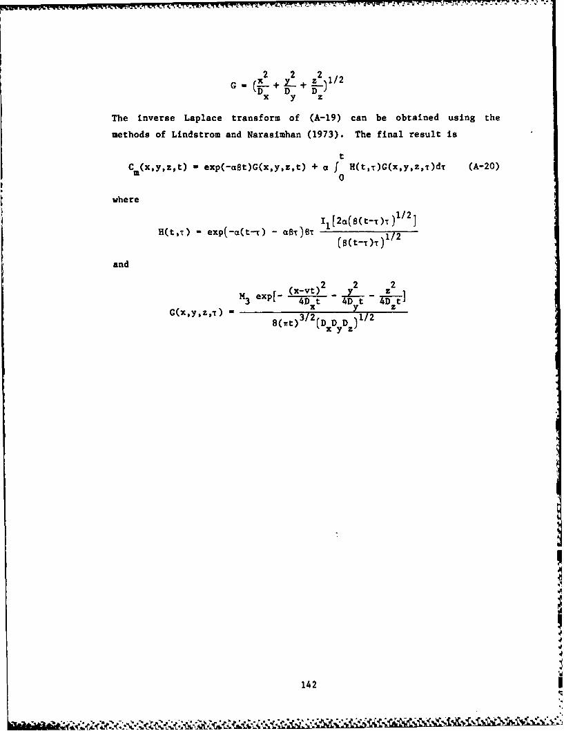
2 2 2G - + z 3_+ 1/ 2
x y z
The inverse Laplace transform of (A-19) can be obtained using the
methods of Lindstrom and Narasimhan (1973). The final result is
tC M(xy,z,t) - exp(-aBt)G(x,yz,t) + a f H(t,T)G(x,y,z,T)dT (A-20)mo
where
1/2
H(t,r) - exp(-c%(t--r) - 1B/2O(B(t-r)T)
1/ 2
and
S exp[- (x-vt)2 y2 _ Z23 4D t 0 t 0 t
G(xy2z,) - 1/28(,rt) (Dx D yD 1/2
142
, :-L ,a,-., . ,,.,-..' ,--,'-,-.,:.."- -,- ,","-:" - ,r "' . .e.-..'; : ' ;, .-,' ' ', ,',, ' 'K''W'e~w, , ,',:*er ¢'\' ' ' -/ . ' :

APPENDIX B
DERIVATION OF THE SOLUTION TO THE DIFFUSION MODEL
WITH SPHERICAL IMMOBILE ZONES
Differential Equations
3C m(xYZt) a2C a2C a2Cm 3C aCim-WD T- D m -D- - a (B-1)
at = x 2 y ay2 z az-2- x at
_ Ca _ - a (r a) (B-2)t 2 ar ar
fb
C 3(xyzt) 3 f r2C (r,x,y,zt)dr (B-3)im 0 a
Initial/Boundary Conditions
Cm(X,y,z,O) M3 6(x)6(y)6(z) (B-4a)
Cm(*0oy~z,=t) C(x*zt) C(xy, t) 0 (B-4b)
Ca(r,x,yzO) n Cim(X,y.zO) - 0 (B-4c)
Ca(Ox,ytztt) * (B-4d)
Ca(bx,ylz,t) n Cm(xyzt) (B-4e)
Following the methods of van Genuchten et al., (1984), take the
Laplace transform of (B-2), applying initial condition (B-4c) to obtain
the following ordinary differential equation:
d2Ca(rxyzs) 2 dCa 6 -(a+ i--r - - o (B-5)
dr2 rdr De a
Transforming boundary conditions (B-4d) and (B-4e) gives
z-(O,x*y~z,s) (B-6a)a
a (bxyz,-) = (x,y,z,s) (B-6b)
143

Solve the above ordinary differential equation with boundary conditions
to find
CM(x, y,zts)Ca(r,x,y,z,s) - 10 (b) io(0r) (B-7)
where
WI
Now take the Laplace transform of (B-3)
3 fb r2 a(rxy,zs)dr (B-8)
and substitute (B-7) into (B-8) to obtain
3C(xY , yz,s)i1 (wb)
:imxyzs) - wbi0 (wb) (B-9)
Take the Laplace transform of (B-i), using (B-9) and initial conditions
(B-4a) and (B-4c) to get the following differential equation
2.- 2- 2- a 3iba C- a C " a2Cm acm 38Si 1 (wb)
D D 2 D ax [) ] Tx ax2 Y ay zaz2
M - M36(x)6(y)6(z) (B-10)
Transforming boundary condition (B-4b) gives
(*-,y,,s) - C(x,~,~azs) - W(x,y,*.,s) - 0 (B-11)
A solution to (B-10) and (B-i) may be found using Fourier transforms.
As in Appendix A, the Fourier transformed solution is
H3
2(p,q,u,s) D 2 3 2 2 (B-12)Dp2 + Dq + Du + vip +Nx + y z
where
2 39i1(wb)N + S
wbo(wb)+
144

Note the similarity between Eq. B-12 and Eq. A-9. To obtain Cm(Xyz,s),
the methods of inverting the Fourier transform in the x-, y-, and z-
directions used in Appendix A are directly applicable. The result is
F
Cm(x,y,z,s) exp [-GO(s)] (B-13)
where
M3 exp(vx/2Dx)F = 3112
41r(DxDyDz)
2 2 ) /2G(x + L- + L-1/
x y z
22 2 1/2
Q(s) 4 + N2)x
To obtain the inverse Laplace transform of (B-13), the methods used by
Rasmuson and Neretnieks (1980), and van Genuchten et al. (1984) may be
followed directly. The final result, for the response to an instantane-
ous point source, is
Cm(x,y,z,t) ,
M3D e exp(vx/2Dx 2D e2t
b2 2(D DDz)1/2Gf 0 exp(-GZp Cos b2 - GZm) d' (B-14)
where
2 2 2
x y z
___1_ 12_ f 1 1 /,2 r SI2 +12)1/2pz - 2 p 1 2
3DB 2D A2 3D8
R1 4D -~) b 2 1 2 _+2 - 2
X = (Sinh 2A + Sin 2X) - 1 -2 (Sinh 2X - Sin 2X)1 Cosh 2X - Cos 2A '2 Cosh 2X - Cos 2X
145

-r -799W
APPENDIX C
DERIVATION OF ABSOLUTE SPATIAL MOMENTS
FOR THREE SOLUTE TRANSPORT MODELS
Local Equilibrium Model
ac .D a2 C+D a2 C+D a2 C vac(C1at x~ __T Dy~+DA- -- I (C-i)
ax ay az
C(x,yz,O) - M3 6(x)6(y)6(z) (C-2)
C(*oo,y,z,t) - C(x,*-,z~t) - C(xpyp*,Ot) - 0 (C-3)
Taking the Fourier transform of the equation and initial condition,
where p, q, u are the Fourier transform variables in the x-, y-,
z-directions, respectively, yields:
at(p,q,u,t) -D 1i2 P2 e( pq,u,t) + D 1i2q 2t(p,q,u,t)at xy
+ Dzi2u2C(p~q~u~t) - vip8(p,q,ut) (C-4a)
a(p~q,u,O) -M 3 (C-4b)
Solving for Z(p,qu,t) is straightforward:
C(p,q,u,t) - M3 e ~ -( 2DIq+Z u+i (C-5)
Applying the expression
2 lim -- -. dtpgut)}(C-6)Jkl p+0 dpi dq k du I
q+Ou+O
requires the differentiation of 8 (p,q,u,t) with respect to p, q, and u.
This operation is easily done. Taking the limit as the transform vari-
ables approach 0, gives:
146
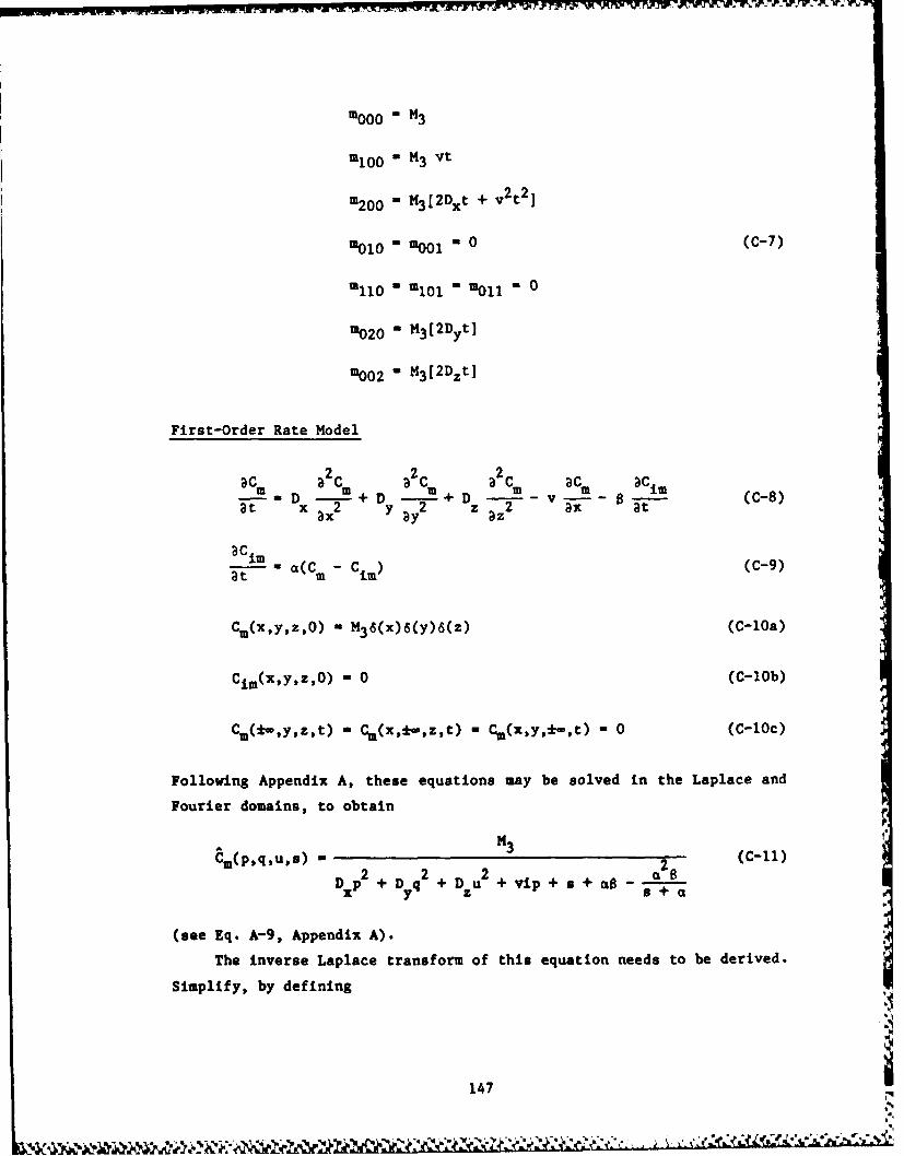
moo0 - M3
mo 0 = M3 Vt
m200 - M3 [2Dxt + v2t2]
-oO = om " 0 (C-7)
mll0 a 12101 = Moil M 0
M020 - M3 [2Dyt]
m0 0 2 - M3 [2Dzt]
First-Order Rate Model
ac c2C aC aCm aCimD -m+D -+ D -- v--B)
at x 2 yB 2 z 2 ax at
aCim
- a(C - Cim) (C-9)
Cm(x,y,z,O) = M36(x)S(y)6(z) (C-10a)
Cim(x,y,z,O) = 0 (C-lOb)
Cm(*in,y,z,t) CM(x,'*o,z,t) Cm(x*y,*-,t) = 0 (C-lOc)
Following Appendix A, these equations may be solved in the Laplace and
Fourier domains, to obtain
M3C3 (p,qu,s) 2 (C-11)
Dxp2 + Dyq2 + Dzu 2 + vip + s + a$
(see Eq. A-9, Appendix A).
The inverse Laplace transform of this equation needs to be derived.
Simplify, by defining
147

A - DXp 2 + D yq2 + D U2 + vip - i+ ci8
so
A M 3Cmp~~js I2 (C-12)
Multiply the numerator and denominator of the right-hand side of Eq.
4 C-12 byea + ai, to obtain
H 3(s + az)Cm(p,q~u,s) -2 2 (C-13)
(s + 0) + A(s + a) -ca
Defining E and F as the roots of the quadratic equation in the denomina-
tor of the right-hand side of Eq. C-13 gives:
H 3(s + ai)Cm~ptqtupsJ [(s + ai) - EJ[(s + ai) - F]
Use the following properties of Laplace transforms
L [Fs+ ai)] -et f(t)
and
FFt EEt
* (s - E)(s - F)~ F -E
to find
FFt EEt*Cm(pgqpupt) m ~ e [ - E C (C-14)
where E and F are functions of A, ai, and ~
* Differentiation of Eq. C-14 is straightforward, though tedious.
* Apply Eq. C-6, to find:
148

1 + 8 ct18
Mlo M3vt 2 [l + 82 e-at(l+8)] + 2M 3 vs [ -eit(1+S)j(+ 8) C(1 + 8)~ 1-e
M20' 2m 3D xt [l+ 02 -ct(l+0) + [1 eDt(+8
(+ B) [i 2c(1 + B) f-
+v 2t2 M3 + 3ea(61 6v 2 (B - 1)m 1 -e43'+G + 0)~ +~~8 ]+ 218)5 t~~~+)
+ I.6v2 t I4 3 ( 1Ot~l8 ) (C-15)
Moo- 3001 -0
M0120i (1+8)t2 2 e -at(l+S) ~+ 4M 3D y8 (G +0) (1 + B) [-
(1 3 8) [t + 82 e £t(l+)i + 4M 3D Z i 8 ~tlS+ 0) (1 + )
Diffusion Models
ac m 2CM V~ aDc IC aci- D -+D _ ---- 0 r (C-16)at x 2 y 2 ax2atax a~y a
ac a D e ac aat rv arrVDr(C17
Ci ;+ f vC. dr (C- 18)
C,(x,y,z,0) - M36(x)6(Y)tS(z) (C- 19a)
Ca(rgxgygz,O) m C13(xy,z,O) - 0 (C-19b)
149

C.(*-,yIZt) = C(x,*-,z6t) - Cz(x,y,*-,t) - 0 (C-19c)
C(0,x,y,z,t) -(C-19d)
Ca(bxy,z,t) = C,(xy,z,t) (C-19e)
Following Appendix B, these equations may be solved in the Laplace
and Fourier domains, to obtain
H3C,(pq,u~s) - -(-0
Dxp2 +Dyq2 + D +vp+ 2 (C2)
where
142 -3S8i(bN b i1(wb) + s for the spherical diffusion model
2 b 1 2 (wb)
= b Il(wb) + s for the cylindrical diffusion modelwb 1 0(wb)
N2 . Ss Sinh wb + s for the layered diffusion modelwb Cosh Lb
To derive the inverse Laplace transform of Eq. C-20, it is neces-
sary to apply Bromwich's complex inversion formula:
A1 f a+i-D e t
C3(p,q,u,t) - 1 U i e 8m ds
Using the same technique as Rosen (1954), Rasmuson and Neretnieks (1980),
and van Genuchten et al. (1984), who derived similar inversions, it can
be shown that
C3(p,q,u,t) 1 lim f + f + st ds (C-21)2wi i3*c 0 -iu ic -ic -- s(-1
where A(s) - Dxp2 + D yq2 + DzU2 + vip + N2 .
Perform the above integration, basically following the methods of
Rasmuson and Neretnieks (1980) and van Genuchten et al. (1984), to find:
150
I[ .e e. : . ; .-.---------- S.* .. I . - - - -

Cm(pqut) -
2D A 2 t 2D A 2t-
13 P3 Cos b2 + 02 Sin 2bm0 0 5b
2 + 2b+ 27 e D1 + a2
where
3DeBn, - Dxp 2 + D
q 2 + DU2 + 7 3De
2D A 2 3D 02e •
n2 = vp + + 2 '2
and *1 and *2 are as defined in Chapter 2 for the different immobile
region geometries. As p, q, and u approach zero, S1 and S2 are as
defined in Appendix B (with v - 0).
Use Eq. C-6, to write
M000 limr Cm(p,q,u,t) yo +rnp+O £0 21q+0u+0
F 2D A2t 2D X2I e ________________
4M3De - 1 Cos eb2 + n 2 Sin e2
+ "b b 2 2 b dX (C-22)eL1Differentiating Eq. C-22 by applying Liebnitz' rule, and then applying
Eq. C-6, leads to the following expressions:
urn M{3v 3vt M3vB
E*0 E(1+8)2 2(1+0)2 a(1+8)3
S2D A 2t 2D X2t
4M 3 vD e fa X 1 2 )Cos 2 + 2fl1 Sin 2De- b1 b2
151

77 r-- -v r W ra 773 T 77--- 7-7'WT -7 12i-
F 2M3Dx M3Dxt 2M3Dx8
m200 = lim 2 + 2M 3
C+0 we(1+o) (1+8) a(1+6) 3
2D A2t 2D t"(2 2 e + 2 Sin e
8Mxe 3 D D 1 2 b 2 b 2
+ -2 f A -2 +Wb 1 +n2
2 22 22L2M3vt M3vt2 6M3 ~v2 6M3 v28++ + +2+ 3 2 3 2 M5 4a v 2
ircl+8) 2(1+0) a (1+0) wrea(1+8)
3M3v2 t 3M3v2
a(1+0)4 c(l+6)
4
8(nv 2 D - 3 X n )Cos 2De A2 t _- 3 2 ) Sin 2De)3A 12 1
3 e b2
+ 2 f L 2 2 2f )Sn b2 dwb b (-1 + Re L
where for spherical diffusion:15D 315D 2
e ea =- T-- 9 c -- 7 -4b 2bB8
for cylindrical diffusion:
8D 48D 2e e
b2 , c = 7b b 0
for layered diffusion:
3D 15D 2
e ea - b c - bb 2b48
010 = Moo = 0
silo m 101 Mo11 - 0
152

U, 00 " 2M3Dy 3Dyt 2H3Dy83"020 "M2+ 2+ 3
C+O WC(1+B) (1+0) a(1+8)
t2D Aj 2 2 t2 fl) 2D:A 2 t j8MDD 2 +_2n+ 2n Sin e
+ - w b 2 f d A
2M3 Dz M3Dzt + 2M3Dzam2 2
2l m + 3 +CO LC(I+8 ) 2 (1+0) 2 a(l+s) 3
-(22D A2 2D A2
8M3DzD 1 2 + 2 1 2 Sin b2
irb2 2 + 22 jJeJ2 L
g,,
153
ABC%&

APPENDIX D
DERIVATION OF ABSOLUTE SPATIAL MOMENTS OF THE
IMMOBILE REGION SOLUTE DISTRIBUTION
First-Order Rate Model
In Appendix A it was found
'dx~yz~ = a C(X,y,z,s) (D1
m1 a + aDm''
Take the Fourier transform of (D-1):
s+aCim(Psq'u's) s+-- Cm(p,q,u,s) (D-2)
In Appendix C it was found
M3(s + a)_C(Pq'u's) - [(s + a) - EJ[(s + a) - F] (D-3)
Combining (D-2) and (D-3):
M3aCim(pq'u's) - [(s + a) - E][(s + a) - F] (D-4)
Follow Appendix C to invert the Laplace transform, to obtain
Cim(p,q,u,t) a ea [F - EtF: E ] (D-s)
Finally, differentiate Eq. D-5 and apply Eq. 3-23 to derive the follow-
ing absolute moments:
M30[1 - e -t(l+B) ]
no00 =1 + 0-M3vtB[l - 0 •-a t (1+ S ) ] M3v ( - 1)[l - •-at( + 8)]
(1+8)'2 + 3 .(l + 0)2 a(l + 1)
nolo nool -0
154

Diffusion Models
Follow Appendix B, to find
-- [N2 -si
C m(x,y,z,s) - (x ,y,z,s) (D-6)
where
30s il(wb)Ni(wb) + s for the spherical diffusion model
N2 s I (wb)
N2 . 2 II(b) + s for the cylindrical diffusion modelwb 1 0(wb)
N2 . ba Sinh(wb) + s for the layered diffusion model
wb Cosh(wb)
Take the Fourier transform of (D-6):
q . [N-]
Cim(p qqups) as Cm(psqu,ss (D-7)
In Appendix B it was found
M3H3Cm(p'qus) m Dxp2+ 2 + D u2 + vtp + N2 (D-8)
Vy z
Combining (D-7) and (D-8) yields:
M (N2 - s)
Cim(p'q'us) - (Dxp 2 2 +DU 2 2 (D-9)Dyq z +vip+N
Defining:
A(s) - Dxp2 + Dyq2 + Dzu 2 + vip + N2
gives:
-p2 qM3[2(s)- -Dq - D u -v v ]p - s]3impaquss =P zas n(s) (D-10)
Follow Appendix C to obtain the inverse Laplace transform of Clm(p,q,u,s),
using Bromwich's complex inversion formula, to find:
155

M3 M3 At H3 A
Cjm(pq.ut) - 3<* - 2(1+0) - _(1+8)_
40+
2D X2t 2DAtM3A 2M3A n 2 b2 1 e2
__ +_ 3 b b~ Id2a(1+8) WO f L + 2
r 1 22[ 2D A2t 2D A2t
H3 4M3D e1 Cos + Sin
20(1+0) 2 + 2 S] D -c1 2
where A - Dxp 2 + Dyq2 + DzU2 + vip
v(v + 2)D v - 3 for spherical diffusiona = b 2 e where v - 2 for cylindrical diffusion
v - I for layered diffusion
and n1 and Q2 are defined in Appendix C. Differentiating and applying
Eq. 3-23 leads to:
2D 2t 2DeA2t
M3 4M3D S 1 Cos 2- + a 2 Sin b2n300-lim 2(1+0) 3 e2 f 2 + 02b d
+0 b 2 :1 2
nlO 0 F lm .M3vt + M3vB + 3 vo(8-1)n100 2(1(0+ 2 2a(l+B 3
2D A 2t 2D A2te e
2vM - 02 Cos b 2 A1 Sin b2 (D-12)
f! X~n 2 dA
D 1 22De 2 2 2D A2t 2D t 2t
,,3.e f ( n 2 ) Co. b + 2nIf2 Sin b 2- -b f 2 2 2 I d+ '
no1 o - nool 0
156

APPENDIX E
BREAKTHROUGH RESPONSE DATA
157

1.9-
0.9 - Bromide
0.8- + Carbon Tetrachloridez0 * Bromoform
0.7 -a Tetra ch loroethylene
I-zW 0.6zo 0.5-C-)
0 .4Li
S 0.30z
0.2
0.1
0 100 200 300 400
TIME (days)
Figure E-1. Breakthrough response at well location x - 2.50 m,y =0.00 m, and z =-3.20 m.
1-
0.9- Bromide
0.8 -+ Carbon Tetrachloridez0 o Bromoform
0.7 -A Tetrachioroethylene
zW 0.6z0 0.5
0.0
0
N 0.4
S 0.3
0
0 100 200 300 400
TIME (days)
Figure E.2. Breakthrough response at well location x - 2.50 m,y - 1.25 m, and z - -3.62 m.
158

7tr "11-z ! Wr
0.9
0.8- - Bromide
+ Carbon Tetrachloride
z 0.7 -> Bromoform
0 A Tetra chiloroethyleneg 0.6I-zLiU 0.5-z0Ua 0.4LiN
< 0.3
0z 0.2
0.1
0
0 100 200 300 400
TIME (days)
Figure E.3. Breakthrough response at well location x f 5.00 m,y - 0.00 m, and z - -3.26 m.
0.1
0.09 -
0.08z0
0.07I-
zw 0.06Uzo 0.05
LiN 0.04
" O<W2 0.030z
0.02
0.01
0- I I I I
0 0.2 0.4 0.6 0.8Thousonds)ME (days)
Figure E.4. Tetrachloroethylene breakthrough response at welllocation x - 10.00 m, y - 4.60 m, and z - -3.88 m.
159
r "-". rt " "' -'.. "t"f., ., , ,, ¢ ' .,. ,. ; ,. ,. , .. . ; .r, :.,r ... ... .... ..... .....4'., .,r ,.,-. ,:-,% .. : % , . , . .o., , . .,-.,',, .,., , . €, , f ,t .ft - ,,

0.016
0.015
0.014
0.013z0 0.012* 0.011
z 0.01Li0 0.009zo 0.008C)
o 0.007 -LiJ
0.006
0.0050 0.004z
0.003
0.002
0.001 -00- I I I
0 0.2 0.4 0.6 0.8T housands)IME (days)
Figure E.5. Tetrachloroethylene breakthrough response at welllocation x 1 10.00 m, y = 4.60 m, and,;: - -4.48 m.
0.04
0.035
zo 0.03
z 0.025Li0zo 0.02
aLij
N 0.015.J
o 0.01z
0.005
0 I I
0 0.2 0.4 0.6 0.8housands)ME (days)
Figure E.6. Tetrachloroethylene breakthrough response at welllocation x - 13.10 m, y - 4.05 m, and z - -3.42 m.
160

0.06
0.05
z0o_
0.04
zhiUz
0 0.03-
0
z
0.01 -
0I0 0.2 0.4 0.6 0.8
rThou sands)IME (Cays)
Figure E.7. Tetrachloroethylene breakthrough response at welllocation x = 13.10 m, y 4.05 m, and z - -3.72 m.
0.19
0.18 + Carbon Tetrachloride
0.17 - Bromoform
0.16
0.15Z0 0.14
4 0.13w- 0.12z
LJ 0.11
Z 0.10Lo 0.09
L 0.08N.. 0.07
: 0.06
0 0.05Z 0.04-
0.03
0.02
0.01
0 0.2 0.4 0.6 0.8rhou sands)ME (days)
Figure E.8. Breakthrough response at vell location x - 18.00 m,y - 9.00 m, and z - -4.13 a.
161
,]

0.45-
z 0.4-- Bromide0 + Carbon Tetrachloride
i~0.35-0 Bromoform
zwA 0.3-Uzo' 0.25-
N .
U 0.5-
0.15
0.05-
0-NO0 0.2 0.4 0.6 0.8
housands)IM (days)
Figure E.9. Breakthrough response at well location x - 18.00 M,ky -9.00 m, and z -4.73 m.
0.7
0.6- Bromide
0 + Carbon TetrachlorideR 0.5-
4 0 Bromoform
zU 0.4-
z0U
W 0.3-N
fr 0.2 -0z
0.1
0 -NO
0 0.2 0.4 0.6 0.8
*Figure E.10. Breakthrough response at well location x - 21.00 m,£ y a 9.00 m, and z - -4.17 m.
162

-. ~~~771 n TI 7.~. ~ . .
0.4-
0.35-- Bromide
+ Carbon Tetrachloridez0 0.3- * Bromoformn
z 0.25-
zo 0.2
N 0.15-
o 0.1z
*0.05-
0 0.20.0.0.housands)
IM das
A Figure E.11. Breakthrough response at veil location x -21.00 mn,y 9.00 mn, and z --4.77 mn.
0.45-
0.4-
z 0.35-2ti
r~0.3-zU 0.25-z0L)a 0.2-wAN
4.i< 0.15-
0z 0.1
* 0.05
0 -- - -0 0.2 0.4 0.6 0.8
(Trhousands)TIME (days)
Figure E.12. Bromide breakthrough response at veil location x-24.00 an, y - 9.00 in, and z - -4.76 mn.
163

APPENDIX F
HYSTERESIS EXPERIMENT METHODOLOGY
A bottle-point partitioning technique to measure long-term sorption
(Ball and Roberts, 1985) was combined with a technique to measure long-
term desorption, in order to assess whether sorption/desorption of
tetrachloroethylene onto Borden aquifer material was hysteretic.
Sorption Experiments
Sorption experiments were conducted using the bottle-point parti-
tioning technique of Ball and Roberts (1985) to measure long-term sorp-tion while carefully controlling losses. Using this technique, a knownmass of groundwater synthesized to approximate aquifer conditions
(Wrtis et al., 1986) and a known mass of sorbent, consisting of homoge-
nized Borden aquifer material, were added to glass ampules and the
sorbent allowed to come to complete water saturation. A known amount of
carbon-14 labeled solute was then injected into the glass ampule, and
the ampule immediately flame-sealed. After sealing, the sample was
allowed to equilibrate over a 30-day period. After the 30 days, half
the samples were centrifuged (2000 rpm for 30 min), cracked open, and
supernatant immediately transferred to scintillation cocktail for count-
ing on a Packard Tricarb Model 4530 Scintillation Counter. This count
provided an accurate measure of the solute concentration in the aqueous
phase. By difference, the sorbed-phase concentration was determined,
thus determining a point on the sorption isotherm. Losses due to parti-
tioning to the glass ampule and to the small volume of air in the ampule
were accurately and reproducibly quantified using blanks without soil.
Desorption Experiments
Desorption experiments were then conducted upon those samples not
opened in the sorption experiments. These samples were placed into
specially fabricated stainless steel vessels. To minimize losses, the
vessels were constructed to be airtight and to have only stainless steel
in contact with the sample. Synthetic groundwater, which had been pre-
equilibrated with the aquifer material, was added to the vessel, the cap
to the vessel closed, and the vessel shaken vigorously and centrifuged
164

for 30 min. The shaking and centrifugation broke the glass ampule inthe steel vessel, causing the aquifer material and solute within theampule to be diluted by the synthetic groundwater in the vessel. Thesample was then allowed to equilibrate for 30 days. After the 30 days,
4 the steel vessel was centrifuged, opened, and the supernatant trans-ferred to scintillation cocktail for counting. As in the sorption
experiment, aqueous-phase concentration was thus directly measured, andthe sorbed-phase concentration determined by difference. Blanks showed
4 that losses over the course of the 60-day sorption/desorption experiment
amounted to less than 15%.
165

REFERENCES
Aris, R., 1958. On the dispersion of linear kinematic waves, Proc. R.Soc. London, Ser. A, 245, 268-277.
Baker, L. E., 1977. Effects of dispersion and dead-end pore volume inmiscible flooding, Soc. Pet. Eng. J., 17, 219-227.
Ball, W.P., 1986. Unpublished data.
Ball, W. P., and P. V. Roberts, 1985. Rate limited sorption of haloge-nated aliphatics onto sandy aquifer material--experimental resultsand implications for solute transport, EOS, 66(46), 894.
Bear, J., 1972. Dynamics of Fluids in Porous Media, American ElsevierPublishing Co., Inc., New York.
Bear, J., 1979. Hydraulics of Groundwater, McGraw-Hill, Inc., New York.
Bibby, R., 1979. A Numerical Model of Contamination by Mine DrainageWater of the Chalk Aquifer, Tilmanstone, Kent, Water ResearchCentre Report LR 1005, Medmenham Laboratory, Medmenham, Marlow,Bucks., Great Britain.
Bouwer, E. J., and P. L. McCarty, 1984. Modeling of trace organics bio-transformation in the subsurface, Ground Water, 22(4), 433-440.
Bracewell, R. N., 1978. The Fourier Transform and Its Applications, 2nded., McGraw-Hill Book Company, New York, pp. 141, 251.
Bremermann, H., 1963. Distributions, Complex Variables and Fourier
Transforms, Addison-Wesley, Inc., Reading, MA, p. 143.
Carnahan, C. L., and J. S. Remer, 1984. Nonequilibrium and equilibrium
sorption with a linear sorption isotherm during mass transportthrough an infinite porous medium: some analytical solutions,Journal of Hydrology, 73, 227-258.
Carslaw, H. S., and &. C. Jaeger, 1959. Conduction of Heat in Solids,Oxford University Press.
Chiou, C. T., L. J. Peters, and V. H. Freed, 1979. A physical conceptof soil-water equilibria for nonionic organic compounds, Science,206, 831-832.
Christodoulou, G. C., 1986. Dispersion respoise of two-layer flows,J. Env. Eng. Div., ASCE, 112(2), 433-438.
Coats, K. H., and B. D. Smith, 1964. Dead-end pore volume and disper-sion in porous media, Soc. Pet. Eng. J., 4, 73-84.
Crank, J., 1975. The Mathematics of Diffusion, 2nd ed., Oxford Univer-sity Press, Oxford.
166

Crittenden, J. C., N. J. Hutzler, D. G. Geyer, J. L. Oravitz, and G.Friedman, 1986. Transport of organic compounds with saturatedgroundwater flow: model development and parameter sensitivity,Water Resources Research, 22(3), 271-284.
Curtis, G. P., P. V. Roberts, and M. Reinhard, 1986. A natural gradientexperiment on solute transport in a sand aquifer. IV. Sorption oforganic solutes and its influence on mobility. Accepted for publi-cation, Water Resources Research.
Cussler, E. L., 1984. Diffusion Mass Transfer in Fluid Systems, Cam-bridge University Press, Cambridge.
Dance, J. T., 1980. Evaluation of reactive solute transport in ashallow unconfined sandy aquifer, M.S. Thesis, University of Water-loo, Waterloo, Ontario, 93pp.
Deisler, P. F., Jr., and R. H. Wilhelm, 1953. Diffusion in beds ofporous solids: measurement by frequency response techniques,Industrial and Engineering Chemistry Journal, 45, 1219.
Demond, A. H., 1984. Unpublished data.
De Smedt, F., and P. J. Wierenga, 1979a. Mass transfer in porous mediawith immobile water, Journal of Hydrology, 41, 59-67.
De Smedt, F., and P. J. Wierenga, 1979b. A generalized solution forsolute flow in soils with mobile and immobile water, Water Re-sources Research, 15(5), 1137-1141.
De Snedt, F., and P. J. Wierenga, 1984. Solute transfer through columns
of glass beads, Water Resources Research, 20(2), 225-232.
DiToro, D. M., 1985. A particle interaction model of reversible organicchemical sorption, Chemosphere, 14(10), 1503-1538.
Durant, M. G., 1986. Sorption of halogenated organic solutes in theBorden aquifer: evidence of spatial variability, Engineer Thesis,Dept. of Civil Engineering, Stanford University, Stanford, CA.
Freyberg, D. L., 1985. Personal communication.
Freyberg, D. L., 1986. A natural gradient experiment on solute trans-port in a sand aquifer: II. Spatial moments and the advection anddispersion of nonreactive tracers. Accepted for publication, WaterResources Research.
Gelhar, L. W., and C. L. Axness, 1983. Three-dimensional stochasticanalysis of macrodispersion in aquifers, Water Resources Research,19(1), 161-180.
Gelhar, L. W., A. L. Gutjahr, and R. L. Naff, 1979. Stochastic analysisof macrodispersion in a stratified aquifer, Water Resources Re-search, 15(6), 1387-1397.
167
' " ' " " .. . . ' "' " iI . ~ . . . .--- ' U .* *. - P . . . . .

Gillham, R. W., E. A. Sudicky, J. A. Cherry, and E. 0. Frind, 1984. Anadvection-diffusion concept for solute transport in heterogeneousunconsolidated geological deposits, Water Resources Research,20(3), 369-378.
Goltz, M. N., and P. V. Roberts, 1984. Mass transfer effects on ground-water transport of organic solutes. Presented at ASCE Annual Con-vention, San Francisco, 1-5 October, 1984.
Goltz, M. N., and P. V. Roberts, 1986. Interpreting organic solutetransport data from a field experiment using physical nonequilib-rium models, Journal of Contaminant Hydrology, 1, 77-93.
Gradshteyn, I. S., and I. M. Ryzhik, 1980. Table of Integrals, Series,and Products, Academic Press, New York.
Gschwend, P. M., and S. C. Wu, 1985. On the constancy of sediment-waterpartition coefficients of hydrophobic organic pollutants, Environ.Sci. Technol., 19(1), 90-96.
GUven, 0., F. J. Molz, and J. G. Melville, 1984. An analysis of disper-sion in a stratified aquifer, Water Resources Research, 20(10),1337-1354.
Hornsby, A. G., and J. M. Davidson, 1973. Solution and adsorbed fluo-meturon concentration distribution in a water-saturated soil: ex-perimental and predicted evaluation, Soil Sci. Soc. Am. Proc., 37,823-828.
Horzempa, L. M., and D. M. DiToro, 1983. The extent of reversibility ofpolychlorinated biphenyl adsorption, Water Research, 17(8),851-859.
Hunt, B., 1978. Dispersive sources in uniform groundwater flow,J. Hydraulics Div., ASCE, 104(HYl), 75-85.
Hutzler, N. J., J. C. Crittenden, J. S. Gierke, and A. S. Johnson, 1986.Transport of organic compounds with saturated groundwater flow:experimental results, Water Resources Research, 22(3), 285-295.
IMSL Library Reference Manual, 1982. The IM9L Library, 9th ed., IMSL,Houston, TX.
Karickhoff, S. W., 1984. Organic pollutant sorption in aquatic systems,J. Hydraulics Div., ASCE, 110(6), 707-735.
Koch, D. L., and J. F. Brady, 1986. Nonlocal dispersion in porousmedia: nonmechanical effects. Submitted to Chem. Eng. Sci.
Kucera, E., 1965. Contribution to the theory of chromatography. Linearnon-equilibrium elution chromatography, J. Chromatog., 19, 237-248.
Leland, D. F., and D. Hillel, 1982. A field study of solute dispersionin a shallow, unconfined aquifer, Soil Sci. Soc. Am. J., 46,905-912.
168

Lindstrom, F. T., and M. N. L. Narasimhan, 1973. Mathematical theory ofa kinetic model for dispersion of previously distributed chemicalsin a sorbing porous medium, SIAM J. Appl. Math., 24, 496-510.
MacFarlane, D. S., J. A. Cherry, R. W. Gillham, and E. A. Sudicky, 1983.Migration of contaminants in groundwater at a landfill: a casestudy, Journal of Hydrology, 63, 1-29.
Mackay, D. M., D. L. Freyberg, P. V. Roberts, and J. A. Cherry, 1986. Anatural gradient experiment on solute transport in a sand aquifer:I. Approach and overview of plume movement. Accepted for publica-tion, Water Resources Research.
Matheron, G., and G. de Marsily, 1980. Is transport in porous mediaalways diffusive? A counterexample, Water Resources Research, 16(5),901-917.
Mercado, A., 1967. The spreading pattern of injected water in a perme-able stratified aquifer, Symposium of Haifa, Artificial Rechargeand Management of Aquifers, Publ. 72, pp. 23-36, Int. Assoc.Hydrol. Sci., Gentbrugge, Belgium.
Miller, C. T., and W. J. Weber, Jr., 1986. Sorption of hydrophobic or-ganic pollutants in saturated soil systems, Journal of ContaminantHydrology, 1(1/2), 243-261.
Nkedi-Kizza, P., P. S. C. Rao, R. E. Jessup, and J. M. Davidson, 1982.Ion exchange and diffusive mass transfer during miscible displace-ment through an aggregated oxisol, Soil Sci. Soc. Am. J., 46,471-476.
Nkedi-Kizza, P., J. W. Biggar, H. M. Selim, M. Th. van Genuchten, P. J.Wierenga, J. M. Davidson, and D. R. Nielsen, 1984. On the equiva-lence of two conceptual models for describing ion exchange duringtransport through an aggregated oxisol, Water Resources Research,20(8), 1123-1130.
National Research Council (NRC), 1984. Groundwater Contamination, Panelon Groundwater Contamination, National Research Council, NationalAcademy Press, Washington, D.C., 17 9pp.
O'Hannesin, S. F., 1981. Spatial variability of grain-size parametersand hydraulic conductivity at a dispersion test site, Bachelor ofEnvironmental Studies Honours Report, University of Waterloo,Waterloo, Ontario, 46pp.
Parker, J. C., and A. J. Valocchi, 1986. Constraints on the validity ofequilibrium and first-order kinetic transport models in structuredsoils, Water Resources Research, 22(3), 399-407.
Passioura, J. B., 1971. Hydrodynamic dispersion in aggregated media.1. Theory, Soil Science, 111(6), 339-344.
169

M 37"-
Pellett, G. L., 1966. Longitudinal dispersion, intraparticle diffusion,and liquid-phase mass transfer during flow through multiparticlesystems, Tappi, 49, 75-82.
Prasher, B. D., and Y. H. Ma, 1977. Liquid diffusion in microporousalumina pellets, AIChE J., 23(3), 303-311.
Rao, P. S. C., J. M. Davidson, R. E. Jessup, and H. M. Selim, 1979.Evaluation of conceptual models for describing nonequilibrium ad-sorption-desorption of pesticides during steady-flow in soils, SoilSci. Soc. Am. J., 43, 22-28.
Rao, P. S. C., D. E. Rolston, R. E. Jessup, and J. M. Davidson, 1980.Solute transport in aggregated porous media: theoretical andexperimental evaluation, Soil Sci. Soc. Am. J., 44, 1139-1146.
Rasmuson, A., and I. Neretnieks, 1980. Exact solution of a model fordiffusion in particles and longitudinal dispersion in packed beds,AIChE J., 26, 686-690.
Rasmuson, A., and I. Neretnieks, 1981. Migration of radionuclides infissured rock: The influence of micropore diffusion and longitudi-nal dispersion, J. Geophys. Res., 86(B5), 3749-3758.
Reynolds, W. D., R. W. Gillham, and J. A. Cherry, 1982. Evaluation of =
distribution coefficients for the prediction of strontium andcesium migration in a uniform sand, Can. Geotech. J., 19, 92-103.
Roberts, P. V., 1966. The adsorption of normal paraffins from binaryliquid solutions by molecular sieve 5A adsorbent, Ph.D. Thesis,Cornell University. University Microfilms, Inc., Ann Arbor, MI.
Roberts, P. V., J. Schreiner, and G. D. Hopkins, 1982. Field study oforganic water quality changes during groundwater recharge in thePalo Alto Baylands, Water Research, 16, 1025-1035.
Roberts, P. V., M. N. Goltz, and D. M. Mackay, 1986. A natural gradientexperiment on solute transport in a sand aquifer: III. Retardationestimates and mass balances for organic solutes. Accepted for pub-lication, Water Resources Research.
Rosen, J. B., 1954. General numerical solution for solid diffusion infixed-beds, Ind. Eng. Chem. Journal, 46, 1590.
Satterfield, C. N., C. K. Colton, and W. H. Pitcher, Jr., 1973.Restricted diffusion in liquids within fine pores, AIChE J., 19(3),628-635.
Schneider, P., and J. M. Smith, 1968. Adsorption rate constants fromchromatography, AIChE J., 14(5), 762-771.
Schwartz, F. W., 1977. Macroscopic dispersion in porous media: thecontrolling factors, Water Resources Research, 13(4), 743-752.
170

Spiegel, M. R., 1968. Mathematical Handbook of Formulas and Tables,McGraw-Hill Book Company, Inc., New York.
Smith, L., and F. W. Schwartz, 1980. Mass transport. 1. A stochastic
analysis of macroscopic dispersion, Water Resources Research,16(2), 303-313.
Sudicky, E. A., 1983. An advection-diffusion theory of contaminant
transport for stratified porous media, Ph.D. Thesis, 203pp., Uni-versity of Waterloo, Waterloo, Ontario.
Sudicky, E. A., 1986. A natural gradient experiment on solute transport
in a sand aquifer: V. Spatial variability of hydraulic conductiv-ity. Accepted for publication, Water Resources Research.
Sudicky, E. A. and E. 0. Frind, 1982. Contaminant transport in frac-
tured porous media: Analytical solutions for a system of parallelfractures, Water Resources Research, 18(6), 1634-1642.
Sudicky, E. A., J. A. Cherry, and E. 0. Frind, 1983. Migration of
contaminants in groundwater at a landfill: a case study. 4. Anatural-gradient dispersion test, Journal of Hydrology, 63, 81-108.
Swanson, R. A., and G. R. Dutt, 1973. Chemical and physical processes
that affect atrazine movement and distribution in soil systems,Soil Sci. Soc. Am. Proc., 37, 872-876.
U.S. Environmental Protection Agency (EPA), 1980. Groundwater Protec-
tion, Washington, D.C., 36pp.
Valocchi, A. J., 1985a. Validity of the local equilibrium assumptionfor modeling sorbing solute transport through homogeneous soils,
Water Resources Research, 21(6), 808-820.
Valocchi, A. J., 1985b. Personal communication.
van Genuchten, M. Th., 1985. A general approach for modeling solute
transport in structured soils. In Hydrogeology of Rocks of LowPermeability, Proc. 17th Int. Congress, Int. Assoc. of Hydrogeolo-gists, Tucson, AZ, January 1985, pp. 513-526.
van Genuchten, M. Th., and P. J. Wierenga, 1976. Mass transfer studiesin sorbing porous media: I. Analytical Solutions, Soil Sci. Soc.Am. J., 40, 473-480.
van Genuchten, M. Th., and P. J. Wierenga, 1977. Mass transfer studies13 sorbing porous media: II. Experimental evaluation with tritium( H20), Soil Sci. Soc. Am. J., 41, 272-278.
van Genuchten, M. Th., and R. W. Cleary, 1982. Movement of solute insoil: computer-simulated and laboratory results. In SoilChemistry. B. Physico-Chemical Models, G. H. Bolt (Ed.), ElsevierScientific Publishing Co., pp. 349-386.
171
.-o
t '~:. .** ~ *, S~~~ ~ ~ . - ' '.5. . '

van Genuchten, M. Th., J. M. Davidson, and P. J. Wierenga, 1974. Anevaluation of kinetic and equilibrium equations for the predictionof pesticide movement through porous media, Soil Sci. Soc. Am.Proc., 38, 29-35.
van Genuchten, M. Th., P. J. Wierenga, and G. A. O'Connor, 1977. Masstransfer studies in sorbing porous media: III. Experimental evalu-ation with 2,4,5-T, Soil Sci. Soc. Am. J., 41, 278-285.
van Genuchten, M. Th., D. H. Tang, and R. Guennelon, 1984. Some exactsolutions for solute transport through soils containing large cy-lindrical macropores, Water Resources Research, 20(3), 335-346.
Vermuelen, T., 1953. Theory for irreversible and constant pattern solid
diffusion, Ind. Eng. Chem. Journal, 45, 1664.
Wakao, N., and S. Kaguei, 1982. Heat and Mass Transfer in Packed Beds,Gordon and Breach Science Publishers, New York.
Wakao, N., and J. M. Smith, 1962. Diffusion in catalyst pellets, Chem.
Eng. Sci., 17, 825-834.
Warren, J. E., and F, F. Skiba, 1964. Macroscopic dispersion, Soc. Pet.Eng. J., 4, 215-230.
Wilke, C. R., and P. Chang, 1955. Correlation of diffusion coefficientsin dilute solutions, AIChE J., 1(2), 264-270.
Wilson, E. J., and C. J. Geankopolis, 1966. Liquid mass transfer atvery low Reynolds numbers in packed beds, Ind. Eng. Chem. Funda-mentals, 5(1), 9-14.
Wood, A. L., and J. M. Davidson, 1975. Fluometuron and water contentdistributions during infiltration: measured and calculated, SoilSci. Soc. Am. Proc., 39, 820-825.
172

II
j
a
ad
.4
-a... '*.:-~ ~ - ~ .*. a. *. *.s*..~.-. * * - a * **ar~ - a ~ -


![Analytical Methods Diffusion NMR Spectroscopy in ... · Diffusion NMR Spectroscopy in Supramolecular and Combinatorial Chemistry: ... copy [22] laid the ... homogeneous system the](https://img.dokumen.tips/doc/110x75/5afef5407f8b9a444f8f87da/analytical-methods-diffusion-nmr-spectroscopy-in-nmr-spectroscopy-in-supramolecular.jpg)