Embed Size (px)
Citation preview

A SIMULATION HODEL OF THE COMBINED TRANSPORT
OF WATER AND HEAT PRODUCED BY A THERMAL
GRADIENT IN POROUS MEDIA
Th.J.M. Blom
S.R. Troelstra
REPORT no. 6 , 19 7 2
dept. of Theoretical Production Ecology
Agricultural University
WAGE~INGEN - THE NETHERLANDS
: ' I :_ . :·· I ·.
I,
, ... I'
I I -.-

List of Internal Reports of Department of Theoretical Production Ecology:
No: 1 D. Barel, F. van Egmond, C. de Jonge, M.J.Frissel, M. Leistra, C.T. de Wit.
1969. Simulatie van de diffusie in lineaire, cylindrische en sferische systemen.
Werkgroep: Simulatie van transport in grond en plant.
2 L. Evangelisti and R. van der Weert. 1971. A simulation model for transpiration of
crops.
3 J.R. Lambert and F.W.T. Penning de Vries. 1973. Dynamics of water in the soil-plant-atmosphere system: a model named TROIKA.
4 M. Tollenaar. 1971. De fotosynthetische capaciteit.
4a J.N.M. Stricker. 1971. Berekening van de wortellengte per cm3 grond.
5 L Stroosnijder en H. van Keulen. 1972. Waterbeweging naar de plantenwortel.
A SIMULATION HODEL OF THE COMBINED TRANSPORT
OF WATER AND HEAT PRODUCED BY A THERMAL
GRADIENT IN POROUS MEDIA
Th . J. M. B 1om
S. R. Troe ls tra
REPORT no. 6, 1972
dept. of Theoretical Production Ecology
Agricultural University
WAGE~INGEN - THE NETHERLANDS
I I I .~.
I (


Contents
l. Introduction
2. Theory
2. I. V.:1por transfer
2.2. Liquid trdnsfer
2.3. Total moisture transfer
2.4. Heat transfer
2.5. The equations describing combined moisture
and heat transfer
3. The simulation program
3. 1. The initial segment of the program
3.2. The dynamic segment of the program
Page
4
5
10
11
12
14
15
16
18
3. 2. 1. The calculation of the overall the rrna 1 conductivity 18
3. 2. 2. The calculation of s
3.2.3. The thermal and isothermal moisture diffusivities
3.2.4. Flow of moisture
3.2.5. Flow of heat
3.2.6. The output control
4. Results
4.1. Heat-moisture flmoJ in a soil column due to a sudden
increase (or decrease) of the temperature at one side
of the column for different initial moisture contents
4.1. l. Initial moisture content
4.1 .2. Temperature gradient
4.1 .3. Hydraulic conductivity and matric suction
4. 1.4. The calculation of :\(TCN), s(ZETA),' and the
thermal moisture diffusivi ties (DTV ,DTL) in
the rr:odel
4.1.5. Thermal conductivity
4. 1.6. Integration method ·
4.1. 7. The 'sim~lation of an experiment
4.2. Heat-moisture flow in a soil column due to a sinusoidal
temperature variation at one side of the column for
different initial moisture contents
5. Discussion
6. Summary
Appendix I . Definition of symbols
Appendix II· Symbolic names simulation model
Re fe renee s
22
23
26
28
30
37
37
38
39
39
40
41
42
42
43
46
48
49
52
54
l· I


I. Introduction
During the past twenty years much attention has been given to the
phenomenon of combined heat-moisture transfer in porous materials,
particularly in soils (e.g. Philip and De Vries, 1957; Cary, 1965; Rose,
1968a,b; Letey, 1968; Hadas, 1968; Cassel et al., 1969; Fritton et al.,
1970; and references cited by these authors). The fact that a temperature
gradient can.result in movement of soil water has been reported as early
as 1915 (Bouyoucos; cited by Rose, 1968a).
Soils under natural field conditions are subjected to continuous
temperature fluctuations and two significant changes of temperature in the
soil profile can be distinguished. The first one is caused by the daily
radiation cycle and results 1n a temperature wave which penetrates the
soil up to a depth of about 35 em, the most pronounced effects occurring
1n the upper 5-10 em. The annual or seasonal radiation cycle gives rise
to a second temperature wave penetrating the soil to a considerably greater
depth than the diurnal wave: of the order of 10 meters. The thermal
gradients brought about by these temperature waves tend to move soil
moisture in both the vapor and the liquid phase, while the direction of
movement changes every 12 hours and 6 months for the daily and seasonal
w~ves respectively.
Lebedeff (1927; cited by Rose, 1968a, and Cassel et al., 1969)
concluded from a field experiment in Russia that the temperature gradient
associated with the annual wave can cause an upward moisture movement
(vapor phase) of more than 6 em of soil water in a winter period. This
lS a considerable amount of water moving through the soil profile, which
most likely has to be partly related to freezing processes (density of
saturated water vapor over 1ce is less than over liquid water of the same
temperature).
Cary ( 1966) mentions four possible reasons why water flm~1s 1n the
liquid phase under the influence of a temperature gradient. A difference
in the density of water vapor due to a temperature difference will also
create a diffusive .flmv of \vater vapor. In general the flow of moisture
occurs from warmer to cooler areas and the proportion of water movement
as vapor to that as liquid will increase with decreasing soil water content.
An 1ncrease of the moisture content in the cold region may eventually
originate a flux in the opposite direction, i.e. from cold to hot, which
will be predominantly in the liquid phase.

- 2 -
Quite a few laboratory experiments on this subject .:.Hid related aspects
have been conducted since 1950 (e.g. references cited by Philip and De
Vries, 1957, and Rose, J968a). The quantitative implications of all this
research for soil moisture transport in the field environment, however,
have been inadequately investigated and different conclusions have been
drawn with respect to this matter (Rose, 1968a).
The importance of these combined processes of heat and moisture tr9ns
must be looked at especially with reference to evapotranspiration of soils
of the arid regions, temperature regulation of seed-beds, and such-like.
If thermal vapor movement is of any agricultural significance, it will be
under conditions of relatively low water contents (Rose, 1966). Results of
work done by Rose (1968a, b, c) indicate that under field conditions where
daytime radiation is high, and consequently high temperature gradients in
the soil profile, the net vapor transfer (principally a thennal flm..r) ls
of comparable magnitude to net moisture transfer in the liquid phase
(principally an isothennal flow) at suctions as lm..r as 200-300 mbars. At
suctions greater than about 5 bars vapor transfer was found to be the
dominant·mechanism of transport. According to Rose (J968b) vapor transport
may be inportant in special circumstances in the water economy of plants,
particularly in the germination and early establishment phases of plant
growth. Moreover, the thermally induced moisture flow may significantly
affect the net transfer of salts and plant nutrients (Cary, 1966; Rose,
1968b), either directly (thermal liquid flow) or indirectly by changing
moisture content gradients (returning capillary flow).
The purpose of this report is to present a simulation model for the
combined flow of moisture and heat through porous media such as soils,
\..rritten in CSMP (Continuous System Modeling Program). Since in the system
under consideration an imposed temperature difference will cause several
properties to change simultaneously with time (transient-state), an
analytical solution of the involved heat and moisture fluxes is very
complicated if not impossible. In that case simulation may provide a means
to solve the transient-state situation by assuming successively changing
steady-state systems·
The described model lS based upon an approach advanced by Philip
and De Vries (1957). Before Philip and De Vries (1957) had developed
their theory, som~ investigators used a modification of Fick's law of
diffusion in describing soil water movement due to temper~ture gradients.
In fact the Philip -De Vries theor~ is an extension of Fick 1 s modified law.

- 3 -
ln c.1ddition to the Philip -De Vries theory, Taylur :.1r1d Cary (Toylor
~nd C~ry, 1960 and 1964; Cary and Taylor, 1962a, b; Cary, 1965) have
proposed a theory based upon the thermodynamics of irreversible processes.
Their equations are of the same general form as those developed by Philip
arid De Vries and so far the application of irreversible thermodynamics
to the problem of interacting heat and moisture fluxes in soils did not
produce any new information (Rose, 1968b).
Recently, Cassel et al. (1969) applied both the Philip-De Vries
theory and the Taylor-Cary theory to their experimental results. Net water
fluxes predicted by the Philip-De Vries theory agreed reasonably well with
observed values (about equal), while application of the Taylor-Cary theory
led to seriously underestimated values (off by a factor 10-40). Results
obtained by Fritton et al. (1970) are also in favor of the Philip-De Vries
theory.
The facts mentioned before seem to justify the use of the Philip
De Vries theory as a basis for the simulation model. The presented model
must be viewed as a preliminary one, and will no doubt await further
·improvements and modifications. In order to apply to open systems, for
example, an evaporation term needs to be included. It has been a first
aim to simulate the combined transport processes·occurring in the relatively
simple case of a (for moisture) closed soil column of finite length.
I.

- 4 -
2. Theory
A definition of the symbols used 1n this section 1s g1ven separately
1n Appendix I.
Supposing the transport process 1n a porous medium to be a frictional
flm.,r with a frictional force proportional to the flo-.;;.,r rate, one may assume
that the flux (qA) in a certain di~ection lS proportional to the driving
force (F) in this direction. Thus
B. F-r (x)
( 1)
The potential of the agent related to the driving force F 1s given by
-+ \j;F-- f F(x) (2)
where the m1nus s1gn indicates that the potential increases if the direction
of the driving force is opposed to the positive x-direction. The potential
lS a scalar quantity, whereas the driving force and the flux are vectors.
The total potential of the agent is obtained by adding all its partial
potentials.
From (2) one may substitute -+
F (x) (=-grad \);F) 1n (1), \<Jhich gives
- B grad 0 ·F (3)
Denoting the amount of the agent A per unit of volume by A, Wp and the
differential capacity of the medium for the agent A(CA) are formally
combined by
(4)
Transformation of (3) and substitution of (4) yields
(5)
Defining the diffusivity D as the ratio of transport coefficient and
capacity (B/C), one obtains
- D grad A (6)

- 5 -
Applying the continuity condition (principle of the cons~rvation of
matter) leads to
oA/ot - grad qA(x) grad (D grad A) (7)
For steady-state situations qA(x) lS constant, and accordingly oA/ot 0.
The steady-state equation of vapor diffusion ln alr (Fick's law) lS
quite similar to (6) and may be written as
= - D grad p a
(Sa)
Instead of taking the water vapor density gradient one may also develop
different expressions by using the gradient of the partial pressure of -1
water vapor in units of either dyne em (e') or mrn Hg (e), which results
in (Rose, 196Sa)
= - (D /R T) grad e' a w
- 1.36 (D g/R T) grade a w (Sb)
Vapor diffusion in a porous material (e.g. soil) will be less than in alr,
because of a longer path length (resulting in a smaller gradient) and a
volumetric air content a< J. Further a mass-flow factor v(= P/(P-e)) may
be introduced to allow for the mass-flow of water vapor due to a gradient
of the total gas pressure. At normal soil temperatures, this factor is
clearly quite close to unity. Therefore, for vapor diffusion in soils (Sa)
be comes
q = - (D vaa) grad p v a (9)
As pointed out by Philip and De Vrie~ (1957), Pick's law of diffusion
modified to apply for vapor movement in porous media (eq. (9)), denoted
in their paper as the ~'simple theory", will underpredict ,,rater vapor
transport occurring under thermal gradients. They examined some literature
data and made quantitative comparisons, which generally yielded values
for the ratio of observed transfer .to the value predictid by the simple
theory of about 3-10. Cassel et al. (1969) calculated this rati_o from their

- 6 -
own experimental data and found values which are of tl1e s~me order of
magnitude: about 5.
For water vapor 1n the soil air 1n equilibrium with the water in the
medium one may write the following relationship, neglecting possible osmotic
in f 1 u en c e s ( s e e , for ex amp 1 e , B o 1 t e t a 1 . , I 9 6 5 , p . 2 6 )
(RT/18) ln (e/e ) s
(RT/18) ln (p/p ) R T ln h (10) 0 t,..7
-1 Expressing the water pressure 1n em H
20 instead of erg g , gives
(R T/g) ln h w
or
From (10) and (I 1) it follows that
p = p h 0
Differentiating equation (12), one finds
grad p h grad p + p grad h 0 0
( 1 1 )
( 12)
( 13)
p0
lS independent of the water content of the medium and (for reasons
discussed by Philip and De Vries, 1957) oh/oT may be taken as zero in the
full range of h. In other words, one may conclude that p0
is a function
of T only and h is a function of 8 only. Thus (13) may be re-written as
grad p = h (op /6T) grad T + p0
(oh/88) grad 8 . . o.
Taking the derivative of (1 1) with respect to 8
oh/oe
and substituting p for p h, equation (14) becomes 0
grad p h (op /oT) grad T + (gp/R T) (6~/oe) grad 0 0 . w
( 14)
( 1 5)
(16)

- 7 -
-l Inserting (16) into (9) and expressing the flux 1n em s~c yields
- (D vJ.a/p1
) !Lh (6p /6T) grad T + (gp/R T) C'.)~S) grad 0} (17) a o w
- DT grad T - DP grad 8 V vV
Equation (9) has now been separated into a thermally induced and an
isothermally induced vapor flux, as represented by the first and second.
term on the right-hand side of equation (17) respectively.
Writing S for 6p /6T and 1/C for 6~/68, the vapor diffusivities 0 w
are given by
DTv D vaahS/p1 a
(18)
and
Dev D vaagp/pl R TC a 'i.v w
(19)
So far, the equations refer to the simple theory of vapor diffusion
with the assumption that no interaction of the vapor phase \vith either
the liquid phase or the solid phase will take place.
At this point the further development of the theory as has been
suggested by Philip and De Vries (1957) may be introduced. Their extended
theory can be summarized as follows,
At (liquid) moisture content values 81
< 8K' ~here 8K is the value
of e1
at which K becomes practically zero (no liquid continuity and
consequently no significant moisture transfer ln the liquid phase),
moisture (vapor) transfer is_ not just restricted to the air-filled pore
space, but can also proceed through the isolated regions of liquid between
the soil particles, which are assumed to be paths of low resistance to
vapor (Rose, 1968a), by condensing and evaporating processes on the upstream
and do\mstrearn side respectively. In other words, regarding the flow as
a seri~s-parallel proces~, the entire porosity ET (= a+ e), and not just
the gas-filled part ~' is effective in vapor diffusion under such moisture
conditions. The value of eK will depend upon soil texture (Philip and
De Vries, 1957), being greater and occurring at relatively high suction
levels in finer-te~tured soils. Vapor transport becomes dominant at suctions
of 5 to 15 bars (Slatyer, 1967; Rose, 1968b). Kramer (1969) mentions a
suction of 15 bars as the point where the liquid continuity is broken.

- 8 -
A second modification arises from the fact that the thermal gradient
across air-filled pores, (grad T)a' which is effectiv~ in promoting vapor
diffusion, can considerably exceed the mean overall temperature gradient,
grad T, in the medium by a factors~ I. Note that one has about the same
temperature difference over a shorter distance when considering only the
air-filled pores (see for instance Figure 42 in Rose, 1966). Thus
(grad T) I grad T a
(20)
From (17) and (18) it follows that for a single air-filled pore (aa I)
the vapor flux due to a temperature gradient may be given by
- (D vhS/p1
) (grad T) a a
\.Jhere (grad T) represents the thermal gradient in the pore. a -
(21)
Re-defining (grad T) as the average temperature gradient ln all aira
filled pores, (21) is also applicable to the vapor flux in the air-filled
porosity. of the medium, simply by multiplying with the factor~
the tortuosity factor a being included in (grad T) . . a
(22)
Assuming the liquid flow through the isolated wedges of liquid to
equal the vapor flux through the air-filled pores, in accordance with
the suggestions mentioned before, the revised theory for the total vapor
flux density due to a temperature gradient lS expressed by (for Bl< 8K)
-{(a+ 8) Da vhS/p 1 } (grad T)a =- DTv grad T (23)
Using (20), the thermal vapor diffusivity as predicted by the revised
theory is thus
= (a + 8) D a (24)
In the following the symbol DTv will be used in this sense to distinguish
it from the value predicted by the simple theory (eq. (18)), unless otherwise
noted.
i i I.
- 9 -
Defining (grad T). as the temperature gradient av~raged over the l
fractional volume, X., occupied by the component i in the medium, the value of l
s can be calculated for a system made up of n constituents from (20) with
(Philip and De Vries, 1957)
grad T n L:
i=O X. (grad T).
l l (25)
The actual method of calculating s as indicated by De Vries (1963)
will be described under section 3. Generally the value of s will be ln the
range 1.0- 2.5 depending, among other things, on total porosity, volumetric
moisture content, and temperature (Philip and De Vries, 1957; Rose, 1968a).
As will be shov.rn in 4.1.4., a value of about 1.8 will usually be a good
approximation for s• If specific data as moisture content and total porosity
of the soil are available, a more accurate value may be estimated from
Table 5.
The picture changes when e1 > 8K' and the degree of liquid continuity
increases from zero (at e1 = 8K) on. Thus for moisture contents increasing
from this point the degree of vapor continuity decreases, whereas liquid
moisture transfer due to thermally induced capillary potential gradients
becomes gradually more important. The decrease of the vapor-induced
transfer through isolated liquid wedges mentioned before is not only due
to a reduction in the number of islands and in the opportunity for vapor
transfer (air-filled porosity decreases) but also to an increase in the
radii of curvature of the menisci to the point where automatic adjustment
to the vapor flux is no longer possible (Philip and De Vries, 1957). One
may suppose, therefore, that the effective cross-section for the serles-
parallel vapor transfer (interacting with the liquid phase) will decrease ~
as 81
increases from 8K; Assuming as a first approximation a linear decrease,
the term (a + 8) in equations (23) and (24) may be replaced by a term
{ a + f(a)8} with f(a) = 1 for 81 ~ eK and f(a) =o for el = ET,
Rose (1968a) writes in his equations the factors f(s) and ~ instead
of aa and {a + f(a) 8}/a, but his app~oach is essentially the same as the
one developed by Philip and De Vries (1957).
It should be noted that the possibility of interacting vapor transfer
with the liquid phase, which is adsorbed as a thin layer of water molecules
around the part i c 1 e s (a t 8 1 < 8 K) , has been neg 1 e c ted . I t l·S expected ,
however, that the moisture flow by surface diffusion is small and unlikely

- 10 -
In describing soil water movement under the influence of a temperature
gradient, one should also give consideration to the moisture flow in the
liquid phase.
Taking (3) as the basic steady-state equation, the liquid moisture -1
transfer 1n unsaturated media (Darcy's law) expressed in units of em sec
is given by (considering only the matric potential)
(26)
where~= f(6,T).
Writing the differential of ~ as
(2 7)
one has
grad ~ (o~/oT) 6 grad T + (o~/oe)T grad e (28)
In (28) grade and grad T are measurable quantities, whereas (o~/o6)T
can be found from the moisture characteristic of the porous medium.
Liquid flow (K > ro begins at water contents corresponding to values
0.5- 0.9 for the relative humidity. Philip and ,De Vries (1957) and Rose
(~ited by Jackson, 1964) suggest a value of about 0.6. Jackson (1964)
mentions values of 0.5-0. 7 and 0.8-0.9 for two loam soils. In the 8 range
where liquid flow occurs, capillary condensation is the important process
in determining the value of 1jJ as .opposed to the process of physical
adsorption on .solid s.urfaces at lm\1 values of h.
Since capillarity depends directly on the surface tension of \vater
(o), 1jJ will be directly proportional too. This relation is given by (e.g.
Bolt et al., 1965, p. 5; Van Wijk and De Vries, 1963, p. 44).
~~ = y/g 2o/R or 2go/R (29)
The surface tension of water 1s a function of T and f0r a constant value
of e, one may write
o~/oT (2g/R) (oo/oT) (~/o) (oo/oT) - (30)
: ,·

- 11 -
Introducing y ( 1 /o) (oo/ oT), (30) becomes
olJ!/oT (31)
Hence, by combining (26), (28) and (31) the following express1on lS
obtained
q1
/P1
= - KylJ; grad T - K (olJ;/oe) grad e (32)
Defining the liquid diffusivities as
KylJ; (33)
(34)
and putting (33) and (34) into (32), one has
(35)
Considering also the gravitational potential z, {35) becomes
- DTl grad T - Del grad e - Kk (36)
2:3. Total moisture transfer
Combining equations (17) and (24) \vith (35) or (36) the follm.;ring
expressions may be written f~r total moisture movement in the horizontal
and vertical case, respectively.
qrn/ P 1 = - D grad T - De grad e T (37)
qrn/pl - D T grad r·- De grad e - Kk (38)
where
DT DTv + DTl (39)
De Dev + Del (40)
- 12 -
The liquid diffusivities are dominant at high moisture cCJntents, whereas
the vapor diffusivities become more important at low QGisture contents.
Application of the continuity requirement (see eq. (7)) yields the
following second order partial differential equation of moisture transfer
oe/ot grad (DT grad T) + grad (D8
grad 8) + grad K ( 41)
Omitting the third term on the right-hand side of (41) g1ves the case
of horizontal moisture movement.
The moisture gradients produced by thermal moisture transfer (liquid +
vapor) will start a capillary return flow in the liquid phase, if moisture
contents exceed the value of eK. So the net moisture transfer may be expected
to increase with increasing moisture content until the point SK has been
reached. A fu~ther increase of e1 beyond the value of eK will result in a
rapid decrease of the net moisture transfer.
2.4. Heat transfer
The heat flux density due to a temperature gradient grad T may also
be derived from (3)
- A grad T (42)
The value of A can be calculated from the physical properties of the
different constituents of the porous system, using a weighted average
according to De Vries (1963)
n n ( L:
i=O k.x.A.) I C L: l l l
i=O k.x.)
l l (43)
Where k. lS the ratio of the average temperature gradient in component i . l
and the corresponding quantity in the continuous medium in which component
i is dispersed (i.e. air or water). The method of calculating A will be
discussed in more detail under section 3.
In assessing the value of A. for air containing water vapor, the l
following should.be taken into consideration.
Dividing equation (22) by~' the~ vapor flux density 1n all alr
f i 11 e d pores is a 1 so given 1? y ( 2 l ) . · Due to trans fer of Li tent heat by

- 13 -
vapor movement (distillation effect), this vapor flow ?roduces an apparent
1ncrease of the thermal conductivity in the air-filled porosity by an
amount
A v
L D vhS .a
(44)
Thus, the apparent thermal conductivity of air containing water vapor 1~
given by
A app
A + A a v
(45)
where A lS a
the thermal conductivity of (dry) a1r due to normal heat
conduction. This value of A app should be inserted into (43) for the
conductivity of the air-filled pores.
Using continuity considerations (see eq. (7)) one obtains the second
order partial differential equation in one dimension for the heat conduction
in the medium
Ch(oT/ot) =grad (A grad T) (46)
where Ch represents the volumetric heat capacity of the medium and the
thermal distillation effect (eq. (44)) is included in A. For soils, Ch
may be calculated from (De Vries, 1963)
Ch = 0.46 (x +X ) + 0.60 X + 8 m q o
(47)
Taking also into account the transfer of latent heat 1n the vapor phase
induced by moisture gradients, (46) becomes
ch (oT/ot) grad (A grad T) + L grad (D 8v grad 8) (48)
In most cases, ~owever, the second term on the right-hand side will be
small compared with the first one.

- 14 -
Equations (41) ~nd (48) derived in the previous sections apply to the
simultaneous transfer of moisture and heat in porous media.
Assuming at every instant liquid water to be 1n equilibrium with water
vapor, De Vries (1958) made a distinction between e1
and ~v
8 v
(49)
Application of equation (49) leads to more extensive ex?ress1ons for
68/6t and 6T/6t (De Vries, 1958) which can be derived from his equations
(9) and ( 19)
(HY- IZ)/(HJ - GI) (50)
8T/8t (GY- JZ)/(GI- HJ) (51)
The terms added by this procedure, however, will be fully negligible under
most circumstances (see also, for example, Rose 1968a). The values of G
and I (see Appendix I) will be quite close to and the value of Ch'
respectively, whereas the terms HJ, HY and JZ can be neglected compared
with remaining terms. Also the third term in Y 1s relatively small.
One may conclude, therefore, that in fact (50) and (51) are similar
to (41) and (48) respectively. Thus, equations (41) and (48) may be expected
to serve adequately as a basis for the simulation model described in the
next paragraph. Except for very small values of 81
, values of 81
and
8 (= 81 + 8v) will be practically equal, so one may write 681/6t and grad
81
instead of 66/ot and grad e.

- 15 -
3. The simulation program
The solution of a transient-state heat flow, for instance, in a porous
medium in its simplest form (A and Ch constant) can be found from tabulated
functions (erfc functions). However, the second order partial differential
equations (41) and (48) mentioned in the prev1ous paragraph and which
describe the heat and moisture fluxes in a porous medium due to a temperature
gradient cannot be solved analytically, because A, Ch' and moisture
diffusivities do vary in space and time. Differential equations of this
type can only be solved by means of numerical methods. Since calculating
by hand would be a very time-consuming process, the use of a computer lS
often inevitable.
By using a computer language such as CSMP (Continuous System Modeling
Program) one is able to solve the problem in question by (step-wise)
numerical integration procedures. In this way one finds the (continuously)
occurring changes of temperature and water content in time and space. The
steps in time are performed by the computer, Hhereas the spatial variation
is introduced by the programmer using a compartmentalized simulation model.
~or the purpose of the latter the porous medium is divided into a certain
number of compartments, not necessarily of the same thickness. The heat
content and water content of each compartment are calculated after a certain
(often with time varying) time step ~t by adding the integral (heat content,
water content) obtained at time t and the net (heat, moisture) flow for the
compartment during ~t. In doing so, one assumes the net flm.;r rate to be
constant in the period_ ~t, ,,rhich will be normally not the case. If the time
steps are taken small enough, hm\rever, the errors being made will be
negligible. Secondly, it is assumed that both heat and moisture are uniformly
distributed in each compartment. It is easily seen, therefore, that also
the thickness of the compartments is very important (temperature and moisture
gradient terms).
Some examples of the application of CSMP to transport phenomena in
soils have been given by Wierenga and De Wit (1970), De Wit and Van Keulen
(1970), Van Keulen and VanBeek (1971), Stroosnijder et al .. (1972) and
Goudriaan and Waggoner (1972)~
The simulation program for the combined flm.;r of moisture and heat
presented in this report has also been written in CSrW and is given as
a whole in Table 1, pp. 31-36. A schematic representation of the compartment
alized model is given'in Figure 1,

- 16 -
In the following sub-sections of this paragraph L:JL· ;::·~·dt:l will be
described in more detail. It should be noteu, ho-v;evcr, Lh~t in de.scribing
the model the NOSORT sequence (to be e~~lained in 3. l .) of tlte cards has
not always been followed. For a definition of the abbreviations used, one
is also referred to Appendix II. If more information is needed on the
var1ous statements used in the program, one may consult the CS~W manual
(Anon. , 1968).
An important assumption underlying the model lS the fact that the
porous medium is considered to be homogeneous. As a first goal it is
intended to present in this report a simulation program for the combined
heat-moisture transfer 1n a homogeneous soil column of finite length.
Hodifications which apply to a soil column consisting of different
(homogeneous) soil layers with their orientation perpendicular to the
direction of flow will no doubt be possible in a similar way as indicated
by Van Keulen and VanBeek (1971). In that case suction gradients rather
than moisture content gradients will have to be considered.
In CS~W programs an initial and dynamic segment can be distinguished,
the former one being optional. These t\.vo segments will be discussed
~uccessively in the sections 3.1. and 3.2.
The initial segment of the program performs the computation of initial
condition values (invariable geometry of the syst~m, initial parameter
values) and should start with an INITIAL statement. Although being optional,
this segment is very useful for the problem in question, because otherwise
the computation of initial v-alues has to be repeated at every time step.
In other words, computation time is saved by using an initial segment.
Because of the fact that arrays (= complete sets of quantities with
one variable name, a particular quantity being indicated by an index) are
used, a NOSORT sec~ion may be introduced only. This means that the sorting
capabi"lity SORT of CSMP .cannot be used and that the statements follm.;ring
the NOSORT card have to be given in the proper computational ·sequence.
The FIXED statement indicates that the listed variables (on the same
card) are numerals and consequently fixed-point numbers (integers, i.e. whole
numbers having no decimal point) instead of real (floating-point) numbers.
I represents a counter which is used to. perform the necessary calculations
for all successive compartments. For. this purpose use is made of the DO
.• I

- 17-
statement, which makes it possible to carry out a s~ctil;n of the program
repeatedly, with changes in the value of the fixed-point variable (I):
"DO loops". The first number in the DO statement is a statement number, and
I = I, NL simply means that the statements following the DO statement are
executed repeatedly, for I varying from 1 to NL, up to and including the
line which starts with 'the statement number mentioned before. At each
succeeding execution I lS increased by 1. NL represents the total number
of layers or compartments into \vhich the column is divided. In this program
a total of 25 compartments has been considered.
Arrays have to be declared by use of either a STORAGE label or a
(FORTRAN) REAL statement, the latter having a slash (/) in the first column.
The number within parentheses follo\,1ing the variable name must be at least
the maximum number of indices used for this variable in order that all the
indexed variables can be properly located. In a CSMP program a total of 10
such FORTRAN lines is allowed. The program described in this report
contains 2 EQUIVALENCE statements (to be explained in 3.2.) and 6 REAL
statements (see Table 1). No more than 25 variable names can be declared
with STORAGE cards.
INITIAL
NOSORT
FIXED I, NL
STORAGE TCOH(25), Iv!C(25), ITEHP(25)
Data for the STORAGE locations IT.ay be entered by use of the TABLE data
statement. This has been done for the thickness, the initial water content,
and the initial temperature of all 25 compartments.
TABLE
TABLE
TABLE
TCOH (l-25) =
n~c c 1-25) =
ITEHP ( 1-25). =
The invariable geometry of the system lS calculated with (see Figure 1)
DIST ( 1)
DPTH ( 1)
0 • 5 ~ T COH ( 1 )
0. 5 ~ TCOH ( 1)
DO 1 I= 2, NL
DIST (I) 0.5 ~ (TCOM (I) + TCOM (I-1))
DPTH (I) = DPTH (I-1) + DIST (I)
CONTINUE

- 18 -
The initial amount of v.7ater, the initial volumetric lleat capacity (see
eq. (47) 1n 2.4.), and the initial volumetric heat content are calculated
from
IAN\~ (I) = Ih'C (I) :t: TCOH (I)
IVHCP (I)
IVHTC (I)
0.46 ~ SOLC + 0.60 ~ OHC + IWC (I)
ITEMP (I) ~ IVHCP (I) :t: TCOM (I)
It should be kept 1n mind that a unit area 1s considered.
In this program 5 components of the soil system are distinguished:
quartz (Q), other minerals (M), organic matter (OM), a1r (A), and moisture
(W). The contents of Q, }1 and OM, and the porosity (POR) of the system may
be found with the following statements
PARAM SOLC , ONC =
FARAH FRQ
FRM 1. - FRQ
QC FRQ :t: SOLC
MC FRH ;;. SOLC
POR 1. - SOLC - OMC
where the PARAM data statement assigns numeric values to the various
parameters and SOLC (solid content) is the sum of quartz and other minerals.
The remainder of the statements given ln the initial segment are used
ln connection with the calculation of A and ~ in the dynamic segment, and
will be explained under section 3.2.
Before proceeding with the actual combined heat-moisture flow, it will
be indicated in 3.2. 1. and 3.2.2. how the values for the thermal conductivity ~'
(\) and the ratio.of ~he average temperature gradient across air-filled
pores to the mean overall temperature gradient (~) may be evaluated.
As pointed out by De Vries (1963), the thermal conductivity of a porous
system can be calculat€d from eq. (43) (see 2.4.). In applying this equation
to soils it ls assumed that the soil system may be visualized as a continuous
medium (air or water) in which soil particles (e.g. quartz, other minerals,
organic matter) are homogeneously dispersed ..
~- . I,

- 19 -
The values of~. for the different components ~r~ g1ven 1n the initial 1 -I -1 o -1
segment and expressed 1n units of cal em day C •
PARAM CONQ , CONM = , CONH , CON\~ , CONA =
where CONA refers to the conductivity of i£l air. In the simulation model
it 1s assumed that the conductivities are independent of the temperature.
The k. v~lues are calculated from the expression (De Vries, 1963) 1
k. 1
I I 3 (52) 2: A. 1 } ~ a ,b, c: { 1 + (~ - 1 ) ga 0
where A .stands for the thennal conductivity of the continuous medium. 0
Assumptions inherent in (52) are (i) an ellipsoidal shape of the soil
granules, (ii) a random orientation of the granules, and (iii) no mutual
influences between the granules. The factor g is called the depolarisation a
factor of the ellipsoid in the direction of the a-axis and depends on the
shape of the ellipsoid only and not on its size.
Soil particles can be approximately considered as spheroids (condition
(i) above) which implies (De Vries, 1963)
The value of g can be found from c
ga + gb + gc
(53 a)·
(53b)
In the special case of spherical granules, one has g = g = g = 1/3. a b c
Condition (iii) mentioned above does not hold for soils. However,
De Vries ( 1 9 52 , 1 9 6 3 ) has s h ovm that ( 5 2) rna y s t i 11 be a p p 1 i e d to so i 1 s .
If necessary a simple correction can be introduced.
For quartz the value of k. with water and dry a1r as the continuous . l
medium,' respectively, is ~alculated 1n the initial segment of the program
according to (52) with
PARAH, GA
GC 1. - 2. ~ GA
KQW = l./3. ~· (2./(1. + (CONQ/CONW- 1.) ~ GA) +
1./(l~ + (CONQ/CONW- 1.) x GC))
- 20 -
KQA 1./3. x (2./(1. + (CONQ/CONA- I.) x GA) +
J • / ( l . + ( CONQ/ CONA - l . ) x GC))
For other minerals and organ1c matter the same proc~dure lS followed using
for ga and gc the same values as in the case of quartz.
l01W
KHA
KH\\1
KHA
In calculating the overall thermal conductivity of the medium three moisture
ranges have been distinguished (De Vries, 1963):
(a) the range where it is no longer allowed to consider water as the
continuous medium
(b) the range where water can be considered as the continuous medium,
subdivided into
(bl) the range where the relative humidity h does not differ
appreciably from unity and, consequently,), in eq. (45) v
is equal to the value at saturation, and
(b2) the range v.1here h diminishes rapidly ~t decreasing moisture
contents.
De Vries (1963) suggests 0.03 for coarse textured soils and 0.05 to 0.10
for fine textured soils as the transitional 8-value between ranges ~ and~'
whereas the wilting percentage 0Jhich corresponds with a suction of about
15.000 mbar) may be taken as the boundary value be·tween the ranges E._!_ and b2.
The method of calculating ;1,, as outlined by De Vries ( 1963), comes
down to the application of eq. (43) to the ranges b 1 and b2, and a linear
interpolation procedure to range ~·
Before being able to apply (43) 1n the wet range (water as continuous
medium) still another factor 1s needed, v1z. k. for air. The factor g for 1 a
"air particles 11 dispersed in water will vary with water content. Following
De Vries (1963) one may write fo~ the effective value of ga of the air
filled pores as an approximation
0.333 - {a/(a + 8)} x 0.298 (54a)
and
0.013 + (8/8 ) {g (h) - 0.013 } w a (54b)

- 21 -
1n the ranges~ and~' respectively, where 8w represents the volumetric
moisture content at wilting point and g (h) lS the value of g at 8 a a w calculated with (54a). The values of g and g for the air-filled pores are
a c computed in the program using an IF statement nested in a DO loop.
IF (WC(I) - WCH) 60, 70, 70
60 GAA(I)_ 0.013 + WC(I)/HCH x (GAAH- 0.013)
70
GAC(I)
GOTO 4
GAA(I)
1. - 2. :t GAA(I)
0.333 - A(I)/POR :t 0.298
GAC(I)-= 1. - 2. * GAA(I)
4 CONTINUE
If the value of the expression between parentheses following IF is negative,
statement 60 and following state~ents are executed; if zero or positive,
statement 70 (and following). is executed. GAAH is calculated in the initial
segment ..
PARAH WCH
AH = POR - \·!CH
GAAH = 0.333 - Nl/POR x 0.298
The value of k. for air with water as continuous· medium lS now computed l
with (recalling eq. (44) and (45) in 2.4.)
CVAP (I) = L ;: DATM(I) ~ V ::t H(I) x B
APCA(I) CONA + CVAP (I)
KAW(I) = I./3. * (2. I C 1 • + (APCA(I)/CONW - l.) * GAA(I)) +
l./(1. + (APCA cr) 1 coNvl - J.·) * GAC(I)))
For range a a linear interpolation procedure is suggested between the
value of A for 8 equal to zero (dry soil) and the A corresponding '~ith a
boundary value of 8, 'v-hich depends on the soil texture. The thermal
conductivity for dry soil (dry air as continuous medium) can be found also
from (43), but now a correction factor 1.25 has to be introduced in the right
hand side of the equation (De Vries, 1963). This is done in the initial
segment of the program.
TCND = 1. 25 ;: (POR ;: CONA + KQA ;: QC ;: CONQ + KlL.-\ ~ MC ;: CONt-1 +
KHA;: OMC;: CONH)/(POR + KQA;: QC + KHA;: MC
+ KHA ;: OMC)
I I

- 22 -
The thermal conductivity for the ranges ~' b I and b2 is no\..' com?uted in
the dynamic segment of the program \.Jith an IF statc..:r.lL;'<t nested in a DO loop
(see Table I)
IF (WC(I) - CWC) 40, 50, 50
40 -
TCNL(I) (C\,'C ;: COlf1,1 + .... + KA\·;x x (POR-C\·;C) ;.: APCA..X) /
( C\.JC + • . • . + KAhTX ::t:. (POR- COC))
TCN(I) = TCND + h7C(I)/CI.JC ;:. (TCNL(I) - TCND)
GOTO 14
50 TCN(I) = (h1C(I) x CONW + •..• + KAvJ(I) x A(I) x APCA(I))/
(h'C(I) + ••.• + KAh7 (I) ;: A(I))
14 CONTINUE
ewe ("critical water content") represents the transitional value of 8 betvleen
the ranges ~ and ~ and is given in the initial segment on a PARPJ1 card. The
40 and 50 statements are executed if the water content of the compartment
~s in range~ and~' respectively. The first 7 statements in 40 are needed
to calculate TCNL, i.e. the value of;\ at 6 = Ch1C. The variable names with
an X refer to 6 = C\,.JC, GAAX. and GACX being given in the initial segment.
Comb in in g e q . ( 2 0 ) and ( 2 5 ) the v a 1 u e of s , i . e . the rat i o of the
average temperature gradient across the air-filled pores to the overall
temperature gradient, follows from (Philip and De Vries, 1957)
(grad T) ~, a
a(graa T) +' 6(grad T) + x (grad T) + x (grad T) + x (grad T) a \V q q m m o ·O
(55)
when the temperature gradients are considered, averaged over the volumes
occupied by air (a), water (w), quartz (q), other minerals (m), and organic
matter (o).
Regarding a1r and water as the continuous medium for 8 < ewe (see
3.2. 1.) and 8 > CWC, respectively, s may be computed by dividing both

- 23 -
numerator and denominator 1n (55) by (grad T) for 8 < ewe and by (grad T) a w
for 0 > eh1e. Thus, one obtains =
n c I C ~ k .x.)
i=O 1 1 (56a)
and
n ~ k. (air) I ( L: k .X.) 1 i=O 1 1
(56b)
for 8 < ewe and 8 ~ ewe, respectively.
The values of k. for 6 > ewe have been calculated already in order 1
to find~ (see 3.2. 1.). For 6 < ewe, k. is found in a similar way, but 1
now with air (containing water vapor) as the continuous medium.
The computation of ~ (ZETA) is programmed by means of an IF construction
(see Table 1).
IF (We(I)-eWe) 20, 30, 30
20 KWVA(I) = 1.13. x (2./ (1. + (eONW/APCA(I) - 1.) x GA) +
1./(1. + (eONW/APeA(I)- 1.) x Ge))
KQVA(I) =
101VA(I)
KHVA(I)
ZETA(I)
GOTO 8
30 ZETA(I)
8 CONTINUE
1./(A(I) + We(I) * K~~A(I) + Qe x KQVA(I) +
MC x KMVA(I) + OMC x KHVA(I))
KAW(I) / (A(I) x KAW(I) + \\fC(I) + QC x KQW
+ Me ~ Kl~\f + OMC * KHW)
3.2.3. The thermal and isothermal moisture diffusivities - - - - - - - - - - - - - - - - - - - - - - -
i I.
' I
The thermal liquid diffusivity - DTL -may be computed 1n the dynamic I
segment according to eq. (33)
DTL(I) \~eN(I) x GAM * (-P(I))

. . . .. ~ .
- 24 -
GAM is given on a PARAM card, whereas the hydraulic conductivity (WCN) and
the suction (P) are found from FUNCTION tables, taking into account the
influence of the viscosity of water on the hydraulic conductivity.
The hydraulic conductivity and the viscosity of water are related by
K K./n l
(57)
where K. denotes the intrinsic permeability of the medium. When the Fill~CTION l
table for -the hydraulic conductivity applies to a temperature of 20°C, the
hydraulic conductivity at t°C, Kt, is found from
K t
(58)
The variation vlith temperature of n for water (ETA) 1s also given 1n a
FUNCTION table. The volumetric heat capacity (VHCP) of the medium lS
calculated with eq. (47) (see 2.4.).
FUNCTION
FUNCTION
WCONTB
PTE =
FUNCTION ETATB
WC(I) = ~~(I)/TCOM(I)
VHCP (I)
TEMP (I)
0.46 x SOLC + 0.60 x OMC + WC(I)
\mTC(I)/(TCOM(I) x VHCP(I))
WCON(I) AFGEN(WCONTB,WC(I))
ETA(I) AFGEN(ETATB,TEMP(I))
WCN(I) N/ETA(I) x WCON(I)
P(I) = AFGEN(PTB,WC(I))
The AFGEN term refers to an arbitrary function generator and provides a
linear interpolation procedure between consecutive points given in a
FUNCTION table. On a FUNCTION table card the data points of y = FUNCTION
(x) are given in pairs: (x1
,y1), (x2 ,y2), etc. The first and second number
of the paii always indicate the value of the independent and dependent
variable, respectively. The numbers have to be separated by commas, whereas
the parentheses may be omitted.
The isothermal liquid diffusivity - DWL - follows from (34) and is
computed with

- 25 -
DWL(I) = WCN(I) ~ SP(I)
SP represents the slope of the suction-water content curve at a certain
water content WC and is approximately calculated as follows (taking ~~C
as 2 % of HC): :
PU
PL
with
0 . 9 9 x ~~ C ( I )
1 . 0 1 * \,T c ( I )
AFGEN (PTB, \·JCU (I))
\~CU (I)
\~CL (I)
PU(I)
PL(I)
SP (I)
AFGEN (PTB, vJCL (I))
(PU(I)-PL(I))/(WCL(I)-WCU(I))
1------------: ~~ ::------___ j_ --_j~~
l I I I I I I J I I I I ' 6\vC ' I I 1-E I
\vCU we
I I I l I l l
:Jal
WCL
FUNCTION PTB
Using eq. (24) the thermal vapor diffusivity DTV can be calculated
DTV(I) = (A(I) + FA(I) y- \,1C(I)) ~ DATN(I);: V;: H(I) * B * ZETA(I)/\\rDEN
V(=v), B(=S), and h'DEN(=p 1) are glven on a PARAN card.
The air content .CA). of the medium is defined as
A(I) = 1. - WC(I) - SOLC- OMC
FA, the factor which has to be introduced to account for the change in the
e~fective cross-section (for vapor transfer) with changing water content,
can be found from a FUNCTION table
FUNCTION FATB =
FA(I) = AFGEN(FATB,\.JC(I))

- 26 -
The diffusion coefficient of water vapor ln alr (crn2 d.i\'-l), DATH, and
the fractional relative humidity, H, are computed with
ATHP (I) TENP (I) + 2 7 3.
D.~\TH(I) 86400. x (4. 42 E-4 x ATHP (I) xx 2. 3/PRES)
H(I) = EXP (-P(I) ;: G/(R x ATMP(I)))
The expression for H follows from (J J), whereas DATM 1s given by Krischer
and Rohnalter 1 s relationship (1940; in Philip and De Vries, 1957)
D = 4.42 x 10⁻⁴ r 2 · 3 /P a
2 -1 (ern sec ) (59)
PRES (total gas pressure, rnrn H), G(=g), and R(=R) are given on a PARAM g w
card.
The isothermal vapor diffusivity Dh"'V is computed from eq. (19)
D'hTV(I) = DATH(I);:: V x ALFA;: A(I);: G;: VAPD(I)/(WDEN;: R !t
ATMP(I) x CAP(I))
where the density of water vapor (VAPD) can be found using (12). The
saturated vapor density (VPDS) is given as a FUNCTION table.
FUNCTION VPDSTB =
VPDS(I) AFGEN(VPDSTB,TEHP(I))
VAPD(I) H(I) x VPDS(I)
The differential water capacity of the medium (CAP) lS found by taking
the reciprocal value of SP
CAP(I) = 1./SP(I)
3.2.4. Flow of moisture
As described by eq. (41), t1\ro flows of moisture can be distinguished
ln case of a horizontal column, viz. one flow due to a moisture gradient
and another due to a temperature gradient. They may be calculated with
\.JFLW(I)
I.JFLT (I)
AVDIHI) ;: (WC(I-1 )-HC(I)) /DIST(I)
AVDT(I) ;: (TE}~(I-1)-TEMP(I))/DIST(I)
where \.,TfL\~(1) and hlFLT(I) represent the fluxes between the t'v-o adjacent
compartments I-J and I (see Figure 1). If one regards the flow to occur from

- 27 -
the middle of one compartment to the middle of the adj<icent one, the distance
bet\veen these centers (DIST) will enter into the gradi ~nt term.
For the diffusivity term an average diffusivity has to be determined
bet\veen the two compartments I-1 and I. Several averaging methods may be
applied (De \.Jit and Van Keulen, 1970). Here, a (v.1eighted) arithmetic average
of the diffusivities is computed
AVDH(l)
AVDT (I)
(DIFW(I-1) ~ TCOM(I-1) + DIFW(I) ~ TCOM(I))/(2. * DIST(I))
(DIFT(I-1) ~ TCOM(I-1) + DIFT(I) ~ TCOM(I))/(2. ~ DIS±(I))
where, in accordance with (39) and (40),
DIFW (I)
DIFT(I)
D\"'L (I) + DHV (I)
DTL(I) + DTV(I)
Considering the relatively simple case of a (for moisture) closed soil
column, one may write
WFLW(l) = 0.
~TfLW ( 2 6) = 0 •
vlFLT(l) = 0.
\·.TfLT (26) = 0.
\:hen the flow due to gravitational forces is also taken into account
(vertical flow), a term AWCN for the average hydraulic conductivity has
to be added to the right-hand side of the ~TfLW expresslon. This is most
conveniently done by adding
•••••••••••• + AWCN (I) :t GRAV
where
PARAM GRAV
PARAH GRAY
1. (vertical column) or
0. (horizontal-column)
AWCN is calculated in the same way as AVD\,T and AVDT
AWCN(I) = (HCN(I-1) ~ TCOM(I-1) + 1\TCN(I) * TCOM(I))/(2. * DIST(I))
Defining the net w~ter flow for compartment I as the flow into compartment
I minus the flow into co~partment I+l, one has
NWFW(I) v:rFLW (I) - hTFLW (I+ 1)
NWFT (I) = \"TfLT (I) - ~TfLT (I+l)
and for the total net flow
TNWF (I) = NWFT (I) + NWFW(I)

- 28 -
At any moment the amount of water 1.n a compartment foll \MS from an
integral
Al•fi.J = INTGRL (IAI·f\~, TNHF)
If 25 compartments are considered, this formal statement 1s written as
an integrator array
AMWI= INTGRL (l~.Jl, TNWFI, 25)
In this array the indexed variable names have to be \vritten l.vithout
parentheses. In order to indicate that AMI~l and Al-f\J(l) (etc.) refer to
the same variable, these variable names can be, assigned to the same storage
location us1.ng an EQUIVALENCE statement (FORTRAN card Hith a slash in the
firs t co 1 umn)
I EQUIVALENCE (AHhT (I) ,AM\\T J) '(IAMW ( l) 'lAM\~ 1) '(TNhlf ( 1) 'TNHF 1)
The variable names used in an integrator array may be declared only \vith
a REAL statement
I REAL IAMh1 (2 5) , AJ:--fl,1 (25) , TNHF (25)
The integration is performed \vith the fourth-order Runge-Kutta lfETHOD with
·variable integration interval using Simpson's Rule for error estimation.
The }lliTHOD RKS needs no special specification, so that this card is an
optional one.
After each time step the computer starts o~ the next computational
sequence \vith a new value for the water content (obtained from the new value
of the integral)
HC(l) = AHhT(I)ITCOH(I)
3.2.5. Flow of heat
For the flmv of heat expressions similar to those \vhich have been
developed for the moisture flow may be derived~ The heat fluxes due to a
temperature gradi~nt and a moisture gradient are given by (see eq. (48))
\¥here
HFLT(I)
HFLH (I)
ATCN (I') ;: (TEHP (I -1 )-TEHP (I)) /DIST (I)
ADHV(I) ~ L;: (WC(:r-1)-HC(I))IDIST(l)
ATCN(l) = (TCOH(I-1)+TCOH(I))I(TCOH(I-1)ITCN(I-l)+TCOH(I)ITCN(I))
(De Wit and Van Keulen, 1970)
- 29 -
and
AD\o.'V(I)= (DHV(I-1) ;;. TCOH(I-l) + D\{V(I) x TCOH(I))/(2. x DIST(I))
A temperature gradient imposed on the system may be introduced by defining
the boundary conditions, i.e. the temperature of the surface (or left side)
of the column, TS, and the heat flow out of the 25th compartment, HFLT(26).
In order to be able to introduce both sinusoidal and non-sinusoidal
temperature variations, the following expression forTS has been used
TS = TAV + TMiP x SIN (6. 2832 :t:. RPER x TIHE)
where TAV, TM~, and RPER are g1ven on a PARAM card.
The heat flow out of the 25th compartment lS
HFLT(26) = TCN(25);:. (TE~·~(25)-TEl-~(26))/DlST(26) x FUDGE
with
DIST(26)
TEMP (26)
0.5 x TCOM(25)
ITEHP(25) x FUDGE
In case of a constant temperature (here the initial temperature)at the
end of the column, one may write
FARAH FUDGE = 1.
If the end of the column can be considered to be isolated, one has
FARAH FUDGE = 0.
S inc e the column 1 s c lose d for \vat e r ;
HFU.J ( 1) = 0.
HFL\\1(26) = 0.
The net heat fluxes and total net heat flo, .. 7 are obtained with
NHFT(I) = HFLT(I) HFLT (I+ 1·)
NHF\v(I) =· HFLH (I) - HFLH(I+ 1)
TNHF (I) = NHFT(I) + NHFH(I)
The integrator array for the volumetric heat content lS given
VHTC1 = INTGRL(IVHTCl, TNHFl, 25)
by
/ EQUIVALENCE (VHTC.( 1) ,VHTC 1), (IVHTC ( 1), IVHTC 1), (Ti'ffiF ( 1), TNHF 1)
/ REAL IVHTC(25),~iTC(25),TNHF(25)
In the ne~t time step the new temperature of compartment I lS calculated with
TEMP (I) VHTC(I)/(TCOM(I) x VHCP(I))
·.j
i .·

- 30 -
3.2.6. The ~uEp~t_c~n!r~l
The output may be controlled with FORTRAN \·!RITE and CSHP PRTPLT
(print plot) and PRI:~T statements. For an explanation of the \-JRITE-FORHAT
statements the reader is referred to a FORTRfu~ manual. Suffice it to
mention that the WRITE capability 1s used at times PRDEL, 2 x PRDEL, 3 x
PRDEL, and so on, with
X= IMPULS(O. ,PRDEL)
IF (X x KEEP.LT.O.S) GOTO 18
18 CONTINUE
\~ith the IHPULS function X equals zero at times :/: i x PRDEL and is equal
to 1 at times i x PRDEL (i = 0,1 ,2, .... ). KEEP is an internal CSMP variable
being equal to 1, when the actual rates of changes of the integrals are
calculated, and zero in all other conditions. Thus, only when both X and
KEEP equal 1, the WRITE routine is used. OtherWise, no output is requested
(X x KEEP Less Than 0.5) and the calculation continues.
Using FORTRAN output routines has the advantage that the arrays do
not have to be undimensionalized. If use is made of CSHP PRTPLT and PRINT
routines, the requested output has to be undimensionalized with
T 1 = TEMP (1)
~~ c 1 = ~~ c ( 1 )
etc.
The PRINT and PRTPLT statements are used to specify which variables are to
be printed and print-plotted at time intervals PRDEL and OUTDEL,
respectively. On a TI}reR card PRDEL and OUTDEL are given together with the
finish time (FINTIM).
TI!-1ER FINTIH = ,PRDEL = ,OUTDEL =
Time units have to be the same as for the diffusivities and conductivities.

***~CONTINUOUS SYSTEM ~ODELING PRCGRA~****
***PROOLEM £NPUT STATEME~TS***
TITLE COMRINED TRANSPCRT OF hATER AND HEAT I~ PCRCUS ~ATERI~LS
INITI/\l NOSORT FIXED I, NL DfiRAM NL=25 PARAM SOLC=0.54,0~C= O. PllRAM FRQ= 0.4 PARAA CONQ=l762.6,CONM=604.B,CONH=51.8,CONW=122.7,CONA=5.3 P. A R M·~ G A= () • l 2 5 P/\RAM WCH=O.l5,CWC=O.n6 S T 0 R A G E .T CO tv\ { 2 5 ) , I viC ( 2 5 ) , I T E ~ P ( 2 5 ) TARLE TCOM ( 1-25}= 25 * C.8 TAGLE IWC(l-25)= 25 * C'.2C TABLE ITtMP{ l-25)=25 * 15.
DISTfl)=0.5 * TCOM(l) DPTH(l)=0.5 * TCOM{l)
DO 1 I=2,Nl DIST< I )=0. 5 *( TCOM( I )+1COMC I-1)) OPTH( I )=OPTHI I-ll+DISTI I)
1 CONTINUE
DO 2 I=l,NL I AM ~H I ) = I\~ C ( I l * T C: 0 M! I )
2 CONTINUE
F R !-1 ·= 1 • - F ~, ·) QC= FRQ*SOLC ~~ C = F R H * S 0 L C POR=l.-SOLC-OMC AH=POR-WCH GAAH=0.333-AH/POR*C.2S8 GAhX=0.013+C~C/WCH*{G~AH-0.013)
GACX= l.-2.*GAAX
DO 3 I=l,NL IVHCP{I)=0.46*SDlC + C.60*0MC + IWC(t) 1VHTC( I )=I TEMP( I ).*IVHCP( I }*TCOM( I>
3 CONTINUE
GC=l.-2.*GA KQW=l./3.*{2./(l.+(CONO/CONW-l.l*GAJ+l./(l.+{CONQ/CONW
-1. >*GC)) K~W=l./3.*{2./{l.+[CCNM/CONW-l.)*GA)+l./(l.+(CCN~/CO~~
-l.}*GC)) KHW=l./3.*(2./(l.+(CON~/CON~-l.l*GA)+l./tl.+{CCN~/CC~W
-1.) * GC) )
Table 1
- 31 -
• • •
•••
•••
: I·

K Q A = l • I l • :-.:( ·( 2 • I ( l • + ( C r. ~ C J C 0 t\ t1 - l • ) * G A } + l • I ( 1 • + ( C C 1\ C I C C f\ .6 • • • - l • l *Gr. } )
K~h=l./l.*C2./( l.+{CCN~/CCNb-l.)*G~l+l./(l~+(CC~~/CC~~ ••• - 1. ) * GC ) l
KHh=l./3.*(2./(l.+{CC~h/CCNA-l.)~G~)+l./(l.+ICCN~/CC~~ ••• - 1. } * GC ) }
TCND=l.25*(POP*CO~h + KCA*QC*CONQ + K~A*MC*CONM + KH~ ••• •OMC*CONHJ/fPOR + KQA*QC + KMA*MC + KHA*O~Cl
OYNA!-1!C NnSflRT P~RA~ TAV=?.5.,TAMP=O.,RPER=O.,FUDGE=l. PAR~M GRAV=O. PARAY PRES=760.,WOEN=l.,G=98l.,R=4.6l5E6,L=586.,~=1.005
PARAM GAM=-2.0GE-J 1 V=l.024,B=l.O~E-6,ALFA=0.67 F UN C T I 0 N •·I C 0 N T J = 0 • , C , , C • 0 l t 1 • 5 E - 1 C , 0 • 1 7 , 1 • 5 E - 1 0 , • • •
O.l8;6.35E-5 1 0.l9,R.72E-5,0.20,0.0002,0.21, ••• 4.85E-4,0.~2,8.1ZE-4,C.23,n.nnll,0.24,0.0017,0.25,0.C024, ••• o.26,0.0062,0.27,0.0151,8.2R,0.0l88,0.29,n.ni24,n.3o,n.o~35, ••• n.3l,o.oa,o.32,0~l26l,n.33,0.l814,0.34,0.261A,0.35,0.36Bl, ••• n.36,J.56AS,0.37,0.7344,n.38,0.B64,0.19,1.27,0.40,1.96,n.4lr••• 2o42,0.42,Zo8H,0.43,3.75,0.44,4.16,0.45,4.20,0.46,4.24
F U~J C T InN P T B= (). n , 3. 5 E 6 , 0 • C 1 5 , 7. F: 5, 0. 0 2 , 2. 5 E 5 , 0. 0 2 5 , 5. E '"* , 0. 0 3 , ••• 3 q '7 3 5 • ' 0. () 6 1 3 '3 4 ,g 5 0 'I c • 0 q , 2 7 0 3 s. 7 0 .. 1 2 ' 2 ()58 5 • ' 0 • 1 5 ' 14 1 3 5 • ' ••• 0. 1 {i, 7. 7 E 3, 0. 1 9 , 5 l C S. , C. 2 C, 3 .9 0 0. , 0. 21 , 3 1 0 0 • , n. 2 2 , 2 6 () 0. , 0. 2 3, • • • 2 1 no. , n • 2 4 , 1 6 7 5 • , c. 2 ~ , 1 1 o c., , 0. 2 6 , n 5o. , o .. 2 7 , 6 6 5 • , o. 2 R , 5 so. , ••• n • 2 9 , 4 5 n • , 0. 3 c. ~ 3 3 1 .. , c • 3 1 , 2 s .3. , o. 3 2 , 2 1 2 • , o. 3 '3 , 1 7 5 • , o • 3 4 , 14 3 • t •••
n. 35,116. ,o. 36,<J4 .. tC •. 37,75. ,o. 311,59. ,.0.39 ,45. ,0.40,36. ,0.41, ••• 2 8. '0. 4 2 1 2 1. , 0. 4 3 f 1 5. ' 0 0 44 ' 1 0. 1 0. 4 5 '5. , 0. 4 6 , 0.
FUNCTinN F~TD=O., 1.070.17,l.C,0.46,0., FuN c T I 0 7\J v p D s T f1 = n C· ' 4 ~ e 5 E - 6 r 5 .. , 6 • 8 0 E- 6 , l 0 • ' 9 • 4 0 E- 6 ,. 1 5 0 ' 1 2 • 8 5 E- 6 , • • •
20.,17.30E~6,25.,2~.85::-6,3C.,30 .. 33E-6,35.,39.63E-6,4C.,Sl.lE-6 FUN C T I 0 N ETA T B= 0. , 1 .. '3 0, 5 .. , 1 • 52 1 l C. , 1 • ~ 1 , 1 5 • , 1 • 14 , 20. , 1 • 0 0 5, 2 5. , •••
O. BCJ s 30., 0., 8C ,35., C. 72 ,40.,. O. 66
***********~****~******** MCISTURE TRANSFER ************************
DO 4 I=l,NL \·1 C { f ) = l\ H ~·J ( I ) I T C 0 : 1 ( I ) VHCP{ I )=0.46*SOLC + O. cO*C~C + ~C{ I} T E t·1 r ( I ) = V H T C { I ) I { T C 0 M { I J * V H C P { I } } WCON (I )=AFGEN ( WCONTB, hC (I}) t=TA{l )=AFGEN(ETATB,TE~'PCI )) W C N { I ) = N I E T A ( I ) * ~·J C 0 N ( I } P { I ) = A F G E N { P T B , rl C C I } ) FA( I)=AFGEN(FATB,WC(I)) A { I ) -= l • - \>J C [ I } - S 0 L C - 0 fv1 C
IF f\-tC(I)-HCH} 6C,70,7C 60 GAA{I )=O~Ol3+W({ I)/WCH*tG.AAH-0.013)
GAC{ I )=lC)-2-.*GAAC I) GOTO 4
7 0 G A A { I ) = 0 • 3 3 3- A t I ) I P 0 R * Q • 2 9 8 GAC( I }=l.-2.*GAA( I)
4 CONTINUE
Table 1 (continued)
- 32 -

DO ') I~ 2 ' :: L
/1 ~·I C rJ ( I ) = ( ·.-J C N ( I - 1 ) * T C C ,\1 ( I - l ) + \~ C N ( I l ,., T C 0 ~ ( .£ ) ) I ( 2 • * 0 I S T ( I } ) 5 CONTINUE
00 6 I=l,tJL A T t-~ r ( I ) = T E i1 P ( I ) + 2 7 3 •
6 CONTINUE
no 1 I = 1, N L 0 T L { I } = ~~ C N ( 1 } * G A H * t - P ( I ) )
1 CONTINUE
DO 8 I= 1, N L H { I ) = 2 • 7 l 8 * * ( - P { I ) * G I { R * fl. T f~ P { 1 ) } ) 0 !\ T ~~ ( I ) = 8 6 4 0 0. * { 4. 4 2 E- 't *AT M P ( I ) ~ * 2. 3 I PRES) CVAP{ [ )=L*D/I.Tr-1{ I )X!V*H( I )*P. APCA{ I )=C()~~A+CVAP{ I) K A \·1 ( I ) = 1 ., I l • * ( 2 .. I ( l • + { /1 PC ,'l { I ) I C 0 N W- 1 • l * G A A { I ) ) + 1 • I ( l • + { APC/d I )ICON·~-1 .. )*G/lC{ I)))
I F { ~~ C { I } - C \·: C ) 2 0 , 3 0 , 3 0 2 0 K ~J VA l I i = 1 • I 3 ., :.:~ ( 2 • I ( l • + { C 0 N ~~I t\ PC A ( I ) - 1 • } * G A ) + 1 • I ( 1 • + •••
( C 0 N ·.~I A PC A ( I ) - 1 • } :',c G C ) ) KQVA! I )=1./3.:::<{ 2.1 { 1.+ (COl\QI~PCA( I )-1. l*GA )+1./ [ 1.+ •••
(CONQ/AI'CA( I )-1. )*GC}) K ~i V A ( I ) = 1 • I 3 • * ( 2 • I [ 1 • + C C 0 N ~ I A P C A { I } - 1 • ) * G A ) + 1 • I { 1 • + • • •
( C 0 N t1 I A PC A ( f ) - 1 • } * G C ) } K HV A { I ) = l. I 3. * { 2. I { 1 • + { C 0 r\ HI 1'l PC A { r ) -1 • } * G A) + 1 ./ ( 1 • + ....
(CONHIAPC;\{ I )-1.) *GC))
•••
l E T A { I ) = 1 • I ( A { 1 ) + \·i C { I ) :,. K h V A { I ) + c; C ~' K C V A { 1 ) + tv C "" K tv V /) C I ) + • • • Ol·1C *KHV J-\ { I) }
[) T V ( I ) = ( A ( I ) + F 1\ C I ) l,'t h C { I ) J ;.:, rJ A T !' { I ) * V * H f I ) * 8 * Z E T .tJ { I ) I W D E N GOTO 8
3 0 l E T td I ) = K A IH I ) I { ;\ { I ) * K ~ W ( 1 } + W C l 1 ) + C C * K C W + P>' C * K 1-'. W + G,.., C * K t- W ) D T V { I ) = { A ( I ) + F A { I ) * 1tJ C { I ) ) >~ 0 A T t-1 { I } * V * H l I ) * B * Z E T A ( I 1 I W 0 E N
8 COf\JT I NUE
DO 9 I=l,NL W C U ( I J = 0 • q 9 * \·J C { I ) ~~CL( 1 )=l.Ol*WC{ I) PU[l}=~FGEN(PTD,WCU(l))
PL( I)=~FGEN{PTB.,WCL{ l)) SP( I}={PU( I )-PL{ I)}I(WCL(I)-WCUll)) OWL r 1 }=WCNf I )*SPC I) CAP( I )=1./SP( I}
9 CONTINUE
00 10 I=l.,NL VPOS{ I }=/\FGEN{VPDSTf3 ,TEMPt I}') VA P 0 { I ) = H ( I ) *V P D S ( I·) DWY{!)=DATM! I>*V*ALFA*A{ll*G*VAPD(I)/tWDEN*R*AT~P(l)*CAPtl)l
10 CONTINUE
Table 1 (continued)
- 13 -

DO 11 1 = 1, N L [)I FT ( I )=OTL ( I) + DTV {I) 0 I F \·H I ) = 0 \V L ( I ) + D W V ( I )
11 CONTINUE
WFLW(l)=(). \·J F l T { 1 } = 0 •
n n 12 I= 2 , :~ L A V 0 T < I ) = ( D I F T ( I - l ) * T C C ~.1. ( I - l } + 0 I F T ( I l * T C 0 H ( I ) ) I ( 2 • * 0 I S T ( I ) ) 1\ V D ~·J{ I ) = ( f) f F ~~ ( I- 1 } * T C n ~~ ( I - 1 } + 0 I F W ( I ) * T C 0 M ( I ) } I { 2. * 0 I S T ( I ) ) ~·J F l T { I ) = A V D T ( I ) * ( T E tJ P ( I - 1 l - T E M P ( I ) } I 0 I S T ( I ) \~ F l ~~ ( I } = A V 0 W ( I ) * ( ~~ C ( I - 1 ) - W C ( I ) ) I D I S T ( I ) + A W C N ( I ) * G R A V
12 CONTINUE
~·J F l W ( 2 6 } = 0 • WFLT(26)='J.
DO 13 I=l,NL N \·J F T ( I ) = ~~ F L T { I ) - W F L T ( I + 1 ) N ~~ F ~~ ( I ) = \~ F L W ( I } - \·J F l I,J I 1 + 1 ) TNWF{ I) =NWFT {I) +N\iFW (I)
13 CONTINUE
*************************** HEAT TRANSFER · **************************
DO 14 I=l,NL
IF (WC(Il-CWC) 40,50,50 40 PX=AFGEN(PTB,CWCJ
H X= 2 • 7 1 8 * * { - P X* G I { R * A T t~ P { I ) ) ) DATMX=86400.*(4.42E-4*ATMP(I}**2.3/PRES) CVAPX=L*DATMX*V*HX*B
I I I
I I,
~~ p I. i·
APCAX=CONA+CVAPX ;. K A ~·I X= 1 • I 3. * ( 2 • I { 1 • + ( A p c A X I c 0 N \\1- 1. ) * G A A X ) + 1 ./ { 1 • + { A p c A X I c 0 N w • • • I
-l.)*GACX)) TCNL{l)=t CWC*CONW + KCW*CC*CONQ + KMW*MC*CONM + KHW ••• *OMC*CONH + KAWX*{POR-CWC)*APCAX)ICCWC + KQW*QC + KMW ••• *MC + KHW*OMC + KAWX*(POR-CWC)) TCN{l)=TCND+WC(IliCWC*(TCNL(l)-TCND) GOTO 14
50 TCN{l}=(WC{I)*CONW + KOW*OC*CONQ + KMW*MC*CONM + KHW ••• *OMC*CONH + KAW{I)*ACIJ*APCA(I))/(WC(I} +.KCW*CC + KMW*~C ••• + KHW*O~C + KAW{Il*Atl))
14 CONTINUE
TS=TAV+TAMP*SIN(6.2832*RPER*TI~E) HFLTll)=TCN(l)*(TS-TEMP(l})/DISTCl)·~~
DO 15 I= 2, Nl ATCN{!)=(TCOM(I-ll+TCOMCil)/(TCOMCI-1)/TCNCI-l)+TCOMCll! ••• · T CN { I ) ) H FL T ( I ) =AT C N { 1 l * ( T E t"· P t I -1 ) - i EM P ( I ) ) I D I S T { I )
15 CONTINUE
Table ](continued)
- 34 -
' ~ : ~
' .

01ST(2b)=0.5*TCOMl2SJ T E t·1 r ( ?. 6 } ·= I TEMP { 2 '5 ) * F U 0 C E HFL T(?.6)={TCNC25)*{TEMP(25)-TEMP(26))/01ST(26))*FUDGE HFLW( 1 )-=().
DU l h 1 ::: 2 , N L A f)~~ V { I ) = ( n ·~·J V { I - 1 ) * T C C M ( [ - l ~ + 0 \~ V ( I ) * 1 C 0 H ( I ) ) I ( 2 • * 0 I S T { I ) ) J1 F L Y1 ( I ) = /l. fJ ~J V { I } * L * ( ~·J C t I -1)- ~IC { I ) ) I 0 1ST { I )
16 CONT H·JUE
H F l \.J! 2 6 } -= 0 •
00 17 I=l,NL NHFT{ I }-=HFLT{ l)-HFLT(I+l) N H F \·/ ( I ) = H F L W { I > - H F l W ( I + 1 ) TN H F { I } = N H F T { I ) + N H F ~~ { I )
17 CO~JT I NUE
A t1 \~ l-= I NT G R L { I A />~ vJ 1 , T N h F 1 , 2 5 ) VHTCl=INTGRL( IVHTCl,TNHFl ,25}
I E Q U IV A L EN C E { A i·1 W ( l ) r A~,; \-1 1 ) , { I /l. t·H~ { 1 ) 1 I.t\ M \~ 1 1 , {TN W F C 1 ) , TN W F 1 ) I EQUIVALENCE {VHTC! 1} ,VHTCl), { IVH1C{ 1}, IVHTCl), {TNHF{ l) ,TNHFl) I - R E A L I A ;.t vJ ( 2 5 ) , A~~ \·J ( 2 5 ) , I V H T C ( 2 5 ) , V H T C ( 2 5 ) , TN W F ( 2 5 ) , TN H F { 2 5 ) I REAL DIST{30} ,DPTH{30} ,IVHCP{30),VHCP{30} ,TE~P(30),AT~P(30) I R E A L v J C ( 3 0 ) t ~..J C N { 3 0 l ., P { 3 C } , 0 T L { 3 0 ) , 1\ { 3 0 ) , F A ( 3 0 ) , H { 3 0 ) , 0 AT N ( 3 0 } I R E A l 0 T V { 3 0 ) , C A P { 3 0 ) , D vJ l { .3 0 ) , V P D S { 3 0 } , V A P 0 ( 3 0 ) , D I F T ( 3 0 } , AD \i V ( 3 0 ) I R E A L D I F ~~ ( 3 0 ) , 0 vJ V ( 3 0 ) , A V D T { 3 0 ) , A V 0 \1 { 3 0 ) , \·iF l T ( 3 0 ) , H F L T { 3 0 ) , G A A ( 3 0 l I REAL WFL\~( 30) ,A 1,·1CN(30) 1 WCON{30) ,ETA{30)
. S T 0 RAGE N kl F T ( 3 0 ) , i'H·J f H { 3 0 } , T C N { 3 0) , AT C N { 3 0 ) , G A C { 3 0 ) S T 0 RAGE H F L W { 3 0 .) , N H F T ( 3 0 ) , N H F W 1 3 0 ) , C V A P ( 3 0 } , A PC A ( 3 0 ) , T C N L ( 3 0 ) S T 0 R A G E K H V A ( 3 0 ) , K ~·l VA ( 3 0 } , K Q V A { 3 0 } ., K ~'VA { 3 0 ) , K A W ( 3 0 ) t Z E T A ( 3 0 l STORAGE· P U ( 3 0) , P l ( 3 0) , \·J C U { 3 0) , H C L ( 3 0 l , S P { 3 0) .
*****************~******** OUTPUT CONTROL **************************
X-=IMPULS(O.,PRDEL) IF (X*KEEP.LT.0.5) GOTO 18
100 FORMAT (15F7.2/10F7.2) HRITE (6,101)
101 FORMAT { lH ,6H DEPTH) WRITE {6,100) {DPTH{Il,I=l,NL}
102 FORMAT (15F7.4/10F7.4} WRITE (6,103)
103 FORMAT (lH ,34H WATERCON1ENT FOR DIFFERENT DEPTHS) WRITE (6,102) IWC(I),t=l,NL)
104 FORM/\T {15F?.3110F?.3l \-JRITE (6 1 105}
105 FORMAT {lH ,33H TEMPERATURE FOR DIFFERENT DEPTHS) WRITE {6,104) {TEMP{I),J=l,Nl)
18 CONTINUE
METHOD RKS T I MER F l NT lt~ = 0 • 5 , OUT 0 E L = () • 0 2 5 , P R 0 E l = 0 • 0 2 5 , D F. l T = 1 • E- 6
Table l(continued)
- 35 -
I. I
I I
I I

T 1 = T E '/ 0 ( l" ) T~=Tf~·f'{ 2) T5=T['·' 0 ( '))
T 1 n = T f ~1 r ( l n ) T l ') = T E '·' P { l ~ ) T 2 0 = T t: ~.·, {) { 2 n ) T ?. 5 = T '= ~1 P { 2 5 )
.. : r. l = ~ : r. ( l ) vJ c 2 = ~-1 c ( ?. >
w c 3::: ~·/ c { 3 ) ~ ... · c 4 = r: c ( It > ~J C 5 = ~·I C ( 5 ) ~·: c 1 n= ~·1 c ( 1 n ) \-1 c 1 5 = ~~ c ( 1 5 ) kJ C 2 0 = ~-~ C { 2 0 I w c 2 5 = ~-J c ( 2 5 )
P R T P L T ~·i C l , ~·I C 2 , \~ C 3 , i·i C 4 , ~~ C 5 , ~-J C 1 0 , 1r~ C 1 5 t W C2 0 t W C 2 5
OTLl=OTL(l) DTL2=DTL(2) DTVl=DTV( l) DTV2=DTV{?.} 0 \-1 v l::: 0 ~·J v ( 1 ) D \-1 V 2 = D ·.·J V ( 2 ) D~JL l=D~·JL { 1) D 1--J l 2 = 0 1·1 L ( 2 1 H l= H ( l} H2=H{2)
0 ;, T \i 2 = :J 1\ T ·~ ( 2 J !< ;Hi 1 = K l'd·i { 1 ) r~ 'A I·J 2 = ~< :~ l·i ( 2 ) SPl=SP( 1} SP:~=SP ( 2} ~·f f= L T 2 = ;,., ;:: L T { 2 ) \>J F L ~\ 2 = \-/ F l ~·l { 2 ) T C ~ J l = T C i·l { 1 ) TCN2=TCN{2} ATCN?·=ATCN{ 21 HFLTl=~FLT( 1) HFLT2=HFLTC2) AOWV2~/\DHV[2)
HFLW2~HFLW{2)
PRINT DTLl,DTL2,0TVl,DTV2,DWVl,DWV2,DWLl,DWL2,Hl,H?.,D~TMl,OAT~?, ••• KAWl,KAW2,SPl,SP2,WFLT2,WFLW2,TCNl,TCN2,ATCN2,HFLTl,~FLT2, ••• ADHV2,HFLW2
END STOP
ENDJOe
Table 1 (continued)
- 36 -
r··
i \.

- 37 -
4. Results
Before proceeding with some simulation results it may be w1se to
make a few general remarks. First, the model has not been tested in detail
with respect to its sensibility to changes of parameter values and functions.
Secondly, it should be kept in mind that in this report the relatively
simple case has been simulated of a homogeneous soil column, which is closed
for water. Further, water potentials other than matric or gravitational and
matric suction changes due to hysteresis have been omitted.
4. 1. ~~~E=~~i~!~!~_!l~~-i~-~-~2il_~~l~~-~~~-!2_~-~~Q~~~-i~~!~~~~-i~!-~~~!~~~~2
~i_E~~-E~~£~~~!~E~-~E-~~~-~i~~-~i_E~~-~~l~~~-i~E-~iii~E~~!_i~b!~~l-~~~~E~E~ contents
The simulation program has been applied for the case of a horizontal
soil column of 20 em length, divided into 25 compartments of the same
thickness. Thus (see also Table 1)
GRAV = 0., NL 25, TCOH = 0.8
Hydraulic conductivity and suction curves (see Figures 2 and 3) are taken
,._ ,. ',' I.
from Van Keulen and Van Beek ( 1971; their FUNCTION COTB5 and FUNCTION SUTB5 ! ·
for an unplm\1ed light humous sandy soil) ,1,1hile the tabulated functions· of
the saturated vapor density (VPDS) and the viscosity of water (ETA) are
derived fram data of Van Wijk (1963) and a handbook of physical constants,
respectively. Other constants adopted are (see also Philip and De Vries,
195 7)
PRES 760. (mm Rg) N = I. 005 (centipoises)
HDEN l. (g ern -3) GAM= -2.09 X 10- 3 (0 c -1 )
G 9 81. (em -2 sec ) v l. 024
4.615 X 6 -1 oC-~) 106 -3 0 -1 R 10 (erg g B 1. 05 X (g ern c )
L 586. (cal -1 g ) ALFA = 0.67
Values of the thermal conductivity at 20°C lvere used
CONQ 1762.6 (cal ern -J
day -1 oc-1)
CONH 604.8 " CONH 51.8 II
CONH 122. 7 II
CONA 5.3 II
~'

- 38 -
As a consequence the thermal conductivity of the soi 1, TC~, 1s only
slightly temperature dependent via the apparent thermal conductivity of
the air. It should be noted that all transport coefficients and
diffusivities are expressed in time units of days. The follm.;ing system
constants were chosen
SOLC = 0.54 (cm3 cm- 3)
OHC 0.
FRQ 0.4 (i.e. 40 %of the solid content consists of quartz)
C\ .. TC 0. 06
HCH 0. 15
GA = 0.125
Changes in the value of CWC affect all the TCN values calculated for moisture
contents < CWC~ Calculated DTV and ZETA values are only affected over the
G-range where CWC is changed. Changes in DTV and ZETA at the point 8 = CWC
which are too abrupt may possibly occur and should be avoided. According
to De Vries (1952, 1963), a value of 0.125 for GA is reasonable for soils.
An FA-function was introduced as
FUNCTION FATB = (0.,1.0),(0. 17,1.0) ,(0.46,0.)
assuming an initial moisture content and initial temperature, uniformly
distributed throughout the column
IWC = 0.05 (cm3 cm- 3)
ITEMP = 15. (°C)
Three more simulation runs were made with IWC values of 0.10, 0.20, and
0.35, respectively. An average temperature gradient of 0.5 °C crn- 1 Has
imposed on the soil column with
TAV = 25. (°C)
TAMP = 0.
FUDGE = 1.
Integration was performed \vi th METHOD RKS.
4. 1. 1. Initial moisture content
The temperature distribution 1n the soil column at time 0.025 day and
0.50 day is sho\m in Figure 4. The distribution at time 0.025 is approximately
the same for all four moisture contents, which means th<1t in this case the

- 39 -
vc.1lue of the thermal heat diffusivity (= 1./Ch) 1s ir-.de~t·ndent of the molsLure
content.
The moisture distribution 1n the soil colurrm is g1ven Jn Table 2 for
different time intervals up to 0.50 day and in Figure 5 at time 0.50 day.
As expected, water will move from the warm side to the cold end of
the column, while the amount of water being moved is greatest at the lower
moisture ~ontents. Of course, the total net movement for a closed soil
column will have to be equal to zero, For 8 = 0.05 and ~ 0. 10, the effect
is more pronounced at both ends of the column, whereas at the higher
moisture contents the moisture distribution occurs more gradually over the
whole column. This can be easily explained by the fact that at the higher
·water contents the liquid diffusivities become more important (see Table 4).
The system will try to build up a moisture gradient which counteracts the
temperature gradient. From Table 2 it is evident that at the highest
moisture content (8 = 0.35) a steady-state situation has been established
at time 0.30 day, while for the other water contents the moisture distribution
1s still changing at time 0.50 day.
To get an impression of the effect of the magnitude of the temperature
gradient, a simulation run was made at 8 = 0.05 with
ITE1-1P = 5. , TAV = 35.
h · h 1 t · t d · of 1 • 5 ° C ern- 1 w 1c resu s 1n an average ernperature gra 1ent
Figure 6 and Table 3a show the effeet of the (~hree times) increased
temperature gradient. The amount of water that has been moved after 0.10
day also increased by a factor of about 3, whereas the shape of the curve
has remained unchanged.
To_investigate ·the influence of the hydraulic conductivity and the
matric suction t\.JO other functions (see Figures 2 and 3) \.Jere taken from'
Van Keulen and Van Beek (1971; their FUNCTION COTBl and FUNCTION SUTBI
for a plowed light humous sandy soil). The constants 0.06 and 0.03 were
adopted for WCH and CWC, respectively, while FA was given as
FUNCTION FATB = (0., 1.0), (0.09, l.Q), (0.46,0.)
! ..

- 40 -
The results of the simulation runs at 8 = 0.05 (time = 0.10 day) and
G 0.20 (time = 0.05 day) are given in Table 3b and Figure 6.
At 8 = 0.05 the suction is about the same for both the plowed and
unplowed soil, but the hydraulic conductivity of the plowed soil 1s a
factor 10 4 higher, resulting in higher liquid diffusivities (see Table 4)
and, consequently, less water movement and a more gradual moisture
distribution _in the column.
At 8 = 0.20 the suction 1s about a factor 20 lower for the plowed soil,
while the hydraulic conductivity is a factor 10 higher. Results are only
obtained for time = 0.05 day, but it seems likely that there will be no
striking differences between the two soil types (for 8 = 0.20). Comparing
the diffusivities of both soils at 8 = 0.20 shows similar orders of
magnitude (see Table 4).
4. 1. 4. }'h~ ~a}c~l~t_io!} ~f_!,iTfN},_siZ~T~).l ~n£ the !h~~al g:o_bs!uEe
£i! f~s _i vi:_ ti:_e_§ iD}'V .l D}'L l _in_ tQe _i.~~~d~ 1
To calculate the thermal conductivity A, the value of s, and the
thermal moi~ture diffusivities (DTV,DTL) at 20°C and at different water
c~ntentr, for the soil types mentioned before, separate runs were made
with a part of the program using the following cards
RENAME TIME
METHOD RECT
\~C, F INTIH = FINWC
TIHER FINWC = 0. 46, DELT = 0. 01 , OUTDEL = 0. 01 , PRDEL = 0. 0 1
Now constant water content steps of 0.01 (METHOD RECT, DELT = 0.01) instead
of variable time steps are taken by the computer. The results are given in
the Figures 7 through 10 and Table 5.
Figure 7 shm-.rs the thermal conductivity as calculated by the program.
T\vO other functions for a sandy soil and a clay soil are given for
comparative purposes. The values of the computed functions are rather
high, especially in the lower water content range.
V~lues computed for s at different porosities and moisture contents
(see Table 5) are in good agreement \vith data of Philip and De Vries (1957).
The thermal diffusivities, DTV and DTL, are presented in Figures 8 and
9, respectively, while values of the total the~al diffusivity (DIFT) can be
read from Figure 10. Data for Yolo light clay are taken from Philip and
De Vries (1957).
I.'
i

- 41 -
At all moisture contents the thermal vapor diffusivities are of
comparable order of magnitude for the different soil types, the differences
being greatest at the lower water contents. Thermal 1 iquid diffusi vi ties
become important at the higher moisture contents aGd show more pronounced
differences between the three soil types. For the coarser-textured sandy
soils the values of DTL are much higher and the maxiDum value of DTL for
these soils will exceed the max1mum of DTV and dominate the sha~e of the
DIFT-curve, as exDected (Philip and De Vries, 1957). Tl1e relati\·,::: cor~stancy
of DIFT for Yolo light clay arises from the fact that DTV aGd ~TL for this
soil are of the same order of magnitude.
In the model, DTL is only slightly temperature dependent v1a the effect
of the viscosity of 'l.vater on the hydraulic conductivity. Also the effects
of temperature changes on DTV, as far as it has been put in the program,
are fairly small. Both diffusivities are positively correlated \vith
temperature.
Two simulation runs were made to investigate the effect of the
magnitude of the thermal conductivity on the heat-moisture flm~7 (hydraulic
conductivity and suction curves not the same as in 4. I. 1. or 4.1 .3.). In
the first run f.. ~1as g1ven as an arbitrary .\-8 function, 'l.vhile in the second
one this factor was calculated as indicated (see 3.2. ]. and also Figure 7).
The runs were made at an initial volumetric moisture content of 5.0 %.
From Table 6 one may conclude that the lower the thermal conductivity,
the greater the amount of water that will be moved, whereas at the higher
thermal conductivity more Hater 'l.vill accumulate at the cold end of the
soil column. This can be explained easily by looking at Figure 11. For
relatively lmv values of the thermal. conductivity the temperature gradient
'l.vill be steeper in the hot end of the column, Hhile a reverse situation
occurs at the cold side: a higher temperature gradient at high thermal
conductivity values. A steady state temperature distribution at time 0.50
day has not yet been established in case of a low thermal conductivity. It
sho'uld be noted that the value of L. \vas' not the same for both runs.
Simulation runs made at ·_l = 0.20 (\: 242 and 293 respectively)
showed no large differences.

- 42 -
When dealing with very small changes of the integrals, the choice
of the integration method may be important.
It appeared that \vith HETHOD MILNE an integral 1s ''emptying" itself,
even if the rate of change lS zero. This emptying occurs at a very small
rate, so in most cases one does not have to be concerned about this fact.
Hith HETHOD RKs emptying did not occur, although still a small negative
total net water flow remained for the soil column as a whole (see Table 7).
As is shown in Table 7, 11ETHOD MILNE will not present any difficulties
at low moisture contents. For long simulation periods and at higher
moisture contents, however, l1ETHOD RKS is preferable to lfETHOD MILNE.
Oomen and Staring (1972) performed an experiment with a closed soil
column of 8.6 em length and examined the moisture distribution after a
sudden temperature drop (10°C) at one side of the column (average temperature 0 -1
gradient of about 1.2 C em ) . Hydraulic conductivity and suction curves
for their soil are shown in Figures 2 and 3. Values for the hydraulic
conductivity were computed in the model as indicated by Rijtema (1969).
H CN = 7 • x P x;: (- 1 • 4)
and
WCN = 80. * EXP (-0.07 x P)
for P > 150 and P ;150, respectively.
Simulation runs were made using 20 compartments of 0.43 em at 3 initial
volumetric moistur~ contents
NL = 20., TCOM = 0.43, IWC ~ 0.045, 0.09 or 0.16
Other parameters and functions adopted were
SOLC = 0.42
ITEHP = 23.
TAV = 13.
ZETA = 1. 8
FUNCTION FATB =·(0.,1.0),(0.15,1.0),(0.46,0.)
This FA function had been introduced by mistake. A better function 1n this
case would have been
j I

- 43 -
FUNCTION FATB = (O.,l.O),(O.OS,l.O),(O.SS,O.)
The therm:.ll conductivity \.Jas given as a function (<..:.rbi trary function 1n
Figure 7). The results of the simulation-are oresented in Figures 12
through 16 and Table 8.
Temperature distribution at time O.OJ day and 0.50 day are shown in
Figure 12. In this case thermal heat diffusivities do de:.)end on moisture
content.
Figures 13, 14 and 15 shoH the moisture distribution in the colurrm
after different time intervals (u? to 0.50 or 3.00 days) for initial
volumetric moisture contents of 4.5 %, 9.0 % and 16.0 %, respectively.
Because the integrations were still performed \.Jith HI:THOD 1-ULNE, a
cons ide rab le amount of \.:at er has been lost after 0. 50 day at the highest
water content .(see 4. 1. 6.) .,
In Figure 16 the moisture dist~ibutions at time 0.50 day for all three
moisture contents are given. Apart from the effect of the integration method,
it is evident that there are no large differences beb..reen the three \vater
contents. This may be explained by the fact that the thermal and isothermal
moisture diffusivities are of the same order of magnitude in all three
cas·es (see Table 8). As contrasted with the values of Table 4, the value
of DTL shows only a slight increase., while D~~L even decreases. Obviously
the product of K and ~ (see eq. (33)) decreases in this moisture content
range.
In Figure 17 some experimental results of Oomen and Staring (1972)
have been presented together with the simulated res~lts for 8 = 0.045.
Because of several uncertainties regarding the experimental and simulation
procedures, drawing definite conclusions from this Figure would not be very
\vis.e. The experimental results-, for example, shm\1 a considerable error 1n
moisture balance for the highest moisture content. At this water content,
water is even accumulating at the hot end of the column.
4.2. ~§§!:~~i~!~!§_!1~~-i~_§_~~il_~~1~~-2~§_!~_§_~i~~~2i2~1_!§~2§!9!~E~ variation at one side of the column for different initial moisture ------------------------------------------------------------------contents
A sinusiodal temperature variation of 10°C can be simply introduced
with
ITENP 15. , TAMP 10. .. '' . i . I

- 44 -
Hydr<Julic conductivity and suction curves used art: thl· same as in 4.1,
\.Jhile the length of the soil column is tc.1ken .::1gain :.1s 20 em, divided into
25 cumpartments of 0.8 em. Two periods of the tem~~rature wave have been
i.lpplied: 0.01 day (RPER = 100.) and 0.5 day (RPER = 2.). In Figures 18
through 20 some simulation results are shown for a \·.rave period 0. 5 day and
a volumetric moisture content of 12.0 %. It should be noted that these
integrations- \vere still performed \.Jith i·1ETHOD HILKE.
The moisture content variation lS very significant 1n the first
compartment and shows a fairly good "feed-back" \vith temperature variation
(only a small phase delay): an increase of the temperature is accompanied
with a moisture content decrease and vice versa (see Figure 18). In case
of a constant temperature (equal to TAV) at the other end of the column
(FUDGE = 1.) the maximum moisture content value that \\1ill be reached is
less than in case of an isolated column (FUDGE= 0.).
For the second compartment the effect on moisture content lS already
much less pronounced (small net water movement for this compartment) and
changes in moisture content are positively correlated 'ivith the temperature
variation (see Figure 19). Differences between FUDGE= 0. and FUDGE= 1.
are for this compartment negligible.
In the last compartment (Figure 20) there is still a considerable
temperature variation in case of FUDGE = 0., but the moisture content stays
almost constant at its initial value. The small decrease in maximum
temperature and average moisture content can probably be attributed to the
"emptying" of the heat and moisture content integrals, a property inherent
in the HETHOD MILNE (see 4. J • 6.). ~\1i th FUDGE = 1 .. the situation is quite
different. Now, the sinusoidal temperature variation has almost completely
disappeared, whereas the moisture tends to accumulate to some extent.
Other simulation runs were made \.Jith temperature \.;raves of period 0.01
day, a constant temperature at the other column end (FUDGE= 1.), and 3
different volumetric moisture contents (5 %, 12 % and 20 %). Temperature
and moisture content variations for different compartments are given in
Table 9. It is obvious from this table that only in the first compartment
at low moisture contents a noticeable water content variation occurs. But,
on the average, moisture contents in'all compartments stay at their initial
value ..
These results are in flat contradiction with the experimental results
of Hadas (1968), who found no significant changes in moisture distribution,
- 45 -
1.e., <1 stecJdy-st.:Jte situation, after the second cycl~ uf the Clpplied heat
waves (see Figure 21). He worked with a silty loam sui l and columns of 5 ern
diameter and 20 ern lengtlJ. Heat waves applied had a sinusoidal shape with
an amplitude of 6°C and periods of 4, 8, 16 and 32 mir,., and the moisture
content distribution was measured after 1, 2, 6 and 16 cycles. It is hard
to understand why the water \vould flm\1 in one directiLm only, as it did
1n l1is experirnenLs, under the influence of a sinusoidal temperature
v.:Jriution, creating alternately positive and negative temperature gradi~nts. ·1

- 46 -
5. Discussion
A few limitations of the model have been indic~t~d incidentally 1n the
text ~ l ready.
As mentioned earlier, only matric and gravitational components of the 1 ·
water potential are considered. Osmotic potential gradients, ho\vever, may
have a reducing effect on the moisture transfer. Jackson et al. (1965) f()Und
the greatest net water movement in a closed soil column under a temperature
gr~dient in the absence of salt, possibly because the salt acted as a sink
for \-later vapor at the hot end of the column.
Also evaporation of moisture out of the column to the atmosphere is not
taken into consideration. It seems likely that under field conditions a more
severe drying of the upper layer of the soil will occur and that the
combined heat-moisture transfer \..rill be less in the field environment
compared \,ri th a closed soi 1 column (same conditions) as both the heat flow
into the soil (due to the loss of latent heat by evaporation) and the
thermal heat diffusivity of the soil decrease (Hadas, 1968).
The heat flow equation for the soil (eq. (48)) does not account for
the transfer of sensible heat due to the "mass flow" of moisture (vapor and
liquid phase). These and other refining aspects of both the heat and moisture
flow equations are discussed in more detail by ~e Vries (1958), although
for the simulation model and practical purposes these refinements will in
general by of little importance. For soils under natural conditions, the
dominant terms in (48) are often c11
(oT/ot) and grad (\grad T).
\\1-len checking the simulation model with an experiment, it v:rill be
necessary to get accurate ~-e and K-8 relationships for the soil(s) used
in that particular experiment, especially for the lower moisture content
range.
Apart from all this, the question arises whether simulating these
combined heat-water transport processes makes any sense from an agricultural
point of view. h1tat value do these processes of combined heat-water transport I.
really have for agriculture? In the introduction it has been stated already !~
that existing literature gives no clear opinion about this matter. Net
moisture transfer due to a thermal gr~dient will be greatest under
circumstances of relatively low moisture contents (see 2.3.) and high
temperature gradients, i.e. more arid conditions. Under natural field
conditions, however, arid and semi-arid soils will have little agricultural
value (J3uringh, 1968). For environmental conditions other than Arid or


- 47 -
semi-arid, the present authors are strongly inclined to give a negative
answer to the above posed question. Asking this question is also important
in view of the financial aspects of simulating. With respect to this last
point it may be recommendable to make at first a run with a part of the
program at a certain (average) temperature for the calculation of A and s at different water contents (see 4. 1.4.), after which sand A can be put
into the model as parameter and function, respectively, thus saving
computation time.
I ,_
I

- 48 -
6. Summary
A preliminary simulation progr3m for the combined heat-\·.T:1ter flc.rh7 1n
porous materials, based on the theory of Philip and De Vries (1957) lS
described and the influence of a constant temperature gradient or a
sinusoid3l temperature variation on the moisture movement in a (for water)
closed and homogeneous soil column (horizontal) is simulated for different
conditions (initial volumetric moisture content, soil type,
conditions).
Some limitations of the model are indicated.
temperature
Definite conclusions regarding the predicting value of the model
cannot be drawn yet.
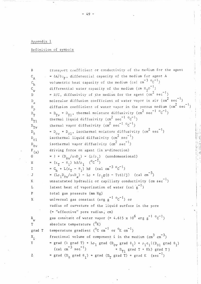
- 49 -
Appendix I
Definition of symbols
B
CA
ch c
w D
D a
D p
DT
DTl
DTv
De
DOl
Dev
F (x)
G
H
I
J
K
L
p
R
R w
T
grad
X. ]_•
y
z
T
truns~ort coefficient or conductivity of the medium for the agent
= 6A)5l~, differential capacity of the medium for agent A -3 0 -1
volumetric heat capacity of the medium (cal ern C )
differential y,rater c2pacity of the medium (ern H?O-l) ~ ') -]
= 13/C, diffusivity of the medium for the agent (ern~ sec ) 2 -]
molecular diffusion c6efficient of water vapor in air (em sec ) 2 -1
diffusion coefficient of water vapor in the porous medium (em sec ) . d'ff . . ( 2 -1 oC-1) = DTv + DTl' thermal rn?1sture 1 us1v1ty ern sec
. . d. ff . . ( 2 -1 0 -1) thermal l1qu1d 1 us1v1ty ern sec C
d . f f . . ( 2 -1 oc-1) thermal vapor 1 us1v1ty ern sec
= DGv + D81 , isothermal moisture diffusivity
isothermal liquid diffusivity (crn2 sec- 1)
. l d. ff . . ( 2 - 1) 1sotherma vapor 1 us1v1ty em sec
driving force on agent (in x-direction)
1 + (D8v/avDa) - (~/~l) (nondornensional)
(t:T - e1) hB/pl ( C )
2 -1 (ern sec )
~ + L(t:T- e1
) hB (cal crn- 3 °C- 1)
(Lp1D8v/avDa) - Lp + {p 1g(~- Ty~)/j} (cal cm-
3)
unsaturated hydraulic or capillary conductivity (ern sec- 1) ' -1 latent heat of vaporization of water (cal g )
total gas pressure (mm Hg) -] 0 -]
universal gas constant (erg g C ) or
radius of curvature of the liquid surface 1n
(="effective" pore radius; ern)
the pore
gas con;ta~t of water vapor (= 4.615 x 10⁶ erg g-I 0 c- 1)
b 1 ( OK) a so ute temperature
temperature gradient (°C em-] or °K crn- 1) 3• -3 fractional volume of component i 1n the medium (ern em )
=grad (A grad T) + Lp 1 grad (Dev grad e1) + p1c 1{(D81 grad e1
)
(Cal ern- 3 sec-. I ) D d T Kk) d } + Tl gra + - gra T
grad (D 8 grad e1
) +grad (DT grad T) +grad K (sec- 1)

e, e
e s
g
grad
h
J
k
k. l
X
X 0
X m
X q
z
- 50 -
3 -3 = c, volumetric a1r content of the medium (em ern ) -] 0 -]
specific heat of liquid water (cal g C )
part i a 1 v a p 0 r pressure of ~\rater in u n i t s u f mr:; li g :1 r, d -?
dyne ern ~ respectively
s a t u r a t ion v a p o r ? res sure of \.J ate r ( mm H g) -?
acceleration due to gravity (= 981 em sec ~) -]
gradient (ern )
fractional relative humidity (nondirnensional)
mechanical equivalent of heat (= 4.18 x 10 7 erg cal-l)
unit vector in the vertical upward direction
ratio of the average temperature gradient in component i and
the corresponding quantity in the continuous medium, in \.Jhich
component i is dispersed (i.e. air or water, nondimensional)
flux density of agent A (in x-direction, units of transported -? -]
agent em ~ sec ) -2 -1
heat flux density (cal ern sec ) -2 -1
flux density of water in the liquid phase (g ern sec ) -2 -] = qv + q
1, total moisture flux density (gem sec )
-? -) flux density of water vapor (g ern - sec )
time (sec)
horizontal coordinate (ern)
fractional volume of organ1c matter (cm3 crn-3)
fractional volume of soil minerals other than quartz
f · 1 1 f · l ( cm3 em- 3) ract1ona vo urne o quartz part1c es
vertical coordinate, positive upHards (em)
3 -3 (ern em )

0.
,)
y
f (.:.)
A
A a
A app
A. l
A q
A v
\)
p
lJl· F
- 51 -
tortuosity factor allowing for the extra p<JLiJ J t·ngth (nondimensiono1)
,. - I -T ( - 3 0 c- 1 ) o~ 0 o g ern
(l/o) (6o/6T) (°C- 1)
3 -3 a, volumetric a1r content of the medium (ern ern )
D /D , ratio of diffusion coefficients (n0ndimensional) p 3 3 -3
total porosity of the medium (ern em )
= (gr~d T)3/grad T, ratio of average temperature gradient in
air-filled pores to the overall tem~.H~: rat ure g r :1 di en t (nond irnens ion2.l) 3 -3,
= ::v + :.\, totul volumetric moisture content,__-,£ the medium (em err: )
v3lue of e1
at v.r~ich "liquid continuity" fails (crn3
cm-3
) 3 -3
volumetric liquid content of the medium (ern ern )
volumetric vapor content of the medium (cm3 cm- 3)
overall thermal conductivity of the medium (cal cm-l sec-l °C- 1) -] -1 0 -1
thermal conductivity of dry a1.r (cal em sec C )
= A + A apparent thermal conductivity of air containing water a v' -] -1 0 -1
vapor (cal em sec C )
thermal conductivity of component 1. 1.n the medium (cal cm-l oc-])
-1 sec
-1 -1 0 -1 thermal conductivity of the continuous medium (cal em sec C )
apparent increase of the thermal conductivity of air due to vapor
diffusion (cal cm-l sec-l °C-l)
= P/(P-e), a mass flow factor to allow for the mass flow of water
vapor arising from a difference in boundary conditions for the air
and water vapor components in the medium (mm Hg- 1)
factor ; 1 arising from vapor flux enhancement mechanisms
(nondimens ion a l) -3 density of water vapor (g em )
density of (liquid) water ( g cm- 3) -3
density of saturated water vapor (g em ) -I
surface tension of water (dyne em )
matric potential of the moisture in the medium, in units of em -1
_H 2o and erg·g respectively (negative 1.n unsaturated media)
partial potential' of the agent related to driving force F
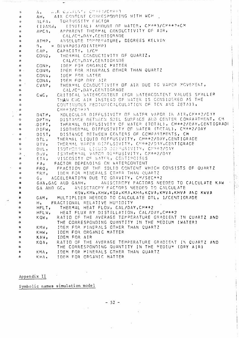
·:r.
* *
* * * * * * * * * * * * * * * * * * * * .•. ...
, I~ 1
1\H, :\ L F ,\,
J·~ ~ R L .J . , i :_ ! .. r : C :' i ,:. ~ I C : ... :.;: <= l A I R C r; ~·!T [ r·~ T C I') ;n.! C ~ P 'J~ J r; IN G ~·J I T H h' C f.l
1 u r~ T ' J n s r T Y r :1 c T o n ( I ) f1 ~L·J , 1\PC A,
r r~nr r ,\L) M·:nunr nr- 1·/ATE~., c~-:n:t1/Cf'I**?=C~
1\PP!\RE~~T THEP.~~L COt\GLCTIVi1Y Of AIR,
/\ T t-.1 P , f', CAP, COt~Q,
CONH, CON t·1, CON\~,
CONA, CVI\P,
CrJC,
DAT M, OPT H, .0 IF T, OIFW, DIST, OTL, DTV, 0\·:L 1
[) :1 v ' E T .t\ , FA, FRQ,
C /\ L I C • ~ , n A Y , r. E N T I G n. td) E r\ ;\ S ~; L U T E T r~ ~~ n F. r: i1 T U q E , 0 E G R E E S K (LV I N
= O(VAPOS)/D(hTEMP) C A r ,\ C I T Y , l/ C tJ
T H E ~~ !'-~ /\ L C r: ~ C U C 1 I V T T Y 0 F Q U fl R T Z , C .\ L I C .'·1 , n ,\ Y , C E ~; T I G ~~ 4 D E
I i) t t' F rJ R G R G !J ~l I C ~ f. T T E R I n E t·l F !l R ,'-1 f N E R /\ L S 0 THE R T H 1\ N Q U ,\ P. T l I DE tJ F r; I{ \·, /\ T F.: R T fJ F. ~·~ F iJ P n R Y j I R THERMAL CC~CUCTIVITY OF AIR DUE TG VAPCR ~GVE~E~T,
C A L I C t.• , D ,\ Y , C F: N T I G P, J\ D E C t-~ I T I C /d_ ':1 ·~ T E ~~ C G ~; 1 E t J T { F C R ',-; !\ T E R C 0 :-~ T E t'\ T V fl L U E S S I .A () L l E R THAN C'riC ldP. Il''>STEtD OF 1.-i~i~R IS CC~~SIDr::RED /IS THE C fJ ~.; T I ;-: U r; U S ,'-' E 8 1 U ;.' { C .~ L C U L j T I 0 ~ 0 F T C :\ A ~ C Z E T ~~ ) l , c •'·\ ;!: ):( 3/ c.',;;,·:( l
,Y, 0 L E C U L /. ~ 0 I F F C S I 'J I T Y D ~ \ ·, t ... T F q V ;\ P C R I i\ /i I l , C l' * ~ 2 I C .~ Y D I S T .\ ": C E R t T ':; t: r: .'~ S c: I L S U ~·~ F .~ C;: A i: I) C E :·~ T E ['{ C 0 M !==A ~ T ~·'·F. NT , C '~ T H != P. ~' A L n I F F L S I V I T Y C F \\ A T E R { T 0 T .~ L ) , C M * * 2 I D /! Y , C E t\ T I G R A 0 l I S 0 T H E ::t '·~ A L 0 f F F U S 1 V I T Y C r •,.; tl T f. R { T ~ T .\ l ) , C ""· * * 2 I D 1\ Y o r s r A t-J c '= e F r h E E ,~J c r: i·, r E q s o F c c M P ,~ ~~ T tJ F. t\ T s , c M
T H f R ~1 A L L I Q U I f) Q I r- F U S [ V I T Y , C t~ * * 2 I D ;) Y , C E NT r G R A 0 E 7 H E P, '·1 t\ L V ,\ P C' R G ~ :-: F L S ! V I T Y , C ~ ~ 1~ * 2 I D \ Y , C 1: ~i T I G R A C E
TS:lTHf:P.''t,\l V.~\~l:~ :Ji::F=USIVITY, C:i'*~?./D'l.Y 1} I S C C S I T Y C c ~\ ,'\ T r~ R. , C F:: :~ ~ I 9 C I S E S
FACTOR OEPE~OI~G CN hhTEqCONTENT FPACTIO~ OF THE SOLID CSNTENT WHICH CO~STSTS OF QUARTZ
* FR~, IOEM FOq MI~ERALS CTHF~ TH~N QUARTZ * G, ACCELERATinN DUE TC Gn~VITY, C~/SEC**2 * G A 'A , G ,\ C ,.\ n D G /u\ H , .\ N I S C T R r: P Y F A C T 0 R S N E E 0 E 0 T 0 C tJ L C U L AT E K A W * GA ~-~NO GC, ~~<JISCTRCPY FACTOPS "JEEOF:f) T~ C.'\LCUL.hTF. * KQW,KM~,KHW,KQA,KM~,KH~,KCVA,KMVA,KHV~ ~~C KWV~
* GAM, MULTIPLIER NEEDED TO CALCULATE DTL, 1/CE~TIGR~DE
* H, FRACTION.£\l RELilTIVE HU".IOITY * HFLT, THERMAL HEAT FLOW, CAL/DAY,C~**2 * HFLW, HEAT FLUX RY DISTILLATION, CAL/QjY,CM**2 * K Q W , R AT I 0 C F T H E ;1 V E R A G E T E ~~ P E R A T U R E G ~ '\0 I E f\ T T N C U !l R T Z A N 0 * THE CORRESPONDING QUtdJTITY IN THE ~EDIUM CWATERl * KMW, IDEM FOR ~INER~LS OTHER THAN QUARTZ * K H W , I 0 E f·~ F 0 !\ 0 R G A N I C M ~ T T E R * KAW, IDEM FOR AIR * KQA, RATIO OF THE AVERAGE TEMPERATURE GRADIE~T I~ CU~RTZ AND * THE CORRESPONDING QUANTITY IN THE ~EDIU~ <DRY AIRJ * KMA, IDEM FOR MINERALS GTHER THAN QUARTZ * KH~, IDEM FOR ORGANIC MATTER
Appendix II
Symbolic names simulation model
- 52 -
)~ K \..JV ~~, g t~ I l 0 () F l H 1: /.l. V r; t~ A G E T E M P E R /\ T U P. E G R A G ( 1: r ~ r l N W A T E R A N 0 iHE CC,RI-:=SPO!JI~UJG QUAt~Tli'( 1N lHE MEDIUI" (AlR(-+HATER
VAPOR))
* K Q V 1:1 , I I I E H i: I J R Q l J /~ R 1 7. ~ K ~~ V A , I ! :• F M F i K M I 1\1 E R A l S C T H E R T H A ~J Q U A R T Z ;'c \\HVA, 1Dt:H FDH rJP.GANIC HATTeR ;c L , L 1\ T E i~ T HE :~ T CJ F V A r 0 R I 7. t\ T l D ~J 0 F vJ/4 T E R , C ,1L/ G !~A f1
f''1C., C(Jifff:f~T CJF i·\I iJE~I .. LS OTHER THP.tJ QUAHT Z 1 CM};:*3/(t.J~ 1~t.<3
IJ., VI~:;(:;JSfTY Or- \-lt-.TE.i~ .)T .~0 CEGr~E:S CELCIUS, CENTIPOISF.S O>i C , 0 ~ G ;~; Jl C :-\..\ T I~ ~~ C G 1'-! T ~ lJ T , C H.:.:.;: 3/ C 11 ~: ~ '3
~' P , S L C T it l i J, C 1·1 * POR, POROSITY, CM**3/CM*~3 ;;: P R t S , T 0 T ~ L G A S P R :: S S U R. :: , H H H G 1;' P U AN 0 P L , S U C T r 0 N V ~ L lJ E S U S E 0 i t.J T H E C A L C U L A T I C t\ C F T h E S L C P E * n I= THE S U C T r 0 ~J- vJ ).\ T E R C G NT E t\ T CURVE ,:, R t G 1\ S C 0 1"1 S l" A i I T 0 f vJ A T E H V A r n ::\ , C R G I C P. 1i I·~ , K E l V I N * RPER, RECIPROC~L VALUE OF THE PERIOD OF THE SINUSOIDAL * TEMPERATURE VARIATION, 1/0AY * Q C , Q U l~ r~ T .?: C 0 UTE;\! T 1 C '-' <: ~:: l / C I·~::~.·,~ * S 0 L C , S I) L I D C IJ IJ TENT , c.·,~-'~::{ J I C i·1 ~:; :~ 3 * SP, SLOPE OF THE SUCTIOi\-~·1/\TEHCO;,~TENT CURVF:,CM**4/Ct1**3=Cl-' * T A r\ P , A ~., P L I T U n E 0 F T H E T F '-' P E R A T U :{ E \1 /~ V E , C E N T I G R A 0 t S * TAV, AVERAGE TEMPERATURE OF THE TEMPERATURE WAVE, CENTIGRADE$ * TCOM, THICKNESS CC~PARTMENT, CM * TCN, THERMAL CONDUCTIVITY, CAL/C~,OAY,CENTIGRACE
* TCND, THERMAL CONDUCTIVITY nF DRY SOIL (WATERCONTENT * EQUALS ZERO), CAL/CM,OAY,CENTIGRACE * TCNL, LO~·JER LI!·1fT THER,'·':\L CfJNOUCTIVITY RANGE CALCULATED :¢t W I T H ~,1 A T E R A S T H E C 0 N T 1 N U 0 US tJ. E 0 I U M * ( 1lTEMP, £INITIAL) TEMPERATURE, CENTIGR60ES * TNHF, TOTAL NET HEAT FLOW, CAL/DAY, CM**2 * TN~~F, TOT:~l NET hATER FLO~·l 7 Ct~/OAY
* V, MASS-FLC~ FACTOR * VAPD, DENSITY OF ~ATER V~POR,GRAM/C~**3
* V P D S,. 0 E i'·J S IT Y 0 F SATURATE 0 \·1 ATE P. VA PC R * (J)VHCP, (INITIAL) VOLU~ETRIC HEAT CAPACITY,
* * * * * * * * * * ~
* * * *
CAL/CM**3,CENTIGRAOE ( I) V HTC, (INITIAL) VOLUMETRtC HEA1 CONTENT,
CAL I CM~'* 2 ( I l we, HCH,
WCN, \<JCON, WCU AND
't1DEN, WFLT, 'rlfLW, lETA,
(INITIAL) WATERCONTENT, CM**3/CM**3 WATERCONTENT WHERE THE VALUE FOR THE RELATIVE HUMIDITY IS ABOUT o.sqo {P ABOUT 15000 MEAR) HYDRAULIC CONDUCTIVITY, C~/D~Y
HYDRAULIC CON~UCTIVITY 4T 20 DEGREES CELCIUS, CM/OAY WCL, WATERCONTENT VALUES USED IN THE CALCULATION OF THE
SLOPE OF THE SUCTTON-WATERCONTENT CURVE DENSITY OF {L1QUID) WATER, GRA~/CM**3 THERMAL WATER FLOW, C~/OAY
ISOTHERMAL WATER FLOW, CM/OAY RATIO OF TE.~PERATURE .GRADIENT IN AIR-FILLED PCRES TO OV~R~LL JEMPERATURE GRADIE~T
Appendix II (continued)
- 53 -

- 54 -
References
A .. ~ONYHOUS (1967-1968) - CSHP User's Hanual. IBH Ne\·.7Sletter H20-0367-2.
BOLT, G.H., A.R.P. JA..~SE and F.F.R. KOENIGS (1965) -Syllabus Kandidaats
college Algemene Bodemkunde, deel 2 Bodernnatuurkunde.
BURil~GH, P. ( 1968) - Introduction to the study of soils in tropical and
subtropic?l regions. Pudoc, ~ageningen.
CARY, J.\.J. and S.A. TAYLOR (1962a)- The interaction of the simultaneous
diffusion of heat and \.Jater vapor. Proc. Soil Sci. Soc. Am. 26, 413-416.
CARY, J.\.J. and S.A. TAYLOR (1962b) - Thermally driven liquid and vapor
phase transfer of \·.7ater and energy in soil. Proc. Soil Sci. Soc. Am. 26,
417-420.
CARY, J.hT. (1965)- h7 ater flux in moist soil: thermal versus suction
gradients. Soil Sci. 100, 168-175.
CARY, J,\.J, (1966) -Soil moisture transport due to thermal gradients:
p r act i c a 1 asp e c t s . P roc . S o i l S c i . Soc . Am. 3 0 , 4 2 8- 4 3 3 .
CASSEL, D. K. , D. R. NIELSEN and J. \.J. BIGGAR (I 969) - Soi 1 water movernen t 1n (.·-.·
response to imposed temperature gradients. Proc. Soil Sci. Soc. Am. 33,
49 3-500.
FRITTON, D.D., D. KIRKHAH and R.H. SHAH (1970) -Soil water evaporation,
isothermal diffusion, and heat and water transfer. Proc. Soil Sci. Soc.
Am. 34, 183-189.
GOUDRIAAN, J. and P.E. WAGGONER (1972) - Simulating both aerial microclimate
and soil temperature from observations above the foliar canopy. Neth.
J agric. Sci. 20, 104-124.
HADAS, A. (1968) -Simultaneous flow of water and heat under periodic heat
fluctuations. Proc. Soil Sci. Soc. Am. 32, 297-301.
JACKSON, R.D. (1964)- \.Jater vapor diffusion in relatively dry soil. III
steady-state experiments. Proc. Soil Sci. Soc. Am. 28, 467-470.
JACKSON, R.D., D .. A .. ROS.E and H.L. PEl'TI'1Al~ (1965) - Circulation of \,'ater 1n
soil under a temperature gradient. Nature 205, 314-316.
KElJLEN, H. VJ.ili and C.G.E.H. VANBEEK (1971) -Hater movement 1n layered
soils. 1. A simulation model. Neth. J. agric. Sci. 19, 138~153.
KRAMER, P.J. (1969)- Plant and soil water relationships. McGraw-Hill,
New York.
LETEY, J. (1968) - Hovement of water through soil as influenced by osmotic
pressure and temperature gradients. Hilgardia 39, number 14, 405-418.

- 55-
OO~ffiN, G.J.M. and G.J. STARING (1972) - Verslag ingeni~urs?raktikum,
afd. Landbouwscheikunde.
PHILIP, J.R. and D.A. DE VRIES (1957) - Noisture movement 111 porous
m3terials under temperature gradients. Trans. Am. geo?hys. Un. 38,
222-232.
ROSE, C.\v. (1966) - Agricultural Physics. Pergamon, Oxford.
ROSE, C.~. (1968a) - Water transport in soil with a daily temperature wave:
Part I. Theory and experiment. Aust. J. Soil Res. 6, 31-44.
ROSE, C.H. (1968b)- \~ater transport in soil ·h1 ith a daily tem?erature wave:
Part II. Analysis. Aust. J. Soil Res. 6, 45-57.
ROSE, C.h'. (1968c) - Evaporation from bare soil under high radiation
conditions. Int. Congr. Soil Sci. (Trans. 9th, Adelaide, Australia) 1,
57-66.
RIJTEt~, P.E. (1969) - Soil moisture forecasting. Nota 513, Institute for
Land and Water Management Research.
SLATYER, R.O. (1967) -Plant-water relationships. Academic Press, London.
STROOSNIJDER, L., H. VAN KEULEN and G. VACHAUD (1972) -Water movement in
layered soils. 2. Experimental confirmation of a simulation model. Neth.
J: ag ric. Sci . 2 0 , 6 7-7 2.
TAYLOR, S.A. and J.W. CARY (.1960) -Analysis of the simultaneous flow of
water and heat or electricity with the thermodynamics of irreversible
processes. Int. Congr. Soil Sci., (Trans. 7th, Madison, Wise.) 1, 80-90.
TAYLOR, S.A. and J.W. CARY (1964) - Linear equations for the simultaneous
flow of matter and energy 1n a continuous soil system. Proc. Soil Sci.
Soc. Am. 28, 167-172.
VRIES, D.A. de (1952) -Ret warmtegeleidingsverrnogen van grond. Med.
Landbouwhogeschool, Wageningen, 52, 1-73.
VRIES, D.A. de (1958)- Simultaneous transfer of heat and moisture 1n porous
media. Trans. Am. geophys. Un. 39, 909-916.
VRIES, D.A. de (1963) - Thermal properties of soils, p. 210-235. In:
W.R. van Wijk (ed.), Physics of plant environment. North-Holland
Publishing Co., AmSterdam.
WIERENGA, P.J. and C.T~ DE WIT (1970) - Simulation of heat transfer 1n soils.
Proc. Soil Sci. Soc. Am. 34, 845-848~
WIT, C.T. DE and H. VAN KEULEN (ed.) (1970) -Simulation of transport
processes in soils. Report No~ 1, Department of Theoretical Production
Ecology, Agricult~ral University, Wageningen, The Netherlands.
WIJK, W.R. VAN and D.A. DE VRIES (1963)- The atmosphere and the soil, p.
17-61. In W.R. van Wijk (ed.), Physics of plant environment. North-Holland
Publishing Co., Amsterdam.

initial volumetric
absolute change*) in initial volumetric moisture content (%) for compartment moistur'e (%) time content (days) 1 2 3 4 5 10 15 20 21 22 23 24 25
(-) ( +) (+) (+) (+) (+) (+) (+) (+) (+) (+)
5.00 0.025 • 1 9 .04 .03 .03 .02 .• 01 X X X X X X X
0.05 .29 .04 .03 .03 .03 • 01 .01 X X X X X X
0.075 .36 .05 .03 .03 .03 .02 .01 X X X X X .01
0. 10 .43 .06 .04 .03 .03 .02 .01 .01 X X X X .03
0.20 .65 .09 .04 • Ol~ .03 .02 .02 .01 .01 . 01 X X • 1 5
0.30 .86 • 13 .03 .04 .03 .03 .02 .01 .01 . 0 1 X X .30
0.40 1 . 06 . 1 8 .03 .04 .03 .03 .02 • 01 . 0 1 .01 X X .45
0.50 1. 28 .24 .02 .04 .03 .03 .02 .01 • 01 . 01 X X .61 ••- r • • • ·• - •
(-) (+) (+) (+) (+) (+) (+) (+)
10.00 0. 025 . 1 5 .03 .02 .02 • 0 2 .01 X X X X X X X V'l 0'\
0.05 .23 .03 .03 .02 .02 . 01 X X X X X X X
0.075 .28 .03 .03 .02 .02 .01 . 01 X X X X X • 0 1 () . 1 0 .33 .03 .03 .03 .02 .02 . 01 X X X X X .03 0.20 .49 .03 .03 .03 .02 .02 .01 X X X X X . 14
0.30 .63 .03 .03 .03 .02 .02 . 01 X X X X X .26 0.40 .77 .03 .03 .03 .02 .02 . 01 X X X X X .38 o.so· .90 .03 .03 .03 .02 .02 . 01 X X X X X . 51
.....
;:) (-) = decrease (+) = increase
X = no change
Table 2 Spatial and temporal variation of the volumetric moisture content after imposing a temperature gradient (25°C-15°C) for different initial water contents (homogeneous soil column having a length of 25 em). Suction and hydraulic conductivity curves used are those of an unplowed light humous sandy soil (van Keulen and van Beek, 1 971 ) .
------ - ---- -

initial volumetric absolute change:t:.) in initital volumetric moisture content (%) for compartment moisture (%) time content (days) 1 2 3 4 5 10 15 20 21 22 23 24 25
(-) (-) (t) (t) (t) (t) (+) (t) (+) (t) (+) (+) (+) -~ () . ;_) 0 0.025 . 1 0 .02 . 01 .02 .02 .01 X X X X X X X
(-)
0.05 . 12 .05 . 01 . 01 .02 . 0 1 X X X X X X X
0.075 • 13 .07 .02 X .02 .02 . 01 X X X X X • 01 (-)
0. 10 . 1 3 .08 .04 . 01 . 01 .02 . 01 X X X X .01 .02 (-)
0.20 . 14 . 1 0 .07 .04 .02 .02 . 0 1 . 01 .01 . 01 .02 .04 .07 0.30 :1 5 . 12 .09 .06 .04 .01 . 01 .01 .02 .03 .04 .07 . 11 0.40 . 17 . 14 . 1 0 .08 .05 . 01 . 01 .02 .03 ,05 .07 . 1 0 • 14 0.50 . 18 . 1 5 . 12 .09 .07 X . 01 .03 .05 .06 .09 . 12 . 17
(-) (-) (-) (-) (-) (+) (+) (+) (+) (t) (+) (+) (+) ln .........,
35.00 0.025 .05 • Ot+ .03 .02 . 01 .02 . 01 X X X X X X
0.05 • o5· .05 . 01+ .03 .02 . 01 .02 . 01 . 01 . 01 .01 .01 . 0 1 . 0.075 .06 .05 .04 .04 .03 X . 01 .02 .02 .02 .02 .02 . 0 2
(-) 0. 10 .06 .05 .04 .04 .03 . 01 .01 .02 .03 .03 .03 .03 .03 0.20 .06 .05 .05 .04 .04 . 01 . 01 .03 .03 • 0L~ .04 .05 .05 0.30 .OG .05 .05 .04 .04 .02 . 01 .03 .03 • Q!~ .04 .05 .05 0.40 .06 .05 .05 • O!.J- .04 .02 . 01 . 03 .03 .04 .04 .05 . 0 5 0.50 .OG .05 . Q5 .04 .04 .02 . 0 1 .03 .03 .04 .04 .05 . 0 5
~) (-) = decrease (+) = increase
X = no change
Table 2 (continued)

initial volumetric
absolute change*) in initial volumetric moisture content (%) for ·compartment moisture time content ( 06) (day;;) 1 2 3 4 5 10 1 5 20 21 22 23 24 25
-- -··
(-) ( +) (+) (+) (+) (+) (+) (+) (+) (+) (+) ( +) :! . 00 0.025 .54 • 12 .09 .07 .06 .02 X X X X X X :-:
(a) 0.05 .83 . 15 . 1 0 .09 .08 .04 . 0 1 X X X X X • 01 0. 075 1 . 0 5 . 17 • 1 1 . 1 0 .09 .05 .02 . 0 1 . 0 1 • 91 X X .04 0. 10 1. 24 . 19 . 1 1 . 10 .09 .05 .03 . 01 . 01 . 01 • 01 X .08
(-) (-) (+) (+) (+) (+) (+) (+) (+) 5.00 0.025 . 10 . 01 .02 .02 .02 . 0 1 X X X X X X X
0.05 . 1 2 . 01} X .02 .02 . 01 X X X X X X X (b) (-)
0.075 . 13 .06 . 01 . 01 .02 . 01 . 01 X X X X X . 01 0. 1 0 . 14 .07 .02 X . 01 . 01 .01 X X X X .01 .02
(-) ( +) (+) (+) (+) ( +) U1 co
20.00 o.n?.s . 12 .01 .02 .02 .02 . 01 X X X X X X X
(b) (-) 0.05 . 16 .02 .02 .02 .02 .01 X X X X X X X
~) (-) = decrease (+) = increase
X = no change
Table 3 Spatial and temporal variatign og the volumetric moisture content after imposin8 a thermal gradient. (a) Temperature gradient: 35 C-5 C
Suction and hydraulic conductivity curves are the same as for Table 2. (b) Temperature gradient: 25°C-15°C
Suction and hydraulic conductivity curves refer to a plowed humous sandy soil (van Keulen and van Beek, 1 971 ) .
------ ----~---- -----~---- ---------

initial volumetric moisture content C'o)
5
10
20
35
soil type
unplowed lit;ht humous sandy soil
plowed light humous sandy soil
unplowed light humous sandy soil
"
plowed light humous sandy soil
unplowed light humous sandy soil
thermal vapor diffusivity
DTV -· -
2 -1 0 -1· (ern day C )
2.4 X 10 -2
2.0 X 10 -2
2.2 X 10 -2
2.1 X 10 -2
1.9 X 10 -2
1.2 X 10 -2
thermal liquid diffusivity
DTL .. - ·-. --- ---·
( em 2 day - 1 ° C - 1 )
1.1 X 10 -8
3.7 X 10 -4
0.9 X 10 -8
1.7x10 -3
1.1 X 10 -3
0. 1
isothermal vapor isothermal liquid diffusivity diffusivity
DWV DWL ...
2 -1 (em day )
2 -1 (em day )
2.2 X 10 -2
3.2 X 10 -5
9.5 X 10 -1 13.5
2.1 X 10 -2 3.6 X 10 -5
8.5 X 10 -3 25.0
1.6 X 10 -4 6.4
7.5 X 10 -5
1000
Table 4 Rough values (at 25°C) for the thermal and isothermal moisture diffusivities'at different volumetric moisture contents.
Ln \D
I
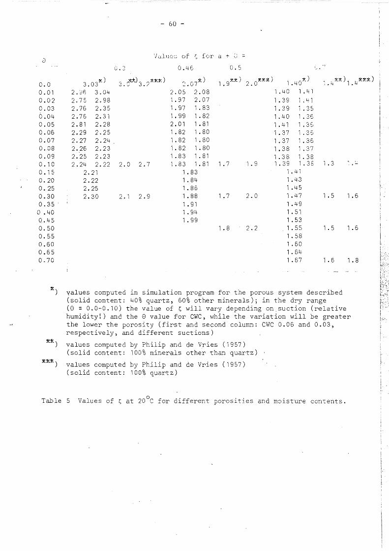
- 60 -
'/oluo:::. of r;, for a + ,,
= \j
0 0.3 0.45 0.5 ~~ . ~:
0.0 3.03~) 2. ct+..) 3. ?~!Y.~) '2.07:t) 1 . 9 :t:t ) 2.0:t:t~) 1 .40:*:.) ' .. :t.*-. ) 1 4 :t.:r.:t) I • 4 •
0. 01 2.~f) 3.04 2.05 2.08 1. 40 1 . 4 l
0. 0 2 2. 75 2.98 1. 97 2.07 1 • 3 9 1 • 41 0.03 2.76 2.35 1. 97 l. 83 1 • 39 1 • 3 5 0.04 2. 76 2.3i 1. 99 1 . 82 1. 40 1 • 36 0.05 2.81 2.28 2.01 1 . 8J 1 • 41 1 . 3 6 0.06 2.29 2.25 1 • 82 1 . 80 i . 37 1 . 3 6 0.07 2. 27 2.24 1. 82 1. 80 1 • 37 1. 36 0.08 2.26 2.23 1. 82 1 • 80 1 • 3 8 1 • 3 7 0.09 2.25 2.23 1 • 83 1 • 81 1 • 3 8 1 . 38 0. 1 0 2.24 2.22 2.0 2.7 1 • 83 1 • 81 1 • 7 1.9 1 • 39 1 . 3 s l . 3 '.-0.15 2.21 1.83 1 • 41 0. 20 2.22 1 . 84 1. 43 0. 25 2.25 1 • 86 1 • 45 0.30 2.30 2. 1 2.9 1 . 88 1 • 7 2.0 1. 4 7 1 • 5 1 • 6 0. 35 . 1 . 91 1 • 49
0 • 40 1 . 94 1 • 51 0 .. 45 1 . 99 1 . 53 0.50 1 • 8 2.2 1 . 55 1.5 1 . 6 0.55 1.58 0.60 1 • 60 0.65 1. 64 0.70 1 • 67 1 • 6 1 • 8
~) values computed in simulation program for the porous system described (solid content: 40% quartz, 60% other minerals); in the dry range
:t:t)
:tx:t)
(0 = 0.0-0.10) the value of swill vary depending on.suction (relative humidity!) and the 0 value for ewe, while the variation will be greater the lower the porosity (first and second column: ewe 0.06 and 0.03, respectively, and different suctions)
values computed by Philip and de Vries (1957) (solid content: 100% minerals other than quartz)
values computed by Philip and de Vries (1957) (solid content: 100% quartz)
Table 5 0 Values of s at 20 e for different porosities and moisture contents.

47.5 1. 80
173 2.07
~) (-) =decrease ( +) = increase
x = no change
time interval
(days)
0.01
0. 1
0. 5
0.01
0. 1
0.5
- 61 -
:K absolute change ) in % volumetric moisture fGr·
compartment
(-)
.08
. 51
1 • 2 5
(-)
.07
.34
.88
2 3
(+)
.05
.09
.06
(+)
.02
.03
.02
(+)
.02
.08
. 10
(+)
.02
.03
.03
4 5 20 25
(+)
. 01
.07
.09
( +)
. 01
.03
.03
(+)
X
.06
.09
( +)
. 01
.03
.03
(+)
X
X
.02
(+)
X
X
. 01
( +)
X
X
0. i 6
(+)
X
.02
.46
Table 6 t·1oisture distribution corresponding with Figure 11.

- 62 -
Sur.~ totals ( e:•q.)r··::ssed as absolute vo~umetr·ic % r;: .. :.•. r_:'.:.,f::pu.r·tHJ0[;t
· of 0. 8 em) of decr·eases (-) and incr·eases ( +) e-i ., : _;::/:;tr·ic r;1cisturoe lrltegr'ation , cont~nt thr'oughout the column due to a th~rmGtl gr··..1 ~~ ~:·;t ( 25°C-15°C) method ~after 0.5 day of ~imulation for initial volumetric ~0isture content (%)=
I I
5.00 10.00 20.00 3~.00 I
! i
6 tJ t
NILNE j ~it 2 5 +1.24 -O.Oi -1 • 1 s +0.97 -o. 18 -0.74 +0.41 -0.33
I
I '"'i .25 "\<i ,25 i -0.77 +0.70 -0.07 -0.60 +0.52 -0.08 RKS -0.40 +0.31 -0.09
i -1.28 +1.27 =0.01 =0.90 +0.83 =0.07 -0.72 +0.64 =0.08 '
Comparison of METHOD MILNE with METHOD RKS
Initial volumetric DTV DTL DI'IV DWL
(em 2 -1 oc- i) 2 -I oc -I) 2 -1 2 _,
moisture content ( \) day (em day (em day ) (em clay )
4.5 2.7 X 10⁻² 9.5 X 10- 4 3,6 X 10⁻³ 12.3
9.0 2.6 X 10⁻² 1. 5 X 10- 3
·· 6. 6 X 10-lf 13.0
1'6. 0 2,5 X 10- 2 3.3 X 10- 3 i.i X 10-4 10.0
Table 8 0 Rough values (at 23 C) for the thermal and isothermal moisture diffusivities at different volumetric moisture contents.

initial volumetric initial volumetric initial.volumetric j moisture content: 5% ; moisture content: 12% i moisture content: 20% i simulated period: 0. 1 day ! simulated period: 0. 1 day ; simulated period: 0. 5 day
1 L-----·--------··· ------·---····-----.---'--------.. - ... ·-· ............. ---- ._ . - .... - .... ____ ..__ __ .............. ---· ------------------! o I ! temperature ( C) I l !
- - • w' "' -- ·- . - - ·- ~- -- ~-- .. I
compartment j- -- - --:· . l m1n1mum maximum minimum maximum : minimum maximum
2 5
10 15 20 25
2 5
10 15 20 25
I 5.70 I 6.99 I , o. 28 I I
I I I
I
14.22 15.00 14.99 15.00
~- --- minimum
i 4.75
I I I
! i
4.93 4.97 4.99 5.00
I 5.oo L ___ 4._99
24.36 23.23 20.34 16.43 15.24 15.07 1 5. 01
maximum
5.17 5.04 5.03 5.01 5.00 _5. 00 5.00
7.40 1'0.58 14.15 14.99 15.00 15.00 15.00
22.91 20.06 16.47 15.25 15.09 15.04 15.00
volumetric moisture content (%) ...
minimum maximum
11 • 9 5 12.01 11 • 99 12.02. 11 • 99 12.00 12.00 12.00 12.00 12.00 12.00 12.00 12.00 12.00
i
...
I
I
i
7.57 10.85 14.27 14.96 15.00 15.00 14.99
22.73 19.78 16.27 15. 19 15.07 15.03 15. 01
. - -- ~ ·- --- . - - --·--- -
- -- - ... ·-·- - - .. -·- -- -·-
minimum
19.96 19.97 19.98 19.98 19.99 19.99 19.99
maximum
20.02 20.01 20.00 20.00 20.00 20.00 20.00
Table 9 Temperature and moisture content yariation generated in soil column by a sinusoidal variati0n at the left side for different initial volumetric moisture contents. I ' 'l 1° . . 1° . d f n1t1a temperature: 5 C; average temperature s1puso1dal wave: 5 C; ampl1tu eo tcmpcratur~
wave: 10°C; period of temperature wave: 0.01 day; right side of column kept at the initial temperature (FUDGE= 1.).
"" . VJ

TS
I I
'..... ~------------- -- - -
-----
HF I LT{J)
...__ ____ - ----
DPTH(I) I
I - 1
AW AT AV AV AD
WF WF tlf ._If.'
-
i
CN(I~ CN(I DW(I) DT(I) WV(I)
LT(I) WF LW(I) WF
~~~~J HF HF
~
NWFT(I), NWFW(I) TNWF(I)-NHFT(I), NHFW(I) TNHF( I) ·· . '
IAMW(I), AMW(I) IWC( I) , WC ( I )
.·
IVHTC(I), VHTC(I) IVHCP( I); VHCP(!) · ITEMP( I)·, TEM.P( I) ATMP(I) WCON( I), .. WCN( I) ETA(I), TCN(I) P(I), FA(I), A(I), H(I) CVAP(I), APCA(I) DATM(I), ZETA(I) CAP (.I) , V APD ( I) DTL( I), DTV (I} FHFT(T) DWL(I), DWV(I) DIFW(I)
I
I
LT~I+l~ LW I+-1 LT I+l LW I+ . -
I t 1
--------..,
TEMP(26)
HFjLT(26
________ __,
NL (::25)
Fig. 1 Schematic representation of the geometry of the system (homogeneous porous column) and main symbols used in the simulation program for the combined flow of water and heat.
<;"\ ~

-6 10
-10 10 .
10-12
Fig.
0
2
r hydraulic conductivity
K -1 (em day )
- 65 -
.-;:,..-.-/' ~r-.....
.- .-- ./ ""' ""- Oomen and Staring -__ ,..
.,.. ... ------ . ---~::-·--~Yolo light clay•)
1/ /..h ~ (Philip-de Vries) // . ..-::· /
/ .h / d . h . ~~) .h .,r plowe l~ght umous
/--- ., -·-· -·-·-/ sandy ·soil / .,·
. ( /./· / I II /
1 / I / I ./
I ! 1 I
I I /
e~
I
/ /
0. 1 0.2
unplowed light burnous~~) sandy soil
0.3 0.4 0.5
~) data from. Philip (in Slatyer, : 196'7)
~:l) data from Van Keulen and Van Beek ( 1 971 )
Relationship between hydraulic conductivity, K, and volumetric moisture content, ·8, for the soils discussed in this report.
I
·!
~'

pf i
6
5
4
3
2 ..
0
\\. \ \ \ .
\ '\ \
\ " \
' "
\ .,
"
\ '\
' '\... " '
~---............
..............
""' "--.. ...........
' ' ..... ......
Yolo light-clay~) (Philip-de Vries)
...........
...........
..........
.......... ......, "".~v ~ :tx ..._ ..._ ..._ . .........._ unplowed light humous )
l-- --_ _ _ · '-..... ./1/ sandy soil ---- ------ ~---- z--~-.-.~- -
Oomen and Staring f ·--.---=;-....., ~% ~-
plowed ) ~ ----
----
light humous ~ sandy soil ~
~ ,\
L-----------------------~L-----------------------~-------------------------L------------------------A-____________ _J__________L__
0 0. 1 0.2
~) data from Philip (in Slatyer, 1967) %~
) data from van Keulen and van Beek (1971)
0.3 0.4 0~
Fig. 3 Relationship between the negative lo~arithm of the matric potential, pF, and volumetric moisture content, e, for the soils d1scussed in this report.
o.s
a

----~---~-~--~-----~--- ---------- -----~ -------
- 67 -
25.0
\ \
temperature (oC) .
\ 8.=0.05 l. 0.10
Tig. 4
20.0
\ \ \
\ \
\ \
\ \
\
\~t=0.025
' ' ' ' ........
' --
0.20 0.35
t = 0.50
15.0~--------~--------~----------~----~-~--~-L--------~ 0 4 8 12 16 20 ~ depth in column (em)
Temperature distribution in soil column$ 0.025 and O.SO day after a sudden rise from 15°C to 25°C at the left.side; the temperature at the right side is kept constant at the ini·t~al value.
i . . . !

0.6
change 0 ,, in % •"t'
volumetric moisture
(absolute) +0.2
-0.2
0.4
0.5
0.8
1 • 0
1 • 2
68 -.
20 em ~-----------------
~. depth ~n column (em)
I -~-·__....;:":..::;:_--1-~ .-·
_,...,./- 8.= 0.35 (35%) ~
0.= 0.20 (20%) ~
8.= 0.10 (10%) ~
e.= o.o5 (5%) ~
I I I I I
J
I 1 I
/
Fig. 5 Moisture distribution in soil column~ 0.50 day after a sudden rise from 15°C to 25°C at the left side, for different initial moisture contents. Curve indicates the absolute change of initial volumetric moisture content percentage throughout.the column. The temperature at the right. side is kept constant at the initial value.

- 69 -
20 em ---
depth in column (em)
i change in % volumetr" moisture (absolute)
+0.2
0 .,.;'
I ,·~b I
-0.2 J +0. 1 I
Fig. 6
I I I
a
0.4 I J
0.6
c
0.8
l • 0
1. 2
Moisture distribution in soil column, 0.10 day after a sudden rise from 15°C to 25°C (curve a and b) or from 5°C to 35°C (curve c) at the left side. Curve indicates the absolute change of initial volumetric moisture content percentage throughout the column. The temperature at the right side is .kept constant at the initial value. e.= o.o5 (5%)
1 a and c: unplowed burnous sandy soil b: plowed humous sandy soil
·j

- 70 -
4-00
functions calculated in //
/
/ /
/ /
-1 -1 0 -1 cal em day C prog~~////
Fig. 7
300
200
100
// //
// //
//
I' -1
/ /
/ I
I 1/
I I j 1
I 1 I I 1 I
I
J I I I 1 1
1 I 1 I J 1 I 1 1 J
II ?
I
I
0. 10
/ /
/
0.20
/ /
/
11arbitrary" function for a clay soil
sandy soil
0.30 0.40 0.46
Thermal conductivity (\) as a function of the volumetric moisture content. Arbitrary function derived from data of de Vries (1963) for a clay soi~; function of. the sandy soil (3.5% organic matter, porosity 50%) is taken from Bolt et al. (1965).
,·,
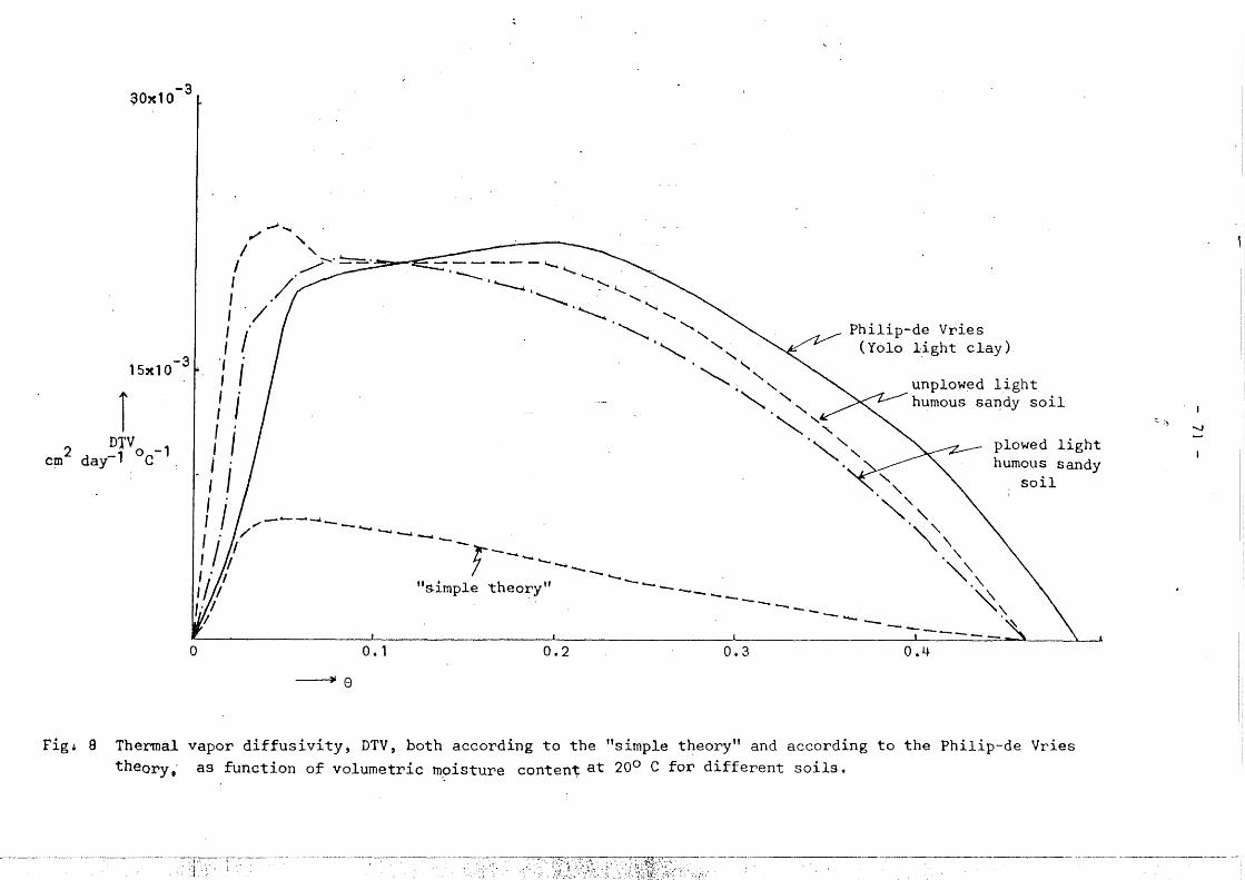
90x10-3
15x10-3
i 2 DTV
em day-1 °c-1.
~, --~, ,; ' --- .......... ' '--· ·- . ...._ I -·-- ~ . ..._, . ......,
I ./ ............... ........__ ',,
Philip-de Vries (Yolo light clay)
' / ...................... ', I·/ . ·~ ',, ' . ., ' 'I "" ' I - .""-- ", } i '""' ', I . I I I . I I J .
unplowed light humous sa~dy soil
plowed light humous sandy
soil I I
I,. ~-~-- .......... ___ _ I
~- r--~~~~-~ 1
"
I . ~heory ' r "S.l.mple
I . I
1/1 / ------------
1
. -._- ------I. I ''I
0 0., 0.2 0.3 0.4
----Ji 8
Fig• 9 Thermal vapor diffusivity, DTV, both according to the "simple theory" and according to the Philip-de Vries theory; as function of volumetric m~:>isture content at 20° C for different soils.
·.;
~~
"
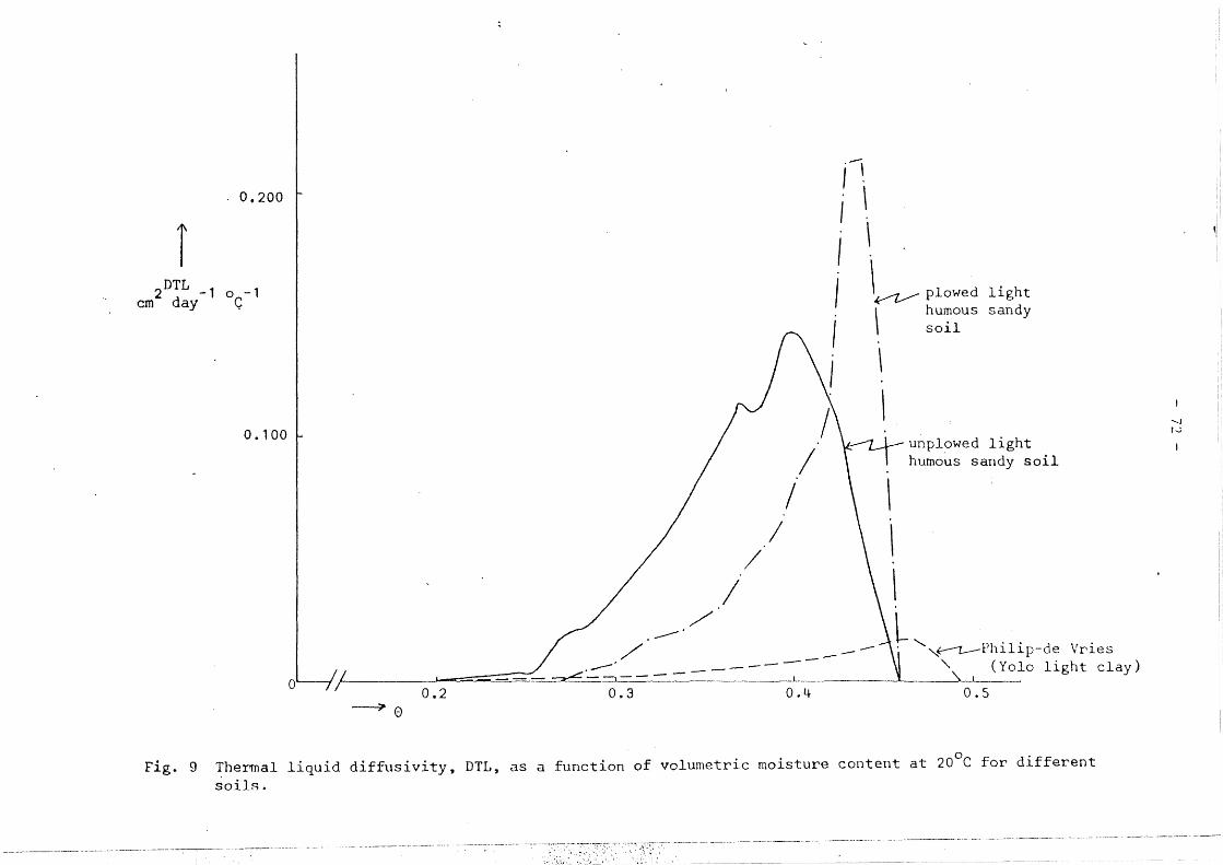
. 0. 200
i 2DTL -1 o -1
em day G
0.100
I /
---·
/
I I
I
j~. . \ I .
I I
I I ~plowed light sandy
I
I \ I
\ hu~ous so~l
\
\
I I I
unplowed light humous sandy soil
L, 'l ·1· · . / ~ '-__,_____,, 11 lp-de Vr1es
1 ~- --~· ~ ----~- "-\ , (Yolo light clay) I
/
0.2 0.3 0.4 0.5 ----;- 0
Fig .. 9 Thermal liquid diffusivity, DTL, as a function of volumetric moisture content at 20°C for different soils.
-......! r..;

o. 20
-r 2 DIF!1 0
... 1 em day C
0.100
0
unplowed ligh humous sandy soil
~ (l I \ I I I I
plowed light 1 '
humous ~ ~ sandy soil 1 ~
I ' ' \ I I I I I I I I
I ~ ' ' ' ' ' I ' I ' \
,. I // I
/ I
~/ ' /~ I
,..."' Ph. . 1 ~ ~~~ lllp-de Vries 1
~ ·· --- -= ---------"_,._---=:::..:::::.:::._ ____ L (Yolo light cla J -----I I
0. 1 0.2 0 .. 3 0.4 -------) 9
Fig. 10 Thermal moisture diffusivity, DIFT (~DTV + DTL), as a function of volumetric moisture content ·at 20°C for different soils.
""' l 0.5
""-..! w
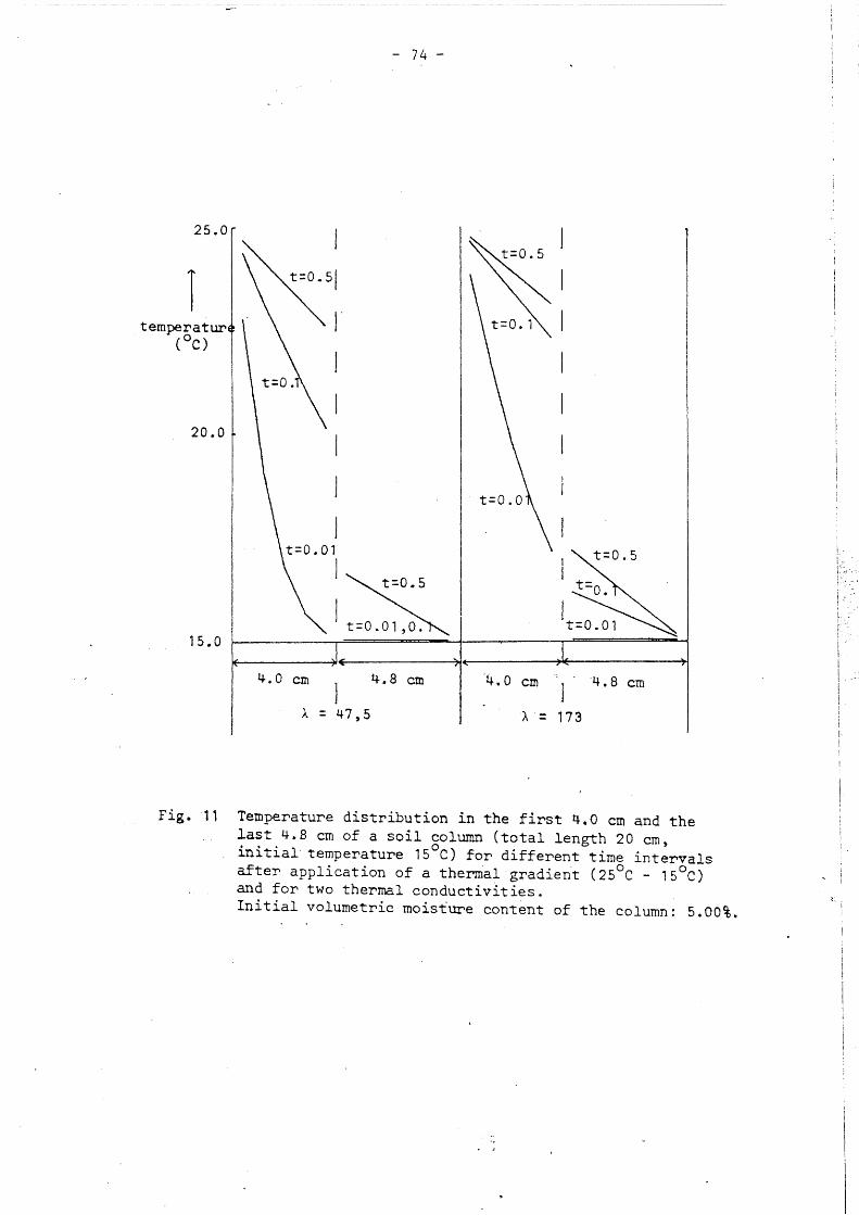
25.0
1
20.0
t=0.01
l
l 15.0
4.. 0 em
). = 47,5
- 74 -
4 .. 8 em
- j
~I
4.0 em
J
I
I
I t=o. .
It~
A = 173
Fig. ·11 Temperature distribution in the first 4.0 em and the last 4.8 em of a soil column (total length 20 em, initial temperature 15°C) for different time intervals after application of a thermal gradien·t (25°C - 15°C) and for two thermal conductivlties. Initial volumetric moisture content of the column: 5.00%.

8.6 em
i 23.
temperature · (°C)'
fig. 12
18,
13. I
Temperature distribution in soil column, 001 day (curve a, b and c) and 0.50 day (curved) after a sudden drop from 23°C to 13°C at one side. Curve a, b and c: initial volumetric moisture content of 4.5%, 9.0%, and 16.0%, respectively. Curve d: 4.5%, 9.0%, and 16.0% initial volumetric moisture.
·~'.1'.
'-I \J1
~
ll

8.6 em
r change
in % volumetric
0.60
0.40
moisture (absolute) · +0. 20
"" '· "", '' ........ "-... . "'. "---....._
\ ' '-.... I ·, ........... ....._
I '- -.....-..... I '-, ""'-...._-...........:
\ ' ---' ...... ----9i I( 13oc~·,, ...__ -J'~ ----- '----:-______ --~·-·
'} t= 0.10 t= 0.01 -0.20
0.40
0.60
(23°C)
---·-·-·-·-·-·--·-·-, __ _ -- ·-- . --..........:::-- ----. --------
Fig. 13 Moisture distribution in soil column after a sudden temperature drop from 23°C to 13°C at one side for different time intervals. Initial volumetric moisture content = 4.50%.
t=3.00
'-J 0'
~. - --~------·----------
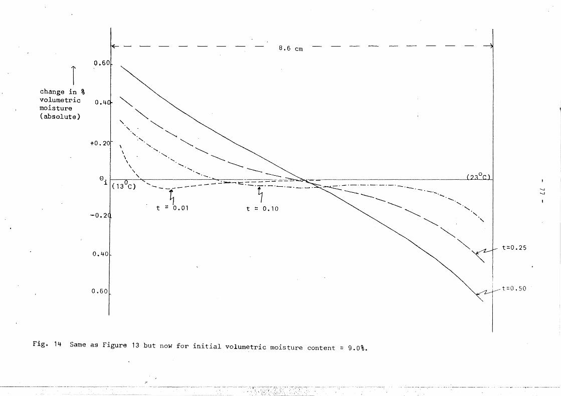
I change in % volumetric o. 4 moisture (absolute)
+0.20
""'""' ' ' ' \
' ·, ·.,
\ \
'""---~ ' ' "' '
~~
' " ' '
8.6 em
.........._ ____
' ·-. e . I ., .... _ . - :::. - - -1 ,._o_. ,_ ~---~- ~ --·t·-·-·-·-·-· ------
--~- I t = 0.01 t = 0.10
-0.2
0.40
0.60
·-·-·-·-·-·-·-·--........... ---·- ........ ::--::::.:.. ----- --- '
................. '· ~ '
"-..~
""'
Fig. 14 Same as Figure 13 but now for initial volumetric moisture content = 9.0%.
;•
t=0.25
t=O.SO
'-.1 '-.1
--..-- ---~---,..--- ......,..--.-------~--

I change in.% volumetric moisture (absolute)
___, -·- 8,6 em
0 .. 60
0.40
"· +o. 20
\ \
' "
\ \
'\
ei I( 13o0 ).
0.6
" ........ " ---....
' ........ -... (23°C)
--- :::::::.:-:·_--: ___ ·-·-·-. -:-·- ·- ............. ~ '· ---- -·-· . . ' ~--·-·-t~· ---- '
-- 7 . ~ ' ---1-~~- t~O.lO '-...._~" ',
t=O.Ol ""'
\
Fig. 15 Same as Figure 13 but now for initial.volurnetric moisture content = 16.0%.
-----~--- -·~---- ---·- -------------------~,------- ------- - -------------- -
t=0.25
t=O.SO
-.1
0:
i .;

1,·
o .60 I< ~ 8.6.cm
I I ' 0.40 change in % volumetric moisture (absolute) 0 •·20
r ..... ........ :-.. ........... ~ ...............
' ......... ' ' ........ ' .............. '-.....
0i I (13°C)
.......... . ............ """'- ..... .... . "" ..... ..... "" ..... ...
-0.20
0.40
0.60
', ·.......;::: ' . ', ..........._
', " ' ' ', "
', " ', ' ' ' ' ' ' ' ' \
\
(23°C)
"
e.=o'.o4s l.
0.=0.09 l.
\ I// 8. =0 • 16 \ A _), 1
\
' \
Fig. 16 Moisture distribution in soil column 0.5 day after a sudden temperature drop from 23°C to 13°C at one side for different initial volumetric molsture contents.~
i i·
-.....}
~

8.6 em ~ --
r a.o
change in % volumetric moisture (absolute)
6.0
Fig. 17
4.0
+ 2.0 b
e. (23°C) 1
-
2.0
4.0
Moisture distribution in soil column (total length 8.6 em), 1.0 day (curve a, band c) and 0.5 day (curve d) after a sudden temperature drop from 23°C to 13°C at one side. Curve a, band c: experimental data from Oomen and Staring (1972) for initial volumetric moisture contents of 5.10%, 9.05% and 15.75%, respectively. Curve d: simulation for an initial volumetric moisture content of 4.50 %.
co 0

25.
l temperature
0 ( C) 20.0
10.0
.......
' ' \ ' \
'\ \
\ '\
' ' ' ' ,// -=::::>""
constant I temperature at aol umn end j
t( FUDGE:;,] • )
/ ',~ --.._ I ......._
I / I /
I I I I
I I I I
11 II I
\ \ \
\ \
\ \
\ \
\ ., \
' ' ' -
I I
I
I volumetric
moisture content
isolated column (%)
I
I /
I
\FUDGE=~. )
..... ' / '
/ ' I
I
12.50
1 2. 00
s.o 0.5 --------------------------~~11.50 0
----) 1 • 0
time (days)
Fig. 18 Temperature (-) and moisture content (---) variation generated in the first compartment (0.8 em) of a horizontal soil column (total length 20 em) by a sinusoidal variation at the left side of the column. Initial temperature and volumetric moisture content: 15°C and 12%. Sinusoidal variation: average temperature 15°C
amplitude 10°C period 0.5 day
C0

rs.o temperature
(oC)
20.0
15.0
10.0
______ ..... _ .... - ---.. __
runGE=o. I ~~ and
---- .l_ FUDGE~l_:_ _I -- __. - - --... --
., volumetric
moisture content
(%)
---
5. 0 .J_ -----·----------
0 0.5 -----4 1 • 0
time (days)
Fig. 19 Same as Figure 18 but now for the second compartment of the soil ~olumn.
-----~-------- -----------·--
12.50
12.00
11 • 50
co !·.J

25.0
r tem~rature
(oC)
20.0
.l
I I I
~,,J . FUD~ 15.ol ~ ..---F 1 ~._-- =- ~ - I . l. _, -------------' ..._ ............... __._ -...,c.-
10.0
r volumetric
moisture content
(%)
s.o ~ 0 ~
0.5 , • 0
time (days)
Fig. 20 Same as Figure 18 but now for the last (25th) compartment of the soil column.
12.50
12.00 I
\ ~ 'I ,
:.
11 • 50

+1 i change in ° moisture percentage (%)
-1
+1
-1
-2
- 84 -
(14.5%)
6 7 -:..:.-::-----....... ~ c
- ---=--::._-~--=-- -a b
(7.8%)
----7 distance from heat source (em)
Fig. 21 The change in moisture percentage in respect to distance from the heat source after two cycles (of the applied heat wave), for two initial moisture contents (%by weight). a: period heat wave 8 min. b: Jt n If 16 min. c: 1f " n 32 min. (data from Hadas, 1968).


