Thixotropic gravity currents - University of British …njb/Research/thixo.pdfUnder consideration for publication in J. Fluid Mech. 1 Thixotropic gravity currents DUNCAN R. HEWITT1

Under consideration for publication in J. Fluid Mech. 1

Thixotropic gravity currents

D U N C A N R. H E W I T T1 †AND N E I L J. B A L M F O R T H2

1Department of Applied Mathematics and Theoretical Physics, University of Cambridge,Wilberforce Road, Cambridge, CB3 0WA, UK.

2Department of Mathematics, University of British Columbia, Vancouver, B.C. V6T 1Z2,Canada.

(Received ?; revised ?; accepted ?. - To be entered by editorial office)

We present a model for thixotropic gravity currents flowing down an inclined plane thatcombines lubrication theory for shallow flow with a rheological constitutive law describingthe degree of microscopic structure. The model is solved numerically for a finite volumeof fluid in both two and three dimensions. The results illustrate the importance of thedegree of initial ageing and the spatio-temporal variations of the microstructure duringflow. The fluid does not flow unless the plane is inclined beyond a critical angle thatdepends on the ageing time. Above that critical angle and for relatively long ageing times,the fluid dramatically avalanches downslope, with the current becoming characterised bya structured horseshoe-shaped remnant of fluid at the back and a raised nose at theadvancing front. The flow is prone to a weak interfacial instability that occurs along theborder between structured and de-structured fluid. Experiments with bentonite clay showbroadly similar phenomenological behaviour to that predicted by the model. Differencesbetween the experiments and the model are discussed.

Key words: Complex fluids, thixotropy, gravity currents.

1. Introduction

Thixotropic fluids have a time-dependent microstructure that gradually builds up whenthe fluid is at rest, leading to a slow increase in the effective viscosity, but is reversiblybroken down by flow, thereby lowering the fluid’s resistance (Mewis & Wagner 2009).A wide range of fluids exhibit thixotropic behaviour, including natural clay suspensions,industrial drilling fluids and cements, printing inks and paints, oils and grease, and foodproducts such as mayonnaise and ketchup (Barnes 1997; Mewis & Wagner 2009). Akey feature of these thixotropic fluids is that they may experience so-called “viscositybifurcations” (Coussot et al. 2002a; Bonn et al. 2004; Moller et al. 2009; Alexandrou et al.2009): if the fluid is jammed in a structured or solid state with high viscosity, an increasein the stress on the material beyond a critical threshold can cause the microstructureto abruptly disintegrate, substantially lowering the viscosity and initiating sudden fluidflow. Moreover, if the stress is reduced below another (typically lower) critical value,the microstructure can swiftly recover and jam, abruptly increasing the viscosity andblocking flow.

Gravity currents form a particularly important class of flows in which viscosity bi-furcations can play a significant role. Many geophysical muds and clays appear to bethixotropic, and the relatively sudden and long runouts of mudslides and “quick-clay”

† Email address for correspondence: [email protected]

2 D. R. Hewitt, N. J. Balmforth

avalanches has been suggested to originate from this rheology (Khaldoun et al. 2009). Inindustrial settings, currents of mine tailings and waste mineral slurries have been observedto flow much further than predicted (Henriquez & Simms 2009; Simms et al. 2011), withpotentially serious environmental consequences. On a different scale, household food-stuffs such as ketchup are often tested in the “Bostwick consistometer” (a variant of theclassical dambreak problem in which material is suddenly released and slumps down achannel; Balmforth et al. 2006a), yet the confounding role that thixotropy can play insuch a device is usually ignored.

Key features of thixotropic gravity currents were documented in the experiments ofCoussot et al. (2002a). These authors observed that a suspension of bentonite clay em-placed as a mound on an inclined plane did not flow provided the slope was belowa certain critical angle. Above that angle, however, the mound collapsed dramatically,with a fraction of the clay flowing rapidly down the incline, and a horseshoe-shapedremnant of immobile material being left behind. The critical angle corresponds to thestress at which a viscosity bifurcation occurs; the avalanching fluid having de-structuredand separated from the structured horseshoe-shaped remnant. For uniform layers on aninclined plane, Huynh et al. (2005) showed that the critical angle increased if the fluidwas left to rest and “age” for longer. Similar “avalanche” behaviour was recorded for claysuspensions by Khaldoun et al. (2009); these authors also reported that the collapse wasmediated by a thin de-structured basal layer, upon which the overlying rigid bulk of thematerial was conveyed.

Although previous work has proposed constitutive laws describing the viscosity bi-furcations of thixotropic fluid (see §2), there have been few attempts to couple suchrheological models with the detailed flow dynamics. In particular, there has been noattempt to model the spatio-temporal evolution of a thixotropic gravity current on aninclined plane. Our aim in the current paper is to provide such a model. In particular,we present a detailed shallow-layer theory that describes the release of a finite volume ofthixotropic fluid on a slope. Such theories are well documented for Newtonian (Huppert1982; Lister 1992) and viscoplastic (Liu & Mei 1989; Balmforth et al. 2002, 2006b) fluids.

Our rheological model, a simple thixotropic constitutive law incorporating viscositybifurcations, is described in §2. In §3, we couple this rheology with lubrication theoryfor shallow flow. We solve the equations of the model numerically in section §4, in bothtwo and three dimensions, and discuss the main features of the flow. In §5, we presentexperimental results for gravity current of an aqueous suspension of bentonite clay. Thereis broad agreement between the theory and experiments, but there are also some notabledifferences, which are discussed here. Finally, in §6 we summarize our main results.In exploring the theoretical model, we encounter a novel type of interfacial instability;additional details of this feature of the model are presented in the Appendix.

2. Rheological model

2.1. Background

Viscosity bifurcations can be rationalized using simple constitutive models that exploita parameter, λ(t), which describes the degree of internal structure (Barnes 1997; Mewis& Wagner 2009). Here, we take this parameter to lie in the range [0, λ0 ]: the fluid has noeffective microstructure if λ = 0, but is fully structured and solid-like when λ = λ

06 1.

The structure parameter controls the viscosity µ(λ) in the generalized Newtonian fluidmodel,

τij = µ(λ) γij , (2.1)

Thixotropic gravity currents 3

which relates the deviatoric stress tensor τij to the rate of strain tensor γij . The structureparameter is often taken to satisfy an evolution equation of the form,

dλ

dt= g(λ, γ) = G(λ, τ), (2.2)

where γ =√γij γij/2 and τ =

√τijτij/2 denote tensor invariants, and G(λ, τ) follows

from g(λ, γ) on using (2.1). Various forms for µ(λ) and g(λ, γ) have been proposedin the literature (Coussot et al. 2002a,b; Moller et al. 2006; Dullaert & Mewis 2006;Putz & Burghelea 2009; Alexandrou et al. 2009). In general, g(λ, γ) contains a positiveterm corresponding to restructuring or “healing”, and a negative term proportional to γdescribing the de-structuring effects of flow. The viscosity µ(λ) increases with structure,and becomes large or even diverges as the fluid becomes fully structured.

The viscosity bifurcations occurring as stress is varied are conveniently illustrated usingthe quasi-steady version of (2.2), G(λ, τ) = 0. The overall idea is that, for low or vanishingstress, G(λ, τ) is a positive, decreasing function of λ that vanishes only for λ = λ0 ;see figure 1(a). As is clear from (2.2), G(λ0 , τ) = 0 corresponds to a fully structuredequilibrium state that is stable when ∂G(λ

0, τ)/∂λ < 0. As the stress is increased, the

curve representing G(λ, τ) is pushed down somewhere over the range of λ, eventuallytouching the G(λ, τ) = 0 axis and creating two new equilibrium states, λ = λ±, at acritical stress, τ = τ

C. The newly created state with less structure, λ = λ− < λ+, is

stable, whilst that with an intermediate degree of structure, λ = λ+, is unstable. Thefully structured state λ = λ0 persists during the bifurcation, however, and remains stable,implying that the fluid would remain in this state if it was prepared so before the stresswas increased.

A second viscosity bifurcation arises if the stress is increased still further: the curveof G(λ, τ) continues to be driven downwards, and the unstable equilibrium moves tohigher λ. Eventually, this state collides with the fully structured solution at λ = λ

0,

rendering that equilibrium unstable (∂G(λ0, τ)/∂λ becomes positive). This bifurcation

occurs at stress τ = τA

; for higher stresses τ > τA

, the only stable equilibrium in therange [0, λ0 ] is λ = λ−. Therefore, all structure disintegrates and evolves towards the de-structured equilibrium, even if the fluid were initially fully structured. The set of curveswith increasing stress in figure 1(a) illustrate a sequence of such situations.

The behaviour of the structure function in figure 1(a) implies a hysteretic relationbetween stress τ and strain rate γ if the stress on a sample of fluid is first ramped upuntil flow occurs, and then decreased back down until the flow subsides. More specifically,as sketched in figure 1(b), the fluid is initially static and fully structured (λ = λ

0and

γ = 0), and remains so until that state loses its stability at τ = τA

. The fluid structurethen disintegrates and evolves towards the less structured state λ = λ− with finite shearrate. If the stress is then lowered, the flowing, less structured state of the fluid is preserveduntil τ falls below τ

C, at which juncture that state disappears. Thereafter, the flow can

no longer destroy the microstructure at the same pace as it heals, and the fluid evolvesback towards the structured state, with the viscosity abruptly increasing and the flowcoming to a halt.

2.2. The rheological model

Our aim is to present a simple model of thixotropic gravity currents. For the task, weincorporate the thixotropic rheology, and specifically the viscosity bifurcations, in assimple a manner as possible. More precisely, we use the structure function shown infigure 1(a) to relate the local stress to the microstructural state. That is, given thestress, we solve G(λ, τ) = 0 to determine λ, and thence the viscosity, µ(λ).


! !"# !"$ !"% !"& '!!"#

!

!"#

!"$

!"%

!"&

()*

!"

!"+ !"& !", '

!!"!#

!!"!'

!

!"!' λ0= 1/2

λ0= 1

τ = τA

τ = τC

G(λ, τ)

λ/λ0

γ

τ

!"#$

!"#%

!""

!"%

!"

%"

&"

$"

'"

(Pa)

(s−1)

τ

γ

!!"!""

τC

τA

τC

τA

Figure 1: (a) The structure function G(λ, τ) for four values of the stress τ . The curvesare based on the model (2.4). The dashed and dot-dashed curves show the critical casesτ = τ

Cand τ = τ

A. Stars indicate the stable, less structured equilibrium states, and

circles indicate the unstable, intermediate structured states. Panel (b) shows a sketch ofthe hysteretic stress-strain-rate relation, with the arrows indicating the pathway expectedfor an experiment in which stress is first increased past the critical value τ

A, and then

decreased back below τC

. The dashed line shows the unstable, intermediate structuredequilibrium. The light dotted lines show the stress-strain-rate relations for λ

0= 1/2

(idealized yield-stress-like behaviour) and λ0

= 1 (τA→∞). The inset shows rheometric

data for a bentonite clay suspension (7.5wt% ≈ 10% by volume) in a cone and platerheometer. The stress was increased from 10 Pa to 50 Pa in 20 steps, and then decreasedagain, waiting for 5 seconds at each stress level. The fluid was pre-sheared for 2 minutesat 100 Pa, and left to rest for 5 minutes before starting the test.

A convenient form for the structure function is furnished by the models,

g(λ, γ) =(λ0 − λ)

λ0T− αλγ and µ(λ) =

µ0λ0

(1− λ) (λ0− λ)

, (2.3a, b)

which imply

G(λ, τ) =(λ

0− λ)

λ0T[1− Γλ (1− λ) τ ] = 0, (2.4)

where T and α are positive empirical constants, µ0 is a constant reference viscosity andΓ = αT/µ0. The two terms on the right-hand side of (2.3a) can be interpreted as thehealing of the microstructure and flow-induced de-structuring, respectively.

The forms in (2.3) are similar, but not identical, to those suggested by Barnes (1997),and many authors since. The main differences are the factor (λ

0− λ)(1 − λ) in µ(λ)

(2.3b) rather than a power of (1− λ), and our identification of the fully structured stateas λ = λ0 , not λ = 1 or λ = ∞. These differences are key to ensuring that there is asecond viscosity bifurcation at τ = τ

Aas discussed above, and to accommodate differing

degrees of initial ageing (see §2.3 below). In any event, (2.4) is an especially convenientfrom of the structure function, because it can be solved analytically to give the three


branches of the stress-strain-rate relation:

λ = λ0, λ = λ±(τ) =

1

2

[1±

(1− 4

Γτ

)1/2]. (2.5a, b)

The points of bifurcation can also be determined analytically: the stable-unstable pair ofequilibria, λ = λ±, appear for τ > τ

C= 4/Γ; and the fully structured state is unstable

for τ > τA

= [Γλ0(1− λ

0)]−1.

Over the range τC< τ < τ

A, the stress-strain-rate relation has three possible solutions,

raising the question of how to select the appropriate structural state given the stress. Wedismiss the choice λ = λ+, as this state corresponds to an unstable equilibrium. Theselection between the other two options, λ = λ− and λ = λ

0is dictated by the stress

history of the fluid: if the material has never been subjected to a stress exceeding τA

,then the fluid structure has never disintegrated, and λ = λ

0. On the other hand, if the

structure did disintegrate at some moment in the past (with τ > τA

), then the fluid is inits less structured state, and λ = λ−.

Note that our use of G(λ, τ) in this fashion corresponds to assuming that the disinte-gration of the microstructure for τ > τ

A, or restructuring for τ 6 τ

C, is instantaneous

(as in a kind of rapid phase transition). The differential constitutive law in (2.2) allowsfor a more general version of the scenario, and in particular for delays in disintegrationor restructuring. Hence, our model can be thought of as the quasi-steady version of (2.2).However, retaining the time rate of change of λ in the rheological model complicatesthe theory significantly. On the other hand, constitutive laws are often little more thanmathematical formulations of flow-curve cartoons based on a combination of physical in-tuition and rheometric data. Hence, it is not clear that (2.2) conveys much more physicalrealism that the statement G(λ, τ) = 0. Indeed, when supplemented with the rules forselecting amongst the multiple branches of the stress-strain-rate relation, (2.4) can beviewed as a constitutive law in its own right.

2.3. Ageing

Rheological measurements (see e.g. Moller et al. 2009) suggest that the critical thresholdfor flow to begin, τ

A, depends on the ageing time of the fluid Tage. This timescale can be

of the order of several minutes or even hours, and is typically longer than the durationof a gravity current flowing down an incline in a laboratory experiment. We thereforemake the assumption that, although ageing controls the threshold for initiation of flow,it takes place too slowly to influence the dynamics of the gravity current.

We incorporate the effect of ageing into our model via the parameter λ0 . More precisely,as shown in figure 1(b), when λ0 → 1

2 , the hysteresis loop of the stress-strain-rate rela-tion disappears, leaving a single-valued curve representing the stable equilibrium. Thisstate is fully structured for τ < τ

C= τ

A= 4/Γ, but de-structures and flows at higher

stresses. That is, structure formation and disintegration take place at a common criticalor yield value; the behaviour is equivalent to that of an idealized yield-stress fluid (witha nonlinear viscosity). If the fluid were not left to age at all, this would correspond tothe observed situation. As λ0 → 1, on the other hand, the threshold τ

Adiverges, which

indicates (somewhat unphysically) that the fluid never de-structures. This situation issuggestive of an arbitrarily long period of ageing. Thus, taking different values for λ

0

between these two limits allows for differing degree of initial ageing: the bigger the valueof λ

0, the longer the ageing time Tage.


θ

θ

x

z

L

H

y

z = h z = h

z = Yz = Y

z = zA

z = zC

z = zA

z = zC

Figure 2: A sketch of the flow geometry, showing the coordinate system, the characteristiclength and depth, L and H, the local fluid depth h(x, y, t), and the curves of the constantcritical shear stresses, z

A= z(τ

A) and z

C= z(τ

C). The border between structured and

destructured fluid, z = Z(x, y, t), is pieced together from z = zA

, zC

and a materialsection, z = Y (x, y, t); destructured fluid is shown shaded. The left-hand plot shows theprofile in z of u through a slice of the flow.

3. Shallow flow model

3.1. Dimensional formulation

As sketched in figure 2, we consider flow over an inclined plane with velocity u = (u, v, w)described by a Cartesian coordinate system (x, y, z), orientated such that the x-axispoints downslope and the y-axis points across the slope. The plane is inclined at anangle θ. The fluid is shallow, with a characteristic depth H that is much smaller thanthe characteristic lengthscale for variations over the plane, L, so that the aspect ratio isε = H/L� 1. The local fluid depth is z = h(x, y, t).

The flow is incompressible,

∂u

∂x+∂v

∂y+∂w

∂z= 0, (3.1)

and satisfies the momentum equations,

ρ

(∂u

∂t+ u · ∇u

)= ρg −∇p+∇ · τ , (3.2)

where p is the pressure, and g = (g sin θ, 0,−g cos θ), with constant gravitational ac-celeration g. The deviatoric stresses are related to the rate of strains by (2.1), and theviscosity is set according to (2.3) and (2.4). Just prior to the moment that the fluid isreleased, the material is fully and uniformly structured, so that λ = λ

0.

The boundary conditions are given by no slip at the base and the stress-free conditionat the upper boundary:

u = 0 at z = 0, (τij − pδij)nj = 0 at z = h(x, y, t), (3.3a, b)

where n is the normal to the surface z = h. The kinematic condition at the upperboundary is

∂h

∂t+ u

∂h

∂x+ v

∂h

∂y− w = 0 at z = h(x, y, t). (3.4)


3.2. Dimensionless leading-order formulation

To remove the dimensions from the equations and pave the way for the shallow-layertheory, we introduce the rescalings,

t =L

Ut∗, (x, y) = L(x∗, y∗), (z, h) = H(z∗, h∗), (3.5)

(u, v) = U(u∗, v∗), w = εUw∗, p = ρgHp∗ cos θ, τij =µ0U

Hτ∗ij , (3.6)

µ = µ0µ∗, G = TG∗, Γ =

αTU

HΓ∗, (3.7)

where the speed scale

U =H3ρg

Lµ0cos θ.

On discarding the star decoration, and to leading order in ε, (3.2) reduces to the lubri-cation equations

0 = S − ∂p

∂x+∂τxz∂z

= −∂p∂y

+∂τyz∂z

= −1− ∂p

∂z, (3.8)

where the slope parameter S = ε−1 tan θ is assumed to be O(1). The neglect of inertialterms is valid provided that the Reynolds number Re = ρUL/µ0 is no larger than O(ε−1).The dimensionless viscosity and structure function can be written as

µ =λ

0

(λ0− λ)(1− λ)

, G =(λ

0− λ)

λ0

[1− Γτλ(1− λ)] = 0. (3.9a, b)

The dominant components of the rate of strain tensor are γxz = ∂u/∂z + O(ε2) andγyz = ∂v/∂z+O(ε2). Therefore, to leading order, the stress conditions in (3.3b) become

p = γxz = γyz = 0 at z = h(x, y, t). (3.10)

The kinematic condition (3.4) is unchanged after scaling.Equations (3.8) and (3.10) imply that the pressure is hydrostatic,

p = h− z, (3.11)

and the shear stresses are given by (τxz, τyz) = (h − z)(S − ∂h/∂x,−∂h/∂y), so τ =√τ2xz + τ2yz = (h− z)T , with T =

√(S − ∂h/∂x)2 + (∂h/∂y)2.

3.3. Anatomy of the flow

The rheological model in (3.9) implies that changes in fluid structure occur when thelocal stress invariant τ ≡ (h−z)T becomes equal to one of the critical values, τ

Cand τ

A.

The stress contours τ = τC

and τ = τA

therefore define two surfaces, z = zC

= h− τC/T

and z = zA

= h − τA/T . Above z = z

C, the stress is less than τ

C, indicating that

the fluid is structured with λ = λ0 and γ = 0. That is, the flow is plug-like with∂u/∂z = ∂v/∂z = 0. On the other hand, below z = zA, the stress is greater than τ

A, and

the fluid is de-structured with λ = λ−, indicating that there is vertical shear, γ > 0.Between the two stress surfaces, z

C< z < z

A, the structural state of the fluid depends

on the stress history of each fluid element. Initially, the fluid is prepared in the fullystructured state with λ = λ

0everywhere. Therefore, when the fluid is released, the de-

structured fluid will be exactly bounded above by z = zA

. During the ensuing flow, ifthe stress increases locally this surface may migrate upwards into structured fluid and


de-structure that material. However, the runout of the fluid can also reduce the localstress, demanding that the surface z = z

Adescend through the fluid, leaving behind

de-structured fluid. Those fluid elements move with the flow and only de-structure whenthe local stress falls below τ

Calong the level z = z

C.

Thus, the interface, or yield surface, z = Z(x, y, t) which separates de-structured fluidfrom fully structured fluid, must consist of three different segments. First, there is ade-structuring front Z ≡ zA wherever the surface z = z

Ais ascending into currently

structured fluid. Second, there is a re-structuring front Z ≡ zC

whenever the surfacez = z

Cis descending into currently de-structured fluid. Third, in between these fronts

there is a yield surface corresponding to the border of material that was initially de-structured by an increase in local stress, but was then left behind as stresses declined;this piece of the yield surface is necessarily a material curve, Z ≡ Y (x, y, t), which satisfiesthe kinematic condition,

∂Y

∂t+ u

∂Y

∂x+ v

∂Y

∂y− w = 0 on z = Y (x, y, t). (3.12)

The yield surface and its constituent pieces are illustrated in figure 2.

3.4. Synopsis of the model

In summary, the spreading velocity of our thixotropic current is determined by integrat-ing

µ∂u

∂z=

(S − ∂h

∂x

)(h− z) ≡ τxz and µ

∂v

∂z= −∂h

∂y(h− z) ≡ τyz, (3.13a, b)

where

µ(λ) =λ

0

(1− λ) (λ0− λ)

, (λ0− λ) [1− Γτλ (1− λ)] = 0, (3.14a, b)

and

τ =√τ2xz + τ2yz = T (h− z) , T =

√(S − ∂h

∂x

)2

+

(∂h

∂y

)2

. (3.15a, b)

The relevant root 0 6 λ 6 λ0 of (3.14b) is given by the local stress history, as discussedin §2.2 and §3.3. The local fluid depth evolves according to (3.4), or, using the integralof (3.1),

∂h

∂t+

∂

∂x

∫ Y

0

(h− z) ∂u∂z

dz +∂

∂y

∫ Y

0

(h− z) ∂v∂z

dz = 0. (3.16)

The yield surface z = Z(x, y, t) follows z = zA

= h − τA/T if that curve is moving up

into structured fluid, or matches z = zC

= h− τC/T if this surface is moving down into

de-structured fluid. Otherwise, the yield surface evolves as a material curve as in (3.12);equivalently,

∂Y

∂t+

∂

∂x

∫ Y

0

(Y − z) ∂u∂z

dz +∂

∂y

∫ Y

0

(Y − z) ∂v∂z

dz = 0. (3.17)

We solve equations (3.16)-(3.17) numerically, in both two and three dimensions, usingsecond-order centred finite differences in space, and a second-order midpoint method intime. We place a thin pre-wetting fluid film (of thickness h = 10−3) on the substrateto avoid any difficulties with a moving contact line. The flux terms in (3.16) and (3.17)can be evaluated analytically to expedite the computations (the expressions for theseintegrals are rather convoluted and not very informative, so we avoid quoting them).


!!"# !! !$"# !$ !%"# % %"# $ $"# ! !"#%

%"$

%"!

%"&

%"'

%"#

%"(

%")

%"*

%"+

$

!!"# !! !$"# !$ !%"# % %"# $ $"# ! !"#%

%"$

%"!

%"&

%"'

%"#

%"(

%")

%"*

%"+

$ 0 0.2 0.4 0.6 0.8 1 1.2 1.4 1.6 1.8 20

0.1

0.2

0.3

0.4

0.5

0.6

0.7

0.8

0.9

1

0 0.2 0.4 0.6 0.8 1 1.2 1.4 1.6 1.8 20

0.1

0.2

0.3

0.4

0.5

0.6

0.7

0.8

0.9

1

0 0.4 0.8 1.2 1.6 2-2 -1 0 1 20

1

0.8

0.6

0.4

0.2

0

1

0.8

0.6

0.4

0.2

(a)

(c)

(b)

(d)

xx

z

z

Figure 3: Planar slumps on a horizontal plane (S = 0) for (a-b) λ0

= 0.8 and (c-d)λ0 = 0.95, with Γ = 40 (τ

C= 0.1). Panels (a) and (c) show snapshots of the free surface

z = h at times t = 0, 1, 2, 4, 8, 16, 32, and 64, together with the final rest state (dashed)from (4.2). Panels (b) and (d) show z = h (solid blue), z = z

C(dashed), and z = z

A

(dotted) in x > 0 at t = 20; de-structured fluid is shown shaded. In (b), the materialpart of the yield surface z = Y is very short, and Z = z

Cover most of the fluid. In (d),

z = zA

is positive only very close to the moving front.

The characteristic length scales of the flow L and H can be used to scale out two ofthe free parameters of the problem. For all the results presented here, we fix the totalvolume of fluid V = 2 and the initial height of the fluid h(t = 0) = 1. We are then leftwith three free parameters: the slope S, the structure parameter λ

0, and Γ, which sets

the critical stresses τC

and τA

.

4. Numerical results

4.1. Two-dimensional slumps on a horizontal plane

We begin by considering the planar slumping on a horizontal plane (S = 0) of a rectan-gular block of fluid with initial profile, h(x, 0) = 1 for −1 ≤ x ≤ 1 and h(x, 0) = 0 for|x| > 1. Figure 3 shows snapshots of numerical solutions for two values of λ0 , and Γ = 40.For the case with less initial structure (λ0 = 0.8; panels a-b), the fluid slumps much likean idealized yield-stress fluid (e.g. Balmforth et al. 2006b), and the yield surface z = Zlies mostly along the stress contour z = z

C. For greater initial stucture (λ

0= 0.95; pan-

els c-d), the nose of the current advances in a similar fashion to the lower value of λ0.

However, raised interior the flow collapses much more slowly because the fluid there onlyde-structures over a relatively thin basal region, the stress never having exceeded τ

Aover

most of the fluid.We define x

N(t) as the position of the right-hand nose of the current, and x

B(t) as

the location of the rear of the moving section of fluid in x > 0 (i.e. the least positivevalue of x at which h = 1; the “back” of the current). In view of the initial condition,x

N(0) = x

B(0) = 1, and all the fluid is in motion once x

Bdecreases to 0. Figure 4 plots

time series of xN

(t) and xB

(t) for the two solutions shown earlier in figure 3, along withother solutions for different values of Γ and ageing times. For small Γ, τ

Aand τ

Care

large and the fluid does not slump very far, coming to rest before xB

reaches the origin.With higher Γ, more fluid de-structures and the slump flows further. The degree of ageing


!"!#

!"!$

!""

!"$

"

!

$

%

0 0.5 1 1.5 2 2.5 3 3.5 40

0.5

1

1.5

λ0= 0.95λ

0= 0.9λ

0= 0.8λ

0= 0.7

t

xN

xB

xN

xB

t

Γ = 4

Γ = 40

Γ = 400

Γ = 4

Γ = 40Γ = 400

(a)

(b)

!! " !"

"#!

$

x

h

Γ = 4

Γ = 40Γ = 400

Figure 4: Time series of xN

(t) (solid) and xB

(t) (dashed) for planar slumps on a horizontalplane (S = 0). Panel (a) shows results for the values of Γ indicated, at fixed initialstructure λ0 = 0.8; the inset shows the final states given by (4.2) and (4.3). Panel (b)shows results for the values of λ0 indicated, at fixed Γ = 40.

(λ0) exerts little influence on the advance of the nose of the current because the stress isalways increased sufficiently to exceed τ

Aby steepening the slope there. However, x

B(t)

retreats increasingly slowly as λ0

increases, in agreement with the results in figure 3.In all cases, the slump finally comes to rest when all the material re-structures com-

pletely. This arises when the stress falls below τC

everywhere, which, from (3.13) withz = S = τyz = 0, demands that ∣∣∣∣h∂h∂x

∣∣∣∣ ≤ τC =4

Γ. (4.1)

If Γ < 12, the yield stress τC

is large enough that xB

never reaches x = 0, and a centralsection of fluid remains immobile with h = 1; elsewhere, the equality in (4.1) is attained.Hence,

h(x) =

{1 if |x| < X1,[

1− 8Γ−1 (|x| −X)]1/2

if |x| > X1;X1 = 1− 1

12Γ. (4.2)

If, instead, Γ > 12, then the fluid fully slumps, the equality in (4.1) applies throughoutand

h(x) =

[8

Γ(X2 − |x|)

]1/2; X2 =

(9Γ

32

)1/3

. (4.3)

The final states predicted by (4.2)-(4.3) are included in figures 3 and 4, and are identicalto those obtained for an idealized yield-stress fluid with yield stress τ

C(see e.g. Balmforth

et al. 2006a). Although the final slumped states do not depend on the initial structure λ0,

the numerical results in figure 4 emphasize how the approach to the final state becomesincreasingly long as λ

0increases towards 1.


!! " ! # $ % &""

"'!

"'#

"'$

!! " ! # $ % &""

"'!

"'#

"'$

!! " ! # $ % &""

"'!

"'#

"'$

!! " ! # $ % &""

"'!

"'#

"'$

!! " !"

"#!

"#$

"#%

!! " !"

"#!

"#$

"#%

!! " !"

"#!

"#$

"#%

!! " !"

"#!

"#$

"#%

(a)

(b)

(c)

(d)

(e)

(f)

t = 0

t = 0

t = 0

t = 0

t = 300

t = 300

t = 300

t = 300

x

x

x

z

z

z

z

z

z

!! " ! # $ % &" &! &# &$ &%"

"'!

"'#

"'$

!! " ! # $ % &" &! &# &$ &%"

"'!

"'#

"'$

Figure 5: Inclined planar slumps for S = 1 and Γ = 40 (τC

= 0.1). Shown are theheight z = h (solid blue), and the stress contours z = z

C(dashed) and z = z

A(dotted);

de-structured fluid is shown shaded. Panels (a)–(d) show profiles at t = 0 (left) andt = 300, for: (a) a Bingham fluid with yield stress τ

C= 0.1; (b) thixotropic fluid with

λ0

= 0.8; (c) λ0

= 0.9; (d) λ0

= 0.95. Initially, z(τA

) = Z, and at t = 300 in (c) and(d), z(τ

A) is mostly negative. Panels (e)–(f ) show snapshots of the height z = h at

t = 0, 10, 20, 40, 80, 160, 320 and 640, for (e) λ0 = 0.8, and (f ) λ0 = 0.95; the final states,given by (4.7), are shown by the dashed line.

The numerical solutions in figure 3 expose a crucial hidden detail of the theoreticalmodel. It is evident from the snapshots of h(x, t) that fluid spreads out from the midlineof the slumping current at x = 0. This spreading is mediated by the de-structured lowerlayer of the fluid, which conveys along the overlying structured fluid. Importantly, eventhough the structured fluid flow is plug-like in the vertical (∂u/∂z = 0), this material stillundergoes a much weaker horizontal extension. In other words, the structured fluid is notrigid, despite the infinite viscosity suggested by (3.9). This inconsistency is equivalentto the lubrication paradox of a yield-stress fluid (see Balmforth & Craster 1999) and isresolved as follows: the shallow-flow approximation of §3 amounts to the leading-orderof an asymptotic expansion. Implicitly, it assumes that the viscosity of the structuredfluid is sufficiently large that it suppresses the vertical shear. However, the viscosity isnot taken to be so large that the extensional stresses, τxx ≡ −τzz, become promoted


0 100 200

1.5

2

2.5

3

3.5

4

4.5

0 50 100 150 200 2502

4

6

8

0 50 100 150 200 2502

4

6

8 0.80.9

0.95

0.94

0.955

0.96

0.9620.95

0.80.9(a) (b)

xN

tt

0.96 0.968

0.7

xN

0.95

0.96

0.80.90.92

0.94

t

(c)

Figure 6: Position of the nose xN

(t) with Γ = 40, for the values of the initial structureλ0 indicated: (a) two-dimensional slump with S = 0.8; (b) two-dimensional slump withS = 1; (c) three-dimensional slump with S = 1. The dotted lines show the results for aBingham fluid with yield stress τ

C= 0.1. For the largest value of λ

0in each subfigure,

the slope is below the critical angle, and the current remains stationary.

into the leading-order balance of forces in (3.8). In other words, our structured fluid doesnot have an infinite viscosity, merely one that is large; in our asymptotic scheme, theunderlying assumption is that 1 � µ(λ0) � ε−1. Consequently, the enhanced viscosityof the structured fluid only suppresses the vertical shear, not the horizontal extension.We return to this important point later in §5.2.1.

4.2. Two-dimensional slumps on an inclined plane

4.2.1. Results

Motivated by our experiments in §5, we initiate planar, inclined slumps (S > 0) bytaking the initial height profile to be given by the final rest state of a slumped domeon a horizontal plane. That is, h(x, 0) is set by either (4.2) or (4.3), depending on thevalue of Γ. In order to avoid discontinuities in the stress, the initial profile is smoothed atpoints where the free surface has a discontinuous derivative (i.e. for Γ > 12, the heightis smoothed at x = 0). Figure 5 shows numerical results for three different ageing times,with Γ = 40 (τ

C= 4/Γ = 0.1) and S = 1. For comparison, panel (a) shows a solution for

a Bingham fluid (an idealized yield-stress fluid with a linear constitutive law) with thesame yield stress τ

C. The height profile of the Bingham current increases from the back,

where the fluid remains stationary, to a maximum just behind the front. The thixotropiccase with smaller ageing time (λ

0= 0.8; panels b, e) shows broadly similar features. For

longer ageing (λ0

= 0.9 and 0.95; panels c, d, f ), however, the current leaves behind astriking raised remnant of structured fluid, and develops a pronounced raised nose at thefront. These features result because the stress on the fluid is greatest below the highestpoint of the initial profile; the most significant de-structuring then occurs at the centreof the current.

Time series of the position of the nose of the current xN

(t) for a suite of computationsat fixed Γ = 40 are shown in figure 6. For small values of λ

0, the current travels faster

than the corresponding Bingham fluid because the de-structured thixotropic materialhas a smaller, rate-dependent viscosity. The currents of older fluid (larger λ0) are slower,however, and are characterized by an increasingly long delay at the beginning of thecomputation before the nose of the current starts to move. Moreover, if λ

0is too large,

the fluid never moves at all; this points to an age-dependent critical slope that must beexceeded in order for the fluid to collapse (compare the solutions for S = 0.8 and S = 1in figure 6a and b). The critical slope is discussed further in §4.2.2.


!!"# !! !$"# !$ !%"# % %"# $ $"# ! !"#%

%"$

%"!

%"&

%"'

%"#

%"(

%")

!!"# !! !$"# !$ !%"# % %"# $ $"# ! !"#%

%"$

%"!

%"&

%"'

%"#

%"(

%")!!"# !! !$"# !$ !%"# % %"# $ $"# ! !"#%

%"$

%"!

%"&

%"'

%"#

%"(

%")

!!"# !! !$"# !$ !%"# % %"# $ $"# ! !"#%

%"$

%"!

%"&

%"'

%"#

%"(

%")

-2 -1 0 1 2

0

0.2

0.4

0.6

0

0.2

0.4

0.6

(a) (b)

(c) (d)

t = 0 t = 1

t = 3 t = 7

-2 -1 0 1 2

z

z

xx

Figure 7: Four snapshots of the current in figure 5f (Γ = 40, S = 1, λ0 = 0.95), at thetimes indicated. Shown are the height z = h (solid blue) and the two stress contoursz = z

C(dashed), z = z

A(dotted); de-structured fluid is shaded.

The initial delay in the advance of the nose arises because, at angles just above thecritical value, the fluid only de-structures in the centre of the current. The dynamics isshown in more detail in figure 7, which displays the early-time evolution of the currentof figure 5f with λ

0= 0.95. At t = 0, the stress contour z = z

Ais confined to the core of

the initial dome. Once the material is released, this contour propagates down the incline(and slightly upslope) due to the steepening of the local free surface, de-structuring fluidcloser to the dome’s edge. Simultaneously, the stress falls over the collapsing centre ofthe dome, and the stress contour z = z

Adescends through the fluid leaving behind de-

structured fluid and a material yield surface. The nose of the current remains stationaryuntil it is reached by the advancing contour z = z

A, which, for this example, occurs at

t ≈ 7 (panel d).Results for stronger critical stresses (Γ = 4; τ

C= 1) are shown in figure 8. The initial

condition now has a flat central section, as given by (4.2). Nevertheless, the evolutionof the current for different values of λ

0is similar to the previous results with Γ = 40

(figure 5). One notable difference in figure 8 is the development of spatial structure onthe surfaces z = h and z = Y , which is most prominent for larger λ

0(figure 8b). We

have also observed similar structure in computations with other parameter settings. Thestructure typically takes the form of short-wavelength travelling waves on the materialyield surface z = Y . The waves often appear when sharp horizontal gradients arise in thestress and can pose a problem with spatial resolution when the wavelength becomes tooshort. Both the height of the free surface and the global features of the flow remain largelyunaffected by these waves, which move along the material yield surface and are dampedat intersections with the critical stress contours z = z

Cor z = z

A. In the Appendix, we

rationalize these waves in terms of an interfacial instability.

4.2.2. The critical slope

If the stress on the fluid layer does not exceed τA

anywhere, the fluid remains fullystructured and cannot flow. The situation corresponds to a critical slope Sc, which can becalculated analytically. When the initial dome, whose profile satisfies |h∂h/∂x| = τ

C=

4/Γ (4.1), is placed on a slope S, the stress along the base of the current becomes

τ =

∣∣∣∣S − ∂h

∂x

∣∣∣∣h =

∣∣∣∣Sh− τC sgn

(∂h

∂x

)∣∣∣∣ . (4.4)


!! " ! # $ % & ' ( ) * !"

"+&

!

!! " ! # $ % & '"

"(&

!

!! " ! # $ % & ' ( ) * !"

"+&

!

!! " ! # $ % & '"

"(&

!

(a)

(b)

(c)

x

xx

z

z

z

t = 0

t = 0

t = 20

t = 20

!! " ! # $ % & ' ( ) * !""

"+&

!

1.8 2 2.2 2.4 2.6

0.05

0.1

0.15

Figure 8: Inclined planar slumps for S = 5 and Γ = 4 (τC

= 1), at times t = 0 andt = 20, showing z = h (solid blue), the two stress contours z = z

C(dashed), z = z

A

(dotted), and de-structured fluid (shaded), for (a) λ0

= 0.8 and (b) λ0

= 0.94. The insetto panel (b) shows a magnification of the waves on the material yield surface. Panel (c)shows snapshots of h for λ

0= 0.94, at times t = 0, 1, 2, 4, 8, 16, 32, 64, 128, together with

the final rest state given by (4.7) (dashed).

The fluid will not de-structure if τ < τA

= 1/Γλ0(1− λ0). It follows, on using (4.2) and(4.3), that the critical slope Sc is

Sc ≡τA− τ

C

max (h)=

(1− 2λ0)2

Φλ0

(1− λ0), where Φ =

{ (12Γ2

)1/3, Γ > 12,

Γ, Γ 6 12.(4.5)

When the fluid is not aged, Tage = 0 and λ0 = 1/2, which inplies Sc = 0. The fluidtherefore flows at any non-zero angle, reflecting how the slumped dome used as the initialcondition is already held at its yield stress with τ = τ

Aeverywhere. The addition of any

degree of slope unavoidably raises τ on the downward face of the dome, thereby initiatingcollapse (an imitation of the behaviour of a yield-stress fluid). As the ageing time, andthus λ0 , increases, there is an increased separation between the two stresses τ

Cand τ

A,

and the critical slope Sc increases. As λ0→ 1, Sc →∞, in which limit the shallow-layer

framework of the model breaks down.

4.2.3. Final rest state

As for the slump on a horizontal plate (§4.1), the final state for an inclined currentis again given by the height profile for which the stress on the base has fallen below τ

C

everywhere, implying that the fluid fully re-structures. Such states are identical to thosefor a Bingham fluid with a yield stress τ

C= 4/Γ (see e.g. Balmforth et al. 2006b), and

are given by ∣∣∣∣S − ∂h

∂x

∣∣∣∣h ≤ τC . (4.6)


At the back of the current, the fluid never slumps because the basal stress on the leftof (4.6) never exceeds τ

C. The slumped forward section, on the other hand, has a basal

stress that approaches τC

; equation (4.6) then provides the implicit solution

log

(1− S

τC

h

)+

S

τC

h =S2

τC

(x− xF

) , (4.7)

where xF

is a constant of integration corresponding to the final position of the nose ofthe current; this constant is determined by matching (4.7) with the unslumped initialcondition at the back of the current in such a way as to obtain the correct fluid volume.

Final profiles from (4.7) are shown in figures 5(e,f ) and 8(c). The profiles are almostflat, with a steep drop at the nose, and are independent of ageing time Tage (i.e. λ

0),

provided the inclination angle is greater than the critical slope Sc. The raised structuredremnant at the back of the current for higher λ

0must therefore eventually disappear;

the numerical results indicate that this late stage of the evolution is much slower thanthe initial spreading of the current.

4.3. Three-dimensional slumps on an inclined plane

As for the planar slumps, our initial condition for three-dimensional currents on anincline is given by the profile of a slumped dome on a horizontal surface. That profile isaxisymmetric and, for V = 2, is given by

h(x, y, t = 0) =

[8

Γ

(R−

√x2 + y2

)]1/2; R =

(15

8π

)2/5(Γ

2

)1/5

, (4.8)

provided that Γ >√

240/π ≈ 8.7, which corresponds to the parameter setting used

below. If Γ <√

240/π, the fluid does not fully slump on a horizontal plane and theinitial condition has a flat top analogous to the two-dimensional profile in (4.2).

Figure 9(a–e) shows a numerical solution for Γ = 40, S = 1, and λ0

= 0.92. As for theplanar slumps, a remnant of structured fluid is left behind at the back of the current. Theremnant corresponds to the least stressed part of the initial dome, where τ < τ

A, and is

similar to the “horseshoe” observed experimentally by Coussot et al. (2002a). As shownin figure 9(f ), the extent of the structured horseshoe increases with λ

0, or equivalently

with the ageing time.The height profile and stress curves over the midsection (y = 0) of the three-dimensional

slump in figure 9(a–d) are qualitatively similar to those of planar currents with large λ0

(cf. figure 5c–d). In particular, once again fluid yields only at the core of the initialdome and it takes a finite length of time for the yield surface to advance through thefluid to the nose of the current (see also panel e). The delayed progress of the nose ofthree-dimensional currents with different degree of initial structure λ

0is compared with

the results for planar slumps in figure 6.As in two dimensions, there is an age-dependent critical angle below which the initial

profile does not collapse. Similarly the final rest state of the current can be calculated bymatching the unslumped part of the deposit (with a profile set by the initial condition)to the solution of (

S +∂h

∂x

)2

+

(∂h

∂y

)2

=τ2C

h2, (4.9)

corresponding to equating the basal shear stress with τC

(cf. Balmforth et al. 2002). Asin the planer case discussed in §4.2.3, this final state has no raised remnant at its back.The horseshoe must therefore be slowly eroded away over a much longer timescale thanthe initial rate of spreading.


!! " ! # $ % &

!!

"

!

0.5

0

x-1

42

z

y

0.5

0

0.5

0

0.5

0

z

z

z

0-1.5

0

t = 25

t = 100

t = 300

(a)

(b)

(c)

(d)

!! " !

!!

"

!

(e) (f)

xx

y y

x

t = 0

0.9

0.92

λ0= 0.94

!! " ! # $ % &

!!

"

!

t = 300

13 x 2 3 40 1-1

0

0.6

z

0

0.6

z

0

0.6

z

0

0.6

zt = 0

!! " ! # $ %"

"&#

"&%

!! " ! # $ %"

"&#

"&%

!! " ! # $ %"

"&#

"&%

!! " ! # $ %"

"&#

"&%

Figure 9: Three-dimensional slump on an incline with slope S = 1, λ0

= 0.92 andΓ = 40. Panels (a–d) show z = h(x, y, t) as a surface above the (x, y)−plane at the timesindicated (left), together with the midsection (y = 0) profiles of h (solid), z

C(dashed),

and zA

(dotted). De-structured fluid is shown shaded. Panel (e) shows the edge of thecurrent (stars) and the border of unslumped structured fluid (dots) at t = 0 and 300.Panel (f ) shows a comparison of the edge of the current at t = 300 for λ

0= 0.9, 0.92,

and 0.94 (Γ = 40, S = 1).

5. Experiments

5.1. The set-up

We carried out a series of experiments on an inclined plane to compare with the pre-dictions of our model. The experimental setup consisted of a 1 m2 glass plate, whichwas hinged at one end, and could be tilted and held at a desired angle using a pulleysystem. As a model thixotropic fluid, we used a suspension of bentonite clay in filteredwater (10% by volume, Quik-Gel sodium bentonite, Baroid drilling fluids). We also car-ried out experiments with tomato ketchup (Heinz), which are discussed very briefly in§5.3. In preparation for each experiment, the bentonite solution was vigorously stirredfor twenty minutes to homogenize the fluid and destroy its internal structure. A fixedvolume (150 ml) of the material was then poured into a hollow cylindrical (5 cm radius)mould set upon a horizontal plexiglass sheet whose surface had been roughened by sand-paper. Quickly raising the mould allowed the sample to slump to rest, creating a domeequivalent to the initial conditions used for the theoretical computations. The slumpeddome was then left to age for a time Tage under an airtight cover to limit evaporation.Finally, the roughened plexiglass and its dome were fixed onto the glass plate, which


(a) (b)

Figure 10: Snapshots of an experiment with 10% by volume bentonite solution, Tage = 240minutes, and an angle of 20◦: (a) after t = 5 seconds; (b) after t = 50 seconds. The initialdiameter of the fluid is about 13 cm.

was then tilted to a desired angle. The surface of the current along its midsection wasrecorded using a laser line projected onto the fluid surface from directly above (figure10). The roughening of the plexiglass sheet was essential to eliminate any macroscopicslip at the base of the current, which is known to affect bentonite solutions (e.g. Coussotet al. 2002b).

5.2. Results for bentonite

Measurements of the surface profiles of flowing currents of bentonite clay are shown infigures 11 and 12. Figure 11 shows profiles of samples with different ageing times Tage oninclines of 20◦; figure 12 shows profiles on slightly steeper inclines of 24◦. As a comparison,we carried out some experiments with a ‘joint compound’ solution (Sheetrock all-purposejoint compound), which, over the timescale of an experiment, appeared very like an idealyield-stress fluid. Measurements of the height of the joint compound are shown in figure11(a).

The measurements confirm that the behaviour of bentonite is strongly dependent uponthe ageing time. Consider, for example, the results on a 20◦ slope (figures 11b-d). Forvery small ageing times, the behaviour is similar to that of the joint compound (panela): the fluid evolves rapidly after the experiment starts and primarily slumps forwards,piling material up towards the front. However, as the ageing time Tage increases, thesamples behave quite differently: the current thins most dramatically in the middle, ahorseshoe-shaped remnant is left behind at the back of the current, and a raised nosedetaches at the front. These features are even more striking on a slope of 24◦ (figure12). Note that, even in the most extreme examples, there was always a thin lubricatinglayer of de-structured fluid left coating the plane, and the nose did not appear to besuffering macroscopic slip over the plexiglass (which did occur when that surface was notroughened, and left almost no fluid trailing behind).

Figure 13(a-b) shows time series of the position of the nose of the current xN

(t) for twodifferent angles and a variety of ageing times Tage. These plots illustrate how, for smallTage, the current accelerates quickly at small times. However, as Tage increases, there isan increasingly long delay before motion begins, and then, once underway, accelerationsare more gradual. Figure 13(a-b) also highlights how the current comes to an abrupt haltafter flowing down the plane.

Figure 13(c) shows the final position of the nose of the current, xF

, as a function of theinclination angle, for six different ageing times Tage. A first conclusion that can be drawnfrom these results is that, if the inclination is below a critical angle that depends on theageing time, the fluid does not move at all. Second, for small values of Tage, the finalrunout of the current x

Fincreases steadily with inclination angle. For larger values of

Tage, however, the runout increases suddenly over an increasingly narrow band of angles.The oldest sample, with Tage = 1080 minutes, exhibits extremely abrupt “avalanching”:


!" #" $""

"%&

!

!%&

#

!" #" $""

"%&

!

!%&

#

!" #" $""

"%&

!

!%&

#

!" #" $""

"%&

!

!%&

#

!!"# Joint compound, 34◦

h (cm)

h (cm)

h (cm)

h (cm)

x (cm)

!""#

!#"#

!$"#

Tage = 5 minutes

Tage = 60 minutes

Tage = 240 minutes

Figure 11: Experimental height profiles along the midsection of currents of joint com-pound and bentonite. The joint compound, shown in panel (a), flows down a 34◦ slope.The bentonite, shown in panel (b)–(d), is on a 20◦ slope and the ageing times Tage areindicated. The profiles are plotted every 2 seconds, except those in panel (b), which are0.5 seconds apart. Red and blue lines signify the initial and final profiles, respectively.

at 20◦ the fluid remains stationary on the slope, but at 24◦ the fluid dramatically de-structures (after the delay illustrated in panel b) and flows off the bottom of the plate.

5.2.1. Comparison of bentonite experiments and theory

The experimental results exhibit many of the qualitative features predicted by thetheoretical model. In particular, the effect of the ageing time is broadly similar. For smallTage (λ

0near 1/2), both theory and experiments show that the current behaves like a

yield-stress fluid. Similarly, as Tage or λ0

increases, the currents develop a pronouncedhorseshoe of structured fluid at the back, a thinned interior, and a raised nose at thefront. The experiments confirm the theoretical prediction of a critical angle below whichthere is little or no flow, which increases with Tage (figure 13c). The flow of the currentjust above the critical angle becomes increasingly rapid and dramatic as Tage increases, inagreement with the theoretical predictions of increasingly abrupt “avalanche” behaviour.

The experiments suggest rough estimates for some of the parameters of the theory:the radius of the initial slump on a horizontal plate in the experiments can be matched


! "! #! $!!

!%&

"

"%&

#

! "! #! $!!

!%&

"

"%&

#

! "! #! $!!

!%&

"

"%&

#

!!"#

h (cm)

h (cm)

h (cm)

x (cm)

!""#

!#"#

Tage = 5 minutes

Tage = 240 minutes

Tage = 1080 minutes

Figure 12: Experimental height profiles along the midsection of bentonite currents on a24◦ slope, for the ageing times Tage indicated. Profiles are plotted every 2 seconds, exceptthose in panel (a), which are 0.5 seconds apart. Red and blue lines signify the initial andfinal profiles, respectively. In panels (b) and (c), the current flows off the end of the plate.

with the model prediction (4.8) to give an estimate of the critical yield stress of τC≈ 16

Pa (the density of the bentonite was 1.07 g/cm3). This is comfortingly close to the stressat which the lower viscosity bifurcation is seen in the cone-and-plate rheometry data infigure 1b. (The bentonite sample used in the rheometer was not exactly the same as thesolution used for the slumps because the rheometry was performed in a different locationto the experiments, and our efforts to prepare an identical solution were not completelysuccessful.)

We can also determine the critical angle as a function of the ageing time from themeasurements shown in figure 13c. By using the two-dimensional analysis of §4.2.2, wecan then estimate the absolute yield stress τ

A(Tage). We find that τ

Aincreases from

approximately 20 Pa at Tage = 5 mins to about 50 Pa at Tage = 1080 mins. In comparison,the higher viscosity bifurcation in the rheometry data of figure 1, occurs at a stressjust above 30 Pa, the material ageing for about 6 minutes before yielding. Given thatτA

= [Γλ0(1 − λ0)]−1 = τC/[4λ0(1 − λ0)], the estimates for these critical stresses imply

the relation λ0(Tage) plotted in figure 13d.There are several notable differences between the experimental results and the theo-

retical predictions. The final theoretical state is a thin and almost flat current, which isapproached extremely slowly. In the experiments, however, the flow stops abruptly andthe horseshoe remnant and raised nose still decorate the deposit. One possible explana-tion for this disagreement is that the theoretical final state is entirely controlled by τ

C,

whereas the re-structuring rheology of the bentonite is more complicated. In particular,our model ignores any material ageing during the late stages of the slump, which maybe responsible for switching off the flow and leaving intact the structured remnant.


!" #" $""

!"

#"

%&'()*

$"&'()*

+"&'()*

#,"&'()*

,-"&'()*

!"-"&'()*

! "! #!! #"!

!

$

%

&

'

#!

#$

!"" #"" $"" %"" &""""'$

"'(

"'%

"')

&

! "! #!!!

"

#!

#"

$!

$"

(cm)

xF

angle (◦)

1080mins

5mins

t

xN

(cm)

(s)

20◦ slope1080mins

480mins

240mins

60mins

30mins5mins

!!"

!""

!#"

λ0

Tage (minutes)

t (s)

xN

(cm)

24◦ slope

1080mins480mins240mins

60mins

30mins

5mins

!$"

Figure 13: The position of the nose xN

(t) of bentonite currents with the ageing times Tageindicated, on slopes of (a) 20◦ and (b) 24◦. Panel (c) shows the final distance travelledby the nose of the current x

F, for the ageing times Tage indicated. Panel (d) shows the

initial structure parameter λ0

of the rheological model, as a function of the ageing timeTage, estimated from the data in (c), as discussed in the text.

Another difference is that, in the theory, the total distance that the current flows is afunction of the slope S but is independent of λ

0and thus of ageing, provided the slope

is above the critical value. In the experiments, however, the total run-off distance is afunction of both the slope and ageing time Tage (figure 13c). On a 24◦ slope (figure 13b),the older samples even travel further than the younger ones. It is possible that the rapidacceleration of these samples introduces inertial effects which are not included in thetheoretical model.

In both experiments and theory there is a delay before the nose of the current startsto flow when the angle is just above its critical value. This feature was noted previouslyby Huynh et al. (2005). In the theory, the delay is the lag experienced as the yieldedsections of the fluid, which first appear at the centre of the initial dome, migrate to thefront. In the experiments, however, it is not so clear whether this is the underlying causeof the delay. Indeed, the delay time can be long compared (see e.g. figure 13b), and itis conceivable that time-dependent internal de-structuring is important, whereas it isinstantaneous in the model.

Lastly, the experiments demonstrate that the fluid can de-structure even more dra-matically than the model predicts, particularly if the ageing time is large. Figure 12c,for example, shows an extreme degree of thinning in the interior of the current, whichwe have not been able to capture with our model. This difference is perhaps due to thedetailed rheology; the viscosity, for example, may depend more sensitively on the strain


! "! #!! #"! $!!!

#

$

%

&!!" !""

xN

(cm)

t (s)

5mins

60mins

240mins

1080mins

Figure 14: Experiments with Heinz tomato ketchup: (a) the position of the nose of thecurrent x

N(t) on a 14◦ slope for the ageing times indicated. (b) a photograph from above

of a ketchup current (downslope is to the right), showing a structured horseshoe at theback (left), and significant surface texture on the rest of the current.

rate. It could also be due to the neglect of extensional stresses in the structured fluidlayer. As remarked earlier in §4.1, we do not account for such extensional stresses, andthe enhanced viscosity of the structured fluid only suppresses vertical shear. However,if the upper layer is sufficiently viscous, the extensional stresses can contribute to forcebalance along with the shear stress (as in models of free viscous films or sliding ice sheetsand shelves). The inclusion of extensional stresses may lead to an increased thinning ofthe interior of the current and the fusion of the front and back into a rigid nose andhorseshoe much like in the experiments, offering an intriguing avenue for further study.

5.3. Ketchup

We also carried out experiments using Heinz tomato ketchup. Ketchup is an interestingand complex multicomponent fluid, and is difficult to use experimentally due to its ten-dency to separate over time. In particular, ketchup readily expels vinegar, which gathersaround the base of the sample if it is left at rest for more than a few minutes. Due tothis separation problem, we only very briefly discuss the results. We observed thixotropicbehaviour which, in some respects, resembled the behaviour of bentonite. In particular,for ageing times Tage & 1 hour there was a clear horseshoe of structured ketchup leftat the back of the ketchup current. As with bentonite (figure 13b), the evolution of thecurrent changed qualitatively with ageing time: for long ageing times, the flow graduallyaccelerated from rest, in contrast to the behaviour for small Tage (figure 14a).

However, the ketchup current differed in both appearance and behaviour. It proveddifficult to observe dramatic avalanche behaviour with ketchup. The current also hadno pronounced nose, nor did it thin over its interior. Interestingly, the current alwayscontinued to flow throughout the duration of the experiments, rather than coming toan abrupt halt like the bentonite. The photograph of a ketchup experiment in figure14b shows the structured horseshoe remnant, and the gravity current extending downthe slope. This picture also illustrates the complex wavy structure of the surface of thecurrent, which is perhaps the result of an interfacial instability like that which occurs inthe theoretical model.


6. Conclusions

In this paper, we have presented a model for thixotropic gravity currents and comparedits predictions with experiments using a solution of bentonite. There is broad qualitativeagreement between theory and experiment, but there are also some interesting differences.

In our model, the degree of microstructure in the fluid is dictated by the local stressτ through a relation that allows for viscosity bifurcations at two critical yield stressesτA

and τC

. Solid-like structured fluid can only de-structure and flow once the stressupon it exceeds the first critical stress τ

A. Conversely, de-structured fluid abruptly re-

structures back to the solid-like state if the stress falls below the second critical stressτC

. By allowing τA

to depend on the length of time the fluid has been left standing, weaccommodate a dependence on the initial ageing time Tage. Our thixotropic law describesscenarios in which the evolution of the structure at the two critical stresses is rapid andall other material ageing is slow, in comparison to the timescales of the flow.

For a mound of fluid placed on an inclined plane, if the local stress is nowhere aboveτA

, the fluid cannot yield. Hence there is an critical angle below which the fluid willnot flow, which increases with ageing time. Above the critical angle, fluid de-structuresand begins to move. The de-structured fluid remains yielded and continues to flow untilthe local stress falls below τ

C< τ

A. Consequently, the current flows much further than

might be expected. With longer ageing times, the critical stresses τA

and τC

become moreseparated, increasing the critical angle and the degree of thinning once this threshold isexceeded. As a result, the fluid avalanches more dramatically. The flow also becomesincreasingly characterised by a raised nose at the fluid front and a remnant of structuredfluid at the back, which, in three dimensions, takes the shape of a horseshoe. Experimentswith bentonite clay show qualitatively similarities with all these features of the dynamics.

The theory and experiments differ most notably in their final states: in the theory theflow slowly evolves to an almost flat profile, with the raised nose remnant at the backslowly eroding away over a very long timescale. In the experiments, however, the bentonitecame to an abrupt halt with a persistent raised nose and horseshoe. The experimentalflows also thin more dramatically than those of the model. These discrepancies could bedue to the neglect of extensional stresses of the structured fluid in the model, or a morecomplicated time-dependent thixotropic rheology.

The majority of this work took place during the 2012 Geophysical Fluid Dynamicssummer program at Woods Hole Oceanographic Institution, which is supported by theNational Science Foundation and the Office of Naval Research. We thank the directors,staff and fellows of the program, and particularly Anders Jensen for his assistance withthe experiments.

Appendix A. Interfacial instability

Superposed, inclined shallow layers of Newtonian (Chen 1993) or power-law (Balmforthet al. 2003) fluid with differing viscosities can be unstable to an interfacial instability, evenin the absence of inertia. An analogous instability arises in our model for a thixotropicgravity current when the yield surface is a material curve separating structured fluidabove from de-structured fluid below. In this Appendix, we explore the instability forthe simpler problem of a uniform shallow sheet in two dimensions, assuming that the yieldsurface remains separated from z = z

Aand z = z

C. The governing equations (3.16)-(3.17)


! !"# !"$ !"% !"& '

!

(

'!

'(

)*'!!$

! !"# !"$ !"% !"& '

!

(

'!

'(

#!)*'!

!+

! " #! #" $! $"!#

!!%&

!!%'

!!%(

!!%$

!

!%$

! "! #! $!

"!!"

"!!

"!"

(a) (b) (c)

k

Re{σ} |eσt|

r.m.s(Y )

r.m.s(h)

t

h−h0

Y−Y0

x− V tx− V t

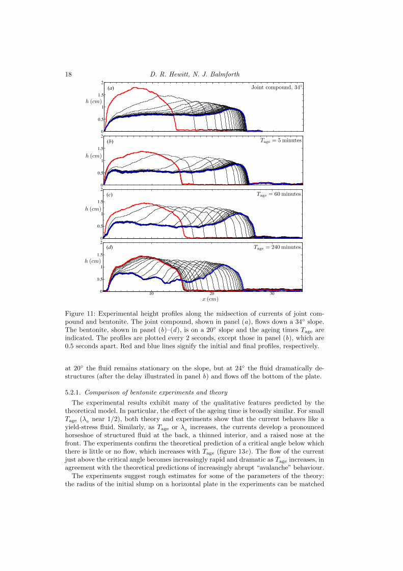
Figure 15: Interfacial instability of a uniform sheet for Γ = 40, λ0

= 0.9, h0 = 1 andY0 = 0.5. Panel (a) shows the unstable (solid) and stable (dashed) roots of the dispersionrelationship (A 5). Panels (b-c) show numerical solutions for h and Y , respectively, froman initial-value problem beginning with the uniform flow plus a small perturbation withwavenumber 8π and the spatial form of the unstable normal mode. The solutions areplotted at each time unit and vertically offset, in a frame moving at a speed V close tothe modal phase speed. Note the different vertical scales in panels (b) and (c). The insetof (a) shows the root-mean-squared values of h−h0 and Y −Y0 against time, along withthe trend of the unstable mode.

are then

∂h

∂t+

∂

∂xF (h, hx, Y ) = 0,

∂Y

∂t+

∂

∂xG(h, hx, Y ) = 0, (A 1a, b)

where

F (h, hx, Y ) =

∫ h

0

u dz = (S − hx)

∫ Y

0

(h− z)2 (1− λ) (1− λ/λ0) dz, (A 2)

G(h, hx, Y ) =

∫ Y

0

u dz = (S − hx)

∫ Y

0

(h− z) (Y − z) (1− λ) (1− λ/λ0) dz, (A 3)

and the subscript on hx refers to a partial derivative. The fluxes F and G can be evaluatedanalytically using

λ = λ− =1

2

[1−

(1− 4

Γ (h− z) (S − hx)

)1/2], (A 4)

which comes from (2.5b).Equations (A 1) have the uniform equilibrium solution h = h0 and Y = Y0. Normal-

mode perturbations to this base state of the form eσt+ikx, with wavenumber k and growthrate σ, satisfy a dispersion relationship

σ2 + σ(Ak2 + iBk

)+ iCk3 +Dk2 = 0, (A 5)

where

A =∂F

∂hx, B =

∂F

∂h+∂G

∂Y, C = − ∂G

∂hx

∂F

∂Y, D =

∂G

∂h

∂F

∂Y− ∂G

∂Y

∂F

∂h, (A 6a, b, c, d)

all evaluated at h = h0, Y = Y0, and hx = 0. It follows from (A 5) that Re{σ} = 0 onlyif k = 0; that is, the uniform flow is either unstable or stable for all wavenumbers. Fork � 1, we find the two solutions,

Re{σ1} = −Ak2 +O(1), Re{σ2} =C2 −ABC −A2D

A3+O(k−1). (A 7a, b)


On examining the partial derivatives of F and G in more detail, one can establish that thefirst solution is stable (A > 0) whereas the second can be unstable (if C2−ABC−A2D >0). With a little more effort, one can show that the growth rate of the unstable solutionincreases monotonically from zero at k = 0 up to the constant maximum given by (A 7b),and has finite phase speed c = −Im{σ}/k. With parameter settings guided by the fullslump problem considered in the main text, it turns out that the growth rate of instabilityis typically relatively small in magnitude, rather less than the corresponding phase speed.Hence, the perturbations propagate much faster than they grow. Typical solutions of(A 5) are shown in figure 15(a).

The system (A 1) can also be solved numerically with periodic boundary conditionsto explore the nonlinear dynamics of the interfacial instability, starting from a smallperturbation to the uniform base flow. Figures 15(b-c) shows the results of such an initial-value computation, starting with a perturbation with wavenumber k = 8π, correspondingto 4 waves. The instability develops as predicted by linear theory and is more prominenton the yield surface than on the free surface. In the non-linear regime, the instability leadsto the formation of shocks on the material yield surface, with the same wavenumber asthe original perturbation. These shocks generate high wavenumber oscillations on thescale of the grid, which is likely an artefact of the numerical scheme used to solve theequations.

REFERENCES

Alexandrou, A.N., Constantinou, N. & Georgiou, G. 2009 Shear rejuvanation, aging andshear banding in yield stress fluids. J. Non-Newtonian Fluid Mech. 158, 6–17.

Balmforth, N.J. & Craster, R.V. 1999 A consistent thin-layer theory for Bingham plastics.J. Non-Newtonian Fluid Mech. 84, 65–81.

Balmforth, N.J., Craster, R.V., Perona, P., Rust, A.C. & Sassi, R. 2006a Viscoplasticdam breaks and the Bostwick consistometer. J. Non-Newtonian Fluid Mech. 142, 63–78.

Balmforth, N.J., Craster, R.V., Rust, A.C. & Sassi, R. 2006b Viscoplastic flow over aninclined surface. J. Non-Newtonian Fluid Mech. 139, 103–127.

Balmforth, N.J., Craster, R.V. & Sassi, R. 2002 Shallow viscoplastic flow on an inclinedplane. J. Fluid Mech. 470, 1–29.

Balmforth, N.J., Craster, R.V. & Toniolo, C. 2003 Interfacial instability in non-Newtonian fluid layers. Phys. Fluids 15, 3370–3384.

Barnes, H.A. 1997 Thixotropy — a review. J. Non-Newtonian Fluid Mech. 70, 1–33.Bonn, D., Tanaka, H., Coussot, P. & Meunier, J. 2004 Ageing, shear rejuvenation and

avalanches in soft glassy materials. J. Phys. Condens. Matter 16, S4987–S4992.Chen, K.P. 1993 Wave formation in the gravity-driven low Reynolds number flow of two liquid

films down an inclined plane. Phys. Fluids A 5, 3038.Coussot, P., Nguyen, Q.D., Huynh, H.T. & Bonn, D. 2002a Avalanche behaviour in yield

stress fluids. Phys. Rev. Lett. 88, 175501.Coussot, P., Nguyen, Q.D., Huynh, H.T. & Bonn, D. 2002b Viscosity bifurcation in

thixotropic, yielding fluids. J. Rheol. 46, 573–589.Dullaert, K. & Mewis, J. 2006 A structural kinetics model for thixotropy. J. Non-Newtonian

Fluid Mech. 139, 21–30.Henriquez, J. & Simms, P. 2009 Dynamics imaging and modelling of multilayer deposition of

gold paste tailings. Minerals Engineering 22, 128–139.Huppert, H.E. 1982 The propagation of two-dimensional and axisymmetric viscous gravity

currents over a rigid horizontal surface. J. Fluid Mech. 121, 43–58.Huynh, H.T., Roussel, N. & Coussot, P. 2005 Ageing and free surface flow of a thixotropic

fluid. Phys. Fluids 17, 033101.Khaldoun, A., Moller, P., Fall, A., Wegdam, G., De Leeuw, B., Meheust, Y., Fossum,

J.O. & Bonn, D. 2009 Quick clay and landslides of clayey soils. Phys. Rev. Lett. 103,188301.


Lister, J.R. 1992 Viscous flows down an inclined plane from point and line sources. J. FluidMech. 242, 631–653.

Liu, K.F. & Mei, C.C. 1989 Slow spreading of a sheet of Bingham fluid on an inclined plane.J. Fluid Mech. 207, 505–529.

Mewis, J. & Wagner, N.J. 2009 Thixotropy. Adv. Colloid Interface Sci. 147-148, 214–227.Moller, P., Fall, A., Chikkadi, V., Derks, D. & Bonn, D. 2009 An attempt to categorize

yield stress fluid behaviour. Phil. Trans. R. Soc. A 367, 5139–5155.Moller, P., Mewis, J. & Bonn, D. 2006 Yield stress and thixotropy: on the difficulty of

measuring yield stress in practice. Soft Matter 2, 274–283.Putz, A.M.V. & Burghelea, T.I. 2009 The solid-fluid transition in a yield stress shear thin-

ning physical gel. Rheol. Acta 48, 673–689.Simms, P., Williams, M.P.A., Fitton, T.G. & McPhail, G. 2011 Beaching angles and

evolution of stack geometry for thickened tailings - a review. In Paste 2011 Proceedingsof the 14th International Seminar on Paste and Thickened Tailings, Perth, Australia (ed.R.J. Jewell & A.B. Fourie), pp. 323–338.

Documents

Thixotropic gravity currents - University of British …njb/Research/thixo.pdfUnder consideration for publication in J. Fluid Mech. 1 Thixotropic gravity currents DUNCAN R. HEWITT1