Embed Size (px)
Citation preview

Colliding gravity currents
Jonathan Shin
St. John's College
A dissertation submitted for the degree of Doctor of Philosophy
in the University of Cambridge
June 2001

Preface This dissertation is the result of my own work and includes nothing which is the outcome of
work done in collaboration. No part of this thesis has been submitted for a degree or any
similar qualification at this or any other university.
iii

Acknowledgements I would like to give special thanks to my supervisor, Professor Paul Linden, and my acting
supervisor, Dr Stuart Dalziel, for their invaluable suggestions, assistance and
encouragements. They aroused my interest in fluid mechanics as soon as I arrived in
Cambridge, and it was a real pleasure to work with them. I have learnt much from them in
many inspiring conversations.
I would also like to thank all the people from the Fluid Dynamics Laboratory in DAMTP
for their friendly contact. In particular, I would like to thank Dr John Simpson, whose passion
for gravity currents is contagious. His pioneering work has shown me the many applications
of gravity currents. Finally, I would like to thank my family for their support.
This work was funded by the Natural Environment Research Council and by my family. I
am grateful to the Cambridge European Trust for awarding me a scholarship during the thesis,
and to St-John's College for awarding me a grant during my final year.
This thesis is dedicated to my grandfather, Shin Ki-Young, for his noble inspiration and
wisdom, and to my mother, Shin In-Sook, for her love and support.
v

Abstract This work is devoted to collisions of gravity currents. A gravity current is the spreading of one fluid into another caused by the horizontal density difference between the two fluids. The study focuses on relatively small density differences, which drive gravity currents in many of their geophysical and industrial applications. Examples of colliding gravity currents range from the collision of two sea-breezes, to the collision of dense gases released into the atmosphere during an industrial accident. Very few studies have been done on collisions, and the latter are not well understood. The present study aims at understanding and predicting the initial stages of the flow after these collisions. The thesis also aims at improving the understanding of two better-known, but related flows: gravity currents and internal bores. Internal bores are density-driven flows that travel along the interface between two fluids; they have many geophysical and meteorological applications. In this thesis, new laboratory experiments are combined with novel theoretical models to capture the main features of each of the above problems.
The first part of the thesis studies the release of a gravity current from a lock in a rectangular channel. In such a lock release, a disturbance is always created in addition to the current, and travels in the opposite direction. Earlier steady-state theories have ignored this disturbance, and have tried to predict the motion of the current by focusing on the current side only. They predicted that energy is conserved when the current occupies half the channel depth, but that it is otherwise dissipated above the current. Local dissipative theories are found to present some significant discrepancies with experiments for shallower currents. It is thought that interfacial mixing and bottom friction are unlikely to account for these discrepancies. A new analytic theory is therefore presented, which applies the conservation of mass, momentum and energy to the entire lock release, including the backward disturbance. In contrast to local theories, it is found that energy-conserving solutions are possible for all current depths. The global theory is found to agree very well with experiments for all current depths, suggesting that energy is close to being conserved during the initial stages of a Boussinesq lock release.
The second part of the thesis studies the release of an internal bore from a lock in a rectangular channel. Some new lock-release experiments are reported. It is observed that a disturbance is created in addition to the bore in each lock release. Earlier steady-state theories of internal bores are applied to the lock-release problem. These local theories predict that energy must, in general, be dissipated. They are found, however, to present some significant discrepancies with the new experiments for shallower and stronger bores. A new theory of internal bores is presented, which applies mass, momentum and energy conservation globally. In contrast to local theories, energy-conserving solutions are possible for all bore depths. The global theory agrees well with the new experiments across the whole parameter space, suggesting that energy is close to being conserved.
The third and final part of this thesis studies collisions of gravity currents in a rectangular channel. Two problems are considered: the collision of a single gravity current against a high vertical wall, and the collision of two gravity currents of equal density but different sizes. Building on the improved understanding of gravity currents and internal bores, a global theory is derived for the first problem. An energy-conserving solution is found, which agrees well with earlier experiments. Some new experiments are reported for the collision of two gravity currents. A global theory is also derived for the second collision problem, and is found to agree well with the new experiments.
vii

Contents
1 INTRODUCTION ...............................................................................................................1
1.1 MOTIVATION....................................................................................................................1 1.2 FOCUS OF STUDY..............................................................................................................6 1.3 APPROACH .......................................................................................................................9 1.4 OUTLINE OF THESIS........................................................................................................10
2 EXPERIMENTAL TECHNIQUES.................................................................................13
2.1 INTRODUCTION ..................................................................................................................13 2.2 USE OF EXPERIMENTS TO MODEL ENVIRONMENTAL FLOWS................................................14 2.3 APPARATUS AND VISUALISATION TECHNIQUES ..................................................................16 2.4 SALINITY MEASUREMENTS.................................................................................................19 2.5 EXPERIMENTAL SET-UP AND STRATIFICATION TECHNIQUES ...............................................20
2.5.1 Gravity current experiments .............................................................................20 2.5.2 Internal bore experiments .................................................................................23 2.5.3 Collision experiments .......................................................................................27
2.6 SUMMARY......................................................................................................................28
3 GRAVITY CURRENTS IN LOCK RELEASES ...........................................................29
3.1 INTRODUCTION ..............................................................................................................29 3.2 EXPERIMENTS ................................................................................................................30 3.3 THEORY .........................................................................................................................39
3.3.1 Local theory ......................................................................................................39 3.3.2 Shallow-water theory........................................................................................50 3.3.3 Global theory ....................................................................................................56
3.4 FURTHER CONSIDERATIONS ...........................................................................................67 3.4.1 Validity of local theory.....................................................................................67 3.4.2 Validity of global energy-conserving solution .................................................71
3.5 SUMMARY......................................................................................................................72
4 INTERNAL BORES IN LOCK RELEASES .................................................................75
4.1 INTRODUCTION ..............................................................................................................75 4.2 EXPERIMENTS ................................................................................................................76 4.3 THEORY .........................................................................................................................87
4.3.1 Local theory: energy conservation in the upper layer ......................................87 4.3.2 Local theory: energy conservation in the lower layer ......................................96 4.3.3 Shallow-water theory......................................................................................101 4.3.4 Global theory ..................................................................................................106
ix

4.4 FURTHER CONSIDERATIONS......................................................................................... 117 4.4.1 Validity of local theory .................................................................................. 117 4.4.2 Validity of global energy-conserving solution............................................... 121
4.5 SUMMARY ................................................................................................................... 123
5 COLLIDING GRAVITY CURRENTS ........................................................................ 125
5.1 INTRODUCTION............................................................................................................ 125 5.2 EXPERIMENTS.............................................................................................................. 126
5.2.1 Collision of a gravity current against a wall .................................................. 126 5.2.2 Collision of two gravity currents.................................................................... 128
5.3 THEORY....................................................................................................................... 137 5.3.1 Collision of a gravity current against a wall .................................................. 137 5.3.2 Collision of two gravity currents.................................................................... 144
5.4 SUMMARY ................................................................................................................... 156
6 CONCLUSIONS AND FUTURE WORK .................................................................... 157
6.1 CONCLUSIONS ............................................................................................................. 157 6.2 DISCUSSION AND FUTURE WORK.................................................................................. 160
BIBLIOGRAPHY ................................................................................................................ 163
A EQUIVALENCE OF BERNOULLI'S EQUATIONS ................................................ 171
A.1 GRAVITY CURRENT IN A LOCK RELEASE...................................................................... 171 A.2 INTERNAL BORE IN A LOCK RELEASE .......................................................................... 172 A.3 COLLISION OF GRAVITY CURRENT AGAINST A SOLID WALL......................................... 174
x

1.1 Motivation
Chapter 1
Introduction 1.1 Motivation
The subject of this thesis is the collision of gravity currents. A gravity current, sometimes
called a 'density current', is the spreading of one fluid into another fluid caused by the
horizontal density difference between the two fluids. The flow of a gravity current is
predominantly horizontal, and can occur as either a top or bottom boundary current, or as an
intrusion at some intermediate level. It consists of a 'head' region at the front, which is usually
deeper than the following 'tail'. Although some mixing usually occurs at the head, the clear
distinction between the gravity current and the ambient fluid typically remains. Gravity
currents occur in many geophysical and industrial situations. Natural examples include sea
breezes, avalanches, estuaries (where fresh water meets salt water), surges from volcanoes,
and thunderstorm outflows. Man-made examples include the accidental release into the
atmosphere of dense gases, which can be either toxic or poisonous, and the early stages of an
oil spillage. In his book, Simpson (1997) gives a comprehensive description of gravity
currents in the environment.
In a number of interesting circumstances, two gravity currents can occur in the same region
and collide. The resulting flow produces a complex interaction. Very little is known about
these interactions and their study is important for predicting consequences of geophysical
1

Chapter 1: Introduction
flows and of industrial accidents. An important geophysical example is the collision of two
see-breeze fronts (Clarke, 1984). The sea breeze is caused by diurnal temperature differences
between land and sea. When the sun shines, the sea surface temperature changes very little,
but the land becomes hotter. The resulting temperature contrasts at low levels are responsible
for the onset of the sea breeze. During a clear day, sea breeze fronts travel inland many tens of
kilometres from the coastlines. A collision occurs when two sea breezes propagate in from
two coastlines on either side of a cape or peninsula and meet. Such a collision can affect the
local conditions. Sea breezes indeed play an important role in the temperature, pollution level
and fauna of coastal regions. Firstly, they tend to cool down the inland regions. Secondly, sea
breezes affect the distribution of airborne pollution. They concentrate aerosols and make
possible undesirable chemical changes. In the coastal city of Los Angeles, air can flow inland
as a sea breeze front and become heavily contaminated with the ingredients of photochemical
smog (Stephens, 1975). Such smog has an oxidising power that can be five or six times the
US quality standard for clean air. A similar smog front used to be common in the
Middlesborough coastal district in north-east England. Thirdly, sea breezes play an important
role in the fauna of coastal regions. As a sea-breeze front advances inland, swarms of insects
are lifted into the band of rising air ahead of the front, and birds soaring at the front can find a
continuous supply of food (Lack, 1956).
Another important example of collision, this time of industrial nature, occurs when gravity
currents made of heavy gases collide with each other. Such gases are released into the
atmosphere when containers are accidentally ruptured (Simpson 1997, pp 69-76). The leaking
dense gas spreads into the surroundings as a gravity current and can often be toxic or
explosive. The consequences of such a release can be devastating. Perhaps the most dramatic
example of such a release occurred in 1984 at the Union Carbide plant in Bhopal, India. At
least 4000 people lost their lives when 40 tonnes of methyl isocyanate, a poisonous gas,
leaked from a tank and spread across the nearby shanty town. The full extent of the tragedy
may never be known since the long-term effects of exposure to the chemical are hard to
measure. In certain circumstances, more than one gravity current can be released during an
industrial accident. For example, several containers may be ruptured at the same time, or a
single tank may suffer multiple ruptures. In such events, the resulting gravity currents could
collide with each other, as well as with surrounding obstacles. Such collisions are likely to
change the spread of the two escaping currents, and may involve alternative remedial actions.
2
1.1 Motivation
For example, the collision of two currents may result in a deeper flow. The latter could flow
over obstacles that would have otherwise been high enough to stop the individual currents.
A third example of collision, again of industrial nature, occurs when two oil slicks meet
during an accidental release. In the last two decades, the public has become increasingly
familiar with oil spillage. One of the most recent examples occurred in December 1999 when
the oil tanker 'Erika', chartered by Total-Fina, broke in two off the coast of Brittany. It spilled
about 15,000 tonnes of heavy fuel oil, thereby polluting about 400 kilometres of Europe’s
coastline in France. The oil slicks caused severe damage to fauna, flora, fisheries and tourism
- with implications also for public health. As oil has a lower density than water, it spreads
over the surface of the sea. The initial stages of the slick are similar to the early stages of any
gravity current immediately after release (Fay, 1969; Fannelop & Waldman, 1971; Hoult,
1972). Containment of oil slicks is very difficult. Floating booms are generally used, but
currents, winds and waves usually limit their effectiveness (Wilkinson, 1972). Additional
difficulties can arise when a first oil slick is followed by a second one. A second gravity
current then forms, and can eventually collide with the first current. As for dense gas releases,
the collision can alter the flow and further complicate it. These complications can in some
cases slow down the skimming of the initially contained layer (International Environment
Reporter, 1994). In some places, the flow can also become deep enough as a result of the
collision to flow under the booms already present. These secondary oil slicks are common in
the Russian Arctic region, where sea pipelines are often in poor conditions; the rupture of a
sea pipeline is usually accompanied by several other ruptures. In 1994, a first rupture
occurred near the town of Usinsk in Northern Russia (Lee, 1997). Although an artificial dam
successfully stopped the first spill, secondary ruptures occurred a few days later, resulting in
several oil slicks colliding with each other. The collisions, together with bad weather
conditions, led to the dam breaking and releasing over 100,000 tons of oil into the tundra.
Another important example of collision occurs when two avalanches meet each other as
they travel down a slope. An avalanche often depends on the suspension of solid particles that
are raised above the ground as the avalanche travels down. Suspended airborne snow or
debris particles increase the density of the flow, thereby creating a gravity current. Such
suspension currents are common in the ocean, where they arise as so-called 'turbidity currents'
(Simpson 1997, p. 102). Sedimentary deposits provide evidence for the collision of turbidity
gravity currents in the ocean bed (Simpson 1997, p. 197). Suspension currents are frequent in
3

Chapter 1: Introduction
alpine regions, where snow avalanches can present a real danger to local villages during
certain seasons (Salm, 1982; Hopfinger, 1983). Remedial actions against a snow avalanche
include planting coniferous trees to prevent initial slides, and placing solid fences to stop the
avalanche (Hopfinger & Tochon-Danguy, 1977). However, two or more avalanches are
sometimes formed at the same time, and may collide with each other (Salm, 1966). The
resulting flow can take routes that the individual avalanches could not have taken, thereby
avoiding the security fences. The combined flow can also become high enough to flow over
the otherwise safe fences. In that case, a low fence usually has the effect of accelerating the
flow just above it, and damage can be increased.
As explained by Simpson (1997, p. 197), colliding gravity currents are closely associated
to another type of flow: the 'internal bore'. Internal bores are density-driven flows that travel
along the interface between two fluids, one lying on top of another that is perhaps only a few
percent denser. They appear as disturbances whose passage results in a change of depth in
each of the two layers. Like gravity currents, internal bores mark the leading edge of a
continued transfer of mass. They therefore differ from interfacial waves, whose main effect is
the transport of energy. Internal bores differ from disturbances like rarefaction waves in that
they have a well-defined front, and a finite depth, which is higher than the undisturbed depth
ahead of the bore. The shape of an internal bore does not change in time, and internal bores
are in that respect similar to internal solitary waves. During the last two decades, internal
bores have provided an explanation for an increasing number of phenomena in the
environment, both in the ocean and in the atmosphere. They may for example be formed in
the ocean by tidal effects in estuaries (Cairns, 1967; Winant, 1974). In the Mediterranean Sea,
the effect of evaporation exceeds that of river discharge. The water is therefore more saline in
the Atlantic. As the tide rises, a layer of less saline water flows above a sill in the Strait of
Gibraltar and enters the Mediterranean as an internal bore (Farmer & Armi, 1986). In the
atmosphere, they are formed in dense stable layers, such as those associated with nocturnal or
maritime temperature inversions. Perhaps the most striking manifestation of these internal
bores is the so-called 'Morning Glory', which occurs near the southern coast of the Gulf of
Carpentaria in Northern Australia (Clarke et al., 1981; Smith et al., 1982; Clarke, 1972,
1983). It is described as a type of wind squall that is accompanied by a sharp rise in surface
pressure and a change in wind direction. The Morning Glory is marked by a spectacular roll
of cloud. A study by Rottman & Simpson (1989) shows that internal bores are most probably
formed by the interaction between a gravity current and low-level temperature inversions.
4

1.1 Motivation
This gravity current can be a cold thunderstorm outflow or, in the case of the Morning Glory,
it can be a sea breeze front. As we shall see shortly, internal bores can also be formed during
the collision of two gravity currents.
Very few studies of the collision of two gravity currents have been published so far, and
results have been mostly qualitative. In general, these studies have involved two gravity
currents of different densities. Findlater (1964) and Rider & Simpson (1968) described the
collision between two mesoscale frontal flows in the atmosphere. Findlater observed that the
combination of the rising air at the two current fronts produced an especially strong zone of
convection, thereby confirming that colliding gravity currents have important meteorological
applications. Rider & Simpson observed two disturbances that clearly emerged from the
collision and moved at about the same speed and direction as before the meeting. The
formation of an atmospheric bore from a collision has been confirmed by Wakimoto &
Kingsmill (1995), who examined the meeting of a sea-breeze front and a gust front over
central Florida in August 1991. Using remote-sensing devices they established the three-
dimensional structure of an undular bore that resulted from the collision. Kot & Simpson
(1987) performed a number of laboratory experiments where two gravity currents are released
in a rectangular channel and are made to collide. Their experiments focused on the collision
of two gravity currents that, in general, had different densities as well as different sizes. They
showed that the main effect of a collision is the emergence of two undular bores propagating
in opposite directions, thereby confirming atmospheric observations. The few attempts to
model collisions have only involved numerical simulations. Clarke (1984) developed a two-
dimensional numerical study for the collision of two sea breezes. His numerical simulations
focused on the collision that occurs on the Cape York Peninsula, in Australia, where two sea
breezes propagating inland from the east and west coasts are observed to meet. Clarke's
simulations showed that during such a collision, cool sea-breeze air is forced upward to form
a hump of relatively cool air. This process continues until a condition for bore formation is
met. At that stage, two bores are usually formed, moving at approximately the same speeds as
the two respective sea-breeze fronts before collision. Recent numerical simulations by
Pacheco et al. (2000), confirmed the emergence of two bores from the collision of two gravity
currents. Although numerical simulations have shed some light into some of the processes
that occur in atmospheric collisions, they have not provided any quantitative results for the
more general geophysical and industrial problems mentioned earlier.
5
Chapter 1: Introduction
Another problem of particular interest in this thesis is the collision of a single gravity
current against a solid vertical wall that is much higher than the current. Such a collision
occurs in situations that are similar to those described above. For example, dense gas released
into the atmosphere during an accident could collide against a tall vertical wall. The wall
could be that of a neighbouring container or building, or it could be placed on purpose to
prevent the spreading of dense gas during an accident. Other examples would include an oil
slick colliding against a floating boom that is much deeper than the slick, or an avalanche
colliding against a high solid fence or the wall of a tall house down the slope. Rottman et al.
(1985) and, more recently, Lane-Serff et al. (1995) studied the flow of a gravity current over
an obstacle. Rottman et al. found in laboratory experiments that the current does not spill over
the obstacle when the obstacle height is about twice the current height. They observed that the
current is in that case completely reflected by the wall as an internal bore. The internal bore
has about twice the height of the initial current, and travels at about the same speed as the
current, but in the opposite direction. Rottman et al. provided a simple theory for the problem.
However, their theory is mostly qualitative and does not predict the speed and the height of
the reflected bore.
The above examples show the variety of situations associated with colliding gravity
currents, and the importance of studying such events.
1.2 Focus of study
The ambient fluid through which two gravity currents travel before a collision is not always
uniform in density. For example, the lower atmosphere in which sea breezes travel is usually
stratified: the density of the ambient fluid decreases linearly with height. Nevertheless, the
ambient fluid can often be considered uniform when the density difference that drives the
current is much larger than the change in ambient density over the height of the current. In
atmospheric applications, this approximation is valid when the gravity current heights are
lower than about one kilometre, which is the case for most of the geophysical and industrial
examples given in the previous section (cf. Simpson, 1997). As a result, the ambient fluid in
this study is approximated as a fluid of uniform density.
6

1.2 Focus of study
In some of the situations described in §1.1, the two gravity currents involved in the
collision are of nearly equal density. For example, dense gas (or oil) can be released from two
different ruptures in the same container. Two nearby avalanches colliding can also have
nearly equal density. These situations are essentially two-layer problems as they involve two
different densities (that of the currents and that of the ambient fluid). In other situations, the
two gravity currents involved in the collision can have different densities. For example, the
temperatures on either side of a cape may differ, so that the resulting sea breezes have
different densities. These situations are essentially three-layer problems, as they involve three
different densities (those of each current and that of the ambient fluid). They are generally
more complex than the two-layer problem. As a result, the present thesis concentrates on the
collision of two gravity currents of equal density (but in general of different sizes).
In most of the geophysical and industrial applications described in §1.1, the density
difference driving the gravity current is small relative to the density of the ambient fluid. An
exception is the release of dense gases, which can be several times denser than air
(Gröbelbauer et al., 1993; Rottman et al., 1985, 2001). The limit of density excess in saline
flows in the ocean is about three percent. In the atmosphere, this density difference
corresponds to a temperature difference of 10 K, which is not often exceeded. As a result,
density differences can often be neglected, except when they are coupled with gravity. Fluids
for which such an approximation holds are called 'Boussinesq' fluids. Since many of the
situations that motivate this study involve relatively small density differences, the present
thesis focuses mostly on Boussinesq fluids.
Gravity currents in the environment are, in general, approximately inviscid (Simpson 1997,
p. 11). The relatively minor role played by viscosity is shown by considering the Reynolds
number, which is defined as
ν
ULRe = , (2.1)
where U and L are typical velocity and length scales of the flow, and ν is the kinematic
viscosity. The Reynolds number is the ratio of the advective term to the viscous term in the
momentum equation: the higher the Reynolds number, the lower the effect of viscosity.
Simpson & Britter (1979) showed in laboratory experiments that viscous effects were
negligible when Re is greater than about 1000. In the examples described in §1.1, the
Reynolds numbers are all greater than 1000. In a thunderstorm, Re can be as high as 108, so
7

Chapter 1: Introduction
that viscous effects only play a minor role in the behaviour of the flow. In certain
environmental flows, however, Re is of the order of 10 or lower, and viscosity plays a major
role in the propagation of gravity currents. This is the case in the secondary stages of an oil
spillage, where viscous forces slow the spreading of the slick (Hoult, 1972). Another example
is the lava flow that occurs in the vicinity of a volcano (Huppert, 1982; Huppert et al., 1982).
This thesis focuses on inviscid gravity currents, which include most of the applications that
motivate this study.
In the environment, the collision of two gravity currents is complicated by many factors.
Firstly, external conditions can affect the flow. Strong winds can facilitate or counteract the
propagation of sea breeze fronts, depending on the relative directions of the wind and the
gravity currents (Biggs & Graves, 1962; Watts, 1955). Winds can also affect the dispersion of
dense gases, as was shown during field trials performed at Thorney Island in 1985 (McQuaid,
1985). Similarly, coastal and ocean currents, winds, waves, and turbulence can complicate the
spreading of oil slicks. The local topography can also play a role, especially in the case of
avalanches (Salm, 1966). Secondly, collisions can be head-on, or they can occur at different
angles of impact. It is very difficult to include the above effects into a full collision model. As
a result, the present study concentrates on the simplest case of two gravity currents colliding
in a rectangular channel, along a horizontal boundary. The flow is therefore effectively two-
dimensional, and does not involve any topography. Moreover, the collision is isolated from
external disturbances like wind. Despite the above simplifications, the collision problem
studied in this thesis should prove a useful and important step in the understanding of the
many applications that motivate this thesis. The simpler problem should help to predict the
most important features involved in a collision, before more complicated situations involving
three layers, shear flow or topography can be studied.
8

1.3 Approach
1.3 Approach
The flow in a gravity current is often complex. Small-scale mixing processes between the
ambient fluid and the dense fluid, due to the turbulence, mean that a precise knowledge of all
the details of the flow is hard to obtain. Several approaches have been taken to model the flow
of a single gravity current. These have ranged from simple analytic models to more
complicated models and direct numerical simulations (DNS). Experiments have also played a
particularly valuable role.
Simple analytic models can predict the bulk motion of a gravity current, and give some
insight into the physical processes involved in the flow. However, they cannot capture the
exact details of the motion. They can help to clarify the underlying physics of the problem,
and can often give surprisingly good answers, despite their simplicity. More complicated
models can incorporate greater details, but are often restricted to two dimensions and require
numerical simulations. Mixing is generally included through some form of parameterisation.
Such models include those based on the vorticity equation or the Euler equations. In general,
these models capture the small-scale turbulence, but not the large-scale motion of the fluid.
With the ever-increasing power of computers, it is now becoming possible to perform DNS
calculations in certain situations to solve the full Navier-Stokes equations directly. Such DNS
calculations can model all scales of the flow, but are currently limited to moderate Reynolds
numbers by the computational requirements.
Experiments can help to study problems involving gravity currents, and complement
theoretical models and simulations. They can be laboratory experiments, or measurements
from field trials or natural flows. Experiments have the advantage of including all the details
of the flow, and can be used to check that the models give reasonable predictions.
In a collision of two gravity currents, the flow is complicated by the factors described in
§1.2. Nevertheless, the same three approaches as those described above can be used to model
the collision of two gravity currents. In this thesis, it was chosen to study collisions through
laboratory experiments and simple analytic models. Laboratory experiments played a central
role: experimental observations formed the basis of all the models of density-driven flows that
will be presented. The simple analytic models, despite their relative simplicity, will be shown
to agree well with experiments, and to capture the main features of the problems considered.
9

Chapter 1: Introduction
1.4 Outline of thesis
The aim of the present study is to understand and predict the initial stages of the flow after
two types of collision: the collision of two gravity currents of equal density but different
sizes, and the collision of a single gravity current with a solid vertical wall. As described in
§1.1, colliding gravity currents are associated with two other types of density-driven flow:
gravity currents and internal bores. Indeed, gravity currents are present before the collisions,
and internal bores emerge from the collisions. A good understanding of these two types of
flow is therefore necessary before proceeding to the more complicated problem of a collision.
Gravity currents and internal bores are studied in chapter 3 and 4, respectively. Building on
those results, the two collision problems are then studied in chapter 5.
Chapter 2 explains the use and applicability of laboratory experiments to model
environmental flows of a larger scale. Three types of density-driven flows are created in the
laboratory experiments of this thesis: gravity currents, internal bores and collisions of two
gravity currents. The experimental apparatus and the various techniques used in each type of
experiment are described in detail. In all three types of experiments, the flow is created
through so-called 'lock releases'. In a gravity current experiment, a reservoir of dense fluid is
released into a lighter and uniform ambient fluid. This event is representative of the
catastrophic rupture of a large container, leading to the sudden release of a large amount of
dense fluid. In an internal bore experiment, a reservoir of dense fluid is released into a two-
layer stratification. The density of the lower layer is the same as that of the dense fluid in the
reservoir, so that the release is a two-layer problem. After its release, the dense fluid inside
the reservoir forms a disturbance that travels along the interface between the two ambient
fluids. These internal bore experiments differ from those of previous authors, and offer an
alternative way to simulate the creation of an internal bore in the atmosphere. Finally, in a
collision experiment, two gravity currents are released from two separate lock releases and are
made to collide.
Chapter 3 considers the problem of a gravity current released into a uniform ambient fluid
initially at rest. Many models have been published to study this problem. The most notable
models are Benjamin's (1968) steady-state analysis and Rottman & Simpson's (1983) shallow-
10

1.4 Outline of thesis
water analysis. The two models are presented. When applied to lock releases, Benjamin's
steady-state analysis is 'local' in that it attempts to model only a limited part of the flow,
namely the current front, without taking the rest of the flow into account. Rottman &
Simpson's shallow-water model, on the other hand, is 'global' in that it tries to model all parts
of the lock release together. An extra equation is however needed to close the problem.
Rottman & Simpson found that Benjamin's local analysis of gravity currents does not agree in
general with shallow-water theory and lock-release experiments. The discrepancy is
particularly significant for shallower currents. Since a good understanding of gravity currents
is necessary before studying their collisions, a new theory of gravity currents is presented.
The new theory is global in that it applies conservation of mass, momentum and energy to the
entire lock release, rather than only across the current front. It is compared with both
laboratory experiments and shallow-water theory.
Chapter 4 considers the problem of an internal bore released into an ambient fluid initially
at rest. Many models of internal bores have been published. The most notable models for
internal bores are the steady-state analyses of Wood & Simpson's (1984) and Klemp et al.'s
(1997), which are both presented. They have been applied to model internal bores created by
towing a solid object through a two-layer stratification. This problem is however quite
different from the lock release problem considered in this thesis. When applied to the lock
release problem, the above steady-state theories can only model a limited part of the flow,
namely the bore front; they do not take the initial conditions into account. The two models are
compared with some new internal bore lock-release experiments, and with shallow-water
theory. A discrepancy similar to that for gravity currents is found. Since a good understanding
of internal bores is necessary before studying the collision of two gravity currents, a new
global theory of internal bores is presented. Again, the conservation of mass, momentum and
energy is applied to the lock release as a whole. The new theory is compared with the new
lock-release experiments and shallow-water theory.
Chapter 5 looks at collisions of gravity currents, building on the improved understanding
of gravity currents and internal bores developed in chapters 3 and 4. Two types of collisions
are considered. Firstly, the problem of a gravity current colliding against a solid vertical wall
is considered. A new global theory is derived and compared with previous experiments by
Rottman et al.(1985). Secondly, the collision of two gravity currents of equal density but
11

Chapter 1: Introduction
different sizes is considered. A new global theory is derived, and compared with some new
lock-release experiments.
Chapter 6 draws conclusions from the work presented in this thesis. Some ideas for future
extensions are suggested.
12

2.1 Introduction
Chapter 2
Experimental techniques 2.1 Introduction
Laboratory experiments form an essential part of this thesis. All the theoretical models
developed in this study were indeed inspired by experimental observations. The use of
experiments to model environmental flows is first discussed in §2.2. Experiments were
recorded on camera, and images were then digitalised to allow measurements and data
analysis. These visualisation techniques are described in §2.3, together with the apparatus in
which the experiments were performed. Salinity was measured before each experiment, so as
to quantify the density differences that drive the flows. These salinity measurements are
discussed in §2.4. Almost all the experiments performed in this thesis involved a two-layer
stratification. The experimental set-ups and the techniques used to form these stratifications
are described in §2.5. The chapter is briefly summarised in §2.6.
13

Chapter 2: Experimental techniques
2.2 Use of experiments to model environmental flows
Laboratory experiments have long been used to model atmospheric and oceanic flows of a
larger scale, such as those that were described in chapter 1. They are usually preferred to
large-scale field trials for several reasons. First, laboratory experiments are carried out in a
more controlled environment than large-scale field experiments. This means that more data of
a higher quality can be collected. The enhanced control also means that the effect of a
particular aspect of the flow can be separated and carefully studied for a more complete
understanding. Second, laboratory experiments are easily repeatable, either with the same
parameters or for a range of parameters. Finally, field trials are often extremely expensive, or
may even not be possible due to environmental considerations.
Many of the experiments involving buoyancy-driven flows, including those described in
this thesis, are performed using sodium chloride (i.e. common salt) dissolved in water to
generate the buoyancy difference. Experiments using water are much easier to contain and
control than experiments with gas. This makes them safer and easier to conduct. Salt and
water are cheap, readily available and harmless, making them ideal for laboratory use. There
is also a larger range of visualisation and diagnostics techniques available for saline flows
than for gas flows. Some of these will be described in the following sections.
Differences between laboratory and field experiments can arise because of the differing
scales involved. In order to maintain dynamic similarity between laboratory and field
experiments, it is desirable to maintain the relative importance of the terms in the momentum
equation. Possibly the most important dimensionless group of terms to keep constant is the
Reynolds number, which was defined in chapter 1 as
ν
ULRe = , (2.1)
where U and L are typical velocity and length scales of the flow, and ν is the kinematic
viscosity. In the laboratory, the length scale tends to be smaller than in the environment,
thereby reducing the Reynolds number. This problem is eased to some extent by the use of
water, rather than gas, in laboratory experiments. The kinematic viscosity of pure water is
0.01 cm2 s-1 at 20o C, compared to 0.15 cm2 s-1 for air. Simpson (1997, pp. 11 and 213)
showed that the flow is only weakly dependent on the Reynolds number when the latter is
14

2.2 Use of experiments to model environmental flows
greater than about 1000. Viscous effects are in that case negligible. All experiments reported
in this thesis had a Reynolds number larger than 1000, so that flow variables depended only
weakly on the Reynolds number.
Another dimensionless group of terms to consider in the momentum equation is the Peclet
number, defined as
,κ
ULPe = (2.2)
where κ is the diffusivity of the fluid. In the environment, the diffusivity could be the mass
diffusivity of salt in water, for example, or the heat diffusivity. The Peclet number is the ratio
of the advective term to the diffusive term in the momentum equation. Note that the Peclet
number and the Reynolds number only differ by a constant in the denominator. This
difference means that the experimental values of Re and Pe cannot both be the same as in the
modelled atmospheric or oceanic flow. This is because the product UL is already determined
when Re is fixed. However, in most of the applications mentioned in chapter 1, Peclet
numbers are very large (of the order of a few millions), so that diffusion effects are negligible.
In the laboratory experiments performed, Peclet numbers were also very large. The diffusivity
of salt in pure water is 1.1 × 10⁻⁵ cm2 s-1, so that the Peclet number was typically over a
million. The diffusion of salt in water was therefore negligible during the experiments. As
explained in the next section, fresh water and salt solutions were allowed to adjust to room
temperature before running the experiments. Temperature differences were therefore small, so
that heat diffusion could also be neglected.
As explained in chapter 1, many problems in the environment involve Boussinesq fluids,
where the difference in density between the heavier and lighter fluids is small. Saline
solutions are ideal to model those flows. It should be noted, however, that sodium chlorine
cannot be used to create large density differences. The saturation concentration at 20o C is
indeed 312 g per kilogram of water, giving a solution density larger of 1.2 g cm-3. As a result,
density differences larger than twenty percent of the water density cannot be obtained using
NaCl. This thesis focuses on Boussinesq fluids, so the limitation due to saturation does not
cause a problem.
One further difference between water and air is that water is incompressible, whereas air is
not. However, provided the Mach number (the speed of the air flow divided by the speed of
sound) is much lower than one, the compressibility of the air can be neglected (cf. Lamb,
15

Chapter 2: Experimental techniques
1932). This is the case for all the applications considered in this thesis, which were described
in chapter 1.
2.3 Apparatus and visualisation techniques
The experimental work in this thesis is concerned with the release of dense fluid in a
horizontal, rectangular channel. Experiments were carried out in a Perspex tank with
transparent sides. The tank is 200 cm long, 20 cm wide and 25 cm high. The tank was placed
on a large wooden table, and was levelled to within one degree of angle using a spirit level.
Figure 2.1 illustrates the experimental set-up. The initial set-up of the apparatus before each
type of release is described further in §2.5.
500 cm
200 cm
20 cm 25 cm
lampsemi-opaquesheet
camera
table
Perspextank
Figure 2.1. Experimental set-up and apparatus.
Visualisation techniques provide the primary source of information about the flow. The
techniques are all based on the use of video equipment to record the experiment. A colour
CCD camera (Panasonic F10) was used to capture the experiments. It was mounted on a
tripod and placed at a distance of about five metres in front of the tank, so that parallax effects
16

2.3 Apparatus and visualisation techniques
could be neglected (cf. figure 2.1). The camera zoom was arranged so as to view the entire
tank at once. This zoom was appropriate for the present study, which focused on the large-
scale structure of the fluid rather than its details. Moreover, in collision experiments, which
will be described in §2.5, it was necessary to follow the flow near the sidewalls as well as in
the middle of the tank.
Coloured dye is often used to visualise experiments. As light passes through the dye,
wavelengths of the complementary colours are absorbed preferentially. The change in colour
and net attenuation can be used to make qualitative, as well as quantitative measurements. In
this thesis, blue or red food colouring was added to dense solutions so as to distinguish them
from the ambient stratification. In experiments where two gravity currents were released, each
current was dyed with a different colour, so as to also distinguish them from one another. A
long, white lamp was placed behind the tank to provide stronger contrasts between the layers.
A diffuse plastic sheet was placed at the back of the tank, so as to render the illumination
behind the tank uniform.
The output of the colour camera was connected by composite video to a Panasonic AG-
7350 video recorder. The majority of the experiments were recorded onto SVHS videotape to
allow later replay and analysis. The luminescence component of the SVHS video signal was
connected to a PC fitted with a frame grabber card (Data Translation DT2862) and the
DigImage image processing software (Dalziel, 1992). This allowed video images to be
captured directly from the camera during an experiment, or afterwards from the videotape.
The DigImage software allows a 'world' co-ordinate system to be set up to relate the pixel
co-ordinates of the image to the actual physical co-ordinates in the tank. A vertical grid of
known size was placed along the side the tank and used to define the world co-ordinates. A
linear mapping was used to convert between images and co-ordinates. The coefficients in the
mapping were determined by fitting the mapping to a series of known reference points using
the method of least squares. For each image subsequently analysed, the position of any
particular feature or edge of the flow could be measured in the world co-ordinates. In
particular, the height of the interface between two layers could be measured. The spatial
accuracy of the digitised images was limited mostly by the camera to ± 0.5 cm. Some
additional uncertainty in height measurements resulted however from the fact that interfaces
are never completely sharp. This is because some mixing occurs during experiments near the
17

Chapter 2: Experimental techniques
interfaces during the set-up, resulting in an interface thickness of less than about 0.5 cm (see
§2.5).
When studying a fluid flow, one of the most important variables to be measured is the
interface velocity. Methods for measuring the velocity are often based on the inclusion of a
passive marker in the flow that can be followed visually. As mentioned earlier, the method
that was used in this thesis involved the use of a food dye as a tracer. A small amount of dye
was inserted, then mixed into the dense solutions before the latter were added into the tank.
As the dense fluid moved, fronts of dense regions could be followed. To improve the
accuracy of the results and reduce the problems caused by imperfect interfaces due to mixing,
the process of measuring a front velocity was automated using a DigImage command file.
Each image was corrected for the background intensity to ensure that changes in intensity
were due to changes in the dye concentration, and not to spatial changes in the illumination. A
given intensity contour, chosen as the threshold for the dyed region, was traced on each
image. The level of the intensity was chosen so that it was near the background zero intensity,
but above the level of the noise in the background level. The threshold intensity was about
1/20th of the peak intensity in the dyed region, and provided a good indication of the edge of
the dyed region. A minimum contour length was set for the contours to filter out small
patches of high intensity caused by reflections, waves or noise. The maximum upslope
position of the contour was then taken as the position of the front. The DigImage software
provided a much simpler, more efficient and more objective method of creating a distance-
time graph than performing measurements by hand. Front speeds were calculated by fitting a
power law curve to the front position data and differentiating the resulting expression to
obtain the speed. This helped to smooth out any errors in the measurement of the front
position. The deviation from the fitted curve gives an estimate of the error associated with the
calculated speed.
The speeds measured using the above technique were in the range of 4 cm s-1 to 15 cm s-1,
over which the video equipment was adequate for the zoom chosen. For speeds much larger
than those encountered in the present study, a small time interval would be needed to ensure
accurate spatial resolutions. The use of high-speed video equipment would be in that case
necessary. For speeds much lower than those encountered in this thesis, the rate at which the
dye diffuses can become significant, leading to inaccurate measurements of the fluid speed.
This is a fundamental problem with the use of a diffusive marker to measure fluid velocity.
18

2.4 Salinity measurements
As explained in the previous section, the speeds in the experiments performed were
sufficiently high that diffusion was not a significant problem.
The internal structure of the velocity field of a gravity current was recently investigated by
Thomas & Dalziel (2000). They placed neutrally buoyant particles in the flow, and followed
their progress using a variety of particle tracking and particle image velocimetry (PIV)
techniques. The internal structure of the velocity field are beyond the scope of this thesis, and
particle tracking was therefore not used in the present study.
2.4 Salinity measurements
Buoyancy is the primary force driving the flows in the experiments performed in this thesis.
As explained in §2.2, density differences are created by dissolving sodium chlorine in fresh
water. To control such experiments and interpret the data, it is essential to know the density of
the fluids being used. The weight of salt needed to prepare saline solutions of a given density
can be looked up in standard reference tables. Solutions can be made to the required density
by carefully measuring the weight of salt needed, and adding it to a known volume of water.
It is, however, difficult to obtain the right density using this method for two reasons. First, the
volume of water in which salt is dissolved is known only to a few percent. Second, the salt
used during experiments is never pure, and is likely to contain a certain amount of water. As a
result, it is desirable to be able to measure the density of a solution.
A variety of techniques can be used to measure the density of a solution. One of the
simplest techniques is to measure the refractive index of the solution, as the index depends on
the concentration of salt. Tables of density against refractive index for saline solutions are
commonly available. The refractive index can be measured using a refractometer, and can be
calculated by measuring the angle of total internal reflection between the fluid and a solid
prism. Refractometers come in both optical and electronic forms. In optical refractometers,
the refractive index is read from a scale. Electronic refractometers, on the other hand, give a
reading in Brix, which is related to the percentage of sugar in the solution, but is again a
measure of the refractive index. Standard tables can be used to deduce the density of a
solution from the value in Brix. Electronic refractometers are usually designed for medical
use. In the experiments carried out in this thesis, an electronic refractometer was used to
19

Chapter 2: Experimental techniques
measure the density of the salt solutions before each experiment. The error associated with the
refractometer was 0.1 Brix, which is equivalent to about 5 × 10 -4 g cm -3. A low value for the
density difference between the denser fluid and the ambient density in the experiments would
be 10 -2 g cm -3. The error in measuring density differences was therefore always smaller than
about five percent.
Note that the refractive index depends in general on the temperature of the solution. The
electronic refractometer used in the measurements was temperature-compensated, so that
first-order density changes due to temperature could be neglected. In addition, both the fresh
water and any saline solutions used were allowed to adjust to room temperature before
running any experiment. As a result, second-order changes in density due to temperature
differences were also negligible.
2.5 Experimental set-ups and stratification techniques
Three types of experiments were performed in this thesis: the release of a uniform gravity
current, the release of an internal bore, and the release of two uniform gravity currents that are
made to collide. All experiments involved fluids stratified in two layers. When setting up the
experiments, various stratification techniques were used to achieve the initial conditions.
These methods varied with the type of experiment, and are outlined in the following sections,
together with the experimental set-ups.
2.5.1 Gravity current experiments
Figure 2.2 depicts the initial set-up of a gravity current experiment. Dense fluid of height h1
and density ρ1 lies behind a watertight gate. Fresh water of density ρ2 lies on top of the dense
fluid, as well as in front of the gate, so that the total height of fluid is everywhere equal to H.
In order to achieve this set-up, the tank was initially filled with tap water. The watertight gate
was inserted at a certain distance from one of the endwalls. To prevent the gate from slipping,
clamps were fixed on both sides of the gate. Two different methods could then be used to
achieve the stratification.
20

2.5 Experimental set-ups and stratification techniques
Perspex tank watertight gate
h1
Hρ1
ρ2ρ2
Figure 2.2. Initial set-up for gravity current experiments.
In the first method, salt was added behind the gate, so as to obtain a dense solution of
density ρ1 (figure 2.3a). A sheet of foam suspended in a polystyrene float was placed on top
of the dense solution, and fresh water was then poured onto it (figure 2.3b). This technique
has been widely used by previous authors (e.g. Simpson & Britter, 1979; Rottman &
Simpson, 1983). It allows forming a layer of fresh water on top of a layer of denser fluid.
float
h1
Hρ1
ρ2 ρ2
h1ρ1 ρ2 h1
(a)
(b)
Figure 2.3. Experimental steps to achieve the initial set-up shown in fig. 2.2 when α1 ≤ 0.5 : float
technique.
21

Chapter 2: Experimental techniques
In the second method, a vertical rubber hose with a small piece of foam at its end was
attached along the endwall behind the gate (see figure 2.4a). Salt solution of density ρ1,
initially contained in a bucket, was then slowly siphoned into the bottom of the tank via the
hose (figure 2.4b). This second (and new) method allows a layer of dense fluid to form under
a layer of fresh water.
h1
Hρ1
ρ2 ρ2
ρ2 ρ2
foam
rubber hose
bucket
table
(a)
(b)
Figure 2.4. Experimental steps to follow in order to achieve the initial set-up shown in fig. 2.2 when
α1 > 0.5 : hose technique.
In both the first and the second method, light or dense fluid was progressively added
behind the gate until the total height of fluid was equal to H. At the same time, fresh water
was progressively poured in front of the gate, so that the final height of fresh water in front of
the gate was also equal to H. The total heights of fluid on both sides of the gate had to be
close to each other at all times. When they differed by more than about two centimetres, the
difference in pressure between both sides of the gate was large enough to create some leaks
during the set-up.
The method used in a given experiment was selected on the basis of minimising the set-up
time of the experiment, so that diffusion between the two layers behind the gate could be
neglected. At the same time, care had to be taken not to disrupt the interface significantly.
22

2.5 Experimental set-ups and stratification techniques
Interfaces less than 5 mm thick were typically produced this way. The speed at which a layer
of light or dense fluid of given thickness could be formed without significantly disrupting the
interface was roughly the same in both methods. As a result, the method used in a given
experiment depended mostly on the thickness of the layer to form. The float method was used
when the initial height h1 of dense fluid behind the gate was greater than half the total height
H of fluid. In this case, adding a layer of fresh water took less time than adding a layer of
dense fluid. The hose method was used when h1 was lower than . In this case, adding a
layer of dense fluid took less time than adding a layer of light fluid.
2/H
2.5.2 Internal bore experiments
Figure 2.5 depicts the initial set-up of an internal bore experiment. Dense fluid of height h1
and density ρ1 lies behind a watertight gate. A shallower layer of the same dense fluid lies in
front of the gate and has depth h2. Fresh water of density ρ2 lies on top of the dense fluid, so
that the total height of fluid on both sides of the gate is H. In order to achieve this set-up, the
tank was initially filled with fresh water. The watertight gate was inserted at a certain distance
from one of the endwalls. Clamps were once more added to prevent the gate from slipping.
Different methods could then be used to achieve the stratifications. As for gravity current
experiments, the method used in a given experiment was selected so as to minimise the set-up
time of the experiment, hence the effect of diffusion on the interface, without significantly
disrupting the interface. Interfaces less than 5 mm thick were typically produced this way.
Perspex tank watertight gate
h1
Hρ1
ρ2ρ2
h2 ρ1
Figure 2.5. Initial set-up for internal bore experiments.
23

Chapter 2: Experimental techniques
When h1 and h2 were both greater than , salt was first added in front of the gate to
obtain a dense solution of height h2 and density ρ1 (see figure 2.6a). Fresh water was then
added on top of the dense solution using the float technique described in §2.5.1 (figure 2.6b).
At the same time, some fresh water was poured behind the gate, so as to keep the total heights
of fluid on either side equal. This was to avoid leaks, as explained in §2.5.1. When the total
height of fluid on either side reached h1, salt was added behind the gate to obtain a dense
solution of density ρ1 (figure 2.6c). Finally, some more fresh water was added on both sides
of the gate using floats, until the total height of fluid on either side was equal to H (figure
2.6d).
2/H
ρ2 ρ1h2
ρ2ρ2 ρ1h2h1
(a)
(b)
ρ2
ρ2 ρ1h2
H
ρ2
ρ2 ρ1h2
h1
h1
(c)
(d)
Figure 2.6. Experimental steps to follow in order to achieve the initial set-up shown in fig. 2.5 when α1 > 0.5 and α2 > 0.5.
24

2.5 Experimental set-ups and stratification techniques
When h1 and h2 were both smaller than , a layer of dense fluid of height h2 and
density ρ1 was introduced on both sides of the gate using the hose technique described in
§2.5.1. After the layers were formed, the total height of fluid on both sides of the tank was
equal to H (see figure 2.7a). Then, some more dense fluid was introduced behind the gate,
until the dense layer reached a height h1 (see figure 2.7b). At the same time, fresh water was
slowly siphoned out of the top layer behind the gate, so as to keep the total height of fluid
equal to H on both sides of the gate. The siphoning was performed carefully, so as to produce
negligible disruption to the interface.
2/H
h1
Hρ2 ρ2
ρ2 ρ2
ρ2 ρ2
ρ1
h2h2
H
ρ1
(a)
(b)
(c)
Figure 2.7. Experimental steps to follow in order to achieve the initial set-up shown in fig. 2.5 when α1 ≤ 0.5 and α2 ≤ 0.5.
25

Chapter 2: Experimental techniques
When h1 was greater than , but h2 was smaller than , salt was first added behind
the gate to obtain a dense solution of depth h1 and density ρ1 (see figure 2.8a). Then, a layer of
dense fluid of depth h2 and density ρ1 was added in front of the gate into the bottom of the
tank, using the hose technique described in §2.5.1. At the same time, some more fresh water
was added behind the gate using a float, so as to keep the total height of fluid on both sides of
the gate equal (figure 2.8b).
2/H 2/H
h1
ρ1
h1 ρ1ρ2
h2
ρ2
ρ2ρ1
h1
ρ1
h2
ρ2
ρ2ρ1
h1
ρ1
h2
ρ2
ρ2
ρ1
(a)
(b)
(d)
(c)
Figure 2.8. Experimental steps to follow in order to achieve the initial set-up shown in fig. 2.5 when α1 > 0.5 and α2 ≤ 0.5. If (1-α1) > α2 , the steps to follow are (a), (b) and (c). If, on the other hand, (1-α1) ≤ α2, the steps to follow are (a), (b) and (d).
26
2.5 Experimental set-ups and stratification techniques
The final part of the set-up was performed in two different ways. In some experiments, the
depth of the layer of fresh water behind the gate needed to be greater than h2. Fresh
water was in this case added on both sides, using the float technique (figure 2.8c). In other
experiments, the depth of the layer of fresh water behind the gate needed to be lower
than h2 . Fresh water was in that case siphoned out of the top layers on both sides of the gate
(see figure 2.8d). The siphoning was performed carefully, so as to produce negligible
disruption to the interface and avoid the problems of selective withdrawal.
)( 1hH −
)( 1hH −
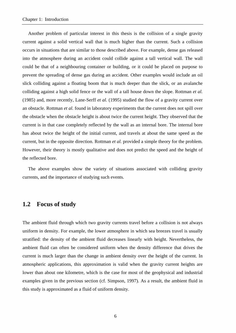
2.5.3 Collision experiments
Figure 2.9 depicts the initial set-up of a collision experiment. Dense fluid of height h1 and
density ρ1 lies behind a first gate (on the left of figure 2.9). A shallower layer of the same
dense fluid lies behind a second gate (on the right of figure 2.9) and has depth h2. Fresh water
of density ρ2 lies on top of the dense fluid and in the middle section between the two gates, so
that the total height of fluid is everywhere equal to H. In order to achieve this set-up, the tank
was initially filled with fresh water. Two watertight gates were inserted at certain distances
from each endwall. Clamps were added to prevent the gates from slipping. The methods used
to set up collision experiments were very similar to those used for internal bore experiments
(cf. §2.5.2). The depths of fluid behind each gate and in the middle section between the two
gates were kept close to each other, so as to prevent the gates from slipping. Fresh water was
therefore regularly added in the middle section.
Perspex tankwatertight gates
h1
Hρ1
ρ2 ρ2
h2 ρ1
ρ2
Figure 2.9. Initial set-up for collision experiments.
27
Chapter 2: Experimental techniques
2.7 Summary
This chapter begins with a brief discussion of the use of laboratory experiments in modelling
environmental flows, focusing on the use of salt water to create density differences. The
various advantages of laboratory experiments over large-scale field trials are outlined.
The apparatus used for the experiments of this thesis is described. Some of the
experimental techniques used are discussed, in particular the visualisation techniques. The
latter provide a large amount of information, enabling heights and velocities of a dense flow,
such as those studied in this thesis, to be measured. The experimental set-up was described for
each type of experiment, together with the stratification techniques. Further details of
individual experiments are given in the following chapters, along with quantitative results.
28

3.1 Introduction
Chapter 3
Gravity currents in lock releases 3.1 Introduction
A 'uniform gravity current' is perhaps the simplest form of gravity current. It travels through
an ambient fluid of uniform density and involves only two layers. Many previous authors
have therefore focused on the uniform case, which is reviewed extensively by Simpson
(1997). This chapter is concerned with uniform currents created by the release of dense fluid
from a lock. The study concentrates on the initial stages of the flow. Some geophysical and
industrial applications of gravity currents were presented in chapter 1. As explained in chapter
1, we focus on inviscid, Boussinesq flows in a rectangular channel.
Previous authors like Simpson & Britter (1979) have used Benjamin's (1968) analysis to
model gravity currents formed in lock releases. Benjamin's analysis was 'local', in that it
focused only on the current side of the flow. It stands in contrast to the 'global' analysis of
Rottman & Simpson (1983), which considered the entire lock release. In general, Benjamin's
local approach may not be appropriate. Firstly, it assumes that the flow on the current side is
independent from that on the other side of the release, which may not be true. Secondly, as
suggested by Rottman & Simpson's shallow-water theory, the local analysis presents some
large discrepancies with experiments in the case of shallow currents. Finally, the local
analysis does not take the initial fractional depth of the current into account, while
29

Chapter 3: Gravity currents in lock releases
experiments show that it is important during the initial stages of the flow (cf. Huppert &
Simpson, 1980). Despite some recent attempt by Klemp et al. (1994) to reconcile local
analysis with shallow-water theory and experiments, these large discrepancies remain.
In §3.2, a qualitative description of lock-release experiments is given. In §3.3, Benjamin's
local model is briefly reviewed, before presenting a new model of uniform currents in lock
releases. The new model will be shown to agree well with both experiments and shallow-
water theory. Some further considerations of the models are discussed in §3.4, and a brief
summary of the chapter is then presented in §3.5.
3.2 Experiments
This section presents qualitative observations of our experiments. Quantitative results are
presented in §3.3, where theories are compared with experiments.
h1
H
ρ1
ρ2
A C
F D
Hρ2
ρ1
u2
A C
F D
u1
E
h1 y1
u3
(a)
(b)
B
B
E
u1
Figure 3.1. Schematic illustration of a lock release in a rectangular channel (a) before release, (b) after
release.
30

3.2 Experiments
Figure 3.1 illustrates an idealised lock release schematically. Dense fluid of height h1 and
density ρ1 lies initially behind lock position E (figure 3.1a). Light fluid of density ρ2 lies on
top of the dense fluid, as well as in front of the lock, so that the total height of fluid on both
sides of the lock position is H. Fluid is initially at rest everywhere, and lies between two
smooth, rigid boundaries. When the dense fluid is released, it forms a uniform gravity current
that moves away from the lock at a constant speed u1 (from left to right in figures 3.1b and
3.1c). A disturbance is also formed, which travels in the opposite direction at constant speed
u3. This problem is similar to the so-called dam-break problem, where fluid is released into air
from rest. The situations after the release in the current frame, where the current is at rest, and
in the disturbance frame, where the disturbance is at rest, are depicted in figures 3.2a and
3.2b, respectively.
Hρ2
ρ1
(u3 - u2)
A
F
u3
E
h1 y1
u3
B
Hρ2
ρ1
D
u1
E
y1
CB
(a)
(b)
(u1 + u3)
(u1 + u2)
P
O Figure 3.2. Schematic illustration of a lock release (a) in the disturbance frame, (b)
in the gravity current frame.
Some previous authors, most notably Simpson & Britter (1979) and Rottman & Simpson
(1983) and Huppert & Simpson (1980), have performed lock releases in the laboratory. To
supplement their study, some new lock-release experiments are reported in this thesis. Gravity
currents were created either individually in 'gravity current experiments', or in pairs in
31

Chapter 3: Gravity currents in lock releases
'collision experiments'.1 The experimental set-up and the techniques used in both types of
experiments were described in chapter 2. Figure 3.3 shows a gravity current created in a lock-
release experiment. Salt water and fresh water were used as dense fluid and light fluid,
respectively, to achieve the initial situation shown in figure 3.3a, which is similar to that
depicted in figure 3.1a. A large number of gravity currents were created (about 130 in total),
covering the range of initial fractional depth 0.17 ≤ α1 ≤ 1, where α1 is defined as
Hh1
1 =α . (3.1)
Our observations of lock releases are very similar to those of Rottman & Simpson and
Huppert & Simpson. In particular, the initial stages of the flow is observed to depend mostly
on the initial parameter α1. When the gate is suddenly removed, the dense fluid behind the
gate forms a uniform gravity current (figure 3.3b). The current moves away from the endwall
at a constant speed. The acceleration from rest to constant speed happens very rapidly, within
a few tenths of a second. Note that the current does not affect fluid far enough ahead, which
remains at rest. As described by Britter & Simpson (1978), Simpson & Britter (1979) and
Simpson (1997), the current has a head and a tail. Mixing between the two fluids is usually
confined near the head via Kelvin-Helmholtz billows, the mixed fluid being left above the
following current tail (Hallworth et al., 1996).
The depth of dense fluid is observed to vary somewhat from the current head to the lock
position. At the head, the current depth ha is observed to be approximately constant in time,
around half the initial height h1 (figure 3.3c). Immediately behind the current head, the depth
hb of dense fluid is usually lower, between a quarter and a third of the initial height. The
current depth then increases from behind the head to the lock position. The depth hc of the
current at the lock position is observed to be about half the initial height h1 at all times. The
interface near the lock position is observed to become more and more horizontal as the
current and disturbance get further apart.
In every lock release, a disturbance is observed to propagate in the opposite direction to
that of the current, i.e. towards the endwall. The leading edge of the disturbance travels at an
approximately constant speed. Fluid ahead of it is not affected and remains at rest. Rottman &
1 Note that although uniform currents formed in pair eventually collide, they do not affect each other before
collision.
32
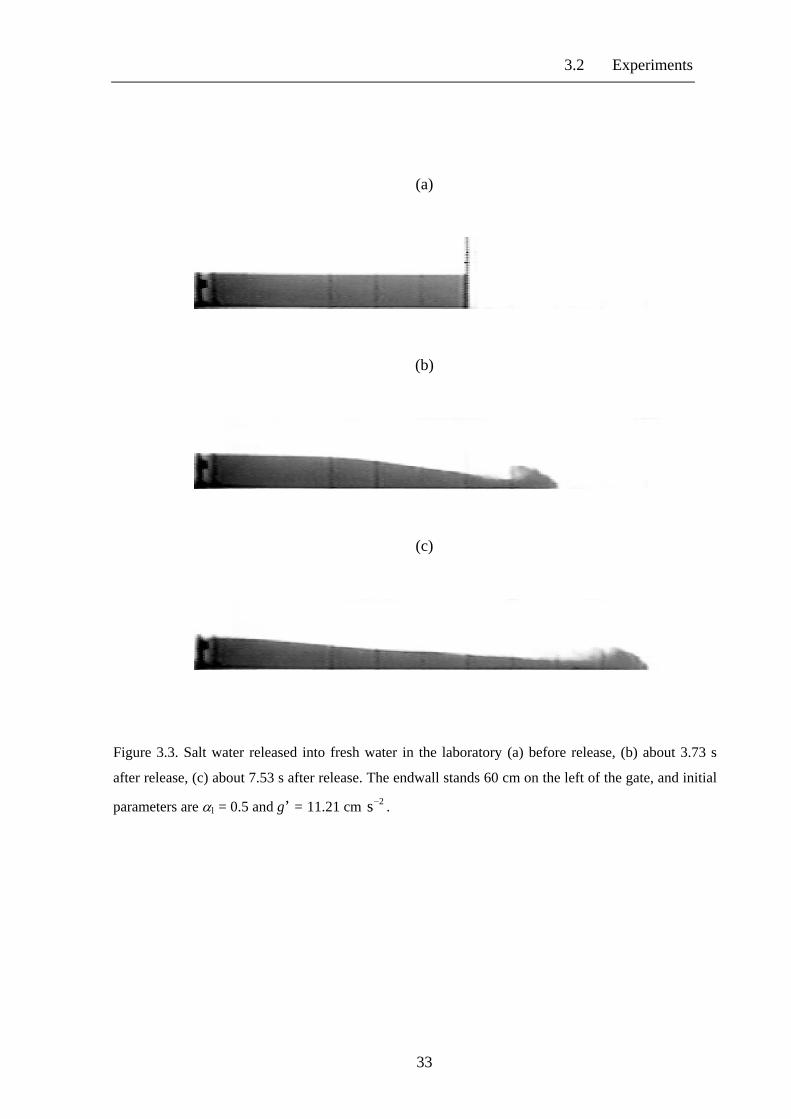
3.2 Experiments
(a)
(b)
(c)
Figure 3.3. Salt water released into fresh water in the laboratory (a) before release, (b) about 3.73 s
after release, (c) about 7.53 s after release. The endwall stands 60 cm on the left of the gate, and initial
parameters are α1 = 0.5 and g’ = 11.21 cm . 2s−
33

Chapter 3: Gravity currents in lock releases
(a)
(b)
(c)
Figure 3.4. Salt water released into fresh water in the laboratory (a) before release, (b) about 2.85 s
after release, (c) about 5.69 s after release. The endwall stands 60 cm on the left of the gate, and initial
parameters are α1 = 0.83 and g’ = 9.75 cm . 2s−
34

3.2 Experiments
(a)
(b)
(c)
Figure 3.5. Salt water released into fresh water in the laboratory (a) before release, (b) about 2.99 s
after release, (c) about 6.15 s after release. The endwall stands about 60 cm on the left of the gate, and
initial parameters are α1 = 1 and g’ = 23.25 cm . 2s−
35

Chapter 3: Gravity currents in lock releases
(a)
(b)
(c)
(d)
Figure 3.6. Salt water released into fresh water in the laboratory (a) before release, (b) about 2.83 s
after release, (c) about 5.47 s after release, (d) about 15.39 s after release. The endwall stands about 20
cm on the left of the gate, and initial parameters are α1 = 0.5 and g’ = 9.81 cm . 2s−
36

3.2 Experiments
Simpson observed that the nature of the backward disturbance depends on the initial
fractional depth α1. For 0 < α1 ≤ 0.7, the backward disturbance is observed to be a rarefaction
wave, while for α1 ≥ 0.8 it forms a type of internal bore, with a rather abrupt change in the
interface level. As described by Baines (1984), a rarefaction wave becomes increasingly
extended in time (cf. left part of figure 3.3), whereas a bore propagates without changing
shape (see left part of figure 3.4). The exact point of transition from rarefaction wave to bore
is difficult to measure. However, as Rottman & Simpson, we observe it to occur somewhere
in the range 8.07.0 1 << α . Mixing is never observed in a rarefaction wave, but it does occur
behind bore fronts when α1 is larger than about 0.8. When the initial fractional depth is equal
to one, the backward disturbance is a uniform gravity current travelling along the surface (see
figure 3.5). This case is called a lock exchange or 'full-depth release' and has been studied
experimentally by Yih (1947, 1965).
The Reynolds number in a lock-release experiment was defined in chapter 1, and is given
here by
ν
11yuRe = , (3.2)
where ν is the kinematic viscosity of the fluid and y1 is the current height. As mentioned by
Klemp et al. (1994), current speeds in Simpson & Britter's experiments are noticeably lower
than those of Rottman & Simpson. Closer inspection of Simpson & Britter's experiments
shows that they have substantially lower Reynolds numbers: all had Re lower than 1000
(detailed data were communicated by John Simpson from DAMTP).2 At those low Reynolds
numbers, bottom friction and viscous forces are not negligible with respect to inertial forces.
As described by Simpson (1967), instabilities form lobes and clefts at the head, reducing the
current speed. As a result, Simpson & Britter measured front speeds in full-depth releases that
were more than fifteen percent lower than the value obtained by Simpson (1997, p. 166) in his
experiments with higher Re. Because of their low Reynolds numbers, Simpson & Britter's
experiments will not be used for comparison in this chapter. In contrast to Simpson & Britter's
experiments, all of Rottman & Simpson's experiments have Re higher than 1000, and all the
2 Simpson & Britter (1979) defined Reynolds number using the height immediately behind the head, which is
about half the depth of the head itself. Following our definition, Simpson & Britter's experiments have Reynolds numbers in the range 600 < Re < 6000. However, only their moving-floor experiments had Re > 1000.
37

Chapter 3: Gravity currents in lock releases
new experiments have Reynolds numbers higher than 2000. Simpson (1997, p. 152) showed
that friction has an effect of less than about five percent on the front speed of gravity currents
for Reynolds numbers larger than 2000.
In practical situations, including laboratory experiments, only a finite volume of fluid is
released. Figure 3.6 shows what happens when the supply of fluid eventually runs out. The
backward disturbance is eventually reflected by the endwall (figure 3.6b). It then propagates
away from the wall with speed slightly greater than that of the current front (figure 3.6c). The
reflection is eventually observed to overtake the front (figure 3.6d). Before the reflected
disturbance overtakes it, the current front moves at a constant speed and with a constant head
height. This initial phase is also called the slumping phase. After the reflection has overtaken
the front, the current falls into a so-called self-similar phase, during which its front speed and
head height decrease with time. As explained by Huppert & Simpson (1980) and Rottman &
Simpson (1983), the front speed during the self-similar phase decreases roughly as 31−t ,
where t is the time after release. After some time, viscous effects dominate inertial effects,
causing the front speed to decrease more rapidly than in the self-similar phase: the current
enters the so-called viscous phase. Fay (1969) and Fannelop & Waldman (1971) used
dimensional analysis to describe the self-similar phase. They assumed that a balance between
inertial and buoyancy forces on the current determines the motion. Hoult (1972) confirmed
their results by deducing the long-time behaviour from a self-similar solution of the shallow-
water equations. He also described the viscous phase in more detail. Huppert & Simpson
presented a model to explain both the self-similar and the viscous phase.
The distance travelled by the current before self-similar phase starts is observed to depend
on the initial fractional depth and on the lock length, i.e. the distance between the lock
position and the endwall. The distance travelled varies from about 3 lock lengths for
17.01 =α to about 9 lock lengths for , in agreement with Rottman & Simpson's (1983)
observations.
)( tu f
This chapter concentrates on the initial phase of lock releases, before reflections on the
endwall overtake the front. Many gravity current experiments were therefore performed with
relatively long lock lengths, from about a quarter to about half the length of the tank. This
allowed us to study the initial phase over a longer distance.
38

3.3 Theory
3.3 Theory
To model lock-release currents, most previous authors have considered the current side as
independent from the disturbance side. Assuming this is true, Benjamin's (1968) local theory,
where the current is considered of infinite horizontal extent, should be applicable. In §3.3.1,
the local theory is reviewed and compared with experiments. In §3.3.2, Rottman & Simpson's
(1983) two-layer shallow-water theory is presented. Benjamin's local theory will be shown to
present, in general, some significant discrepancies with experiments and shallow-water
theory. A new theory is therefore presented in §3.3.3, which considers both the current and
the disturbance side. The global theory will be shown to agree well with both experiments and
shallow-water theory.
3.3.1 Local theory
3.3.1.1 Analysis
As is usually understood, a gravity current consists of dense fluid entering a lighter expanse
of fluid. Benjamin (1968) developed a steady-state theory of uniform gravity currents,
focusing on inviscid, incompressible and immiscible flow. He pointed out that under the latter
conditions the problem is the same as that of an empty cavity advancing along the upper
boundary of a liquid, except for a multiplying factor in front of the gravity constant. Benjamin
chose to consider the cavity problem because of its simplicity. In this section, Benjamin's
theory is applied immediately to the original problem, i.e. that of a dense current entering a
lighter one. Although the analysis presented in this section is slightly less simple than that of a
cavity flow, the chosen presentation will simplify the discussion. Firstly, it avoids some
confusion, as all the experiments presented in this chapter involved gravity currents travelling
along a bottom boundary. Secondly, it introduces some concepts that will be used in the next
section, where a new theory of uniform currents travelling along a bottom boundary will be
presented.
The problem studied in this chapter was presented at the beginning of §3.2. This section
concentrates on the gravity current side of the lock release (cf. the right part of figure 3.1b). In
the gravity current frame, the current front is at rest and the flow is assumed to be steady (cf.
figure 3.2b). Light fluid has uniform speed u1 far upstream (cf. right part of figure 3.2b), and
39
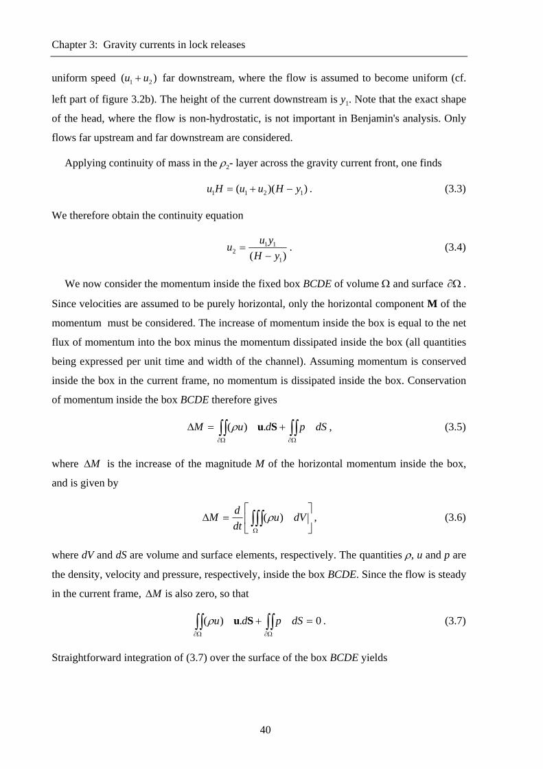
Chapter 3: Gravity currents in lock releases
uniform speed far downstream, where the flow is assumed to become uniform (cf.
left part of figure 3.2b). The height of the current downstream is y1. Note that the exact shape
of the head, where the flow is non-hydrostatic, is not important in Benjamin's analysis. Only
flows far upstream and far downstream are considered.
)( 21 uu +
Applying continuity of mass in the ρ2- layer across the gravity current front, one finds
))(( 1211 yHuuHu −+= . (3.3)
We therefore obtain the continuity equation
)( 1
112 yH
yuu−
= . (3.4)
We now consider the momentum inside the fixed box BCDE of volume Ω and surface Ω∂ .
Since velocities are assumed to be purely horizontal, only the horizontal component M of the
momentum must be considered. The increase of momentum inside the box is equal to the net
flux of momentum into the box minus the momentum dissipated inside the box (all quantities
being expressed per unit time and width of the channel). Assuming momentum is conserved
inside the box in the current frame, no momentum is dissipated inside the box. Conservation
of momentum inside the box BCDE therefore gives
, (3.5) ∫∫∫∫Ω∂Ω∂
+=Δ dSpduM Su.)(ρ
where MΔ is the increase of the magnitude M of the horizontal momentum inside the box,
and is given by
⎥⎦
⎤⎢⎣
⎡=Δ ∫∫∫
Ω
dVudtdM )(ρ , (3.6)
where dV and dS are volume and surface elements, respectively. The quantities ρ, u and p are
the density, velocity and pressure, respectively, inside the box BCDE. Since the flow is steady
in the current frame, MΔ is also zero, so that
0 . (3.7) .)( =+ ∫∫∫∫Ω∂Ω∂
dSpdu Suρ
Straightforward integration of (3.7) over the surface of the box BCDE yields
40

3.3 Theory
,0
2)(
2)(
2)()(
21
1112
21
2
2
212
212212
=⎥⎦
⎤⎢⎣
⎡+−+
−+−
−⎥⎦
⎤⎢⎣
⎡++−+−
ygyyHgyHgp
HgHpyHuuHu
C
B
ρρρ
ρρρ
(3.8)
where pB and pC are the pressures along the top boundary at points B and C, respectively. The
first two terms in (3.8) are the momentum fluxes per unit width of the channel due to fluid
entering the box across CD and leaving the box across BE. The next terms are momentum
fluxes (per unit width) into the box due to pressure forces acting on sides BE and CD. Note
that momentum fluxes across BC and ED are zero. Rearranging equation (3.8), and
substituting for u2 using (3.4) gives
ρρ
ρρ
ρρ
2 12 2
2
212 2
1
2 12
2 1 11 1
2
2 2u H p H
gH u HH y
g H yg H y y
gyBC+ +
⎡
⎣⎢
⎤
⎦⎥ =
−+
−+ − +
⎡
⎣⎢
⎤
⎦⎥Δ
( )( )
( )2
,
(3.9)
where )( BCBC ppp −=Δ . The quantity on the left-hand side of (3.9) is the flow force across
CD, and the quantity on the right-hand side is the flow force across BE. Equation (3.9) shows
that the two flow forces are equal, as explained by Benjamin.
Assuming a hydrostatic variation of pressure with depth, pressure differences along top
boundary and bottom boundary are related by
11 ')( ygppp EDBC ρ+−=Δ , (3.10)
where g' is the reduced gravity, defined as
gg1
21 )('ρ
ρρ −= . (3.11)
Point O in figure 3.2b is a stagnation point. Since there is no dissipation along OD, one can
apply Bernoulli's theorem along OD to give
2
)(21
2upp OD ρ−=− , (3.12)
where pO and pD are the pressures along the bottom boundary at points O and D, respectively.
Furthermore, assuming that the flow inside the current has zero velocity in the current frame,
Bernoulli's theorem can be applied along OE to give
41

Chapter 3: Gravity currents in lock releases
OE pp = , (3.13)
where pE is the pressures along the bottom boundary at point E. Combining (3.10), (3.12) and
(3.13), one obtains
11
21
2 '2
ygupBC ρρ +−=Δ . (3.14)
Using (3.4) and (3.14), u2 and ΔpBC can be eliminated from (3.9) to yield
)1(
)2)(1(' 2
11
βρβββρ
+−−
=Hg
u , (3.15)
where β is the current fractional depth, defined as
Hy1=β . (3.16)
Equation (3.15) is Benjamin's momentum equation and represents momentum balance inside
the box BCDE. The current speed can be determined from (3.15) if the current height is
known.
We now look at the energy balance of the flow. The energy balance can be obtained by
applying Newton's second law to the fixed box BCDE and integrating it over the volume of
the box. The increase ΔE of energy inside the box is equal to the net flux of energy into the
box minus the energy dissipated inside the box (all quantities being expressed per unit time
and width of the channel). In the absence of an external source of energy, the energy flux
comes from energy (kinetic and potential) entering and leaving the box through CD and BE,
and from work being done on the box by pressure forces. The energy equation therefore gives
DdSpudgyuE −++=Δ ∫∫∫∫Ω∂Ω∂
Su.)2
(2
ρρ , (3.17)
where
⎥⎦
⎤⎢⎣
⎡+=Δ ∫∫∫
Ω
dVgyudtdE )
2(
2
ρρ , (3.18)
and where D is the energy dissipated inside the box (per unit time and width of the channel),
defined in this chapter as positive. Since the flow is steady in the current frame, so
that
0=ΔE
42

3.3 Theory
∫∫∫∫Ω∂Ω∂
++= dSpudgyuD Su.)2
(2
ρρ . (3.19)
Note that energy fluxes across BC and ED are zero. Integrating the latter equation over the
volume of the box BCDE, the dissipation inside the box is given by
.)(2
)()(2
)(2
)(2
))((2
)(2
21
21
2211
2
21
21
21
2
21
2
2121
221
21
21
2
⎥⎦
⎤⎢⎣
⎡+
−+−−⎥
⎦
⎤⎢⎣
⎡++
++−
−+−++
−=
uuyHguyHpuHgHup
uuyHguHgyHuuuuHuuD
CB ρρ
ρρρρ (3.20)
Using (3.4) and (3.14) to substitute for u2 and ΔpBC , the last equation reduces to
HuyH
HuHuygD 121
221
2111 )(2'
−−= ρρ . (3.21)
Rearranging the last equation gives the energy equation
⎥⎦
⎤⎢⎣
⎡−
−=Hg
uHg
u
Hg
D')1(2''
21
22
11
25
23 β
ρβρ . (3.22)
Combining the energy equation (3.22) with the momentum equation (3.15), one obtains
)1)(1(2
)21(''
21
25
23
1ββ
ββ
ρ +−−
=Hg
u
Hg
D . (3.23)
Benjamin actually derived the energy balance equation (3.23) using a different, though
equivalent, approach to that described above. Rather than applying Newton's second law to a
fixed box and integrating it over the volume of the box, he applied and introduced a uniform
head loss Δ in the upper layer. Benjamin assumed the head loss to be uniform. The total
energy D dissipated per unit time and width of the channel is therefore equal to the head loss
times the volume flux in the upper layer, so that
Δ= HguD 12ρ . (3.24)
The head loss is found by applying Bernoulli's theorem between O and P, which gives
Δ+++
+= ggyuupp PO 212
221
2 2)( ρρρ , (3.25)
43

Chapter 3: Gravity currents in lock releases
where pP is the pressure at point P along the interface. With energy losses chosen to be
positive, the quantity Δ, as defined in (3.25), represents a loss of energy inside the box. If the
pressure is assumed to have a hydrostatic variation with height, then
11gypp EP ρ−= . (3.26)
Combining (3.4), (3.13), (3.25) and (3.26), one obtains
21
221
2112 )(2'
yHHuygg−
−=Δ ρρρ . (3.27)
Using (3.27), equation (3.24) reduces to (3.22). This result is not surprising, as Bernoulli's
theorem is effectively derived by integrating Newton's second law over a uniform volume.
Although applying Bernoulli's theorem is a simpler method to obtain the dissipation in the
case considered in the present section, the alternative integral method presented in this section
will prove useful in §3.3.3 and in the next chapters. More complicated cases than in this
section will be encountered, which require a non-steady analysis, so that Bernoulli's theorem
will not be applicable in its steady form.
The energy dissipation given in (3.23) is plotted in figure 3.7 as a function of β. As pointed
out by Benjamin, it must be zero in order to have a steady state in the current frame in the
absence of an external source of energy. One notices that D is zero only when β equals 0.5 or
0. Thus, in the only non-trivial case, the current must occupy half the space between the two
boundaries if energy is to be conserved and the flow is to be steady, so that
21
=β . (3.28)
Substituting (3.28) into (3.15), the current speed for this energy-conserving solution is given
by
2
11
21
' ρρ
=Hg
u . (3.29)
In the limit where the ambient stratification density tends to zero, (3.29) shows that the speed
of an energy-conserving current travelling along a bottom boundary tends to infinity. As
Benjamin pointed out, this stands in contrast to the speed of a gravity current running along
the top boundary, for which the speed remains constant in the above limit.
44

3.3 Theory
0.000 0.050 0.100 0.150 0.200 0.250 0.300 0.350 0.400 0.450 0.5000.0000
0.0010
0.0020
0.0030
0.0040
0.0050
0.0060
0.0070
0.0080
0.0090
0.0100
0.0110
β
D /
ρ 1g’ 3
/2H
5/2
Figure 3.7. Non-dimensionalised energy dissipation D in Benjamin’s theory as a function of the
current fractional depth β.
As mentioned earlier we are mainly interested in Boussinesq fluids, for which density
differences are relatively small. Using the Boussinesq approximation, where density
differences are neglected except when coupled with gravity, the depth of the energy-
conserving current given in (3.28) remains unchanged. The current therefore still occupies
half the channel depth. On the other hand, the speed of the energy-conserving current, given
in (3.29), reduces to
21
'1 =Hg
u . (3.30)
This is Benjamin's famous energy-conserving solution for a uniform, Boussinesq gravity
current in a rectangular channel. Note that Benjamin's theory shows that, in the Boussinesq
limit, energy-conserving currents running along a bottom boundary and along a top boundary
travel at the same speed. This result was confirmed in laboratory experiments by Yih (1947).
Equation (3.23) shows that D is always positive for β between 0 and 0.5. In other words, in
Benjamin's analysis energy is in general not conserved, but dissipated inside the box in the
absence of an external source of energy in order to have a steady state. To illustrate this,
Benjamin used the case of a very shallow current travelling in a lighter fluid of infinite extent.
45

Chapter 3: Gravity currents in lock releases
In that case, Benjamin pointed out that a net horizontal motive force acts on the box from
downstream to upstream in the current frame. As he explained, this motive force must be
balanced by another force if the flow is to be steady; otherwise, the current would keep on
accelerating forever. The drag associated with the momentum of the upper fluid, however,
cannot balance the motive force. Indeed, as Benjamin further explained, the drag on a smooth,
horizontal, semi-infinite body inside an infinitely deep fluid is zero. Benjamin therefore
concluded that energy must be dissipated inside the box, at least for very shallow currents
with no bottom friction. He argued that this dissipation, in the absence of bottom friction,
occurs in the ambient fluid in the form of interfacial mixing. Benjamin argued however that
momentum is still conserved, so that the momentum equation (3.15) is still valid. Under the
Boussinesq approximation, (3.15) reduces to
)1(
)2)(1('1
ββββ
+−−
=Hg
u . (3.31)
3.3.1.2 Comparison with experiments
The local theory of Benjamin is now compared with experiments. Benjamin defined a Froude
number G as
1
1
' yguG = . (3.32)
From (3.15), Benjamin's theory predicts that G is given by
)1(
)2)(1(β
ββ+
−−=G . (3.33)
For currents travelling under an infinitely deep surrounding, i.e. when β tends to zero, the
previous equation predicts that G is equal to 2 . Some previous authors have measured G for
shallow currents based on atmospheric observations (cf. Simpson 1969; Charba 1974;
Wakimoto 1982; Carbone 1982; Hobbs & Pearsson 1982; Shapiro et al.1985; Nielsen &
Neilly 1990). Although most atmospheric studies ignored the effect of finite depth, G was
generally measured to be significantly below the value of 2 predicted by Benjamin. As
noted by Klemp (1994) however, measurements in these studies varied widely, ranging from
about 0.7-0.8 (Simpson 1969; Wakimoto 1982) to about 1.4 (Carbone 1982).
46
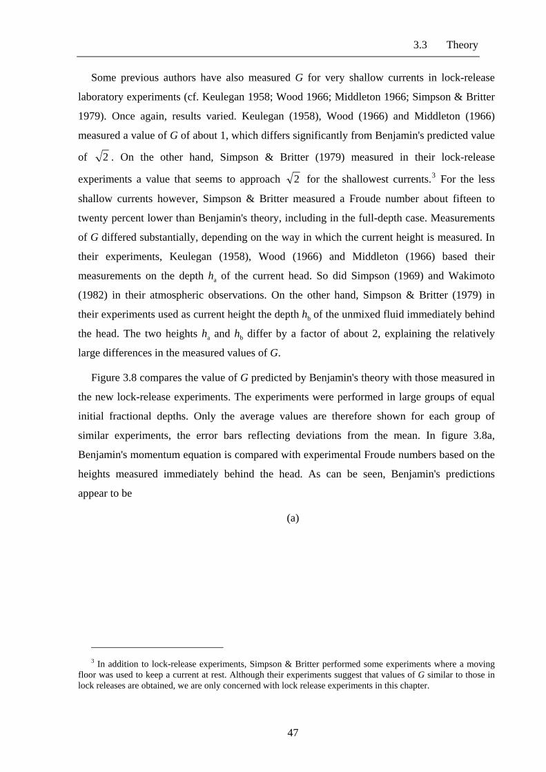
3.3 Theory
Some previous authors have also measured G for very shallow currents in lock-release
laboratory experiments (cf. Keulegan 1958; Wood 1966; Middleton 1966; Simpson & Britter
1979). Once again, results varied. Keulegan (1958), Wood (1966) and Middleton (1966)
measured a value of G of about 1, which differs significantly from Benjamin's predicted value
of 2 . On the other hand, Simpson & Britter (1979) measured in their lock-release
experiments a value that seems to approach 2 for the shallowest currents.3 For the less
shallow currents however, Simpson & Britter measured a Froude number about fifteen to
twenty percent lower than Benjamin's theory, including in the full-depth case. Measurements
of G differed substantially, depending on the way in which the current height is measured. In
their experiments, Keulegan (1958), Wood (1966) and Middleton (1966) based their
measurements on the depth ha of the current head. So did Simpson (1969) and Wakimoto
(1982) in their atmospheric observations. On the other hand, Simpson & Britter (1979) in
their experiments used as current height the depth hb of the unmixed fluid immediately behind
the head. The two heights ha and hb differ by a factor of about 2, explaining the relatively
large differences in the measured values of G.
Figure 3.8 compares the value of G predicted by Benjamin's theory with those measured in
the new lock-release experiments. The experiments were performed in large groups of equal
initial fractional depths. Only the average values are therefore shown for each group of
similar experiments, the error bars reflecting deviations from the mean. In figure 3.8a,
Benjamin's momentum equation is compared with experimental Froude numbers based on the
heights measured immediately behind the head. As can be seen, Benjamin's predictions
appear to be
(a)
3 In addition to lock-release experiments, Simpson & Britter performed some experiments where a moving
floor was used to keep a current at rest. Although their experiments suggest that values of G similar to those in lock releases are obtained, we are only concerned with lock release experiments in this chapter.
47

Chapter 3: Gravity currents in lock releases
0.000 0.050 0.100 0.150 0.200 0.250 0.300 0.350 0.400 0.450 0.5000.00
0.20
0.40
0.60
0.80
1.00
1.20
1.40 experiments, top of head Benjamin’s theory
β
Fa
(b)
0.000 0.050 0.100 0.150 0.200 0.250 0.300 0.350 0.400 0.450 0.5000.00
0.20
0.40
0.60
0.80
1.00
1.20
1.40 experiments, behind head Benjamin’s theory
β
Fb
Figure 3.8. Benjamin's predictions of Froude number compared with experimental Froude numbers based on the current heights measured (a) at the head, (b) immediately behind the head, and (c) at the lock position.
(c)
48

3.3 Theory
0.000 0.050 0.100 0.150 0.200 0.250 0.300 0.350 0.400 0.450 0.5000.00
0.20
0.40
0.60
0.80
1.00
1.20
1.40 experiments, lock position Benjamin’s theory
β
Fc
Figure 3.8. (continued)
in reasonable agreement with experiments. In figure 3.8b, Benjamin's momentum equation is
compared with experimental Froude numbers based on heights measured at the current head.
In this case, Benjamin's theory overestimates Froude numbers measured in experiments. For
the shallower currents predictions differ from experiments by about 50 percent.
The height y1 in (3.15) was defined by Benjamin as the current height far downstream. The
flow downstream was assumed to become uniform so that Bernoulli's theorem could be
applied. Measuring the current height immediately behind the head may therefore not be
appropriate. A better choice of current height may be the depth of dense fluid at the lock
position, which lies further downstream. As described in §3.2, the interface near the lock
position becomes more and more horizontal as the current and disturbance get further apart.
The depth at the lock position may therefore represent Benjamin's downstream current height
more appropriately in a lock release. As seen in figure 3.8c, Benjamin's theory generally
overestimates experimental Froude numbers based on the height at the lock position. For the
shallower currents, Benjamin's predictions differ from experiments by about 40 percent.
49

Chapter 3: Gravity currents in lock releases
Note that Klemp et al. (1994) argued that current fractional depths greater than about 0.35
are not achievable experimentally. Benjamin's half-depth solution was however achieved by
Wilkinson (1982) in his experiments on cavity flows. Current fractional depths around 0.5
were also measured at the front and at the lock position in all full-depth experiments reported
in this chapter. These measurements suggest that Benjamin's half-depth solution can be
achieved in lock-release experiments. The validity of Benjamin’s theory is discussed further
in §3.4.
3.3.2 Two-layer shallow-water theory
3.3.2.1 Analysis
In contrast to Benjamin's steady-state and local analysis, Rottman & Simpson (1983) used
shallow-water theory to study lock releases. They solved the initial-value problem described
in §3.2, which was depicted schematically in figure 3.1. In their analysis, Rottman & Simpson
added a solid vertical wall at a distance L1 behind the lock position. The vertical wall was
introduced to simulate the endwall present in an experiment and allowed them to study the
transition to the self-similar phase. As described in §3.2, the transition is due to the backward
disturbance reflecting on the endwall and catching up with the current front. As mentioned
earlier, the present study is only concerned with the initial phase of a lock release. The
vertical wall is therefore ignored in the following presentation of Rottman & Simpson's
theory, and only the initial phase of the release is considered.
A rectangular co-ordinate system is used with the origin at the lock position and the x-axis
along the bottom horizontal plane. The flow is considered at a time t after the lock is released.
As before, the flow is assumed to be inviscid, incompressible and immiscible. Velocities in
each layer are assumed to be purely horizontal and independent of vertical position. Clearly,
the latter assumption is not valid in the very initial moments of the release, when vertical
accelerations are not negligible. However, as described in §3.2, the flow rapidly accelerates to
a steady speed. The assumption should therefore be valid during most of the initial phase of a
lock release. The shallow-water equations for a two-layer fluid with the above assumptions
are
0)( 111 =
∂∂
+∂∂ yu
xty , (3.34)
50

3.3 Theory
0)( 222 =
∂∂
+∂
∂ yuxt
y , (3.35)
xyg
xp
xuu
tu
∂∂
−∂
∂−=
∂∂
+∂∂ 112
1
11
1 1ρ
, (3.36)
xyg
xp
xuu
tu
∂∂
−∂
∂−=
∂∂
+∂
∂ 112
2
22
2 1ρ
, (3.37)
where p12(x, t) is the pressure at the interface between dense and light fluid, and H is the total
height of the channel, given by
),(),( 21 txytxyH += . (3.38)
Equations (3.34) and (3.35) represent conservation of mass in each layer, and (3.36) and
(3.37) represent conservation of horizontal momentum in a hydrostatic pressure field.
Initial conditions are the same as before. The fluid is initially at rest everywhere. Since
both velocities vanish sufficiently far on the left of the lock position, (3.34), (3.35) and (3.38)
yield
)( 1
112 yH
yuu−
= . (3.39)
Eliminating p12 from (3.36) and (3.37), and substituting for u2 using (3.39), we obtain
( )( ) 0)1('11 1
213
1
211
1
1
1
21
1
2 =∂∂
⎥⎦
⎤⎢⎣
⎡+−+
∂∂
⎥⎦
⎤⎢⎣
⎡−+
−+∂∂
⎟⎟⎠
⎞⎜⎜⎝
⎛+
xy
Huag
xuu
yHyHa
tua
ρρ
ρρ
ρρ , (3.40)
where β=a / ( )β−1 and Hy /1=β . Invoking the Boussinesq approximation, (3.40)
becomes
0')1()21( 111
1 =∂∂
−+∂∂
−+∂∂
xygb
xuua
tu , (3.41)
where
( ) 221 1'
−−+= ββHg
ub . (3.42)
Rottman & Simpson solved the partial differential equations (3.34) and (3.41) for u1 and y1 as
a function of x and t. The system is made of two first-order equations and is therefore of order
two. Two further conditions are required in addition to the known initial state. If the backward
51

Chapter 3: Gravity currents in lock releases
disturbance is a rarefaction wave, the velocity of the dense fluid is zero at the leading edge of
the disturbance, so that
01 =u when 11 hy = . (3.43)
A further condition is required to close the problem. Rottman & Simpson imposed the front
condition
)1(2
)2)(1('
22
βββ
+−−
= cyg
u
f
f , (3.44)
where is the front speed, is the front depth and c is a dimensionless constant. Note
that when , the front condition (3.44) reduces to Benjamin's Froude number equation
(3.15). Note also that a front condition on its own does not give the front speed and height. It
only gives an equation that relates the two variables.
)(tu f )(thf
22 =c
Rottman & Simpson solved the above initial-value problem using the method of
characteristics. This method is described (for example) in Ames (1965, pp. 416-422).
Although this method can be used to give u1 and y1 at any position and time (cf. Ames 1965,
pp. 435-437), we are mainly concerned in this chapter with the current speed and height at the
front. As described by Ames, the solution to (3.34) and (3.41) is equivalent to the solution of
the ordinary differential equations
( ) 021dd
11
11 =±+−− λua
yuy , (3.45)
along characteristic directions specified by
±= λtx
dd , (3.46)
where
[ ]21
)1(')1( 122
11 bygauau −+±−=±λ . (3.47)
Using +λ in (3.46) and (3.47) one can integrate the characteristic equation in the direction of
decreasing y1, subject to the initial condition (3.43), until the front condition (3.44) is
satisfied. This method allows us to determine front speed and height as a function of initial
fractional depth α1.
52

3.3 Theory
3.3.2.2 Comparison with experiments
Figure 3.9a compares the front height hf predicted by shallow-water theory based on
Benjamin's front condition (3.15), which corresponds to in (3.44), with the new
experiments. Heights are measured at the top of the head (ha) and immediately behind the
head (hb). As was seen in the previous section, ha and hb differ by a factor of about two for
shallower currents. A comparison with theory is therefore difficult at lower fractional depths.
Nevertheless, assuming that the front height hf lies between ha and hb, shallow-water theory
based on Benjamin's condition seems consistent with the experiments for all initial fractional
depths.
22 =c
(a)
0.00 0.20 0.40 0.60 0.80 1.000.00
0.10
0.20
0.30
0.40
0.50
0.60
0.70
experimental heights, top of head experimental heights, behind head SWT based on Benjamin’s local theory
α1
h f / h
1
Figure 3.9. Comparison between SWT based on Benjamin’s front condition, and experiments; (a) front heights, (b) front speeds versus initial fractional depth α1.
53

Chapter 3: Gravity currents in lock releases
(b)
0.00 0.20 0.40 0.60 0.80 1.000.00
0.10
0.20
0.30
0.40
0.50
0.60
0.70
0.80
new experiments Rottman Simpson’s experiments SWT based on Benjamin’s local theory
α1
u 1 / (
g’h 1)
1/2
Figure 3.9. (continued)
Figure 3.9b compares the front speed predicted by shallow-water theory based on
Benjamin's dissipative theory, with experiments, including those of Rottman & Simpson's. In
view of the ambiguity associated with measuring the Froude number G defined in (3.32), the
current speed is now non-dimensionalised by the external scale h1
1
1
'hguF = . (3.48)
The Froude number as defined in (3.48) can be measured in lock-release experiments as a
function of the initial fractional depth α1 only. It stands in contrast to the Froude number G,
which depended on the height of the current and was used to compare Benjamin's theory with
experiments. As can be seen from figure 3.9b, front speeds and heights agree with
experiments near the full-depth release. However, Benjamin's theory overestimates the front
speed by about 20 % for shallower currents.
Rottman & Simpson found that, for shallower currents, the front condition (3.44) fitted the
initial phase of their experiments best with . They used the latter condition instead of 12 =c
54

3.3 Theory
Benjamin's condition to describe their experiments for α1 ≤ 0.5. In addition to the initial
phase, Rottman & Simpson also studied the transition to self-similar phase. Although this
thesis is not concerned with the self-similar phase of uniform currents, it is worth mentioning
that Rottman & Simpson found that the transition to self-similar phase was also best described
with , rather than with (Benjamin's condition). 12 =c 22 =c
At initial fractional depths greater than 0.5, Rottman & Simpson (1983) found that their
computed disturbances behaved as internal jumps upon reflection on the endwall. They
therefore suggested that their theory should not be valid for α1 > 0.5. They pointed out
however that no jump was observed in experiments until about α1 ≈ 0.75 (cf. also §3.2). For
this reason, their theory of the initial phase, during which the endwall does not play a role, is
more likely to be valid until about α1 ≈ 0.75. At fractional depth greater than 0.75, the
backward disturbance is a bore rather than a rarefaction wave. The leading edge of the
disturbance is a front, and condition (3.43) does not hold when solving the initial-value
problem.
Shallow-water theory shows that Benjamin's theory overestimates the speed of shallow
currents in lock releases by about 20%. Based on numerical simulations, Klemp et al. (1994)
argued that the large discrepancies can be attributed to both bottom friction and mixing. As
explained in §3.2 however, the new experiments presented in this thesis all have Re > 2000.
The effect of friction on the current speed should be therefore negligible. Moreover, mixing in
stratified fluids has been shown in many theories and experiments to have a limited effect on
the energy balance. This limitation has been shown in contexts as diverse as those of Kelvin-
Helmoltz instabilities (cf. Miles 1961; Thorpe 1973), breaking internal gravity waves (cf.
McEwan 1983) or oscillating grids (cf. Linden 1980; Park et al. 1994). Since mixing in lock-
release experiments can only occur near the interface between dense and lighter fluid, the
effect of mixing on the current speed is expected to be much smaller than in the theories and
experiments above. It is therefore expected in this chapter that the effect of mixing on the
current speed is unlikely to account for the large discrepancies of Benjamin's theory with
experiments. The average front speed (non-dimensionalised with initial height h1) in full-
depth releases was found to be about 0.47, compared to the theoretical value of 0.5 for the
energy-conserving solution. The value in the new experiments agrees with Simpson's (1997,
p. 166) value of 0.465. These values suggest that bottom friction and interfacial mixing
should have a combined effect on the current speed of only six or seven percent. Assuming
55

Chapter 3: Gravity currents in lock releases
that the effects of bottom friction and mixing depend mostly on the Reynolds number, they
should be approximately constant in the new experiments for all values of α1. This is because
all the new experiments are inside the weakly Reynolds-dependent range Re > 2000, as
mentioned earlier. Bottom friction and interfacial mixing should therefore also have a
combined effect on the current speed of only six or seven percent. It is therefore expected that
bottom friction and mixing cannot account for the large discrepancies between Benjamin's
theory and experiments for shallower currents. In light of the discrepancies between the local
theory and experiments, a new theory of lock releases is presented in the next section.
3.3.3 Global theory
In light of the discrepancies that exist between local analysis and experiments, a new theory
of lock releases is presented. Some aspects of the new theory are similar to Benjamin's (1968)
theory, but the new theory applies conservation of mass, momentum and energy globally
rather than locally. To some respect, the new theory is similar to shallow-water theory in that
it considers both sides of the lock release. It nevertheless distinguishes itself from shallow-
water theory by introducing some approximations in order to find analytical rather than
numerical solutions. The analysis of the model is presented in §3.3.3.1. The model is then
compared with lock-release experiments in §3.3.3.2 and with shallow-water theory in
§3.3.3.3.
3.3.3.1 Analysis
The lock release problem was described in §3.2, where densities, velocities and initial heights
were defined (cf. figure 3.1). In the global theory, fluid is assumed to be inviscid, irrotational
and immiscible. Layers are uniform and velocities are purely horizontal. The shape of the
interface is approximated by a horizontal middle section of height y1 and two advancing
fronts. The two fronts are assumed to have a constant shape in time. As in Benjamin's (1968)
analysis, described in chapter 3, the exact shape of the fronts does not matter as long as it
remains steady. The fronts move at speed u1 towards the right and u3 towards the left. A
similar approximation was used in Benjamin's analysis, where the interface was assumed to
become horizontal far downstream of the current. As described in §3.2, the backward
disturbance is in general a rarefaction wave rather than a front of constant shape. The
56

3.3 Theory
interface shape is therefore only an approximation, aimed at simplifying calculations in the
following theory. The validity of the approximation will be examined in more detail in §3.4.
The situations in the current frame and in the disturbance frame after the release were
depicted in figures 3.2a and 3.2b, where current and disturbance fronts, respectively, are at
rest. Applying conservation of mass across the gravity current front and the disturbance front,
one obtains the two independent equations
))(( 1211 yHuuHu −+= , (3.49)
13113 )( yuuhu += . (3.50)
The latter equations give the two continuity equations
)( 1
112 yH
yuu−
= , (3.51)
)( 11
113 yh
yuu−
= . (3.52)
We now consider the momentum balance inside the large fixed box ACDF, which includes
both the current and the disturbance, unlike in §3.3.1. Note that the box is large enough to
include all fluid affected by the lock release at all times. The fluid outside the box is therefore
always at rest. Although velocities and heights are assumed to be constant in this model, the
situation is strictly speaking not steady in the laboratory frame. Unlike in §3.3.1, one cannot
find a frame of reference in which both the current front and the disturbance front are at rest.
Nevertheless, the time-dependent momentum equation (3.5) of §3.3.1 can still be integrated
over the surface of the box. Assuming that momentum is conserved inside the box, no
momentum is dissipated in the absence of external forces. Moreover, since no fluid enters or
leaves the large box in the laboratory frame, the only contribution to momentum flux into the
box comes from pressure forces acting on the sides CD and AF of the box. Momentum
balance (3.5) therefore reduces to
, (3.53) ∫∫Ω∂
=Δ dSpM
where is now the surface of the box ACDF. After integration, the latter equation yields Ω∂
⎥⎦
⎤⎢⎣
⎡+−+
−+−⎥
⎦
⎤⎢⎣
⎡+=Δ 2
11112
21
2
2
2 )(2
)(2
ghhhHghHgHpHgHpM AC ρρρρ (3.54)
57

Chapter 3: Gravity currents in lock releases
where pA and pC are pressures at points A and C, respectively. Using (3.6), the increase of
momentum inside the box ACDF is given by
1131112312 )()()( yuuuyHuuuM +−−+=Δ ρρ , (3.55)
so that (3.54) becomes
,)(
2)(
2
)()()(
211112
21
2
2
2
1131112312
⎥⎦
⎤⎢⎣
⎡+−+
−−⎥
⎦
⎤⎢⎣
⎡+Δ
=+−−+
ghhhHghHgHgHp
yuuuyHuuu
AC ρρρρ
ρρ (3.56)
where . Using (3.51) and (3.52), u2 and u3 can be eliminated from (3.56) to
yield
)( ACAC ppp −=Δ
)(
)(2
'11
112121
21
1 yhhyuhgHpAC −
−−=Δ
ρρρ . (3.57)
Time-dependent Bernoulli's equation can be applied in the top layer to find the pressure
difference between A and C. Assuming that energy is conserved in the top layer, this gives
C
CA
A tp
tp
∂∂
+=∂
∂+ 2
22
2φρφρ , (3.58)
where φ2 is a velocity potential that must be found, such that
topu=∇ 2φ , (3.59)
where u top is the velocity field inside the top layer. The potential function φ2 is required to be
continuous within the whole layer. Since velocities vary only horizontally within each layer,
the last equation reduces to
x
utop ∂∂
= 2φ , (3.60)
where utop is the velocity function in the top layer, given by
utop = 0 for 1xx ≤ (3.61)
u2 for 31 xxx ≤<
58

3.3 Theory
0 for , 3xx >
where x1 and x3 are the positions along the x-axis of the current front and the disturbance
front, respectively. As before, the x-axis is chosen to have its positive direction towards the
left of figure 3.1b. A possible choice of φ2 , which satisfies (3.60) and (3.61) and is continous
for all x, is given by
φ2 = 0 for 1xx ≤ (3.62)
)( 12 xxu − for 31 xxx ≤≤
)( 132 xxu − for . 3xx ≥
Substituing the latter potential function into (3.58), one obtains
)()( 1322 xxuppp ACAC −=−=Δ ρ . (3.63)
Hence, one finds that
)( 3122 uuupAC +=Δ ρ . (3.64)
Note that there is an infinite number of choices for φ2, which all give the same pressure
difference.
Combining (3.51), (3.52), (3.57) and (3.64), one obtains the momentum equation
[ ]βρβρβββααρ
21
11121
)1(2)1)((
' +−−−
=Hg
u , (3.65)
where α1 = h1 / H, α2 = h2 / H and β = y1 / H as before.
We now look at the energy balance of the flow in the laboratory frame. As in §3.3.1 the
balance is obtained by applying Newton's second law, and integrating over the volume of the
box. This time however, the larger fixed box ACDF is used, rather than the fixed box BCDE.
Since no fluid enters or leaves the box through AF, CD, AC or DF, the energy flux into the
box (including contribution from work due to pressure forces) is zero. Equations (3.17) and
(3.18) therefore yield
⎥⎦
⎤⎢⎣
⎡+−= ∫∫∫
Ω
dVgyudtdD )
2(
2
ρρ . (3.66)
59

Chapter 3: Gravity currents in lock releases
The energy D dissipated inside the box ACDF per unit time and width of the channel is
therefore given by
2
)('2
')(2
))((2
21
21
31
21
11311
21
1311
22
2yhugyuguuyuuuyHuD −
+−+−+−−= ρρρρ . (3.67)
Assuming that energy is conserved inside the box ACDF, the energy dissipated per unit time
inside the box is zero. Putting D = 0 in (3.67), one obtains
. (3.68) 0)('')())(( 21
2131
2111311
211311
222 =−+−+−+−− yhugyuguuyuuuyHu ρρρρ
Using continuity equations (3.51) and (3.52) to substitute for u2 and u3 , the energy balance
equation (3.68) reduces to
0)1()(
1)'(' 12
1
21
111 =
⎭⎬⎫
⎩⎨⎧
⎥⎦
⎤⎢⎣
⎡+
−−− ρ
ββρ
βαρβα
Hgu
Hgu . (3.69)
Using the momentum equation (3.65), the energy equation (3.69) reduces to
02
1 111 =⎥
⎦
⎤⎢⎣
⎡−
βαβαu . (3.70)
Thus, in the only non-trivial case, we obtain the energy-conserving solution
2
1αβ = . (3.71)
In other words, when momentum and energy conservation is applied to the box ACDF, the
current height is half the initial height before release. Substituting (3.71) into (3.65), the speed
of the current (non-dimensionalised by the initial height h1) is given by
[ ]1211
11
1
1
)2(2)2(
' αραραρ+−
−=
hgu , (3.72)
and the speed of the backward jump is equal to the current front speed, so that
13 uu = . (3.73)
Using (3.71) and (3.72), the height and speed of the energy-conserving current can be
determined given only the initial fractional depth before release. In contrast to Benjamin's
local theory, applying conservation laws globally does not yield a unique solution regardless
of initial depth. Instead, a whole range of energy-conserving depths 5.00 ≤≤ β is possible,
60

3.3 Theory
depending on the initial fractional depth α1 before release. This means that dissipation need
not be introduced, in contrast to Benjamin's theory. Additional terms on the disturbance side
balance the energy terms on the current side, so that energy can be conserved overall. Energy
conservation is discussed further in §3.4.
The above energy-conserving solution was derived without using the Boussinesq
approximation. It is therefore theoretically valid for any pair of densities ρ1 and ρ2. We expect
however the above model to break down for non-Boussinesq fluids. The model assumes that
the current and disturbance sides can be matched by a flat interface in the middle section,
where velocities are horizontal and conditions are uniform. Although laboratory experiments
show that this assumption should be valid for Boussinesq fluids (cf. §3.2), recent experiments
by Rottman et al. (2001) show that this assumption is wrong for non-Boussinesq gravity
currents. Rottman et al. indeed clearly observe the presence of an internal bore in the middle
section, so that the model assumption of a flat middle section is not valid for non-Boussinesq
fluids. Keller & Chyou (1991) studied the non-Boussinesq lock-exchange problem. Their
theory predicts the presence of such an internal bore in non-Boussinesq lock releases.
Moreover, Keller & Chyou show that the bore should catch up with the current front when the
density ratio ρ1 /ρ2 is larger than about 4, thereby further complicating the problem for highly
non-Boussinesq currents. Laboratory experiments of non-Boussinesq gravity currents have
been performed by Stansby et al. (1998) using water, and by Keller & Chyou and
Gröbelbauer et al. (1993) using gas mixtures. Gröbelbauer et al.’s experiments showed that a
non-Boussinesq gravity current differs significantly in shape from its Boussinesq counterpart.
Stansby et al.’s experiments showed that, in the extreme non-Boussinesq limit of water
released into air, the current head was actually completely suppressed. As explained in
chapter 1, this thesis focuses on situations where density differences are relatively small. For
the latter reason, and in light of the differences between the model and non-Boussinesq
gravity currents, the rest of this chapter will concentrate on Boussinesq currents.
Under the Boussinesq approximation, the momentum equation (3.65) reduces to
β
ββαα2
)1)(('
1121 −−
=Hg
u , (3.74)
and the energy balance equation (3.69) reduces to
61

Chapter 3: Gravity currents in lock releases
0)1)((
1)'(
11
21
11 =⎭⎬⎫
⎩⎨⎧
−−−
ββαβαρ
Hguu , (3.75)
where 21ˆ ρρρ ≈= . For Boussinesq fluids, the gravity current speed given in (3.72) reduces
to
2
)2('
1
1
1 α−=
hgu , (3.76)
and the current height and the disturbance speed are still given by (3.71) and (3.73),
respectively.
As described in §3.2, two gravity currents are formed when 11 =α : one current travels
along the bottom boundary, the other along the top boundary. As one can see, the two currents
in the above Boussinesq solution both tend to Benjamin's energy-conserving solution when
11 =α , i.e. in a full-depth release. Both currents occupy half the channel depth and travel in
opposite directions with speed given by (3.30).
Note that Yih (1965) applied energy conservation globally, as in the present section, to
derive an expression for the speed of the two gravity currents in a Boussinesq, full-depth lock
release. The above solution can be shown to reduce to his solution when 11 =α .
In the above analysis, we applied Bernoulli's equation in the top layer to get the pressure
difference given in (3.64). The same Boussinesq energy-conserving solution (3.71), (3.73)
and (3.76) is actually found if Bernoulli's equation is applied in the bottom layer. A derivation
of this result is given in appendix A. This result is not surprising as the total energy inside the
box is necessarily conserved if the energy is conserved within each layer.
3.3.3.2 Comparison with experiments
Figure 3.10a compares the energy-conserving height solution (3.71) with height
measurements in the lock-release experiments described in §3.2. The height y1 was defined in
§3.3.3.1 as the height of the interface at the lock position. Predictions of the new model are
therefore compared with measurements at the lock position, where the interface is mainly
horizontal. As can be seen, the agreement between the new model and all experiments
performed is good.
62

3.3 Theory
(a)
0.00 0.20 0.40 0.60 0.80 1.000.00
0.10
0.20
0.30
0.40
0.50
0.60
0.70
experimental heights, lock position global theory
α1
y 1 / h
1
(b)
0.00 0.20 0.40 0.60 0.80 1.000.00
0.10
0.20
0.30
0.40
0.50
0.60
0.70
0.80
experiments global theory
α1
u 1 / (
g’h 1)
1/2
Figure 3.10. Comparison between global theory and experiments for (a) current heights and (b) current
speeds versus initial fractional depth α1.
63

Chapter 3: Gravity currents in lock releases
An advantage of the global theory is that theoretical current speeds can be compared
directly with speed measurements. Comparison does not rely on height measurements, in
contrast to Benjamin's theory. Figure 3.10b compares the speed solution (3.76) with current
speed measurements from Rottman & Simpson (1983) and the new experiments. The
agreement between the new model and experiments is clearly good. The small discrepancy is
likely to be due to bottom friction, interfacial mixing and non-uniform height within the
current. Experiments suggest that the latter should have a combined effect of about six
percent on the current speed at the Reynolds numbers considered. This discrepancy agrees
with the discussion of §3.3.2 on the effects of bottom friction and interfacial mixing.
Note that the global theory can be used to predict whether the backward disturbance is an
internal bore or a rarefaction wave. The backward disturbance is an internal bore if its front
travels faster than infinitesimally small long waves on the undisturbed interface ahead, i.e. if
13 λ>u , (3.77)
where the λ1 is the long wave speed ahead of the bore. Using (3.73), (3.76) and Turner's
(1973, p.18) expression for long wave speed, the latter condition yields
)1(2
)2(11
11 αααα
−>−
. (3.78)
After rearrangement, the latter condition gives
)1(4
)2(1
1 αα−>
− , (3.79)
which reduces to
32
1 >α . (3.80)
So, the global theory predicts that the backward disturbance is an internal bore for Bousssineq
fluids when α1 is greater than 0.67. This prediction agrees reasonably well with the rough
value of 0.75 ± 0.05 observed in experiments, which was mentioned in §3.2.
3.3.3.3 Comparison with shallow-water theory
We now compare the new model with two-layer shallow-water theory. Combining (3.71) and
(3.72) yields the current front condition
64

3.3 Theory
)1(' 1
1 β−=yg
u . (3.81)
Note that the current and disturbance sides in the new theory are assumed to be matched by
uniform conditions in the middle section. As a result, (3.81) also holds at the disturbance
jump front in the new theory. Using Rottman & Simpson's (1983) analysis described in §3.3.2
with (3.81) as front condition, one can determine the current front height and speed as a
function of initial fractional depth. As before, the characteristic equation (3.45) is integrated
from the leading edge of the disturbance to the front of the current. A condition must be given
at the leading edge of the disturbance to close the problem. As described in §3.2, the
backward disturbance can be either a bore or a rarefaction wave. If the backward disturbance
is a bore of given height and speed, the new model is consistent with shallow-water theory.
Indeed, the method of integration described in §3.3.2 leads to a unique solution. Disturbance
and current front conditions being the same in the global theory, shallow-water theory
predicts that the height and speed at the current front are also the same as those at the
disturbance front, in agreement with the new model. As described in §3.2 however, the
disturbance is a rarefaction wave for α1 ≤ 0.75. This means that a more realistic condition at
the leading edge of the disturbance would be (3.43). Equation (3.45) is therefore integrated as
in §3.3.2 in the direction of decreasing y1, subject to the initial condition (3.43), until the front
condition (3.81) is satisfied. This method allows us to verify whether the new model agrees
with shallow-water theory.
Figures 3.11a and 3.11b show current front heights and speeds as a function of initial
fractional depth, as predicted by shallow-water theory based on the new theory's condition
(3.81). Assuming that the current front height hf lies between the height measured at the head
and that measured immediately behind the head, front heights predictions based on the new
model are consistent with experiments for all initial fractional depths (figure 3.11a). Front
speeds predictions based on global theory are in very good agreement with the experiments
(figure 3.11b). For shallower currents, the agreement with measured current speeds is clearly
better when based on global theory than on Benjamin's local theory (cf. figure 3.9b).
Moreover, speeds predicted by shallow-water theory agree with the energy-conserving
solution (3.76) of the global theory to within about five percent (cf. figure 3.10b).
For initial fractional depths above about 0.75, the disturbance condition (3.43) is expected
not to be valid, as explained in §3.3.2. The disturbance is indeed a bore rather than a
65

Chapter 3: Gravity currents in lock releases
(a)
0.00 0.20 0.40 0.60 0.80 1.000.00
0.10
0.20
0.30
0.40
0.50
0.60
0.70
experimental heights, top of head experimental heights, behind head SWT based on global theory
α1
h f / h
1
(b)
0.00 0.20 0.40 0.60 0.80 1.000.00
0.10
0.20
0.30
0.40
0.50
0.60
0.70
0.80
experiments SWT based on global theory
α1
u 1 / (
g’h 1)
1/2
Figure 3.11. Comparison between SWT based on the new model’s front condition, and experiments;
(a) front heights, (b) front speeds versus initial fractional depth α1.
66

3.4 Further considerations
rarefaction wave for α1 ≤ 0.75. However, as can be seen from figure 3.11, the shallow-water
theory tends to Benjamin's half-depth solution when α1 = 1. As a result, it agrees with
experiments even when 75.01 >α .
The good agreement between the new theory and shallow-water theory is perhaps not
surprising, as the new theory can be seen in many ways as an approximation to shallow-water
theory. Shallow-water theory applies mass and momentum conservation to the lock release as
whole. The new theory does exactly the same, with the use an interface approximation to find
an analytic, rather than a numerical solution. The good agreement between both theories and
experiments suggest that the approximation is valid and that the total energy of the system is
close to being conserved.
3.4 Further considerations
The global theory applies energy and momentum balance to a box that is large enough to
include all fluid affected by the lock release. As a result, the energy and momentum balance
in the global theory does not depend on details of momentum transfers within the box.
Nevertheless, a better understanding of the interaction that occurs between the disturbance
and current sides can prove useful. It allows us in particular to determine the range of validity
of Benjamin's local theory. The interaction is briefly investigated in §3.4.1. The validity of the
global energy-conserving solution and of the interface approximation used in the global
theory is discussed in §3.4.2.
3.4.1 Validity of local theory
As seen in §3.3, local theory only agrees with experiments and shallow-water theory near
Benjamin's half-depth, energy-conserving solution. In contrast, the global theory agrees well
with experiments and shallow-water theory for all initial fractional depths. This difference
suggests that current and disturbance sides interact in a lock release, so that a local analysis is
not valid in general. The amount of interaction is difficult to quantify. Benjamin's local model
assumed that no energy and momentum could be transferred between disturbance and current
67

Chapter 3: Gravity currents in lock releases
sides. It did not consider the possibility of long waves entering the system. Following
shallow-water theory however, long waves can propagate along the interface between the
denser and lighter fluid (see §3.3.2). It is believed that these waves carry momentum from the
disturbance side to the current side (from left to right in figures 3.1b and 3.2b). This transfer
modifies the momentum balance on the current side, so that the local analysis described in
§3.3.1 is in general not appropriate.
As explained in §3.3.1, dissipation must be introduced in Benjamin's local analysis if the
flow is to be steady. This dissipation is no longer needed in the global theory, where the
disturbance and the current side are both considered in the energy balance. The disturbance
continually releases potential energy as it advances through the fluid. This introduces
additional terms in the energy equation that balance the energy terms on the current side,
allowing energy to be conserved overall. In the case of shallow currents, the energy lost on
the disturbance side essentially provides for the drag mentioned in §3.3.1. The drag balances
the pressure-driven motive force, which in the case of Benjamin's semi-infinite current could
only be balanced by dissipation.
From shallow-water theory, long waves travel along the interface with characteristic
speeds ±λ in the laboratory frame given by
21
)1()1('
)1()21(
211
⎥⎦
⎤⎢⎣
⎡−
−−±−
−=±
ββββ
ββλ
uHg
u, (3.82)
where +λ denotes characteristic speed from left to right, and −λ denotes characteristic speed
from right to left (cf. (3.47)).
Substituting Benjamin's momentum equation (3.15) into (3.82), one obtains
21
)2)(1()21(
)1()21(
1⎥⎦
⎤⎢⎣
⎡−−
−+
−−
=+ββ
βββλ
u. (3.83)
Figure 3.12 shows +λ / u1 as a function of current fractional depth β in Benjamin's dissipative
theory. Benjamin found that the flow is subcritical in the local theory for current fractional
depths lower than about 0.35. In this subcritical range, long waves travel faster than the
current front so that +λ / u1 is greater than one. Benjamin's theory itself therefore predicts that
68

3.4 Further considerations
momentum could enter the system from the left, so that ignoring the disturbance side may not
be appropriate for β ≤ 0.35.
0.000 0.050 0.100 0.150 0.200 0.250 0.300 0.350 0.400 0.450 0.5000.00
0.50
1.00
1.50
2.00
λLR / u1
β Figure 3.12. Non-dimensionalised characteristic speed from the disturbance side to the current side in
Benjamin's model (laboratory frame), versus current fractional depth β.
Substituting (3.81) into (3.82), the characteristic speeds in the global theory are found to be
21
)1()21(
)1()21(
1⎥⎦
⎤⎢⎣
⎡−
−±
−−
=±ββ
ββλ
u. (3.84)
Figure 3.13 shows ±λ / u1 as a function of current fractional depth β for the global theory.
Equation (3.84) shows that characteristic speeds are always real for 0 ≤β ≤ 0.5. Inside the
latter range, long waves can therefore always travel both towards the left and towards the
right in the laboratory frame. Note that long waves from right to left never travel faster than
the model disturbance front. Momentum can therefore never be transferred from the current
side to the disturbance side in the new model. On the other hand, long waves from left to right
always travel faster than the current front for β ≤ 0.38. Hence, when the current fractional
69

Chapter 3: Gravity currents in lock releases
depth is lower than about 0.38, momentum can be transferred from the disturbance side to the
current side. Benjamin's theory is therefore not expected to apply inside that range. When
38.0>β however, the two sides cannot interact and Benjamin's local analysis should be
valid. This explains why Benjamin's local analysis agrees with experiments and shallow-water
theory near the half-depth solution β = 0.5. Note that the value of about 0.38 predicted by the
global theory agrees with the value of about 0.35 predicted by Benjamin's theory.
Note that long waves travel in general much faster towards the right than towards the left:
about ten times faster for β = 0.25 and about 35 times faster for β = 0.1 (cf. figure 3.13). The
asymmetry occurs because the velocity in the upper layer decreases as the current becomes
shallower in the laboratory frame. The speed of long waves from the disturbance side to the
current side increases as β decreases. Assuming that momentum flux increases with group
velocity, the interaction between the disturbance and the current side is expected to be
strongest at lower fractional depths. This is consistent with experiments, for which
discrepancies with Benjamin's model were shown in §3.3 to be largest at these depths.
0.000 0.050 0.100 0.150 0.200 0.250 0.300 0.350 0.400 0.450 0.5000.00
0.50
1.00
1.50
2.00
λLR / u1
−λRL / u1
β Figure 3.13. Non-dimensionalised characteristic speeds in the global theory (laboratory frame) versus
current fractional depth β.
70

3.4 Further considerations
It is worth mentioning that Benjamin suggested that current fractional depths above 0.35
might not be achievable in practice. He suggested that a supercritical flow with 0.35 < β ≤ 0.5
may change into a subcritical flow with β < 0.35 through a hydraulic jump. Klemp et al.
(1994) argued that current fractional depths above about 0.35 could not be realised. Following
Klemp et al, 'limitations on the fastest-moving disturbances preclude the possibility of
reaching a supercritical state at the front'. To support their argument, they referred to the
maximum current fractional depth of about 0.3 measured by Simpson & Britter (1979) in their
experiments. As explained in §3.3.1 however, Simpson & Britter (1979) measured the height
of the unmixed layer immediately behind the current head. The fractional depth at the head
was shown in the new experiments to be around 0.5 for full-depth releases. Simpson &
Britter's choice of current height may not be appropriate considering that current height is
defined further downstream in Benjamin's theory (as well as in the global theory). Conditions
must indeed become uniform to apply Bernoulli's theorem. As shown in §3.3.1, the
downstream current fractional depth measured at the lock position was a more appropriate
choice. It was measured to be about 0.5 in all full-depth experiments reported in this thesis.
Contrarily to Klemp et al.'s (1994) theory, the latter experiments therefore suggest that
Benjamin's half-depth energy-conserving solution can be achieved in experiments.
3.4.2 Validity of global energy-conserving solution
In the global theory, the shape of the interface is approximated by a horizontal middle section
and two advancing fronts. In reality, the interface is not perfectly horizontal between the
leading edge of the disturbance and the bore front (cf. figure 3.4). As described in §3.2, the
leading edge of the disturbance is not a front but a rarefaction wave for α1 lower than about
0.75 (cf. figure 3.3). The shape of the disturbance changes in that case with time. Despite the
approximation used in the global theory, it is not claimed in this chapter that the leading edge
of the disturbance is a front. The interface approximation is only aimed at simplifying the
time-dependent analysis of §3.3.3, allowing to derive more easily an expression for the energy
balance. Benjamin (1968) used a similar approximation to model currents in his analysis (cf.
§3.3.1). The good agreement between the new model and experiments suggests that it is a
good approximation. Moreover, shallow-water theory, in which disturbance and interface
71

Chapter 3: Gravity currents in lock releases
shapes do change in time, was shown to yield results that were also in good agreement with
both the new model and experiments (cf. §3.3.2).
We now look more closely at the energy balance in a lock release. One could argue that the
interface approximation might not yield the right energy balance because the shape of the
interface is not quite horizontal and varies with time. The total energy was therefore measured
directly in a number of experiments in order to verify the energy balance. We define the
energy ratio r in a lock release as
0E
Er T= , (3.85)
where E0 is the initial potential energy inside a chosen fixed box before the release and ET is
the total energy (potential plus kinetic) inside the same box after release. In the new model,
energy is assumed to be conserved overall so that ET = E0 and 1=r inside a box that contains
all fluid affected by the lock release.
The height of the interface was measured as a function of the spatial co-ordinate x at
various times t after release. The digital techniques used in these measurements were
described in chapter 2. The measured profiles allowed us to determine potential energies
inside a fixed box before the leading edge of the disturbance (hence energy) escaped from it.
They also allowed us to measure kinetic energies, as (3.45) can be integrated to give layer
velocities as a function of the interface height (cf. §3.3.2). The total energy (potential plus
kinetic) can hence be measured. The energy ratio r was measured for initial depth ratios α1
equal to about 0.17, 0.5 and 0.81, during the initial phase, before the backward disturbance
reached the endwall. The ratio was measured to be equal to 0.91 ± 0.08, 0.99 ± 0.07 and 1.03
± 0.07, respectively. These values are all close to one, so that energy is close to being overall
conserved in these experiments. These measurements justify the use of energy conservation
and of the interface approximation in the new model.
3.5 Summary
This chapter studied uniform gravity currents created from a lock release. In a lock release, a
disturbance is always associated with the current and travels in the opposite direction.
72

3.5 Summary
Benjamin's model focused only on the current side and found that dissipation must occur in
general. Near a full-depth release, Benjamin's local model agrees with experiments. For
shallower currents however, the local dissipative model presents some large discrepancies
with both experiments and two-layer shallow-water theory. Interfacial mixing is unlikely to
account for these large discrepancies. Moreover, bottom friction is negligible at the Reynolds
numbers considered. A new theory was therefore presented, which applies mass, momentum
and energy conservation to the lock release as a whole. It considers both disturbance and
current sides, and is similar in some respect to shallow-water theory. The new theory
introduces however some approximations in order to find an analytical rather than a
numerical solution. In contrast to Benjamin's local theory, the new theory was shown to agree
well with both experiments and shallow-water theory for all depths. Predicted current speeds
agreed with experiments to within less than about six percent. The small discrepancy is likely
to be due to non-uniform current height and to mixing. The good agreement with experiments
suggests that the total energy of the system is close to being conserved.
Discrepancies between Benjamin's theory and experiments suggest that the disturbance and
current sides interact in general. The new model applies conservation laws to a box that is
large enough to include all fluid affected by the lock release. As a result, it does not depend
on the precise details of energy transfers within the box. The nature of the interaction between
current and disturbance sides was nevertheless briefly investigated. It was suggested that long
waves could carry momentum from the disturbance side to the current side. A study of
characteristic speeds on the interface showed that such a momentum transfer is possible and
strongest for shallower currents, justifying the need for the new model in that case. Near a
full-depth release however, disturbance and current sides were shown not to interact.
Benjamin's theory is therefore expected to be valid at these depths, in agreement with
experiments.
The new model approximates the interface as a horizontal middle section with two
advancing fronts. In an experiment however, the interface is not perfectly horizontal between
the disturbance and the current. Despite the approximation, measurements of the interface
profile suggested that the total energy of the system is close to being conserved. This justified
both the interface approximation and the new model.
73

Chapter 3: Gravity currents in lock releases
74
4.1 Introduction
Chapter 4
Internal bores in lock releases 4.1 Introduction
Internal bores arise in a variety of situations where disturbances are generated along a pre-
existing inversion layer. Moreover, they arise during collisions of gravity currents. Examples
of internal bores were presented in chapter 1. This chapter is concerned with internal bores
created by releasing dense fluid from a lock. The lock release studied in the present chapter
differs from that in chapter 3 in that a shallower, semi-infinite layer of dense fluid lies ahead
of the reservoir. As explained in chapter 1, we are mainly interested in inviscid, Boussinesq
flows in a rectangular channel.
Internal bores have been studied by previous authors in the laboratory, but never in lock
releases. The bores were traditionally formed by towing a solid obstacle through a two-layer
stratification (cf. Long, 1954; Wood & Simpson, 1984; Baines, 1984; Rottman & Simpson,
1989). Inspired by single-layer hydraulic theory, Wood & Simpson (1984) studied the
propagation of internal bores by applying energy conservation in the lighter fluid. Their
analysis however does not reduce to Benjamin's (1968) gravity current behaviour as the depth
of dense fluid ahead of the lock tends to zero. Klemp et al. (1997) therefore recently
presented a theory where energy is conserved in the dense layer. Their analysis reduces to
Benjamin's gravity current behaviour.
75

Chapter 4: Internal bores in lock releases
Some new lock-release experiments were performed and are described in §4.2. In §4.3,
Wood & Simpson's theory and Klemp et al.'s theory are briefly reviewed and compared with
lock-release experiments. These theories will be found to present some discrepancies with
both experiments and shallow-water theory for shallower and stronger bores. An new, global
theory is therefore presented, which will be found to be in good agreement with experiments.
In §4.4, some considerations of each model are further discussed. A summary of the chapter is
then presented in §4.5.
4.2 Experiments
This section presents qualitative observations of the experiments. Quantitative results are
presented in §4.3, where theories are compared with experiments.
h1
Hρ1
ρ2
A C
F D
B
E
h2
(a)
(b)
Hρ2
ρ1
u2
A
F D
u1
E
h1 y1
u3
h2
u4
B C
Figure 4.1. Schematic illustration of an internal bore released from a lock in a rectangular channel (a) before release, (b) after release.
Figure 4.1 illustrates an idealised lock release in a rectangular channel schematically.
Dense fluid of height h1 and density ρ1 lies initially behind lock position E (figure 4.1a). A
76

4.2 Experiments
shallower layer of the same dense fluid lies in front of the lock and has depth h2. Light fluid of
density ρ2 lies on top of the dense fluid, so that the total height of fluid on both sides of the
lock position is H. Fluid is initially at rest everywhere, and lies between two smooth, rigid
boundaries. When the dense fluid is released, it forms an internal bore that moves away from
the lock at a constant speed u4 (from left to right in figures 4.1b and 4.1c). The height of the
bore in the middle section is y1. The denser and the lighter fluids behind the front travel at
constant speeds u1 and u2 , respectively. The speeds u1 and u2 are assumed to be uniform
within each layer. A disturbance is also formed, which travels in the opposite direction at
constant speed u3. The situations after the release in the bore frame, where the bore is at rest,
and in the disturbance frame, where the disturbance is at rest, are depicted in figures 4.2a and
4.2b, respectively.
Hρ2
ρ1
(u3 - u2)A
F
u3
E
h1 y1
u3B
Hρ2
ρ1
D
u4
E
y1
C
h2
B
u4
(b)
(a)
(u1 + u3)
(u2 + u4)
(u4 - u1)
Figure 4.2. Schematic illustration of an internal bore released from a lock, viewed (a) in the disturbance frame, (b) in the current frame.
Note that another approach to study internal bores in Boussinesq fluids is to concentrate on
the light fluid in the upper layer of the lock release. In this almost symmetric approach, a
77

Chapter 4: Internal bores in lock releases
deeper layer of light fluid is released into a shallower layer of light fluid, and may form an
internal bore. Our approach in this chapter will be however to concentrate on the denser fluid.
Some previous authors, most notably Wood & Simpson (1984), Baines (1984) and
Rottman & Simpson (1989), have studied internal bores in the laboratory. Wood & Simpson
performed a number of modified lock releases, where the gate was only partially lifted in
order to control the amount of dense fluid released. This problem is quite different from that
considered in this chapter, as fluid flows much faster at the lock position when the gate is
only partially lifted. In the majority of the experiments, internal bores were not created by
lock releases, but by towing a solid obstacle through a two-layer stratification. Once more,
this problem is quite different from that considered in this chapter. In lock releases, no energy
or momentum enters the system from outside. In the obstacle problem, mechanical energy and
momentum is continually supplied to tow the obstacle at a constant speed. It may therefore
not be appropriate to compare the lock release problem considered in this chapter to solid
obstacle experiments.
In order to study internal bores created from lock releases, a number of new experiments
are reported in this thesis. The set-up of the lock-release internal bore experiments was
described in chapter 2, as well as the experimental techniques used. The experiments covered
the parameter range 117.0 1 ≤≤ α and 010 0802. .≤ ≤α , where α1 and α2 are defined as
Hh1
1 =α , (4.1)
Hh2
2 =α . (4.2)
The depth ratio γ is defined by
2
1
ααγ = , (4.3)
and experiments covered the range 138 10. ≤ ≤γ . The Reynolds numbers based on the bore
height and bore speed were all above 1500. Figure 4.3 shows the position in parameter space
of all lock-release experiments performed. The internal bore experiments are labelled with the
letter B.
78

4.2 Experiments
0.00 0.20 0.40 0.60 0.80 1.000.00
0.20
0.40
0.60
0.80
1.00
B11
B10
B9
B6
B4
B3
B8
B7 B1
B2
B5
gravity currents internal bores rarefaction waves
α2
α 1
Figure 4.3. Position in the parameter space of all internal bore experiments performed. The positions where rarefaction waves were observed are also shown, as well as the positions of the gravity current experiments reported in chapter 3.
Figure 4.4 shows a lock-release internal bore experiment. When the gate is suddenly
removed, the dense fluid behind the gate is observed to form an internal bore (figure 4.4b).
The bore moves away from the endwall at a constant speed (from right to left in figures 4.4b
and 4.4c). The acceleration from rest to constant speed happens very rapidly, within a few
tenths of a second. Note that the bore does not affect fluid far enough ahead, which remains at
rest.
Rottman & Simpson (1989) in their solid obstacle experiments concentrated on internal
bores travelling under a very deep layer of fluid. They found that the nature of the bore varied
with the bore strength , where y1 is the height of the bore. For bore strengths between
one and two, they observed that the bore was made of a series of undulations. For bore
strengths greater than about two, some mixing occurred behind the leading undulation. When
the bore strength was greater than four, mixing completely dominated the motion, obliterating
all undulations. The bore then appeared like a gravity current. Similar observations to those of
21 / hy
79

Chapter 4: Internal bores in lock releases
(a)
(b)
(c)
Figure 4.4. Internal bore released from a lock (from left to right) in a laboratory experiment using salt
water as the denser fluid and fresh water as the lighter fluid. The associated disturbance (from right to
left) is a rarefaction wave. The picture shows the experiment (a) before release, (b) about 5.19 s after
release, (c) about 10.25 s after release. The initial fractional depths are α1 = 0.52, α2 = 0.10, and the
effective gravity is g’ = 18.64 cm . 2s−
80

4.2 Experiments
(a)
(b)
(c)
Figure 4.5. Internal bore released from a lock (from left to right) in a laboratory experiment using salt
water as the denser fluid and fresh water as the lighter fluid. The bore is undular and the picture shows
the experiment (a) before release, (b) about 5.47 s after release, (c) about 10.71 s after release. The
initial parameters are α1 = 0.41, α2 = 0.27 and g’ = 18.64 cm . 2s−
81

Chapter 4: Internal bores in lock releases
Rottman & Simpson (1989) were made in the lock-release experiments of this thesis. In lock
releases, the nature of the bore is observed to vary mainly with the depth ratio γ. When the
depth ratio is lower than about three (see figure 4.5), the bore is observed to be undular. Its
front part is followed by a stationary wavetrain, whose amplitude decreased the further away
from the front. For depth ratios between about three and six, undulations are weaker and some
mixing is observed behind the front (see figure 4.6). For depth ratios greater than about six
(see figure 4.7), the structure of the bore resembles that of a gravity current, with a distinct
head and a tail.
(a)
(b)
(c)
Figure 4.6. Internal bore released from a lock (from right to left) in a laboratory experiment using salt
water as the denser fluid and fresh water as the lighter fluid. The associated disturbance (from left to
right) is also an internal bore. The picture shows the experiment (a) before release, (b) about 4.55 s
after release, (c) about 9.42 s after release. The initial fractional depths are α1 = 0.79, α2 = 0.25, and
the effective gravity is g’ = 18.64 cm . 2s−
82

4.2 Experiments
For α1 greater than about 0.5 and α2 greater than about 0.4 (cf. top right region of figure 4.3),
the leading part of the bore is observed to become increasingly extended in time (see figure
4.8). A rarefaction wave is formed in front of the lock rather than a bore, whose shape does
not change in time (cf. Baines 1984). As described in chapter 3, mixing is not observed in a
rarefaction wave. Positions where rarefaction waves were observed are included in figure 4.3.
(a)
(b)
(c)
Figure 4.7. Internal bore released from a lock (from left to right) in a laboratory experiment using salt
water as the denser fluid and fresh water as the lighter fluid. The bore resembles a uniform gravity
current and the picture shows the experiment (a) before release, (b) about 4.63 s after release, (c) about
9.21 s after release. The initial parameters are α1 = 0.69, α2 = 0.10 and g' .= 18 64 cm . 2s−
83

Chapter 4: Internal bores in lock releases
(a)
(b)
(c)
Figure 4.8. Rarefaction wave released from a lock (from right to left) in a laboratory experiment using
salt water as the denser fluid and fresh water as the lighter fluid. The picture shows the experiment (a)
before release, (b) about 5.17 s after release, (c) about 10.53 s after release. The initial parameters are
α1= 0.70, α2 = 0.41 and g' .= 18 64 cm . 2s−
84

4.2 Experiments
(a)
(b)
(c)
Figure 4.9. Internal bore released from a lock (from left to right) in a laboratory experiment using salt
water as the denser fluid and fresh water as the lighter fluid. The disturbance (from right to left, along
the top boundary) is a gravity current. The picture shows the experiment (a) before release, (b) about
3.73 s after release, (c) about 7.53 s after release. The initial parameters are α1 = 1, α2 = 0.13 and
cm . g' .= 19 62 2s−
85

Chapter 4: Internal bores in lock releases
In every lock release, a disturbance is observed to propagate in the opposite direction to
that of the bore, i.e. towards the endwall. The leading edge of the disturbance travels at a
constant speed. Fluid ahead of it is not affected and remains at rest. As for gravity currents,
the backward disturbance can either be a rarefaction wave, a bore or a gravity current. The
nature of the backward disturbance is observed to depend mostly on the initial ratio α1. For α1
lower than about 0.6, the disturbance is observed to be a rarefaction wave (cf. figure 4.4). For
α1 greater than about 0.6 however, it is an internal bore (cf. figure 4.6). When α1 is equal to
one (see figure 4.9), the backward disturbance is a uniform gravity current travelling along
the surface. The exact point of transition from rarefaction wave to bore is difficult to measure,
and depends on α2. When 02 =α , the problem reduces to that of a uniform gravity current.
As described in chapter 3, the transition between rarefaction wave and internal bore happens
in that case around 75.01 =α .
As in chapter 3, the backward disturbance in a lock release can reflect on the endwall and
catch up with the front of the bore. The present chapter is only concerned with the initial
phase of lock releases, before reflections on the endwall overtake the front of the bore.
Experiments were therefore performed with relatively long lock lengths, around half the total
length of the tank. This allowed us to study the initial phase of lock releases over a long
distance during experiments.
In general, the depth of dense fluid is observed to vary somewhat horizontally (cf. figure
4.4c). The depth of dense fluid ha at the front is usually a little greater than h , where h is the
average of the fractional depths before release and is given by
2
21 hhh += . (4.4)
The depth of dense fluid hb immediately behind the bore front is usually somewhat lower than
h , and may also vary itself because of possible undulations. The depth of dense fluid then
slightly increases from behind the bore front to the lock position. The depth hc of dense fluid
at the lock position is observed to be close to h at all times. As the bore and disturbance get
further apart, the interface at the lock position is observed to become more and more
horizontal with time.
86

4.3 Theory
4.3 Theory
To model internal bores in lock releases, a first approach could be to consider the bore side as
independent from the disturbance side. Under this assumption, the local theories of Wood &
Simpson (1984) and of Klemp et al. (1997) should be applicable. Their analyses are presented
in §4.3.1 and §4.3.2, respectively, and are compared with experiments. In §4.3.3, two-layer
shallow-water theory is applied to the internal bore problem. The two local theories will be
shown to present some discrepancies with experiments and shallow-water theory in a
significant portion of the parameter space. A new theory is therefore presented in §4.3.3,
which considers both the bore and the disturbance side. The global theory will be shown to
agree well with both experiments and shallow-water theory over the whole parameter space.
4.3.1 Local theory : energy conservation in the upper layer
In this section, Wood & Simpson's (1984) local analysis of internal bores is presented
(§4.3.1.1). Some special limits are then considered (§4.3.1.2). Finally, the local theory is
compared with experiments (§4.3.1.2).
4.3.1.1 Analysis
The problem studied in this chapter was presented at the beginning of §4.2. This section
concentrates on the internal bore side of the lock release (cf. the right part of figure 4.1b). In
the bore frame, the front of the bore is at rest and the flow is assumed to be steady (cf. figure
4.2b). Fluid has uniform speed u4 upstream in both layers (cf. right part of figure 4.2b). Far
downstream, where the flow is assumed to become uniform, dense fluid has uniform speed
and light fluid has uniform speed )( 41 uu + )( 24 uu − (cf. left part of figure 4.2b). The height
of the bore downstream is y1. Note that the exact shape of the bore at the front, where the flow
is non-hydrostatic, is not important in local analyses. Only flows far upstream and far
downstream of the bore are considered.
Applying continuity of mass in the lower layer and in the upper layer, one finds
24114 )( huyuu =− , (4.5)
)())(( 24142 hHuyHuu −=−+ , (4.6)
87

Chapter 4: Internal bores in lock releases
where H, as before, is the total height of the channel. This yields the continuity equations
1
2141
)(y
hyuu −= , (4.7)
)()(
1
2142 yH
hyuu−−
= . (4.8)
We now consider the momentum inside the fixed box BCDE of volume Ω and surface Ω∂ .
Since velocities are assumed to be purely horizontal, only the horizontal component M of the
momentum must be considered. The increase of momentum inside the box is equal to the net
flux of momentum into the box minus the momentum dissipated inside the box (all quantities
being expressed per unit time and width of the channel). Assuming momentum is conserved
inside the box in the bore frame, no momentum is dissipated inside the box. Conservation of
momentum inside the box BCDE therefore gives
, (4.9) ∫∫∫∫Ω∂Ω∂
+=Δ dSpduM Su.)(ρ
where MΔ is the increase of the magnitude M of the horizontal momentum inside the box,
and is given by
⎥⎦
⎤⎢⎣
⎡=Δ ∫∫∫
Ω
dVudtdM )(ρ , (4.10)
where dV and dS are volume and surface elements, respectively. The quantities ρ, u and p are
the density, velocity and pressure, respectively, inside the box BCDE. Since the flow is steady
in the current frame, MΔ is also zero, so that
. (4.11) 0.)( =+ ∫∫∫∫Ω∂Ω∂
dSpdu Suρ
Straightforward integration over the surface of the box BCDE yields
,02
)(2
)(
2)(
2)(
)()()()(
211
112
212
221
222
222
12
42212
14122422
241
=⎥⎦
⎤⎢⎣
⎡+−+
−+−
−⎥⎦
⎤⎢⎣
⎡+−+
−++
+−+−−−−+
gyyyHgyHgHp
ghhhHghHgHp
yHuuyuuhHuhu
C
B
ρρρ
ρρρ
ρρρρ
(4.12)
88
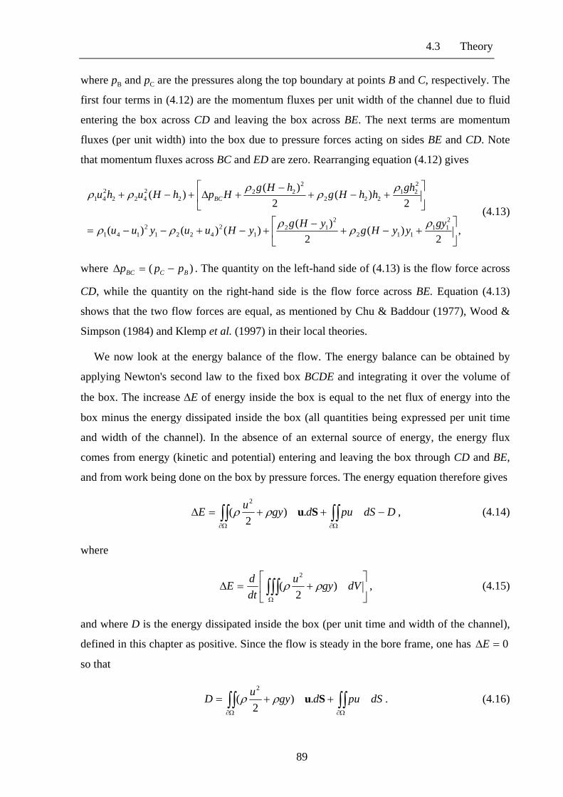
4.3 Theory
where pB and pC are the pressures along the top boundary at points B and C, respectively. The
first four terms in (4.12) are the momentum fluxes per unit width of the channel due to fluid
entering the box across CD and leaving the box across BE. The next terms are momentum
fluxes (per unit width) into the box due to pressure forces acting on sides BE and CD. Note
that momentum fluxes across BC and ED are zero. Rearranging equation (4.12) gives
,2
)(2
)()()()(
2)(
2)()(
211
112
212
12
42212
141
221
222
222
22422
241
⎥⎦
⎤⎢⎣
⎡+−+
−+−+−−=
⎥⎦
⎤⎢⎣
⎡+−+
−+Δ+−+
gyyyHgyHgyHuuyuu
ghhhHghHgHphHuhu BC
ρρρρρ
ρρρρρ (4.13)
where )( BCBC ppp −=Δ . The quantity on the left-hand side of (4.13) is the flow force across
CD, while the quantity on the right-hand side is the flow force across BE. Equation (4.13)
shows that the two flow forces are equal, as mentioned by Chu & Baddour (1977), Wood &
Simpson (1984) and Klemp et al. (1997) in their local theories.
We now look at the energy balance of the flow. The energy balance can be obtained by
applying Newton's second law to the fixed box BCDE and integrating it over the volume of
the box. The increase ΔE of energy inside the box is equal to the net flux of energy into the
box minus the energy dissipated inside the box (all quantities being expressed per unit time
and width of the channel). In the absence of an external source of energy, the energy flux
comes from energy (kinetic and potential) entering and leaving the box through CD and BE,
and from work being done on the box by pressure forces. The energy equation therefore gives
DdSpudgyuE −++=Δ ∫∫∫∫Ω∂Ω∂
Su.)2
(2
ρρ , (4.14)
where
⎥⎦
⎤⎢⎣
⎡+=Δ ∫∫∫
Ω
dVgyudtdE )
2(
2
ρρ , (4.15)
and where D is the energy dissipated inside the box (per unit time and width of the channel),
defined in this chapter as positive. Since the flow is steady in the bore frame, one has 0=ΔE
so that
∫∫∫∫Ω∂Ω∂
++= dSpudgyuD Su.)2
(2
ρρ . (4.16)
89

Chapter 4: Internal bores in lock releases
Note that energy fluxes across BC and ED are zero. Integrating the latter equation over the
surface of the box BCDE, the dissipation inside the box is given by
.)(2
)()()(2
)(
)())((2
)(2
)(
)(2
)(2
)(22
)(
)(2
)()()(2
)(2
)(2
14
21
11411242
21
2
1141424
22
142224
22
2
414
21
142
21
2
24
22
14
22
2
2
114
214
112
42
242
224
24
124
24
2
uuyguuyyHguuyHg
yuupyHuupuhguhhHguhHg
HupuuyguuyHguhguhHg
yuuuuyHuuuuhuuhHuuD
BB
C
−−−−−+−
−
−−−−+−+−+−
+
++−−+−
−+−
+
+−−
−−++
−+−=
ρρρ
ρρρ
ρρρρ
ρρρρ
(4.17)
Using continuity equations (4.7) and (4.8), the last equation reduces to
,)(
2)(
2
2)(
2)('
24
242
2
24
2
24
214
1
24
1242114
hHuuuu
huuuuhuhygHupD BC
−⎥⎦
⎤⎢⎣
⎡ +−+
+⎥⎦
⎤⎢⎣
⎡ −−+−−Δ=
ρρ
ρρρ
(4.18)
where g' is the reduced gravity, which was defined in chapter 3 as
gg1
21 )('ρ
ρρ −= . (4.19)
The energy equation (4.18) can be derived using a different, though equivalent, approach to
that described above. Applying Bernoulli's theorem in the lower layer between D and E, but
introducing a uniform head loss Δ1 to allow for dissipation, one finds
2
)(2
)( 24
111
214
1uppguu
ED ρρρ +−=Δ+− . (4.20)
Similarly, applying Bernoulli's equation in the upper layer between B and C, but introducing a
uniform head loss Δ2 to allow for dissipation, one finds
22
)( 24
222
242
2uguupBC ρρρ =Δ+
++Δ . (4.21)
Assuming a hydrostatic variation of pressure with depth, pressure differences along top
boundary and bottom boundary are related by
)(')( 211 hygppp EDBC −+−=Δ ρ . (4.22)
90

4.3 Theory
Assuming the head loss is uniform in each layer, the energy dissipated in each layer is equal
to the head loss in the layer times the volume flux in the layer. The total energy D dissipated
in the box BCDE (per unit time and width of the channel) is therefore equal to
22421241 )( Δ−+Δ= hHguhguD ρρ . (4.23)
Using (4.20), (4.21) and (4.22) to eliminate Δ1 and Δ1 and BCpΔ , (4.23) reduces to (4.18). This
is not surprising as the total energy dissipated inside the box BCDE is equal to the energy
dissipated in the lower layer plus the energy dissipated in the upper layer.
In order to find an expression for the pressure difference ΔpBC to close the problem, Chu &
Baddour (1977) and Wood & Simpson (1984) followed the analogy with the single-layer
hydraulic flow. They suggested that all the energy loss occurs within the lower layer. This
approach is consistent with Schijf & Schönfeld's (1953) suggestion that for an internal bore,
energy should be conserved within the layer that is relatively accelerated in traversing the
bore, i.e. within the contracting layer. Assuming that energy is conserved in the upper layer,
Bernoulli's theorem can be applied between B and C to give
22
)()(24
2
242
2uuuppp BCBC ρρ −
+=−=Δ . (4.24)
Using (4.7), (4.8) and (4.24), u1, u2 and ΔpBC can be eliminated from the momentum equation
(4.13). This gives Wood & Simpson's expression for the bore speed
2
1
22
22
2222
21
2214
)2()242()1)((
' ⎥⎦
⎤⎢⎣
⎡+−++−
−+=
βαβαβραβαβαρββαβρ
Hgu , (4.25)
where β is the fractional depth of the bore, defined as
Hy1=β . (4.26)
Equation (4.25) relates the speed of the bore to its height. It represents momentum balance
inside the box BCDE.
Using (4.7), (4.8) and (4.24), u1, u2 and ΔpBC can be eliminated from the energy equation
(4.18). This gives the following expression for the dissipation in the lower layer
⎥⎦
⎤⎢⎣
⎡−
−−−+−+−
= 1
24
222
22
221224
25
23 ')1(2
)2()1)(('
)(
'ρ
βββαβρββαραβα
Hgu
Hgu
Hg
D . (4.27)
91

Chapter 4: Internal bores in lock releases
Long before the theories of Chu & Baddour and Wood & Simpson were published, Yih &
Guha (1955) had proposed a different approach to close the problem. They obtained solutions
by evaluating the momentum balance within each layer, approximating the pressure along the
interface by the average of its value far upstream and far downstream. Later authors used a
similar approach to that of Yih & Guha to model internal bores, most notably Houghton &
Isaacson (1970), Long (1970, 1974), Su (1976) and Baines (1984). Wood & Simpson showed
that Yih & Guha's theory predicts bore speeds which are very close to those given by (4.25).
They explained this by showing that Yih & Guha's approach led to a slight energy gain in the
upper layer without associated work being done on it. Yih & Guha's approximation slightly
underestimates the force on the sloping face, resulting in the energy gain. Because the energy
gain is only small, Yih & Guha's theory gives results which are similar to theories that assume
no energy change, like that of Chu & Baddour and Wood & Simpson.
4.3.1.2 Special limits
When the upper layer density tends to zero, the above problem tends to that of a free surface
bore. In the free surface limit, the bore speed given in (4.25) tends to
2
24
2)(
αβα +
=gHu , (4.28)
and the dissipation given in (4.27) tends to
⎥⎦
⎤⎢⎣
⎡−
+−= 1
2)()( 2
42
2224
25
23
1gHu
gHu
Hg
Dβ
βααβα
ρ. (4.29)
Combining (4.28) with (4.29), one obtains
gH
u
Hg
Dβ
αβ
ρ 4)( 3
24
25
23
1
−= . (4.30)
Energy is therefore still dissipated in the lower layer in the free surface limit. This is
consistent with the fact that any dissipation when ρ2 tends to zero can only occur in the lower
layer.
As mentioned in chapter 1, we are mainly interested in situations where density differences
are relatively small. The Boussinesq approximation can therefore be invoked, where density
92

4.3 Theory
differences are neglected, except when coupled with gravity. In the Boussinesq limit, the bore
speed (4.25) in Wood & Simpson's theory reduces to
)23(
)1)((' 22
2
224
αβαβββαβ
+−−+
=Hg
u , (4.31)
When βα /2 tends to one, the speed of the bore reduces to the linear long-wave limit (cf.
Turner 1973, p. 18)
)1('4 ββ −=Hg
u , (4.32)
as expected. On the other hand, in the gravity current limit where βα /2 tends to zero, the
bore speed tends to
)1('4 β−=Hg
u , (4.33)
which differs from Benjamin's expression (3.31). The bore speed tends to one in the limit
where the channel depth becomes large, i.e. where β tends to zero. As mentioned by Klemp et
al. (1997), and as described by Rottman & Simpson (1983), this behaviour is not observed in
laboratory experiments. Indeed, the speed of a gravity current is observed to tend to zero,
rather than one, as its depth becomes shallow with respect to the channel depth.
Under the Boussinesq approximation, the energy equation (4.27) reduces to
⎥⎦
⎤⎢⎣
⎡−
−−−+−+−
= 1')1(2
)2()1)(('
)(
'ˆ
24
222
222224
25
23 Hg
uHg
u
Hg
Dββ
βαβββααβα
ρ, (4.34)
where 12ˆ ρρρ ≈= . Combining (4.31) with (4.34), one obtains
)23(2
)21()(''ˆ 22
2
3224
25
23 αβαββ
βαβα
ρ +−−−
=Hg
u
Hg
D (4.35)
Putting in the last equation, one finds that 0=D 5.0=β or 2αβ = in the absence of
dissipation. These are the local energy-conserving solutions for internal bores. They show
that, in the only non-trivial case, the bore must occupy half the space between the two
boundaries if energy is to be conserved and the flow is to be steady.
93

Chapter 4: Internal bores in lock releases
Equation (4.35) shows that D is always positive for β between α2 and 0.5 in the local
analysis. In general, dissipation must therefore occur in order to have a steady state. Wood &
Simpson argued that this dissipation, in the absence of bottom friction, occurs in the lighter
fluid through downstream waves for undular bores, or through mixing for strong bores.
4.3.1.3 Comparison with experiments
Wood & Simpson (1984), Baines (1984) and Rottman & Simpson (1989) performed some
laboratory experiments to study internal bores in the laboratory. As mentioned by Klemp et
al. (1997), these experiments agree with the classical theories of Yih & Guha and Wood &
Simpson only for weak bores, when β /α2 is smaller than about 2.3. When β /α2 is greater than
about 2.3 however, the classical theories overestimate the speeds measured in experiments
(cf. Klemp et al. 1997, figure 3). Wood & Simpson argued that the discrepancy with their
theory is due to the turbulent mixing that occurs behind the front of the bore when β /α2 is
greater than about 2.3.
As explained in §4.2, internal bores in the above-mentioned experiments differ from the
lock release problem considered in this chapter. The internal bores were created in most of
these experiments by towing a solid obstacle of finite horizontal extent through a two-layer
stratification. The latter problem is quite different from that of a lock release, which is
considered in this chapter. By towing an obstacle, some external energy and momentum are
indeed continually supplied to the system to keep the obstacle speed constant. The above
experiments may therefore not be appropriate for comparison in this chapter. As a result,
some new, lock-release experiments were performed during this thesis. These new
experiments were described in §4.2. The positions in parameter space of all new internal bore
experiments performed were shown in figure 4.3. The Froude number in these new
experiments is defined as
)(' 21
1
hhguF
+= , (4.36)
and was measured in each experiment. The measurements are shown in table 4.1, where they
are compared with Wood & Simpson's predictions. Note that since Wood & Simpson's theory
assumes a steady state, it does not depend on the initial state before release. Their Froude
number predictions therefore do not depend on α1, but on measuring the bore height y1.
94

4.3 Theory
Expt α1 α1 Fa Fb Fc Fexpt B1 1 0,13 0,39 ± 0.01 0,47 ± 0.01 0,43 ± 0.02 0,47 ± 0.015
B2 0,85 0,10 0,50 ± 0.01 0,56 ± 0.01 0,54 ± 0.01 0,48 ± 0.015
B3 0,69 0,10 0,60 ± 0.01 0,62 ± 0.01 0,62 ± 0.01 0,55 ± 0.015
B4 0,52 0,10 0,69 ± 0.01 0,63 ± 0.03 0,69 ± 0.02 0,58 ± 0.02
B5 0,35 0,10 0,79 ± 0.02 0,65 ± 0.05 0,72 ± 0.02 0,60 ± 0.02
B6 0,25 0,10 0,84 ± 0.04 0,65 ± 0.07 0,75 ± 0.05 0,59 ± 0.025
B7 1 0,25 0,34 ± 0.02 0,39 ± 0.01 0,38 ± 0.01 0,42 ± 0.015
B8 0,79 0,25 0,48 ± 0.01 0,50 ± 0.01 0,49 ± 0.01 0,46 ± 0.015
B9 0,57 0,25 0,57 ± 0.01 0,55 ± 0.01 0,57 ± 0.01 0,50 ± 0.015
B10 0,41 0,27 0,61 ± 0.01 0,56 ± 0.01 0,59 ± 0.01 0,53 ± 0.015
B11 0,55 0,40 0,51 ± 0.01 0,51 ± 0.02 0,51 ± 0.02 0,47 ± 0.035
Table 4.1. Wood & Simpson's predictions of front speed based on three heights: the height ha at the
head (Fa), the height hb immediately behind the head (Fb), and the height hc at the lock position (Fc).
The predictions are compared with front speeds Fexpt measured in lock-release experiments presented
in figure 3. Note that all front speeds are non-dimensionalised with )(' 21 hhg + .
As for gravity currents, predictions of Froude numbers can vary substantially, depending
on where the bore height is measured. Three Froude numbers Fa , Fb and Fc are calculated
from Wood & Simpson's relation (4.31) for each experiment, based on the heights ha at the
top of the bore head, the height hb immediately behind the bore head, and the height hc
downstream at the lock position, respectively. Froude numbers based on ha can be lower than
those based on hb by up to a factor of two, causing a large difference in Froude number,
depending on which height measurement is used.1 Wood & Simpson's predictions are
compared with direct measurements of the Froude number in experiments. As can be seen
from table 4.1, predictions based on hb are in reasonable agreement with direct measurements
of the speed across the whole parameter space. Predictions based on ha agree with
1 Note that for undular bores, Wood & Simpson (1984), Baines (1984) and Rottman & Simpson (1989) in
their towed obstacle experiments based their Froude numbers on the average depth behind the front. For turbulent bores however, they based their measurements on the depth of the unmixed fluid immediately behind the head.
95

Chapter 4: Internal bores in lock releases
experiments when the bore height is close to half the channel depth or when the bore strength
is close to one, i.e. near the local energy-conserving solutions. However, for stronger and
shallower bores (cf. the bottom left region of figure 4.3), Froude numbers based on the
heights at the head diverge significantly from measurements. The largest discrepancies are
observed in the limit of very strong, shallow bores (cf. experiments B4, B5 and B6), when α1
and α2 /α1 are both low. In the gravity current limit where α1 and α2 /α1 both tend to zero,
Wood & Simpson's predictions do not tend to Benjamin's prediction, as shown in §4.3.1.1.
Note that Wood & Simpson defined the height y1 used in (4.31) as the interface height far
downstream. The flow downstream is assumed to become uniform so that Bernoulli's theorem
applies. Measuring the bore height immediately behind its front head may therefore not be
appropriate. A better choice in a lock release may be the depth of dense fluid at the lock
position, which lies further downstream. The interface near the lock position becomes indeed
more and more horizontal as the bore and disturbance advance (cf. §4.2). As seen in table 4.1,
measurements based on the height at the lock position suggest that Wood & Simpson's Froude
number equation (4.31) may not be valid in that case for stronger and shallower bores. The
validity of the local theory is discussed further in §4.4.
4.3.2 Local theory : energy conservation in the lower layer
Klemp et al.'s (1997) local analysis of internal bores is presented in §4.3.1.1. Some special
limits are then considered in §4.3.2.2. Finally, Klemp et al.'s theory is compared with
experiments in §4.3.2.3.
4.3.2.1 Analysis
To avoid the unrealistic limit of Wood & Simpson's theory in the gravity current limit, Klemp
et al. (1997) proposed that energy loss occurs in the upper layer. Assuming that energy is
conserved in the lower layer, Klemp et al. applied Bernoulli's theorem along DE so that
22)()(
24
1
214
1uuupp ED ρρ −
−=− , (4.37)
96

4.3 Theory
where pD and pE are the pressures along the bottom boundary at point D and E, respectively.
Combining (4.22) with (4.37), the pressure difference along the top boundary is given by
)('22
)(211
24
1
214
1 hyguuupBC −+−−
=Δ ρρρ . (4.38)
Using (4.7), (4.8) and (4.38), u1, u2 and ΔpBC can be eliminated from the momentum equation
(4.13) to yield
[ ]2
1
22
2221
22
14
)1(2)2)(1()2)(1(
' ⎭⎬⎫
⎩⎨⎧
−+−+−−−−
=αβρβαβαβρ
βαββρHg
u , (4.39)
Equation (4.39) relates the speed of the bore to its height. It represents momentum balance
inside the box BCDE.
Similarly, u1, u2 and ΔpBC can be eliminated from the energy equation (4.18) to yield
⎥⎦
⎤⎢⎣
⎡−
−−+−+−
−−=
Hgu
Hgu
Hg
D')1(2
)2()1)(('
))(1(
'
24
222
22
221
1224
25
23 ββ
βαβρββαρραβα . (4.40)
4.3.2.3 Special limits
In the free-surface limit where the upper layer density tends to zero, the bore speed (4.39) in
Klemp et al.'s theory tends to
)2(
)2(
22
22
4
βαβαβαβ
−+−−
=gHu , (4.41)
and the dissipation in the upper layer given in (4.40) tends to
⎥⎦
⎤⎢⎣
⎡ +−
−−=
gHu
gHu
Hg
D 24
22224
25
23
12
)(1))(1(β
βααβα
ρ. (4.42)
Combining (4.41) with (4.42), one obtains
)2(2
))(1(
22
3224
25
23
1βαβα
αβα
ρ −+−−
=gHu
Hg
D . (4.43)
Energy is therefore still dissipated in the upper layer in the free surface limit. This result is
inconsistent with the fact that the energy can only be dissipated within the lower layer when
ρ2 tends to zero. Klemp et al. realised the problem, and suggested that the nature of the energy
97

Chapter 4: Internal bores in lock releases
loss within a Boussinesq internal bore may differ from that in a free surface bore owing to
differing vorticity characteristics within the bore. To show this, they derived a theory of
localised mixing where energy dissipation is allowed in each of the two layers, but is confined
to the vicinity of the interface between the two layers. They suggested that free surface bores
develop a circulation that causes their leading edge to curl forward, producing turbulent
eddies that penetrate back into the lower layer. This circulation creates a velocity profile that
decreases with height. Based on their theory of localised mixing, they showed that energy
should in this case be lost mostly in the lower layer, in agreement with the classical theories
of Yih & Guha (1955) and Wood & Simpson (1984). On the other hand, for internal bores
forming in Boussinesq fluids, strong baroclinic vorticity generation in the head region occurs
in the opposite direction to that arising in free surface bores. As a result, the flow near the
interface is swept to the rear, so that turbulence forms through Kelvin-Helmholtz instability
behind the head. In this situation, flow beneath the interface is accelerated by shear stresses
owing to the faster moving fluid aloft. Based on their theory of localised mixing, Klemp et al.
showed in that case that energy should be lost mostly in the upper layer, and gained slightly in
the upper layer. They concluded that, for Boussinesq internal bores, the assumption of energy
conservation in the lower layer is a better approximation than the reverse assumption of
energy conservation in the upper layer. As a result, Klemp et al. applied their theory only to
Boussinesq fluids.
Under the Boussinesq approximation, the momentum equation (4.39) reduces to
)3()2)(1(
' 222
22
4
βαβαββαββ
++−−−−
=Hg
u . (4.44)
When βα /2 tends to one, i.e. for weak bores, the speed of the bore reduces to the linear long-
wave limit (cf. Turner 1973, p. 18)
)1('4 ββ −=Hg
u , (4.45)
as expected. Moreover, in the gravity current limit where βα /2 tends to zero, the bore speed
tends to Benjamin's expression (3.31) for the gravity current speed, in contrast to Wood &
Simpson's theory.
Under the Boussinesq approximation, the energy equation (4.40) reduces to
98

4.3 Theory
⎥⎦
⎤⎢⎣
⎡−
−−+−+−
−−=
Hgu
Hgu
Hg
D')1(2
)2()1)((1'
))(1(
'ˆ
24
222
222224
25
23 ββ
βαβββααβα
ρ (4.46)
Combining (4.44) with (4.46), one obtains
)3)(1(2
)21())(1(''ˆ 22
2
3224
25
23 βαβαββ
βαβα
ρ ++−−−−−
=Hg
u
Hg
D . (4.47)
Note that (4.47) reduces to Benjamin's (1968) gravity current expression (3.23) in chapter 3
for the dissipation when α2 tends to zero. Putting 0=D in the last equation, one finds that
5.0=β or 2αβ = in the absence of dissipation. These are the local energy-conserving
solutions, which are the same in Klemp et al.'s theory and in Wood & Simpson's theory, as
expected. They show that, in the only non-trivial case, the bore must occupy half the space
between the two boundaries if momentum and energy are to be conserved and the flow is to
be steady.
Equation (4.47) shows that D is always positive for 5.02 ≤≤ βα in the local analysis. In
general, dissipation must therefore occur in order to have a steady state. Klemp et al. argued
that this dissipation, in the absence of bottom friction, occurs in the lighter fluid through
mixing and viscous dissipation.
4.3.2.3 Comparison with experiments
Klemp et al. compared their theory with the laboratory experiments of Wood & Simpson
(1984), Baines (1984) and Rottman & Simpson (1989). In the comparison, they based their
Froude numbers on the height of the bore behind the bore head. The experiments were found
to be in better agreement with Klemp et al.'s local theory (cf. Klemp et al. 1997, figure 3)
than with Wood & Simpson's theory. However, the internal bores in most of the above
experiments were created by towing a solid obstacle of finite horizontal extent through a two-
layer stratification. As mentioned in §4.3.1.3, the latter problem is quite different from that of
a lock release, which is considered in this chapter. The above experiments may therefore not
be appropriate for comparison in this chapter. In this section, Klemp et al.'s theory is therefore
compared to the new, lock-release experiments described in §4.2. The positions in parameter
space of all the new internal bore experiments performed were shown in figure 4.3. The
Froude number, defined in (4.36), was measured in each of these experiments. As in §4.3.1.3,
three Froude numbers, Fa , Fb and Fc , are calculated from Klemp et al.'s relation (4.44) for
99

Chapter 4: Internal bores in lock releases
each experiment. They are based respectively on the height ha at the top of the bore head, the
height hb immediately behind the bore head, and the height hc downstream at the lock
position. The measurements are shown in table 4.2, where they are compared with Klemp et
al.'s predictions. Note that, as in Wood & Simpson's theory, Klemp et al.'s theory assumes a
steady state and therefore does not depend on the initial state before release.
Expt α1 α1 Fa Fb Fc Fexpt B1 1 0,13 0,43 ± 0.01 0,47 ± 0.01 0,45 ± 0.02 0,47 ± 0.015
B2 0,85 0,10 0,51 ± 0.01 0,53 ± 0.01 0,52 ± 0.01 0,48 ± 0.015
B3 0,69 0,10 0,58 ± 0.01 0,58 ± 0.01 0,58 ± 0.01 0,55 ± 0.015
B4 0,52 0,10 0,66 ± 0.01 0,60 ± 0.03 0,64 ± 0.02 0,58 ± 0.02
B5 0,35 0,10 0,74 ± 0.02 0,63 ± 0.05 0,68 ± 0.02 0,60 ± 0.02
B6 0,25 0,10 0,79 ± 0.04 0,64 ± 0.07 0,74 ± 0.05 0,59 ± 0.025
B7 1 0,25 0,38 ± 0.02 0,41 ± 0.01 0,41 ± 0.01 0,42 ± 0.015
B8 0,79 0,25 0,48 ± 0.01 0,50 ± 0.01 0,49 ± 0.01 0,46 ± 0.015
B9 0,57 0,25 0,56 ± 0.01 0,54 ± 0.01 0,56 ± 0.01 0,50 ± 0.015
B10 0,41 0,27 0,60 ± 0.01 0,56 ± 0.01 0,59 ± 0.01 0,53 ± 0.015
B11 0,55 0,40 0,51 ± 0.01 0,51 ± 0.02 0,51 ± 0.02 0,47 ± 0.035
Table 4.2. Klemp et al.'s predictions of front speed based on three heights: the height ha at the head
(Fa), the height hb immediately behind the head (Fb), and the height hc at the lock position (Fc). The
predictions are compared with front speeds Fexpt measured in lock-release experiments presented in
figure 3. Note that all front speeds are non-dimensionalised with )(' 21 hhg + .
As can be seen from table 4.2, all predicted Froude numbers are in good agreement with
experiments when the bore height is close to half the channel depth or when the bore strength
is close to one, i.e. near the energy-conserving solutions. However, for stronger and shallower
bores (cf. experiments B4, B5 and B6), only predictions based on the height measured
immediately behind the head agree with measurements. Froude numbers based on the heights
at the head or at the lock position diverge significantly from local theory in this region (cf. the
bottom left region of figure 4.3). The largest discrepancies are observed in the limit of very
strong, shallow bores (α2 tending to zero and α1 lower than about 0.5). In this limit, the bores
tend to gravity currents and Klemp et al.'s theory tends to Benjamin's (1968) theory.
100

4.3 Theory
Benjamin's predictions based on the height at the lock position were shown in chapter 3 to
diverge from lock-release experiments by up to about 40 percent for shallower gravity
currents.
4.3.3 Shallow-water theory
4.3.3.1 Energy conservation in the upper layer
As for uniform gravity currents, two-layer shallow-water theory can be used to solve for the
initial-value problem presented in §4.2. As in the local analyses of §4.3.1, velocities in each
layer are assumed to be independent of vertical position. The equations of motion and
variables in each layer are the same as in §3.3.2. The flow is assumed to be inviscid,
incompressible and immiscible. It is also assumed to be mainly horizontal. Clearly, the latter
assumption is not valid in the very initial moments of the release, when vertical accelerations
are not negligible. However, as described in §4.2, the flow rapidly accelerates to a steady
speed. The assumption should therefore be valid during most of the initial phase of a lock
release.
With the Boussinesq approximation, the solution to the equations of motion was shown in
§3.3.2 to be equivalent to the solution of the ordinary differential equations
( ) 021dd
11
11 =±+−− λua
yuy , (4.48)
where the characteristic speeds ±λ were given by
[ ]21
)1(')1( 122
11 bygauau −+±−=±λ , (4.49)
and where a and b were defined as
)1( β
β−
=a , (4.50)
( ) 221 1'
−−+= ββHg
ub . (4.51)
If the backward disturbance is a rarefaction wave, the velocity of the dense fluid is zero at the
leading edge of the disturbance, so that
101

Chapter 4: Internal bores in lock releases
01 =u when 11 hy = . (4.52)
Following the description in §4.2, the latter condition should be valid when α1 is lower than a
value that varies between about 0.5 and 0.75, depending on α2.
(a)
Expt α1 α1 hf ha hb B1 1 0,13 0.61 0,54 ± 0.03 0,44 ± 0.03
B2 0,85 0,10 0.48 0,55 ± 0.03 0,44 ± 0.03
B3 0,69 0,10 0.46 0,56 ± 0.04 0,45 ± 0.04
B4 0,52 0,10 0.45 0,66 ± 0.05 0,38 ± 0.05
B5 0,35 0,10 0.46 0,62 ± 0.06 0,40 ± 0.06
B6 0,25 0,10 0.48 0,67 ± 0.08 0,42 ± 0.08
B7 1 0,25 0.61 0,54 ± 0.02 0,49 ± 0.02
B8 0,79 0,25 0.50 0,51 ± 0.03 0,42 ± 0.08
B9 0,57 0,25 0.49 0,53 ± 0.04 0,42 ± 0.04
B10 0,41 0,27 0.50 0,56 ± 0.04 0,43 ± 0.04
B11 0,55 0,40 0.50 0,53 ± 0.03 0,43 ± 0.03
Table 4.3. (a) Front heights hf predicted by shallow-water theory using Wood & Simpson's front
condition. These predictions are compared with front heights measured in lock-release experiments
at the top of the front head (ha) and immediately behind the front (hb). All front heights are non-
dimensionalised with (h1+h2). (b). Front speeds Ftheory predicted by shallow-water theory using
Wood & Simpson's front condition. These predictions are compared with front speeds Fexpt
measured in lock-release experiments presented in figure 3. All front speeds are non-dimensionalised
with )(' 21 hhg + .
(b)
Expt α1 α1 Ftheory Fexpt B1 1 0,13 0.32 0,47 ± 0.015
B2 0,85 0,10 0.54 0,48 ± 0.015
B3 0,69 0,10 0.62 0,55 ± 0.015
B4 0,52 0,10 0.68 0,58 ± 0.02
102

4.3 Theory
B5 0,35 0,10 0.70 0,60 ± 0.02
B6 0,25 0,10 0.71 0,59 ± 0.025
B7 1 0,25 0.27 0,42 ± 0.015
B8 0,79 0,25 0.48 0,46 ± 0.015
B9 0,57 0,25 0.56 0,50 ± 0.015
B10 0,41 0,27 0.59 0,53 ± 0.015
B11 0,55 0,40 0.51 0,47 ± 0.035
Table 4.3. (continued)
A condition must be specified at the front of the bore to close the problem. Using +λ in
(4.48) and (4.49), one can integrate the characteristic equation in the direction of decreasing
y1, subject to the initial condition (4.52), until a specified front condition is satisfied. This
allows us to find the front speed and height of bores as a function of initial fractional depths
α1 and α2.
Table 4.3a compares the predicted front heights with heights measured at the top of the
front head (ha) and immediately behind the head (hb). As shown in the previous section, ha
and hb can differ by a factor of up to two. A comparison with theory is therefore difficult.
Nevertheless, assuming that the front height lies between ha and hb, predictions based on
Wood & Simpson's front condition seem consistent with the experiments performed.
Table 4.3b compares the front speeds predictions based on Wood & Simpson's front
condition (4.31) with internal bore lock-release experiments. As can be seen, predictions
based on Wood & Simpson's front condition do not agree in general with experiments. The
discrepancy reaches about 35 percent in some experiments (cf. experiments B1 and B7).
4.3.3.2 Energy conservation in the lower layer
Table 4.4a compares front height predictions based on Klemp et al.'s front condition (4.44)
with heights measured at the top of the front head and immediately behind it. As in the
previous section, a comparison with theory is difficult due to the large possible difference
between ha and hb. Nevertheless, assuming that the front height lies between ha and hb,
predictions based on Klemp et al.'s Froude number condition seem consistent with the
experiments performed.
103

Chapter 4: Internal bores in lock releases
Table 4.4b compares the front speed obtained from shallow-water theory based on Klemp
et al.'s Froude number condition (4.44) with internal bore lock-release experiments. As can be
seen, the agreement is generally good, especially near the energy-conserving solutions (near
the half-depth solution or for very weak bores). However, as for Froude numbers in §4.3.2.3,
experiments diverge from local theory for stronger and shallower bores (γ larger than about
two and α1 greater than about one). The discrepancy is largest near the gravity current limit,
where the local theory was found in chapter 3 to overestimate the front speed by up to about
20 percent.
(a)
Expt α1 α1 hf ha hb B1 1 0,13 0.55 0,54 ± 0.03 0,44 ± 0.03
B2 0,85 0,10 0.49 0,55 ± 0.03 0,44 ± 0.03
B3 0,69 0,10 0.47 0,56 ± 0.04 0,45 ± 0.04
B4 0,52 0,10 0.47 0,66 ± 0.05 0,38 ± 0.05
B5 0,35 0,10 0.47 0,62 ± 0.06 0,40 ± 0.06
B6 0,25 0,10 0.48 0,67 ± 0.08 0,42 ± 0.08
B7 1 0,25 0.56 0,54 ± 0.02 0,49 ± 0.02
B8 0,79 0,25 0.50 0,51 ± 0.03 0,42 ± 0.08
B9 0,57 0,25 0.49 0,53 ± 0.04 0,42 ± 0.04
B10 0,41 0,27 0.50 0,56 ± 0.04 0,43 ± 0.04
B11 0,55 0,40 0.50 0,53 ± 0.03 0,43 ± 0.03
Table 4.4. (see caption on the oppposite page )
Klemp et al.(1997) performed numerical simulations of internal bore lock releases in a
limited portion of the parameter space. Their simulations agree with shallow-water theory
based on their Froude number condition. However, their internal bore simulations
significantly overestimate front speeds measured near the limit of shallow gravity current. In
the latter limit, their simulations overestimate the front speeds of gravity current measured in
experiments by Rottman & Simpson (1983) and the new ones reported in this thesis by up to
about 20 percent. A similar discrepancy occurred in their gravity current numerical
simulations (cf. Klemp et al. 1994), as discussed in chapter 3. For the same reasons as those
104

4.3 Theory
discussed in §3.3.2, mixing and bottom friction are unlikely to account for such large
discrepancies at the Reynolds numbers considered in this thesis, which are all higher than
1500. A new theory for the lock release of internal bores is therefore presented in the next
section.
(b)
Expt α1 α1 Ftheory Fexpt B1 1 0,13 0.43 0,47 ± 0.015
B2 0,85 0,10 0.52 0,48 ± 0.015
B3 0,69 0,10 0.58 0,55 ± 0.015
B4 0,52 0,10 0.63 0,58 ± 0.02
B5 0,35 0,10 0.67 0,60 ± 0.02
B6 0,25 0,10 0.69 0,59 ± 0.025
B7 1 0,25 0.37 0,42 ± 0.015
B8 0,79 0,25 0.48 0,46 ± 0.015
B9 0,57 0,25 0.56 0,50 ± 0.015
B10 0,41 0,27 0.59 0,53 ± 0.015
B11 0,55 0,40 0.51 0,47 ± 0.035
Table 4.4. (a) Front heights hf predicted by shallow-water theory using Klemp et al.'s front condition.
These predictions are compared with front heights measured in lock-release experiments at the top of
the front head (ha) and immediately behind the front (hb). Front heights are non-dimensionalised with
(h1+h2). (b) Front speeds Ftheory predicted by shallow-water theory using Klemp et al.'s front
condition. These predictions are compared with front speeds Fexpt measured in lock-release
experiments presented in figure 3. All front speeds are non-dimensionalised with )(' 21 hhg + .
4.3.4 Global theory
In light of the discrepancies that exist between the local analyses and experiments in a
significant portion of the parameter space, a new theory is presented in this section for the
lock release of internal bores. The new theory is similar in some ways to Klemp et al.'s (1997)
theory, but applies conservation of mass, momentum and energy globally rather than locally.
It is therefore similar in some respect to shallow-water theory in that it considers both sides of
105

Chapter 4: Internal bores in lock releases
the lock release. The new theory nevertheless distinguishes itself from shallow-water theory
by introducing some approximations in order to find analytical rather than numerical
solutions. The analysis of the model is presented in §4.3.3.1, then compared with lock-release
experiments in §4.3.3.2. In §4.3.3.3, the new theory is compared with shallow-water theory.
4.3.4.1 Analysis
The lock release problem was described in §4.2, where densities, velocities and initial heights
were defined (cf. figure 4.1). In the global theory, fluid is assumed to be inviscid, irrotational
and immiscible. Layers are uniform and velocities are purely horizontal. The shape of the
interface is approximated by a horizontal middle section of height y1 and two advancing
fronts. The two fronts are assumed to have a constant shape in time. As in the local analyses
presented in §4.3.1 and §4.3.2, the exact shape of the fronts does not matter as long as it
remains steady. The fronts move at constant speeds u3 towards the right and u4 towards the
left. A similar approximation was used in the local analyses, where the interface was assumed
to become horizontal far downstream of the bore. As described in §4.2, the backward
disturbance is in general a rarefaction wave rather than a front of constant shape. The
interface shape is therefore only an approximation, aimed at simplifying calculations in the
following theory. The validity of the approximation will be examined in more detail in §4.4.
The situations in the bore frame and in the disturbance frame after the release were depicted
in figures 4.2a and 4.2b, where bore and disturbance fronts, respectively, are at rest. Applying
conservation of mass in each layer across the bore front and disturbance front, one obtains the
three independent equations
11323 )( yuuhu −= , (4.53)
))(()( 13223 yHuuhHu −+=− , (4.54)
14114 )( yuuhu += . (4.55)
The latter equations yield the continuity equations
)( 1
112 yH
yuu−
= , (4.56)
)( 21
113 hy
yuu−
= , (4.57)
106
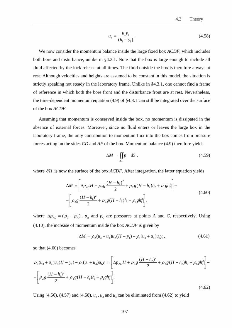
4.3 Theory
)( 11
114 yh
yuu−
= . (4.58)
We now consider the momentum balance inside the large fixed box ACDF, which includes
both bore and disturbance, unlike in §4.3.1. Note that the box is large enough to include all
fluid affected by the lock release at all times. The fluid outside the box is therefore always at
rest. Although velocities and heights are assumed to be constant in this model, the situation is
strictly speaking not steady in the laboratory frame. Unlike in §4.3.1, one cannot find a frame
of reference in which both the bore front and the disturbance front are at rest. Nevertheless,
the time-dependent momentum equation (4.9) of §4.3.1 can still be integrated over the surface
of the box ACDF.
Assuming that momentum is conserved inside the box, no momentum is dissipated in the
absence of external forces. Moreover, since no fluid enters or leaves the large box in the
laboratory frame, the only contribution to momentum flux into the box comes from pressure
forces acting on the sides CD and AF of the box. Momentum balance (4.9) therefore yields
, (4.59) ∫∫Ω∂
=Δ dSpM
where is now the surface of the box ACDF. After integration, the latter equation yields Ω∂
,)(2
)(
)(2
)(
211112
21
2
221222
22
2
⎥⎦
⎤⎢⎣
⎡+−+
−−
−⎥⎦
⎤⎢⎣
⎡+−+
−+Δ=Δ
ghhhHghHg
ghhhHghHgHpM AC
ρρρ
ρρρ (4.60)
where )( ACAC ppp −=Δ , pA and pC are pressures at points A and C, respectively. Using
(4.10), the increase of momentum inside the box ACDF is given by
1143112432 )()()( yuuuyHuuuM +−−+=Δ ρρ , (4.61)
so that (4.60) becomes
,)(2
)(
)(2
)()()()(
211112
21
2
221222
22
21143112432
⎥⎦
⎤⎢⎣
⎡+−+
−−
−⎥⎦
⎤⎢⎣
⎡+−+
−+Δ=+−−+
ghhhHghHg
ghhhHghHgHpyuuuyHuuu AC
ρρρ
ρρρρρ
(4.62)
Using (4.56), (4.57) and (4.58), u2 , u3 and u4 can be eliminated from (4.62) to yield
107

Chapter 4: Internal bores in lock releases
))((
)()(2
)('2111
2121
2121
22
21
2 hyyhhhyuhhgHpAC −−
−−−
−=Δ
ρρρ . (4.63)
As in the global model for gravity currents described in chapter 3, time-dependent Bernoulli's
equation can be applied in the top layer to find the pressure difference between A and C.
Assuming that energy is conserved in the top layer, this gives
C
CA
A tp
tp
∂∂
+=∂
∂+ 2
22
2φρφρ , (4.64)
where φ2 is a velocity potential that must be found, such that
topu=∇ 2φ , (4.65)
where u top is the velocity field inside the top layer. The potential function φ2 is required to be
continuous within the whole layer. Since velocities vary only horizontally within each layer,
the last equation reduces to
x
utop ∂∂
= 2φ , (4.66)
where utop is the velocity function in the top layer, given by
utop = 0 for 4xx ≤ (4.67)
u2 for 34 xxx ≤<
0 for , 3xx >
where x3 and x4 are the positions along the x-axis of the disturbance front and the bore front,
respectively. As before, the x-axis is chosen to have its positive direction towards the left of
figure 4.1b. A possible choice of φ2 , which satisfies (4.66) and (4.67) and is continous for all
x, is given by
φ2 = 0 for 4xx ≤ (4.68)
)( 42 xxu − for 34 xxx ≤≤
)( 432 xxu − for . 3xx ≥
Substituing the latter potential function into (4.64), one obtains
)( 4322 xxupp AC −=− ρ . (4.69)
108

4.3 Theory
Hence, one finds that
)( 4322 uuupAC +=Δ ρ . (4.70)
Note that there is an infinite number of choices for φ2, which all give the same pressure
difference.
Combining (4.56) to (4.58) with (4.63) and (4.70), one obtains the momentum equation
[ ]12112
2121121
)(2)1)()()((
' yyHHgu
ρρββαββαααρ
+−−−−+
= , (4.71)
where α1 = h1 / H, α2 = h2 / H and β = y1 / H as before.
We now look at the energy balance of the flow in the laboratory frame. As in §4.3.1 the
balance is obtained by applying Newton's second law, and integrating over the volume of the
box. This time however, the larger fixed box ACDF is used, rather than the fixed box BCDE.
Since no fluid enters or leaves the box through AF, CD, AC or DF, the energy flux into the
box (including contribution from work due to pressure forces) is zero. Equations (4.14) and
(4.15) therefore yield
⎥⎦
⎤⎢⎣
⎡+−= ∫∫∫
Ω
dVgyudtdD )
2(
2
ρρ . (4.72)
The energy D dissipated inside the box ACDF per unit time and width of the channel is
therefore given by
2
)('2
)(')(2
))((2
21
21
41
22
21
31431
21
1431
22
2yhughyuguuyuuuyHuD −
+−
−+−+−−= ρρρρ .
(4.73)
Assuming that energy is conserved inside the box ACDF, the energy dissipated per unit time
inside the box is zero. Putting D = 0, the energy equation (4.73) therefore reduces to
. (4.74) 0)(')(')())(( 21
2141
22
2131431
211431
222 =−+−−+−+−− yhughyuguuyuuuyHu ρρρρ
Using continuity equations (4.56) to (4.58) to substitute for u2 , u3 and u4, (4.74) reduces to
[ ] 0)1)()((
)1()'(
)()'( 21
2121
1212
11 =
⎭⎬⎫
⎩⎨⎧
−−−+−
−−βαββα
βρβρβρβααHg
u
Hg
u . (4.75)
109

Chapter 4: Internal bores in lock releases
Using the momentum equation (4.71), the energy balance equation (4.75) becomes
02
)(1)()'(
2121
21
11 =⎥⎦
⎤⎢⎣
⎡ +−−
βααβααρ
Hg
u . (4.76)
Thus, in the only non-trivial case, we obtain the solution
2
)( 21 ααβ += . (4.77)
In other words, when momentum and energy conservation is applied to the larger box ACDF,
the bore height is equal to the average h of the initial heights of dense fluid before release.
From (4.71), the speed of the bore, non-dimensionalised with the external scale , is
given by
)( 21 hh +
[ ])()2(2)2(
)(' 212211
211
21
4
ααρααρααρ
++−−−−
=+ hhg
u , (4.78)
Using equations (4.77) and (4.78), the height and speed of an internal bore in a lock release
can be determined given only the initial fractional depth before release. From (4.57), one
finds
43 uu = , (4.79)
so that the speed of the disturbance front in the model is equal to that of the bore front. Note
that the internal bore energy-conserving solution (4.77)-(4.79) tends to the gravity current
energy-conserving solution (3.71)-(3.73) in the limit where 12 /αα tends to zero, as expected.
In contrast to local theories, we just found that applying conservation laws to the lock
release as a whole does not yield a unique solution regardless of initial depths. Instead, a
whole range of solutions 10 ≤≤ β is possible, depending on the initial parameters α1 and α2
before release. This means that dissipation need not be introduced, in contrast to Wood &
Simpson's (1984) theory and Klemp et al.'s (1997) theory. Additional terms on the
disturbance side balance the energy terms on the bore side, so that energy can be conserved
overall. The validity of the energy-conserving solution is discussed further in §4.4.
In the above analysis, we applied Bernoulli's equation in the top layer to get the pressure
difference given in (4.70). The same energy-conserving solution (4.77)-(4.79) is actually
obtained if Bernoulli's equation is applied in the bottom layer. A proof of this result is given
110

4.3 Theory
in appendix A. This result is not surprising as the total energy inside the box ACDF is
necessarily conserved if the energy is conserved within each layer.
4.3.4.2 Special limits
The above energy-conserving solution was derived without using the Boussinesq
approximation. It is therefore theoretically valid for any pair of densities ρ1 and ρ2. We expect
however the above model to break down for non-Boussinesq fluids. The model assumes that
the bore and disturbance sides can be matched by a flat interface in the middle section, where
velocities are horizontal and conditions are uniform. Although laboratory experiments show
that this assumption should be valid for Boussinesq fluids (cf. §4.2), this assumption may be
wrong for non-Boussinesq internal bores, for the same reasons as those explained in §3.3.3.1.
As explained in chapter 1, this thesis focuses on situations where density differences are
relatively small. For the latter reason, and in light of the differences between the model and
non-Boussinesq gravity currents, the rest of this chapter will concentrate on Boussinesq
currents.
Under the Boussinesq approximation, the bore speed (4.78) reduces to
2
)2()('
21
21
4 αα −−=
+ hhgu . (4.80)
and the bore height (4.77) and disturbance speed (4.79) remain unchanged. When the bore
strength 2/αβ tends to one, the speed of the bore reduces to the linear long-wave limit (cf.
Turner 1973, p. 18)
)1('4 ββ −=Hg
u , (4.81)
as expected. Moreover, in the gravity current limit where 12 /αα tends to zero, the latter
Boussinesq solution tends to the global gravity current solution (3.76) of chapter 3, as
required.
4.3.4.3 Comparison with experiments
Table 4.5a compares the height solution (4.77) with measurements in the lock release
experiments. The height y1 was defined in §4.3.3.1 as the height of the interface at the lock
position. Predictions of the new model are therefore compared with measurements at the lock
111

Chapter 4: Internal bores in lock releases
position, where the interface is mainly horizontal. As can be seen, the agreement between the
new model and all experiments performed is good.
(a)
Expt α1 α1 y1 hc B1 1 0,13 0.50 0,50 ± 0.04
B2 0,85 0,10 0.50 0,48 ± 0.03
B3 0,69 0,10 0.50 0,50 ± 0.04
B4 0,52 0,10 0.50 0,48 ± 0.05
B5 0,35 0,10 0.50 0,49 ± 0.04
B6 0,25 0,10 0.50 0,53 ± 0.09
B7 1 0,25 0.50 0,50 ± 0.02
B8 0,79 0,25 0.50 0,48 ± 0.03
B9 0,57 0,25 0.50 0,51 ± 0.04
B10 0,41 0,27 0.50 0,50 ± 0.04
B11 0,55 0,40 0.50 0,49 ± 0.03
Table 4.5. (a) Comparison between bore heights y1 predicted by the new theory and heights hc
measured in lock-release experiments at the lock position. Note that front heights are non-
dimensionalised with (h1+h2). (b) Comparison between front speeds Ftheory predicted by the new
theory and front speeds Fexpt measured in lock-release experiments. Note that all front speeds are
non-dimensionalised with )(' 21 hhg + .
(b)
Expt α1 α1 Ftheory Fexpt B1 1 0,13 0.47 0,47 ± 0.015
B2 0,85 0,10 0.51 0,48 ± 0.015
B3 0,69 0,10 0.55 0,55 ± 0.015
B4 0,52 0,10 0.59 0,58 ± 0.02
B5 0,35 0,10 0.62 0,60 ± 0.02
B6 0,25 0,10 0.64 0,59 ± 0.025
B7 1 0,25 0.43 0,42 ± 0.015
112

4.3 Theory
B8 0,79 0,25 0.49 0,46 ± 0.015
B9 0,57 0,25 0.54 0,50 ± 0.015
B10 0,41 0,27 0.58 0,53 ± 0.015
B11 0,55 0,40 0.51 0,47 ± 0.035
Table 4.5. (continued)
An advantage of the new model is that theoretical bore speeds can be predicted directly
from initial parameters. Predictions do not rely on height measurements, unlike in Klemp et
al.'s theory. Table 4.5b compares the speed solution (4.78) with internal bore experiments.
The agreement is clearly good with all the experiments performed. The small discrepancy is
likely to be due mainly to non-uniform height within the bore, and to a lesser extent to bottom
friction and mixing. The above experiments suggest that these differences should have a
combined effect of less than about ten percent on the bore speed at the Reynolds numbers
considered. This discrepancy agrees with the discussion of §3.3.2 on the effects of bottom
friction and interfacial mixing on the speed of uniform gravity currents.
Note that the new theory can be used to predict whether the released dense fluid forms an
internal bore or a rarefaction wave. An internal bore will be released if its front travels faster
than infinitesimally small long waves on the undisturbed interface ahead, i.e. if
14 λ>u , (4.82)
where the λ1 is the long wave speed ahead of the bore. Using (4.80) and Turner's (1973, p.18)
expression for long wave speed, the latter condition yields
)1(2
)2)((22
2121 αααααα
−>−−+
. (4.83)
After re-arrangement, the latter condition gives
2
)3(2
)(2
)( 212121 αααααα +−>
− , (4.84)
which, since 21 αα ≥ , reduces to
33
2 12
αα −< . (4.85)
113
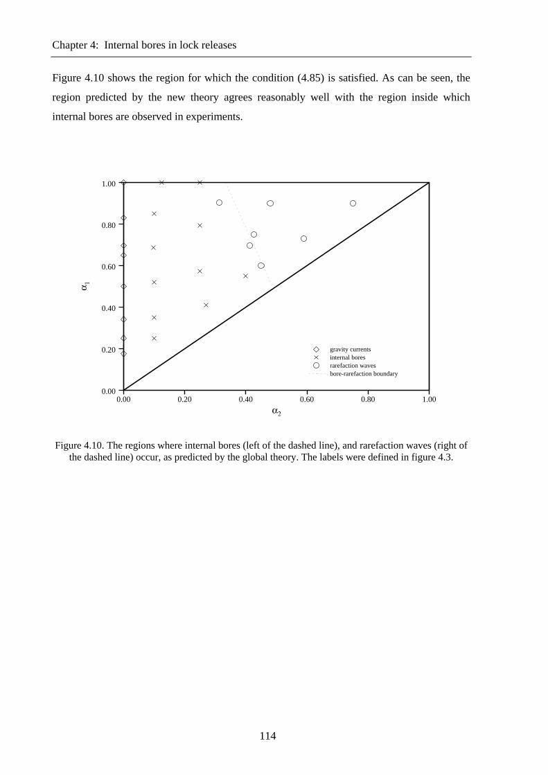
Chapter 4: Internal bores in lock releases
Figure 4.10 shows the region for which the condition (4.85) is satisfied. As can be seen, the
region predicted by the new theory agrees reasonably well with the region inside which
internal bores are observed in experiments.
0.00 0.20 0.40 0.60 0.80 1.000.00
0.20
0.40
0.60
0.80
1.00
gravity currents internal bores rarefaction waves bore-rarefaction boundary
α2
α 1
Figure 4.10. The regions where internal bores (left of the dashed line), and rarefaction waves (right of the dashed line) occur, as predicted by the global theory. The labels were defined in figure 4.3.
114

4.3 Theory
4.3.4.4 Comparison with shallow-water theory
We finish this section by comparing the new model with two-layer shallow-water theory. As
in §4.3.2, the characteristic equation (4.48) can integrated from the leading edge of the
backward disturbance to the front of the bore. A condition must be given at the leading edge
of the disturbance to close the problem. Substituting (4.77) and (4.80) in the momentum
equation (4.71), the speed u1 of the fluid inside the lower layer can be expressed as a function
of β and α2 only, so that
β
βαβ )1()('
22
1
1 −−=
ygu , (4.86)
which reduces to the gravity current condition (3.81) as α2 tends to zero, as expected. Note
that the same condition as above holds at the disturbance jump front because u3= u4. The
condition (4.86) can be used in the analysis of §4.3.2 to predict the height and speed of the
bore in a lock release.
If the leading edge of the disturbance is approximated as a front satisfying the condition
(4.86) as in the global theory, shallow-water theory is automatically consistent with the global
theory. Indeed, disturbance and bore front conditions are the same in the global theory. The
method of integration described in §4.3.2, which leads to a unique solution, is therefore
immediately satisfied. As described in §4.2, the disturbance is a rarefaction wave for α1 lower
than about 0.6. This means that a more realistic condition at the leading edge of the
disturbance would in general be given by (4.52). Equation (4.48) is therefore integrated in the
direction of decreasing y1, subject to the initial condition (4.52), until the front condition
(4.86) is satisfied. This allows us to verify whether the global theory agrees with shallow-
water theory.
Tables 4.6a and 4.6b show bore front heights and speeds as a function of initial fractional
depth, as predicted by shallow-water theory based on Froude condition (4.86). As can be seen
from table 4.6a, the global theory predicts front heights hf that are consistent with experiments
for all initial fractional depths, assuming that the front height lies between the height
measured at the head and that measured immediately behind the head.
As can be seen from table 4.6b, front speeds are very close to the energy-conserving
solution in the global theory. They agree to within about five percent. Moreover, front speeds
predicted by shallow-water theory based on global theory are in good agreement with the
115

Chapter 4: Internal bores in lock releases
lock-release experiments. They agree to within about eight percent. For stronger and
shallower bores (small α1 and large γ), the agreement with measured bore speeds is better
when based on the new theory than on the local theories (cf. tables 4.3b and 4.4b, experiments
B4, B5 and B6).
(a)
Expt α1 α1 hf ha hb B1 1 0,13 0.54 0,54 ± 0.03 0,44 ± 0.03
B2 0,85 0,10 0.50 0,55 ± 0.03 0,44 ± 0.03
B3 0,69 0,10 0.49 0,56 ± 0.04 0,45 ± 0.04
B4 0,52 0,10 0.48 0,66 ± 0.05 0,38 ± 0.05
B5 0,35 0,10 0.49 0,62 ± 0.06 0,40 ± 0.06
B6 0,25 0,10 0.49 0,67 ± 0.08 0,42 ± 0.08
B7 1 0,25 0.55 0,54 ± 0.02 0,49 ± 0.02
B8 0,79 0,25 0.50 0,51 ± 0.03 0,42 ± 0.08
B9 0,57 0,25 0.49 0,53 ± 0.04 0,42 ± 0.04
B10 0,41 0,27 0.50 0,56 ± 0.04 0,43 ± 0.04
B11 0,55 0,40 0.50 0,53 ± 0.03 0,43 ± 0.03
Table 4.6. (a) Front heights hf predicted by shallow-water theory using the new model's front
condition. These predictions are compared with front heights measured in lock-release experiments at
the top of the front head (ha) and immediately behind the front (hb). Note that front heights are non-
dimensionalised with (h1+h2). (b) Front speeds Ftheory predicted by shallow-water theory using the
new model's front condition. These predictions are compared with front speeds Fexpt measured in
lock-release experiments. Note that all front speeds are non-dimensionalised with )(' 21 hhg + .
The good agreement between the new model and shallow-water theory is perhaps not
surprising, as the new model can be seen in some respect as an approximation to shallow-
water theory. Shallow-water theory applies mass and momentum conservation to the lock-
release as whole. The global theory does exactly the same, but uses an approximation for the
shape of the interface to find an analytical rather than numerical solution. The good
116

4.4 Further considerations
agreement between the two theories and lock-release experiments suggests that the
approximation is valid and that the total energy of the system is close to being conserved.
(b)
Expt α1 α1 Ftheory FSWT Fexpt B1 1 0,13 0.47 0.46 0,47 ± 0.015
B2 0,85 0,10 0.51 0.51 0,48 ± 0.015
B3 0,69 0,10 0.55 0.55 0,55 ± 0.015
B4 0,52 0,10 0.59 0.58 0,58 ± 0.02
B5 0,35 0,10 0.62 0.62 0,60 ± 0.02
B6 0,25 0,10 0.64 0.64 0,59 ± 0.025
B7 1 0,25 0.43 0.42 0,42 ± 0.015
B8 0,79 0,25 0.49 0.49 0,46 ± 0.015
B9 0,57 0,25 0.54 0.54 0,50 ± 0.015
B10 0,41 0,27 0.58 0.57 0,53 ± 0.015
B11 0,55 0,40 0.51 0.51 0,46 ± 0.035
Table 4.6. (continued)
4.4 Further considerations
4.4.1 Validity of local theory
As seen in §4.3, local theories agrees in general with experiments and shallow-water theory,
especially near the local energy-conserving solutions ( 5.0=β and 2αβ = ). They diverge
however from experiments for stronger and shallower bores, near the shallow gravity current
limit. In contrast, the global theory agrees well with experiments and shallow-water theory for
all initial fractional depths. This difference suggests that the bore and disturbance sides may
interact in a lock release, so that a local analysis may not always be valid. The local models
assumed that no momentum could be transferred between disturbance and bore sides. They
did not consider the possibility of long waves entering the system. Following shallow-water
117

Chapter 4: Internal bores in lock releases
theory however, long waves can propagate along the interface between the denser and lighter
fluid (cf. §4.3.2). It is believed that these waves can carry momentum from the disturbance
side to the bore side (from the left to the right of figures 4.1b and 4.2b). This transfer modifies
the momentum balance on the bore side, so that the local analyses described in §4.3.1 and
§4.3.2 may not always be appropriate.
As explained in §4.3.1, dissipation must be introduced in Klemp et al's (1997) local
analysis if the flow is to be steady. This dissipation is no longer needed in the new model,
where disturbance and bore sides are both considered in the energy balance. The disturbance
continually releases potential energy as it advances through the fluid. This introduces
additional terms in the energy equation that balance the energy terms on the bore side,
allowing energy to be conserved overall.
From shallow-water theory, long waves travel along the interface with characteristic
speeds ±λ in the laboratory frame given by (cf. equation (4.49))
2
1
211 )1(
)1(')1()21(
⎥⎦
⎤⎢⎣
⎡−
−−±−
−=±
ββββ
ββλ
uHg
u, (4.87)
where +λ denotes characteristic speed from left to right (from disturbance side to current
side), and −λ denotes characteristic speed from right to left (from current side to disturbance
side).
Inserting Klemp et al's momentum equation (4.44) into equation (4.87), one obtains
2
1
222
222
1 )1())(2)(1()3)(1(
)1()21(
⎥⎦
⎤⎢⎣
⎡−
−−−−−
++−−+
−−
=+β
βαββαβ
αββαβββββλ
u. (4.88)
The condition for long waves towards the right to travel faster than the bore front ahead is
given by
3u>+λ . (4.89)
Using (4.86) and (4.88), the latter condition reduces after some algebra to
(4.90) .0)2()73(
)1593()312(522
322
22
32
22
22
32
32
22
42
5
>−+++−+
++−−+−++−
ααβααα
βαααβααβαβ
118
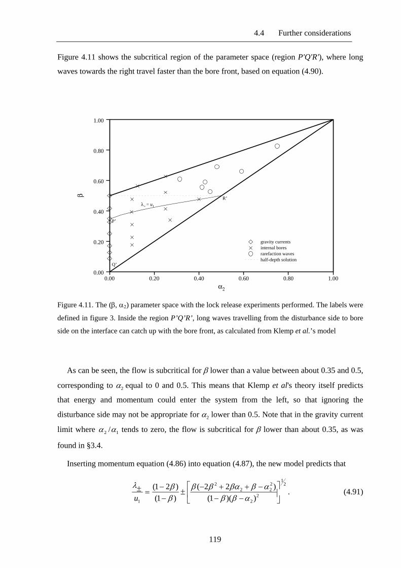
4.4 Further considerations
Figure 4.11 shows the subcritical region of the parameter space (region P'Q'R'), where long
waves towards the right travel faster than the bore front, based on equation (4.90).
0.00 0.20 0.40 0.60 0.80 1.000.00
0.20
0.40
0.60
0.80
1.00
P’
Q’
R’ λ+ = u1
gravity currents internal bores rarefaction waves half-depth solution
α2
β
Figure 4.11. The (β, α2) parameter space with the lock release experiments performed. The labels were
defined in figure 3. Inside the region P’Q’R’, long waves travelling from the disturbance side to bore
side on the interface can catch up with the bore front, as calculated from Klemp et al.’s model
As can be seen, the flow is subcritical for β lower than a value between about 0.35 and 0.5,
corresponding to α2 equal to 0 and 0.5. This means that Klemp et al's theory itself predicts
that energy and momentum could enter the system from the left, so that ignoring the
disturbance side may not be appropriate for α2 lower than 0.5. Note that in the gravity current
limit where 12 /αα tends to zero, the flow is subcritical for β lower than about 0.35, as was
found in §3.4.
Inserting momentum equation (4.86) into equation (4.87), the new model predicts that
2
1
22
222
2
1 ))(1()22(
)1()21(
⎥⎦
⎤⎢⎣
⎡−−
−++−±
−−
=±αββ
αββαββββλ
u. (4.91)
119

Chapter 4: Internal bores in lock releases
From equation (4.91), one can deduce that the two characteristic speeds are always real for
10 2 ≤≤ α and 10 ≤≤ β . Long waves can therefore always travel in both directions in the
laboratory frame. The condition for these long waves towards the right to travel faster than
the bore front ahead is given by
[ ] 0)31()1(3)( 22223
2 >+−+−+− ααβαββαβ , (4.92)
while the condition for long waves towards the left to travel faster than the disturbance front
is given by
[ ] 0)1(3)3(37)( 22223
2 >++−++−− ααβαββαβ . (4.93)
Figure 4.12 shows the regions of parameter space where conditions (4.92) and (4.93) are fulfilled.
0.00 0.20 0.40 0.60 0.80 1.000.00
0.20
0.40
0.60
0.80
1.00
O
P
Q
R
S
T
λ+ = u1
λ- = u1
gravity currents internal bores rarefaction waves half-depth solution
α2
β
Figure 4.12. The (β, α2) parameter space with the lock release experiments performed. The labels were
defined in figure 3. Inside the region PQR, long waves travelling from disturbance side to bore side on
the interface can catch up with the bore front, as calculated using the new model. Inside the region
RST, long waves travelling from bore side to disturbance side on the interface can catch up with the
disturbance front.
120

4.4 Further considerations
Inside region PQR, long waves from right to left never travel faster than the model
disturbance front. However, long waves from left to right always travel faster than the bore
front (except along 2αβ = , where waves and bore front travel at exactly the same speed).
Hence, momentum can be transferred by long waves from disturbance side to bore side.
Klemp et al.'s local model may therefore not apply inside region PQR. Inside region OPRT
however, long waves cannot catch up with either bore front or disturbance front. The two
sides cannot interact and the local analysis should be valid. This explains why the local
analysis agrees well with experiments and shallow-water theory near the local energy-
conserving half-depth solution. Note that the subcritical region PQR predicted by the new
theory agrees well with the subcritical region P'Q'R' predicted by Klemp et al's theory.
Inside region RST, long waves from left to right never travel faster than the bore front, but
long waves from right to left travel faster than the model disturbance front. The two sides are
therefore connected and expected to interact. As can be seen from figure 4.12 however,
rarefaction waves rather than internal bores are found in that region of the parameter space.
Since this chapter concentrates on internal bores, we are not concerned with region RST of the
parameter space.
Long waves are found from (4.91) to travel much faster towards the right than towards the
left for stronger and shallower bores. Moreover, as for gravity currents, long waves from the
disturbance side to the current side travel the fastest for the shallower and stronger bores.
Assuming that momentum flux is proportional to group velocity, these long waves can carry
more momentum for shallower and stronger bores, and the interaction between the
disturbance and bore sides is expected to be strongest for these bores. These results are
consistent with the experiments, for which discrepancies with the local models were shown in
§4.3 to be largest for shallower and stronger bores.
4.4.2 Validity of global energy-conserving solution
In the global theory, the shape of the interface is approximated by a horizontal middle section
and two advancing fronts. In reality, the interface is not perfectly horizontal between the
leading edge of the disturbance and the bore front (cf. figure 4.4c). As described in §4.2, the
leading edge of the disturbance is not a front but a rarefaction wave for α1 lower than about
0.6. The shape of the disturbance changes in that case with time. Despite the approximation
121

Chapter 4: Internal bores in lock releases
used in the new model, it is not claimed in this chapter that the leading edge of the
disturbance is a front. The interface approximation is only aimed at simplifying the time-
dependent analysis of §4.3.3, allowing to derive more easily an expression for the energy
balance. Wood & Simpson and Klemp et al. used a similar approximation to model bores in
their analysis (cf. §4.3.1). The good agreement between the global theory and experiments
suggests that this is a good approximation. Moreover, shallow-water theory, in which
disturbance and interface shapes do change in time, was shown to yield results that were also
in good agreement with both the global theory and experiments (cf. §4.3.2).
We now look more closely at the energy balance in lock releases. One could argue that the
interface approximation might not yield the right energy balance because the shape of the
interface is not quite horizontal and varies with time. The total energy was therefore measured
directly in a number of experiments in order to verify the energy balance. As in §3.4, we
define the energy ratio r in a lock release as
0E
Er T= , (4.94)
where E0 is the initial potential energy inside a chosen fixed box before the release and ET is
the total energy (potential plus kinetic) inside the same box after release. In the global theory,
energy is assumed to be conserved overall so that ET = E0 and 1=r inside a box that contains
all fluid affected by the lock release.
As in §3.4, the energy ratio r was measured in a number of experiments, during the initial
phase of the releases. Measurements were taken before the backward disturbance reflected on
the endwall. For initial depth ratios 21 /αα equal to about 1.5, 2.3 and 4 (experiments B10, B9
and B7, respectively), the energy ratio was measured to be equal to 0.95 ± 0.07, 0.95 ± 0.05
and 0.96 ± 0.05, respectively. These values are all close to one, so that energy is close to
being overall conserved in these experiments. These measurements justify the use of energy
conservation and of the interface approximation in the global theory.
122

4.5 Summary
4.5 Summary
This chapter studied internal bores during the initial stages of a lock release. In a lock release,
a disturbance is always associated with the bore and travels in the opposite direction. When
Wood & Simpson's (1984) theory or Klemp et al.'s (1997) were applied to lock releases, their
analysis could only model the bore side. It was found from these theories that dissipation
must occur in general. The local theories presented some significant discrepancies with
experiments, and with two-layer shallow-water theory, for stronger and shallower bores.
Interfacial mixing is thought to be unlikely to account for these discrepancies. Moreover,
bottom friction is negligible at the Reynolds numbers considered. A new theory was therefore
presented, which applies mass, momentum and energy conservation to the lock release as a
whole. It considers both disturbance and bore sides, and is similar in many aspects to shallow-
water theory. The new theory introduces however some approximations in order to find an
analytical rather than a numerical solution. In contrast to the local theory, the new theory was
shown to agree well with both experiments and shallow-water theory for all initial fractional
depths. Predicted bore speeds agreed with experiments to within less than about eight percent.
The small discrepancy is likely to be due to non-uniform bore height, and to a lesser extent to
mixing and bottom friction. The good agreement with experiments suggests that the total
energy of the system is close to being conserved.
Discrepancies between local theories and experiments near the shallow gravity current
limit suggest that bore and disturbance sides may interact in part of the parameter space. The
global theory applies conservation laws to a box that is large enough to include all fluid
affected by the lock release. As a result, it does not depend on the precise details of energy
transfers within the box. The nature of the interaction between bore and disturbance sides was
nevertheless briefly investigated. It was suggested that long waves could carry momentum
from the disturbance side to the bore side. A study of characteristic speeds on the interface
showed that such a momentum transfer is possible, and largest for the shallower and stronger
bores, justifying the need for the global theory in that case.
The new model approximates the interface as a horizontal middle section with two
advancing fronts. In an experiment however, the interface is not perfectly flat between the
disturbance and the bore. Despite the approximation, direct measurements of the interface
123

Chapter 4: Internal bores in lock releases
profile suggested that the total energy of the system is close to being conserved. This justified
both the interface approximation and the global theory.
124

5.1 Introduction
Chapter 5
Colliding gravity currents 5.1 Introduction
Collisions of gravity currents can arise in a variety of situations. Examples of such collisions
were given in chapter 1. This chapter is concerned with two types of collisions. The first type
is the collision of a uniform gravity current against a solid vertical wall. The second type is
the collision of two uniform gravity currents of equal density, but different sizes. In both
problems, the gravity currents are created by releasing dense fluid from a lock. As explained
in chapter 1, we are mainly interested in inviscid, Boussinesq flows in a rectangular channel,
and in high Reynolds numbers.
Rottman et al. (1985) performed some laboratory experiments in which a gravity current
collides against a solid vertical wall. However, they did not provide a satisfactory theory to
explain their measurements. Findlater (1964), Rider & Simpson (1968) and Wakimoto &
Kingsmill (1995) observed the collision of two gravity currents of different densities in the
atmosphere. Some of their observations were confirmed in laboratory experiments by Kot &
Simpson (1987), and in numerical studies by Clarke (1984) and, more recently, by Pacheco
(2000). As explained in chapter 1, most of these studies were qualitative, and did not provide
any general theoretical model to explain the observations. Moreover, no experiments have
been published in which two gravity currents of equal density, but different sizes, collide.
125
Chapter 5: Colliding gravity currents
In §5.2, some previous experimental observations of collisions are presented. New
laboratory experiments are also described, in which two gravity currents of equal density, but
different sizes, collide. In §5.3, a theoretical model is presented for each of the two types of
collision considered in this chapter. The two models apply the conservation of mass,
momentum and energy globally. They are compared with experiments, and will be found to
agree well with them. Finally, a brief summary of the chapter is given in §5.4.
5.2 Experiments
This section presents qualitative observations of colliding gravity currents. Quantitative
results will be presented in §5.3, where theory will be compared with experiments.
Observations of a single gravity current colliding against a solid vertical wall are first
described in §5.2.1. Then, observations of two gravity currents colliding against each other
are described in §5.2.2.
5.2.1 Collision of a gravity current against a wall
The first problem considered in this chapter is the collision of a gravity current against a solid
vertical wall. The gravity current is released from a reservoir of dense fluid initially at rest in
a rectangular channel. Figure 5.1 depicts such a collision schematically. Dense fluid of height
h1 and density ρ1 lies initially behind lock position O (on the left of figure 5.1a). Light fluid of
density ρ2 lies on top of the dense fluid and in front of the lock, so that the total height of fluid
is everywhere equal to H. In front of the lock stands a solid vertical wall, and fluid is initially
at rest everywhere. When the reservoir of dense fluid is released, a uniform gravity current is
formed and moves towards the wall at speed u1 (figure 5.1b). Lighter fluid above the current
moves in the opposite direction at speed u2. A disturbance is also formed, which travels at
speed u3 in the opposite direction to the current (towards the left of figure 5.1b). Note that the
initial stages of the collision problem are similar to those of a gravity current release, which
was the subject of chapter 3. Eventually, the current collides against the wall and an internal
bore is formed, which travels at speed u4 in the opposite direction to the current (towards the
left of figure 5.1c).
126

5.2 Experiments
h1
H
ρ1
ρ2
A C
F DO
(a)
(b)
H
A C
F D
ρ1u1h1 y1
u3
ρ2u2
u1
A C
F D
ρ1
ρ2
u1
u2
u4
y1
E
B
d
u3
(c)
H
h1
Figure 5.1. Schematic illustration of a gravity current colliding against a solid vertical wall in the laboratory frame of reference.
Figure 5.2a depicts the situation after the collision in the disturbance frame, where the
disturbance front is at rest. Similarly, figure 5.2b depicts the situation after the collision in the
bore frame, where the bore front is at rest.
Rottman et al. (1985) performed laboratory experiments to study the collision of a uniform
gravity current against a solid vertical wall. They created a gravity current by releasing dense
fluid from a lock, as described in chapter 3. The current was made to collide against a solid
wall placed ahead of the lock. During the collision, Rottman et al. observed that a high splash
of heavy fluid ran up the wall, then collapsed and formed a bore propagating in the opposite
127

Chapter 5: Colliding gravity currents
direction to that of the initial current (i.e. away from the wall). Some mixing took place
during the collision. The reflected bore had approximately twice the height of the colliding
current, i.e. approximately the same height as the dense fluid in the initial lock. Moreover,
they measured the speed of the reflected bore, and found that the latter propagated at a speed
approximately equal to that of the original gravity current. As explained by Rottman et al.,
qualitatively similar results were obtained during observations at the Phase II trials at
Thorney Island when heavy, non-Boussinesq gas was released and collided against a solid
fence.
A
F
ρ1h1
ρ2
y1
E
Bu3
u3
(u3 – u2)
(u1+ u3)
H
(a)
(b)
C
D
ρ1
u4
y1
E
B
d
u4
u4
ρ2(u4 - u2)
(u1+ u4)
H
Figure 5.2. Collision of a gravity current against a solid vertical wall (a) in the backward disturbance frame of reference, (b) in the frame of reference of the reflected bore.
5.2.2 Collision of two gravity currents
The collision of two gravity currents of different densities has been observed in the
atmosphere. Findlater (1964) and Rider & Simpson (1968) described the collision between
two mesoscale frontal flows. As mentioned by Simpson (1997), there is also evidence, from
sedimentary deposits, of the collision of turbidity gravity currents in the ocean bed.
128

5.2 Experiments
Only a few studies of the collision between two gravity currents of different densities have
been published, and most of the observations available were described in chapter 1. As
explained by Simpson (1997), the collision of two gravity currents involves the formation of
two undular bores. Rider & Simpson observed two disturbances that clearly emerged from the
collision and moved at about the same speed and direction as before the meeting. The
formation of an atmospheric bore from a collision has been confirmed by Wakimoto &
Kingsmill (1995), who examined the meeting of a sea-breeze front and a gust front over
central Florida in August 1991. Using remote-sensing devices they established the three-
dimensional structure of an undular bore that resulted from the collision. Some laboratory
experimental results by Kot & Simpson (1987) showed that the main effect from a collision is
the emergence of two undular bores propagating in opposite directions. Numerical
simulations by Clarke (1984) and, more recently, by Pacheco (2000), confirmed these results.
Kot & Simpson's (1987) laboratory experiments focused on the collision of two gravity
currents that, in general, had different densities as well as different sizes. The latter problem is
quite complex, as it is effectively a three-layer problem. As explained in chapter 1, this thesis
focuses on the simpler problem of two gravity currents of different sizes, but equal density,
colliding. Since no detailed experimental study of such collisions has been published yet, we
performed a number of new laboratory experiments using lock releases, which we now
describe qualitatively. Quantitative results will be presented in §5.3, where theory will be
compared with experiments.
Figure 5.3 illustrates a collision experiment schematically. Dense fluid of height h1 and
density ρ1 lies initially behind lock position O1 (on the left of figure 5.3a). A shallower layer
of the same dense fluid lies behind lock position O2 and has depth h2 (on the right of figure
5.3a). Light fluid of density ρ2 lies on top of the dense fluid and in the middle section between
the two lock positions, so that the total height of fluid is everywhere equal to H. Fluid is
initially at rest everywhere. Salt water and fresh water were used as dense fluid and light
fluid, respectively. The set-up of the collision experiments was described in chapter 2, as well
as the experimental techniques used. When the two reservoirs of dense fluid are released, two
gravity currents are formed and move towards each other (figure 5.3b). The larger current (on
the left of figure 5.3b) has height X1 and speed U1, and the smaller current (on the right of
figure 5.3b) has height X2 and speed U2. The light fluid has speed U3 above the larger current
and speed U4 above the smaller current. Two disturbances are also formed, which travel in
129

Chapter 5: Colliding gravity currents
opposite directions. The disturbance associated with the larger current travels in the opposite
direction to the current (towards the left of figure 5.3b) at speed U5. Similarly, the disturbance
associated with the smaller current travels in the opposite direction (towards the right of
figure 5.3b) at speed U6. Note that the initial stages of the collision problem are just the
combination of two lock releases. Eventually, the two currents collide and two internal bores
are formed, which travel in opposite directions (figure 5.3c). The stronger bore travels at
speed u4 in the same direction as the initial larger current; the weaker bore travels at speed u3
in the same direction as the initial smaller current.
A E
J FO1 O2
h1
H
ρ1
ρ2
ρ1 h2
(a)
(b)A E
J F
h1
H ρ2
ρ1 h2
ρ1
U5
U6
U3
X1
U1
U4
U2
X2
A E
J F
h1
Hρ2
h2ρ1
U5
U6
U3
X1
U1
U4
U2
X2
u4u3
y1u1
u2
B C D
I H G
(c)
Figure 5.3. Schematic illustration of two gravity currents of equal density, but different sizes, colliding in a rectangular channel (laboratory frame of reference).
130

5.2 Experiments
The situation after the collision in the two bore frames is depicted in figures 5.4a and b,
where the weaker bore front and the stronger bore front, respectively, are at rest. Similarly,
the situation after the collision in the two disturbance frames is depicted in figures 5.4c and d,
where the front of the disturbance associated with the initial larger current and the front of the
disturbance associated with the initial smaller current, respectively, are at rest.
y1
B C
I H
ρ2
ρ1 X2y1
C D
H G
ρ2
ρ1
H
(a) (b)
(U2 + u4)(U1 + u3)
(u1 + u3) (u4 - u1)
(u3 - u2) (u4 - U4)(u2 + u4)(u3 - U3)
ρ1
A
J
h1
HU5
X1
B
I
U5
ρ2
E
Fh2
U6
X2
D
G
U6
ρ2
ρ1
(U1 + U5)
(U5 - U3) (U6 - U4)
(U2 + U6)
(c) (d)
Figure 5.4. Collision of two gravity currents in the frame of reference of (a) the weaker reflected bore, (b) the stronger reflected bore, (c) the disturbance associated with the larger initial gravity current, and (d) the disturbance associated with the smaller initial gravity current.
The experiments covered the parameter range 117.0 1 ≤≤ α and 0 11< ≤α , where α1 and
α2 are defined as
Hh1
1 =α (5.1)
and
131

Chapter 5: Colliding gravity currents
Hh2
2 =α , (5.2)
(cf. figure 5.3). The depth ratio γ is defined by
1
2
ααγ = , (5.3)
so that experiments covered the range 10 ≤< γ . The initial Reynolds numbers of the gravity
currents, based on front speed and current height as defined in (3.2), were all above 1000.
Figure 5.5 shows the positions in parameter space of all collision experiments performed. The
collision experiments are labelled with the letter C.
0.00 0.20 0.40 0.60 0.80 1.000.00
0.20
0.40
0.60
0.80
1.00 C1
C2
C3
C4
C5
C6
C7
C8
C9
C10
C11
C12
C13
C14
collision experiments gravity currents experiments
α2
α 1
Figure 5.5. Positions in the parameter space of all collision experiments performed.
When the gates are suddenly removed, the dense fluid behind each gate is observed to
form a uniform gravity current (see figure 5.6). The two currents move away from the
endwalls at constant speeds, and eventually collide. The outcome of the collision was found
to vary with the depth ratio γ. When the depth ratio is close to one, the two initial currents
have nearly equal sizes and speeds, and the collision is close to being symmetric. The
132

5.2 Experiments
acceleration from rest to constant speed happens very rapidly, within a few tenths of a second.
Each current does not affect fluid far ahead, which remains at rest (figure 5.6b). During the
collision, dense fluid
(a)
(b)
(c)
(d)
Figure 5.6. Collision of two gravity currents of equal size in a laboratory experiment (γ equals 1).
133

Chapter 5: Colliding gravity currents
(a)
(b)
(c)
(d)
Figure 5.7. Collision of two gravity currents in a laboratory experiment with γ equal to about 0.5.
134

5.2 Experiments
(a)
(b)
(c)
(d)
Figure 5.8. Collision of two gravity currents in a laboratory experiment with a low depth ratio (γ is equal to about 0.23).
135

Chapter 5: Colliding gravity currents
is pushed upwards, and some mixing occurs. The dense fluid forms two internal bores
travelling in opposite directions, leaving a nearly horizontal interface in between (figure
5.6c). The two bores have nearly equal strengths and travel at speeds very close to those of
the initial currents. The height of dense fluid in the middle section (between the two emerging
bores) is about the same as the initial heights of the reservoirs before their release. It is
therefore about twice the height of the currents at the lock positions. Because of the different
dye colours used for each initial current, a dark vertical interface forms in the middle section
after the collision. The speed of the dense fluid in the middle section can therefore be
measured by following the dark fluid, using the visualisation techniques described in chapter
2. When the depth ratio is close to one, the dense fluid in the middle section is found to be
almost at rest (figure 5.6d).
When the depth ratio lies between about 0.25 and 1, the bore that travels in the same
direction as the largest initial current is stronger than the other bore (see figure 5.7). The
speed of each bore is measured to be roughly equal (to within about twenty percent) to the
speed of the current travelling in the same direction before collision. In other words, the speed
of the stronger bore is reasonably close to the speed of the larger initial current before
collision, and the speed of the weaker bore is reasonably close to the speed of the smaller
initial current before collision. The height of dense fluid in the middle section is observed to
be always close to the average h of the initial heights before release, which is given by
2
21 hhh += . (5.4)
When the depth ratio is less than about 0.25, the larger gravity current is hardly affected by
the smaller one during the collision (see figure 5.8). The structure of the resulting stronger
bore resembles that of a gravity current, with a head and a tail. The stronger bore travels with
a speed and height close to those of the initial larger current (i.e. with about half the height h1
of the larger initial reservoir). The different dye colours used for each initial current show that
an anti-clockwise recirculation occurs inside the head soon after the collision and mixes the
dense fluids from the two currents.
The bore travelling in the same direction as the initial small current is very weak for depth
ratios lower than about 0.5. Its height above the larger current is comparable to the height of
the mixed layer above the larger current. As a result, the weaker bore is relatively well mixed
136

5.3 Theory
by Kelvin-Helmhotz billows, and cannot be followed in experiments when the depth ratio is
lower than about 0.5.
In every collision experiment, two disturbances are observed to propagate towards the
endwalls upon release of the two currents. The leading edge of each disturbance travels at a
constant speed, and fluid ahead of each disturbance is not affected and remains at rest. As
seen in chapter 3, these disturbances can be either rarefaction waves, bores or gravity
currents, depending on the initial fractional depths α1 and α2. Due to the finite size of the tank
they reflect on the endwalls and eventually interact with the two bores created during the
collision.
The present chapter is only concerned with the initial phase of collision experiments,
before reflections on the endwalls interact with the middle section of the experiment.
Experiments were therefore performed with relatively long lock lengths (usually each longer
than about a third of the total length of the tank). The two gates were lifted at carefully
chosen, sometimes different times. The lengths and lifting times of each lock were chosen so
as to maximise in each experiment the duration of the initial phase of the collision, while
allowing enough time and distance for each initial current to reach steady conditions (speed
and height) before collision.
5.3 Theory
In this section, we present global theories for two collision problems: the collision of a gravity
current against a solid vertical wall (§5.3.1), and the collision of two gravity currents (§5.3.2).
5.3.1 Collision of a gravity current against a wall
5.3.1.1 Analysis
The collision of a gravity current against a solid vertical wall was described in §5.2 (cf. figure
5.1). As in the global theories of chapters 3 and 4, fluid is assumed to be inviscid, irrotational
and immiscible. Layers are uniform and velocities are purely horizontal. The interface
between the dense and light fluids after the collision is approximated by a horizontal middle
137
Chapter 5: Colliding gravity currents
section and two fronts advancing with constant shapes in time. The dense fluid in the middle
section has a uniform height y1 and speed u1. After the collision with the wall, a bore of
uniform height d is formed, which travels at a constant speed u4 (cf. figure 5.1c). Assuming
that conditions behind the reflected bore (on the right of figure 5.1c) are uniform, fluid behind
the bore must be at rest in both layers. This is because no fluid can come out of the solid wall.
Applying conservation of mass in each layer across the disturbance front and the bore front
(cf. figure 5.2), one obtains the three following independent equations
13113 )( yuuhu += , (5.5)
))(()( 12313 yHuuhHu −−=− , (5.6)
1414 )( yuudu += . (5.7)
The latter equations yield the three continuity equations
)( 1
112 yH
yuu−
= , (5.8)
)( 11
113 yh
yuu−
= , (5.9)
)( 1
114 yd
yuu−
= . (5.10)
We now consider the momentum balance inside the fixed box ACDF of volume Ω and
surface , which is large enough to include all fluid affected by the lock releases at all
times. The fluid outside the box is therefore always at rest. Although velocities and heights
are assumed to be constant in this model, the situation is strictly speaking not steady in the
laboratory frame. Indeed, one cannot find a frame of reference in which both bore fronts and
both disturbance fronts are at rest. Nevertheless, the time-dependent horizontal momentum
equation can still be integrated as in §3.3.3 and §4.3.3, this time over the surface of the fixed
box ACDF.
Ω∂
Since velocities are assumed to be purely horizontal, only the horizontal component M of
the momentum must be considered. The increase of momentum inside the box is equal to the
net flux of momentum into the box minus the momentum dissipated inside the box (all
quantities being expressed per unit time and width of the channel). Assuming momentum is
138

5.3 Theory
conserved inside the box in the bore frame, no momentum is dissipated inside the box in the
absence of external forces. Conservation of momentum therefore gives
, (5.11) ∫∫∫∫Ω∂Ω∂
+=Δ dSpduM Su.)(ρ
where MΔ is the increase of the magnitude M of the horizontal momentum inside the box,
and is given by
⎥⎦
⎤⎢⎣
⎡=Δ ∫∫∫
Ω
dVudtdM )(ρ , (5.12)
where dV and dS are volume and surface elements, respectively. The quantities ρ, u and p are
the density, velocity and pressure, respectively, inside the box ACDF.
Since no fluid enters or leaves the large box in the laboratory frame, the only contribution
to momentum flux into the box comes from pressure forces acting on the sides CD and AF of
the box. Momentum balance (5.11) therefore yields
. (5.13) ∫∫Ω∂
=Δ dSpM
where is the surface of the box ACDF. The positive velocity direction is chosen to be
from right to left in figure 5.1c. After integration, (5.13) yields
Ω∂
,2
)(2
)(
2)(
2)(
21
1112
21
2
2
12
2
2
⎥⎦
⎤⎢⎣
⎡+−+
−−
−⎥⎦
⎤⎢⎣
⎡+−+
−+Δ=Δ
hghhHghHg
dgddHgdHgHpM AC
ρρρ
ρρρ (5.14)
where )( ACAC ppp −=Δ , and pA and pC are pressures at points A and C, respectively, along
the top boundary. It is assumed that the pressure along the wall becomes hydrostatic after the
collision. Using (5.12), the increase of momentum inside the box ACDF is given by
1143112432 )()()( yuuuyHuuuM −−−−=Δ ρρ , (5.15)
so that (5.14) becomes
,2
)(2
)(
2)(
2)()()()(
21
1112
21
2
2
12
2
21143112432
⎥⎦
⎤⎢⎣
⎡+−+
−−
−⎥⎦
⎤⎢⎣
⎡+−+
−+Δ=−−−−
hghhHghHg
dgddHgdHgHpyuuuyHuuu AC
ρρρ
ρρρρρ
139

Chapter 5: Colliding gravity currents
(5.16)
where g' is once more the reduced gravity, defined as
gg1
21 )('ρ
ρρ −= . (5.17)
As in the global theories of chapters 3 and 4, time-dependent Bernoulli's equation can be
applied in the top layer to find the pressure difference between A and C. Assuming that
energy is conserved in the top layer, this gives
C
CA
A tp
tp
∂∂
+=∂
∂+ 2
22
2φρφρ , (5.18)
where φ2 is a velocity potential that must be found, such that
topu=∇ 2φ , (5.19)
where u top is the velocity field inside the top layer. The potential function φ2 is required to be
continuous within the whole layer. Since velocities vary only horizontally within each layer,
the previous equation reduces to
x
utop ∂∂
= 2φ , (5.20)
where utop is the velocity function in the top layer, given by
utop = 0 for bxx ≤ (5.21)
u2 for db xxx ≤<
0 for , dxx >
where x4 and x3 are the positions along the x-axis of the bore front and the disturbance front,
respectively. The x-axis is chosen to have its positive direction towards the left of figure 5.1c,
and its origin at point C. A possible choice of φ2 , which satisfies (5.20) and (5.21) and is
continous for all x, is given by
φ2 = 0 for 40 xx ≤≤ (5.22)
)( 42 xxu − for 34 xxx ≤<
)( 432 xxu − for . 3xx >
140

5.3 Theory
Substituting the latter potential function into (5.18), one obtains
)( 4322 xxupp AC −=− ρ . (5.23)
Hence, one finds that
)( 4322 uuupAC −=Δ ρ . (5.24)
Note that there is an infinite number of choices for φ2 , all of which give the same pressure
difference.
Combining (5.16) with (5.24) and the continuity equations (5.8) to (5.10), the momentum
equation reduces to
[ ]2
))(()())()((
)()( 1121
1111
1121121
21 dhhdg
yhdyyHdhyyHyu −+−
=−−−
−+− ρρρρ , (5.25)
so that
[ ]2
))(())()(1('
)()1( 11
1
12122
1 δαδαβαδββ
δαβρβρβ −+=
−−−−+−
Hgu , (5.26)
where δ = d / H and β = y1 / H.
We now look at the energy balance of the flow in the laboratory frame. As in §3.3.3 and
§4.3.3, the balance is obtained by applying Newton's second law to the large box ACDF and
integrating it over the volume of the box. The increase ΔE of energy inside the box is equal to
the net flux of energy into the box minus the energy dissipated inside the box (all quantities
being expressed per unit time and width of the channel). In the absence of an external source
of energy, the energy flux comes from energy (kinetic and potential) entering and leaving the
box through CD and EF, and from work being done on the box by pressure forces. The
energy equation therefore gives
DdSpudgyuE −++=Δ ∫∫∫∫Ω∂Ω∂
Su.)2
(2
ρρ , (5.27)
where
⎥⎦
⎤⎢⎣
⎡+=Δ ∫∫∫
Ω
dVgyudtdE )
2(
2
ρρ , (5.28)
141

Chapter 5: Colliding gravity currents
and where D is the energy dissipated inside the box (per unit time and width of the channel),
defined in this chapter as positive.
Since no fluid enters or leaves the box through CD, EF, AC or DF, the energy flux into the
box (including contribution from work due to pressure forces) is zero. Equations (5.27) and
(5.28) therefore reduce to
⎥⎦
⎤⎢⎣
⎡+−= ∫∫∫
Ω
dVgyudtdD )
2(
2
ρρ . (5.29)
The energy D dissipated inside the box AEFJ per unit time and width of the channel is
therefore given by
4
21
2
213
21
21
21431
22
21
21
1 2)()(
2)()()()(
22uydguyhguuyHuyuD −
−−−
−+−⎥⎦
⎤⎢⎣
⎡−+−= ρρρρρρ .
(5.30)
Assuming that energy is conserved inside the box ACDF, the energy dissipated per unit time
inside the box is zero. Putting D = 0, the energy equation (5.30) therefore reduces to
[ ] 0)()()()()()( 421
2213
21
2121431
2221
211 =−−−−−+−−+− uydguyhguuyHuyu ρρρρρρ . (5.31)
Using (5.8) to (5.10) to substitute for u2 , u3 and u4 , the energy balance equation (5.31)
reduces to
βδαβαδββ
δαρρβββ
111
11
2231
)())()(1('
)()1(u
Hg
u−=
−−−
−⎥⎦
⎤⎢⎣
⎡+−
. (5.32)
Solving the momentum equation (5.26) and the energy balance equation (5.32) for the
fractional height δ of the bore, one finds the following two energy-conserving solutions
12 αβδ −= . (5.33)
and
1αδ = , (5.34)
Ahead of the bore (left of the bore in figure 5.1c), we expect the conditions to be the same as
before the collision. This is because the speed and height of the colliding current have not yet
been affected by the collision in the region ahead of the bore. As a result, we expect the
142

5.3 Theory
gravity current solution (3.71) to (3.73) of chapter 3 to hold ahead of the bore, so that β , u1
and u3 are given by
2
1αβ = , (5.35)
⎥⎦
⎤⎢⎣
⎡+−
−=
1
211
1121
)2(2
)2('
ρραα
ααHg
u , (5.36)
13 uu = , (5.37)
Using (5.35), the first energy-conserving solution (5.33) reduces to
0=δ , (5.38)
and (5.10) and (5.32) both reduce to (5.36). Substituting (5.38) into (5.10), one finds
14 uu −= . (5.39)
This solution is trivial and represents a gravity current moving towards the wall with no bore
ahead of it. The situation is therefore that of a gravity current before it has collided against the
solid wall, as was depicted in figure 5.1b.
Substituting (5.34) and (5.35) into (5.10), the second energy-conserving solution to the
problem reduces to
14 uu = . (5.40)
In this second solution, the bore has the same height as the initial height h1 of the dense fluid
before release, i.e. twice the height y1 of the gravity current. Furthermore, the bore travels at
the same speed as the gravity current before the collision.
In the above analysis, we applied Bernoulli's equation along the top boundary to get the
pressure difference given in (5.24). The same energy-conserving solutions (5.33) and (5.34)
are actually obtained if Bernoulli's equation is applied along the bottom boundary. A proof of
this result is given in appendix A. As in chapters 3 and 4, this result is not surprising as the
total energy is necessarily conserved if the energy is conserved within each layer.
5.3.1.2 Comparison with experiments
143

Chapter 5: Colliding gravity currents
The solution obtained in the previous section was derived without the Boussinesq
approximation and is therefore theoretically valid for any densities ρ1 and ρ2. We expect
however the above model to break down for non-Boussinesq fluids. As explained in chapter
3, the interface approximation does not hold anymore for non-Boussinesq gravity currents.
The theory does not include certain effects (like the presence of another bore behind the
initial current), which become important for non-Boussinesq fluids. As explained in chapter 1,
this thesis focuses on situations where density differences are relatively small. We therefore
concentrate on Boussinesq fluids.
The energy-conserving solution derived using the global model agrees well with
Boussinesq experiments. As described in §5.2, experimental observations from Rottman et al.
(1985) have indeed shown that the height of the reflected bore is always close to twice the
height of the colliding current, and close to the initial height of the dense fluid before its
release. Furthermore, Rottman et al.'s experiments showed that the speed of the bore is
approximately equal to that of the initial gravity current before the collision.
5.3.2 Collision of two gravity currents
In this section, we present a theory for the collision of two gravity currents of equal density,
but different heights. The general equations are derived in §5.3.2.1. In §5.3.2.2, the
Boussinesq problem is solved numerically and compared with the new lock-release
experiments reported in §5.2.
5.3.2.1 Analysis
The collision of two gravity currents was described in §5.2 (cf. figure 5.3). As in §5.3.1, fluid
is assumed to be inviscid, irrotational and immiscible. Layers are uniform and velocities are
purely horizontal. As in the global theory of gravity currents in chapter 3, the interfaces of
each current are approximated by a horizontal middle section and two advancing fronts with
constant shapes in time. After the collision (cf. figure 5.3c), a middle section is formed, with a
horizontal interface of height y1. Dense fluid in the middle section has speed u1, and light fluid
has speed u2.
Applying conservation of mass in each layer across the two disturbance fronts and the two
bore fronts (cf. figure 5.4), one obtains the following seven independent equations
144

5.3 Theory
15115 )( XUUhU += , (5.41)
))(()( 13515 XHUUhHU −−=− , (5.42)
26226 )( XUUhU += , (5.43)
))(()( 24626 XHUUhHU −−=− , (5.44)
141141 )()( yuuXuU +=+ , (5.45)
))(())(( 124134 yHuuXHUu −−=−− , (5.46)
113223 )()( yuuXUu −=+ . (5.47)
The latter equations yield the continuity equations
)( 1
113 XH
XUU−
= , (5.48)
)( 2
224 XH
XUU−
= , (5.49)
)( 11
115 Xh
XUU−
= , (5.50)
)( 22
226 Xh
XUU−
= , (5.51)
)( 1
112 yH
yuu−
= , (5.52)
)( 11
11113 Xy
yuXUu−−
= , (5.53)
)( 21
11224 Xy
yuXUu−
+= . (5.54)
We now consider the momentum balance inside the fixed box AEFJ, which is large enough
to include all fluid affected by the lock releases at all times. The fluid outside the box is
therefore always at rest. As in §5.3.1, the situation is strictly speaking not steady in the
laboratory frame. Indeed, one cannot find a frame of reference in which both bore fronts and
both disturbance fronts are at rest. Nevertheless, the time-dependent horizontal momentum
145

Chapter 5: Colliding gravity currents
equation can still be integrated as in §5.3.1, this time over the surface of the fixed box AEFJ
of volume Ω and surface Ω∂ .
Since no fluid enters or leaves the box AEFJ in the laboratory frame, the only contribution
to momentum flux into the box comes from pressure forces acting on the sides EF and AJ of
the box. The momentum balance equation (5.11) of §5.3.1 therefore again reduces to (5.13),
which after integration yields
,2
)(2
)(
2)(
2)(
21
1112
21
2
22
1222
22
2
⎥⎦
⎤⎢⎣
⎡+−+
−−
−⎥⎦
⎤⎢⎣
⎡+−+
−+Δ=Δ
hghhHghHg
hghhHghHgHpM AE
ρρρ
ρρρ (5.55)
where , and pA and pE are pressures at points A and E, respectively, along
the top boundary. Using (5.12), the increase of momentum inside the box AEFJ is given by
)( AEAE ppp −=Δ
[ ] [ ]
[ ] ).()()()()()(
46221242
4311112235111132
uUXUXHUuuyuyHuuUXUXHUM
−+−−+++−−+−−−=Δ
ρρρρρρ
(5.56)
Using (5.48), (5.49) and (5.52), the latter equation reduces to
)()()()()()( 462212431112351112 uUXUuuyuuUXUM −−−+−+−−=Δ ρρρρρρ , (5.57)
so that (5.55) becomes
,
2)('
)()()()()()(22
21
1
462212431112351112
hhgHp
uUXUuuyuuUXU
AE−
−Δ
=−−−+−+−−
ρ
ρρρρρρ (5.58)
where g' is the reduced gravity, given in (5.17).
As in §5.3.1, time-dependent Bernoulli's equation can be applied in the top layer to find the
pressure difference between A and E. Assuming that energy is conserved in the top layer,
applying the time-dependent Bernoulli equation between A and E gives
E
EA
A tp
tp
∂∂
+=∂
∂+ 2
22
2φρφρ , (5.59)
where φ2 is a velocity potential that must be found, such that
x
utop ∂∂
= 2φ , (5.60)
146

5.3 Theory
where utop is the velocity function in the top layer. The latter fucntion is given by
utop = 0 for 6xx < (5.61)
4U− for 46 xxx <≤
u2 for 34 xxx ≤≤
U3 for 53 xxx ≤<
0 for , 5xx >
where x3 and x4 are the positions along the x-axis of the left bore front and the right bore front,
respectively, and x5 and x6 are the positions along the x-axis of the left disturbance front and
the right disturbance front, respectively. The x-axis is chosen to have its origin at point E and
its positive direction towards the left of figure 5.3c. A possible choice of φ2 , which satisfies
(5.60) and (5.61) and is continuous for all x, is given by
φ2 = 0 for (5.62) 60 xx <≤
for )( 64 xxU −− 46 xxx <≤
)()( 64442 xxUxxu −−− for 34 xxx ≤≤
)()()( 64443233 xxUxxuxxU −−−+− for 53 xxx ≤<
)()()( 644432353 xxUxxuxxU −−−+− for . 5xx >
so that
)()()()( 644243223532 xxUxxuxxUpp AE −−−+−=− ρρρ . (5.63)
Hence, one finds that
)()()( 644432353 UuUuuuuUUpAE −+++−=Δ . (5.64)
Note that there is once more an infinite number of choices for φ2, which all give the same
pressure difference. Using (5.58), the momentum equation (5.64) reduces to
,
2)(')()()(
)()()()()()(22
21
1644243223532
462212431112351112
hhgHUuUHuuuHuUU
uUXUuuyuuUXU
−−−+++−
=−−−+−+−−
ρρρρ
ρρρρρρ (5.65)
147

Chapter 5: Colliding gravity currents
We now look at the energy balance of the flow in the laboratory frame. As in §5.3.1, the
balance is obtained by applying Newton's second law to the large box AEFJ and integrating it
over the volume of the box. Since no fluid enters or leaves the box through AJ, EF, AE or FJ,
the energy flux into the box (including contribution from work due to pressure forces) is zero.
Equations (5.27) and (5.28) therefore reduce as in §5.3.1 to (5.29). The energy D dissipated
inside the box AEFJ per unit time and width of the channel is hence given by
.2
)('2
)('
2)('
2)(')()(
22
)()(22
)()(22
6
22
22
14
22
21
1
3
21
21
15
21
21
1462
24
22
22
1
431
22
21
21
1351
23
21
21
1
UXhguXyg
uXygUXhguUXHUXU
uuyHuyuuUXHUXUD
−+
−−
−−
−−
+−⎥⎦
⎤⎢⎣
⎡−+−
−+⎥⎦
⎤⎢⎣
⎡−+−−⎥
⎦
⎤⎢⎣
⎡−+−=
ρρ
ρρρρ
ρρρρ
(5.66)
Assuming that energy is conserved inside the box AEFJ, the energy dissipated per unit time
inside the box is zero. Putting D = 0, the energy equation (5.66) therefore reduces to
[ ] [ ][ ]
.0)(')('
)(')(')()(
)()()()(
622
2214
22
211
32
12115
21
211462
2422
221
4312221
211351
2321
211
=−−−+
+−+−−−−++
++−+−−+
UXhguXyg
uXygUXhguUXHUXU
uuyHuyuuUXHUXU
ρρ
ρρρρ
ρρρρ
(5.67)
The momentum equation (5.65), the energy equation (5.67) and the continuity equations
(5.48) to (5.54) form a system of nine equations for the thirteen unknowns y1, X1, X2 and u1,
u2, u3, u4, U1, U2, U3, U4, U5, U6. The problem therefore cannot be solved unless some
additional information is provided.
Ahead of each of the two collision bores (i.e. on the left of the weaker bore and on the right
of the stronger bore in figure 5.3c), we expect the flow conditions to be the same as before the
collision. This is because, in the regions ahead of the two collision bores, the speed and height
of the two initial currents have not yet been affected by the collision. As a result, we expect
the gravity current solution (3.71) to (3.73) of chapter 3 to hold ahead of each collision bore,
so that the heights X1, X2 , and the speeds U1 to U6 are given by
148

5.3 Theory
⎥⎦
⎤⎢⎣
⎡+−
−=
1
211
112
1
)2(2
)2('
ρρhhH
hHhHg
U , (5.68)
⎥⎦
⎤⎢⎣
⎡+−
−=
1
222
2222
)2(2
)2('
ρρhhH
hHhHg
U , (5.69)
)2( 1
113 hH
hUU−
= , (5.70)
)2( 2
224 hH
hUU−
= , (5.71)
15 UU = , (5.72)
26 UU = , (5.73)
21
1hX = , (5.74)
22
2hX = . (5.75)
The quantities X1, X2 , and U1 to U6 can be determined from the above equations and the initial
quantities H, h1, h2, ρ1 and ρ2. Note that the continuity equations (5.48) and (5.49) are
automatically satisfied by the above equations.
The momentum equation (5.65), the energy equation (5.67) and the three continuity
equations (5.52), (5.53) and (5.54) now form a system of five equations for the five unknowns
y1, u1, u2, u3 and u4. The problem can therefore be solved given the initial quantities H, h1, h2,
ρ1 and ρ2.
In general, no analytic solution can be found to the general equations, and they must be
solved numerically. Some limiting cases can however be investigated directly from the
equations.
When the initial depth ratio γ tends to zero, i.e. when h2 tends to zero while h1 remains
finite, the speed and height of the smaller gravity current both tend to zero. Equations (5.65)
and (5.67) can be easily shown to reduce in this limit to the momentum equation (3.65) and
the energy equation (3.69) for a uniform gravity current derived in chapter 3. In this limit,
149

Chapter 5: Colliding gravity currents
therefore, the model predicts that the larger gravity current remains unaffected by the
collision, as expected. The larger current keeps the same speed and height as before the
collision, which are given by (5.68) and (5.74). This prediction agrees well with experiments
where a gravity current collides with another, much smaller gravity current (cf. §5.2).
When the initial depth ratio γ is equal to one, i.e. when the initial fractional depths h1 and
h2 are equal, the two initial gravity currents have the same speed U1 and height X1. One can
easily show that in this case the following solution satisfies the equations
021 == uu , (5.76)
143 Uuu == , (5.77)
11 hy = . (5.78)
The model therefore predicts, in the above limit of a collision of two currents of equal height,
that the collision bores both travel at the same speed as the two initial gravity currents. Fluid
in the middle section is at rest, and the interface height y1 is equal to the initial heights of the
released dense fluids. This prediction agrees well with the experimental description of a
symmetric collision in §5.2.
Note that the above solution is equivalent to two gravity currents colliding each against a
solid wall placed in the middle section. The equivalence with the problem of §5.3.1 is due to
the symmetry that arises when two currents of equal height collide with each other. The
behaviour of gravity currents during collisions stands in contrast to that of solitary waves. The
collision of two similar solitary waves is not the same as the collision of a wave against a
wall, for which a phase shift is known to occur (cf. Turner, 1973).
Although Bernoulli's equation was applied in the above analysis along the top boundary to
get the pressure difference given in (5.64), the same solutions to the equations are found when
Bernoulli's equation is applied along the bottom layer, as in §5.3.1.
5.3.2.2 Comparison with experiments
We expect the above model to break down for non-Boussinesq fluids. As explained in chapter
3 and in §5.3.1, the theory does not include certain effects that become important for non-
Boussinesq fluids. The rest of this section therefore focuses on Boussinesq fluids.
150

5.3 Theory
Within the Boussinesq approximation, density differences are neglected, except when
coupled with gravity. The increase of momentum MΔ inside the box AEFJ per unit time and
width of the channel, given in (5.57), is therefore equal to zero, so that the momentum
equation (5.65) reduces to
02
)(')()2(
)()(
)()2(
22
21
242
2243
1
1131
1
11 =−
−−−
++−
+−−
hhgHUuhH
hUHuuyH
yuuUhH
HhU ρρρρ ,
(5.79)
where 12 ρρρ ≈= , and where (5.52), and (5.70)-(5.75) were used to substitute for u2 , U3 , U4
, U5 , U6 , X1 and X2. Similarly, with the Boussinesq approximation, the energy equation (5.67)
reduces to
,04
'3)4
(')4
('4
'3
)()2(
)()(
)()2(
2
22
4
222
13
212
11
21
422
222
431
121
311
12
1
=−−+−+−
−−−
++−
+−−
UhguhyguhygUhg
uUhHHhUuu
yHHyuuU
hHHhU
ρρρρ
ρρρ
(5.80)
where (5.52), and (5.70)-(5.75) were used to substitute for u2 , U3 , U4 , U5 , U6 , X1 and X2.
Equations (5.68) and (5.69), which give the initial speeds of the gravity currents, reduce to
H
hHhg
U4
)2('
112
1 −= , (5.81)
H
hHhg
U4
)2('
2222 −
= . (5.82)
Equations (5.53) and (5.54) remain unchanged under the Boussinesq approximation.
Substituting for X1 and X2 , they reduce to
)2(
2
11
11113 hy
yuhUu−
−= . (5.83)
(a)
151

Chapter 5: Colliding gravity currents
0.00 0.20 0.40 0.60 0.80 1.000.00
0.10
0.20
0.30
0.40
0.50
0.60 0 = α1 0.5 0.7
0.8 0.9
experiments global theory
h2 / h1
y 1 / (
h 1 +
h2)
(b)
0.00 0.20 0.40 0.60 0.80 1.000.00
0.20
0.40
0.60
0.80
1.00
0 = α1 0.5 0.7 0.8 0.9
experiments global theory
h2 / h1
u 1 / U
1
Figure 5.9. Solutions to the Boussinesq collision problem for (a) the height of the middle section, (b) the speed of the dense fluid in the middle section, (c) the speed of the stronger bore, and (d) the speed of the weaker bore.
(c)
152

5.3 Theory
0.00 0.20 0.40 0.60 0.80 1.000.00
0.20
0.40
0.60
0.80
1.00 α1 = 0
0.5 0.7 0.8 0.9
experiments global theory
h2 / h1
u 4 / U
1
(d)
0.00 0.20 0.40 0.60 0.80 1.000.00
0.50
1.00
1.50
2.00
2.50
3.00 α1 = 0
0.5
0.7
0.8
0.9
experiments global theory
h2 / h1
u 3 / U
2
Figure 5.9. (continued)
153

Chapter 5: Colliding gravity currents
and
)2(
2
21
11224 hy
yuhUu−
+= . (5.84)
Given the initial parameters H, h1, h2 and g' , (5.79), (5.80), (5.83) and (5.84) can be solved
for y1, u1 , u3 and u4 , with the speeds U1 and U2 given by (5.81) and (5.82). In general, no
analytic solution can be found to these equations, and they were solved numerically. The
solutions for y1 / (h1+h2) , u1 / U1 , u4 / U1 and u3 / U2 are presented in figure 5.9 as a function
of the depth ratio γ = h2 / h1, for several values of the fractional depth α1 = h1 / H. Numerical
solutions to the equations were obtained using the Mathematica 3.0 software, and only one
physically possible solution was found for any given set of initial parameters.
As can be seen from figure 5.9, the solutions do not vary with α1 as much as with the depth
ratio γ , in agreement with the collision experiments described in §5.2. All the experiments are
therefore included in the figure for comparison, regardless of their initial value for α1. Table
5.1 gives the details of the experiments, and compares the model predictions with the
experimental measurements. The positions in the parameter space of all collision experiments
were given in figure 5.5.
The agreement between the model and the experiments performed is reasonably good. As
can be seen in figure 5.9a, the model predicts that the interface height in the middle section is
always close to the average of the initial heights h1 and h2. Moreover, it predicts that both
collision bores have roughly the same speed as the initial larger gravity current (cf. figures
5.9c and 5.9d). These predictions agree well with experiments, and with the descriptions of
§5.2.
The speed u1 of the dense fluid in the middle section is hard to measure. As explained in
§5.2, a different dye colours used for each initial current. The speed u1 was measured in each
experiment by following the leading part of the resulting vertical dark interface. Because of
mixing and dye diffusion however, these measurements are expected to overestimate the real
speed. Taking this into account, as well as the slightly lower experimental values of the
current speed U1 due to mixing and bottom friction (cf. chapter 3), the theoretical predictions
for u1 / U1 agree reasonably well with experiments (cf. figure 5.9b).
As seen in table 5.1, the model predicts that the weaker bore travels at roughly the same
speed as the smaller initial current for depth ratios higher than 0.5. This agrees with the
154

5.3 Theory
qualitative description presented in §5.2. The model nevertheless slightly underestimates the
speed u3 of the weaker bore for depth ratios lower than about 0.75. As explained in §5.2, this
is probably due to its mixing with Kelvin-Helmholtz billows behind the larger current head.
For depth ratios lower than about 0.75, the height difference between the weaker bore and the
larger current is comparable to the height of the mixed layer above the larger current. As a
result, the weaker bore is expected travel somewhat slower than predicted the model. In
experiments with depth ratios lower than about 0.5, the weaker bore is too weak to be
followed.
h1/H h2/H h1/h2 u1/U1 y1/(h1+h2)model expt - error model expt ± error
C1 1 1 1 0 0.05 -0.05 0.5 0.47 ± 0.03C2 0.5 0.5 1 0 0.05 -0.05 0.5 0.48 ± 0.06C3 0.25 0.25 1 0 0.05 -0.05 0.5 0.48 ± 0.12C4 0.9 0.76 0.84 0.055 0.095 -0.015 0.502 0.48 ± 0.035C5 0.65 0.48 0.74 0.16 0.23 -0.05 0.501 0.5 ± 0.055C6 0.2 0.1 0.5 0.42 0.45 -0.1 0.494 0.44 ± 0.1C7 0.5 0.25 0.5 0.39 0.47 -0.1 0.498 0.45 ± 0.08C8 1 0.5 0.5 0.23 0.4 -0.08 0.531 0.45 ± 0.05C9 0.81 0.36 0.45 0.38 0.46 -0.08 0.511 0.5 ± 0.05C10 0.69 0.26 0.38 0.49 0.61 -0.1 0.503 0.46 ± 0.04C11 1 0.25 0.25 0.48 0.65 -0.1 0.556 0.41 ± 0.055C12 0.5 0.11 0.22 0.73 0.92 -0.25 0.488 0.49 ± 0.1C13 0.7 0.11 0.16 0.78 0.85 -0.15 0.494 0.51 ± 0.06
h1/H h2/H h1/h2 u4/U1 u3/U2model expt ± error model expt ± error
C1 1 1 1 1 1.03 ± 0,08 1 1 ± 0,10C2 0.5 0.5 1 1 1.08 ± 0,08 1 0.96 ± 0,10C3 0.25 0.25 1 1 0.96 ± 0,08 1 0.96 ± 0,10C4 0.9 0.76 0.84 0.92 0.94 ± 0,08 1.08 1.02 ± 0,10C5 0.65 0.48 0.74 0.95 0.91 ± 0,08 1.06 0.92 ± 0,15C6 0.2 0.1 0.5 1 0.92 ± 0,08 1.06 0.84 ± 0,15C7 0.5 0.25 0.5 0.97 0.95 ± 0,08 1.1 0.85 ± 0,15C8 1 0.5 0.5 0.73 0.86 ± 0,08 1.24 0.94 ± 0,20C9 0.81 0.36 0.45 0.88 0.85 ± 0,08 1.18 - -C10 0.69 0.26 0.38 0.94 0.97 ± 0,08 1.18 - -C11 1 0.25 0.25 0.73 0.98 ± 0,08 1.3 - -C12 0.5 0.11 0.22 1 0.99 ± 0,08 1.41 - -C13 0.7 0.11 0.16 0.98 1 ± 0,08 1.55 - -C14 0.9 0.1 0.11 0.92 1.01 ± 0,08 1.51 - -
Table 5.1. Comparison between the model and the collision experiments.
155

Chapter 5: Colliding gravity currents
5.4 Summary
This chapter studied collisions of gravity currents in a two-layer fluid, focusing on
Boussinesq fluids. Gravity currents were created from lock releases, in a rectangular channel.
The chapter concentrated on two problems. The first problem was the collision of a uniform
gravity current against a solid vertical wall. The second problem was the collision of two
gravity currents of equal density, but different sizes.
Models were presented for both problems. They applied conservation of mass, momentum
and energy globally, inside a box that was large enough to include all fluid affected by the
lock releases. The models were similar to those derived in chapters 3 and 4. They assumed the
flow to be inviscid, irrotational and immiscible. Moreover, disturbances were approximated
as fronts whose shapes do not change in time.
When a gravity current collides against a solid vertical wall, the model was found to
predict that a bore would reflect, with the same speed as the initial current, and twice its
height. These predictions agreed well with previous laboratory experiments.
When two gravity currents of equal density, but different sizes, collide against each other,
the model was found to predict that the two collision bores each have roughly the same speed
as the initial current travelling in the same direction. Moreover, the interface height in the
middle section was found to be close to the average height of the dense fluids before their
release. These predictions were found to be in good agreement with some new collision
experiments performed in this thesis. The model was nevertheless found to slightly
overestimate the speed of the weaker collision bore. This was probably due to the weaker
bore mixing somewhat with the Kelvin-Helmholtz billows behind the larger current head.
The good agreement between the models and experiments suggests that the total energy of
the system is close to being conserved during collisions of gravity currents.
The conclusions of this chapter are discussed further in chapter 6.
156
6.1 Conclusions
Chapter 6
Conclusions and future work 6.1 Conclusions
Gravity currents have many geophysical and industrial applications. Examples range from
large-scale atmospheric flows such as the sea breeze driven by land-sea temperature contrasts,
to smaller scale industrial flows caused by the release of dense gases into the atmosphere. In a
number of interesting circumstances, such as sea breeze propagating in from two coastlines
on either side of a cape, two gravity currents can collide. The collision generates two reflected
disturbances in the form of internal bores. The present thesis has provided a model to
understand and predict the flow after such a collision. The approach was to first understand
gravity currents and internal bores separately, before considering the more complex problem
of a collision. Because most of these flows in the environment are driven by relatively small
density differences, the thesis focused mostly on Boussinesq fluids.
The first part of this thesis considered the release of a gravity current from a lock.
Experiments show that in a lock release, a disturbance is always created in addition to the
gravity current. The disturbance travels in the opposite direction to the current. When trying
to model a lock release, Benjamin (1968) in his steady-state analysis only focused on the flow
across the gravity current front. His local model therefore assumed that the flows near the
gravity current and the disturbance were independent of each other. Benjamin showed that
157

Chapter 6: Conclusions and future work
mass, momentum and energy can only be conserved locally if the current occupies half the
depth of the channel, but that energy must otherwise be dissipated. Although Benjamin's
energy-conserving solution agrees well with laboratory experiments, a significant discrepancy
exists in general between his local dissipative theory and laboratory experiments. This
discrepancy is particularly pronounced for shallower currents. Moreover, his theory does not
take the initial height α1 into account, precisely because it assumes a steady state and
considers only the current front. In light of the above problems, an alternative approach to
modelling gravity currents was taken in this thesis. The conservation of mass, momentum and
energy was applied to the entire lock release, so that both the gravity current and the
disturbance were included in the analysis. This global analysis is similar in many ways to
Rottman & Simpson's (1983) shallow-water approach, where the lock release is seen as an
initial-value problem. The energy-conserving solutions in the global model are found to
reduce to Benjamin's local energy-conserving solution in the case of a full-depth release (for
which α1 = 1). In contrast to the local theory, energy-conserving solutions in the global model
are possible for all gravity current depths. The global theory agrees well with lock-release
experiments, which suggests that energy is close to being conserved in a gravity current lock
release. The global theory can be used to predict the speed and depth of a gravity current in a
lock release simply from its initial height α1. A study of the characteristics along the interface
shows that momentum can be transferred from the disturbance side to the current side when
α1 ≤ 0.76. This explains why a local theory, which assumes that no such transfer occurs, is in
general not valid and disagrees with experiments for shallower currents. When α1 > 0.76,
there is no exchange of momentum possible between the current and disturbance sides.
Benjamin's energy-conserving solution, which corresponds to α1 = 1, is therefore still valid.
The second part of this thesis looked at the release of an internal bore from a lock. As for
gravity currents, a disturbance is always created in a lock release in addition to the internal
bore. When trying to model the internal bore, a first approach could be to consider only the
flow across the internal bore front. If this approach is valid, the classical steady-state theory
of Wood & Simpson (1984) or the more recent steady-state theory of Klemp et al. (1997)
should be applicable. These theories show that mass, momentum and energy cannot, in
general, all be conserved locally. Wood & Simpson therefore suggested that energy is
dissipated in the lower layer, while Klemp et al. proposed that energy is dissipated in the
upper layer. When these two theories are compared to lock-release experiments, a
158

6.1 Conclusions
discrepancy is found in general with laboratory experiments. This discrepancy is particularly
significant for shallower and stronger bores. Moreover, the local theories do not take the
initial heights α1 and α2 into account because they assume a steady state and consider only the
bore front. In light of these problems, an alternative approach to modelling internal bores was
taken in this thesis. As for gravity currents, the conservation of mass, momentum and energy
was applied to the lock release as a whole, so that both the internal bore and the disturbance
were included in the analysis. In contrast to the local theories, energy-conserving solutions in
the global theory are possible for all internal bore depths. The global theory compares well
with lock-release experiments across the whole parameter space. The good agreement
suggests that energy is close to being conserved in an internal bore lock release. The global
theory can be used to predict the speed and depth of an internal bore in a lock release simply
from the initial heights α1 and α2. A study of the characteristics along the interface shows that
momentum can be transferred from the disturbance side to the bore side inside a substantial
region of the parameter space, which includes shallower and stronger bores. This explains
why local theories, which assume that no such transfer occurs, are in general not valid and
present significant discrepancies with experiments involving shallower and stronger currents.
The third and final part of this thesis looked at the collisions of gravity currents. Two
collision problems were considered. Building on the success of the new theories for gravity
currents and internal bores, a global theory was derived for each collision problem. The first
problem was the collision of a gravity current against a solid vertical wall. The global theory
provides an energy-conserving solution for this problem. In this solution, an internal bore is
reflected from the wall after the current collides with the wall. The internal bore has twice the
height of the initial gravity current, and travels at the same speed as the current, but in the
opposite direction. This energy-conserving solution agrees well with experiments by Rottman
et al. (1985). The second problem considered was the collision of two gravity currents of
equal density, but different sizes. The global theory was found in this case to agree reasonably
well with lock-release experiments across the whole parameter space. The new theory can be
used to predict the speeds and heights of the two internal bores that emerge from the collision,
given the initial heights of the two gravity currents before their release.
159

Chapter 6: Conclusions and future work
6.2 Discussion and future work
Very few studies have been published on colliding gravity currents. As explained in chapter
1, Findlater (1964), Rider & Simpson (1968), and Wakimoto & Kingsmill (1995) reported
geophysical observations of the collision of two atmospheric currents. Kot & Simpson (1987)
investigated the collision of two gravity currents in the laboratory. The above studies were
mostly qualitative. The main results were that two bores emerge from the collision, and travel
at approximately the same speed as the two currents before collision. Clarke (1984) provided
the only quantitative study of the collision of two gravity currents, and confirmed the above
experimental observations. However, Clarke's approach was limited to numerical simulations,
and focused on the specific problem of two colliding sea breezes. Although Clarke's
numerical simulations have shed some light into some of the processes that occur in
atmospheric collisions, they have not provided any quantitative results for the more general
geophysical and industrial problems that motivated this thesis.
This thesis has increased the understanding of the collision of two gravity currents in two
ways. First, it has provided a more complete experimental investigation of the problem than
Kot & Simpson's study. Second, the thesis has provided an analytic theory to explain the
experimental and geophysical results mentioned above in a more quantitative way. The
collision theory presented in chapter 5 confirms the geophysical observations of Findlater,
Rider & Simpson, and Wakimoto & Kingsmill. Moreover, the new theory allows to predict
the speeds and heights of the two internal bores that emerge from the collision, given the
speeds and heights of the two gravity currents before collision. In particular, it was found that
the height of dense fluid in the middle section was approximately equal to the sum of the
current heights. The present study has a wide range of applications, some of which were
mentioned in chapter 1. It can help to predict the flows that result from the collision of two
sea-breeze fronts, which has important meteorological consequences. The present study can
also help to predict the outcome of multiple releases of gas, multiple oil slicks, or multiple
avalanches.
The collision situations modelled in this thesis were somewhat ideal in comparison to real-
life environmental collisions. In practice, all sorts of complications may arise. Some gravity
currents, for example avalanches, do not always collide head-on, but usually meet at a certain
angle. Moreover, many gravity currents, like oil slicks, spread radially as axisymmetric flows
160

6.2 Discussion and future work
rather than in one direction only. Furthermore, two sea breezes involved in a collision often
have slightly different densities. Although two internal bores are still created during the
collision, the denser current tends to flow under the lighter current. In certain circumstances,
the denser current can interact with the reflected bore that travels in the same direction. If the
bore is undular, pressure differences can be transmitted to the current itself, leading to
undulations in the current. These situations are further complicated by the fact that the
ambient stratification in the atmosphere or in the ocean may in general not be uniform, but
stratified. Finally, certain external conditions, like the presence of shear flow or topography,
may affect the spreading of the gravity currents and the resulting collision. Some currents
may collide on a slope, rather than on a horizontal plane. In light of the above possible
complications, it is clear that the collision problem considered in this thesis was somewhat
simplified. Nevertheless, the present study suggests that simple models are able to capture the
main processes involved in a collision. The present study provides the basis for an extension
to more complicated situations, some of which will be hopefully tackled in the future.
This thesis has shed some light into another problem: the collision of a single gravity
current against a tall vertical solid wall. Rottman et al. (1985) have investigated that problem
in laboratory and field experiments. They found that the current is reflected as a bore after its
collision with the wall. The bore height is about twice the initial current height, and travels at
approximately the same speed as the current. Rottman et al. provided a simple theory for the
problem. However, their theory was mostly qualitative and did not predict the speed and the
height of the reflected bore. The present study has improved the understanding of the problem
by providing a simple theory that explains these observations. The new theory agrees well
with Rottman et al.'s experiments.
Although the aim of this thesis was to understand collisions of gravity currents, some light
has also been shed into the behaviour of individual gravity currents and internal bores in lock
releases. The classical theories of Benjamin (1968), Wood & Simpson (1984) and Klemp et
al. (1997) present some discrepancies with experiments inside a significant portion of the
parameter spaces. The present study has provided some new theories, which agree well with
experiments across the whole parameter spaces. The main improvement in the new theories
came from considering the problems globally rather than locally, and as initial-value
problems rather than steady-state problems. Solutions were found to the governing equations,
which consisted in the conservation of mass, momentum, and energy applied to the entire lock
161

Chapter 6: Conclusions and future work
releases. Although the present studies of gravity currents and internal bores focused on two-
dimensional flows between horizontal boundaries, many other situations than those
considered in this thesis will hopefully be tackled in the future. In particular, the global theory
could be generalised to axisymmetric gravity currents and gravity currents travelling down a
slope. The flow of a gravity current in other geometries, for example through a cylindrical
pipe, could also be studied.
162

Bibliography
Abbott, M.B. (1961). On the spreading of one fluid over another, Part II: The wave front. La
houille blanche, 6, 827-836.
Ames, M.B. (1965). Nonlinear partial differential equations in engineering. Academic.
Armi, L. (1986). The hydraulics of two flowing layers with different densities. J. Fluid Mech.,
163, 27-58.
Baines, P.G. (1984). A unified description of two-layer flow over topography. J. Fluid Mech.,
146, 127-167.
Barr, D. I.H. (1967). Densimetric exchange flows in rectangular channels. Houille Blanche,
22, 619-631.
Batchelor, G.K. (1967). An introduction to fluid dynamics. Cambridge University Press.
Benjamin, T.B. (1968). Gravity currents and related phenomena. J. Fluid Mech., 31, 209-248.
Biggs, E.G. & Graves, M.E. (1962). A lake breeze index. J. Appl. Meteorol., 1, 474-480.
Britter, R.E & Simpson, J.E. (1978). Experiments on the dynamics of a gravity current head.
J. Fluid Mech., 88, 223-240.
Britter, R.E & Simpson, J.E. (1981). A note on the structure of the head of an intrusive
gravity current. J. Fluid Mech., 112, 459-466.
Cairns, J.I. (1967). Asymmetry of internal tidal waves in shallow coastal waters. J. Geophys.
Re., 72, 3563-3565.
Carbone, R.E. (1982). A severe frontal rainband. Part I: stormwide hydrodynamic structure. J.
Atm. Sci., 39, 258-279.
163

Charba, J. (1974). Application of gravity current model to analysis of squall-line gust front.
Mon. WeatherRev., 102, 140-156.
Chu, V.H. & Baddour, R.E. (1977). Surges, waves and mixing in two-layer density stratified
flow. Proc. 17th Congr. Intl Assn Hydraulic. Res., Vol. 1, 303-310.
Clarke, R.H. (1972). The Morning Glory: an atmospheric hydraulic jump. J. Appl. Meteorol.,
11, 304-311.
Clarke, R.H. (1983). Internal atmospheric bores in northern Australia. Aust. Met. Mag., 31,
147-160.
Clarke, N.A. (1984). Colliding sea breezes and the creation of internal atmospheric bore
waves: two-dimensional numerical studies. Aust. Met. Mag., 32, 207-226.
Clarke, R.H., Smith, R.K. & Reid, D.G. (1981). The Morning Glory of the Gulf of
Carpentaria: an atmospheric undular bore. Mon. Weather Rev., 109, 1726-1750.
Crook, N.A. (1983). The formation of the Morning Glory, Mesoscale meteorology: Theories,
observations and models. D.K. Lilly and T. Gal-Chen (Eds), D.Reidel.
Crook, N.A. (1983). A numerical and analytical study of atmospheric undular bores. PhD
thesis. University of London.
Crook, N.A. & Miller, M.J. (1985). A numerical and analytical study of atmospheric undular
bores. Q. J. R. Met. Soc., 111, 225-242.
Dalziel, S.B. (1992). Digimage: System overview. Cambridge Environmental Research
Consultants. Ltd.
Dalziel, S.B. (1999). Gravity currents and hydraulically controlled flows: the effect of
horizontal density contrasts. Part III lectures on environmental fluid dynamics.
Dorman, C.E. (1987). Possible roleof gravity currents in Northern California's coastal summer
wind reversals. J. Geophys. Res., 92, 1497-1506.
Fannelop, T.K., & Waldman, G.D. (1972). Dynamics of oil slicks. AIAA. J., 10, 506-510.
Farmer, D.M. & Armi, L. (1986). Maximal two-layer flow over a sill and through the
combination of a sill and contraction with barotropic flow. J. Fluid Mech., 164, 53-76.
Fay, J.A. (1969). The spread of oil slicks on a calm sea. Oil on the sea. D.P. Hoult (ed.), 43-
63. Plenum.
164

Findlater, J. (1964). The sea breeze and inland convection: an example of their interrelation.
Met. Mag., 93, 82-89.
Gröbelbauer, H.P., Fannelop, T.K. & Britter R.E. (1993). The propagation of intrusion fronts
of high density ratios. J. Fluid Mech., 250, 669-687.
Haase, S.P. & Smith, R.K. (1984). Morning Glory wave clouds in Oklahoma: a case study.
Mon. Weather Rev., 112, 2078-2089.
Hallworth, M.A., Huppert, H.E., Phillips, J.C, Stephen, R. & Sparks, J. (1996). J. Fluid
Mech., 308, 289-311.
Hermann, A.J., Hickey, B.M., Mass, C.M. & Albright, M.D. (1990). Orographically trapped
coastal wind events in the Pacific Northwest and their oceanic response. J. Geophys. Res., 95,
13169-13193.
Hobbs, P.V. & Persson, P.O.G. (1982). The mesoscale and microscale structure and
organisation of clouds and precipitation in midlatitude cyclones. Part V: The substructure of
narrow cold-frontal rainbands, J. Atmos. Sci., 39, 280-295.
Holyer, J.Y. & Huppert, H.E. (1980). Gravity currents entering a two-layer fluid. J. Fluid
Mech., 100, 739-767.
Hopfinger, E.J. (1983). Snow avalanche motion and related phenomena. Ann. Rev. Fluid
Mech., 15, 47-76.
Hopfinger, E.J. & Tochon-Danguy, J.C. (1977). A model study of powder-snow avalanches.
Glaciology, 19, 343-356.
Houghton, D.D. & Kasahara, A. (1968). Nonlinear shallow fluid flow over an isolated ridge.
Commun. Pure Appl. Maths, 21, 1-23.
Houghton, D.D. & Isaacson, E. (1970). Mountain winds. Stud. Numer. Anal., 2, 21-52.
Hoult, D.P. (1972). Oil spreading on the sea. Ann. Rev. Fluid Mech., 4, 341-368.
Huppert, H.E. & Simpson, J.E. (1980). The slumping of gravity currents. J. Fluid Mech., 99,
785-799.
Huppert, H.E. (1982). The propagation of two-dimensional and axisymmetric viscous gravity
currents over a rigid horizontal surface. J. Fluid Mech., 121, 43-58.
165

Huppert, H.E., Shepherd, J.B., Sigurdsson, H. & Sparks, R.S.J. (1982).On lava growth with
application to the 1979 lava extrusion of the Soufrière of St. Vincent. J. Volcan. Geo. Res.,
14, 199-222.
International Environment Reporter. (1994). More Spills in area two months later. The
American Bureau of National Affairs, 16. Nov. 1994, 533.
Karman, T. von (1940). The engineer grapples with nonlinear problems. Bull. Am. Math. Soc.,
46, 615.
Keady, G. (1971). Upstream influence on a two-fluid system. J. Fluid Mech., 49, 373-384.
Keller, J.J., & Chyou, Y.-P. (1991). On the hydraulic lock-exchange problem. Z. Angew.
Math. Phys., 42, 874.
Keulegan, G.H. (1957). An experimental study of the motion of saline water from locks into
fresh water channels. Nat. Bur. Stand. Rept. 5168.
Keulegan, G.H. (1958). The motion of saline fronts in still water. Nat. Bur. Stand. Rept. 5831.
Klemp, J.B., Rotunno, R. & Skamarock, W.C. (1997). On the propagation of internal bores. J.
Fluid Mech., 331, 81-106.
Klemp, J.B., Rotunno, R. & Skamarock, W.C. (1994). On the dynamics of gravity currents in
a channel. J. Fluid Mech., 269, 169-198.
Kneller, B., Edwards, D., McCaffrey, W & Moore, R. (1991). Oblique reflection of turbidity
currents. Geology, 14, 250-252.
Kot, S.C. & Simpson, J.E. (1987). Laboratory experiments on two crossing fronts. Proc. 1st
Conf. Fluid Mech. Beijing, 731-736. Beijing University Press.
Lack, D. (1956). Swifts in a tower. London: Methuen. 239 pp.
Lamb, H. (1932). Hydrodynamics, 6th ed. Cambridge University Press. (Dover edition, 1945.)
Lane-Serff, G.F., Beal, L.M. & Hadfield, T.D. (1995). Gravity current flow over obstacles. J.
Fluid Mech., 292, 39-53.
Lee, J. (1997). The Komi case. American Trade and Envir. Database., Nov. 1997., case no.
265.
Li, M. (1990). Models for gravity currents in stratified fluids. DPhil Thesis. Oxford
University.
166

Lighthill, M.J. (1978). Waves in fluids. Cambridge University Press.
Linden, P.F. (1980). Mixing across a density interface produced by grid turbulence. J. Fluid
Mech., 100, 691-703.
Long, R.R. (1954). Some aspects of the flow of stratified fluids, II. Experiments with a two-
fluid system. Tellus, 6, 97-115.
Long, R.R. (1970). Blocking effects in flow over obstacles. Tellus, 22, 471-480.
Long, R.R. (1974). Some experimental observations of upstream disturbances in a two-fluid
system. Tellus, 26, 313-317.
Manins, P.C. (1976_. Intrusion into a stratified fluid. J. Fluid Mech., 74, 547-560.
Maxworthy, T. (1980). On the formation of nonlinear internal waves from the gravitational
collapse of mixed regions in two and three dimensions. J. Fluid Mech., 96, 47-64.
McEwan, A.D. (1983). Internal mixing in stratified fluids. J. Fluid Mech., 128, 59-80.
McIntyre, M.E. (1972). On Long's hypothesis of no upstream influence in uniformly stratified
or rotating fluids. J. Fluid Mech., 52, 209-243.
McQuaid, J. (1985). Objectives and design of the Phase I Heavy Gas Dispersion Trial. J. Haz.
Mat., 11, 1.
Metha, A.P. & Sutherland, B.R. (2000). Internal wave excitation by interfacial gravity
currents. Proc. 5th Intl Symp. Strat. Flows., G.A. Lawrence, R. Pieters, N. Yonemitsu, 1129-
1134.
Middleton, G.V. (1966). Experiments on density and turbidity currents. 1. Motion of the head.
Canad. J. Earth Sci., 3, 523.
Miles, J.W. (1961). On the stability of heterogeneous shear flows. J. Fluid Mech., 10, 496-
508.
Nielsen, J.W. & Neilley, P.P. (1990). The vertical structure of New England coastal fronts.
Mon Weather Rev., 118, 1793-1807.
Pacheco, J.R., Pacheco-Vega, A. & Pacheco-Vega, S. (2000). Analysis of density currents
using the non-staggered grid fractional step method. Proc. 5th Intl Symp. Strat. Flows., G.A.
Lawrence, R. Pieters, N. Yonemitsu, 1135-1140.
167

Park, Y.-G., Whitehead, J.A. & Gnadadeskian, A. (1994). Turbulent mixing in stratified
fluids: layer formation and energetics. J. Fluid Mech., 285, 41-67.
Pratt, L.J. (1983). A note on nonlinear flow over obstacles. Geophys. Astrophys. Fluid Dyn.,
24, 63-68.
Rider, G.C. & Simpson, J.E. (1968). Two crossing fronts on radar. Met. Mag., 97, 24-30.
Rottman, J.W., Lowe, R. & Linden, P.F. (2000). The non-Boussinesq exchange problem and
related phenomena. Proc. 5th Intl Symp. Strat. Flows., G.A. Lawrence, R. Pieters, N.
Yonemitsu, 1147.
Rottman, J.W., Lowe, R. & Linden, P.F. (2001). The non-Boussinesq exchange problem and
related phenomena. To be submitted to J. Fluid Mech.
Rottman, J.W. & Simpson, J.E. (1983). Gravity currents produced by instantaneous releases
of a heavy fluid in a rectangular channel. J. Fluid Mech., 135, 95-110.
Rottman, J.W. & Simpson, J.E. (1989). The formation of internal bores in the atmosphere: A
laboratory model. Q. J. R. Met. Soc., 115, 941-963.
Rottman, J.W., Simpson, J.E., Hunt, J.C.R. & Britter, R.E. (1985). Unsteady gravity current
flows over obstacles: some observations and analysis related to the Phase II trials. J. Haz.
Mat., 11, 325-340.
Salm, B. (1966). Contribution to avalanche dynamics. Symp. Int. sur les aspects scientifiques
des avalanches de neige. Davos, Switzerland. AIHS Publ., 69, 199-214.
Salm, B. (1982). Mechanical problems of snow. Rev. Geophys. Space Phys., 20, 1-19.
Schijf, J.B. & Shönfeld, J.C. (1953). Theoretical considerations on the motion of salt and
fresh water. Proc.Minn. Intl Hydraulics Conv. University of Minnesota, pp 321-333.
Schreffler, J.H. & Binowski, F.S. (1981). Observations of pressure jump lines in the Midwest,
10-12 August1976. Mon. Weather Rev. 109, 1713-1725.
Shapiro, M.A., Hampel, T., Rotzoll, D. & Mosher, F. (1985). The frontal hydraulic head: A
micro-alpha scale (~1km) triggering mechanism for mesoconvective weather systems. Mon
Weather Rev., 113, 1166-1183.
Simpson, J.E. (1969). A comparison between laboratory and atmospheric density currents. Q.
J. R. Met. Soc., 95, 758-765.
168

Simpson, J.E. (1972). Effects of the lower boundary on the head of a gravity current. J. Fluid
Mech., 53, 759-768.
Simpson, J.E. (1980). Experiments on gravity currents in stratified fluids. Geophys. J. R.
Astron. Soc., 61, 225 (abstract only).
Simpson, J.E. (1982). Gravity currents in the laboratory, atmosphere and ocean. Ann. Rev.
Fluid Mech., 14, 213-234.
Simpson, J.E. (1997). Gravity currents in the environment and the laboratory, 2nd ed.
Cambridge University Press. 244 pp.
Simpson, J.E. & Britter, R.E. (1979). The dynamics of the head of a gravity current advancing
over a horizontal surface. J. Fluid Mech., 94, 477-495.
Simpson, J.E. & Britter, R.E. (1980). A laboratory model of an atmospheric mesofront. Q. J.
R. Met Soc., 106, 485-500.
Simpson, J.E., Milford, D.A. & Mansfield, J.R. (1977). Q. J. R. Met. Soc., 103, 47-76.
Smith, R.K., Crook, N. & Roff, G. (1982). The Morning Glory: an extraordinary undular
bore. Q. J. R. Met. Soc., 108, 937-956.
Stephens, E.R. (1975). Chemistry and meteorology in an air pollution episode. J. Air Pollut.
Control Assoc., 25, 521-524.
Stansby, P.K., Chegini, A. & Barnes, T.C.D. (1998). The initial stages of dam-break flow. J.
Fluid Mech., 370, 203-220.
Stoker, J.J. (1957). Water Waves. Interscience.
Su, C.H. (1976). Hydraulic jumps in an incompressible stratified fluid. J. Fluid Mech., 73, 33-
47.
Thomas, L. & Dalziel, S.B. (2000). Effects of the boundary conditions on the two-
dimensional structure of the head of a gravity current. Proc. 5th Intl Symp. Strat. Flows., G.A.
Lawrence, R. Pieters, N. Yonemitsu, 1149-1154.
Thorpe, S.A. (1973). Experiments on instability and turbulence in a stratified shear flow. J.
Fluid Mech., 61, 731-751.
Turner, J.S. (1973). Buoyancy effects in fluids. Cambridge University Press.
169

Wakimoto, R.M. (1982). The life cycle of thunderstorm gust fronts. Mon. Weather Rev., 110,
1060-1082.
Wakimoto, R.M., & Kingsmill, D.E. (1995).Structure of an atmospheric undular bore
generated from colliding boundaries during CAPE. Mon. Weather Rev., 123, 1374-1393.
Watts, A. (1955). Sea breeze at Thorney Island. Meteorol. Mag., 84, 42-48.
Wilkinson, D.L. (1972). Dynamics of contained oil slicks. J. Hydr. ASCE, 98HY6, 1013-
1030.
Wilkinson, D.L. (1982). Motion of air cavities in long horizontal ducts. J. Fluid Mech., 118,
109-122.
Winant, C.D. (1974). Internal surges in coastal water. J. Geophys. Res., 79, 4523-4526.
Wood, I.R. (1966). Studies in unsteady self-preserving turbulent flows. Univ. Of New South
Wales, Water Research Lab., Rept. No. 81.
Wood, I.R. & Simpson, J.E. (1984). Jumps in layered miscible fluids. J. Fluid Mech., 140,
329-342.
Yih, C.-S. (1947). A study of the characteristics of gravity waves at a liquid interface. M.S.
Thesis, State Univ. Of Iowa.
Yih, C.-S. (1965). Dynamics of non-homogeneous fluids. New York: Macmillan.
Yih, C.-S. & Guha, C.R. (1955). Hydraulic jump in a fluid system of two layers. Tellus, 7,
358-366.
170

A.1 Gravity current in a lock release
Appendix A
Equivalence of Bernoulli's equations
A.1 Gravity current in a lock release
In §3.3.3, Bernoulli's equation was applied in the top layer to get the Boussinesq solution
(3.71), (3.73) and (3.76). In this appendix, it is shown that the same solution is obtained when
Bernoulli's equation is applied to the bottom layer. This is done by showing that the energy
balance equation is equivalent to applying Bernoulli's equation both in the top layer and in the
lower layer.
Assuming a hydrostatic variation of pressure with height, one finds
1')( hgppp FDAC ρ+−=Δ , (A.1)
where pD and pF are pressures along the bottom boundary at points D and F, respectively (cf.
figure 3.1b), and 12 ρρρ ≈= under the Boussinesq approximation. Furthermore, assuming
that pressure along the bottom boundary is continuous at point O, one has
)()()( FEEDFD pppppp −−−=− , (A.2)
where pE is the pressures along the bottom boundary at the lock position E.
Pressure differences are invariant under Galilean transformations. This means that
can be calculated in the disturbance frame (cf. figure 3.2a) and can be
calculated in the current frame (cf. figure 3.2b). From (3.12) and (3.13),
)( FE pp − )( ED pp −
2
)(21upp ED ρ−=− . (A.3)
Assuming that energy is conserved in the bottom layer, Bernoulli's equation can be applied
between E and F in the disturbance frame, so that
171

Appendix A
2
)(2
)(2
3123 uuupp FE
+−=− ρρ . (A.4)
Combining (A.1), (A.2), (A.3) and (A.4), one finds
1311 ')( hguuupAC ρρ ++−=Δ . (A.5)
Combining (A.5) with (3.64), one therefore obtains
13121 '))(( hguuuu ρρ =++ . (A.6)
Using (3.51) and (3.52) to substitute for u2 and u3 , the last equation reduces to the energy
balance equation (3.69). The same solution (3.71), (3.73) and (3.76) is therefore obtained by
applying Bernoulli's equation to the bottom layer and combining it with the energy balance
equation.
A.2 Internal bore in a lock release
In §4.3.4, Bernoulli's equation was applied to the top layer. The latter equation was then
combined with the momentum balance equation (4.71) and the energy balance equation (4.76)
to get the energy-conserving solution (4.77)-(4.79). In this appendix, it is shown that the same
energy-conserving solution is obtained when Bernoulli's equation is applied to the bottom
layer. This is done by showing that the energy balance equation is equivalent to applying
Bernoulli's equation both in the top layer and in the lower layer.
Assuming a hydrostatic variation of pressure with height, one finds
)(')( 211 hhgppp FDAC −+−=Δ ρ . (A.7)
Time-dependent Bernoulli's equation can be applied in the top layer to find the pressure
difference between D and F. Assuming that energy is conserved in the top layer, this gives
F
FD
D tp
tp
∂∂
+=∂∂
+ 11
11
φρφρ , (A.8)
where φ1 is a velocity potential that must be found, such that
botu=∇ 1φ , (A.9)
172

A.2 Internal bore in a lock release
where u bot is the velocity field inside the lower layer. The potential function φ1 is required to
be continuous within the whole layer. Since velocities vary only horizontally within each
layer, the last equation reduces to
x
ubot ∂∂
= 1φ , (A.10)
where ubot is the velocity function in the top layer, given by
ubot = 0 for 4xx ≤ (A.11)
1u− for 34 xxx ≤<
0 for , 3xx >
where x3 and x4 are the positions along the x-axis of the disturbance front and the bore front,
respectively. A possible choice of φ1 , which satisfies (A.10) and (A.11) and is continous for
all x, is given by
φ1 = 0 for 4xx ≤ (A.12)
)( 41 xxu −− for 34 xxx ≤≤
)( 431 xxu −− for . 3xx ≥
Substituing the latter potential function into (A.8), one obtains
)()( 4311 xxupp FD −−=− ρ . (A.13)
Hence, one finds that
)()( 4311 uuupp FD +−=− ρ . (A.14)
Note that there is an infinite number of choices for φ2, which all give the same pressure
difference.
Combining (A.7) and (A.14), one finds
)(')( 2114311 hhguuupAC −++−=Δ ρρ . (A.15)
Combining (A.15) with (4.70), one therefore obtains
)('))(( 211432211 hhguuuu −=++ ρρρ . (A.16)
173

Appendix A
Using (4.56) to (4.58) to substitute for u2 , u3 and u4 , the last equation reduces to the energy
balance equation (4.76). The same energy-conserving solution (4.77)-(4.79) is therefore
obtained when Bernoulli's equation is applied to the bottom layer and combined with the
energy balance equation.
A.3 Collision of a gravity current against a wall
In §5.3.1, Bernoulli's equation was applied to the top layer. The latter equation was then
combined with the momentum balance equation (5.26) and the energy balance equation (5.32)
to get the energy-conserving solutions (5.33) and (5.34). In this appendix, it is shown that the
same energy-conserving solutions are obtained when Bernoulli's equation is applied to the
bottom layer. This is done by showing that the energy balance equation is equivalent to
applying Bernoulli's equation both in the top layer and in the lower layer.
Assuming that energy is conserved in the top layer, the time-dependent Bernoulli equation
gives
F
FD
D tp
tp
∂∂
+=∂∂
+ 11
11
φρφρ , (A.17)
where φ1 is once more a velocity potential that must be found, such that (A.10) is satisfied.
The velocity function ubot in the top layer is in this case given by
ubot = 0 for 4xx ≤ (A.19)
1u− for 34 xxx ≤<
0 for . 3xx >
A continuous potential function φ1 must be found to yield the horizontal velocity variation in
the bottom layer. One such potential function is
φ1 = 0 for 4xx ≤ (A.19)
)( 41 xxu −− for 34 xxx ≤<
)( 431 xxu −− for . 3xx >
174

A.3 Collision of a gravity current against a wall
Substituting (A.19) into (A.10) yields
)()( 4311 uuupp FD −−=− ρ , (A.20)
where pD and pF are pressures along the bottom boundary at points D and F, respectively.
Assuming a hydrostatic variation of pressure with height along AF and CD, one finds
)(')( 11 dhgppp FDAC −+−=Δ ρ . (A.21)
Combining (A.20) and (A.21), one finds
)()(' 431111 uuudhgpAC −−−=Δ ρρ . (A.22)
Combining (A.22) with (5.24), one obtains
)('))(( 11432211 dhguuuu −=−+ ρρρ . (A.23)
Using (5.8)-(5.10) to substitute for u2 , u3 and u4 , the latter equation reduces to the energy
equation (5.32). The same energy-conserving solutions (5.33) and (5.34) are therefore
obtained when Bernoulli's equation is applied to the bottom layer and combined with the
energy balance equation.
175

Appendix A
176