Thinking as Computation

“run” — 2011/9/8 — 18:05 — page i — #2�

�

�

�

�

�

�

�

Thinking as ComputationA First Course

“run” — 2011/9/8 — 18:05 — page ii — #3�

�

�

�

�

�

�

�

“run” — 2011/9/8 — 18:05 — page iii — #4�

�

�

�

�

�

�

�

Thinking as ComputationA First Course

Hector J. Levesque

The MIT PressCambridge, MassachusettsLondon, England

“run” — 2011/9/8 — 18:05 — page iv — #5�

�

�

�

�

�

�

�

c© 2012 Massachusetts Institute of Technology

All rights reserved. No part of this book may be reproduced in any form by any electronic ormechanical means (including photocopying, recording, or information storage and retrieval)without permission in writing from the publisher.

MIT Press books may be purchased at special quantity discounts for business or sales promo-tional use. For information, please email [email protected] or write to SpecialSales Department, The MIT Press, 55 Hayward Street, Cambridge, MA 02142.

This book was set in Palatino by the author using the LATEX document preparation system.Printed and bound in the United States of America.

Library of Congress Cataloging-in-Publication Data

Levesque, Hector J., 1951–Thinking as computation : a first course / Hector J. Levesque.

p. cm.Includes bibliographical references and index.ISBN 978-0-262-01699-5 (hardcover : alk. paper) 1. Computational intelligence. I. Title.Q342.L48 2012006.3—dc23

2011026394

10 9 8 7 6 5 4 3 2 1

“run” — 2011/9/8 — 18:05 — page v — #6�

�

�

�

�

�

�

�

For the late Ray Reiter,who got me to thinking

“run” — 2011/9/8 — 18:05 — page vi — #7�

�

�

�

�

�

�

�

“run” — 2011/9/8 — 18:05 — page vii — #8�

�

�

�

�

�

�

�

Contents

Preface xiiiBackground . . . . . . . . . . . . . . . . . . . . . . . . . . . . . . . . . . . . . . xiiiOverview of the book . . . . . . . . . . . . . . . . . . . . . . . . . . . . . . . . . xviGuide for the course instructor . . . . . . . . . . . . . . . . . . . . . . . . . . . xviiGuide for the student . . . . . . . . . . . . . . . . . . . . . . . . . . . . . . . . . xix

Acknowledgments xxi

1 Thinking and Computation 11.1 Thinking . . . . . . . . . . . . . . . . . . . . . . . . . . . . . . . . . . . . . 2

1.1.1 What is thinking? . . . . . . . . . . . . . . . . . . . . . . . . . . . . 31.2 Computation . . . . . . . . . . . . . . . . . . . . . . . . . . . . . . . . . . . 4

1.2.1 Symbols and symbolic structures . . . . . . . . . . . . . . . . . . . 41.2.2 What is computation? . . . . . . . . . . . . . . . . . . . . . . . . . 51.2.3 Some arithmetic procedures . . . . . . . . . . . . . . . . . . . . . 51.2.4 The lesson . . . . . . . . . . . . . . . . . . . . . . . . . . . . . . . . 10

1.3 Thinking as computation . . . . . . . . . . . . . . . . . . . . . . . . . . . 111.3.1 Leibniz and his idea . . . . . . . . . . . . . . . . . . . . . . . . . . 121.3.2 Propositions vs. sentences . . . . . . . . . . . . . . . . . . . . . . . 131.3.3 Using what is known: The web of belief . . . . . . . . . . . . . . 16

Want to read more? . . . . . . . . . . . . . . . . . . . . . . . . . . . . . . . . . . 20Exercise . . . . . . . . . . . . . . . . . . . . . . . . . . . . . . . . . . . . . . . . . 21

2 A Procedure for Thinking 232.1 Atomic and conditional sentences . . . . . . . . . . . . . . . . . . . . . . 232.2 Logical entailment . . . . . . . . . . . . . . . . . . . . . . . . . . . . . . . 242.3 Back-chaining . . . . . . . . . . . . . . . . . . . . . . . . . . . . . . . . . . 27

2.3.1 Using variables . . . . . . . . . . . . . . . . . . . . . . . . . . . . . 272.3.2 Tracing the back-chaining . . . . . . . . . . . . . . . . . . . . . . . 28

2.4 Variables in queries . . . . . . . . . . . . . . . . . . . . . . . . . . . . . . . 312.4.1 One complication: Renaming variables . . . . . . . . . . . . . . . 31

“run” — 2011/9/8 — 18:05 — page viii — #9�

�

�

�

�

�

�

�

Contentsviii

2.4.2 Another complication: Backtracking . . . . . . . . . . . . . . . . . 332.4.3 A more complex query . . . . . . . . . . . . . . . . . . . . . . . . 34

2.5 Why is back-chaining good? . . . . . . . . . . . . . . . . . . . . . . . . . . 362.5.1 Getting stuck in a loop . . . . . . . . . . . . . . . . . . . . . . . . . 37

Want to read more? . . . . . . . . . . . . . . . . . . . . . . . . . . . . . . . . . . 38Exercises . . . . . . . . . . . . . . . . . . . . . . . . . . . . . . . . . . . . . . . . 39

3 The Prolog Language 413.1 Prolog programs . . . . . . . . . . . . . . . . . . . . . . . . . . . . . . . . 423.2 Prolog queries . . . . . . . . . . . . . . . . . . . . . . . . . . . . . . . . . . 45

3.2.1 Queries and their outcomes . . . . . . . . . . . . . . . . . . . . . . 463.2.2 Conjunctive queries . . . . . . . . . . . . . . . . . . . . . . . . . . 483.2.3 Negation in queries . . . . . . . . . . . . . . . . . . . . . . . . . . 493.2.4 Tracing the back-chaining . . . . . . . . . . . . . . . . . . . . . . . 503.2.5 Instantiated and uninstantiated variables . . . . . . . . . . . . . . 523.2.6 Equality in queries . . . . . . . . . . . . . . . . . . . . . . . . . . . 53

3.3 Prolog back-chaining . . . . . . . . . . . . . . . . . . . . . . . . . . . . . . 553.3.1 Unification . . . . . . . . . . . . . . . . . . . . . . . . . . . . . . . . 563.3.2 Renaming variables . . . . . . . . . . . . . . . . . . . . . . . . . . 58

∗ 3.3.3 Back-chaining revisited . . . . . . . . . . . . . . . . . . . . . . . . 58Want to read more? . . . . . . . . . . . . . . . . . . . . . . . . . . . . . . . . . . 61Exercises . . . . . . . . . . . . . . . . . . . . . . . . . . . . . . . . . . . . . . . . 61

4 Writing Prolog Programs 634.1 The truth in Prolog . . . . . . . . . . . . . . . . . . . . . . . . . . . . . . . 63

4.1.1 The truth, and nothing but . . . . . . . . . . . . . . . . . . . . . . 634.1.2 The whole truth . . . . . . . . . . . . . . . . . . . . . . . . . . . . . 64

4.2 A blocks world . . . . . . . . . . . . . . . . . . . . . . . . . . . . . . . . . 664.3 Recursion in Prolog . . . . . . . . . . . . . . . . . . . . . . . . . . . . . . . 68

∗ 4.4 Mathematical induction . . . . . . . . . . . . . . . . . . . . . . . . . . . . 694.5 Nonterminating programs . . . . . . . . . . . . . . . . . . . . . . . . . . . 724.6 A more complex predicate . . . . . . . . . . . . . . . . . . . . . . . . . . . 75

∗ 4.6.1 Recursion and termination, reconsidered . . . . . . . . . . . . . . 754.7 Efficiency in Prolog . . . . . . . . . . . . . . . . . . . . . . . . . . . . . . . 78Want to read more? . . . . . . . . . . . . . . . . . . . . . . . . . . . . . . . . . . 81Exercises . . . . . . . . . . . . . . . . . . . . . . . . . . . . . . . . . . . . . . . . 82

“run” — 2011/9/8 — 18:05 — page ix — #10�

�

�

�

�

�

�

�

Contents ix

5 Case Study: Satisfying Constraints 855.1 Constraint satisfaction problems . . . . . . . . . . . . . . . . . . . . . . . 86

5.1.1 Generate-and-test . . . . . . . . . . . . . . . . . . . . . . . . . . . . 865.1.2 Variables, domains, constraints . . . . . . . . . . . . . . . . . . . . 895.1.3 Output in Prolog . . . . . . . . . . . . . . . . . . . . . . . . . . . . 89

5.2 A first example: Sudoku . . . . . . . . . . . . . . . . . . . . . . . . . . . . 915.2.1 The anonymous variable in Prolog . . . . . . . . . . . . . . . . . . 915.2.2 Sudoku as constraint satisfaction . . . . . . . . . . . . . . . . . . . 925.2.3 Search spaces . . . . . . . . . . . . . . . . . . . . . . . . . . . . . . 945.2.4 Guessed values and forced values . . . . . . . . . . . . . . . . . . 95

5.3 A second example: Cryptarithmetic . . . . . . . . . . . . . . . . . . . . . 965.3.1 Arithmetic in Prolog . . . . . . . . . . . . . . . . . . . . . . . . . . 965.3.2 Cryptarithmetic as constraint satisfaction . . . . . . . . . . . . . . 995.3.3 Minimizing the guesswork: Two rules . . . . . . . . . . . . . . . . 101

∗ 5.4 A third example: The eight queens . . . . . . . . . . . . . . . . . . . . . . 1035.5 A fourth example: Logic problems . . . . . . . . . . . . . . . . . . . . . . 107

5.5.1 Hidden variables . . . . . . . . . . . . . . . . . . . . . . . . . . . . 108∗ 5.5.2 A more complex logic problem . . . . . . . . . . . . . . . . . . . . 109

∗ 5.6 A fifth example: Scheduling . . . . . . . . . . . . . . . . . . . . . . . . . . 112Want to read more? . . . . . . . . . . . . . . . . . . . . . . . . . . . . . . . . . . 114Exercises . . . . . . . . . . . . . . . . . . . . . . . . . . . . . . . . . . . . . . . . 115

∗ 6 Case Study: Interpreting Visual Scenes 1196.1 The thinking part of vision . . . . . . . . . . . . . . . . . . . . . . . . . . 1196.2 Aerial sketch maps . . . . . . . . . . . . . . . . . . . . . . . . . . . . . . . 121

6.2.1 Constraints on image regions . . . . . . . . . . . . . . . . . . . . . 1226.3 Polyhedral objects . . . . . . . . . . . . . . . . . . . . . . . . . . . . . . . . 124

6.3.1 Constraints on vertices and edges . . . . . . . . . . . . . . . . . . 1266.3.2 Impossible objects . . . . . . . . . . . . . . . . . . . . . . . . . . . 130

6.4 Object recognition . . . . . . . . . . . . . . . . . . . . . . . . . . . . . . . . 130∗ 6.4.1 Handling occlusion . . . . . . . . . . . . . . . . . . . . . . . . . . . 132

Want to read more? . . . . . . . . . . . . . . . . . . . . . . . . . . . . . . . . . . 135

7 Lists in Prolog 1377.1 Lists . . . . . . . . . . . . . . . . . . . . . . . . . . . . . . . . . . . . . . . . 137

7.1.1 Lists as Prolog terms . . . . . . . . . . . . . . . . . . . . . . . . . . 1397.1.2 Unification with lists . . . . . . . . . . . . . . . . . . . . . . . . . . 139

“run” — 2011/9/8 — 18:05 — page x — #11�

�

�

�

�

�

�

�

Contentsx

7.2 Writing programs that use lists . . . . . . . . . . . . . . . . . . . . . . . . 1407.2.1 Some example list predicates . . . . . . . . . . . . . . . . . . . . . 141

7.3 Using the member and append predicates . . . . . . . . . . . . . . . . . . 1457.3.1 The blocks world revisited . . . . . . . . . . . . . . . . . . . . . . 149


8 Case Study: Understanding Natural Language 1538.1 Analyzing the syntax of a language . . . . . . . . . . . . . . . . . . . . . 154

8.1.1 Lexicon . . . . . . . . . . . . . . . . . . . . . . . . . . . . . . . . . . 1558.1.2 Grammar . . . . . . . . . . . . . . . . . . . . . . . . . . . . . . . . 1568.1.3 Parsing and ambiguity . . . . . . . . . . . . . . . . . . . . . . . . . 157

8.2 Interpreting noun phrases . . . . . . . . . . . . . . . . . . . . . . . . . . . 1588.2.1 Writing a world model . . . . . . . . . . . . . . . . . . . . . . . . . 1598.2.2 Writing a lexicon . . . . . . . . . . . . . . . . . . . . . . . . . . . . 1598.2.3 Writing a parser . . . . . . . . . . . . . . . . . . . . . . . . . . . . . 1638.2.4 Putting the pieces together . . . . . . . . . . . . . . . . . . . . . . 164

8.3 Interpreting sentences . . . . . . . . . . . . . . . . . . . . . . . . . . . . . 1708.3.1 Yes/no questions . . . . . . . . . . . . . . . . . . . . . . . . . . . . 1708.3.2 Dynamic predicates in Prolog . . . . . . . . . . . . . . . . . . . . 1728.3.3 Simple declarative sentences . . . . . . . . . . . . . . . . . . . . . 173

8.4 Nonreferential noun phrases . . . . . . . . . . . . . . . . . . . . . . . . . 174Want to read more? . . . . . . . . . . . . . . . . . . . . . . . . . . . . . . . . . . 175Exercises . . . . . . . . . . . . . . . . . . . . . . . . . . . . . . . . . . . . . . . . 176

9 Case Study: Planning Courses of Action 1799.1 Planning problems . . . . . . . . . . . . . . . . . . . . . . . . . . . . . . . 180

9.1.1 A first example: The three coins . . . . . . . . . . . . . . . . . . . 1809.1.2 A second example: The monkey and bananas . . . . . . . . . . . 1819.1.3 States and operators . . . . . . . . . . . . . . . . . . . . . . . . . . 182

9.2 Generating plans . . . . . . . . . . . . . . . . . . . . . . . . . . . . . . . . 1839.2.1 A general planning program . . . . . . . . . . . . . . . . . . . . . 1839.2.2 Solving the three-coins problem . . . . . . . . . . . . . . . . . . . 1849.2.3 Atoms as terms in Prolog . . . . . . . . . . . . . . . . . . . . . . . 1859.2.4 Solving the monkey and bananas problem . . . . . . . . . . . . . 1869.2.5 Bounding plan length . . . . . . . . . . . . . . . . . . . . . . . . . 1879.2.6 A third example: The 15-puzzle . . . . . . . . . . . . . . . . . . . 190

“run” — 2011/9/8 — 18:05 — page xi — #12�

�

�

�

�

�

�

�

Contents xi

9.3 Scaling up: The search problem . . . . . . . . . . . . . . . . . . . . . . . . 1919.3.1 Knowledge-based planning . . . . . . . . . . . . . . . . . . . . . . 192

∗ 9.3.2 Best-first search . . . . . . . . . . . . . . . . . . . . . . . . . . . . . 1959.4 Scaling up: The representation problem . . . . . . . . . . . . . . . . . . . 197

9.4.1 Situations and fluents . . . . . . . . . . . . . . . . . . . . . . . . . 1989.4.2 Planning with situations and fluents . . . . . . . . . . . . . . . . . 2029.4.3 Why is this representation useful? . . . . . . . . . . . . . . . . . . 2039.4.4 Other kinds of actions . . . . . . . . . . . . . . . . . . . . . . . . . 203


10 Case Study: Playing Strategic Games 20910.1 Games as problems . . . . . . . . . . . . . . . . . . . . . . . . . . . . . . . 210

10.1.1 How a game can be defined . . . . . . . . . . . . . . . . . . . . . . 21110.1.2 A first example: Race to 21 . . . . . . . . . . . . . . . . . . . . . . 211

10.2 Finding the best move . . . . . . . . . . . . . . . . . . . . . . . . . . . . . 21210.2.1 Game trees . . . . . . . . . . . . . . . . . . . . . . . . . . . . . . . 21310.2.2 A general game player . . . . . . . . . . . . . . . . . . . . . . . . . 21510.2.3 Playing Race to 21 . . . . . . . . . . . . . . . . . . . . . . . . . . . 21710.2.4 A second example: Tic-tac-toe . . . . . . . . . . . . . . . . . . . . 218

∗ 10.2.5 Playing an entire game . . . . . . . . . . . . . . . . . . . . . . . . 220∗ 10.2.6 A third example: Boxes . . . . . . . . . . . . . . . . . . . . . . . . 222

10.3 Playing bigger games . . . . . . . . . . . . . . . . . . . . . . . . . . . . . . 22610.3.1 Numerical game trees and minimax . . . . . . . . . . . . . . . . . 22710.3.2 Alpha and beta cutoffs . . . . . . . . . . . . . . . . . . . . . . . . . 23110.3.3 The application to chess . . . . . . . . . . . . . . . . . . . . . . . . 232


∗ 11 Case Study: Other Ways of Thinking 23911.1 Back-chaining as subject matter . . . . . . . . . . . . . . . . . . . . . . . . 241

11.1.1 A breadth-first thinking procedure . . . . . . . . . . . . . . . . . . 244∗ 11.1.2 A forward-chaining thinking procedure . . . . . . . . . . . . . . . 245

11.1.3 Back-chaining with variables, negation, and equality . . . . . . . 24711.2 Explanation . . . . . . . . . . . . . . . . . . . . . . . . . . . . . . . . . . . 249

11.2.1 Diagnosis . . . . . . . . . . . . . . . . . . . . . . . . . . . . . . . . 24911.2.2 A general explanation program . . . . . . . . . . . . . . . . . . . 251

“run” — 2011/9/8 — 18:05 — page xii — #13�

�

�

�

�

�

�

�

Contentsxii

11.3 Learning . . . . . . . . . . . . . . . . . . . . . . . . . . . . . . . . . . . . . 25311.3.1 Inducing general rules . . . . . . . . . . . . . . . . . . . . . . . . . 25411.3.2 An example of induction . . . . . . . . . . . . . . . . . . . . . . . 254

∗ 11.3.3 Classification: Training and testing . . . . . . . . . . . . . . . . . . 25611.4 Propositional reasoning . . . . . . . . . . . . . . . . . . . . . . . . . . . . 258

11.4.1 Conjunctive normal form . . . . . . . . . . . . . . . . . . . . . . . 25811.4.2 Satisfiability . . . . . . . . . . . . . . . . . . . . . . . . . . . . . . . 25911.4.3 Computing satisfiability . . . . . . . . . . . . . . . . . . . . . . . . 26011.4.4 Logical entailment reconsidered . . . . . . . . . . . . . . . . . . . 261

∗ 11.4.5 First-order reasoning . . . . . . . . . . . . . . . . . . . . . . . . . . 262Want to read more? . . . . . . . . . . . . . . . . . . . . . . . . . . . . . . . . . . 265

12 Can Computers Really Think? 26712.1 What computers can do . . . . . . . . . . . . . . . . . . . . . . . . . . . . 26812.2 The Turing Test . . . . . . . . . . . . . . . . . . . . . . . . . . . . . . . . . 27012.3 The Chinese Room . . . . . . . . . . . . . . . . . . . . . . . . . . . . . . . 27112.4 The Summation Room . . . . . . . . . . . . . . . . . . . . . . . . . . . . . 27212.5 A final word . . . . . . . . . . . . . . . . . . . . . . . . . . . . . . . . . . . 273Want to read more? . . . . . . . . . . . . . . . . . . . . . . . . . . . . . . . . . . 274

Appendix A Some Computer Basics 275A.1 Working with computer files . . . . . . . . . . . . . . . . . . . . . . . . . 275A.2 Files available online . . . . . . . . . . . . . . . . . . . . . . . . . . . . . . 276

Appendix B Getting Started with SWI-Prolog 279B.1 Installing SWI-Prolog . . . . . . . . . . . . . . . . . . . . . . . . . . . . . . 279B.2 How to load SWI-Prolog programs . . . . . . . . . . . . . . . . . . . . . . 280

Appendix C Getting Your Prolog Programs to Work 283C.1 Getting program files to load . . . . . . . . . . . . . . . . . . . . . . . . . 283C.2 Getting the right answers from queries . . . . . . . . . . . . . . . . . . . 285

C.2.1 Tracing the execution . . . . . . . . . . . . . . . . . . . . . . . . . 286C.2.2 Interrupting the execution . . . . . . . . . . . . . . . . . . . . . . . 286

C.3 Saving a record of program execution . . . . . . . . . . . . . . . . . . . . 287

Appendix D Other Prolog Systems 289

References 291

Index of Technical Terms 297

“run” — 2011/9/8 — 18:05 — page xiii — #14�

�

�

�

�

�

�

�

Preface

This book derives from a course that I teach at the University of Toronto entitledComputers and Thought. The syllabus states the following:

The goal [of the course] is to study one idea in detail, the idea that ordinarythinking as performed by people might be understood as a form of computation.We explore the connection between thinking and computing by examining whatit takes to program a computer to perform certain tasks that seem to requirethought. A secondary goal is to learn a certain type of computer programmingin a language called Prolog.

The course is intended for first-year undergraduate students who are interested inthis idea but who have no technical specialization or background other than highschool mathematics. This book is intended to serve as the text for such a course.

Background

The faculty of Arts and Science at the University of Toronto decided a few years agothat it would be a good idea to offer seminar-style courses to first-year undergradu-ates. This would have a number of desirable effects. First, students would be exposedto research ideas very early in their academic careers and perhaps see how a research-intensive university is different from one that concentrates mainly on teaching. Itwould also allow first-year students to come into contact with senior faculty engagedin research, whom they might not otherwise encounter until they took upper-level (oreven graduate-level) courses.

The faculty decided that each department had to offer at least one such seminarper year, guaranteeing that new students would have a wide assortment to choosefrom. Instructors were free to decide on the specific topic they would cover; they wereasked only to provide a short abstract. Incoming students were sent these abstractsand were given the option of indicating which of the seminars they were interested in.At the time of admission, the faculty streamed students into classes according to theirtop three choices, limiting the enrollment of each seminar to twenty-five students. Formany students, this would be the only class they would attend in their first year at the

“run” — 2011/9/8 — 18:05 — page xiv — #15�

�

�

�

�

�

�

�

Prefacexiv

University of Toronto with fewer than one hundred students. (Some first-year classesgo into the thousands.) So another benefit of these classes is that first-year studentswould come into contact with a faculty member in a very small group. Instructorswould get to know their students by name. In a university with over fifty thousandstudents, this by itself was already quite remarkable.

The first-year seminars typically cover a wide range of topics. The courses last anentire year, and while they do give students breadth and experience, they are notintended to be used as prerequisites for more advanced courses. So the curriculumcan be very flexible, and students can take courses on topics that are only distantlyrelated to what they hope to specialize in.

A typical first-year seminar in a science department (such as computer science)looks at ongoing research issues or controversies from a nontechnical point of view.Sometimes high school science or mathematics courses are required by the instructor,but with students coming from all over the world, it is difficult to depend on anyspecific background preparation. With a nontechnical approach, students can stillbe engaged in scholarly activity, tracking down references, discussing the ideas thatemerge, making presentations, writing essays, and so on.

Computers and Thought

The first time I taught this course, I planned to look at my subarea of artificial intelli-gence (AI) research in just this way. I thought it would be worthwhile to have studentsunderstand what people in this area cared about and how they did their research. Ialso wanted students to read from the commentators who had written about AI (Tur-ing, Fodor, Dennett, and Pylyshyn among them) and especially from the critics of thefield (like Searle and Dreyfus) who felt that the work in AI could never illuminatewhat was going on in people.

The course did not work well. I came to feel that the students were not gettinga clear enough picture of AI research to appreciate how there could be conflictinginterpretations of it.

I started thinking that it might be better to give them some direct hands-on expe-rience. Instead of having philosophers tell them why AI would never be able to dothis or that, I wanted them to see for themselves what computers could do and toget a feel for some of the limitations. In a nutshell, I wanted them to try to programcomputers to perform activities that required thought.

This would be challenging for the students. The first-year students who take thiscourse are not in a technical stream. I’ve had students majoring in sociology, crim-inology, commerce, history, biology, European studies, economics, political science,

“run” — 2011/9/8 — 18:05 — page xv — #16�

�

�

�

�

�

�

�

Preface xv

curatorial studies, cinema, English, and religion. I clearly would have a hard timeteaching them to write interesting AI programs in Python or Scheme in a single year.

However, I found that it was possible to teach nontechnical students to programin Prolog provided one did not insist on teaching them algorithms. It is possible, inother words, to get students to express what they need as a Prolog program and letProlog search for answers. Small examples can be made to work well. The studentsget a real taste for the strength as well as the limitations of search, and especially thecrushing power of combinatorics. This is where the class had to go!

At first I did a hybrid course, with a bit of technical work and a bit of philosophicaldiscussion. But in the end, the philosophical part served mainly to give the students abreak and keep them engaged. (When a topic is less technical, it is easier for studentsto feel that they can present their opinions and join in.) I came to believe that with abit of effort on my part, there could be good class involvement and participation evenin the technical part of the course. So Searle and his Chinese Room eventually fell bythe wayside.

Cognitive science or artificial intelligence?

Although this book is not intended primarily for students majoring in a technicaldiscipline like computer science or engineering, it is still a book about AI, not itssister discipline of cognitive science.

What is the difference between cognitive science and AI? While there are strongconnections and overlap between the two, the main difference is that cognitive scienceis the interdisciplinary study of people as cognitive beings, whereas AI is the study ofintelligent behavior achieved through computational means. The analogy I like (andtake up in chapter 1) is the difference between studying flying animals and studyingflight. Before the advent of aircraft, the only large-scale flying objects were animalslike birds and bats. Cognitive science is like an interdisciplinary study of these flyinganimals, whereas AI is more like the study of what is sufficient for flight. Obviously,if one wants to understand flying animals, it helps to know something about flight ingeneral; similarly, if one wants to understand the principles of flight, it helps to knowsomething about the animals that fly. But the two areas have quite different objectivesand methods.

Just to be clear, then, this is a book about thinking seen as a computational pro-cess and not about the thinkers themselves. As a technically restrained introductionto parts of AI, I believe it has a role to play in a cognitive science program. But itcannot replace the core material on the thinkers: psychology, neuroscience, biology,evolution, the social sciences, and so on.

“run” — 2011/9/8 — 18:05 — page xvi — #17�

�

�

�

�

�

�

�

Prefacexvi

Having said this, let me add that I do find it somewhat scandalous how far apartcognitive science and AI have drifted in the last twenty years or so. There are stu-dents studying AI who are led to believe that cognitive science is too soft and full ofpolemics to be of use. On the other side, there are students of cognitive science whoare told that AI is mostly concerned with engineering applications, and just as well,since philosophers have demonstrated that AI cannot possibly have anything to sayabout the mind and what goes on in people. This is a very unfortunate state of affairs,and I can only hope that a new generation of students will put aside the prejudicesof the past and see what there is to learn from both sides.

Overview of the book

The book follows the sequence of topics that I teach in the first-year course. However,it also includes some additional optional material (indicated by an asterisk before thesection or chapter title) that in some cases is more advanced. The twelve chapters ofthe book are structured as follows:

Chapter 1 is an introduction to the basic concepts. It talks about thinking andcomputing, and how they might be related. These topics are taken up againbriefly in the philosophical conclusion of chapter 12.

The next three chapters are related to Prolog. Chapter 2 introduces back-chaininginformally; chapter 3 presents Prolog programs and queries; chapter 4 explainshow to write the sorts of Prolog programs that will be used in the rest of thebook. Additional features of Prolog are introduced as needed, including all ofchapter 7 on lists in Prolog.

The remaining chapters are case studies of various sorts of tasks where thinkingappears to be required, and how they can be realized as Prolog programs. Thetasks included are these: satisfying constraints (chapter 5), interpreting visualscenes (chapter 6), understanding natural language (chapter 8), planning coursesof action (chapter 9), playing strategic games (chapter 10), and extending beyondProlog to learning, explaining, and propositional reasoning (chapter 11).

Most of the chapters conclude with short bibliographic notes and exercises.

“run” — 2011/9/8 — 18:05 — page xvii — #18�

�

�

�

�

�

�

�

Preface xvii

Is the book an introduction to artificial intelligence?

This book is about thinking as a computational process and, as such, falls squarelywithin the subject matter of AI. I hesitate to call the book an introduction to AI,however, since so much of AI is not even mentioned. Some of the missing topics mighthave been included in a longer book (for a longer course). Examples are knowledgediscovery, Bayesian inference, and cognitive robotics.

But a lot of AI is not concerned with thinking at all (as it is understood here)and would be quite out of place in this book. Examples are sensory learning (likereinforcement conditioning), motor control (like legged locomotion), and early vision(like detecting shape from shading). There is a lot to be said about those topics, andabout the interface between them and thinking (between early vision and the sort ofvisual interpretation seen in chapter 6, for instance). But they are so different fromthe thinking parts that it might be a mistake to try to combine them in a singleintroductory course.

Guide for the course instructor

At the University of Toronto, seminar courses like this one are full-year courses, whichmeans two twelve-week terms, with 2 hours of lectures and 1 hour of tutorial eachweek. So I present the material from the book in 48 hours of lectures. (Tutorials areused for other purposes, such as going over the topics in the appendices, for example.)The breakdown of lectures is roughly as follows:

2 weeks to introduce thinking as computation (chapters 1, 2)

3–4 weeks for basic Prolog (chapters 3, 4)

3–4 weeks for satisfying constraints (chapter 5)

2 weeks for lists in Prolog (chapter 7)

3–4 weeks for natural language (chapter 8)

3–4 weeks for planning (chapter 9)

3 weeks for game playing (chapter 10)

1 week to conclude with some philosophy (chapter 12)

“run” — 2011/9/8 — 18:05 — page xviii — #19�

�

�

�

�

�

�

�

Prefacexviii

Because this course is not intended to be part of the students’ specializations, I coverthe material very slowly and make sure there is plenty of time for discussion, ques-tions, and review in class. I skip over or breeze through many of the optional topicsin the book.

I tell the students at the outset that nobody will have to drop out of the coursebecause they find the material too difficult. We discuss how much time I expect themto spend on the course and I tell them that they can get a grade of B (or better) if theyattempt everything that is asked of them, and get correct answers for the very easiestparts. Of course, to get a grade better than a B, they would need to go beyond this.

Here is how I arrange evaluation in the course. Over the entire year, there are fivebig assignments (requiring the students to write and submit Prolog programs), classparticipation in each term, and seven small homework tasks. These homework tasksrequire them to do various things, sometimes using pencil and paper, and sometimesusing the computer, but do not require them to hand in anything. Instead, at the nexttutorial, the teaching assistant goes over how to do the task, and asks them about whatthey have done to determine whether they have given the homework their attention.This, I believe, is a terrific way to get students (in a small class) to start thinking aboutwhat is needed for an assignment, and to clear up any confusion early in the process.Note that all the exercises in this book have been tested in the classroom.

Alternative courses using this book

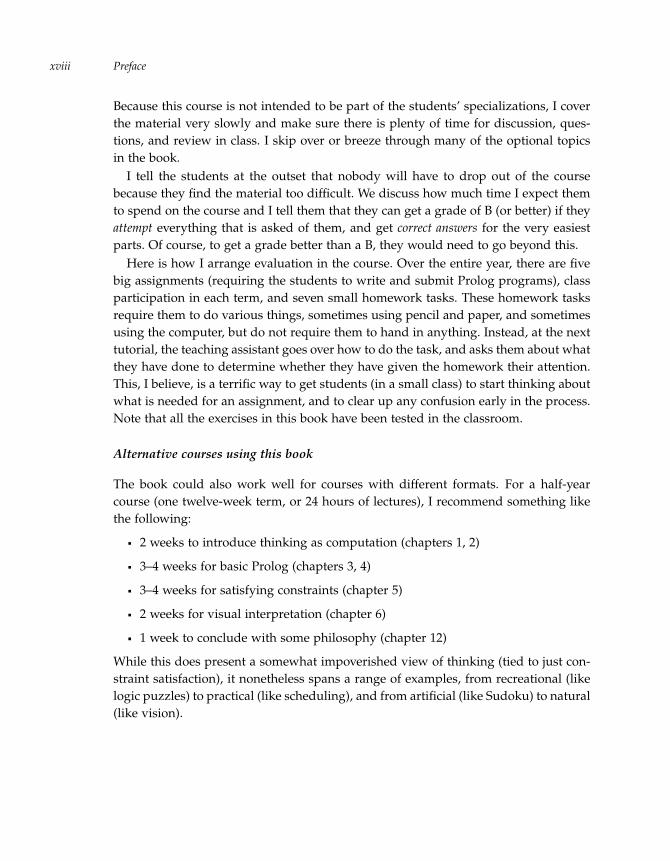
The book could also work well for courses with different formats. For a half-yearcourse (one twelve-week term, or 24 hours of lectures), I recommend something likethe following:

2 weeks to introduce thinking as computation (chapters 1, 2)



2 weeks for visual interpretation (chapter 6)


While this does present a somewhat impoverished view of thinking (tied to just con-straint satisfaction), it nonetheless spans a range of examples, from recreational (likelogic puzzles) to practical (like scheduling), and from artificial (like Sudoku) to natural(like vision).

“run” — 2011/9/8 — 18:05 — page xix — #20�

�

�

�

�

�

�

�

Preface xix

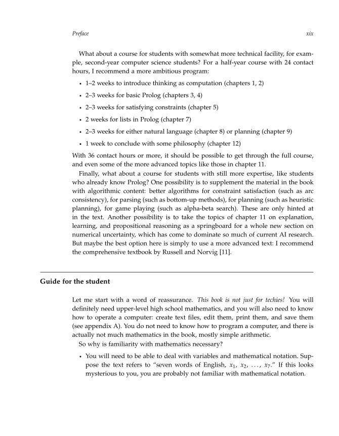
What about a course for students with somewhat more technical facility, for exam-ple, second-year computer science students? For a half-year course with 24 contacthours, I recommend a more ambitious program:

1–2 weeks to introduce thinking as computation (chapters 1, 2)



2 weeks for lists in Prolog (chapter 7)

2–3 weeks for either natural language (chapter 8) or planning (chapter 9)


With 36 contact hours or more, it should be possible to get through the full course,and even some of the more advanced topics like those in chapter 11.

Finally, what about a course for students with still more expertise, like studentswho already know Prolog? One possibility is to supplement the material in the bookwith algorithmic content: better algorithms for constraint satisfaction (such as arcconsistency), for parsing (such as bottom-up methods), for planning (such as heuristicplanning), for game playing (such as alpha-beta search). These are only hinted atin the text. Another possibility is to take the topics of chapter 11 on explanation,learning, and propositional reasoning as a springboard for a whole new section onnumerical uncertainty, which has come to dominate so much of current AI research.But maybe the best option here is simply to use a more advanced text: I recommendthe comprehensive textbook by Russell and Norvig [11].

Guide for the student

Let me start with a word of reassurance. This book is not just for techies! You willdefinitely need upper-level high school mathematics, and you will also need to knowhow to operate a computer: create text files, edit them, print them, and save them(see appendix A). You do not need to know how to program a computer, and there isactually not much mathematics in the book, mostly simple arithmetic.

So why is familiarity with mathematics necessary?

You will need to be able to deal with variables and mathematical notation. Sup-pose the text refers to “seven words of English, x1, x2, . . . , x7.” If this looksmysterious to you, you are probably not familiar with mathematical notation.

“run” — 2011/9/8 — 18:05 — page xx — #21�

�

�

�

�

�

�

�

Prefacexx

You will need to be able to look at large symbolic expressions (or formulas),make sure they are put together correctly, and work on them precisely accordingto instructions. You need to be able to deal with a lot of tiny details withoutgetting lost or bored. You might have picked up this skill in a variety of ways(like knitting from a complex pattern or building a model ship inside a bottle),but courses in mathematics are terrific practice.

Assuming you are interested in the subject matter of the book, do you have thenecessary background to get through it all? There is no easy answer. I suggest youwork through the first few chapters until you get to the exercises in chapter 4. If youhave no idea of how to do the first few exercises there, then you should certainlyconsider stopping.

Going through this book as a self-study course is much harder than having aninstructor who can answer questions as they come up. But if you are going throughit alone, here are some things you definitely need to know:

Any chapter or section with an asterisk (∗) marking the title is an optional topicthat may be more advanced. (A marked section within a marked chapter is evenmore advanced.) Skip these on first reading, or at least don’t be disappointed ifthey are not clear to you at first.

The exercises at the end of each chapter range from very simple to much moredifficult. You should always be able to answer the first few questions, but don’tbe discouraged if you can’t get through all of them.

“run” — 2011/9/8 — 18:05 — page xxi — #22�

�

�

�

�

�

�

�

Acknowledgments

This book has its genesis in a course that the late Ray Reiter and I first taught togetherin 1994. It was Ray who had the idea of teaching logic programming, including theconcept of recursion, to first-year undergraduates. I owe Ray an enormous debt forhis inspiration and intellectual leadership on this, and I can only hope that he wouldhave found this book to his liking.

Over the years, the course evolved and began to be less about programming andmore about artificial intelligence. I thank all the students who went through vari-ous iterations of the course without a textbook, as well as the teaching assistants:David Mitchell, Mikhail Soutchanski, Ron Petrick, Stavros Vassos, and Tim Capes.I also thank the University of Toronto for giving me the opportunity to teach anexperimental and ever-changing course to first-year students.

I was fortunate that a number of people were willing to read drafts of parts of thebook and provide me with comments: Ron Brachman, Ernie Davis, Sven Dickinson,Gerhard Lakemeyer, Gerald Penn, Bart Selman, Mikhail Soutchanski, my brothersJohn and Paul, my daughter Michelle, and three anonymous reviewers. Their com-ments were invaluable! I thank them all. All the remaining errors and oversights inthe book are of course my fault, not theirs.

I also wish to thank the good folks at MIT Press. Ada Brunstein and Marc Lowen-thal believed in the project from the very beginning and helped to get me started.Mel Goldsipe saw me through the many final edits and helped to get me stopped. Aspecial thanks to Alice Cheyer for her thorough copyediting.

This book was completed while I was on sabbatical from the University of Toronto.I thank my hosts Gerhard Lakemeyer at the Technical University of Aachen, MauricePagnucco at the University of New South Wales, and Jim Delgrande at Simon FraserUniversity for providing such wonderful environments for writing. I also thank theNatural Science and Engineering Research Council of Canada who generously fundedme throughout the writing of the book, and in fact, throughout my academic career.

Finally, I would like to thank my family and friends who supported me most enthu-siastically throughout the project, and especially Pat, my dearest wife and proofreaderextraordinaire, who might have heard “Working on the book!” a bit too often as theanswer to the question “What are you doing today?” Well guys, it’s all done!

Toronto, August 2011

“run” — 2011/9/8 — 18:05 — page xxii — #23�

�

�

�

�

�

�

�

“run” — 2011/9/8 — 18:05 — page 1 — #24�

�

�

�

�

�

�

�

1 Thinking and Computation

Consider the following scenario:

A professor enters a classroom where a group of undergraduates is sitting, andannounces “There is free pizza in the hall!” Suddenly, the students stand up andstampede toward the classroom door.

The events described here seem so ordinary that it is easy to miss how truly remark-able they are. But step back from them for a moment and imagine that you arestudying these students as a curious scientist from another world. You observe that acertain sound emanates from the professor and that this causes a flurry of activity inthe students. Now, as a scientist, ask yourself this: What sort of physics would explainhow acoustic energy can be transformed into kinetic energy in this way? In particu-lar, note that a very small change in the acoustic energy (like the professor’s saying“There is free pizza in Nepal.”) can result in no kinetic energy being produced at all,except maybe for some puzzled head shaking.

This is the wonder of intelligent behavior, perhaps the single most complex naturalphenomenon that we are aware of. As a sheer mystery, it easily overshadows topicslike dark matter, the source of gravity, and the mechanics of cancer.

One striking aspect of intelligent behavior of this sort is that it is clearly conditionedby knowledge: for a very wide range of activities, people make decisions about whatto do based on what they know (or believe) about the world, effortlessly and oftenunconsciously. It’s certainly not the sounds themselves that cause the students to standup like animals that have been trained to respond to a bell. This is easy enoughto confirm. The professor could have brought in a sign with a pizza message on itwritten in big letters, and the effect would have been just the same. In fact, one canimagine a situation where the following is written on the whiteboard at the front ofthe classroom:

As part of a psychology experiment, the professor will soon enter and tell youthat free food is available. This is just a test. Please remain seated.

In this case, neither the sounds nor the sign would have any effect at all. One cantry other small variations, and it will become clear that what makes the difference iswhether the students come to believe there is free pizza to be had nearby.

“run” — 2011/9/8 — 18:05 — page 2 — #25�

�

�

�

�

�

�

�

Chapter 12

Using what we believe or know in this way is so commonplace that we only reallypay attention to it when it is not there. When we say that someone behaved unintel-ligently, for instance, when someone uses a lit match to see if there is any gas in acar’s gas tank, what we usually mean is not that there is something the person didnot know but rather that the person has failed to use what he or she did know. Wemight say: “You weren’t thinking!” Indeed, it is thinking that is supposed to deliverwhat we know to the decisions we need to make. The students head toward the doorbecause they think that is the way to free pizza. It is thinking, in the end, that makeshuman behavior intelligent.

But what is thinking, and how does it work? What exactly goes on in people’sheads when they think about where to go for free pizza, or about who will win theAcademy Award for Best Actor, or about whether a free market needs to be regulated?

The purpose of this book is to suggest where to look for an answer. It proposes thatthinking is a form of computation. In the same way that digital computers performcalculations on representations of numbers, human brains perform calculations onrepresentations of what is known.

This chapter is an introduction to this idea. The first section reviews very brieflythe notion of thinking. The process of computation is somewhat less familiar, so moretime is spent on it, in the second section. The third section introduces the (somewhatcontroversial) idea of thinking as a form of computation.

1.1 Thinking

Are brains like computers? In a word, no. It is true historically that in trying tounderstand the brain, people have proposed models that seem to mirror the mostadvanced technology of the time. Over the years, the brain has been described asclockwork, a steam engine, a telephone switchboard, and (these days) a computer.But in time, these descriptions are found to be much too simplistic to say anythinguseful about what is inside our heads. There is no reason to believe that the computeranalogy will be any different in this regard.

In fact, this book has very little to say about the brain itself. Rather it focuses onthinking. But thinking is what the brain does. How can one study the relation betweencomputers and thinking without studying the brain?

Here is a useful analogy. Consider the study of flight (in the days before airplanes).One might want to understand how certain animals like birds and bats are able to fly.

“run” — 2011/9/8 — 18:05 — page 3 — #26�

�

�

�

�

�

�

�

Thinking and Computation 3

One might also want to try to build machines that are capable of flight. There are twoways to proceed:

study flying animals like birds, looking very carefully at their wings, theirfeathers, their muscles, and then construct machines that emulate birds;

study aerodynamics—how air flows above and below an airfoil, and how thisprovides lift—by using wind tunnels and varying the shapes of airfoils.

Both kinds of studies lead to insights, but of a different sort. The second strategy is themore general one: it seeks to discover the principles of flight that apply to anything,including birds.

It is this second strategy that is used here to study thinking. While there is a lotto be learned by studying the brain, this book focuses on the thinking process itself todetermine general principles that will apply to brains and to anything else that needsto think.

1.1.1 What is thinking?

What exactly is thinking? For humans, it is clearly some sort of process that occurs inour heads over time. The easiest way to understand it is to observe it in action.

Read the following sentence:

The trophy would not fit into the brown suitcase because it was too small.

Pause for a moment to make sure you understand it. Now answer this question: Whatwas too small? What does it refer to? Clearly, it refers to the suitcase, not the trophy.

Now, how did you get the right answer?Observe that there is nothing in the sentence itself that gives away the answer. This

is easy to demonstrate. Simply replace the word small by big:

The trophy would not fit into the brown suitcase because it was too big.

What was too big? Now the answer goes the other way: it now refers to the trophy,not the suitcase.

What this shows is that in making sense of the sentence, in particular, in determin-ing what it refers to, you had to use what you already knew about the sizes of things,things fitting inside other things, and so on, even if you were unaware of doing so.

This is thinking.Thinking is bringing what you know to bear on what you are doing. This is what

you had to do to understand the sentence. The process happens in the brain, some-times very quickly, and you may or may not be aware that it is taking place. (You may

“run” — 2011/9/8 — 18:05 — page 4 — #27�

�

�

�

�

�

�

�

Chapter 14

not have felt the change that happened in your thinking when the word was changedfrom small to big.)

Thinking is clearly a biological process, since we are biological creatures. Does thismean that thinking is like digestion? Or like mitosis in cells? Or is it different still?

The central conjecture of this book is this:

Thinking can be usefully understood as a computational process.

Thinking has perhaps more in common with multiplication or sorting a list ofnumbers than with digestion or mitosis.

This conjecture is controversial. Not all philosophers, psychologists, evolutionarybiologists, and neuroscientists are lined up to support it. Some do, some don’t, andsome struggle with the concept of thinking in the first place.

Nonetheless this is the conjecture that this book pursues.

1.2 Computation

Computer science as a field of study has two branches: hardware and software.Hardware is the concern of engineers who study and build the physical machines(computers) themselves. Software is the written instructions—programs—specifyingwhat those machines should do. And what the machines do is computation, a certainmanipulation of symbols. Birds “produce” flight, musicians “produce” music, andcomputers “produce” computation according to a program.

This book focuses on computation itself as the primary subject of computer sci-ence. What (or who) is performing the symbol manipulation is a secondary concern.Modern electronic computers happen to provide a fast, cheap, and reliable way to dothis computation, but other devices can do it as well. (The Dutch computer scientistEdsger Dijkstra once said that computer science is no more about the computers thanastronomy is about telescopes.)

1.2.1 Symbols and symbolic structures

In their simplest form, symbols are just characters from some alphabet, like thefollowing:

digits: 3, 7, V (the last one is a Roman numeral)

letters: x, R, β (the last one is a Greek letter)

operators: +, ≤ , ∩

“run” — 2011/9/8 — 18:05 — page 5 — #28�

�

�

�

�

�

�

�


They can be strung together into more complex forms:

numerals: 5874, –3.75

words: John, don’t

They can be grouped in certain ways:

mathematical expressions: 247 + 4(x – 1)3

English phrases: the woman John loved

Finally, some of these groupings can be thought of as being true or false:

mathematical inequalities: 247 + 4(x – 1)3 ≤ n!

4

English sentences: The woman John loved had brown hair.

It is symbolic structures, arrangements of symbols like those just illustrated, that arethe medium of computation.

1.2.2 What is computation?

For present purposes, computation is the process of taking symbolic structures, break-ing them apart, comparing them, and reassembling them according to a precise recipecalled a procedure. The symbols at the start of the procedure are called the inputs. Thesymbols at the end of the procedure are called the outputs. The procedure is called onthe inputs and returns the outputs. It is important to keep track of where you are andto follow the instructions in the procedure exactly. (You may not be able to figure outwhy you are doing the steps involved. No matter.)

1.2.3 Some arithmetic procedures

Imagine explaining to someone (a young child) how to do subtraction:

53– 17

One might say something like this:

First subtract the 7 from 3. But since since 7 is bigger than 3, borrow 10 from the5 on the left. That changes the 3 to a 13 and changes the 5 to a 4. So subtract 7not from 3 but from 13, which gives 6. Write the 6 as the first digit of the answeron the right, under the 7. Then subtract 1 not from 5 but from 4, which gives 3.Write the 3 as the second digit of the answer, under the 1. So the answer is 36.

“run” — 2011/9/8 — 18:05 — page 6 — #29�

�

�

�

�

�

�

�

Chapter 16

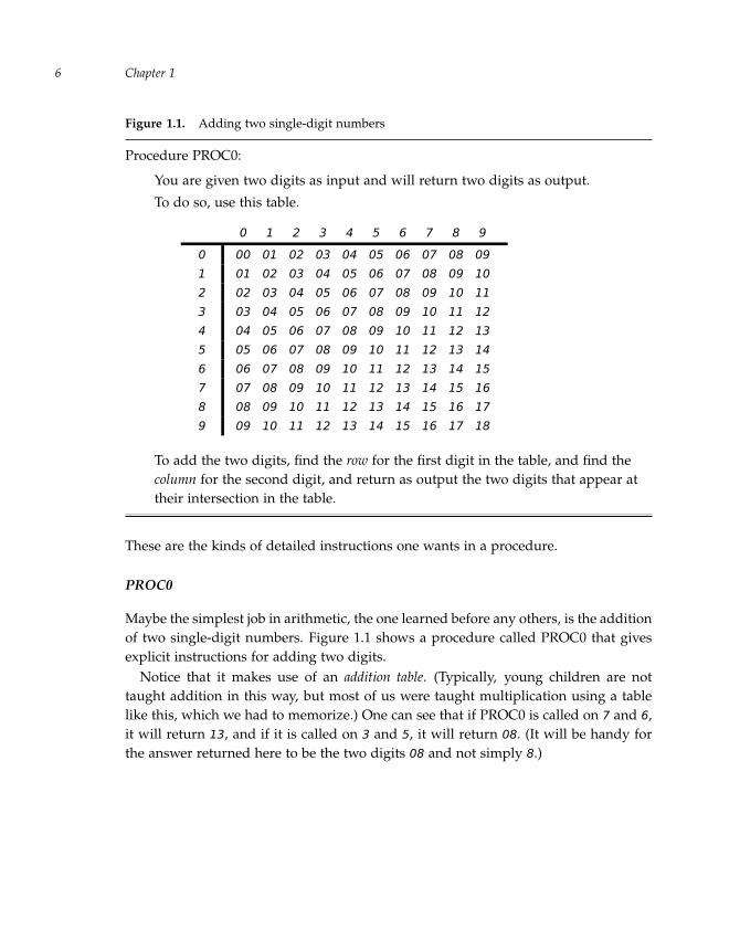
Figure 1.1. Adding two single-digit numbers

Procedure PROC0:

You are given two digits as input and will return two digits as output.

To do so, use this table.

0 1 2 3 4 5 6 7 8 9

0 00 01 02 03 04 05 06 07 08 09

1 01 02 03 04 05 06 07 08 09 10

2 02 03 04 05 06 07 08 09 10 11

3 03 04 05 06 07 08 09 10 11 12

4 04 05 06 07 08 09 10 11 12 13

5 05 06 07 08 09 10 11 12 13 14

6 06 07 08 09 10 11 12 13 14 15

7 07 08 09 10 11 12 13 14 15 16

8 08 09 10 11 12 13 14 15 16 17

9 09 10 11 12 13 14 15 16 17 18

To add the two digits, find the row for the first digit in the table, and find thecolumn for the second digit, and return as output the two digits that appear attheir intersection in the table.

These are the kinds of detailed instructions one wants in a procedure.

PROC0

Maybe the simplest job in arithmetic, the one learned before any others, is the additionof two single-digit numbers. Figure 1.1 shows a procedure called PROC0 that givesexplicit instructions for adding two digits.

Notice that it makes use of an addition table. (Typically, young children are nottaught addition in this way, but most of us were taught multiplication using a tablelike this, which we had to memorize.) One can see that if PROC0 is called on 7 and 6,it will return 13, and if it is called on 3 and 5, it will return 08. (It will be handy forthe answer returned here to be the two digits 08 and not simply 8.)

“run” — 2011/9/8 — 18:05 — page 7 — #30�

�

�

�

�

�

�

�


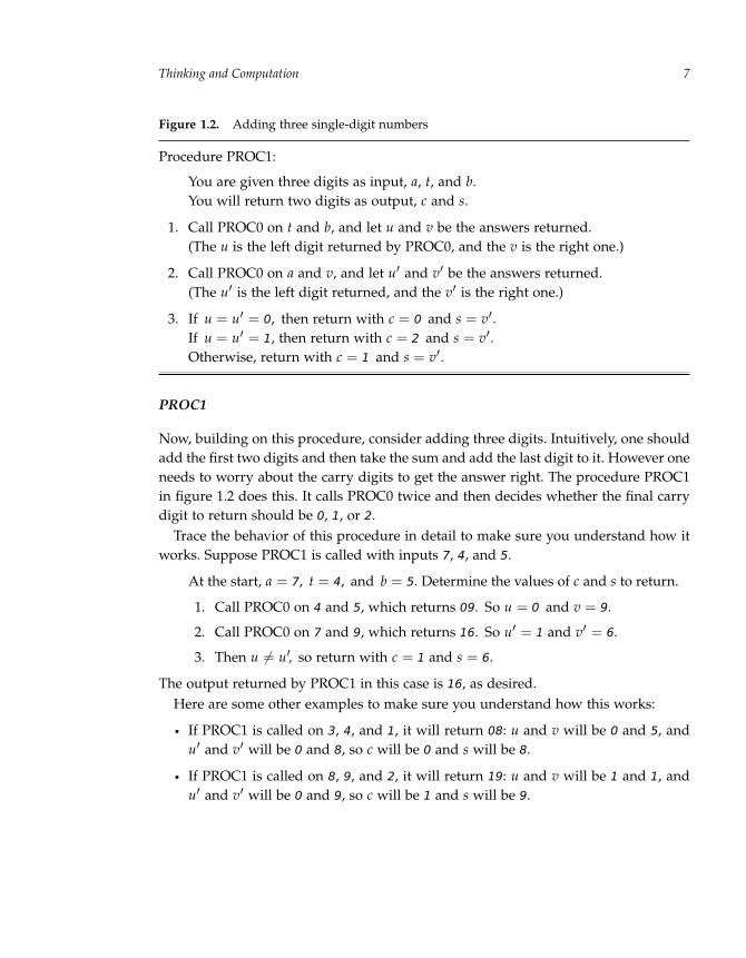
Figure 1.2. Adding three single-digit numbers

Procedure PROC1:

You are given three digits as input, a, t, and b.You will return two digits as output, c and s.

1. Call PROC0 on t and b, and let u and v be the answers returned.(The u is the left digit returned by PROC0, and the v is the right one.)

2. Call PROC0 on a and v, and let u′ and v′ be the answers returned.(The u′ is the left digit returned, and the v′ is the right one.)

3. If u = u′ = 0, then return with c = 0 and s = v′.If u = u′ = 1, then return with c = 2 and s = v′.Otherwise, return with c = 1 and s = v′.

PROC1

Now, building on this procedure, consider adding three digits. Intuitively, one shouldadd the first two digits and then take the sum and add the last digit to it. However oneneeds to worry about the carry digits to get the answer right. The procedure PROC1in figure 1.2 does this. It calls PROC0 twice and then decides whether the final carrydigit to return should be 0, 1, or 2.

Trace the behavior of this procedure in detail to make sure you understand how itworks. Suppose PROC1 is called with inputs 7, 4, and 5.

At the start, a = 7, t = 4, and b = 5. Determine the values of c and s to return.

1. Call PROC0 on 4 and 5, which returns 09. So u = 0 and v = 9.

2. Call PROC0 on 7 and 9, which returns 16. So u′ = 1 and v′ = 6.

3. Then u �= u′, so return with c = 1 and s = 6.

The output returned by PROC1 in this case is 16, as desired.Here are some other examples to make sure you understand how this works:

If PROC1 is called on 3, 4, and 1, it will return 08: u and v will be 0 and 5, andu′ and v′ will be 0 and 8, so c will be 0 and s will be 8.


“run” — 2011/9/8 — 18:05 — page 8 — #31�

�

�

�

�

�

�

�

Chapter 18

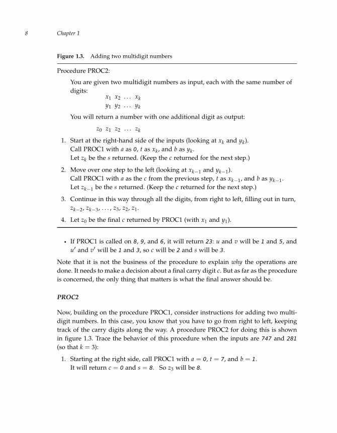
Figure 1.3. Adding two multidigit numbers

Procedure PROC2:

You are given two multidigit numbers as input, each with the same number ofdigits:

x1 x2 . . . xky1 y2 . . . yk

You will return a number with one additional digit as output:

z0 z1 z2 . . . zk

1. Start at the right-hand side of the inputs (looking at xk and yk).Call PROC1 with a as 0, t as xk, and b as yk.Let zk be the s returned. (Keep the c returned for the next step.)

2. Move over one step to the left (looking at xk−1 and yk−1).Call PROC1 with a as the c from the previous step, t as xk−1, and b as yk−1.Let zk−1 be the s returned. (Keep the c returned for the next step.)

3. Continue in this way through all the digits, from right to left, filling out in turn,zk−2, zk−3, . . . , z3, z2, z1.

4. Let z0 be the final c returned by PROC1 (with x1 and y1).


Note that it is not the business of the procedure to explain why the operations aredone. It needs to make a decision about a final carry digit c. But as far as the procedureis concerned, the only thing that matters is what the final answer should be.

PROC2

Now, building on the procedure PROC1, consider instructions for adding two multi-digit numbers. In this case, you know that you have to go from right to left, keepingtrack of the carry digits along the way. A procedure PROC2 for doing this is shownin figure 1.3. Trace the behavior of this procedure when the inputs are 747 and 281

(so that k = 3):

1. Starting at the right side, call PROC1 with a = 0, t = 7, and b = 1.It will return c = 0 and s = 8. So z3 will be 8.

“run” — 2011/9/8 — 18:05 — page 9 — #32�

�

�

�

�

�

�

�


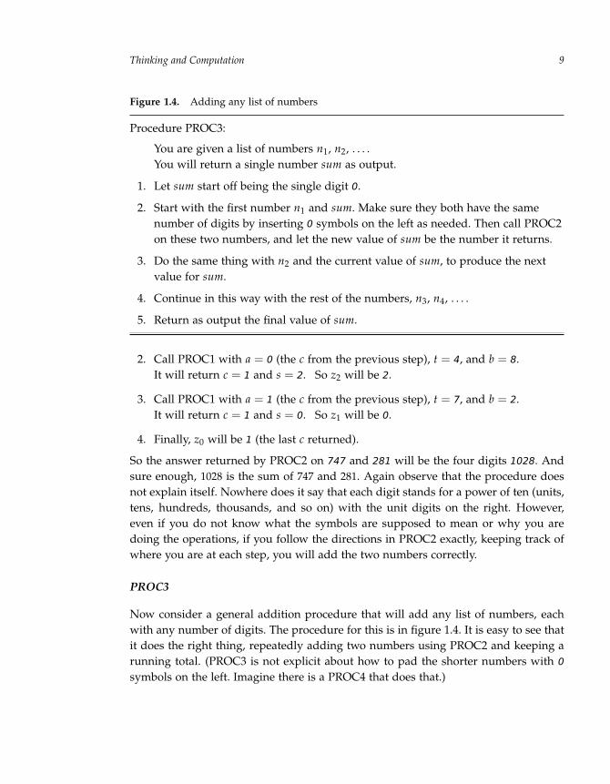
Figure 1.4. Adding any list of numbers

Procedure PROC3:

You are given a list of numbers n1, n2, . . . .You will return a single number sum as output.

1. Let sum start off being the single digit 0.

2. Start with the first number n1 and sum. Make sure they both have the samenumber of digits by inserting 0 symbols on the left as needed. Then call PROC2on these two numbers, and let the new value of sum be the number it returns.

3. Do the same thing with n2 and the current value of sum, to produce the nextvalue for sum.

4. Continue in this way with the rest of the numbers, n3, n4, . . . .

5. Return as output the final value of sum.

2. Call PROC1 with a = 0 (the c from the previous step), t = 4, and b = 8.It will return c = 1 and s = 2. So z2 will be 2.

3. Call PROC1 with a = 1 (the c from the previous step), t = 7, and b = 2.It will return c = 1 and s = 0. So z1 will be 0.

4. Finally, z0 will be 1 (the last c returned).

So the answer returned by PROC2 on 747 and 281 will be the four digits 1028. Andsure enough, 1028 is the sum of 747 and 281. Again observe that the procedure doesnot explain itself. Nowhere does it say that each digit stands for a power of ten (units,tens, hundreds, thousands, and so on) with the unit digits on the right. However,even if you do not know what the symbols are supposed to mean or why you aredoing the operations, if you follow the directions in PROC2 exactly, keeping track ofwhere you are at each step, you will add the two numbers correctly.

PROC3

Now consider a general addition procedure that will add any list of numbers, eachwith any number of digits. The procedure for this is in figure 1.4. It is easy to see thatit does the right thing, repeatedly adding two numbers using PROC2 and keeping arunning total. (PROC3 is not explicit about how to pad the shorter numbers with 0

symbols on the left. Imagine there is a PROC4 that does that.)

“run” — 2011/9/8 — 18:05 — page 10 — #33�

�

�

�

�

�

�

�

Chapter 110

Going from here

Given a procedure that can do addition, it is not too hard to imagine doing subtractionthe same way. Given those two, one can define procedures that do multiplication anddivision. Building on these, one can have a procedure to tell whether a number isprime. One can use pairs of numbers to represent fractions (rational numbers) anddo arithmetic on them. One can arrange rational numbers into matrices and haveprocedures that operate on them to solve systems of equations. One can use systemsof equations to model complex physical systems and have procedures that performnumerical simulations of these systems.

And on it goes.So starting with simple symbolic operations (such as table lookup, putting together

and taking apart sequences of symbols, comparing them, and so on), one can assem-ble the operations into ever larger procedures and develop an extremely wide rangeof behaviors as computational processes. This is what computer science is about.

1.2.4 The lesson

The key observation on these arithmetic procedures is this:

To produce meaningful answers, you do not have to understand what the symbolsstand for or why the manipulations are correct.

Although one can certainly understand the procedures as doing arithmetic, one doesnot need this understanding to actually carry out the procedures.

Here is a simple thought experiment to support this claim. Imagine replacing thesymbols 0 through 9 everywhere by new symbols that do not look at all like digits, forexample, a heart shape for 0, a star for 1, an anchor shape for 2, and so on. Now givethe procedures PROC0–PROC3, including the table for PROC0 with the new symbols,to a friend without saying what these new symbols mean or what the procedures aresupposed to be doing. By following PROC2, the friend should still be able to doaddition: take as input two sequences of new symbols representing numbers, andreturn as output the sequence of new symbols that represents their sum.

So symbols can be processed purely mechanically and still end up producing theright results. This might be called the trick of computation:

Computers can perform a wide variety of impressive activities precisely becausethose activities can be described as a type of symbol processing that can be carriedout purely mechanically.

“run” — 2011/9/8 — 18:05 — page 11 — #34�

�

�

�

�

�

�

�


This “trick” has turned out to be one of the major inventions of the twentieth cen-tury, allowing devices that perform computation to permeate almost all areas of ourmodern lives. And note: It has nothing to do with electronics or physics.

1.3 Thinking as computation

One might still ask, though, just what does computation have to do with ordinarythinking? Recall the central conjecture of this book:

Thinking can be usefully understood as a computational process.

What does this conjecture amount to?

Not that the brain is something like an electronic computer (which it is in someways perhaps, but in most ways is not).

The process of thinking can be usefully understood as a form of symbol processingthat can be carried out purely mechanically without having to know what thesymbols stand for.

Why is this so controversial? Perhaps the idea that some types of thinking are com-putational is not so surprising. Consider activities like doing a homework problemin algebra, or filling out an income tax form, or estimating a grocery bill as you areshopping. These all involve thinking and are clearly computational.

The problem is that so much of our thinking seems to have very little to do withcalculations or anything even remotely numerical. You can think about anything youwant, not just numbers. Consider this example:

I know my keys are in my coat pocket or on the fridge.That’s where I always leave them.

I felt in my coat pocket, and there’s nothing there.

So my keys must be on the fridge, and that’s where I should look.

This is an example of thinking that appears to have nothing to do with numbers. Butit is about something: keys, coat pocket, refrigerator. In fact, thinking always seems tobe about something. Computation, on the other hand, seems to be about nothing: it isthe process of manipulating symbols in a mechanical way without taking into accountwhat the symbols stand for. So there is certainly a conceptual gap between the twothat needs to be bridged. Fortunately, the bulk of the groundwork was already doneby Leibniz.

“run” — 2011/9/8 — 18:05 — page 12 — #35�

�

�

�

�

�

�

�

Chapter 112

1.3.1 Leibniz and his idea

The idea that thinking can be seen as a kind of computation is one of the rare ideas inWestern culture that does not go back to the ancient Greeks. The first person to takethis idea seriously was the German philosopher Gottfried Leibniz (1646–1716).

Leibniz was an amazing thinker. Among many other ideas and discoveries, heinvented the calculus at the same time as Isaac Newton did. While Newton was inter-ested in problems in physics and chemistry, Leibniz was more interested in symbolsand symbol manipulation. He only started doing mathematics seriously later in life.But intrigued by how symbols standing for variables and constants could be shuf-fled around to solve equations in algebra, he wondered whether there were symbolicsolutions to problems involving tangents and areas. And the infinitesimal calculus(derivatives and integrals) came out of this.

When it came to arithmetic, Leibniz observed that it was sufficient to manipulatesymbols on a piece of paper according to certain rules to be able to draw conclusionsabout otherwise abstract numbers. A number (like fourteen, say) might be a com-pletely abstract notion, but the symbols used to represent it (like the symbols 14 orXIV or 1110) are much more tangible: we can write them down, look at them, movethem around. We can determine if a certain relation holds among these numbers (forexample, determining whether a number is the sum of two others) just by manipu-lating the symbols. (The symbols 1110 represent the number fourteen in the binarynumber system invented by Leibniz that is used by digital computers.)

His idea then was this: Ideas, that is, the objects of ordinary thought, are like num-bers. It will be sufficient to manipulate symbols standing for them according to certainrules. The ideas may be abstract, but the symbols are concrete. One will be able to gofrom one idea to the next just by doing symbolic manipulation.

In other words, he drew the following analogy:

The rules of arithmetic allow us to deal with abstract numbers in terms of con-crete symbols. The manipulation of those symbols mirrors the relations amongthe numbers being represented.

The rules of logic allow us to deal with abstract ideas in terms of concrete sym-bols. The manipulation of those symbols mirrors the relations among the ideasbeing represented.

What a truly remarkable idea! It says that although the objects of human thought areformless and abstract, we can still deal with them concretely as a kind of arithmetic,by representing them symbolically and operating on the symbols.

“run” — 2011/9/8 — 18:05 — page 13 — #36�

�

�

�

�

�

�

�


In the case of arithmetic, we already know what numbers are and what symbols weshould use to represent them. We have all been trained to do this symbolic processingstarting at a very early age, without a second thought.

But what about ideas? What symbols should stand for them?

1.3.2 Propositions vs. sentences

A proposition, as the word is used in the philosophical literature, is an idea that canbe expressed by a declarative sentence of English (or other language). So one canthink of the sentence as a symbolic representation of the proposition. Consider theseexamples:

My keys are in my coat pocket.

Dinosaurs were warm-blooded.

The stock market composite index will rise to twice its current value within

the next three years.

Hate literature should not be tolerated, even if that impinges on free speech.

These are all English sentences. The first one uses seven words of English, for exam-ple. But apart from being English sentences, they each express an idea, an idea thatcan be expressed in other languages with other sentences. So we have the sentence, onthe one hand (like the first one with seven words), and the proposition it expresses, onthe other (like the idea that my keys are located somewhere).

What can be said about the propositions themselves? They are abstract entities, likenumbers, but they have some special properties:

Propositions are considered to hold or to not hold. A sentence is true if theproposition it expresses holds, and false if that proposition does not hold.

This does not mean that there will be no controversy about whether the propo-sition holds. It just means that it makes sense to ask if it holds (or if thecorresponding sentence is true). A number is a very different sort of abstractobject; we do not ask if a number holds in this sense.

Propositions are considered to be related to people in certain ways: people mayor may not believe them, fear them, regret them, wish for them, worry aboutthem, and so on. These various relationships between people and propositionsare what philosophers call propositional attitudes.

Propositions are related to each other in certain ways: a proposition might imply,or provide evidence for, or contradict another proposition.

“run” — 2011/9/8 — 18:05 — page 14 — #37�

�

�

�

�

�

�

�

Chapter 114

Uninterpreted sentences

A first clue that one might be able to understand thinking as computation is to look ata sentence of English as a purely symbolic structure made up of a sequence of words.Consider this, for example:

The snark was a boojum.

This is a line from the poem The Hunting of the Snark, by Lewis Carroll, that wasintended to be nonsense. (What is this snark? What is a boojum?) Observe that if oneassumes that the sentence is true, even without knowing what the words snark andboojum mean, one can answer certain questions:

What kind of thing was the snark?(It was a boojum.)

Is it true that the snark was either a beejum or a boojum?(Yes, because it was a boojum.)

If no boojum is ever a beejum, was the snark a beejum?(No, it could not have been.)

What is an example of something that was a boojum?(The snark, of course.)

The point is that one can provide appropriate answers to these questions withouthaving to know what the two symbols mean. This is the first step toward linking thinkingand computation. Some simple rules of logic make it possible to extract answersdirectly from the sentence itself (viewed as a symbolic structure) without having todetermine first what the symbols snark and boojum stand for.

Now consider the following three examples:

1. My keys are in my coat pocket or on the fridge.

Nothing is in my coat pocket.

So: My keys are on the fridge.

2. Henry is in the basement or in the garden.

Nobody is in the basement.

So: Henry is in the garden.

3. Jill is married to George or Jack.

Nobody is married to George.

So: Jill is married to Jack.

“run” — 2011/9/8 — 18:05 — page 15 — #38�

�

�

�

�

�

�

�


Observe that in all these cases the thinking is the same. The pieces are put togetherin exactly the same way, even though the sentences are about quite different things.There could just as easily be a fourth example:

4. The frumble is frimble or framble.

Nothing is frimble.

So: The frumble is framble.

Again, one does not need to know what frimble means to get the correct conclusion.It does not really matter whether the subject is keys, Henry, Jill, or the frumble. Whatdoes matter is the form of the sentences in terms of the other connecting words, andthe conclusion based on that form. For example, it would be wrong in the last case toconclude that the frumble was frimble.

Logical entailment

Telling us what to conclude in such examples is the job of logic. A collection ofsentences S1, S2, . . . , Sn logically entails another sentence S if the truth of S is implicitin the truth of the Si sentences. In other words, no matter what certain terms (likeboojum, garden, framble) in the Si sentences really mean, if they are all true, then theS sentence is also true. So, in determining if a collection of sentences logically entailsanother, it is not necessary to know what the terms in those sentences mean. (Certainkeywords in sentences, such as and, do have specific functions.)

So, for example, the sentence

The snark was a boojum.

logically entails

Something was a boojum.

Similarly, the sentences

My keys are in my coat pocket or on the fridge.

Nothing is in my coat pocket.

logically entail

My keys are on the fridge.

The fact that these symbols can be used in an uninterpreted way is what allows theconnection with computation.

“run” — 2011/9/8 — 18:05 — page 16 — #39�

�

�

�

�

�

�

�

Chapter 116

Is thinking logic?

So in the end, is thinking just logic? For anyone who has studied logic, this is not avery plausible notion.

Suppose somebody at a party says,

George is a bachelor.

Here are some of the sentences that this logically entails:

Somebody is a bachelor.

George is either a bachelor or a pig farmer.

Not everyone is not a bachelor.

It is not the case that both George and Henry are not bachelors.

Sure enough, these sentences will all be true if the given sentence is; that is whatlogical entailment does. But they are so very, very boring!

If you found out at a party that George was a bachelor, it is almost guaranteed thatwe would not spend time going through logical entailments like these. You mightthink about George (whom you might already know) or about what it means to bea bachelor. Thinking seems to be so much richer than just dry logical entailmentsbecause thinking seems to depend on what the words in a sentence mean.

In fact, the view that thinking is logic may seem so far off the mark that instead ofasking what is wrong with it, one might be tempted to ask what is right with it.

1.3.3 Using what is known: The web of belief

To get a glimmer of what could be right with it, one has to go back to the ideaof thinking: bringing knowledge to bear on an activity. In reaching the conclusionsabout George the bachelor, no other knowledge was used. The search for logicalentailments is not from that one sentence alone but rather from that sentence togetherwith everything else that is already known.

Figure 1.5 shows some of the relevant facts that may be known about George thebachelor. In this collection of sentences, the terms George, bachelor, man, and so on,appear in many places, linking the sentences together in the same way that the termfrimble did in the sentences of the earlier example.

It is sometimes helpful to visualize the sentences as forming a kind of network, withnodes for each of the terms and links between them according to the sentences inwhich they appear. The network might look something like the one in figure 1.6. Wemay not know who George is, for example, but we can see that the node for Georgeis connected to the node for Mary by way of the node for son. We may not know what

“run” — 2011/9/8 — 18:05 — page 17 — #40�

�

�

�

�

�

�

�


Figure 1.5. Some beliefs about George the bachelor

George was born in Boston, collects stamps.

George is the only son of Mary and Fred.

A son of someone is a child who is male.

A man is an adult male person.

A bachelor is a man who has never been married.

A (traditional) marriage is a contract between a man and a woman that is enacted by a

wedding and dissolved by a divorce. While the contract is in effect, the man (called the

husband) and the woman (called the wife) are said to be married.

A wedding is a ceremony where . . . bride . . . groom . . . bouquet . . .

and so on.

son is supposed to mean, but its node is connected to the nodes for child and male.Similarly, the male node is connected in a different way to the node for man. Thenode for bachelor is connected in a complex way to the node for marriage and fromthere, presumably, to wedding and bride. Although we may not know what any ofthese terms mean in isolation, the various sorts of links given by the sentences in thenetwork provide a rich set of interdependencies among them.

A network like this is sometimes called a web of belief to emphasize that the sen-tences do not stand alone but link to many others by virtue of the terms they use. Thejob of logical entailment is to crawl over this web looking for connections among thenodes, sensitive to the different types of links along the way. In figure 1.6 there is acertain path from George to male, for example, that can lead to the conclusion thatGeorge is male. If the fact that George is a bachelor is added to the web, a new set ofpathways opens, including some connections from George to marriage that were notthere before.

The logical entailments for the new sentence together with everything previouslyknown gives some additional answers:

George has never been the groom at a wedding.

Mary has an unmarried son born in Boston.

No woman is the wife of any of Fred’s children.

These are much more like the ordinary thoughts that people would think when learn-ing that George was a bachelor. They are not exactly poignant, of course, but if some

“run” — 2011/9/8 — 18:05 — page 18 — #41�

�

�

�

�

�

�

�

Chapter 118

Figure 1.6. Some beliefs as a network

� was � in � , . . . . . .

George born Boston Fred

� is the only � of � and �

son Mary child

A � of someone is a � who is �

adult male

A � is an � � �

man person

A � is a � who has never been �

bachelor marriage contract married

A � is a � . . . . . . said to be �

��

��

��

��

��

��

��

��

��

��

��

additional facts were added about how parents hope their children end up happilymarried, one could go in that direction. (Or one might want to include facts aboutwhat a bachelor lifestyle is like and get additional entailments about George thatwould fit into a party setting.)

Observe that to get this richer set of conclusions, one does not need to know inadvance what the symbols George and bachelor mean. What is needed, however, is amuch richer collection of sentences over which to apply the rules of logic.

Knowledge bases

At this point, we have to be prepared to make a gigantic leap of the imagination:

Imagine that we can draw conclusions from millions of such facts.

In other words, to make a plausible connection between thinking and computing,we have to imagine that we are considering the logical entailments of a potentially

“run” — 2011/9/8 — 18:05 — page 19 — #42�

�

�

�

�

�

�

�


enormous collection of sentences, an entire web of belief. Such a collection is called aknowledge base (KB). The collection shown in figure 1.5 is just a very small sample.

So yes, there is a connection between thinking and logic, but it is misleading tothink of it as Logic, the subject studied in philosophy. The way Logic is normallytaught, one starts with a small set of premises and concentrates on ensuring that theconclusions from them are always correct:

Socrates is a man.All men are mortal.

Therefore, Socrates is mortal.

Thinking is very different. It starts with an enormous collection of premises (maybemillions of them) about a very wide array of subjects. There will be facts in the knowl-edge base about George and marriage, but also about barber shops, ferris wheels,Academy Awards, hate literature, and so on. The question then is, what are thelogical entailments of all those sentences?

This leads to two hypotheses:

Much of the subjective feeling of richness experienced in thinking might beexplained as simple mechanical and logical operations, but applied to a veryrich collection of sentences.

To build computer systems with a number of desirable properties (versatile,flexible, extendible, easily maintained, and so on), one must

– represent much of what the system needs to know as symbolic sentences ofsome sort, called its knowledge base;

– perform processing over the knowledge base using the rules of logic toobtain new conclusions;

– have the system act based on the conclusions it can derive.

Systems built this way are called knowledge-based systems.

The big picture

In summary, thinking means bringing what one knows to bear on what one is doing.But how does this work? How do concrete, physical entities like people engage withsomething formless and abstract like knowledge? What is proposed in this chapter(via Leibniz) is that people engage with symbolic representations of that knowledge. Inother words, knowledge is represented symbolically as a collection of sentences in aknowledge base, and then entailments of those sentences are computed as needed.

“run” — 2011/9/8 — 18:05 — page 20 — #43�

�

�

�

�

�

�

�

Chapter 120

(Actually, there are good reasons to deviate somewhat from strict logical entailmentfor this. See chapter 3.)

So computation over a knowledge base is the direction pursued in this book, althoughit deals with only tiny knowledge bases. The next chapter studies a procedure thatperforms this computation for knowledge bases of a certain restricted form.

Want to read more?

This chapter introduced the connection between thinking and computation, an ideathat is the subject matter of the rest of this book.

The starting point for this connection is the work of the philosopher Gottfried Leib-niz. A good introduction to his thinking can be found in [59]. (His own work isscattered in the thousands of letters he wrote.) There is not much in terms of details,however, as Leibniz did not have the benefit of the modern notions of symbolic logicor computation. These came along in the 1930s, and it took until the 1950s, when JohnMcCarthy, one of the founders of the field of artificial intelligence (AI) [11], becamethe first person to propose the approach followed in this book, representing what isknown as a collection of sentences and computing their logical entailments [47].

An excellent place to begin to explore what psychologists have to say about humanthinking is a book by Pinker [9] that is aimed at a broad audience. However, thewhole topic of human thinking remains highly controversial, and even Pinker has hisdetractors [3]. Many find the notion of symbolic computation too limiting becauseit downplays the effect of the rest of the body on the thinking process [2]. Amongthe computationalists, many prefer symbolic structures other than sentences that canrepresent knowledge in a more concrete way [5]. There are also researchers who feelthat a lot of thinking needs to be more pictorial or diagrammatic in nature [6].

The general notion of computation used here arose directly out of work on logicin the 1930s. This account of computation is due to Alan Turing, widely consideredto be the father of computer science (John von Neumann is often called the father ofelectronic computers). In 1936, Turing proposed a formal definition of what is herecalled a procedure in terms of a very simple imaginary device: a Turing machine [12].With this definition, one could now ask questions like whether it was even possible tocompute a certain result. Turing was the first to prove that there was a universal Turingmachine that could compute what any other one could, and remarkably enough, thatsome results could not be computed by any Turing machine.

“run” — 2011/9/8 — 18:05 — page 21 — #44�

�

�

�

�

�

�

�


Turing’s carefully worked definition has withstood the test of time. Although dif-ferent models of computation have been proposed (including a strikingly differentone by Alonzo Church), they have all been shown to be equivalent to Turing’s. Everycomputer built so far has been a special case of a Turing machine and subject to therestrictions proved by Turing. The claim that this will be true of any physical computerto be built is called the Church-Turing thesis [8].

Regarding thinking as computation, there is a superb though somewhat advancedphilosophical book on this subject by Pylyshyn [10]. Much of the argument presentedhere about how actions are conditioned by what is known derives from this insightfulbook. (In the terminology he uses, those actions are said to be cognitively penetrable.)

Outside of philosophy, there is a subarea of AI called knowledge representation andreasoning that starts with the work of McCarthy and is concerned with the issue ofrepresenting knowledge in symbolic form and devising computational procedures toreason with it effectively. A graduate-level textbook on this area of research is byBrachman and Levesque [1]. The state of the art in this research area is reviewed in a(quite advanced) technical handbook [4].

Finally, although this book concentrates on small knowledge bases, the CYC project[7] is an example of a project whose goal is to build a large knowledge base along thelines discussed here.

Exercise

Consider the procedure PROCX in figure 1.7. It assumes there are other procedureselsewhere that will do some arithmetic (subtraction, multiplication, and less-thancomparisons). It also assumes that one can concatenate strings of digits: x ˆy meansthe string consisting of the digits in x followed by those in y. It works by repeatedlysetting new values to u, v, bot, top, and side as the digits of the input are workedthrough in pairs from left to right.

Figure out what the procedure PROCX is doing. Hint: Trace its behavior when theinput is 137641.

“run” — 2011/9/8 — 18:05 — page 22 — #45�

�

�

�

�

�

�

�

Chapter 122

Figure 1.7. A mystery procedure

Procedure PROCX:

You are given a sequence of digits x as input.You will return a sequence of digits as output.

1. Group the digits in x into pairs starting from the right. (If x has an odd numberof digits, the leftmost group will only have a single digit in it.)

2. Start with u, v, bot, top, and side all having an initial value of 0.

3. Then, working your way from left to right on the groups in x,repeat the following:

a. Set bot to (bot − u) ˆ (the next group from x).

b. Set side to 2× top.

c. Set v to the largest single digit such that v × (side ˆv) ≤ bot.

d. Set u to v × (side ˆv).

e. Set top to top ˆv.

4. The answer to return is the final value of top.

“run” — 2011/9/8 — 18:05 — page 23 — #46�

�

�

�

�

�

�

�

2 A Procedure for Thinking

Chapter 1 showed that thinking, or at least some simple forms of thinking, couldbe profitably understood as drawing conclusions from a large collection of sentencescalled a knowledge base (KB). Leibniz’s idea was that the rules of logic would tell howto manipulate these symbolic structures representing propositions the same way thatthe rules of arithmetic tell how to manipulate symbolic structures representing num-bers. This chapter examines this symbolic manipulation as a computational procedure,not so different from those for arithmetic.

The procedure studied in this chapter is called back-chaining. It works on sentencesof English, but sentences that are very restricted in their form. They have none ofthe niceties found in English or any other natural language. On the other hand, thesesentences can be treated as uninterpreted symbolic structures: one can operate on themwithout having to know in advance what they mean. This is in accordance with theview of computation saying that one can produce interesting answers to interestingquestions without having to know what the symbols stand for.

This chapter has five sections. The first section looks at the types of sentencesincluded in the knowledge base and introduces a small example. Section 2 examinesthe notion of logical entailment in a bit more detail. The back-chaining procedure ispresented in section 3. Section 4 looks at some complex behavior of back-chaininginvolving variables. Section 5 summarizes very briefly what is good and less goodabout this procedure for thinking.

2.1 Atomic and conditional sentences

A special but very useful case of a knowledge base is one consisting of just two sortsof sentences:

Atomic sentences, that is, simple basic sentences whose exact form is leftunspecified for now

Conditional sentences, that is, sentences of the form If P1 and . . . and Pn then Q,where the Pi and the Q are atomic sentences

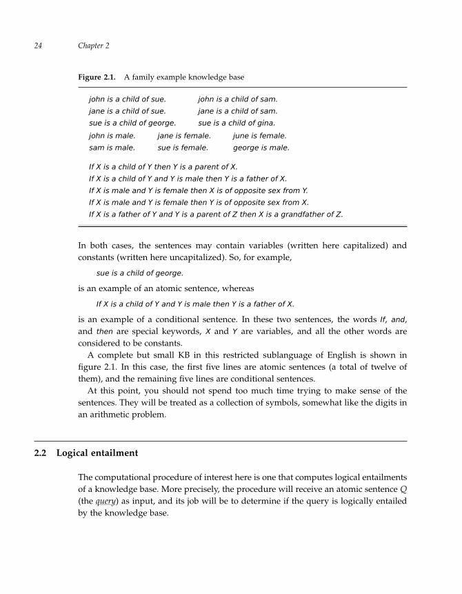
“run” — 2011/9/8 — 18:05 — page 24 — #47�

�

�

�

�

�

�

�

Chapter 224

Figure 2.1. A family example knowledge base

john is a child of sue. john is a child of sam.

jane is a child of sue. jane is a child of sam.

sue is a child of george. sue is a child of gina.

john is male. jane is female. june is female.

sam is male. sue is female. george is male.

If X is a child of Y then Y is a parent of X.

If X is a child of Y and Y is male then Y is a father of X.

If X is male and Y is female then X is of opposite sex from Y.

If X is male and Y is female then Y is of opposite sex from X.

If X is a father of Y and Y is a parent of Z then X is a grandfather of Z.

In both cases, the sentences may contain variables (written here capitalized) andconstants (written here uncapitalized). So, for example,

sue is a child of george.

is an example of an atomic sentence, whereas

If X is a child of Y and Y is male then Y is a father of X.

is an example of a conditional sentence. In these two sentences, the words If, and,and then are special keywords, X and Y are variables, and all the other words areconsidered to be constants.

A complete but small KB in this restricted sublanguage of English is shown infigure 2.1. In this case, the first five lines are atomic sentences (a total of twelve ofthem), and the remaining five lines are conditional sentences.

At this point, you should not spend too much time trying to make sense of thesentences. They will be treated as a collection of symbols, somewhat like the digits inan arithmetic problem.

2.2 Logical entailment

The computational procedure of interest here is one that computes logical entailmentsof a knowledge base. More precisely, the procedure will receive an atomic sentence Q(the query) as input, and its job will be to determine if the query is logically entailedby the knowledge base.

“run” — 2011/9/8 — 18:05 — page 25 — #48�

�

�

�

�

�

�

�

A Procedure for Thinking 25

Before going on to this procedure, it is worthwhile to examine the notion of logicalentailment more closely. Recall that a sentence is logically entailed if it cannot not helpbut be true if all the sentences in the knowledge base are true. In determining whatis and is not logically entailed, we do not use normal English understanding of theconstants that appear in the knowledge base or in the query. In the KB of figure 2.1,there are constants like sam and female; for purposes of logical entailment, imaginethat these names have been changed everywhere to something neutral, like object13

and property51.Here are some sample logical entailments of this knowledge base:

jane is a child of sue.

This sentence is in the KB, and therefore if everything in the KB is true, it mustbe true, too. Note that even if other symbols had been used everywhere in theKB and in the query, like relation17 instead of child and person53 instead of jane,the resulting sentence would still be an entailment.

sue is a parent of jane.

This sentence is not in the KB, but the following two sentences are there:

jane is a child of sue.


So if everything in the KB is true, then by virtue of the special keywords If andthen, the query must also be true. Again, this is not because of the relationshipbetween the English words child and parent; it is because there is a conditionalsentence in the KB that makes a connection between the child and parent symbols.

george is a grandfather of jane.

This sentence must be true for the same reason as the previous one; the argumentis just longer. It requires using these sentences in the KB:

1. george is male.

2. jane is a child of sue.

3. sue is a child of george.

4. If X is a child of Y then Y is a parent of X.

5. If X is a child of Y and Y is male then Y is a father of X.

6. If X is a father of Y and Y is a parent of Z then X is a grandfather of Z.

If everything in the KB is true, then the following sentences that are not in theKB must also be true:

“run” — 2011/9/8 — 18:05 — page 26 — #49�

�

�

�

�

�

�

�

Chapter 226

7. george is a father of sue. (by virtue of sentences 3, 1, and 5)

8. sue is a parent of jane. (by virtue of sentences 2 and 4)

9. george is a grandfather of jane. (by virtue of sentences 7, 8, and 6)

So in all three cases the query is logically entailed by the KB. Now let us considersome examples of sentences that are not logically entailed:

gina is female.

This sentence may indeed be true. After all, Gina is a name that is commonlyused by females. However, although the constant gina appears in the KB, it couldjust as well have been harvey or person17d. No connection to female is warranted.

john is younger than sam.

Someone might say, “If everything in the KB is true, then John is a child of Sam,so he has to be younger than Sam. So the query must be true.” This is not quiteright, but the reason may not be obvious. It cannot be assumed that the symbolyounger means the same as it does in English. In deciding what is entailed, theonly information that may be used is what actually appears in the KB (see parent

and grandfather). Since the symbol younger does not appear in the KB, there isno information to use. The query could be written as john is in relation239 to samwhich, of course, need not be true. So the query is not logically entailed.

sue is a mother of john.

This is similar to the previous case. The following two sentences are entailed bythe knowledge base:

sue is female.

sue is a parent of john.

But one cannot conclude that the sentence

sue is a mother of john.

is true. One might want to make a connection between mother and the symbolsfemale and parent, since that is how it works out in English. But nothing in theKB currently sanctions this. This is quite unlike the father case, where sentencesin the KB do connect father, male, and parent.

“run” — 2011/9/8 — 18:05 — page 27 — #50�

�

�

�

�

�

�

�


Figure 2.2. The back-chaining procedure

To establish a sentence Q:

1. Try to locate Q itself in the KB. If you can, then return success.

2. Otherwise, try to locate a conditional sentence of the form

If P1 and . . . and Pn then Q

in the KB. If you cannot, then return failure.

3. Otherwise, use back-chaining to try to establish P1, then P2, . . . , then Pn.If these are all successful, then return success.

4. Otherwise, go back to step 2 and look for another conditional.

2.3 Back-chaining

The computational procedure used in this chapter is called back-chaining. As men-tioned, the procedure is given an atomic sentence Q and attempts to determine if Qis logically entailed by the knowledge base, that is, back-chaining is asked to establishthe query. So the input will be a query Q (and implicitly, a KB in the background),and the output will be either success or failure. (Even if a query Q can be successfullyestablished, it is not added to the KB. Back-chaining always leaves the KB unchanged.No learning happens here.)

The back-chaining procedure is shown in figure 2.2. It is called back-chainingbecause it chains backward from a query to the atomic sentences in the KB. Notethat the back-chaining procedure for Q depends on using the back-chaining proce-dure for other sentences (the Pi). This makes it a recursive procedure (discussed inchapters 3 and 4). Before looking at back-chaining in action, we need to deal with onecomplication: variables.

2.3.1 Using variables

There are sentences in the knowledge base that include variables, such as the onerelating child and parent. A sentence like


is intended to work as if the KB included sentences like

“run” — 2011/9/8 — 18:05 — page 28 — #51�

�

�

�

�

�

�

�

Chapter 228

If john is a child of sue then sue is a parent of john.

If john is a child of gina then gina is a parent of john.

If gertrude is a child of heathcliff then heathcliff is a parent of gertrude.

and all the (infinitely many) other sentences of this form. So one needs to be able todraw the same conclusions from the one sentence with variables as would be drawnfrom all the other sentences with constants in them.

From the point of view of back-chaining, here is what this use of variables amountsto. Suppose the query Q is

george is a parent of sue.

Step 2 in figure 2.2 says to check whether the KB has a sentence of the form

If . . . then george is a parent of sue.

The KB does not have a conditional sentence for this particular Q, but it does have asentence

If . . . then Y is a parent of X.

This is considered to match the Q at step 2, so at step 3, the relevant Y is george andthe relevant X is sue. Here is the result:

The query Q at step 2 is george is a parent of sue.

The KB contains If X is a child of Y then Y is a parent of X.This is considered to match for Y=george and X=sue.

The query P1 at step 3 is sue is a child of george.

2.3.2 Tracing the back-chaining

The following four examples simulate the execution of the back-chaining procedureon four sample queries. This is called tracing the procedure and is very similar towhat was done with arithmetic in chapter 1. Note the step numbers as you follow theprocedure.

Example 1

Establish the query jane is a child of sue.

1. Look for jane is a child of sue in the KB. Found.Return success for jane is a child of sue.

“run” — 2011/9/8 — 18:05 — page 29 — #52�

�

�

�

�

�

�

�


Example 2

Establish the query gina is female.

1. Look for gina is female in the KB. Nothing found.

2. Look for If . . . then gina is female in the KB. Nothing found.Return failure for gina is female.

Example 3

Establish the query george is a father of sue.

1. Look for george is a father of sue in the KB. Nothing found.

2. Look for If . . . then george is a father of sue in the KB.Found: If X is a child of Y and Y is male then Y is a father of X.

This matches for Y=george and X=sue.

3. Work on the two if-parts of this matching conditional:(Note in figure 2.2 that the two parts are worked on from left to right.)

Establish the query sue is a child of george.(This is the query X is a child of Y with X=sue and Y=george.)

1. Look for sue is a child of george in the KB. Found.Return success for sue is a child of george.

Establish the query george is male.(This is the query Y is male with Y=george.)

1. Look for george is male in the KB. Found.Return success for george is male.

Since both parts were successful, return success for the original querygeorge is a father of sue.

Example 4

Establish the query jane is of opposite sex from george.

1. Look for jane is of opposite sex from george in the KB. Nothing found.

2. Look for If . . . then jane is of opposite sex from george in the KB.Found: If X is male and Y is female then X is of opposite sex from Y.

This matches for X=jane and Y=george.

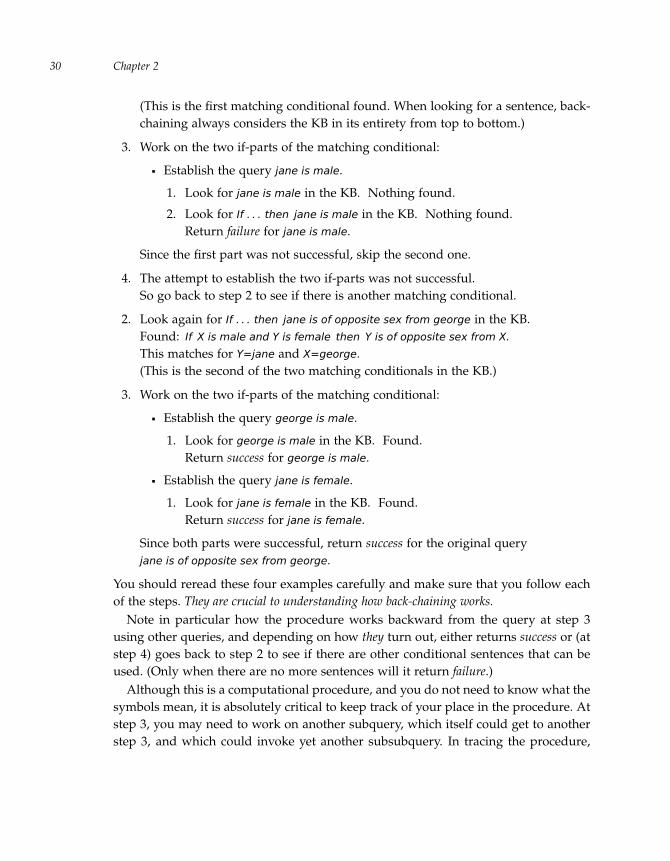
“run” — 2011/9/8 — 18:05 — page 30 — #53�

�

�

�

�

�

�

�

Chapter 230

(This is the first matching conditional found. When looking for a sentence, back-chaining always considers the KB in its entirety from top to bottom.)

3. Work on the two if-parts of the matching conditional:

Establish the query jane is male.

1. Look for jane is male in the KB. Nothing found.

2. Look for If . . . then jane is male in the KB. Nothing found.Return failure for jane is male.

Since the first part was not successful, skip the second one.

4. The attempt to establish the two if-parts was not successful.So go back to step 2 to see if there is another matching conditional.

2. Look again for If . . . then jane is of opposite sex from george in the KB.Found: If X is male and Y is female then Y is of opposite sex from X.

This matches for Y=jane and X=george.(This is the second of the two matching conditionals in the KB.)


Establish the query george is male.


Establish the query jane is female.

1. Look for jane is female in the KB. Found.Return success for jane is female.

Since both parts were successful, return success for the original queryjane is of opposite sex from george.

You should reread these four examples carefully and make sure that you follow eachof the steps. They are crucial to understanding how back-chaining works.

Note in particular how the procedure works backward from the query at step 3using other queries, and depending on how they turn out, either returns success or (atstep 4) goes back to step 2 to see if there are other conditional sentences that can beused. (Only when there are no more sentences will it return failure.)

Although this is a computational procedure, and you do not need to know what thesymbols mean, it is absolutely critical to keep track of your place in the procedure. Atstep 3, you may need to work on another subquery, which itself could get to anotherstep 3, and which could invoke yet another subsubquery. In tracing the procedure,

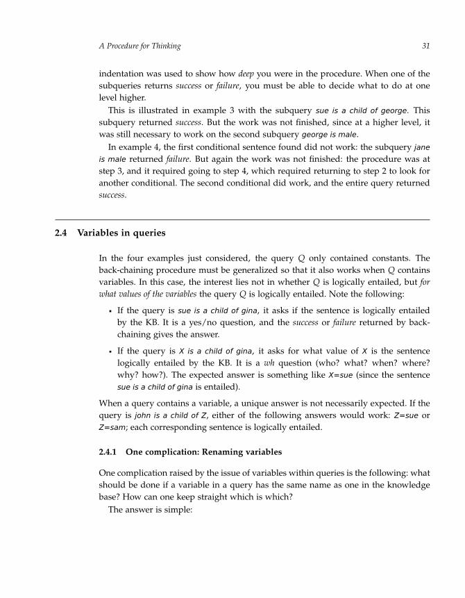
“run” — 2011/9/8 — 18:05 — page 31 — #54�

�

�

�

�

�

�

�


indentation was used to show how deep you were in the procedure. When one of thesubqueries returns success or failure, you must be able to decide what to do at onelevel higher.

This is illustrated in example 3 with the subquery sue is a child of george. Thissubquery returned success. But the work was not finished, since at a higher level, itwas still necessary to work on the second subquery george is male.

In example 4, the first conditional sentence found did not work: the subquery jane

is male returned failure. But again the work was not finished: the procedure was atstep 3, and it required going to step 4, which required returning to step 2 to look foranother conditional. The second conditional did work, and the entire query returnedsuccess.

2.4 Variables in queries

In the four examples just considered, the query Q only contained constants. Theback-chaining procedure must be generalized so that it also works when Q containsvariables. In this case, the interest lies not in whether Q is logically entailed, but forwhat values of the variables the query Q is logically entailed. Note the following:

If the query is sue is a child of gina, it asks if the sentence is logically entailedby the KB. It is a yes/no question, and the success or failure returned by back-chaining gives the answer.

If the query is X is a child of gina, it asks for what value of X is the sentencelogically entailed by the KB. It is a wh question (who? what? when? where?why? how?). The expected answer is something like X=sue (since the sentencesue is a child of gina is entailed).

When a query contains a variable, a unique answer is not necessarily expected. If thequery is john is a child of Z, either of the following answers would work: Z=sue orZ=sam; each corresponding sentence is logically entailed.

2.4.1 One complication: Renaming variables

One complication raised by the issue of variables within queries is the following: whatshould be done if a variable in a query has the same name as one in the knowledgebase? How can one keep straight which is which?

The answer is simple:

“run” — 2011/9/8 — 18:05 — page 32 — #55�

�

�

�

�

�

�

�

Chapter 232

The names of the variables in the sentences of the knowledge base do not reallymatter; they can be changed at any time.

For example,


says exactly the same thing as

If U is a child of V then V is a parent of U.

and exactly the same thing as

If Var13 is a child of Var19 then Var19 is a parent of Var13.

All these sentences make precisely the same connection between child and parent.So to keep variables in a query distinct from those used in a KB, the variables in the

KB can be renamed without changing what the sentences are saying. Thus, duringback-chaining, whenever there is a query with variables, the variables in the sentencesof the KB will be renamed to ensure that they differ from the ones in the query. (Theycould be renamed in the query instead, but this is not done here.)

To see this renaming in action, consider the trace shown in figure 2.3 for the querygeorge is a father of Y. Let us review the steps:

1. There is nothing in the KB that matches this query.

2. There is a conditional to consider. However, the names of its variables conflictwith Y in the query, so first change them to U and V. After this renaming, thereis a match as before with U=Y and V=george.

3. After U and V are replaced by their matching values, there are two subqueriesremaining: Y is a child of george and george is male. Note that after replacing thevariables by their matching values, there is still the variable Y to deal with.

1. Look for Y is a child of george in the KB. The KB does not contain this sentenceliterally. But it does contain a matching sentence, from which Y gets the valuesue. So this query succeeds with Y=sue.

2. The query george is male then succeeds straightforwardly.

Since both of these queries succeed, the query george is a father of Y succeedswith Y=sue. This means that george is a father of sue has been established and islogically entailed by the KB.

“run” — 2011/9/8 — 18:05 — page 33 — #56�

�

�

�

�

�

�

�


Figure 2.3. A trace of a query with a variable

Establish the query george is a father of Y.

1. Look for george is a father of Y in the KB. Nothing found.

2. Look for If . . . then george is a father of Y in the KB.Found: If U is a child of V and V is male then V is a father of U.

This matches for V=george and U=Y.


Establish the query Y is a child of george.

1. Look for Y is a child of george in the KB.Found: sue is a child of george, which matches for Y=sue.Return success for Y is a child of george with Y=sue.

Establish the query george is male.


Since both parts were successful, return success for the querygeorge is a father of Y with Y=sue.

2.4.2 Another complication: Backtracking

Another complication can arise with variables in queries because there can be morethan one answer. It is possible that one answer is found, but that later in the back-chaining procedure, the answer leads to failure. In this case, one must go back towhere the answer was found, and see if there is another answer to use in its place.This is called backtracking and is best illustrated using an example.

Consider the query P is a father of john. The search is for someone whom Johnis a child of and who is male, which is to say, Sam. How is the query handled byback-chaining? A trace for it starts as follows:

1. Look for P is a father of john in the KB. Nothing found.

2. Look for If . . . then P is a father of john in the KB.Found: If X is a child of Y and Y is male then Y is a father of X.

This matches for X=john and Y=P.


“run” — 2011/9/8 — 18:05 — page 34 — #57�

�

�

�

�

�

�

�

Chapter 234

Establish the query john is a child of P.

1. Look for john is a child of P in the KB.Found: john is a child of sue, which matches for P=sue.Return success for john is a child of P with P=sue.

Establish the query sue is male.

Let us stop here and review what has happened so far. The query john is a child of P

succeeded. But the first answer found, looking from top to bottom in the KB, was sue.This answer is going to be a problem later: the subquery P is male with P=sue willfail. If there were no backtracking, the whole query would fail. So after discoveringthat the subquery sue is male fails, the back-chaining procedure must backtrack to thesubquery john is a child of P and look for other possibilities. The value sam for P willthen be found, and the rest of the query will eventually succeed.

So just as step 4 of the back-chaining procedure requires going back to step 2 andconsidering other options if things do not work out for the Pi subqueries, backtrackingrequires going back and reconsidering the choice of values for variables if things donot work out.

It is possible to redesign the back-chaining procedure in figure 2.2 to make thisbacktracking explicit, but this is not done here. (The back-chaining procedure shownin figure 3.12 does take this complication into account.) Suffice it to say that theprocedure searches the KB for a matching atomic or conditional sentence, from top tobottom and from left to right, and returns the first match found. But it must be ableto search for other matches if the first match causes problems later.

2.4.3 A more complex query

Let us now consider a more complex query: george is a grandfather of john. The traceis shown in figure 2.4. Although this query does not itself include variables, variablesare introduced for subqueries along the way. For example, a matching conditional instep 2 gives us a value for the variables X and Z but leaves the Y unspecified. This iswhy in the next step there is a subquery with a variable: george is a father of Y. Soeven if a top-level query has no variables, back-chaining would still need to handlesubqueries with variables.

Next, in step 3 of figure 2.4, there are two subqueries: george is a father of Y and Y is

a parent of john. The first one was traced in figure 2.3 and succeeds with Y=sue. (Thisis a good value, and no backtracking will be needed.)

“run” — 2011/9/8 — 18:05 — page 35 — #58�

�

�

�

�

�

�

�


Figure 2.4. A trace of a complex query

Establish the query george is a grandfather of john.

1. Look for george is a grandfather of john in the KB. Nothing found.

2. Look for If . . . then george is a grandfather of john in the KB.Found: If X is a father of Y and Y is a parent of Z then X is a grandfather of Z.

This matches for X=george and Z=john.


Establish the query george is a father of Y.

See the detailed trace in figure 2.3.Return success for george is a father of Y with Y=sue.

Establish the query sue is a parent of john.

1. Look for sue is a parent of john in the KB. Nothing found.

2. Look for If . . . then sue is a parent of john in the KB.Found: If X is a child of Y then Y is a parent of X.

This matches for Y=sue and X=john.

3. Work on the single if-part of the matching conditional:

Establish the query john is a child of sue.1. Look for john is a child of sue in the KB. Found.

Return success for john is a child of sue.

Since this one part was successful, return success for the querysue is a parent of john.

Since both parts were successful, return success for the top-level querygeorge is a grandfather of john.

So for the second subquery in figure 2.4, Y is a parent of john, the Y already has avalue, sue. That is why the second subquery to establish is sue is a parent of john, withno variables remaining. The rest of the trace is similar to previous ones.

This was a complex enough query that it is worth reviewing the thinking that wentinto it in a less formal way:

For George to be a grandfather of John, George needs to be a father of somebodywho is a parent of John.

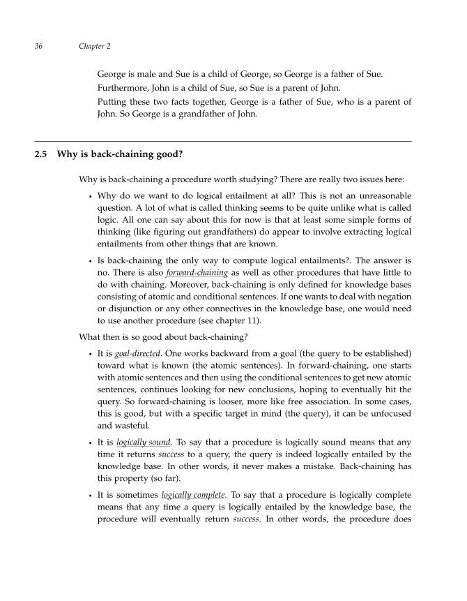
“run” — 2011/9/8 — 18:05 — page 36 — #59�

�

�

�

�

�

�

�

Chapter 236

George is male and Sue is a child of George, so George is a father of Sue.

Furthermore, John is a child of Sue, so Sue is a parent of John.

Putting these two facts together, George is a father of Sue, who is a parent ofJohn. So George is a grandfather of John.

2.5 Why is back-chaining good?

Why is back-chaining a procedure worth studying? There are really two issues here:

Why do we want to do logical entailment at all? This is not an unreasonablequestion. A lot of what is called thinking seems to be quite unlike what is calledlogic. All one can say about this for now is that at least some simple forms ofthinking (like figuring out grandfathers) do appear to involve extracting logicalentailments from other things that are known.

Is back-chaining the only way to compute logical entailments?. The answer isno. There is also forward-chaining as well as other procedures that have little todo with chaining. Moreover, back-chaining is only defined for knowledge basesconsisting of atomic and conditional sentences. If one wants to deal with negationor disjunction or any other connectives in the knowledge base, one would needto use another procedure (see chapter 11).

What then is so good about back-chaining?

It is goal-directed. One works backward from a goal (the query to be established)toward what is known (the atomic sentences). In forward-chaining, one startswith atomic sentences and then using the conditional sentences to get new atomicsentences, continues looking for new conclusions, hoping to eventually hit thequery. So forward-chaining is looser, more like free association. In some cases,this is good, but with a specific target in mind (the query), it can be unfocusedand wasteful.

It is logically sound. To say that a procedure is logically sound means that anytime it returns success to a query, the query is indeed logically entailed by theknowledge base. In other words, it never makes a mistake. Back-chaining hasthis property (so far).

It is sometimes logically complete. To say that a procedure is logically completemeans that any time a query is logically entailed by the knowledge base, theprocedure will eventually return success. In other words, the procedure does

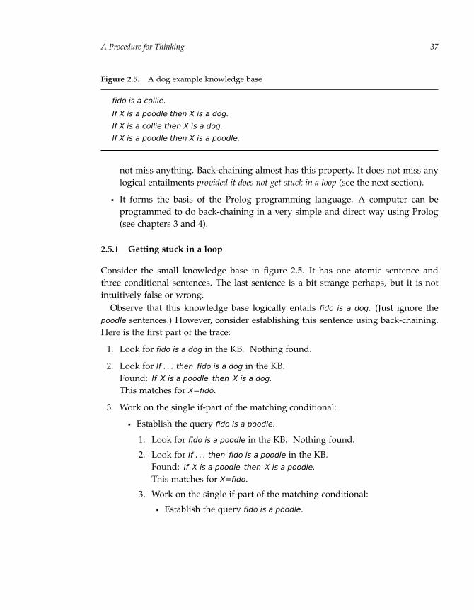
“run” — 2011/9/8 — 18:05 — page 37 — #60�

�

�

�

�

�

�

�


Figure 2.5. A dog example knowledge base

fido is a collie.

If X is a poodle then X is a dog.

If X is a collie then X is a dog.

If X is a poodle then X is a poodle.

not miss anything. Back-chaining almost has this property. It does not miss anylogical entailments provided it does not get stuck in a loop (see the next section).

It forms the basis of the Prolog programming language. A computer can beprogrammed to do back-chaining in a very simple and direct way using Prolog(see chapters 3 and 4).

2.5.1 Getting stuck in a loop

Consider the small knowledge base in figure 2.5. It has one atomic sentence andthree conditional sentences. The last sentence is a bit strange perhaps, but it is notintuitively false or wrong.

Observe that this knowledge base logically entails fido is a dog. (Just ignore thepoodle sentences.) However, consider establishing this sentence using back-chaining.Here is the first part of the trace:

1. Look for fido is a dog in the KB. Nothing found.

2. Look for If . . . then fido is a dog in the KB.Found: If X is a poodle then X is a dog.

This matches for X=fido.


Establish the query fido is a poodle.

1. Look for fido is a poodle in the KB. Nothing found.

2. Look for If . . . then fido is a poodle in the KB.Found: If X is a poodle then X is a poodle.

This matches for X=fido.


Establish the query fido is a poodle.

“run” — 2011/9/8 — 18:05 — page 38 — #61�

�

�

�

�

�

�

�

Chapter 238

It is clear that there is a problem here. In trying to establish fido is a dog, the firstthing the procedure tries is to establish fido is a poodle. Not unreasonable. But insteadof the subquery’s failing (as it should so that collie can be tried next), the procedurefinds the last sentence in the knowledge base and tries fido is a poodle again as asubquery. It is stuck in a loop. It keeps trying to establish fido is a poodle over andover. Consequently, the back-chaining continues forever and never returns success asit should. Therefore, back-chaining is not logically complete.

What caused the problem here was the odd sentence saying that anything that is apoodle is a poodle. Even though the sentence is true, it does not add anything to theknowledge base. (The technical term is that the sentence is a tautology.) So one mightsay that this odd sentence should never have been included in the KB and that back-chaining is not to blame for the procedure’s getting stuck. This is not an unreasonableposition. However, back-chaining can also get stuck on sentences that are not quite soodd, so care will be needed to avoid this undesirable behavior.

Want to read more?

This chapter looked at a computational procedure whose inputs were sentences andwhose output was success or failure, according to whether an input sentence, called thequery, was logically entailed by a separate collection of sentences, called the knowl-edge base. It is a simple matter to get a computer to perform this logical computationin Prolog (see chapter 3).

Logic itself has a long history that in Western culture goes back to the ancientGreeks. The modern form of symbolic logic is due to Gottlob Frege, with a specificnotation due to Giuseppe Peano, in the early 1900s. The motivation for this devel-opment was the desire to put all of mathematical reasoning on a sound footing. Inthe mid 1930s, Kurt Godel was able to prove in his celebrated Incompleteness Theo-rem that this project was doomed, and that mathematical truth (in fact, even simplearithmetic) had to go beyond the application of formal logical rules.

Godel was a genius. But his work, like that of his good friend Albert Einstein,is perhaps outside the reach of beginners. Fortunately, there is a wonderful reviewof this part of the history of logic in comic book form [13] that anyone can readand enjoy. (Introductory textbooks on modern symbolic logic do exist, including atleast two outstanding ones [14, 15], but they necessarily assume some facility withmathematics.)

“run” — 2011/9/8 — 18:05 — page 39 — #62�

�

�

�

�

�

�

�


Although there are many different ways of looking at logic, the focus in this bookis on logical entailment, which in turn depends on thinking about sentences as beingtrue or false. Before 1920 or so, it was typical to think of logic only in terms of axiomsand rules of inference for moving in a correct way from premises to conclusions in argu-ments or proofs. (This would be like studying the properties of back-chaining with nomention of entailment.) Logicians at the time certainly had an intuitive understand-ing of what it meant for a sentence to be true, and they felt confident that the rulesthat they were using were correct (logically sound). But it was only in the late 1920s,spurred by the mathematicians David Hilbert and Wilhelm Ackermann, that theybegan to consider whether the rules they were using were really sufficient (logicallycomplete). In fact, before Godel proved his Incompleteness Theorem, he proved thecompleteness of a certain set of axioms and rules of inference, as part of his doctoralthesis.

Soon thereafter, the logician Alfred Tarski took on the topic of truth. He was thefirst to present a mathematically rigorous definition of a sentence’s being true accord-ing to a precisely laid-out notion of logical interpretation. Logical entailment (or logicalconsequence) could then be given a mathematical account: it held when a conclusionwas true in all interpretations where the premises were true. Tarski’s work revolu-tionized logic, and these days it is rare to see a textbook on symbolic logic that doesnot present the two views of the subject: a syntactic side involving axioms and rulesof inference (sometimes called a proof theory), and a semantic side involving inter-pretations and truth (sometimes called a model theory), with logical soundness andcompleteness theorems relating the two.

The idea of restricting language to atomic and conditional sentences goes backto the logician Alfred Horn, who, on a suggestion from Tarski, first examined theproperties of sentences like these in the early 1950s. They are usually called Hornclauses in his honor, and I use them throughout the book until chapter 11, when Ienlarge the representation language.

Exercises

Consider the knowledge base in figure 2.6 about the east-west subway stops in amythical city somewhere. Note that left of is used here to mean directly to the left of(as it might appear on a subway map).

1. Give an example of an atomic sentence that is not in the knowledge base infigure 2.6 but that is entailed by it.

“run” — 2011/9/8 — 18:05 — page 40 — #63�

�

�

�

�

�

�

�

Chapter 240

Figure 2.6. A subway knowledge base

bay is left of yonge. st-george is left of bay.

spadina is left of st-george. bathurst is left of spadina.

christie is left of bathurst.

If X is left of Y then X is west of Y.

If X is left of Y and Y is west of Z then X is west of Z.

If X is west of Y then Y is east of X.

2. Explain informally why the sentence spadina is right of bathurst is not entailed bythe knowledge base.

3. Trace the back-chaining procedure on the following queries:

a. spadina is west of st-george;

b. yonge is east of bay;

c. christie is west of spadina;

d. yonge is west of yonge;

e. st-george is east of bathurst;

f. bay is west of sherbourne.

4. Suppose the second conditional sentence in the knowledge base is replaced by

If X is west of Y and Y is left of Z then X is west of Z.

Would this change what is entailed? What happens now with the back-chainingprocedure on the query (3d) yonge is west of yonge?

5. Suppose the (incorrect) atomic sentence

yonge is left of bay.

were added to the original knowledge base. For what values of X would theresulting knowledge base entail spadina is west of X? What happens now withthe back-chaining procedure on the query (3f) bay is west of sherbourne?

“run” — 2011/9/8 — 18:05 — page 41 — #64�

�

�

�

�

�

�

�

3 The Prolog Language

The previous chapter showed how a procedure called back-chaining could draw logi-cal conclusions from atomic and conditional sentences. It was the first demonstrationof how a simple form of thinking could be seen as computation. But so far thiscomputation has not involved computers.

This chapter and the next explain how to write computer programs in a languagecalled Prolog. These programs will end up being knowledge bases like those inchapter 2, but formulated in a new way. Queries will direct a computer to performback-chaining, just as was done “by hand” in the previous chapter. If nothing else,this will confirm that thinking, as presented in this book, really is a procedure thatcan be carried out purely mechanically.

Prolog, which stands for programming in logic, is a language for writing programsthat was developed by Alain Colmerauer and colleagues. There are several dialectsof Prolog with minor notational differences. This book uses a popular one calledSWI-Prolog. (See appendix D for details on this and other dialects of Prolog.)

Learning a programming language like Prolog is a bit like learning a foreign lan-guage. It is painstaking and often tedious to memorize not just the new vocabularybut all the rules and regulations of the new language.

Consider a French-speaking person learning English. There will be rules of spellingto learn (like “use ’i’ before ’e’ except after ’c’”), and many more involving grammar.To take just one example, consider talking about the parent of a child. In French, onechooses between the possessive adjectives son and sa depending on whether the parentin question is male or female: sa mere (mother), son pere (father). In English, on theother hand, one learns that the choice of possessive adjective depends on whether thechild in question is male or female: for a boy, it’s his mother, his father; for a girl, it’sher mother, her father.

There is good news and bad news about learning Prolog. The good news is thatthere are only a few rules to be memorized to get all the spelling and grammar ofProlog right. A complete description of the language fits on one page (see figure 3.10).

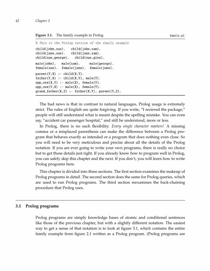
“run” — 2011/9/8 — 18:05 — page 42 — #65�

�

�

�

�

�

�

�

Chapter 342

Figure 3.1. The family example in Prolog family.pl

% This is the Prolog version of the family example

child(john,sue). child(john,sam).

child(jane,sue). child(jane,sam).

child(sue,george). child(sue,gina).

male(john). male(sam). male(george).

female(sue). female(jane). female(june).

parent(Y,X) :- child(X,Y).

father(Y,X) :- child(X,Y), male(Y).

opp_sex(X,Y) :- male(X), female(Y).

opp_sex(Y,X) :- male(X), female(Y).

grand_father(X,Z) :- father(X,Y), parent(Y,Z).

The bad news is that in contrast to natural languages, Prolog usage is extremelystrict. The rules of English are quite forgiving. If you write, “I recieved the package,”people will still understand what is meant despite the spelling mistake. You can evensay, “accident car passenger hospital,” and still be understood, more or less.

In Prolog, there is no such flexibility. Every single character matters! A missingcomma or a misplaced parenthesis can make the difference between a Prolog pro-gram that behaves exactly as intended or a program that does nothing even close. Soyou will need to be very meticulous and precise about all the details of the Prolognotation. If you are ever going to write your own programs, there is really no choicebut to get those details just right. If you already know how to program well in Prolog,you can safely skip this chapter and the next. If you don’t, you will learn how to writeProlog programs here.

This chapter is divided into three sections. The first section examines the makeup ofProlog programs in detail. The second section does the same for Prolog queries, whichare used to run Prolog programs. The third section reexamines the back-chainingprocedure that Prolog uses.

3.1 Prolog programs

Prolog programs are simply knowledge bases of atomic and conditional sentenceslike those of the previous chapter, but with a slightly different notation. The easiestway to get a sense of that notation is to look at figure 3.1, which contains the entirefamily example from figure 2.1 written as a Prolog program. (Prolog programs are

“run” — 2011/9/8 — 18:05 — page 43 — #66�

�

�

�

�

�

�

�

The Prolog Language 43

shown in this font.) To write your own Prolog programs, you will need to knowwhat is and is not allowed. So all the pieces are discussed in detail, starting with thesmallest ones.

Constants

A Prolog constant must start with a lowercase letter and can be followed by any num-ber of letters, underscores, or digits. A constant may also be a quoted-string: any stringof characters (other than a single quote) enclosed within single quotes. The followingare all legal constants:

george grand_father mamboNumber5 ’Who are you?’

Variables

A Prolog variable must start with an uppercase letter and can be followed by anynumber of letters, underscores, or digits. The following are all legal variables:

X P12 MyDog The_biggest_number Parameter_26b

Prolog has other sorts of terms (numbers and lists) and other types of variables(beginning with an underscore), which are discussed later.

Atomic sentences

The Prolog atomic sentences have the following form:

predicate(argument1, . . . , argumentk)

where the predicate is a Prolog constant and the subsequent arguments are either Prologconstants or variables. So, for example,

child(john,X) delivers_package(’Fed Ex’,Sender,Receiver)

are both atomic sentences, whereas

Rich(jim) likes(george,father(bill))

are not. (The first one has a variable in the predicate position, and the second onehas an argument that is not a constant or a variable.) Atomic sentences are sometimescalled atoms for short. Note that instead of john is a child of X, there is a pared-downversion child(john,X), which omits many of the words used in the sentences inchapter 2, puts the predicate at the front, and requires special punctuation:

Immediately after the predicate, there must be a left parenthesis.

‘‘run’’ --- 2011/9/8 --- 18:05 --- page 44 --- #67�

�

�

�

�

�

�

�

Chapter 344

Between each argument, there must be a comma.

Immediately after the last argument, there must be a right parenthesis.

When a predicate has no arguments (k = 0), the parentheses can be left out.

Conditional sentences

The conditional sentences of Prolog have this form:

head :- body1, . . . , bodyn

where the head and each element of the body is a Prolog atom. In this case, thenotation is quite different from the sentences in chapter 2. For one thing, the head,which represents the then part, appears first, and the body, which represents the if

part, appears afterward. So

father(Y,X) :- child(X,Y), male(Y)

is equivalent to If X is a child of Y and Y is male then Y is a father of X. Note that thewords if, then, and and are left out, and special punctuation is required:

Immediately after the head, there must be a colon and then a hyphen.

Between each element of the body, there must be a comma.

When the body is empty (n = 0), the :- should be omitted. This means that as faras Prolog is concerned, an atomic sentence is really just a special case of a conditionalsentence where the body happens to be empty. (The body can also include otherthings discussed later.)

In sum, a Prolog program is a sequence of clauses, where a clause is an atomicor conditional sentence terminated by a period. To make programs easier to read(without changing what the program does), spaces, newlines, and comments canbe inserted at the end of a program or just before a constant or variable. A Prologcomment starts with a % character (the percent sign) and continues to the end of theline. (In this book, comments are shown in gray italics, but they do not have to be.Only the percent sign is required.)

Here is a very short but complete Prolog program:

zzz.

This is a Prolog program for the following reasons. A program can be a single clauseterminated by a period; a clause can be an atomic sentence; an atomic sentence canbe a predicate with no arguments or parentheses; a predicate is written as a constant;and finally, zzz is a constant. Here is a somewhat longer program:

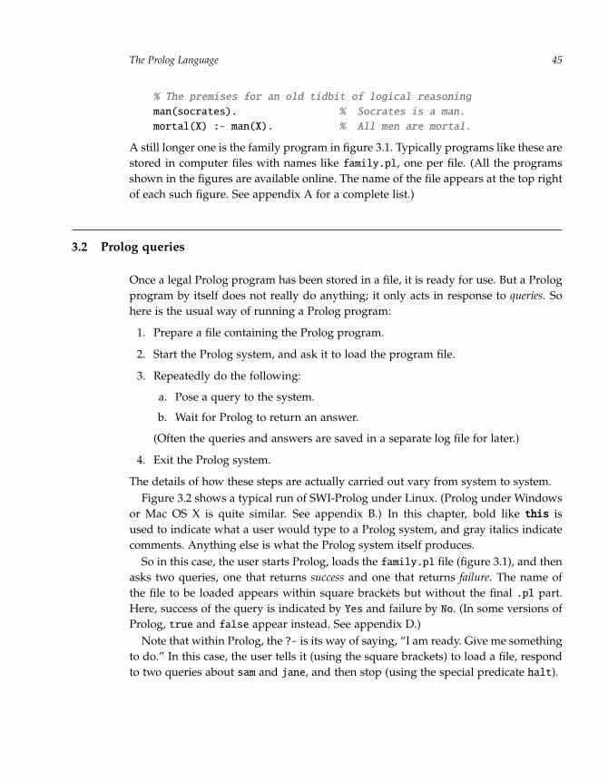
“run” — 2011/9/8 — 18:05 — page 45 — #68�

�

�

�

�

�

�

�


% The premises for an old tidbit of logical reasoning

man(socrates). % Socrates is a man.

mortal(X) :- man(X). % All men are mortal.

A still longer one is the family program in figure 3.1. Typically programs like these arestored in computer files with names like family.pl, one per file. (All the programsshown in the figures are available online. The name of the file appears at the top rightof each such figure. See appendix A for a complete list.)

3.2 Prolog queries

Once a legal Prolog program has been stored in a file, it is ready for use. But a Prologprogram by itself does not really do anything; it only acts in response to queries. Sohere is the usual way of running a Prolog program:

1. Prepare a file containing the Prolog program.

2. Start the Prolog system, and ask it to load the program file.

3. Repeatedly do the following:

a. Pose a query to the system.

b. Wait for Prolog to return an answer.

(Often the queries and answers are saved in a separate log file for later.)

4. Exit the Prolog system.

The details of how these steps are actually carried out vary from system to system.Figure 3.2 shows a typical run of SWI-Prolog under Linux. (Prolog under Windows

or Mac OS X is quite similar. See appendix B.) In this chapter, bold like this isused to indicate what a user would type to a Prolog system, and gray italics indicatecomments. Anything else is what the Prolog system itself produces.

So in this case, the user starts Prolog, loads the family.pl file (figure 3.1), and thenasks two queries, one that returns success and one that returns failure. The name ofthe file to be loaded appears within square brackets but without the final .pl part.Here, success of the query is indicated by Yes and failure by No. (In some versions ofProlog, true and false appear instead. See appendix D.)

Note that within Prolog, the ?- is its way of saying, “I am ready. Give me somethingto do.” In this case, the user tells it (using the square brackets) to load a file, respondto two queries about sam and jane, and then stop (using the special predicate halt).

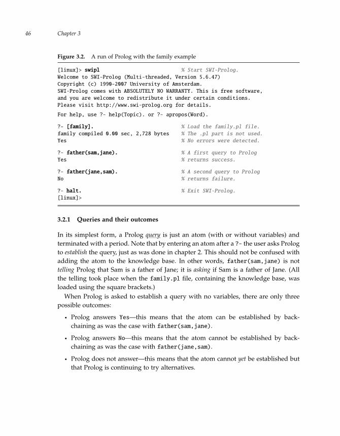
“run” — 2011/9/8 — 18:05 — page 46 — #69�

�

�

�

�

�

�

�

Chapter 346

Figure 3.2. A run of Prolog with the family example

[linux]> swipl % Start SWI-Prolog.

Welcome to SWI-Prolog (Multi-threaded, Version 5.6.47)

Copyright (c) 1990-2007 University of Amsterdam.

SWI-Prolog comes with ABSOLUTELY NO WARRANTY. This is free software,

and you are welcome to redistribute it under certain conditions.

Please visit http://www.swi-prolog.org for details.

For help, use ?- help(Topic). or ?- apropos(Word).

?- [family]. % Load the family.pl file.

family compiled 0.00 sec, 2,728 bytes % The .pl part is not used.

Yes % No errors were detected.

?- father(sam,jane). % A first query to Prolog

Yes % returns success.

?- father(jane,sam). % A second query to Prolog

No % returns failure.

?- halt. % Exit SWI-Prolog.

[linux]>

3.2.1 Queries and their outcomes

In its simplest form, a Prolog query is just an atom (with or without variables) andterminated with a period. Note that by entering an atom after a ?- the user asks Prologto establish the query, just as was done in chapter 2. This should not be confused withadding the atom to the knowledge base. In other words, father(sam,jane) is nottelling Prolog that Sam is a father of Jane; it is asking if Sam is a father of Jane. (Allthe telling took place when the family.pl file, containing the knowledge base, wasloaded using the square brackets.)

When Prolog is asked to establish a query with no variables, there are only threepossible outcomes:

Prolog answers Yes—this means that the atom can be established by back-chaining as was the case with father(sam,jane).

Prolog answers No—this means that the atom cannot be established by back-chaining as was the case with father(jane,sam).

Prolog does not answer—this means that the atom cannot yet be established butthat Prolog is continuing to try alternatives.

“run” — 2011/9/8 — 18:05 — page 47 — #70�

�

�

�

�

�

�

�


Figure 3.3. Two more queries after loading the family.pl program

?- father(sam,X). % Who is Sam a father of?

X = john

Yes

?- father(U,V). % Who is a father of whom?

U = sam

V = john ; % Any more?

U = sam

V = jane ; % Any more?

U = george

V = sue ; % Any more?

No

For a query with variables, there will also be three possible outcomes:

Prolog answers No—this means that the atom cannot be established for anyvalues of the variables.

Prolog does not answer—this means that the atom cannot yet be established forany values of the variables but that Prolog is continuing to try alternatives.

Prolog displays values for the variables for which it can establish the query. Atthis point the user has some choices:

– If the user types a space or a return, Prolog answers Yes and the queryanswering is complete.

– If the user types a semicolon (;), Prolog tries to find new values for thevariables, again with the same three possible outcomes.

So if a query with a variable can be established for different values of the variable,these values can be examined one at a time by using the ; command.

To see how this all works, restart Prolog and again load the family.pl program, asin figure 3.2. Then pose some additional queries.

The first query shown in figure 3.3 uses a variable to ask who Sam is a father of.Prolog responds that an answer is John. Then the user typed a space, indicating thathe did not want to see if there were any additional possible answers. The user isfinished with this query.

The second query asks Prolog who is a father of whom using two variables: U forthe father and V for the child. Prolog returns the pair Sam and John (meaning that itcan establish that Sam is a father of John). The user then types a ; asking Prolog to see

“run” — 2011/9/8 — 18:05 — page 48 — #71�

�

�

�

�

�

�

�

Chapter 348

Figure 3.4. Conjunctive queries after loading the family.pl program

?- female(jane), parent(sam,jane).Yes

?- female(F), parent(sam,F).F = jane ;No

if there are any additional answers. It returns Sam and Jane as the next answer. (Samefather, different child.) The user asks for more with another ; and Prolog answersGeorge and Sue. The users asks for more with another ; and it answers No (meaningit is unable to establish the query for any other values).

3.2.2 Conjunctive queries

So far, queries have been single atoms terminated with a period. Prolog also allowsconjunctive queries, which are sequences of atoms separated by commas and terminatedby a period. These queries are understood conjunctively, in the sense that Prolog isasked to establish all the atoms in a single query (from left to right). So the comma ina conjunctive query plays the role of and just as it does in the body of a conditionalsentence.

Assuming the family.pl file is loaded as before, consider the two queries infigure 3.4. The first one asks if Jane is female and if Sam is a parent of Jane. Theanswer is Yes. But this is not very useful, since the job could have been done withtwo separate atomic queries. What makes conjunctive queries useful is when thereare variables that appear in more than one atom. So, for example, in the second queryin figure 3.4, the variable F appears in both parts. This query asks if there is an F thatsatisfies two properties: F is female and Sam is a parent of F. Another way of sayingthis: Is there a female that Sam is a parent of? The key point is that the user seeksthe same person for both atoms. The answer returned by Prolog is Jane, and after theuser types the ; command to ask if there are more, Prolog says No (Jane is the onlyanswer).

Chapter 2 did not deal with conjunctive queries like this, but they were thereimplicitly. The back-chaining procedure (see figure 2.2) contained the following twoinstructions:

2. Otherwise, try to locate a conditional sentence of the formIf P1 and . . . and Pn then Q in the KB. If you cannot, return failure.

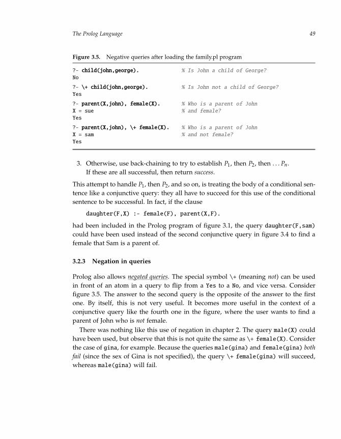
“run” — 2011/9/8 — 18:05 — page 49 — #72�

�

�

�

�

�

�

�


Figure 3.5. Negative queries after loading the family.pl program

?- child(john,george). % Is John a child of George?

No

?- \+ child(john,george). % Is John not a child of George?

Yes

?- parent(X,john), female(X). % Who is a parent of John

X = sue % and female?

Yes

?- parent(X,john), \+ female(X). % Who is a parent of John

X = sam % and not female?

Yes

3. Otherwise, use back-chaining to try to establish P1, then P2, then . . . Pn.If these are all successful, then return success.

This attempt to handle P1, then P2, and so on, is treating the body of a conditional sen-tence like a conjunctive query: they all have to succeed for this use of the conditionalsentence to be successful. In fact, if the clause

daughter(F,X) :- female(F), parent(X,F).

had been included in the Prolog program of figure 3.1, the query daughter(F,sam)could have been used instead of the second conjunctive query in figure 3.4 to find afemale that Sam is a parent of.

3.2.3 Negation in queries

Prolog also allows negated queries. The special symbol \+ (meaning not) can be usedin front of an atom in a query to flip from a Yes to a No, and vice versa. Considerfigure 3.5. The answer to the second query is the opposite of the answer to the firstone. By itself, this is not very useful. It becomes more useful in the context of aconjunctive query like the fourth one in the figure, where the user wants to find aparent of John who is not female.

There was nothing like this use of negation in chapter 2. The query male(X) couldhave been used, but observe that this is not quite the same as \+ female(X). Considerthe case of gina, for example. Because the queries male(gina) and female(gina) bothfail (since the sex of Gina is not specified), the query \+ female(gina) will succeed,whereas male(gina) will fail.

“run” — 2011/9/8 — 18:05 — page 50 — #73�

�

�

�

�

�

�

�

Chapter 350

It is worth observing that if one reads the query \+ female(gina) as saying thatGina is not female, then the conclusions from Prolog are no longer logically sound.Although the query succeeds, it is not the case that the family knowledge baselogically entails that Gina is not female; the sex of Gina is left unspecified.

3.2.4 Tracing the back-chaining

In considering an extended version of back-chaining to handle negation, it isworthwhile to follow how Prolog answers conjunctive queries with negation like

parent(X,john), \+ female(X).

to see how Prolog ends up with the answer X = sam.

1. Start by replacing variables in the query with new names to make sure that theydo not conflict with any variables that appear in the Prolog program:

parent(_G312,john), \+ female(_G312).

2. Work on the first atom in the query, parent(_G312,john). Find the clauseparent(Y,X) :- child(X,Y) in the program (figure 3.1) whose head matchesthe first atom in the query. This leaves the conjunctive query

child(john,_G312), \+ female(_G312).

to work on. (The second part of the query is kept unchanged.)

3. Work on the first atom of the new query, child(john,_G312). Find a matchingclause child(john,sue) with no body in the program (figure 3.1). Tentatively,this part of the query is finished. This leaves the query

\+ female(sue).

(Note that the child(john,sue) clause in the program was a bad choice. It willbe necessary to backtrack, but that is not known yet.)

4. Work on \+ female(sue). Since this is a negated query, remove the \+ andconsider the unnegated version.

a. Work on the query female(sue), and find a matching atomic sentence in theprogram. Return success.

Since the unnegated version succeeds, the negated query fails. Backtrack to themost recent choice point (step 3) and reconsider.

“run” — 2011/9/8 — 18:05 — page 51 — #74�

�

�

�

�

�

�

�


Figure 3.6. A Prolog trace for a query

?- parent(X,john), \+ female(X).Call: (8) parent(_G312,john)

Call: (9) child(john,_G312)

Exit: (9) child(john,sue)

Exit: (8) parent(sue,john)

Call: (8) female(sue)

Exit: (8) female(sue)

Redo: (9) child(john,_G312)

Exit: (9) child(john,sam)

Exit: (8) parent(sam,john)

Call: (8) female(sam)

Fail: (8) female(sam)

X = sam

Yes

5. Reconsider the atom child(john,_G312) (from step 3). Find the next matchingclause, child(john,sam) with no body in the program. Tentatively, this part ofthe query is finished. This leaves

\+ female(sam).

6. Work on \+ female(sam). Since this is a negated query, remove the \+ andconsider the unnegated version.

a. Work on the query female(sam). There is no clause in the program whosehead matches this query. Return failure.

Since the unnegated version fails, the negated query succeeds.

7. Since there is nothing left in the conjunctive query, return success, noting thatthe value of X is sam.

One very nice feature of most Prolog systems is that one can ask Prolog itself todo the tracing. This is very helpful when there is a Prolog program that is legal, butwhere some queries do not yield hoped-for results.

Figure 3.6 shows an example of a Prolog trace for the same query. (How to turnon and turn off this tracing behavior varies from system to system. See appendix C.)This trace goes through roughly the same steps as the previous detailed listing. Fourtypes of lines printed:

A line that begins Call: is printed when Prolog starts to work on an atomicquery.

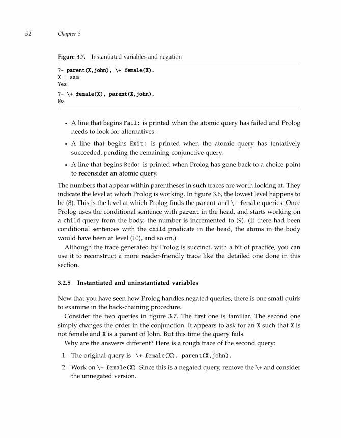
“run” — 2011/9/8 — 18:05 — page 52 — #75�

�

�

�

�

�

�

�

Chapter 352

Figure 3.7. Instantiated variables and negation

?- parent(X,john), \+ female(X).X = sam

Yes

?- \+ female(X), parent(X,john).No

A line that begins Fail: is printed when the atomic query has failed and Prologneeds to look for alternatives.

A line that begins Exit: is printed when the atomic query has tentativelysucceeded, pending the remaining conjunctive query.

A line that begins Redo: is printed when Prolog has gone back to a choice pointto reconsider an atomic query.

The numbers that appear within parentheses in such traces are worth looking at. Theyindicate the level at which Prolog is working. In figure 3.6, the lowest level happens tobe (8). This is the level at which Prolog finds the parent and \+ female queries. OnceProlog uses the conditional sentence with parent in the head, and starts working ona child query from the body, the number is incremented to (9). (If there had beenconditional sentences with the child predicate in the head, the atoms in the bodywould have been at level (10), and so on.)

Although the trace generated by Prolog is succinct, with a bit of practice, you canuse it to reconstruct a more reader-friendly trace like the detailed one done in thissection.

3.2.5 Instantiated and uninstantiated variables

Now that you have seen how Prolog handles negated queries, there is one small quirkto examine in the back-chaining procedure.

Consider the two queries in figure 3.7. The first one is familiar. The second onesimply changes the order in the conjunction. It appears to ask for an X such that X isnot female and X is a parent of John. But this time the query fails.

Why are the answers different? Here is a rough trace of the second query:

1. The original query is \+ female(X), parent(X,john).

2. Work on \+ female(X). Since this is a negated query, remove the \+ and considerthe unnegated version.

“run” — 2011/9/8 — 18:05 — page 53 — #76�

�

�

�

�

�

�

�


a. Work on the query female(X); this query succeeds. (The value of X will notmatter.)

Since the unnegated version succeeds, \+ female(X) fails. The back-chainingdoes not go on to the second atom; it simply returns failure.

So the second query fails because its first part, \+ female(X), fails. And that failsbecause its unnegated version, female(X), succeeds. So the trace never makes it tothe step “and X is a parent of John.”

The difference between the two queries is this. In the second query, the variableX is uninstantiated (does not yet have a tentative value) when the negated portion ofthe query is handled. In the first query, the variable X is instantiated (has a tentativevalue) before the negation step. Back-chaining with negation handles these two casesdifferently.

While there may be cases when something like the second query is wanted, theywill be very rare. One is much more likely to want to know about the nonfemaleparents of John (and to require something like the first query).

When variables appear in a negated query, make sure that they are alreadyinstantiated at an earlier stage of the back-chaining.

The most common way to ensure that a variable is instantiated is by using anotheratom in a query before the negated part, as is done in the first query of figure 3.7.

3.2.6 Equality in queries

The final refinement to the language of queries concerns equality queries. Prolog allowselements in a query of the form

term1 = term2

where the two terms are either constants or variables. This query succeeds when thetwo terms can be made equal by instantiating any variables, and fails otherwise. Someexamples are presented in figure 3.8.

The first and second queries succeed by instantiating both X and Y to sam. The thirdquery fails, since there is no way to instantiate X and Y to satisfy all three requirements.Finally, in the last query, there is a new form of answer to a query with variables: thequery succeeds but there is no single constant value for X and Y. Prolog indicates thisby putting a variable as the value for X and for Y. The fact that the same variable is usedfor both X and Y is Prolog’s way of saying that they can be instantiated to anything,but the two values must be the same.

“run” — 2011/9/8 — 18:05 — page 54 — #77�

�

�

�

�

�

�

�

Chapter 354

Figure 3.8. Queries using equality

?- X=sam, X=Y.X = sam

Y = sam

Yes

?- X=Y, sam=X, \+ Y=jack.X = sam

Y = sam

Yes

?- X=Y, sam=X, \+ Y=sam.No

?- X=Y.X = _G180

Y = _G180

Yes

As it turns out, inequality is more useful than equality in queries. In fact, it is nevernecessary to use unnegated equality in a query. Instead of writing a query like

child(john,X), child(jane,Y), X=Y.

one should write

child(john,X), child(jane,X).

where the same variable is used more than once. However, negated equality doescome in handy, as seen in the queries of figure 3.9.

The first query asks if Sam is parent of someone other than John. In the back-chaining required for this query, X will be instantiated by the parent query and thefirst tentative value happens to be john. The negated equality fails for this value, andso the parent query is reconsidered, and the second tentative value, jane, is found,for which the rest of the query succeeds.

The second query is the first attempt to get the names of three males. Observe thatthis does not work properly, since all three variables can have the same value. Thethird query remedies this and insists that the three values must not be equal, usingnegated equalities. In this case, Prolog reconsiders the male queries and comes upwith three distinct values, john, sam, and george.

“run” — 2011/9/8 — 18:05 — page 55 — #78�

�

�

�

�

�

�

�


Figure 3.9. Queries using negated equality

?- parent(sam,X), \+ X=john.X = jane

Yes

?- male(X), male(Y), male(Z).X = john

Y = john

Z = john

Yes

?- male(X), male(Y), male(Z), \+ X=Y, \+ X=Z, \+ Y=Z.X = john

Y = sam

Z = george

Yes

A review of programs and queries

Figure 3.10 reviews progress so far, with a few minor extensions. First, the wordterm is introduced to mean a constant, variable, or number, and the word literal tomean a possibly negated atom or equality. More significantly, the notion of a clauseis extended so that the body can be any query. So equalities and negations can now bepart of the body of a clause. These will be handled during back-chaining exactly asthey would be if they were part of a conjunctive query. For example, a clause like

has_two_children(X) :- child(Y1,X), child(Y2,X), \+ Y1=Y2.

can be in a program as a way of defining a new predicate has_two_children thatholds when a person X has (at least) two children. (Without the \+ Y1=Y2 literal, theY1 and Y2 could be the same child.)

3.3 Prolog back-chaining

This section examines in more detail the back-chaining procedure introduced inchapter 2 to characterize exactly how Prolog goes about using a program that hasbeen loaded to establish a query. Figure 3.11 shows a new, simpler example programcalled likes.pl.

“run” — 2011/9/8 — 18:05 — page 56 — #79�

�

�

�

�

�

�

�

Chapter 356

Figure 3.10. A review of Prolog programs and queries

Here are the pieces that make up Prolog programs and queries:

A constant is either a string of characters enclosed within single quotes or alowercase letter optionally followed by letters, digits, and underscores.

A variable is an uppercase letter or an underscore optionally followed by letters,digits, and underscores.

A number is a sequence of one or more digits optionally preceded by a minussign and optionally containing a decimal point.

A term is a constant, variable, or number.

A predicate is written as a constant.

An atom is a predicate optionally followed by terms (called the arguments of thepredicate) enclosed within parentheses and separated by commas.

An equality is two terms separated by the = symbol.

A literal is an atom or an equality optionally preceded by the \+ symbol.

A query is a sequence of one or more literals separated by commas andterminated with a period.

A clause is an atom (called the head of the clause) followed by a period or by the:- symbol and then a query (called the body of the clause).

A program is a sequence of one or more clauses.

Figure 3.11. The likes example likes.pl

% This is a program about who likes what kinds of food.

likes(john,pizza). % John likes pizza.

likes(john,sushi). % John likes sushi.

likes(mary,sushi). % Mary likes sushi.

likes(paul,X) :- likes(john,X). % Paul likes what John likes.

likes(X,icecream). % Everybody likes ice cream.

3.3.1 Unification

Clauses in a program are selected during back-chaining through a matching processcalled unification. Two atoms whose variables are distinct are said to unify if there is a

“run” — 2011/9/8 — 18:05 — page 57 — #80�

�

�

�

�

�

�

�


substitution of values for the variables that makes the atoms identical. Here are someexamples:

A query such as likes(john,Y) unifies with likes(john,pizza) in the firstclause of the program, for Y=pizza.

A query such as likes(paul,pizza) unifies with likes(paul,X) in the fourthclause of the program, for X=pizza.

A query such as likes(jane,Y) unifies with likes(X,icecream) in the lastclause of the program, for X=jane and Y=icecream.

In all three cases, the given queries would eventually succeed.Note that both the query and the head of a clause from the program may contain

variables. In fact, unification is not concerned with where the atoms come from, whichone is from the query and which one is from the program.

As further examples, the following pairs of atoms will unify:

p(b,X,b) and p(Y,a,b) for X=a and Y=b

p(X,b,X) and p(a,b,Y) for X=a and Y=a

p(b,X,b) and p(Y,Z,b) for X=_G12, Y=b, and Z=_G12(In this case, the substitution that unifies the two atoms is not unique in that, forexample, X=c, Y=b, and Z=c also unifies the two atoms.)

p(X,Z,X,Z) and p(Y,W,a,Y) for X=a, Z=a, Y=a and W=a(In this case, the unifying substitution is unique.)

Here are some examples of pairs of atoms that do not unify:

p(b,X,b) and p(b,Y)(The two terms cannot be made identical, since the predicates have differentnumbers of arguments.)

p(b,X,b) and p(Y,a,a)(The last arguments are constants that clash.)

p(X,b,X) and p(a,a,b)(The two occurrences of X are required to match different constants.)

p(X,b,X,a) and p(Y,Z,Z,Y)(The two occurrences of X force the Y and Z to be equal, but they must also matcha and b, respectively.)

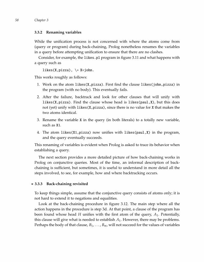
“run” — 2011/9/8 — 18:05 — page 58 — #81�

�

�

�

�

�

�

�

Chapter 358

3.3.2 Renaming variables

While the unification process is not concerned with where the atoms come from(query or program) during back-chaining, Prolog nonetheless renames the variablesin a query before attempting unification to ensure that there are no clashes.

Consider, for example, the likes.pl program in figure 3.11 and what happens witha query such as

likes(X,pizza), \+ X=john.

This works roughly as follows:

1. Work on the atom likes(X,pizza). First find the clause likes(john,pizza) inthe program (with no body). This eventually fails.

2. After the failure, backtrack and look for other clauses that will unify withlikes(X,pizza). Find the clause whose head is likes(paul,X), but this doesnot (yet) unify with likes(X,pizza), since there is no value for X that makes thetwo atoms identical.

3. Rename the variable X in the query (in both literals) to a totally new variable,such as X1.

4. The atom likes(X1,pizza) now unifies with likes(paul,X) in the program,and the query eventually succeeds.

This renaming of variables is evident when Prolog is asked to trace its behavior whenestablishing a query.

The next section provides a more detailed picture of how back-chaining works inProlog on conjunctive queries. Most of the time, an informal description of back-chaining is sufficient, but sometimes, it is useful to understand in more detail all thesteps involved, to see, for example, how and where backtracking occurs.

∗ 3.3.3 Back-chaining revisited

To keep things simple, assume that the conjunctive query consists of atoms only; it isnot hard to extend it to negations and equalities.

Look at the back-chaining procedure in figure 3.12. The main step where all theaction happens in the procedure is step 3d. At that point, a clause of the program hasbeen found whose head H unifies with the first atom of the query, A1. Potentially,this clause will give what is needed to establish A1. However, there may be problems.Perhaps the body of that clause, B1, . . . , Bm, will not succeed for the values of variables

“run” — 2011/9/8 — 18:05 — page 59 — #82�

�

�

�

�

�

�

�


Figure 3.12. The Prolog back-chaining procedure

To establish a query consisting of atoms A1, A2, . . . , An:

1. If n = 0, there’s nothing to do, and so exit with success.

2. Otherwise, begin by renaming all the variables in the conjunctive query.

3. Go through each clause of the program from top to bottom:

a. Assume the current clause has head H and body B1, . . . , Bm, (where foratomic clauses, m = 0).

b. Test to see if the head H unifies with A1, the first atom of the query.

c. If it does not unify, try the next clause in the program.

d. If it does unify, try to establish B∗1 , . . . , B∗

m, A∗2 ,. . . , A∗

n, by back-chaining,where the ∗ means the result of replacing the variables by their values afterunification.

e. If the resulting conjunctive query was successful, exit the procedure withsuccess; if it was not successful, then try the next clause in the program (justas if the H had not unified at step 3c).

4. If all of the clauses of the program have been tried without success, then exitwith failure.

after the unification of H and A1, or perhaps the rest of the query, A2, . . . , An, will notsucceed for the values of variables after that unification, and backtracking is indicated.So even though the H unifies with A1, this may not be the desired clause, and theprocedure will look for alternatives for A1 in step e.

To deal with such issues, back-chaining is invoked on a new conjunctive query,B∗

1 , . . . , B∗m, A∗

2 , . . . , A∗n, where two changes have been made to the original:

A1 has been replaced in the query by the body of the clause whose head matchesA1. Note that if that matching clause had no body (that is, if the clause wasatomic), then there are no Bi atoms, the new query starts at A2, and the first partof the query is finished, at least tentatively.

After unifying A1 with H, the procedure considers the values of the resultingvariables. Some variables might appear in both the head and the body of thematching clause and the procedure needs to have the right values for those vari-ables. Also, there can be variables in A1 that appear in the rest of the conjunctive

“run” — 2011/9/8 — 18:05 — page 60 — #83�

�

�

�

�

�

�

�

Chapter 360

query, and the procedure needs to have the right values for those variables whengoing on to A2.

As mentioned in chapter 2, the back-chaining procedure is recursive. This meansthat part of what it takes to execute the procedure (for certain inputs) involves exe-cuting that same procedure on some other inputs. In this case, part of what it takesto do back-chaining on a query is to do back-chaining on another query. This is whathappens in step 3d.

To establish the query

A1, A2, . . . , An,

the procedure tries to establish the query

B∗1 , B∗

2 , . . . , B∗m, A∗

2 , . . . , A∗n.

How can this possibly work? It might seem that working on this new query, theprocedure would get to step 3d again and find another clause whose head matchesB∗

1 and whose body is C1, . . . , Ck. Does this not go on forever, producing longer andlonger queries?

It might. Back-chaining can get stuck in a loop and never finish.However, in other cases, the query that arises in step 3d will be easier to solve than

the original one. For example, there may be no body at all in the clause that matchesA1, in which case, the procedure goes from a query with n atoms to one with (n − 1)atoms (and eventually to (n − 2), and so on, until it gets to 0). Or perhaps there is abody, but it may be able to deal with B∗

1 directly in one step (when there is a matchingclause that has no body).

At any rate, for back-chaining to return success, it must first deal with A1 by dealingwith any Bi atoms that it finds, which may result in dealing with Ci atoms (andperhaps Di atoms, and so on). When these are all done, then (and only then) doesback-chaining go on to the A2 and the procedure continues (possibly leading to newBi atoms, as before). A3 is dealt with in the same way. Eventually, one of two thingshappens: either the procedure cannot establish one of these Ai no matter what it tries,in which case it returns failure; or the procedure gets through all the Ai and ends upwith the empty conjunctive query, in which case it returns success.

Note that in handling A1, the procedure looks for clauses to use and then tries toestablish a new conjunctive query. If this new query fails, it is not yet done. In fact,it may have failed because the clause it chose for A1 was not a good one. (It may notbe a good one even if it has no body; the unification may require bindings for thevariables in A1 that will not work for A2, say.) So instead of immediately returningfailure after the recursive query fails in step 3d, the procedure backtracks and looks

“run” — 2011/9/8 — 18:05 — page 61 — #84�

�

�

�

�

�

�

�


for another clause to work with A1, in step 3e. It is only when it runs out of clausesto use for A1 that it finally returns failure, in step 4.

Want to read more?

This chapter presented Prolog as a language for writing programs and queries, andshowed how a Prolog system uses back-chaining to answer queries. Chapter 4 dealswith how to write meaningful Prolog programs.

Prolog was developed by Alain Colmerauer at the Universite d’Aix-Marseille II andthe Universite de Montreal in the early 1970s. Philippe Roussel and Robert Kowalskiwere also early contributors. (See [16] for some of the history.) Many of the ideasin Prolog were proposed independently in a slightly different form by Carl Hewitt atthe Massachusetts Institute of Technology in a computer language called Planner [17].Prolog was originally intended for computer programs that process natural languageinputs such as English or French, but it is now used for a wide variety of applications,mainly having to do with artificial intelligence or databases.

Prolog is used most commonly in Britain and France but has enthusiastic fansworldwide. It is often studied as a programming language in computer sciencecourses because it presents a unique view of programming compared to the moreconventional programming languages like C++, Java, or Python.

Exercises

Make up a simple knowledge base of atomic sentences about movies (not necessarilyreal ones) using the following predicates:

acted_in(person,movie) the person acted in the moviedirected(person,movie) the person directed the moviereleased(movie,year) the movie came out that year

You can use numbers like 2011 as constants. You may also find it convenient to usequoted strings like ’The Big Lebowski’ as constants.

Save your knowledge base as a Prolog program in a file, and load it into Prolog.Then pose the following questions as queries to Prolog, and obtain Prolog’s answers:

1. Did Leonardo DiCaprio act in Babel?

2. Who directed District 9?

“run” — 2011/9/8 — 18:05 — page 62 — #85�

�

�

�

�

�

�

�

Chapter 362

3. Did anyone act in both Click and The Aviator?

4. Was there a movie released in 2010 that did not star Jennifer Anniston?

5. Who directed movies released in 2009?

Using the ; command, have Prolog list all such movies and their directors.

6. Has anyone directed more than one movie?

7. Does any movie have more than one director?

8. Has anyone acted in more than one movie released in 2008?

9. Has anyone acted in more than two movies in the same year?

10. Who has worked with the same director in different years?

Using the ; command, have Prolog list all such actors, directors, the movies theyworked on together, and the years the movies were released .

Note: There’s nothing wrong with getting failure answers from Prolog. But to besure you have formulated the queries correctly, you may want to change some of thenames in the queries, or include some additional movies in your knowledge base.

“run” — 2011/9/8 — 18:05 — page 63 — #86�

�

�

�

�

�

�

�

4 Writing Prolog Programs

The previous chapter looked at what it takes for a Prolog program to be grammaticallycorrect and how it is then used to establish queries. But there is more to a languagethan just getting the grammar right. There is an old saying in computer science,abbreviated as GIGO: garbage in, garbage out. This means that if the program givento Prolog is grammatically correct but garbage, Prolog will use it to answer querieswithout complaining, but the answers will also be garbage.

This chapter looks at what it takes to write Prolog programs that are not garbage.The first section examines what it means for a program to be fully correct. Section 2introduces a new program in a blocks world and studies how it was written. Thisleads to a discussion of recursion in section 3, and to its companion, mathematicalinduction, in section 4. Section 5 considers the issue of programs that run forever(see section 2.5.1), and how to avoid writing them. Section 6 looks at a more complexpredicate as it appears in the blocks-world program. Finally, section 7 introduces theissue of program efficiency.

4.1 The truth in Prolog

How do we know whether a grammatically correct program will do what it issupposed to? In Prolog, the answer is perhaps clearer than in other programminglanguages. A Prolog program is a knowledge base made up of clauses. Each of thoseclauses is an encoding of an atomic or conditional sentence. To answer the question,we need to consider the truth of these sentences.

4.1.1 The truth, and nothing but

Let us go back to the family example of figure 3.1, which used the predicate child.As far as Prolog is concerned, that name does not mean anything; it could have beenboojum. But the writers of the program had a definite idea in mind when they wrotechild(john,sue) and that idea is expressed by the English sentence “John is a child

“run” — 2011/9/8 — 18:05 — page 64 — #87�

�

�

�

�

�

�

�

Chapter 464

of Sue.” The programmers put that atom in the program because they believed, orwere willing to assume, that the corresponding English sentence was true. If they hadthought that John was a child of Gina, they would have put child(john,gina) in theprogram instead.

Similarly, the program had the clause

parent(Y,X) :- child(X,Y).

because its creators took the English sentence “If x is a child of y, then y is the parentof x” to be true. If, instead, they had used the clause

parent(X,Y) :- child(X,Y).

Prolog would not have complained; the clause is grammatically correct. The troubleis that the results would say that John is both a child and a parent of Sue. Garbage in,garbage out. So the clause is not correct because the English sentence “If x is a childof y, then x is a parent of y” is not true.

Suppose the following is in the program:

my_predicate(X,Y) :- child(X,Y).

Is the corresponding sentence true? It depends on what my_predicate means. It isalways a good idea to include comments in the program to help anyone reading it(including yourself) to understand what was meant:

% my_predicate(X,Y) holds when X is a child of Y, or vice versa.


Now, at least, it is clear that the corresponding sentence is true.

4.1.2 The whole truth

However, it is not enough to make sure that all the clauses are true. If theprogram includes the clause child(john,sue) but does not include the clausechild(john,sam), it will still not work properly. A query asking if Sam is a par-ent of John will not get a good answer even if all the clauses are true (that is, if thesentences they represent are true). The problem is that part of the truth is missing.

Consider, for example, the two clauses in the family example about opp_sex:


opp_sex(Y,X) :- male(X), female(Y).

Suppose the second one had been left out. On the surface, everything looks fine. Theprogram is grammatically correct (Prolog loads it normally), and every clause in theprogram is true. If one didn’t look too carefully, one might read the single clause

“run” — 2011/9/8 — 18:05 — page 65 — #88�

�

�

�

�

�

�

�

Writing Prolog Programs 65

as, “Two people are of opposite sex if one of them is male and the other is female.”But what the single clause actually says is, “x is of opposite sex from y if x is maleand y is female.” It says nothing about the converse, so that information is missing.This is a very easy thing to overlook. It might only come to light when a query likeopp_sex(jane,sam) does not produce the expected answer.

Consider the my_predicate clause. How can one tell whether there are enoughclauses for it. Again, it depends on what the predicate was intended to mean. Fromthe comment it appears that a second clause is needed:

% my_predicate(X,Y) holds when X is a child of Y, or vice versa.


my_predicate(X,Y) :- child(Y,X).

With that second clause, the program matches what was intended.So a Prolog program must include enough clauses to spell out the whole truth.

There are two additional points to remember:

A program might not contain all possible truths about a matter. The family pro-gram did not include the parents of George, for instance. So some truths mightbe missing, for a variety of good reasons. This must be accepted, and sometimesdocumented with comments.

But a program must include all relevant truths, explicitly or implicitly. Considerthe truth that Sue is a parent of John. Nowhere is the clause parent(sue,john)in the program. The reason is that this clause can be derived from other clausesusing back-chaining; its truth is represented implicitly by the program. So tocapture the whole truth, one needs to allow for the fact that some of it will becalculated by back-chaining over the knowledge base.

In summary, when writing Prolog programs, all the clauses in a Prolog programmust be true, and all the necessary clauses must be represented somehow in theprogram in a way that Prolog can find them using back-chaining.

Writing a Prolog program involves building a knowledge base of clauses thatcaptures1. the truth, and nothing but,

2. the whole truth,

3. in a form suitable for back-chaining.

Saying that a program is logically correct means that it is correct with respect to gram-mar and to truth: it has exactly the right logical entailments. Saying that a program is

“run” — 2011/9/8 — 18:05 — page 66 — #89�

�

�

�

�

�

�

�

Chapter 466

Figure 4.1. A blocks world

B1

B2

B3

B4

B5

B6 B7

simply correct means that it is grammatically correct, logically correct (criteria 1 and2), and in a form suitable for back-chaining (criterion 3).

4.2 A blocks world

Imagine that we would like to draw appropriate conclusions about a scene like theone depicted in figure 4.1 involving toy blocks on a table. The goal is to describe thisscene and get Prolog to determine that

block B3 is above block B5;

block B1 is to the left of block B7;

block B4 is to the right of block B2.

A Prolog program that does this is presented in figure 4.2. (In that figure, the smallline numbers on the right are for reference only. They are not part of Prolog.) Theprogram uses five predicates, whose intended meaning is described in the comments.With respect to the scene in figure 4.1, the program handles the on and just_leftpredicates appropriately, with the six atomic clauses. Similarly, the single clause forthe right predicate is correct assuming that the ones for the left predicate are cor-rect. (The program says that right is the inverse of left, just as parent was theinverse of child.)

“run” — 2011/9/8 — 18:05 — page 67 — #90�

�

�

�

�

�

�

�


Figure 4.2. A blocks-world program blocks.pl

% on(X,Y) means that block X is directly on top of block Y. 1

on(b1,b2). on(b3,b4). on(b4,b5). on(b5,b6). 2

% just left(X,Y) means that blocks X and Y are on the table 4

% and that X is immediately to the left of Y. 5

just_left(b2,b6). just_left(b6,b7). 6

% above(X,Y) means that block X is somewhere above block Y 8

% in the pile where Y occurs. 9

above(X,Y) :- on(X,Y). 10

above(X,Y) :- on(X,Z), above(Z,Y). 11

% left(X,Y) means that block X is somewhere to the left 13

% of block Y but perhaps higher or lower than Y. 14

left(X,Y) :- just_left(X,Y). 15

left(X,Y) :- just_left(X,Z), left(Z,Y). 16

left(X,Y) :- on(X,Z), left(Z,Y). % leftmost is on something. 17

left(X,Y) :- on(Y,Z), left(X,Z). % rightmost is on something. 18

% right(X,Y) is the opposite of left(X,Y). 20

right(Y,X) :- left(X,Y). 21

But what about the above predicate? How do we know that the whole truth andnothing but the truth is included for this one? Consider the sentences represented bythe clauses in lines 10 and 11:

– If x is directly on y, then x is above y.

– If x is directly on z, and z is above y, then x is above y.

Both these sentences are clearly true. But is this all the necessary information?Let us first check that the clauses work on some examples by looking at a trace

of some queries in figure 4.3. (From now on, user-typed queries are no longerhighlighted in bold.)

For the first query, Prolog determines that block B1 is above block B2 because B1is directly on B2.

For the second query, Prolog determines that block B3 is above block B5 becauseB3 is directly on B4, and B4 is above B5. (It determines that B4 is above B5 becauseB4 is directly on B5.)

So in trying to establish the query above(b3,b5), Prolog had to first establishabove(b4,b5). This means that above is a recursive predicate.

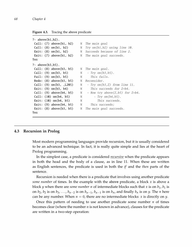
“run” — 2011/9/8 — 18:05 — page 68 — #91�

�

�

�

�

�

�

�

Chapter 468

Figure 4.3. Tracing the above predicate

?- above(b1,b2).

Call: (7) above(b1, b2) % The main goal

Call: (8) on(b1, b2) % Try on(b1,b2) using line 10.

Exit: (8) on(b1, b2) % Succeeds because of line 2.

Exit: (7) above(b1, b2) % The main goal succeeds.

Yes

?- above(b3,b5).

Call: (8) above(b3, b5) % The main goal.

Call: (9) on(b3, b5) % - Try on(b3,b5).

Fail: (9) on(b3, b5) % This fails.

Redo: (8) above(b3, b5) % Reconsider.

Call: (9) on(b3, _L205) % - Try on(b3,Z) from line 11.

Exit: (9) on(b3, b4) % This succeeds for Z=b4.

Call: (9) above(b4, b5) % - Now try above(Z,b5) for Z=b4.

Call: (10) on(b4, b5) % - Try on(b4,b5).

Exit: (10) on(b4, b5) % This succeeds.

Exit: (9) above(b4, b5) % This succeeds;

Exit: (8) above(b3, b5) % The main goal succeeds.

Yes

4.3 Recursion in Prolog

Most modern programming languages provide recursion, but it is usually consideredto be an advanced technique. In fact, it is really quite simple and lies at the heart ofProlog programming.

In the simplest case, a predicate is considered recursive when the predicate appearsin both the head and the body of a clause, as in line 11. When these are writtenas English sentences, the predicate is used in both the if and the then parts of thesentence.

Recursion is needed when there is a predicate that involves using another predicatesome number of times. In the example with the above predicate, a block x is above ablock y when there are some number n of intermediate blocks such that x is on b1, b1 ison b2, b2 is on b3, . . . , bn−2 is on bn−1, bn−1 is on bn, and finally bn is on y. The n herecan be any number. When n = 0, there are no intermediate blocks: x is directly on y.

Once this pattern of needing to use another predicate some number n of timesbecomes clear (where the number n is not known in advance), clauses for the predicateare written in a two-step operation:

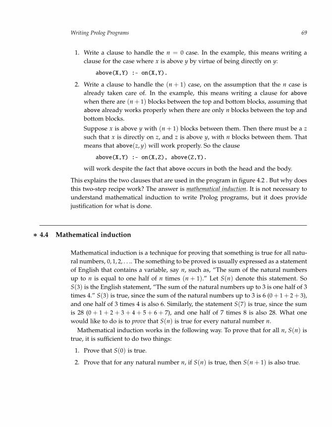
“run” — 2011/9/8 — 18:05 — page 69 — #92�

�

�

�

�

�

�

�


1. Write a clause to handle the n = 0 case. In the example, this means writing aclause for the case where x is above y by virtue of being directly on y:

above(X,Y) :- on(X,Y).

2. Write a clause to handle the (n + 1) case, on the assumption that the n case isalready taken care of. In the example, this means writing a clause for abovewhen there are (n + 1) blocks between the top and bottom blocks, assuming thatabove already works properly when there are only n blocks between the top andbottom blocks.

Suppose x is above y with (n + 1) blocks between them. Then there must be a zsuch that x is directly on z, and z is above y, with n blocks between them. Thatmeans that above(z, y) will work properly. So the clause

above(X,Y) :- on(X,Z), above(Z,Y).

will work despite the fact that above occurs in both the head and the body.

This explains the two clauses that are used in the program in figure 4.2 . But why doesthis two-step recipe work? The answer is mathematical induction. It is not necessary tounderstand mathematical induction to write Prolog programs, but it does providejustification for what is done.

∗ 4.4 Mathematical induction

Mathematical induction is a technique for proving that something is true for all natu-ral numbers, 0, 1, 2, . . .. The something to be proved is usually expressed as a statementof English that contains a variable, say n, such as, “The sum of the natural numbersup to n is equal to one half of n times (n + 1).” Let S(n) denote this statement. SoS(3) is the English statement, “The sum of the natural numbers up to 3 is one half of 3times 4.” S(3) is true, since the sum of the natural numbers up to 3 is 6 (0+ 1+ 2+ 3),and one half of 3 times 4 is also 6. Similarly, the statement S(7) is true, since the sumis 28 (0 + 1 + 2 + 3 + 4 + 5 + 6 + 7), and one half of 7 times 8 is also 28. What onewould like to do is to prove that S(n) is true for every natural number n.

Mathematical induction works in the following way. To prove that for all n, S(n) istrue, it is sufficient to do two things:

1. Prove that S(0) is true.

2. Prove that for any natural number n, if S(n) is true, then S(n + 1) is also true.

“run” — 2011/9/8 — 18:05 — page 70 — #93�

�

�

�

�

�

�

�

Chapter 470

Step 1 is usually the easy step. Step 2 is typically handled as follows: assume that S(n)is true for an arbitrary choice of n, and then use that to prove that S(n + 1) will alsobe true.

To see this in action, let us do these proofs. The standard mathematical summationnotation (with the Greek letter sigma)

n

∑i=0

i

means “the sum of the natural numbers from 0 to n.” So the following statement is tobe proved by mathematical induction:

For all natural numbers n,n

∑i=0

i =n(n + 1)

2.

Here is the proof:

1. Consider the case where n = 0. We have0

∑i=0

i = 0 =0 × 1

2.

So S(0) is true.

2. Prove that whenever S(n) is true, then S(n + 1) is also true.Assume that for some arbitrary n, S(n) is true. This means that

n

∑i=0

i =n(n + 1)

2.

If this is true, we have

n+1

∑i=0

i =

[n

∑i=0

i

]+ (n + 1) =

n(n + 1)2

+ (n + 1).

But

n(n + 1)2

+ (n + 1) = (n + 1)[n

2+ 1

]= (n + 1)

(n + 2)2

.

Combining this with the previous equation, we have

n+1

∑i=0

i =(n + 1)(n + 2)

2.

So this proves that S(n + 1) is true.

That completes the proof.

“run” — 2011/9/8 — 18:05 — page 71 — #94�

�

�

�

�

�

�

�


Mathematical induction is not just for arithmetic. Consider a blocks-world setup ofcolored blocks. Suppose there is a stack of red and green blocks with a red one on thetop and a green one on the bottom. Does this mean that there is a red block directly ontop of a green one? It can be proved that there must be, by mathematical induction:

Let S(n) be the following statement:

If the top block is red and the bottom one is green and there are n interme-diate blocks in between, then there is a red block directly on top of a greenone.

Then prove by mathematical induction that S(n) is true for all n.

1. Consider the case where n = 0. The top block of the stack is directly on thebottom block, and so a red block is directly on a green block. So S(0) is true.

2. Prove that if S(n) is true, then S(n + 1) is also true. Assume that for some arbi-trary n, S(n) is true. Suppose there is a stack with (n + 1) blocks between the topred and bottom green blocks. Consider the block just below the top one. Thereare two cases for it:

a. If that block is green, then there is a red block (namely, the top one) directlyon this green one.

b. If that block is red, then there is a smaller stack, with this red block on thetop and the green one on the bottom. There are only n blocks between thisred one and the bottom one. Since S(n) is assumed to be true, there must bea red block directly on a green one in this smaller stack.

Either way, there must be a red block directly on a green one, so S(n + 1) is true.

The connection between this style of reasoning and writing Prolog clauses forthe above predicate is this. The clauses must work properly no matter how manyintermediate blocks there are. Now let S(n) be the following statement:

The predicate above(x, y) will work correctly when x is above y with nintermediate blocks between them.

If it can be proved that S(n) is true for all n, then the Prolog program for above willwork no matter how many blocks there are between the top and bottom ones. To getthere, write clauses for the above predicate that duplicate a proof by mathematicalinduction:

1. Write clauses to ensure that S(0) is true.

“run” — 2011/9/8 — 18:05 — page 72 — #95�

�

�

�

�

�

�

�

Chapter 472

2. Assuming there are already clauses making S(n) true, write clauses to ensurethat S(n + 1) is true.

So proceed in two steps:

1. Write clauses for above(x, y) for those cases where x is above y with no blocksbetween them. In this case, block x must be directly on y:

above(X,Y) :- on(X,Y).

2. Assume the above predicate works properly whenever there are n blocks betweenthe top and bottom blocks.

Suppose we have x and y with n + 1 blocks between them. Then there must be az such that x is directly on z, and z is above y, with n blocks between them. Thatmeans that above(z, y) will work properly. So write the clause


Thus, by mathematical induction, the above predicate will do the right thing nomatter how many blocks there are.

4.5 Nonterminating programs

Programs where the same predicate appears in the head and the body of a clauseopen up the possibility that the back-chaining will get stuck in a loop and go onforever. An example is the knowledge base in section 2.5.1 containing the clause

poodle(X) :- poodle(X).

A clause like this is (trivially) true, so one might think at first that it would not hurtto include it in a Prolog program. But it violates the third programming requirement:a program must be in a form suitable for back-chaining. As shown in chapter 2, thispoodle clause can cause back-chaining to run forever (unless it is stopped).

But it is not just clauses like this that are problematic. Consider the followingversion of opp_sex from the family example:


opp_sex(X,Y) :- opp_sex(Y,X).

At first sight, this looks perfect. Both clauses are true, and together they entail thatJohn is of opposite sex from Jane and that Jane is of opposite sex from John. They arelogically correct.

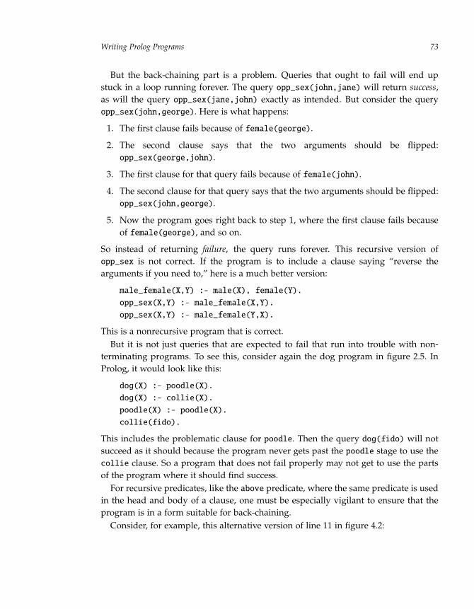
‘‘run’’ --- 2011/9/8 --- 18:05 --- page 73 --- #96�

�

�

�

�

�

�

�


But the back-chaining part is a problem. Queries that ought to fail will end upstuck in a loop running forever. The query opp_sex(john,jane) will return success,as will the query opp_sex(jane,john) exactly as intended. But consider the queryopp_sex(john,george). Here is what happens:

1. The first clause fails because of female(george).

2. The second clause says that the two arguments should be flipped:opp_sex(george,john).

3. The first clause for that query fails because of female(john).

4. The second clause for that query says that the two arguments should be flipped:opp_sex(john,george).

5. Now the program goes right back to step 1, where the first clause fails becauseof female(george), and so on.

So instead of returning failure, the query runs forever. This recursive version ofopp_sex is not correct. If the program is to include a clause saying “reverse thearguments if you need to,” here is a much better version:

male_female(X,Y) :- male(X), female(Y).

opp_sex(X,Y) :- male_female(X,Y).

opp_sex(X,Y) :- male_female(Y,X).

This is a nonrecursive program that is correct.But it is not just queries that are expected to fail that run into trouble with non-

terminating programs. To see this, consider again the dog program in figure 2.5. InProlog, it would look like this:

dog(X) :- poodle(X).

dog(X) :- collie(X).

poodle(X) :- poodle(X).

collie(fido).

This includes the problematic clause for poodle. Then the query dog(fido) will notsucceed as it should because the program never gets past the poodle stage to use thecollie clause. So a program that does not fail properly may not get to use the partsof the program where it should find success.

For recursive predicates, like the above predicate, where the same predicate is usedin the head and body of a clause, one must be especially vigilant to ensure that theprogram is in a form suitable for back-chaining.

Consider, for example, this alternative version of line 11 in figure 4.2:

“run” — 2011/9/8 — 18:05 — page 74 — #97�

�

�

�

�

�

�

�

Chapter 474

above(X,Y) :- above(Z,Y), on(X,Z).

This clause says exactly the same thing as the one in the program; it simply changesthe order of the conjunction. So from the point of view of truth, it works just as wellas the earlier one. It is logically correct. But it does not work well for back-chaining.Consider the query above(b1,b1):

1. The first clause fails because nothing is on block B1.

2. The second clause says to first find a block Z1 such that above(Z1,b1) holds(here renaming the Z variable to Z1).

3. The first clause for above(Z1,b1) fails because nothing is on block B1.

4. The second clause for above(Z1,b1) says to first find a block Z2 such thatabove(Z2,b1) holds (again renaming the Z variable).

5. The program goes back to step 3, where the first clause fails, and so on.

In terms of conjunctive queries to be established, here is how back-chaining wouldwork with this query:

above(b1,b1).

above(Z1,b1), on(b1,Z1).

above(Z2,b1), on(Z1,Z2), on(b1,Z1).

above(Z3,b1), on(Z2,Z3), on(Z1,Z2), on(b1,Z1).

...

It is clear that the conjunctive queries will get longer and longer, and so Prolog willeventually produce an error when it runs out of memory.

When writing recursive programs, there is no simple way to guarantee that theywill terminate. However, a good rule of thumb is that when a clause is recursive, therecursive predicate should appear toward the end of the clause, so that new variablescan be instantiated. Instead of

above(X,Y) :- above(Z,Y), on(X,Z).

write


The two sentences mean the same thing. They are both logically correct. But becauseof the way back-chaining works, the second one will try the recursive predicate onlyafter it has found a value for the variable Z using the on predicate.

When the body of a clause contains a recursive predicate, make sure that its newvariables are instantiated by earlier atoms in the body.

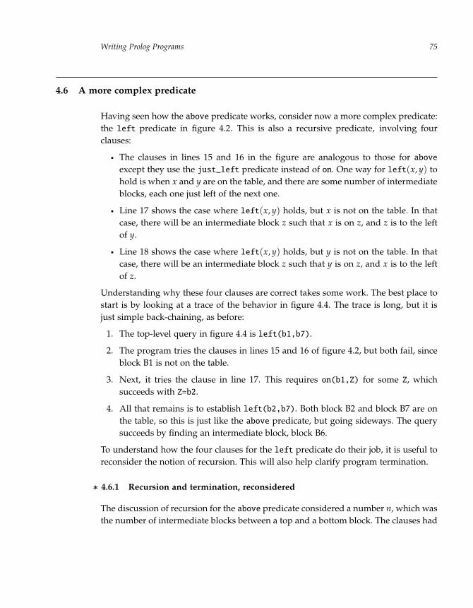
“run” — 2011/9/8 — 18:05 — page 75 — #98�

�

�

�

�

�

�

�


4.6 A more complex predicate

Having seen how the above predicate works, consider now a more complex predicate:the left predicate in figure 4.2. This is also a recursive predicate, involving fourclauses:

The clauses in lines 15 and 16 in the figure are analogous to those for aboveexcept they use the just_left predicate instead of on. One way for left(x, y) tohold is when x and y are on the table, and there are some number of intermediateblocks, each one just left of the next one.

Line 17 shows the case where left(x, y) holds, but x is not on the table. In thatcase, there will be an intermediate block z such that x is on z, and z is to the leftof y.

Line 18 shows the case where left(x, y) holds, but y is not on the table. In thatcase, there will be an intermediate block z such that y is on z, and x is to the leftof z.

Understanding why these four clauses are correct takes some work. The best place tostart is by looking at a trace of the behavior in figure 4.4. The trace is long, but it isjust simple back-chaining, as before:

1. The top-level query in figure 4.4 is left(b1,b7).

2. The program tries the clauses in lines 15 and 16 of figure 4.2, but both fail, sinceblock B1 is not on the table.

3. Next, it tries the clause in line 17. This requires on(b1,Z) for some Z, whichsucceeds with Z=b2.

4. All that remains is to establish left(b2,b7). Both block B2 and block B7 are onthe table, so this is just like the above predicate, but going sideways. The querysucceeds by finding an intermediate block, block B6.

To understand how the four clauses for the left predicate do their job, it is useful toreconsider the notion of recursion. This will also help clarify program termination.

∗ 4.6.1 Recursion and termination, reconsidered

The discussion of recursion for the above predicate considered a number n, which wasthe number of intermediate blocks between a top and a bottom block. The clauses had

“run” — 2011/9/8 — 18:05 — page 76 — #99�

�

�

�

�

�

�

�

Chapter 476

Figure 4.4. Tracing the left predicate

?- left(b1,b7).

Call: (7) left(b1, b7) % This is the main goal.

Call: (8) just_left(b1, b7) % - Try just_left(b1,b7).

Fail: (8) just_left(b1, b7) % This fails.

Redo: (7) left(b1, b7) % Reconsider.

Call: (8) just_left(b1, _L205) % - Try just_left(b1,Z).

Fail: (8) just_left(b1, _L205) % This also fails.


Call: (8) on(b1, _L205) % - Try on(b1,Z) (line 17).

Exit: (8) on(b1, b2) % This succeeds for Z=b2.

Call: (8) left(b2, b7) % - Try left(Z,b7) for Z=b2.

Call: (9) just_left(b2, b7) % - Try just_left(b2,b7).

Fail: (9) just_left(b2, b7) % This fails.


Call: (9) just_left(b2, _L223) % - Try just_left(b2,Z1).

Exit: (9) just_left(b2, b6) % Ok for Z1=b6.

Call: (9) left(b6, b7) % - Try left(b6,b7).

Call: (10) just_left(b6, b7) % - just_left(b6,b7).

Exit: (10) just_left(b6, b7) % This succeeds.

Exit: (9) left(b6, b7) % This succeeds.

Exit: (8) left(b2, b7) % This succeeds.

Exit: (7) left(b1, b7) % The main goal succeeds.

Yes

to work for any n. The key idea was that there was a measure of some sort of the sizeof the queries; a program had to work for queries of any size. In the case of the abovepredicate, the size was the number of intermediate blocks between a top block and abottom block.

Different recursive predicates require different measures of size. Any measure canbe considered but it takes practice to find one that works. In the case of the leftpredicate, the size of a query left(x, y) is the following:

The number of blocks between x and the table +

the number of blocks between y and the table +

the number of blocks on the table between the base of x and the base of y(where the base means the block on the table below it).

So, for example, the size of left(b6,b7) will be 0, the size of left(b1,b7) will be 3,and the size of left(b1,b4) will be 4.

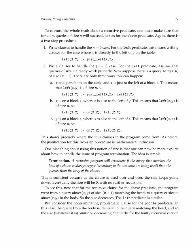
“run” — 2011/9/8 — 18:05 — page 77 — #100�

�

�

�

�

�

�

�


To capture the whole truth about a recursive predicate, one must make sure thatfor all n, queries of size n will succeed, just as for the above predicate. Again, there isa two-step procedure:

1. Write clauses to handle the n = 0 case. For the left predicate, this means writingclauses for the case where x is directly to the left of y on the table:

left(X,Y) :- just_left(X,Y).

2. Write clauses to handle the (n + 1) case. For the left predicate, assume thatqueries of size n already work properly. Now suppose there is a query left(x, y)of size (n + 1). There are only three ways this can happen:

a. x and y are both on the table, and x is just to the left of a block z. This meansthat left(z, y) is of size n, so

left(X,Y) :- just_left(X,Z), left(Z,Y).

b. x is on a block z, where z is also to the left of y. This means that left(z, y) isof size n, so

left(X,Y) :- on(X,Z), left(Z,Y).

c. y is on a block z, where x is also to the left of z. This means that left(x, z) isof size n, so

left(X,Y) :- on(Y,Z), left(X,Z).

This shows precisely where the four clauses in the program come from. As before,the justification for this two-step procedure is mathematical induction.

One nice thing about using this notion of size is that one can now be more explicitabout how to handle the issue of program termination. The idea is simple:

Termination. A recursive program will terminate if the query that matches thehead of a clause is always bigger (according to the size measure being used) than thequeries from the body of the clause.

This is sufficient because as the clause is used over and over, the size keeps goingdown. Eventually the size will be 0, with no further recursion.

To see this, note that for the recursive clause for the above predicate, the programwent from a query above(x, y) of size (n + 1) matching the head, to a query of size n,above(z, y) in the body. So the size decreases. The left predicate is similar.

But consider the nonterminating problematic clause for the poodle predicate. Inthis case, the query from the body is identical to the query matching the head, and sothe size (whatever it is) cannot be decreasing. Similarly, for the faulty recursive version

“run” — 2011/9/8 — 18:05 — page 78 — #101�

�

�

�

�

�

�

�

Chapter 478

Figure 4.5. The start of a trace of a left query

?- left(b3,b3).

Call: (7) left(b3, b3) % The main goal

Call: (8) just_left(b3, b3)

Fail: (8) just_left(b3, b3)


Call: (8) just_left(b3, _L205)

Fail: (8) just_left(b3, _L205)


Call: (8) on(b3, _L205) % Try on(b3,Z).

Exit: (8) on(b3, b4)

Call: (8) left(b4, b3) % Then start left(b4,b3).

Call: (9) just_left(b4, b3)

Fail: (9) just_left(b4, b3)

Redo: (8) left(b4, b3) % Reconsider. ...

of opp_sex, the query from the body is the same as the query matching the head butwith the arguments reversed, and so again the size does not decrease.

Finally, consider the incorrect version of the above predicate (where the order of thetwo conjuncts is changed). It has above(x, y) in the head and above(z, y) in the body,just like the correct version. The difference is that the correct version makes sure thatthe z is lower than x using the on predicate. This guarantees that above(z, y) will besmaller than above(x, y). There is no such guarantee in the incorrect version, so theprogram may not terminate.

4.7 Efficiency in Prolog

So far, the blocks-world program is grammatically correct, logically correct, and inthe right form for back-chaining. It does exactly what is intended. Yet, while it givescorrect results, it does not do so efficiently.

Consider, for example, a trace of the query left(b3,b3). The start is shown infigure 4.5. As the trace continues, the query will eventually fail, as it should. But theeventually is very far away: a full trace would go on for more than 1500 lines. Thereason for this has to do with the way the left predicate is defined in the program.A query left(x, y) is handled in three stages:

1. See if x and y are both on the table (using just_left).

2. See if x is on another block z, and try left with that.

“run” — 2011/9/8 — 18:05 — page 79 — #102�

�

�

�

�

�

�

�


3. See if y is on another block z, and try left with that.

The problem is that this scheme forces the program to reconsider the same queriesover and over.

Look at the pairs of blocks that will be considered in steps 2 and 3:

For left(b3,b3), consider left(b4,b3) and left(b3,b4).



So to establish the query left(b3,b3), the query left(b4,b4) is considered twice(once for left(b4,b3) and once for left(b3,b4)). And, by the same argument, thequery left(b4,b4) requires that left(b5,b5) be considered twice, and left(b5,b5)requires that left(b6,b6) be considered twice. So in trying to answer left(b3,b3),the program will try to establish the query left(b6,b6) a total of 8 (= 2 × 2 × 2)times. If the stack had k blocks in it, the program would try to establish the samebottom query over and over 2k times.

Why should this matter? There are two reasons:

Although modern electronic computers can easily deal with stacks of size k,where k = 20 and even k = 30, no computer can deal with k = 100. The number2100 is so incredibly large that the query would not be answered in our lifetimes.Although the program is guaranteed to terminate eventually, in practical terms itruns forever.

Moreover, such prodigious work is unnecessary. All this effort by Prolog iswasted: back-chaining just ends up failing over and over on exactly the samequeries.

So in the end, Prolog has not been given very good instructions about how to answerthese queries, even though it will produce the right answers.

What can be done? Unfortunately, there is no easy way to write Prolog programsand be sure that they will not do more work than necessary. A good part of computerscience involves analyzing computational problems and coming up with efficientways of solving them. By efficiency is meant “with as little wasted effort as possi-ble.” Among other things, this involves comparing different methods of solving aproblem (called algorithms) and trying to determine which ones will scale the best asthe problem gets bigger.

But each problem needs to be analyzed on its own terms. One needs to think howto structure a Prolog program so that back-chaining can do its job efficiently.

“run” — 2011/9/8 — 18:05 — page 80 — #103�

�

�

�

�

�

�

�

Chapter 480

Figure 4.6. A better procedure for the left predicate left.pl

% A new version of the left(X,Y) predicate.

% The rest of the program (for on, just_left, etc.) is elsewhere.

left(X,Y) :- base(X1,X), base(Y1,Y), table_left(X1,Y1).

% base(Z,X) holds if Z is on the table, below or equal to X.

base(X,X) :- \+ on(X,Y). % X is not on anything.

base(Z,X) :- on(X,Y), base(Z,Y). % X is on a block Y.

% table_left(X,Y): X and Y are on the table, X to the left of Y.

table_left(X,Y) :- just_left(X,Y).

table_left(X,Y) :- just_left(X,Z), table_left(Z,Y).

This book does not spend much time worrying about the efficiency of differentways of solving a problem. But it is worth remembering that not all procedures thatreturn the same answers to the same queries behave in the same way. The followingsection suggests a better algorithm for the left predicate.

∗ A better algorithm

One of the reasons the clauses for left(x, y) are not ideal is that the cases handledby the three clauses are not disjoint. When there is a query left(x, y) that should failwhen neither block x nor block y is on the table, the program looks at the block belowx, generates the left query for that, and after failing, looks at the block below y, andgenerates the left query for that. So both the third and fourth clauses are used. Oneshould always be concerned about efficiency whenever there is a query of size (n + 1)that can generate two recursive queries of size n: there will be two queries of size n,four queries of size (n − 1), eight queries of size (n − 2), and so on. This can lead toan exponential growth in the number of queries.

This exponential behavior can be avoided easily enough. Given a query left(x, y),go directly below x until reaching the table, go directly below y until reaching thetable, and then check the left relationship for just these two base blocks.

This leads to the clauses redefining left in figure 4.6. The predicate base(z, x)holds if z is on the table and is either below x or is x itself. Also, table_left(x, y)holds if x and y are both on the table, with x to the left of y. (The clauses for on andjust_left are not included.)

This version returns the same answers as before, but is a much better algorithm.There would be no problem dealing with thousands and maybe even millions ofblocks. This shows the difference a change in algorithm can make.

“run” — 2011/9/8 — 18:05 — page 81 — #104�

�

�

�

�

�

�

�


Want to read more?

This chapter explained how to write computer programs in Prolog, that is, how torepresent knowledge in a form that can be used effectively by back-chaining. Thisskill is applied throughout the rest of the book.

This chapter is as close as this book gets to traditional computer science. BecauseProlog is a somewhat unusual programming language, it is almost never taught as afirst language in computer science courses. While there is an excellent introductoryprogramming text that uses Prolog [21], most computer science departments startwith languages like Java, Python, or Scheme, for which there are many introductorytextbooks. The sort of programming studied here is called logic programming, which isoften taken up as an advanced topic, using textbooks such as [18, 19, 20, 22].

Computer science goes well beyond programming, however, and one of the topicsstudied in detail is the notion of scalability. How can one manage extremely large com-puter programs without getting lost in the details? Some of the very large computerprograms (such as the program for Microsoft Word, for instance) are among the mostcomplex artifacts ever built by people. How can a team of programmers work on aproject of this size without stepping on each other’s toes?

In another dimension of scale, it is not just programs that become large; the inputsto the program can also be gigantic. For example, there might be a program that ana-lyzes an enormous geographic database or a genome sequence from biology. A majorconcern in computer science is efficiency. How can one write computer programs thatdeal with large inputs like these without taking too long or using too much computermemory?

The approach to programming in this chapter was quite informal. Computer sci-entists learn how to prove mathematically that their programs have certain desirableproperties, for example, that a certain algorithm will eventually produce an expectedresult or that it is as good a way as any to calculate a desired result. Mathematicalinduction often plays a role in this. One of the main topics of theoretical computerscience is the analysis of computational tasks themselves, dividing them into tractableones (for which algorithms exist that will scale well as the input grows) and intractableones (for which there are no good algorithms). As noted at the end of chapter 1,there are tasks that are not even computable, for which there is no algorithm that isguaranteed to terminate at all.

“run” — 2011/9/8 — 18:05 — page 82 — #105�

�

�

�

�

�

�

�

Chapter 482

Exercises

These exercises will give you practice writing and running Prolog programs that rea-son in a simple way about family relationships, mostly exotic flavors of cousins. Beginyour Prolog program by writing a collection of clauses for the child, male, and femalepredicates for some real or imaginary family. To make things interesting, make surethat more than four generations of people are represented. Note that nobody shouldhave more than two parents (one male and one female), but some individuals willhave fewer than two parents recorded. As you work on the following predicates, youshould augment your family as necessary so that each of the predicates you definehas at least one example in your family.

Figure 3.1 showed clauses for the predicates parent, father, and grand_father.Now write clauses for each of the following predicates (and for any other auxiliarypredicates you find useful):

1. mother, grand_parent, and great_grand_mother.

2. sibling, brother, and sister.x is a sibling of y if x and y are two different people who share a parent incommon. A brother is a sibling who is male; a sister is a sibling who is female.

3. half_sibling and full_sibling.Half siblings are siblings who have exactly one parent in common. Full siblingsare siblings who have two parents in common.

4. first_cousin and second_cousin.x is a first cousin of y if some parent of x and some parent of y are siblings. (Notethat first cousins will have a grandparent in common.) x and y are second cousinsif some parent of x and some parent of y are first cousins. (Second cousins willshare a great-grandparent.)

5. half_first_cousin and double_first_cousin.x is a half first cousin of y if some parent of x is a half sibling of a parent of y. xis a double first cousin of y if each parent of x is a sibling of a parent of y. (Notethat a first cousin is not the same thing as a double half first cousin. The doubleand half do not cancel out.)

6. first_cousin_twice_removed.Look on the Internet or elsewhere for the definition of a third cousin once

“run” — 2011/9/8 — 18:05 — page 83 — #106�

�

�

�

�

�

�

�


removed or a second cousin twice removed and so on, and fill in the detailshere.

7. descendant, ancestor.x is a descendant of y if x is either a child of y or (recursively) of someone whois a descendant of y. x is an ancestor of y if y is a descendant of x.

8. cousin.x is a cousin of y if some parent of x and some parent of y are either siblingsor (recursively) cousins. (The x and y will always end up being nth cousins forsome n. For example, fourth cousins will have parents who are third cousins.)

9. closest_common_ancestor.x is a closest common ancestor of two people y and z if x is an ancestor of bothy and z and no child of x is an ancestor of y and z. (A closest common ancestorof two first cousins will be someone who is a grandparent of both.)

10. write_descendant_chain.Later chapters examine the special predicates write and nl, which can be usedto produce output other than just the values of variables. For example, if there isa clause

write_child(X,Y) :-

write(X), write(’ is a child of ’), write(Y), nl.

then the query write_child(john_smith,sue_jones) will always succeed andwill also print

john_smith is a child of sue_jones

on one line. Include this predicate in your program, and write the clausesfor a predicate write_descendant_chain(x, y) that prints a chain from x toy when x is a descendant of y but prints nothing when x is not a descen-dant of y. For example, if John Smith is a descendant of William Brown,then write_descendant_chain(john_smith,william_brown) should print asequence of lines something like this:

john_smith is a child of sue_jones

sue_jones is a child of harvey_jones

harvey_jones is a child of davy_jones

davy_jones is a child of anna_brown

anna_brown is a child of william_brown

“run” — 2011/9/8 — 18:05 — page 84 — #107�

�

�

�

�

�

�

�

Chapter 484

Hint: You will not be able to use the descendant predicate you defined for this.Use the child predicate together with write_child. Also, work down from yrather than up from x.

In case you were wondering, these questions do not exhaust the varieties of cousinspeople have considered. Anthropologists distinguish between parallel and cross firstcousins, according to whether or not the two parents who are siblings are of the samesex. And once the idea of people being married is included, there are new possibilities:step-siblings (children of the spouse of a parent who are not siblings) and siblings-in-law in two varieties (a sibling of a spouse and the spouse of a sibling). This lead tostep first cousins and two varieties of first cousins-in-law. And so on.

“run” — 2011/9/8 — 18:05 — page 85 — #108�

�

�

�

�

�

�

�

5 Case Study: Satisfying Constraints

This chapter returns to the central conjecture of the book, namely, that ordinarythinking can be viewed as a form of computation.

One of the difficulties in observing and analyzing our own thinking is that somuch of it happens so quickly that it is hard to describe exactly what takes place. Anexample is resolving the pronoun it in the trophy-suitcase sentences in chapter 1. Butnot all thinking is like this, fortunately. Consider working on a puzzle that appearsin a newspaper. There, the reasoning can go on for minutes, even hours. This isthe sort of thinking that is the subject matter of this chapter. The thinking neededto solve a wide variety of reasoning puzzles can be formulated in the same way, interms of constraint satisfaction problems. This chapter describes five different constraintsatisfaction problems. (Chapter 6 shows that some parts of visual interpretation canalso be formulated in this way.)

The approach to constraint satisfaction problems here is not that of an expert butmore of a novice, with considerable trial-and-error and guesswork involved. The Pro-log programs presented in this chapter work well enough for the easiest forms ofthe puzzles but will gradually stop working as the puzzles get harder. (What makesa puzzle hard is one of the issues to be discussed.) Some time is spent trying todo better than guessing, but this is not the main focus. Finding ways to cope withchallenging puzzles as an expert would is a whole area of research in itself (calledconstraint programming) that is beyond the scope of this book.

In working through various examples of constraint satisfaction problems, new fea-tures of Prolog are introduced as needed, for example, producing output (to displayhelpful messages), anonymous variables (to avoid having to give names to variables),and numbers (to do arithmetic in Prolog).

The first section of this chapter introduces the idea of constraint satisfaction prob-lems and presents a general way of solving them. Each of the five remaining sectionstakes on a different constraint satisfaction problem (Sudoku, cryptarithmetic, the

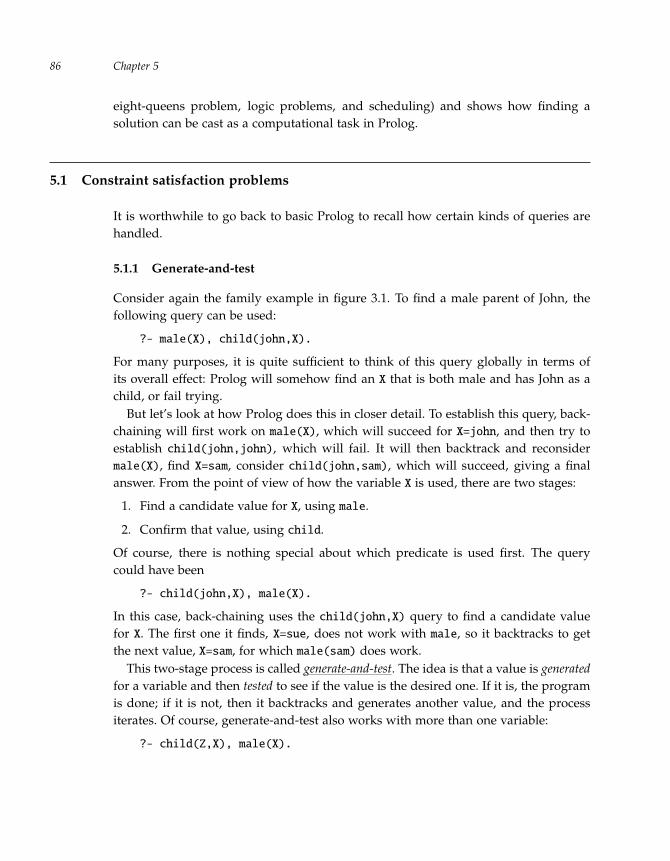
“run” — 2011/9/8 — 18:05 — page 86 — #109�

�

�

�

�

�

�

�

Chapter 586

eight-queens problem, logic problems, and scheduling) and shows how finding asolution can be cast as a computational task in Prolog.

5.1 Constraint satisfaction problems

It is worthwhile to go back to basic Prolog to recall how certain kinds of queries arehandled.

5.1.1 Generate-and-test

Consider again the family example in figure 3.1. To find a male parent of John, thefollowing query can be used:

?- male(X), child(john,X).

For many purposes, it is quite sufficient to think of this query globally in terms ofits overall effect: Prolog will somehow find an X that is both male and has John as achild, or fail trying.

But let’s look at how Prolog does this in closer detail. To establish this query, back-chaining will first work on male(X), which will succeed for X=john, and then try toestablish child(john,john), which will fail. It will then backtrack and reconsidermale(X), find X=sam, consider child(john,sam), which will succeed, giving a finalanswer. From the point of view of how the variable X is used, there are two stages:

1. Find a candidate value for X, using male.

2. Confirm that value, using child.

Of course, there is nothing special about which predicate is used first. The querycould have been

?- child(john,X), male(X).

In this case, back-chaining uses the child(john,X) query to find a candidate valuefor X. The first one it finds, X=sue, does not work with male, so it backtracks to getthe next value, X=sam, for which male(sam) does work.

This two-stage process is called generate-and-test. The idea is that a value is generatedfor a variable and then tested to see if the value is the desired one. If it is, the programis done; if it is not, then it backtracks and generates another value, and the processiterates. Of course, generate-and-test also works with more than one variable:

?- child(Z,X), male(X).

‘‘run’’ --- 2011/9/8 --- 18:05 --- page 87 --- #110�

�

�

�

�

�

�

�

Case Study: Satisfying Constraints 87

In this case, candidate pairs of values are considered. The first pair generated is Z=johnand X=sue. But the test male(sue) fails, and so the program backtracks and generatesthe next pair of values, which is Z=john and X=sam, and which passes the test.

Now consider the following query:

?- male(X), child(Z,X), child(jane,Z).

Tracing the back-chaining, one can see that generate-and-test is used repeatedly:

1. Using male(X), generate a first value for X, and get X=john.

a. Generate a Z for this X using child(Z,X), which fails.

2. Backtrack and generate a second value for X, which is X=sam.

a. Generate a Z for this X using child(Z,X), and get Z=john.

This fails the test child(jane,Z).

b. Backtrack and generate the next Z, which is Z=jane.

This fails the test child(jane,Z).

c. Backtrack for yet another Z. However, there are no other values for Z, and sothe program is unable to generate a Z for this X.

3. Backtrack and generate a third value for X using male(X), which is X=george.

a. Generate a Z for this X using child(Z,X), and get Z=sue.

This passes the test child(jane,Z), and so the program is done.

This generate-and-test process, which back-chaining does automatically, is at the rootof how constraint satisfaction problems can be solved.

A simple example: Map coloring

Look at the map-coloring problem in figure 5.1. We seek a Prolog program that solvesthis problem and finds colors for the five countries. A program that does so appearsin figure 5.2. This program can be understood by reading the clause for the solutionpredicate in English:

If a, b, c, d, and e are colors, and if

a �= b, a �= c, a �= d, a �= e, b �= c, c �= d, and d �= e,

then these colors are a solution to the given map-coloring problem.

Since the only colors are the three given ones, red, white, and blue, the solutionpredicate produces correct answers:

“run” — 2011/9/8 — 18:05 — page 88 — #111�

�

�

�

�

�

�

�

Chapter 588

Figure 5.1. A map-coloring problem

A map is depicted here with countries named A, B, C,D, and E. The goal is to color the countries on the mapusing just the colors red, white, and blue in such a waythat no two countries with a border between them havethe same color.

Figure 5.2. Coloring the map of figure 5.1 map.pl

% solution(A,B,C,D,E) holds if A,B,C,D,E are colors

% that solve a map-coloring problem from the text.

solution(A,B,C,D,E) :-

color(A), color(B), color(C), color(D), color(E),

\+ A=B, \+ A=C, \+ A=D, \+ A=E, \+ B=C, \+ C=D, \+ D=E.

% The three colors are these.

color(red).

color(white).

color(blue).

?- solution(A,B,C,D,E).

A = red, B = white, C = blue, D = white, E = blue

(Note: From now on, some figures omit the Yes answer to a query and display thevalues of variables on a single line.)

This program works by generate-and-test, generating values for the variables A, B,C, D, and E using the color predicate, and then testing whether the values satisfy therequired inequalities. If they do, the program is done; otherwise it backtracks andgenerates new values. (There is more than one correct solution to this problem.)

Note that tracing the behavior of this program would show that Prolog does quite abit of work before it actually finds a solution. Roughly speaking, this is because all thegenerating is done before any testing. This issue is discussed in detail in section 5.3.3.

“run” — 2011/9/8 — 18:05 — page 89 — #112�

�

�

�

�

�

�

�


5.1.2 Variables, domains, constraints

Map coloring is a very simple example of a constraint satisfaction problem. In general,these are made up of the following three components:

There are some number of variables for which values are to be found. In thecase of map coloring, the variables A, B, C, D, E represent the colors of the fivecountries.

Each variable gets a value from some finite domain of values. In the case of mapcoloring, each variable has the same domain: the colors red, white, and blue.

There are constraints to be satisfied among subsets of the variables. In the caseof map coloring, the constraints are that the colors of countries with bordersbetween them must be different.

A solution to a constraint satisfaction problem is an assignment of a value to eachvariable (taken from the domain of the variable) such that all the constraints aresatisfied. In other words, solving a constraint satisfaction problem means findingvalues for the variables subject to the constraints.

The simplest way to solve a constraint satisfaction problem in Prolog is to usegenerate-and-test: generate values from the domain for each variable, and then test tosee if all the constraints are satisfied, backtracking as necessary.

A Prolog program that solves an arbitrary constraint satisfaction problem usinggenerate-and-test can be constructed using a format somewhat like the following:

solution(Variable1,Variable2,. . .,Variablen) :-

domain1(Variable1),. . .

domainn(Variablen),

constraint1(Variable, . . . , Variable),. . .

constraintm(Variable, . . . , Variable).

This is the form used for the map coloring.

5.1.3 Output in Prolog

When a Prolog query succeeds, it displays values for all the variables. To make theanswer easier to read, however, it is often useful to display more. Prolog provides twospecial predicates that can be used for this in queries or in the bodies of clauses:

“run” — 2011/9/8 — 18:05 — page 90 — #113�

�

�

�

�

�

�

�

Chapter 590

The predicate write(term) is considered to always succeed, and it has the effectof printing the value of the term.

The predicate nl (for newline) with no arguments is considered to alwayssucceed, and it has the effect of going to a new line of output.

To see how these work, look at how the following queries are answered:

?- X=joe, write(’variable X is ’), write(X), write(’!!’).

variable X is joe!!

X = joe

Yes

?- write(’Paris in the’), nl, write(’ spring.’).

Paris in the

spring.

Yes

So with these predicates, the solution to the map-coloring problem can be displayedbetter by adding the following clause to the program of figure 5.2:

print_colors :-

solution(A,B,C,D,E), nl,

write(’Country A is colored ’), write(A), nl,

write(’Country B is colored ’), write(B), nl,

write(’Country C is colored ’), write(C), nl,

write(’Country D is colored ’), write(D), nl,

write(’Country E is colored ’), write(E), nl.

The predicate print_colors first finds a solution to the constraint satisfactionproblem using solution, and then prints it in a readable form:

?- print_colors.

Country A is colored red

Country B is colored white

Country C is colored blue

Country D is colored white

Country E is colored blue

Note that the query in this case no longer has variables. All the variables are withinthe clause for the print_colors predicate and are displayed explicitly using writeand nl. This does not change the thinking involved in producing a solution. But itresults in a much more convenient program, since anyone running the program doesnot have to know in advance how to use or interpret the variables.

“run” — 2011/9/8 — 18:05 — page 91 — #114�

�

�

�

�

�

�

�


Figure 5.3. A 4 × 4 Sudoku problem

NW NE

SESW

You are given a 4 × 4 grid, where some of the cells are blank andsome contain numbers between 1 and 4. Fill in all the blank cellswith numbers between 1 and 4 so that

the numbers in each row (1, 2, 3, 4) are unique,

the numbers in each column (1, 2, 3, 4) are unique,

the numbers in each 2 × 2 quadrant (NW, NE, SW, SE) areunique.

5.2 A first example: Sudoku

Figure 5.3 shows a 4 × 4 Sudoku problem. It is a simpler version of Sudoku than the9 × 9 version that appears in newspapers and puzzle books. (Section 5.2.3 discussesthe 9 × 9 version.)

5.2.1 The anonymous variable in Prolog

A certain feature of Prolog, the anonymous variable, is useful for solving the Sudokuproblem. Prolog allows the underscore character _ to be used as a variable in thosecases where the goal is not finding the value of the variable but ensuring that there isone:

?- child(X,sue). % Who is a child of Sue?

X=john

Yes

?- child(_,sue). % Does Sue have a child?

Yes

?- child(_,john). % Does John have a child?

No

?- child(_,_). % Does anyone have a child?

Yes

Note that each occurrence of the anonymous variable can be for a different value. Sothe last query behaves like child(X,Y), rather than like child(X,X).

“run” — 2011/9/8 — 18:05 — page 92 — #115�

�

�

�

�

�

�

�

Chapter 592

Figure 5.4. Using the sudoku predicate

?- sudoku( % Note the anonymous variables in the query.

1, 4, _, _,

_, _, 4, _,

2, _, _, _,

_, _, _, 3

).

A solution to this puzzle is

1 4 3 2

3 2 4 1

2 3 1 4

4 1 2 3

This anonymous variable can be used to explain what a Sudoku program shoulddo. The user provides a partial solution to the problem and asks the program to printa complete solution. A query is posed with some of the entries filled in the grid, andthe program will print all sixteen entries in a tabular format (see figure 5.4). The top-level predicate is sudoku. Note that the solution shown in the figure satisfies all theconstraints: each row, column, and quadrant uses the numbers 1, 2, 3, and 4.

5.2.2 Sudoku as constraint satisfaction

It is easy to see Sudoku as a constraint satisfaction problem:

There are sixteen variables, one for each entry in the grid.

The domain for each variable is {1, 2, 3, 4}.

The constraints to be satisfied are the following: for each row, column, andquadrant, the four variables must have distinct values.

Assuming there is a solution predicate that takes sixteen arguments and solves theconstraint satisfaction problem, it is not hard to define the top-level sudoku predicatethat does the printing (see the top half of figure 5.5, above the dashed line). Thesudoku predicate uses solution to find a solution, then prints a one-line message,and finally uses the predicate printrow four times to print out each of the rows. Aswith print_colors, all the thinking happens in the solution predicate.

Let us now turn to this solution predicate. The easiest way to write the predicateis to first define a predicate uniq that takes four arguments and ensures that they areall different from each other:

uniq(P,Q,R,S) :- \+ P=Q, \+ P=R, \+ P=S, \+ Q=R, \+ Q=S, \+ R=S.

“run” — 2011/9/8 — 18:05 — page 93 — #116�

�

�

�

�

�

�

�


Figure 5.5. A Sudoku solver sudoku.pl

% The main predicate. Solve the puzzle and print the answer.

% The variable Rij stands for the number in row i and column j.

sudoku(R11,R12,R13,R14,R21,R22,R23,R24,R31,R32,R33,R34,

R41,R42,R43,R44) :-

solution(R11,R12,R13,R14,R21,R22,R23,R24,R31,R32,R33,R34,

R41,R42,R43,R44),

nl, write(’A solution to this puzzle is’), nl,

printrow(R11,R12,R13,R14), printrow(R21,R22,R23,R24),

printrow(R31,R32,R33,R34), printrow(R41,R42,R43,R44).

% Print a row of four numbers with spaces between them.

printrow(P,Q,R,S) :- write(’ ’), write(P), write(’ ’), write(Q),

write(’ ’), write(R), write(’ ’), write(S), nl.

%------------------------------------------------------------------

solution(R11,R12,R13,R14,R21,R22,R23,R24,R31,R32,R33,R34,

R41,R42,R43,R44) :-

uniq(R11,R12,R13,R14), uniq(R21,R22,R23,R24), % rows 1,2

uniq(R31,R32,R33,R34), uniq(R41,R42,R43,R44), % rows 3,4

uniq(R11,R21,R31,R41), uniq(R12,R22,R32,R42), % cols 1,2

uniq(R13,R23,R33,R43), uniq(R14,R24,R34,R44), % cols 3,4

uniq(R11,R12,R21,R22), uniq(R13,R14,R23,R24), % NW and NE

uniq(R31,R32,R41,R42), uniq(R33,R34,R43,R44). % SW and SE

% uniq holds if P,Q,R,S are all distinct nums (from 1 to 4).

uniq(P,Q,R,S) :- num(P), num(Q), num(R), num(S),

\+ P=Q, \+ P=R, \+ P=S, \+ Q=R, \+ Q=S, \+ R=S.

% The four numbers to go into each cell

num(1). num(2). num(3). num(4).

So uniq(1,3,2,4) succeeds, but uniq(1,3,2,3) fails. (This idea of having a certainnumber of values that are different from each other shows up in many constraintsatisfaction problems.)

As written, however, the uniq predicate can only be used to test the four argumentsfor uniqueness, not to generate them. This is because negation needs its arguments tobe instantiated (see section 3.2.3). Assuming there is a predicate num that can test orgenerate the numbers from 1 to 4, the uniq predicate can be rewritten so that it willtest or generate a group of four numbers from 1 to 4 that are unique. Then, usingthis predicate for each row, column, or quadrant, one can test or generate a group ofsixteen numbers that solves the Sudoku problem. This is shown in the bottom half offigure 5.5.

“run” — 2011/9/8 — 18:05 — page 94 — #117�

�

�

�

�

�

�

�

Chapter 594

How does this solution predicate work? It needs to generate sixteen values. Itstarts by using uniq(R11,R12,R13,R14) to generate four distinct values for the vari-ables of row 1. Then it does the same for rows 2, 3, and 4. At this point, all sixteenvariables have values. It then tests uniq(R11,R21,R31,R41), which is for the variablesof column 1. If these four values are distinct, it continues and tests the distinctnessof columns 2, 3, and 4; if they are not distinct, the test fails, and it backtracks togenerate new values for the variables in row 4 or 3 or 2 or perhaps all the way backto row 1, as necessary. Once all the column tests succeed, the solution predicatetests uniq(R11,R12,R21,R22), which is for the variables of the NW quadrant. If thesefour values are distinct, it tests the quadrants NE, SW, and SE in turn; if they are notdistinct, it again backtracks all the way to the rows and tries to generate new values.If all the column and quadrant tests are successful, a solution has been found, andthe program is done.

5.2.3 Search spaces

It is easy to generalize this 4 × 4 solution to 9 × 9 Sudoku puzzles. Instead of havingtwelve constraints (for rows, columns, and quadrants) over sixteen variables, therewould be twenty-seven constraints over eighty-one variables.

Will this work? The answer is, in principle, definitely yes; in practice, definitely no.The problem is that the 9 × 9 Sudoku puzzle is much larger than the 4 × 4 one. Justhow much larger is worth investigating further.

A useful measure of the size of a constraint satisfaction problem is the size of itssearch space. The search space is the collection of all the different ways the variables ofa problem can be assigned values from the domain before taking the constraints intoaccount.

For a 4× 4 Sudoku, each of the sixteen variables can take on four possible values.So there are 4 × 4 × · · · × 4 = 416 possible assignments to the variables, which isabout 4 × 109 (four billion). This is considered to be small (for computers).

For a 9 × 9 Sudoku puzzle, each of the eighty-one variables can take on ninepossible values. So there are 9 × 9 × · · · × 9 = 981 possible assignments to thevariables, which is about 2 × 1077. This is considered to be enormous.

To understand the insurmountable difficulty this second number poses even for thefastest supercomputers, it is useful to do a thought experiment:

1. Imagine that there is a supercomputer capable of exploring a billion variableassignments per second in the search space. (No existing computer is fast enoughto do this.)

“run” — 2011/9/8 — 18:05 — page 95 — #118�

�

�

�

�

�

�

�


2. Imagine that by virtue of new technology received from outer space, this super-computer suddenly becomes one billion times faster. This means that jobs thatused to take it ten years to do can now be done in under one second.

3. Imagine that there are one billion of these supercomputers and that they can allbe made to work together, sharing the job of exploring the search space.

Then,

How many variable assignments can be explored per second?The answer is 109 × 109 × 109 = 1027.

So how long would it take to go through the 9 × 9 Sudoku search space?The answer is 981 ÷ 1027 = 2 × 1050 seconds, or about 6 × 1040 centuries.

Given these sorts of numbers, it should be no surprise that the generate-and-testprogram to solve the 9 × 9 Sudoku problem does not work very well.

5.2.4 Guessed values and forced values

This analysis of the search space seems to be suggest that even the fastest computerswould not be able to solve a 9 × 9 Sudoku problem. But this is not quite right. Theanalysis shows that no computer (or person) would be able to explore the entireSudoku search space because it is too large. But, in fact, computers and people areable to solve Sudoku problems. How they do so is very different from the methodused in the 4 × 4 case.

The problem with the way the Sudoku and map-coloring problems were solvedis that there was far too much guessing: making a random selection from the searchspace and then backtracking if it was not right. Sudoku experts do not think thisway. They do very little guessing, and only for the most difficult puzzles (the onessometimes called devilish). Instead, they repeatedly try to see if the constraints of thepuzzle force the values for certain entries based on the known values of other entries.

For example, figure 5.6 shows a 4 × 4 Sudoku problem with a 3 located at position(1, 1) (top left) and at position (4, 4) (bottom right). It is not hard to see that theremust be a 3 at (2, 3) and another at (3, 2). These two entries are forced.

Programming this type of algorithm for Sudoku would take some work. Thebasic idea of using forced values to minimize the guesswork is explored in the nextconstraint satisfaction problem, cryptarithmetic.

‘‘run’’ --- 2011/9/8 --- 18:05 --- page 96 --- #119�

�

�

�

�

�

�

�

Chapter 596

Figure 5.6. Forced values in Sudoku

3

3

��

��

There is only one possible location for a 3 on thesecond row: it must be located at position (2, 3).The other three locations are ruled out by the 3 atposition (1, 1) and the one at position (4, 4).

The 3 on the third row is similar.

5.3 A second example: Cryptarithmetic

Cryptarithmetic problems are of the following form. Given is an equation using letterslike this:

SEND

+ MORE

MONEY

A distinct digit must be found for each letter such that the equation holds. (Also, theleading leftmost digits, S and M, must not be 0.) A solution for this example is

S = 9, E = 5, N = 6, D = 7, M = 1, O = 0, R = 8, Y = 2

since 9567 + 1085 = 10652. As a preliminary to solving problems like this in Prolog,the next section examines the facilities Prolog provides for arithmetic.

5.3.1 Arithmetic in Prolog

Numbers in Prolog were first mentioned in the review in figure 3.10, which said that aProlog term is either a constant, variable, or number, and that a number is a sequenceof one or more digits optionally preceded by a minus sign and optionally containinga decimal point (for rational numbers).

Since numbers are terms, they can appear in programs and queries anywhere aconstant or variable can appear. So Prolog program can have clauses like

age(donna,23).

age(andy,22).

current_temperature(-5.2).

and queries like the following:

“run” — 2011/9/8 — 18:05 — page 97 — #120�

�

�

�

�

�

�

�


?- age(donna,N).

N = 23

Yes

?- age(X,N), \+ N=23.

X = andy, N = 22

Yes

But what makes numbers especially useful is that Prolog provides arithmetic oper-ations over them. Specifically, going back to figure 3.10, the notion of a literal (thebuilding block of queries and bodies of clauses) can be generalized to include thefollowing arithmetic relations, optionally preceded by the negation sign:

less than: E1 < E2

greater than: E1 > E2

less than or equal: E1 =< E2

greater than or equal: E1 >= E2

equal: E1 =:= E2

equal: Variable is E

The Ei mentioned here are arithmetic expressions, that is, formulas built out of numbersand variables using parentheses and the operations + (addition), - (subtraction), *(multiplication), / (division), ** (exponentiation), and others. So here is an arithmeticexpression in Prolog:

(X-Y)**2 + 3*(X/Y)

Note that this is not a Prolog term, atom, or literal; the grammar is clearly all wrong.Arithmetic expressions like these can only be used within Prolog programs andqueries in very specific contexts. In particular, they can only be used as an E in oneof the arithmetic relations just listed.

Here then are some legal Prolog queries that use arithmetic expressions and theanswers they produce:

?- X=3, (X+4) > 2*X.

X = 3

Yes

?- X=3, (X+2) >= 2*X + 1.

No

‘‘run’’ --- 2011/9/8 --- 18:05 --- page 98 --- #121�

�

�

�

�

�

�

�

Chapter 598

One restriction on the use of arithmetic expressions is that the variables in them mustalready have values:

?- X=4, X > 2.

X = 4

Yes

?- X > 2, X=4.

ERROR: Arguments are not sufficiently instantiated

In requiring variables to be instantiated, arithmetic expressions are like the \+ oper-ation. One exception to this rule is the is operation: the left-hand side must be avariable and it need not have a value; the right-hand side is an arithmetic expression,where all the variables must have values:

?- Y=2, X=5, X is Y+4.

No

?- Y=2, X is Y+4.

X = 6, Y = 2

Yes

Using the is relation is the normal way of getting the value of an arithmeticexpression to use with another predicate. In other words,

q(Y), p(Y+4,Z).

is not a legal query, since Y+4 is not a term (it is an arithmetic expression). But

q(Y), X is Y+4, p(X,Z).

is correct (assuming q is being used to generate a numeric value for Y).

Arithmetic programs

With arithmetic expressions, Prolog programs can perform numeric calculations.Suppose, for example, that a program has the following clauses:

birth_year(donna,1986).

birth_year(andy,1987).

current_year(2012).

Then the following clause calculates the age of a person from the current year:

% Age of a person P is the current year minus the birth year.

age(P,X) :- birth_year(P,Y1), current_year(Y2), X is Y2-Y1.

This gives the following behavior:

“run” — 2011/9/8 — 18:05 — page 99 — #122�

�

�

�

�

�

�

�


Figure 5.7. A program for n! factorial.pl

% factorial(N,M) holds when M=Nx(N-1)x...x2x1.

factorial(1,1).

factorial(N,M) :- N > 1, N1 is N-1, factorial(N1,K), M is N*K.

?- age(andy,N).

N = 25

Yes

Although they are not the focus of this book, one can also write more traditionalnumerical programs in Prolog, for example, a program to compute the value ofn!, defined as n × (n − 1) × (n − 2) × · · · × 2 × 1. What is needed is a predicatefactorial(n, m) that holds when n! = m. This can be written as a recursive pred-icate, observing that for n > 1, the factorial n! = n × (n − 1)!. The entire program forthe factorial is shown in figure 5.7.

5.3.2 Cryptarithmetic as constraint satisfaction

Let us now return to the cryptarithmetic problem. The solution to this problem usesarithmetic expressions that deal with integers, in particular, // (integer quotient) andmod (integer remainder). For instance,

?- X is 11/3, Y is 11//3, Z is 11 mod 3.

X = 3.66667, Y = 3, Z = 2

Whereas / does full division, the // operation produces the integer part of a division,and mod produces the remainder after an integer division. When these two operationsare used with 10, the result is the sum and carry digits of an addition:

?- S is (2+5) mod 10, C is (2+5) // 10,

S = 7, C = 0

Yes

?- S is (8+5) mod 10, C is (8+5) // 10,

S = 3, C = 1

Yes

In the first case, the sum digit for (2 + 5) is 7 with a carry digit of 0 (that is, the sumis 7), and in the second, the sum digit for (8 + 5) is 3 with a carry digit of 1 (that is,the sum is 13).

“run” — 2011/9/8 — 18:05 — page 100 — #123�

�

�

�

�

�

�

�

Chapter 5100

Figure 5.8. SEND+MORE=MONEY v1 sendmore1.pl

% solution(...) holds for a solution to SEND+MORE=MONEY.

solution(S,E,N,D,M,O,R,Y) :-

uniq_digits(S,E,N,D,M,O,R,Y), S > 0, M > 0,

Y is (D+E) mod 10, C1 is (D+E) // 10,

E is (N+R+C1) mod 10, C10 is (N+R+C1) // 10,

N is (E+O+C10) mod 10, C100 is (E+O+C10) // 10,

O is (S+M+C100) mod 10, M is (S+M+C100) // 10.

% uniq(...) holds if the arguments are all distinct digits.

uniq_digits(S,E,N,D,M,O,R,Y) :-

dig(S), dig(E), dig(N), dig(D), dig(M), dig(O), dig(R), dig(Y),

\+ S=E, \+ S=N, \+ S=D, \+ S=M, \+ S=O, \+ S=R, \+ S=Y,

\+ E=N, \+ E=D, \+ E=M, \+ E=O, \+ E=R, \+ E=Y,

\+ N=D, \+ N=M, \+ N=O, \+ N=R, \+ N=Y,

\+ D=M, \+ D=O, \+ D=R, \+ D=Y,

\+ M=O, \+ M=R, \+ M=Y,

\+ O=R, \+ O=Y,

\+ R=Y.

% The digits

dig(0). dig(1). dig(2). dig(3). dig(4).

dig(5). dig(6). dig(7). dig(8). dig(9).

The SEND + MORE = MONEY equation gives a series of equations involving thesum and carry digits. For example, for the units digits, the sum digit for (D + E)must be Y. If the carry digit for this sum is C1, then for the tens digit, the sum digitfor (N + R + C1) must be E. The hundreds and thousands digits will be similar.

It is not hard to see this cryptarithmetic problem as a constraint satisfaction one:

The variables will be the letters that are mentioned in the puzzle, S, E, N, D, M,O, R, Y, as well variables for the carry digits.

The letter variables will take their values from 0 to 9; the carry-digit variableswill be 0 or 1.

The constraints to be satisfied are that the digits are unique; that S > 0, M > 0;and that all the digit equations for the sum and carry digits are satisfied.

A Prolog program that solves this puzzle is shown in figure 5.8. The predicateuniq_digits ensures that all its arguments are distinct digits (using the predicatedig). The solution predicate checks for uniqueness and ensures that the digitequations are satisfied using // and mod. It uses variables for the carry digits, C1,C10, C100, coming from the units, tens, and hundreds columns, respectively.

“run” — 2011/9/8 — 18:05 — page 101 — #124�

�

�

�

�

�

�

�


One can confirm that this program does the right thing:

?- solution(S,E,N,D,M,O,R,Y).

S = 9, E = 5, N = 6, D = 7, M = 1, O = 0, R = 8, Y = 2

There is a problem, however. It takes too long, over ninety seconds even on a fastcomputer. To do better, guesswork must be minimized.

5.3.3 Minimizing the guesswork: Two rules

There are two rules that help minimize guesswork in this and other constraint satis-faction problems. They allow the solution of much more challenging problems withlarge search spaces. Here is the first:

Rule 1. If a value is fully determined by other values, then avoid guessing the valueand later testing if it is correct.

For example, suppose there are two predicates uniq2 and uniq3 that can test orgenerate two or three distinct values, respectively. Then instead of writing this:

uniq3(A,B,C), % Guess at A,B,C.

B is (A+C) mod 10 % Then test if B is ok.

write this:

uniq2(A,C), % Guess at A and C.

B is (A+C) mod 10, % Calculate B once.

uniq3(A,B,C) % Test that all values are unique.

The first version has a search space of 10× 10× 10 = 1000, but the second has a searchspace of only 10 × 10 = 100.

The second rule is this:

Rule 2. Avoid placing independent guesses between the generation and the testingof other values.

Then instead of writing this:

dig(A), dig(B), % Guess at A and B.

dig(C), dig(D), % Guess at C and D.

A > B % Test for A and B.

write this:

dig(A), dig(B), % Guess at A and B.

A > B, % Test for A and B.

dig(C), dig(D) % Guess at C and D.

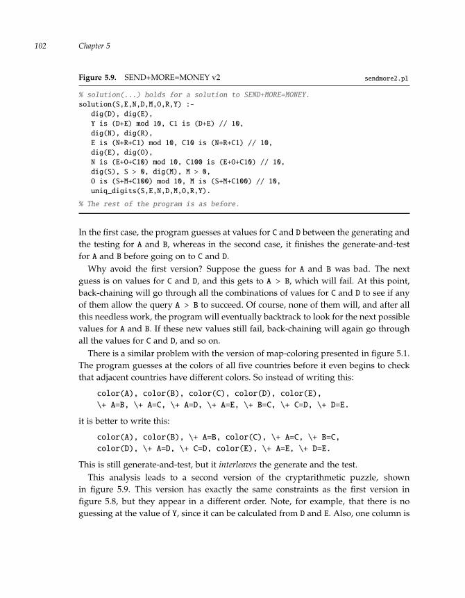
“run” — 2011/9/8 — 18:05 — page 102 — #125�

�

�

�

�

�

�

�

Chapter 5102

Figure 5.9. SEND+MORE=MONEY v2 sendmore2.pl

% solution(...) holds for a solution to SEND+MORE=MONEY.

solution(S,E,N,D,M,O,R,Y) :-

dig(D), dig(E),

Y is (D+E) mod 10, C1 is (D+E) // 10,

dig(N), dig(R),

E is (N+R+C1) mod 10, C10 is (N+R+C1) // 10,

dig(E), dig(O),

N is (E+O+C10) mod 10, C100 is (E+O+C10) // 10,

dig(S), S > 0, dig(M), M > 0,

O is (S+M+C100) mod 10, M is (S+M+C100) // 10,

uniq_digits(S,E,N,D,M,O,R,Y).

% The rest of the program is as before.

In the first case, the program guesses at values for C and D between the generating andthe testing for A and B, whereas in the second case, it finishes the generate-and-testfor A and B before going on to C and D.

Why avoid the first version? Suppose the guess for A and B was bad. The nextguess is on values for C and D, and this gets to A > B, which will fail. At this point,back-chaining will go through all the combinations of values for C and D to see if anyof them allow the query A > B to succeed. Of course, none of them will, and after allthis needless work, the program will eventually backtrack to look for the next possiblevalues for A and B. If these new values still fail, back-chaining will again go throughall the values for C and D, and so on.

There is a similar problem with the version of map-coloring presented in figure 5.1.The program guesses at the colors of all five countries before it even begins to checkthat adjacent countries have different colors. So instead of writing this:

color(A), color(B), color(C), color(D), color(E),

\+ A=B, \+ A=C, \+ A=D, \+ A=E, \+ B=C, \+ C=D, \+ D=E.

it is better to write this:

color(A), color(B), \+ A=B, color(C), \+ A=C, \+ B=C,

color(D), \+ A=D, \+ C=D, color(E), \+ A=E, \+ D=E.

This is still generate-and-test, but it interleaves the generate and the test.This analysis leads to a second version of the cryptarithmetic puzzle, shown

in figure 5.9. This version has exactly the same constraints as the first version infigure 5.8, but they appear in a different order. Note, for example, that there is noguessing at the value of Y, since it can be calculated from D and E. Also, one column is

“run” — 2011/9/8 — 18:05 — page 103 — #126�

�

�

�

�

�

�

�


Figure 5.10. The eight-queens problem

Q��

��

��

��

The task is to place eight queens on a 8 × 8 chessboardsuch that no queen can capture any other according tothe rules of chess. So each queen must be in its own

— row

| column

\ left diagonal

/ right diagonal

handled at a time: generate-and-test is used for D, E and Y, before going on to the nextcolumn. The predicate uniq_digits is still used to test that all the values are distinctbut not to generate them.

The end result of this shuffling of constraints is that the program will now runin under one-tenth of a second. Can one do even better? Yes, much. But this is notpursued here except to note that the inequality constraints (hidden in uniq_digits)could be moved closer to where the variables are being generated.

The next section considers another constraint satisfaction problem, the eight-queensproblem. While this does not really introduce any new concepts, it shows how toapproach a different sort of problem and what needs to be known (in the knowledgebase) to solve it.

∗ 5.4 A third example: The eight queens

Consider the eight-queens problem presented in figure 5.10. Assume one queen isplaced in each row. So the problem is really to choose a column for each queen in sucha way that no queen can capture any of the others.

This constraint satisfaction problem has eight variables: C1, C2, C3, C4, C5, C6, C7,and C8, where the variable Ci is to be understood as “the column for the queen that isplaced in row i.” The domain for these variables is also clear: it is a number between1 and 8 that represents the chosen column for the queen. So, for example, C5 = 3means that the queen that is in row 5 is located in column 3.

As to the constraints in this problem, what is required is that if the queen in row 1is in column C1, and the one in row 2 is in column C2 and so on, then no queen can

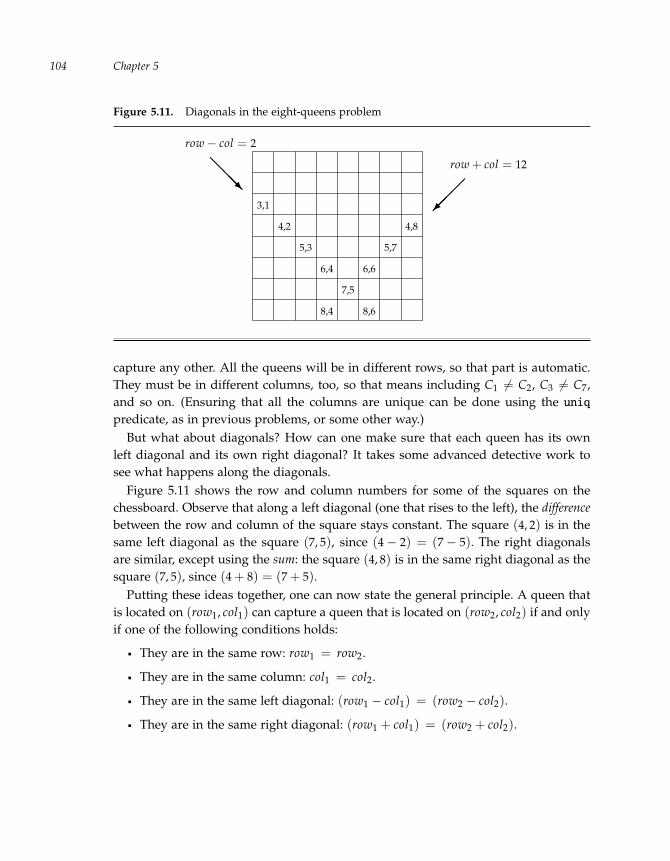
“run” — 2011/9/8 — 18:05 — page 104 — #127�

�

�

�

�

�

�

�

Chapter 5104

Figure 5.11. Diagonals in the eight-queens problem

��

��

row + col = 12

row − col = 2

3,1

4,2

5,3

6,4

7,5

8,6

4,8

5,7

6,6

8,4

capture any other. All the queens will be in different rows, so that part is automatic.They must be in different columns, too, so that means including C1 �= C2, C3 �= C7,and so on. (Ensuring that all the columns are unique can be done using the uniqpredicate, as in previous problems, or some other way.)

But what about diagonals? How can one make sure that each queen has its ownleft diagonal and its own right diagonal? It takes some advanced detective work tosee what happens along the diagonals.

Figure 5.11 shows the row and column numbers for some of the squares on thechessboard. Observe that along a left diagonal (one that rises to the left), the differencebetween the row and column of the square stays constant. The square (4, 2) is in thesame left diagonal as the square (7, 5), since (4 − 2) = (7 − 5). The right diagonalsare similar, except using the sum: the square (4, 8) is in the same right diagonal as thesquare (7, 5), since (4 + 8) = (7 + 5).

Putting these ideas together, one can now state the general principle. A queen thatis located on (row1, col1) can capture a queen that is located on (row2, col2) if and onlyif one of the following conditions holds:

They are in the same row: row1 = row2.

They are in the same column: col1 = col2.

They are in the same left diagonal: (row1 − col1) = (row2 − col2).

They are in the same right diagonal: (row1 + col1) = (row2 + col2).

“run” — 2011/9/8 — 18:05 — page 105 — #128�

�

�

�

�

�

�

�


Figure 5.12. Testing if one queen can capture another cap.pl

% cap(r1,C1,E2,C2) tests if a queen placed on an 8x8 chess board

% at position (R1,C1) can capture another at position (R2,C2).

cap(R,_,R,_). % Note the use of the _ here

cap(_,C,_,C). % and here, too.

cap(R1,C1,R2,C2) :- R1-C1 =:= R2-C2.

cap(R1,C1,R2,C2) :- R1+C1 =:= R2+C2.

Figure 5.13. A solution to the eight-queens problem queens.pl

% Solve the 8-queens problem.

solution(C1,C2,C3,C4,C5,C6,C7,C8) :-

col(C1),

col(C2), \+ cap(2,C2,1,C1),

col(C3), \+ cap(3,C3,1,C1), \+ cap(3,C3,2,C2),

col(C4), \+ cap(4,C4,1,C1), \+ cap(4,C4,2,C2), \+ cap(4,C4,3,C3),


\+ cap(5,C5,4,C4),


\+ cap(6,C6,4,C4), \+ cap(6,C6,5,C5),


\+ cap(7,C7,4,C4), \+ cap(7,C7,5,C5), \+ cap(7,C7,6,C6),


\+ cap(8,C8,4,C4), \+ cap(8,C8,5,C5), \+ cap(8,C8,6,C6),

\+ cap(8,C8,7,C7).

% The columns

col(1). col(2). col(3). col(4). col(5). col(6). col(7). col(8).

% cap(R1,C1,R2,C2): a queen on (R1,C1) can capture one on (R2,C2).

cap(R,_,R,_). % Note the use of the _ here

cap(_,C,_,C). % and here, too.

cap(R1,C1,R2,C2) :- R1-C1 =:= R2-C2.

cap(R1,C1,R2,C2) :- R1+C1 =:= R2+C2.

Before writing the solution predicate for this problem, it is a good idea to writethe clauses for a predicate cap(r1, c1, r2, c2), which holds when a queen placed on(r1, c1) can capture one that is placed on (r2, c2). The predicate will need four clausesthat mirror the four conditions. The resulting small program is shown in figure 5.12.(Always test that an auxiliary predicate like cap is working properly before includingit in a larger program.)

“run” — 2011/9/8 — 18:05 — page 106 — #129�

�

�

�

�

�

�

�

Chapter 5106

Figure 5.14. Running the eight-queens program

?- solution(C1,C2,C3,C4,C5,C6,C7,C8).

C1 = 1, C2 = 5, C3 = 8, C4 = 6

C5 = 3, C6 = 7, C7 = 2, C8 = 4

QQ

QQ

QQ

QQ

The complete solution predicate for the eight-queens problem is shown infigure 5.13. It says that a solution is generated as follows:

1. Generate a column for the queen in row 1 using col.

2. Generate a column for the queen in row 2 using col, and then test using cap thatthis queen cannot capture the one in row 1.

3. Generate a column for the queen in row 3 using col, and then test using cap thatthis queen cannot capture the one in row 1 nor the one in row 2.

4. Generate a column for the queen in row 4 using col, and then test using cap thatthis queen cannot capture the one in row 1, row 2, or row 3.

5. Continue in this way for row 5, row 6, row 7, and row 8.

Note how the negation of the cap predicate is used at each stage.There are many arrangements of the queens on a chessboard that will satisfy all the

constraints. The first one found by the solution predicate is displayed in figure 5.14.It is worth noting that because of how the col predicate is defined, this programalways tries columns in numeric order, 1, 2, 3, and so on. So not surprisingly, thefirst solution has a queen on (1,1). However, it does not have a queen on (2,3). Thismeans that although a queen on (2,3) is safe from the queen on (1,1), there is no wayto place the remaining six queens safely if one starts with (1,1) and (2,3). Similarly, aqueen on (2,4) leads to a dead end, and (2,5) is the first choice for the second queenthat works with the remaining six queens. Then for the third queen, the (3,2) and (3,7)positions would be safe, but again this would not allow the remaining five queensto be positioned safely, and so (3,8) is the first choice that works with the rest of thequeens.

“run” — 2011/9/8 — 18:05 — page 107 — #130�

�

�

�

�

�

�

�


Given the amount of searching and backtracking required to properly place queenson even an 8 × 8 board, computer scientists have looked for more efficient ways ofsolving this problem. One method that works well involves placing the queens ran-domly on a board and then repeatedly moving one of the queens to reduce its conflictswith the others.

5.5 A fourth example: Logic problems

This section considers a very different sort of puzzle, often called a logic problem,although it is no more connected to logic than the others. It is a word problem involv-ing several clues about the identities of individuals playing certain roles. A simpleexample illustrates the form:

In conversation, Sandy, Chris, and Pat discovered that they had distinct occupa-tions and also played distinct musical instruments. Their occupations are doctor,lawyer, and engineer, and the instruments they play are piano, flute, and violin.Also,

1. Chris is married to the doctor.

2. The lawyer plays the piano.

3. Chris is not the engineer.

4. Sandy is a patient of the violinist.

Who plays the flute?

To solve logic puzzles like these as constraint satisfaction problems, one needs todetermine what the variables are, what the domains should be, and how the giveninformation leads to constraints on the desired solution.

For this example, to determine who plays the flute, it is necessary to figure outwho (among Sandy, Chris, and Pat) plays what instrument and has what job. So theproblem can be characterized as follows:

Variables: Doctor, Lawyer, Engineer, Piano, Violin, Flute

Domain: {sandy, chris, pat}To encode the given information as constraints, these two implicit facts mustsomehow be included:

If x is married to y, then x �= y.

If x is a patient of y, then x �= y and y is the doctor.

“run” — 2011/9/8 — 18:05 — page 108 — #131�

�

�

�

�

�

�

�

Chapter 5108

Figure 5.15. A solution to the first logic problem logic1.pl

% A logic puzzle involving jobs and musical instruments,

solution(Flute) :-

% Distinct occupations and instruments

uniq_people(Doctor,Lawyer,Engineer),

uniq_people(Piano,Violin,Flute),

% The four clues

\+ chris = Doctor, % Chris is married to the doctor.

Lawyer = Piano, % The lawyer plays the piano.

\+ Engineer = chris, % The engineer is not Chris.

Violin = Doctor, % Sandy is a patient of

\+ sandy = Violin. % the violinist.

% uniq(...) is used to generate three distinct people.

uniq_people(A,B,C) :- person(A), person(B), person(C),

\+ A=B, \+ A=C, \+ B=C.

% The three given people

person(chris). person(sandy). person(pat).

Putting such facts into a knowledge base is tricky, since the conclusions involve equal-ity. For present purposes, it is much easier to embed the information directly in thesolution predicate, as shown in figure 5.15. The rest of the program is similar toprevious examples.

5.5.1 Hidden variables

The main challenge in logic problems like these is typically to determine how toexpress the constraints. Often the only way to do this is to imagine that there arehidden variables that are not mentioned but whose values need to be taken into account.This was the case with the carry digits in the cryptarithmetic problems. They had tobe introduced in order to express the constraints among the mentioned digits.

For example, suppose there is exactly the same logic problem as before, except thatconstraint 3 is

3. Pat is not married to the engineer.

How should this piece of information be handled? At first it seems that it places noconstraint on either Pat or the engineer. However, it is useful to think in terms of newvariables, for Pat’s spouse, Chris’s spouse, and Sandy’s spouse. Assuming they canonly be married to each other, the domain for these variables will be the three people(sandy, chris, pat) or none, to handle the case where the person is not married. The

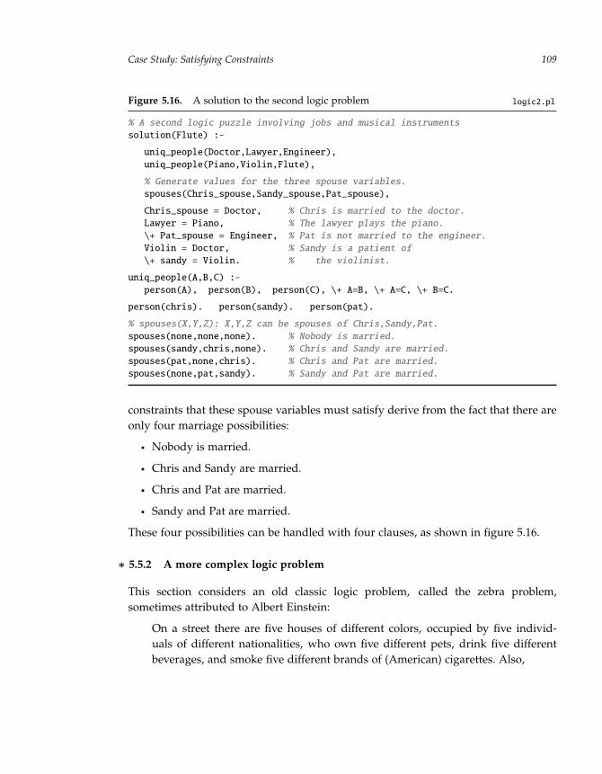
“run” — 2011/9/8 — 18:05 — page 109 — #132�

�

�

�

�

�

�

�


Figure 5.16. A solution to the second logic problem logic2.pl

% A second logic puzzle involving jobs and musical instruments

solution(Flute) :-

uniq_people(Doctor,Lawyer,Engineer),

uniq_people(Piano,Violin,Flute),

% Generate values for the three spouse variables.

spouses(Chris_spouse,Sandy_spouse,Pat_spouse),

Chris_spouse = Doctor, % Chris is married to the doctor.

Lawyer = Piano, % The lawyer plays the piano.

\+ Pat_spouse = Engineer, % Pat is not married to the engineer.

Violin = Doctor, % Sandy is a patient of

\+ sandy = Violin. % the violinist.

uniq_people(A,B,C) :-

person(A), person(B), person(C), \+ A=B, \+ A=C, \+ B=C.

person(chris). person(sandy). person(pat).

% spouses(X,Y,Z): X,Y,Z can be spouses of Chris,Sandy,Pat.

spouses(none,none,none). % Nobody is married.

spouses(sandy,chris,none). % Chris and Sandy are married.

spouses(pat,none,chris). % Chris and Pat are married.

spouses(none,pat,sandy). % Sandy and Pat are married.

constraints that these spouse variables must satisfy derive from the fact that there areonly four marriage possibilities:

Nobody is married.

Chris and Sandy are married.

Chris and Pat are married.

Sandy and Pat are married.

These four possibilities can be handled with four clauses, as shown in figure 5.16.

∗ 5.5.2 A more complex logic problem

This section considers an old classic logic problem, called the zebra problem,sometimes attributed to Albert Einstein:

On a street there are five houses of different colors, occupied by five individ-uals of different nationalities, who own five different pets, drink five differentbeverages, and smoke five different brands of (American) cigarettes. Also,

“run” — 2011/9/8 — 18:05 — page 110 — #133�

�

�

�

�

�

�

�

Chapter 5110

1. The occupant of the red house is English.

2. The Spaniard owns a dog.

3. The coffee drinker lives in a green house.

4. The Ukrainian drinks tea.

5. The ivory house is to the left of the green one.

6. The snail owner smokes Winstons.

7. The person in the yellow house smokes Kools.

8. The occupant in the middle house drinks milk.

9. The Norwegian lives in the leftmost house.

10. The Chesterfield smoker lives next to the fox owner.

11. The Kool smoker lives next to the horse owner.

12. The orange juice drinker smokes Lucky Strikes.

13. The Parliament smoker is Japanese.

14. The Norwegian lives next to a blue house.

Who owns the zebra?

Observe that most of these clues will end up being statements of equality among thevariables:

4. The Ukrainian drinks tea.Ukrainian = TeaDrinker

6. The snail owner smokes Winstons.SnailOwner = WinstonSmoker

The question is what to do about the constraints involving position:

5. The ivory house is to the left of the green one.

(Note that left here means directly to the left.) This fact needs to relate to otherpositional constraints like the following:

8. The occupant in the middle house drinks milk.

9. The Norwegian lives in the leftmost house.

10. The Chesterfield smoker lives next to the fox owner.

First determine what domain to use for the variables. As long as the appropriate equal-ity and inequality constraints are enforced, the values can be taken from any set. The

“run” — 2011/9/8 — 18:05 — page 111 — #134�

�

�

�

�

�

�

�


Figure 5.17. A solution to the zebra problem zebra.pl

% This is a solution to the classic zebra puzzle.

solution(Zebra,England,Spain,Ukraine,Japan,Norway) :-

% The fourteen clues

England=Red, Spain=Dog, Coffee=Green, Ukraine=Tea,

left(Ivory,Green), Winston=Snail, Kool=Yellow,

middle_pos(Milk), leftmost_pos(Norway),

next_to(Chesterfield,Fox), next_to(Kool,Horse),

LuckyStrike=OJ, Japan=Parliament, next_to(Norway,Blue),

% The five lists: houses, nations, pets, drinks, cigarettes

uniq_pos(Green,Red,Yellow,Ivory,Blue),

uniq_pos(England,Spain,Ukraine,Japan,Norway),

uniq_pos(Dog,Snail,Zebra,Fox,Horse),

uniq_pos(Tea,Milk,OJ,Coffee,OtherDrink),

uniq_pos(Winston,Kool,Parliament,Chesterfield,LuckyStrike).

%-------------- The positional predicates -------------------

uniq_pos(P1,P2,P3,P4,P5) :-

pos(P1), pos(P2), pos(P3), pos(P4), pos(P5),

\+ P1=P2, \+ P1=P3, \+ P1=P4, \+ P1=P5, \+ P2=P3,

\+ P2=P4, \+ P2=P5, \+ P3=P4, \+ P3=P5, \+ P4=P5.

pos(1). pos(2). pos(3). pos(4). pos(5).

leftmost_pos(1). middle_pos(3).

left(1,2). left(2,3). left(3,4). left(4,5).

next_to(X,Y) :- left(X,Y).

next_to(X,Y) :- left(Y,X).

positional constraints suggest that values be taken from a positional ordering of the fivehouses: 1 (leftmost), 2 (left middle), 3 (middle), 4 (right middle), 5 (rightmost). Theknowledge base can include facts about which position is leftmost, which is middle,which position is directly to the left of another, and which position is next to another.These positional facts together with the clause for the solution predicate (from thefourteen puzzle clues and the uniqueness constraints) are shown in figure 5.17.

Since the values of all the variables are just positional numbers, it takes some extrawork to get a more descriptive answer. A query with the solution predicate bringsthe following result:

?- solution(Zebra,E,S,U,J,N).

Zebra = 5, E = 3, S = 4, U = 2, J = 5, N = 1

Yes

“run” — 2011/9/8 — 18:05 — page 112 — #135�

�

�

�

�

�

�

�

Chapter 5112

Figure 5.18. A scheduling problem

The task is to schedule a new class to meet five hours each week.

Meeting times are on the hour from 9am to 4pm, on weekdays.

Some of the periods will be taken by previously scheduled activities.

Classes must not meet on successive hours on the same day, or formore than two hours total on any one day.

This says that the zebra is in house 5, the rightmost house. But who lives there? Tofind out, use a print_solution predicate defined as follows:

print_solution :-

solution(Zeb,E,S,U,J,N), pmatch(Zeb,E,’English’),

pmatch(Zeb,S,’Spanish’), pmatch(Zeb,U,’Ukrainian’),

pmatch(Zeb,J,’Japanese’), pmatch(Zeb,N,’Norwegian’).

pmatch(X,X,Name) :- % Write when there is a match.

nl, write(’The zebra owner is ’), write(Name).

pmatch(X,Y,Name) :- \+ X=Y. % Write nothing in this case.

The print_solution predicate uses the positional information to print the nationalitythat matches the zebra house number:

?- print_solution.

The zebra owner is Japanese

∗ 5.6 A fifth example: Scheduling

The constraint satisfaction problem in this section is not a puzzle at all, but rather amuch more practical problem, scheduling. Examples of scheduling include assigningpeople to jobs, or meetings to rooms, or courses to final exam periods. Solving prob-lems like these still requires thinking of course, but now the thinking is not done justfor the fun of it, as with puzzles.

A scheduling problem involving the timetable for a course is shown in figure 5.18.The task is to find periods (that is, the days and times) for the five classes. This can beformulated as a constraint satisfaction problem as follows:

Variables: P1, P2, P3, P4, P5, where each Pi is a period for the course.

“run” — 2011/9/8 — 18:05 — page 113 — #136�

�

�

�

�

�

�

�


Domains: Each period is a certain time on a certain day. A period can be encodedas a number: (100 × day) + 24 hr. clock. So, for example, for Monday at 9am, theperiod would be 109; for Tuesday at 2pm, it would be 214; and for Friday at 4pm,it would be 516.

Constraints: The five chosen periods must be available (not already taken), non-consecutive, and with no more than two per day. In addition (although it is notstated explicitly), the five periods must all be distinct.

The following generates five available periods:

% P1,P2,P3,P4,P5 are five distinct available periods.

uniq_periods(P1,P2,P3,P4,P5) :-

per(P1), per(P2), per(P3), per(P4), per(P5),

\+ P1=P2, \+ P1=P3, \+ P1=P4, \+ P1=P5, \+ P2=P3,

\+ P2=P4, \+ P2=P5, \+ P3=P4, \+ P3=P5, \+ P4=P5.

% per(P): P is a period that is not already taken.

per(P) :- day(D), time(T), P is 100*D+T, \+ taken(P).

day(1). day(2). day(3). day(4). day(5). % The five days

time(9). time(10). time(11). time(12). % The eight times

time(13). time(14). time(15). time(16).

This assumes that the taken predicate is defined separately to tell which periods havebeen taken by previously scheduled activities.

The solution predicate for this scheduling problem is shown in figure 5.19. Theconstraints are handled by two predicates: not_2_in_a_row ensures that there isnot a pair of periods where one is an hour earlier or later than the other; andnot_3_same_day ensures that there are not three periods that are on the same day.(The day of a period is obtained by doing integer division by 100.)

All that remains is to specify which periods are unavailable using the taken pred-icate. An example specification appears in figure 5.20. Adding those clauses to thescheduling program gives the following:

?- solution(P1,P2,P3,P4,P5).

P1 = 111, P2= 113, P3 = 213, P4 = 409, P5 = 411

% Mon 11am Mon 1pm Tue 1pm Thu 9am Thu 11am

The scheduling constraints are somewhat loose in this example, so the solutiondisplayed here is not unique.

“run” — 2011/9/8 — 18:05 — page 114 — #137�

�

�

�

�

�

�

�

Chapter 5114

Figure 5.19. A classroom scheduler schedule-top.pl

% This program solves a classroom scheduling problem.

solution(P1,P2,P3,P4,P5) :-

uniq_periods(P1,P2,P3,P4,P5), % All different periods.

not_2_in_a_row(P1,P2,P3,P4,P5), % Not two consecutive hrs.

not_3_same_day(P1,P2,P3,P4,P5). % Not three on the same day.

not_2_in_a_row(P1,P2,P3,P4,P5) :-

\+ seq(P1,P2), \+ seq(P1,P3), \+ seq(P1,P4), \+ seq(P1,P5),

\+ seq(P2,P3), \+ seq(P2,P4), \+ seq(P2,P5), \+ seq(P3,P4),

\+ seq(P3,P5), \+ seq(P4,P5).

seq(A,B) :- A =:= B-1.

seq(A,B) :- A =:= B+1.

not_3_same_day(P1,P2,P3,P4,P5) :-

\+ eqday(P1,P2,P3), \+ eqday(P1,P2,P4), \+ eqday(P1,P2,P5),



\+ eqday(P3,P4,P5).

eqday(A,B,C) :- Z is A // 100, Z is B // 100, Z is C // 100.

% The definition of uniq_periods is elsewhere.

Figure 5.20. Previously scheduled periods schedule-aux.pl

% Monday: only 11am and 1pm are available.

taken(X) :- X // 100 =:= 1, \+ X=111, \+ X=113.

% Tuesday: only 1pm and 2pm are available.

taken(X) :- X // 100 =:= 2, \+ X=213, \+ X=214.

% Wednesday: nothing available.

taken(X) :- X // 100 =:= 3.

% Thursday: all available, except for 10am, 12pm, and 2pm.

taken(410). taken(412). taken(414).

% Friday: nothing available.

taken(X) :- X // 100 =:= 5.

Want to read more?

This chapter was about the thinking required to solve constraint satisfaction problems.As noted, the subarea of AI called constraint programming studies how to do thisefficiently. Work in this area began in the 1970s when Montanari [27] and Mackworth

“run” — 2011/9/8 — 18:05 — page 115 — #138�

�

�

�

�

�

�

�


[26] first formulated constraint satisfaction problems in the form considered here.They also proposed methods of solving them that appear to work much better inpractice than generate-and-test. An excellent graduate-level textbook about this areaof research is by Dechter [24]. (Note: Scheduling has a history of its own outside ofcomputer science in the area of operations research.)

Constraint satisfaction is connected to many areas of computer science, for example,answering queries in databases [28]. As it turns out, it also raises a very fundamentalquestion about computation itself. To take Sudoku as an example, each Sudoku puzzleis of size n2 × n2 for some n (like 9 × 9 or 121 × 121), and the search space grows veryquickly, in fact, exponentially with n. The question is whether there is a way to solvethese puzzles that is guaranteed to do better than generate-and-test over this enormousspace.

This question can be reformulated in a mathematically precise way using the notionof a Turing machine (mentioned at the end of chapter 1). Is there a Turing machine Mand a polynomial P such that M can solve any Sudoku puzzle of size n2 ×n2 (or reportthat there is no solution) in no more than P(n) steps? The answer, remarkably enough,is that nobody knows. The question is equivalent to the famous P=NP question, firstposed by Stephen Cook [23] in the 1970s, and despite the best efforts of thousandsof computer scientists and mathematicians since then, it has remained unanswered.Anyone who can answer it will become instantly famous and receive a $1 millionreward from the Clay Mathematics Institute. What is known about the question isthat no matter how the answer turns out, it will affect the view of thousands of othercomputational tasks, some of which have direct economic significance [25].

Exercises

1. This chapter presented three different ways of handling equality in Prolog: =,=:=, and is. For each of the three, explain briefly what its purpose is, andpresent an example setting where it should be used but where the other twoshould not be used.

2. Draw a map of central Europe consisting of the following seven countries: France,Switzerland, Italy, Belgium, Holland, Germany, and Austria. Color the countrieson the map using just red, yellow, and orange; no two countries with a borderbetween them can be the same color. Look at an existing map to see where theborders are, and then write a Prolog program that will find a color for eachcountry.

“run” — 2011/9/8 — 18:05 — page 116 — #139�

�

�

�

�

�

�

�

Chapter 5116

3. Use Prolog to solve the cryptarithmetic puzzle CROSS + ROADS = DANGER.Note: If you are not careful with the ordering of constraints in your program,the program could run for hours. With a proper ordering, it should only take asecond or so. Explain briefly the order you have chosen.

4. Consider the following problem:

Donna, Danny, David, and Doreen were seated at a table in a restaurant.The men sat across from each other, as did the women. They each ordered adifferent main course with a different beverage. In addition,

– Doreen sat beside the person who ordered steak.

– The chicken came with a Coke.

– The person with the lasagna sat across from the person with milk.

– David never drinks coffee.

– Donna only drinks water.

– Danny could not afford to order steak.

Who ordered the pizza?

Write a Prolog program that solves this problem by displaying who ordered eachof the main courses and each of the beverages. Hint: Begin by writing clausesdefining predicates beside(x, y), which holds if person x is sitting beside persony, and across(x, y), which holds if person x is sitting across from person y.

5. Many newspapers feature a puzzle called KenKen in the recreational section.The KenKen puzzle is similar to Sudoku except that arithmetic relations areinvolved. Write a Prolog program that solves a 4 × 4 KenKen puzzle taken froma newspaper.

Hint: You will need the uniq predicate used for the Sudoku problem for the rowsand for the columns. It will also be convenient to define two auxiliary predicates,sub and div, where sub(x, y, z) holds when either z = x − y or z = y − x, anddiv(x, y, z) holds when either z = x ÷ y or z = y ÷ x.

6. The answers submitted by five students to a true/false quiz are as follows:

Teresa: true, true, false, true, falseTim: false, true, true, true, falseTania: true, false, true, true, falseTom: false, true, true, false, trueTony: true, false, true, false, true

“run” — 2011/9/8 — 18:05 — page 117 — #140�

�

�

�

�

�

�

�


Tania got more answers right than Teresa did. Tom got more right than Tim. Tonydid not get all the answers right, nor did he get them all wrong. Write a Prologprogram to find the correct answers to the quiz.

Hint: Write a predicate grade(s1, s2, s3, s4, s5, a1, a2, a3, a4, a5, n) that holds when nis the number of correct answers when a student submits the si, and the correctanswers are the ai. (So grade counts the matches between the si and ai.)

7. Consider a course timetable for a Fine Arts student at a mythical university.The student wants to take a course in art, music, film, and dance, and each ofthese has three hours of classes a week. To accommodate a variety of timingconstraints, some courses offer two sections at different times.

There are two possible sections for art. One is offered MWF10, and the other,MWF11.

There is a single section of dance: Friday 1–4.

Music can be taken either Monday at 11, Wednesday at 3, and Friday at 3, orMonday at 2, Wednesday at 2, and Friday at 11.

There are two sections of film: one on Monday at 11, Wednesday at 11,and Friday at noon, and one on Monday at noon, Wednesday at noon, andWednesday at 3.

In addition, the student wants a free hour for lunch each day at noon or at 1.Write a Prolog program that generates a timetable for the student.

“run” — 2011/9/8 — 18:05 — page 118 — #141�

�

�

�

�

�

�

�

“run” — 2011/9/8 — 18:05 — page 119 — #142�

�

�

�

�

�

�

�

∗ 6 Case Study: Interpreting Visual Scenes

The previous chapter gave examples of the sort of thinking required to solve certainpuzzles. This type of thinking does have some distinctive features when done bypeople. It requires concentration and effort; memory aids (like pencil and paper) areusually helpful; some people are much better at it than others; and some people seeno fun in the activity at all.

In this chapter, the idea of constraint satisfaction is applied to a form of thinkingthat seems much more natural and relaxed: visual interpretation. This is a type ofthinking that everyone can do to some extent, typically with a lot less conscious effortthan puzzles require.

The first section briefly considers the concept of vision and its connection tothinking. The following sections examine a sampling of three visual interpretationtasks: the interpretation of an image of a two-dimensional terrain as seen fromabove (section 2); the interpretation of the edges in an image of three-dimensionalpolyhedral objects (section 3); and recognizing objects of interest in an image(section 4).

6.1 The thinking part of vision

What is vision? In its simplest terms, it is the process of identifying the physicalobjects around us by interpreting the patterns of light that reflect off them. Digitizingthe problem somewhat, one can rephrase it as follows. Imagine that a certain numberof times per second, our eyes are presented with an image, that is, a two-dimensionalgrid of picture elements (or pixels). The job of vision is to respond to these imageswith something like “German shepherd puppy” or “Jackson Pollock painting” or“delivery truck coming straight for me.” The exact details of the image and the desiredresponses need not concern us.

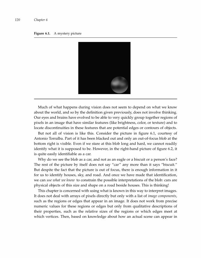
“run” — 2011/9/8 — 18:05 — page 120 — #143�

�

�

�

�

�

�

�

Chapter 6120

Figure 6.1. A mystery picture

Much of what happens during vision does not seem to depend on what we knowabout the world, and so by the definition given previously, does not involve thinking.Our eyes and brains have evolved to be able to very quickly group together regions ofpixels in an image that have similar features (like brightness, color, or texture) and tolocate discontinuities in these features that are potential edges or contours of objects.

But not all of vision is like this. Consider the picture in figure 6.1, courtesy ofAntonio Torralba. Part of it has been blacked out and only an out-of-focus blob at thebottom right is visible. Even if we stare at this blob long and hard, we cannot readilyidentify what it is supposed to be. However, in the right-hand picture of figure 6.2, itis quite easily identifiable as a car.

Why do we see the blob as a car, and not as an eagle or a biscuit or a person’s face?The rest of the picture by itself does not say “car” any more than it says “biscuit.”But despite the fact that the picture is out of focus, there is enough information in itfor us to identify houses, sky, and road. And once we have made that identification,we can use what we know to constrain the possible interpretations of the blob: cars arephysical objects of this size and shape on a road beside houses. This is thinking!

This chapter is concerned with using what is known in this way to interpret images.It does not deal with arrays of pixels directly but only with a list of image components,such as the regions or edges that appear in an image. It does not work from precisenumeric values for these regions or edges but only from qualitative descriptions oftheir properties, such as the relative sizes of the regions or which edges meet atwhich vertices. Then, based on knowledge about how an actual scene can appear in

“run” — 2011/9/8 — 18:05 — page 121 — #144�

�

�

�

�

�

�

�

Case Study: Interpreting Visual Scenes 121

Figure 6.2. The mystery picture revealed

Figure 6.3. An aerial sketch map

An aerial sketch map is depicted onthe left. The interpretation task isto identify each region of the imageas one of grass, water, pavement, ahouse, or a vehicle.

an image, the job is to interpret the image components, that is, to identify (at somelevel) what the regions or edges actually represent in the scene.

This visual interpretation can be formulated as a constraint satisfaction problem.However, considerably more knowledge of the world will have to be applied than forthe problems of chapter 5.

6.2 Aerial sketch maps

Imagine looking down from an airplane passing over a terrain and seeing the imagerepresented by the sketch in figure 6.3. The job is to identify the various regions in the

“run” — 2011/9/8 — 18:05 — page 122 — #145�

�

�

�

�

�

�

�

Chapter 6122

image. Here is the background knowledge one might expect to use to help identifythese regions:

A region cannot border or be surrounded by a region of the same type.

Houses cannot be next to or surrounded by water.

Vehicles must be next to or surrounded by pavement.

Pavement cannot be completely inside any other region.

Houses, vehicles, and pavement have regular shapes (with straight edges);grass and water have irregular shapes.

Vehicles are small; the other regions are large.

These statements constrain the permissible interpretations of regions that appear inimages in terms of size (large or small), shape (regular or irregular), borders (what isnext to what), and containment (what is surrounded by what). In reality, of course,there are many exceptions to these rules (like houseboats that are on water, and pavedtennis courts that are surrounded by grass), but these are ignored for now.

A Prolog program that captures these facts appears in figure 6.4. It describes what ispermissible in an image of this sort. For example, the query border(pavement,grass)returns success. This does not mean that an image must have a region of pavementnext to a region of grass but only that it could. The query border(water,vehicle),on the other hand, returns failure, which means that an image cannot portray a regionof water next to a vehicle.

6.2.1 Constraints on image regions

With this background knowledge about the scene, the image can now be interpreted.Start with a list of regions, along with the properties they have in the image, asin figure 6.5. Approach the visual interpretation task as a constraint satisfactionproblem:

The variables are the regions of the image: R1, R2, R3, R4, R5.

Each variable must take a value from one of the region types: grass, water,pavement, house, and vehicle.

The constraints that need to be satisfied are the image properties listed infigure 6.5, in conjunction with the background knowledge about the permissibleinterpretations of region types.

‘‘run’’ --- 2011/9/8 --- 18:05 --- page 123 --- #146�

�

�

�

�

�

�

�


Figure 6.4. The types of regions and their properties regions.pl

% The five types of regions that can appear in an image

region(grass). region(water). region(pavement).

region(house). region(vehicle).

% small(X) holds when region X can be small in an image.

small(vehicle).

% regular(X) holds when region X can be regular in an image.

regular(pavement). regular(house). regular(vehicle).

% border(X,Y) holds when region X can border region Y.

border(X,Y) :- \+ bad_border(X,Y), \+ bad_border(Y,X).

% Unacceptable borders

bad_border(X,X).

bad_border(house,water).

bad_border(vehicle,X) :- \+ X=pavement.

% inside(X,Y) holds when region X can be surrounded by Y.

inside(X,Y) :- \+ bad_inside(X,Y).

% Unacceptable containment

bad_inside(X,X).

bad_inside(house,water).

bad_inside(vehicle,X) :- \+ X=pavement.

bad_inside(pavement,_).

Figure 6.5. The image regions and their properties

R1

R2R3

R4R5

Region R5 is small;the others are large.

Region R3 and R5 are regular;R1 and R2 are irregular;R4 could go either way.

Region R1 borders on R2;R2 borders on R4.

Region R3 is inside R2;R5 is inside R4.

This leads to the solution predicate in Prolog that appears in figure 6.6. Loading thisprogram together with the one in figure 6.4 produces this behavior:

“run” — 2011/9/8 — 18:05 — page 124 — #147�

�

�

�

�

�

�

�

Chapter 6124

Figure 6.6. The sketch map interpretation sketch.pl

solution(R1,R2,R3,R4,R5) :-

region(R1), region(R2), region(R3), region(R4), region(R5),

% Size constraints

\+ small(R1), \+ small(R2), \+ small(R3),

\+ small(R4), small(R5),

% Regularity constraints (none for R4)

regular(R3), regular(R5), \+ regular(R2), \+ regular(R1),

% Border constraints

border(R1,R2), border(R2,R4),

% Containment constraints

inside(R3,R2), inside(R5,R4).

% The definitions of region, small, border, etc. are elsewhere.

?- solution(R1,R2,R3,R4,R5).

R1 = water, R2 = grass, R3 = house,

R4 = pavement, R5 = vehicle

This is the only visual interpretation that satisfies all the constraints. Note how theinterpretations for some regions help to disambiguate others. For example, R4 is large,so it cannot be a vehicle. But it is not clear whether it should be seen as regular orirregular. However, it clearly surrounds region R5, and once it is determined that R5 isa vehicle, background knowledge leads to the conclusion that R4 must be pavement.On a much smaller scale, this is precisely the sort of thinking that took place tointerpret the blob as a car in figure 6.2!

Also note that the constraints work together to identify the regions and that therecan be redundancy. For example, if the \+ small(R3) constraint is eliminated fromthe solution predicate, one still gets a unique interpretation of the image as before.This is why it was not necessary to specify whether region R4 was regular or irregularin the image. On the other hand, if the small(R5) constraint were eliminated instead,there would be two interpretations: the previous one and a second one where R5 isa house. Of course, if the constraint \+ small(R1) were replaced by small(R1), theimage would have no interpretation at all.

6.3 Polyhedral objects

Figure 6.7 shows a very different type of image, a three-dimensional, L-shaped, block-like object (or polyhedron). At first, it is not clear that any interpretation is needed here.

“run” — 2011/9/8 — 18:05 — page 125 — #148�

�

�

�

�

�

�

�


Figure 6.7. A polyhedral object and its labels

A

B

C

D

E F

G

H

I

J

K

+

-

+

+

+

+

+

��

�

�

�

�

�

But consider the five horizontal lines that appear in the image. Part of making senseof this image is realizing that these lines do not all mean the same thing:

The top horizontal line is a boundary of the object. The viewer understands thatjust below the line is a face of the object, and just above the line is empty space(unless the object is up against a wall).

The bottom horizontal line is also a boundary of the object. But this time thespace just above the line is part of the object, and just below the line is emptyspace (unless the object is on top of another).

The middle horizontal line represents the intersection of two faces of the object.Moreover, the intersection is concave (or hinged inward, like the letter V as seenfrom above).

The two remaining horizontal lines also represent the intersection of two faces ofthe object. In these cases, however, the intersection is convex (or hinged outward,like the letter V as seen from below).

Interpreting an image of a polyhedral object involves labeling each edge in this way.The image at the right in figure 6.7 shows the vertices named and the edges labeled:+ for a convex edge, - for a concave edge, and an arrow for a boundary edge with asurface to the right relative to its direction. The edge AH is labeled < meaning thatin going from A to H the surface is to the left. Of course, there is nothing inherentlydirectional in the edges of an image. So the reverse edge HA should be understood

“run” — 2011/9/8 — 18:05 — page 126 — #149�

�

�

�

�

�

�

�

Chapter 6126

Figure 6.8. The four vertex types

Arrow

��

Fork

��

L-vertex

��

T-vertex

as labeled >, since in going from H to A the surface is to the right. (The + and - labelswill be the same for either direction of the edge.)

6.3.1 Constraints on vertices and edges

What kind of background knowledge is expected in order to interpret edges in animage like this? The answer has to do with the vertices, where the edges meet. Onlyfour types of vertices are expected in such an image, as shown in figure 6.8. (All butthe T-vertex appear in figure 6.7: E, A, and G are L-vertices; C, K, and I are forks; therest are arrows.) Furthermore, in any polyhedral image, only some combinations ofedge types can meet at a vertex.

Consider, for example, the L-vertex of figure 6.8. Suppose that both edges meetingat the vertex were labeled +. Then because of the surfaces below each edge, therewould need to be an extra edge where they meet, making the vertex into an arrow.The conclusion: two edges labeled + cannot meet at an L-vertex.

The full range of possibilities for the edges at each type of vertex are shown infigure 6.9. These facts can be encoded in Prolog in a straightforward way, as is donein figure 6.10. In all cases, the edges are understood as leaving the vertex. The reversepredicate is used to relate the label of an edge to the label of the same edge in thereverse direction.

With this background knowledge, the visual interpretation of a polyhedral imagecan proceed. Given is a list of vertices, their types, and the edges that leave eachvertex. The job is to assign labels to each edge; this is approached as a constraintsatisfaction problem:

The variables are the edges in the image.

Each variable takes a value from one of the four labels: >, <, +, and -.

The constraints are that each vertex in the image must connect edges with labelsthat are in accordance with the rules shown in figure 6.9.

“run” — 2011/9/8 — 18:05 — page 127 — #150�

�

�

�

�

�

�

�


Figure 6.9. Permissible vertices in polyhedral images

��

��

-

++��

��

��

+

--��

��

+

��

��

+

++��

��

��-

-- ��

��

-

��

��

��-

�

��

�� -

� �

��

��

�� - ��

��

��

��

�� +��

��

-��

��

+

Figure 6.10. Permissible vertices in Prolog polyrules.pl

% All edges are assumed to leave the vertex in question.

% arrow(left,bottom,right)

arrow(’+’,’-’,’+’). arrow(’-’,’+’,’-’). arrow(’<’,’+’,’>’).

% fork(left,top,right)

fork(’+’,’+’,’+’). fork(’-’,’-’,’-’). fork(’>’,’-’,’<’).

fork(’-’,’<’,’>’). fork(’<’,’>’,’-’).

% tvertex(left,bottom,right)

tvertex(’>’,_,’<’).

% lvertex(left,right)

lvertex(’<’,’>’). lvertex(’<’,’-’). lvertex(’>’,’<’).

lvertex(’>’,’+’). lvertex(’-’,’>’). lvertex(’+’,’<’).

% Reversing the direction of an edge: only < and > change.

reverse(’+’,’+’). reverse(’-’,’-’).

reverse(’<’,’>’). reverse(’>’,’<’).

For the L-shaped object of figure 6.7, the solution predicate is shown in figure 6.11.There are fifteen arguments, corresponding to the fifteen edges in the image. Thefirst eleven atoms in the body correspond to the eleven vertices in the image. Note

“run” — 2011/9/8 — 18:05 — page 128 — #151�

�

�

�

�

�

�

�

Chapter 6128

Figure 6.11. Interpreting the edges in figure 6.7 polyinterp.pl

solution(AB,BC,CD,DE,EF,FG,GH,HA,HI,IB,IJ,JC,JK,KD,KF) :-

lvertex(AH,AB), arrow(BA,BI,BC), fork(CB,CD,CJ),

arrow(DC,DK,DE), lvertex(ED,EF), arrow(FE,FK,FG),

lvertex(GF,GH), arrow(HG,HI,HA), fork(IH,IB,IJ),

arrow(JK,JC,JI), fork(KD,KF,KJ),

reverse(AB,BA), reverse(BC,CB), reverse(CD,DC),

reverse(DE,ED), reverse(EF,FE), reverse(FG,GF),

reverse(GH,HG), reverse(HA,AH), reverse(HI,IH),

reverse(IB,BI), reverse(IJ,JI), reverse(JC,CJ),

reverse(JK,KJ), reverse(KD,DK), reverse(KF,FK).

print_lshape_interpretation :-

solution(AB,BC,CD,DE,EF,FG,GH,HA,HI,IB,IJ,JC,JK,KD,KF), nl,

write(AB), write(BC), write(CD), write(DE), write(EF),

write(FG), write(GH), write(HA), write(HI), write(IB),

write(IJ), write(JC), write(JK), write(KD), write(KF).

that in each case the edge leaving the vertex is used. For vertex A, for example,lvertex(AH,AB) is used, and not lvertex(HA,AB) or lvertex(AH,BA). (Since an edgeconnects two vertices, each direction of the edge will be used exactly once in theeleven atoms.) Loading this program together with the one in figure 6.10 producesthe following behavior:

?- print_lshape_interpretation.

>>>>>>>>+++-+++ ;

>>>>-->>+++-+++ ;

---->>>>+++-+++ ;

>>>>>>--+++-+++ ;

No

So four visual interpretations are found. These are shown graphically in figure 6.12.They all agree on the internal edges HI, IB, IJ, JC, JK, KD, and KF. The first interpreta-tion (top left of figure 6.12) is the one depicted in figure 6.7, where all the remainingedges are boundaries. In the next interpretation (top right of figure 6.12), the objectis seen as up against a wall (or another object) behind it, with EF and FG as concaveedges between two surfaces. In the third interpretation (bottom right), the object isseen as against a wall on the left, with AB, BC, CD, and DE as concave. Finally, in thelast interpretation (bottom left), the object is seen as resting on another, with GH andHA as concave. Note that if the edge BC is concave (as in figure 6.12, bottom right),the edges AB, CD, and DE cannot be boundaries; they, too, must be concave. Note

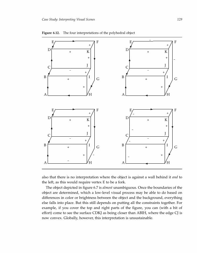
“run” — 2011/9/8 — 18:05 — page 129 — #152�

�

�

�

�

�

�

�


Figure 6.12. The four interpretations of the polyhedral object

A

B

C

D

E F

G

H

I

J

K

+

-

+

+

+

+

+

��

�

�

�

�

�

A

B

C

D

E F

G

H

I

J

K

+

-

+

+

+

+

+

��

�

-

�

�

�

-

A

B

C

D

E F

G

H

I

J

K

+

-

+

+

+

+

+

�-

-

�

-

-�

A

B

C

D

E F

G

H

I

J

K

+

-

+

+

+

+

+

-�

�

-

�

�

�

also that there is no interpretation where the object is against a wall behind it and tothe left, as this would require vertex E to be a fork.

The object depicted in figure 6.7 is almost unambiguous. Once the boundaries of theobject are determined, which a low-level visual process may be able to do based ondifferences in color or brightness between the object and the background, everythingelse falls into place. But this still depends on putting all the constraints together. Forexample, if you cover the top and right parts of the figure, you can (with a bit ofeffort) come to see the surface CDKJ as being closer than ABIH, where the edge CJ isnow convex. Globally, however, this interpretation is unsustainable.

“run” — 2011/9/8 — 18:05 — page 130 — #153�

�

�

�

�

�

�

�

Chapter 6130

Figure 6.13. A polyhedral object and an impossible variant

��

��

��

��

��

��

��

��

��

��

��

��

��

��

6.3.2 Impossible objects

This idea of images having only local interpretations is at the root of so-called impossi-ble objects. Consider figure 6.13. The image on the left is somewhat unusual but can beinterpreted as an object with two 90◦ turns. The one on the right (due to Roger Pen-rose), however, cannot be interpreted as a polyhedral object at all. By covering partsof the figure it is possible to interpret the rest of the figure in one way or another. Indoing visual interpretation, however, it is necessary to look for local cues and to tryto assemble a global interpretation that accounts for everything that is seen.

6.4 Object recognition

Given an image of some sort, the task of object recognition is to determine whetherthe image contains a depiction of a particular object, say, a door that is an exit, or abanquet table with food on it, or a parcel to pick up for delivery. This is the sort ofperceptual task that we do all the time, and it is absolutely crucial when we arrive ata new location. It is also somewhat different from the visual interpretation discussedin the previous sections. Rather than interpreting all the image elements, the goal isto pick out elements in the image corresponding to the kind of object being sought.

Here is a simple case. The image given is like the one in figure 6.14 and the job isto see if there is a cuboid (a rectangular-shaped block) in the image. As shown in thefigure, a list of vertices in the image is given (of the four types mentioned in the pre-vious section) together with the vertices to which they connect. The predicates from

“run” — 2011/9/8 — 18:05 — page 131 — #154�

�

�

�

�

�

�

�


Figure 6.14. An image with a cuboid and a wedge

5

6

7

4

1

2

3

8

9

10

11

12��

��

img_fork(1,2,4,6).

img_arr(6,5,1,7). img_arr(2,7,1,3). img_arr(4,3,1,5).

img_arr(9,8,11,10). img_arr(11,12,9,8).

img_lv(3,2,4). img_lv(5,4,6). img_lv(7,6,2).


Figure 6.15. Finding a cuboid in an image cuboid.pl

% A 3D view of a cuboid (seven vertices)

cuboid(A,B,C,D,E,F,G) :-

calc_arr(A,F,G,B), calc_lv(B,A,C), calc_arr(C,B,G,D),

calc_lv(D,C,E), calc_arr(E,D,G,F), calc_lv(F,E,A),

calc_fork(G,A,C,E).

% Vertex V, then left, mid, and right vertices

calc_arr(V,V1,V2,V3) :- img_arr(V,V1,V2,V3).

% Vertex V, then left and right vertices

calc_lv(V,V1,V2) :- img_lv(V,V1,V2).

% Vertex V, then the vertices in clockwise order

calc_fork(V,V1,V2,V3) :- img_fork(V,V1,V2,V3).



the image img_lv, img_arr, img_fork, and img_tv represent an L-vertex, an arrow,a fork, and a T-vertex, respectively. For example, img_arr(9,8,11,10) indicates thatvertex 9 in the image is an arrow vertex, with vertex 8 on its left branch, vertex 11 onits middle branch, and vertex 10 on the right. The task is to locate a cuboid withinthis collection of vertices.

What the cuboid predicate needs to do is to find a pattern of vertices that connectin a certain way. The Prolog code for this appears in figure 6.15. (The predicates

“run” — 2011/9/8 — 18:05 — page 132 — #155�

�

�

�

�

�

�

�

Chapter 6132

calc_arr, calc_lv, and calc_fork are used rather than the img predicates directly,since they will be refined later.) Loading this program and including the image datafrom figure 6.14 produces

?- cuboid(A,B,C,D,E,F,G).

A = 6, B = 7, C = 2, D = 3, E = 4, F = 5, G = 1 ;

A = 2, B = 3, C = 4, D = 5, E = 6, F = 7, G = 1 ;

A = 4, B = 5, C = 6, D = 7, E = 2, F = 3, G = 1 ;

No

The program finds three cuboids in the scene, which are actually just three ways oflooking at the same seven vertices. (Since there is no orientation information in theimage, there is no reason to prefer one view over the others.)

Of course, this predicate would be unable to find a cuboid that was positioned insuch a way that some of its vertices were hidden. Moreover, the only given informa-tion is about the connectivity of the vertices. The wedge in figure 6.14 does not containthe cuboid pattern of vertices, but a truncated version of it would. To disambiguatebetween a cuboid and a truncated wedge, one would need image information aboutthe relative orientation of the edges (in particular, which edges are parallel). If therewere also image information about the relative lengths of the edges, one could gofurther and find objects like a cube in the image.

∗ 6.4.1 Handling occlusion

One interesting extension of this analysis concerns occlusion. Consider the twocuboids in figure 6.16. Neither would be recognized by the previous cuboid pred-icate. This is because the cuboid on the right occludes part of the cuboid on the left.So, for example, both vertex 8 and vertex 2 connect to T-vertices (vertices 3 and 10,respectively). These T-vertices are the signal that occlusion is taking place, and theidentification cannot be handled by the current cuboid definition.

Consider the occluding cuboid on the right. The goal would be to say that this isa cuboid over vertices 8, 9, 15, 12, 13, 14, 11 and to simply bypass any interveningT-vertices. To do so, it is necessary to extend the definition of the predicates calc_lvand calc_arr. For calc_lv, instead of having

calc_lv(V,V1,V2) :- img_lv(V,V1,V2).

the following is used:

calc_lv(V,V1,V2) :-

img_lv(V,X,Y), ltv_seq(V,X,V1), rtv_seq(V,Y,V2).

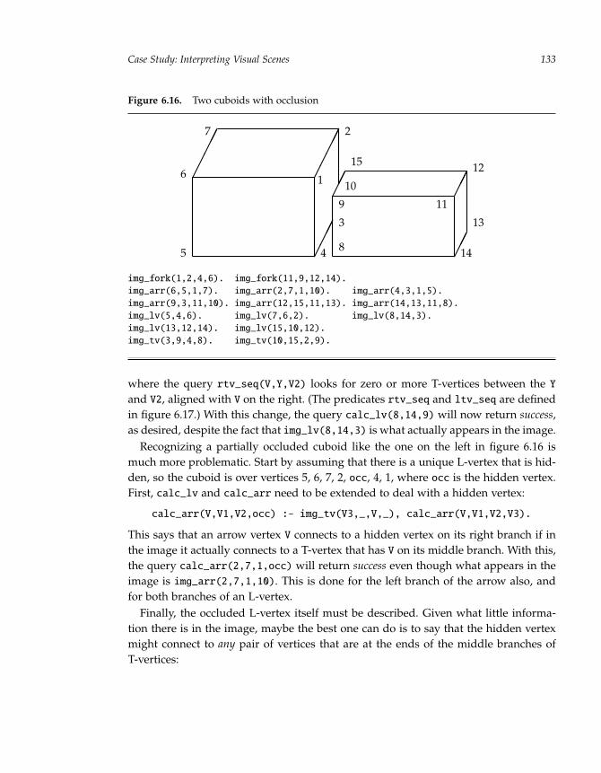
‘‘run’’ --- 2011/9/8 --- 18:05 --- page 133 --- #156�

�

�

�

�

�

�

�


Figure 6.16. Two cuboids with occlusion

5

6

7

4

1

2

3

8

9

10

14

11

12

13

15

img_fork(1,2,4,6). img_fork(11,9,12,14).




img_lv(13,12,14). img_lv(15,10,12).

img_tv(3,9,4,8). img_tv(10,15,2,9).

where the query rtv_seq(V,Y,V2) looks for zero or more T-vertices between the Yand V2, aligned with V on the right. (The predicates rtv_seq and ltv_seq are definedin figure 6.17.) With this change, the query calc_lv(8,14,9) will now return success,as desired, despite the fact that img_lv(8,14,3) is what actually appears in the image.

Recognizing a partially occluded cuboid like the one on the left in figure 6.16 ismuch more problematic. Start by assuming that there is a unique L-vertex that is hid-den, so the cuboid is over vertices 5, 6, 7, 2, occ, 4, 1, where occ is the hidden vertex.First, calc_lv and calc_arr need to be extended to deal with a hidden vertex:

calc_arr(V,V1,V2,occ) :- img_tv(V3,_,V,_), calc_arr(V,V1,V2,V3).

This says that an arrow vertex V connects to a hidden vertex on its right branch if inthe image it actually connects to a T-vertex that has V on its middle branch. With this,the query calc_arr(2,7,1,occ) will return success even though what appears in theimage is img_arr(2,7,1,10). This is done for the left branch of the arrow also, andfor both branches of an L-vertex.

Finally, the occluded L-vertex itself must be described. Given what little informa-tion there is in the image, maybe the best one can do is to say that the hidden vertexmight connect to any pair of vertices that are at the ends of the middle branches ofT-vertices:

“run” — 2011/9/8 — 18:05 — page 134 — #157�

�

�

�

�

�

�

�

Chapter 6134

Figure 6.17. Finding vertices with occlusion occlusion.pl

calc_arr(V,V1,V2,V3) :-

img_arr(V,X,V2,Y), ltv_seq(V,X,V1), rtv_seq(V,Y,V3).

calc_arr(V,V1,V2,occ) :- img_tv(V3,_,V,_), calc_arr(V,V1,V2,V3).

calc_arr(V,occ,V2,V3) :- img_tv(V1,_,V,_), calc_arr(V,V1,V2,V3).

calc_lv(V,V1,V2) :-

img_lv(V,X,Y), ltv_seq(V,X,V1), rtv_seq(V,Y,V2).

calc_lv(V,V1,occ) :- img_tv(V2,_,V,_), calc_lv(V,V1,V2).

calc_lv(V,occ,V2) :- img_tv(V1,_,V,_), calc_lv(V,V1,V2).

calc_lv(occ,V1,V2) :- img_tv(_,_,V1,_), img_tv(_,_,V2,_), \+ V1=V2.

% ltv_seq(V,X,Y): V X ... Y via T-vertices left to right

ltv_seq(_,X,X).

ltv_seq(V,X,Y) :- img_tv(X,V,_,Z), ltv_seq(X,Z,Y).

% rtv_seq(V,X,Y): V X ... Y via T-vertices right to left

rtv_seq(_,X,X).

rtv_seq(V,X,Y) :- img_tv(X,Z,_,V), rtv_seq(X,Z,Y).

calc_lv(occ,V1,V2) :-

img_tv(_,_,V1,_), img_tv(_,_,V2,_), \+ V1=V2.

This is a very permissive rule, as there could be many T-vertices in an image. Butit does allow calc_lv(occ,2,4) to return success for this image, as desired. Andwith all the other constraints in place for a cuboid, it will be sufficient. (If there wereadditional image properties, one could be more selective.)

With all the pieces together for calc_arr and calc_lv, the occlusion program isshown in figure 6.17. This will also handle the nonoccluded vertices as a special case.If it is combined with the earlier definitions of cuboid and calc_fork from figure 6.15and run on the image in figure 6.16, the result is

?- cuboid(A,B,C,D,E,F,G).

A = 6, B = 7, C = 2, D = occ, E = 4, F = 5, G = 1 ;

A = 9, B = 15, C = 12, D = 13, E = 14, F = 8, G = 11 ;

A = 12, B = 13, C = 14, D = 8, E = 9, F = 15, G = 11 ;

A = 14, B = 8, C = 9, D = 15, E = 12, F = 13, G = 11 ;

A = 2, B = occ, C = 4, D = 5, E = 6, F = 7, G = 1 ;

A = 4, B = 5, C = 6, D = 7, E = 2, F = occ, G = 1 ;

No

So the final program is able to tease apart the two objects and find all three viewsof the occluding cuboid and all three views of the occluded cuboid.

“run” — 2011/9/8 — 18:05 — page 135 — #158�

�

�

�

�

�

�

�


Want to read more?

This chapter was about interpreting visual scenes; it showed how thinking played afundamental role in that process. (The picture in Figure 6.2 is taken from [35].) Theaerial sketch map interpretation of section 6.2 was inspired by the work of Reiterand Mackworth [34], and the object recognition task of section 6.4 has appearedin many guises and is the subject of a textbook by Grimson [32]. Other studies ofknowledge-based vision include the early work of Badler [29] and Tsotsos [36], con-cerning motion in visual scenes. Another related area is reasoning about space andhow shapes occupy it (see, for example, [30]). For a retrospective on the problem ofvisual interpretation as a whole, including some of the challenges faced by researchersin the field, see [31]. From a more artistic point of view, the idea of impossible objectsand visual ambiguity is exploited to great effect in the work of M. C. Escher (see, forexample, his Relativity).

However, much of what happens when we view the world around us appears totake place without any knowledge of the world, and therefore (by the account here)without any thinking. For example, we do not have to know what we are lookingat to spot something yellow in a large field of red. Pylyshyn [33] has written a bookexplaining how this part of the visual process is very different from thinking. Thesubarea of AI called computer vision is currently dominated by research on “earlyvision” of this sort.

The polyhedral scene labeling considered in section 6.3 is an interesting intermedi-ate case. It comes out of the work of Waltz [37] in the 1970s and was one of the firsttasks formulated as a constraint satisfaction problem. However, it is not necessary toknow very much about the world to perform this task. There are vertex types and linelabels but no open-ended class of objects like vehicles or houses or banquet tables. Forthis reason, Pylyshyn prefers to categorize this task as not depending on thinking atall, but rather as embodying what he calls “natural constraints.”

If you reflect on what it actually feels like to look at visual scenes, you might betempted to conclude that the thinking is really quite unlike constraint satisfaction. Itseems like visual interpretations come to you without any mental effort—nothing atall like solving a Sudoku puzzle, for instance. Part of this feeling is due to the fact thatyour eyes are able to quickly dart back and forth over a scene, too quickly to registerhow you are using what you know. To get a better sense of how a visual interpretationis assembled, imagine that you cannot move your eyes in this way. Simulate this bycutting a small hole in a sheet of paper, looking at an image like figure 6.2 throughthe hole only, and then slowly moving the paper to take in the entire scene.

“run” — 2011/9/8 — 18:05 — page 136 — #159�

�

�

�

�

�

�

�

“run” — 2011/9/8 — 18:05 — page 137 — #160�

�

�

�

�

�

�

�

7 Lists in Prolog

Before moving on to consider bigger and better varieties of thinking, this chapterbrings the programming skills learned so far up to the next level.

The Prolog symbols in previous chapters were single atomic units: constants, vari-ables, numbers. This chapter considers larger symbolic structures called lists, and somepredicates that assemble them and take them apart.

Lists are essential to the sorts of thinking studied in the chapters to follow.Chapter 8, for example, deals with thinking about sentences and phrases of English,and these end up being lists of words. Chapter 9 surveys thinking about plans toachieve goals, and these end up being lists of actions to perform.

The first section of this chapter introduces lists and the two notations in Prolog thatare used for them. Section 2 considers how to write the clauses for predicates thattake lists as arguments, allowing properties over groups of objects to be expressedvery succinctly. Section 3 explains how to use two very useful built-in list predicates,member and append, and reformulates in a clear and concise way the blocks-worldprogram from section 4.2.

7.1 Lists

A problem that comes up again and again in Prolog is writing clauses for predicatesthat are very similar except for the number of arguments they take. Consider, forexample, the predicates used in chapter 5 to ensure that individuals in a group wereall distinct:

uniq_person3(X,Y,Z) :- ... % For three people

uniq_person5(X,Y,Z,U,V) :- ... % For five people

The uniq_digits predicate in figure 5.8 handles eight digits and has (8 × 7)/2 = 28inequalities in it. If there were eighteen people, one would need a predicate like this:

uniq_person18(A,B,C,D,E,F,G,H,I,J,K,L,M,N,O,P,Q,R) :- ...

“run” — 2011/9/8 — 18:05 — page 138 — #161�

�

�

�

�

�

�

�

Chapter 7138

where the body would contain (18 × 17)/2 = 153 inequalities. It would clearly bemuch better to be able to write just one predicate, like this:

uniq_people(L) :- ... % For any number of people

This predicate would have to work for any collection L of people, no matter how bigor small. Prolog provides such a collection, and it is called a list.

A Prolog list is a sequence of objects that are called its elements. Here are someexamples:

[anna,karenina]

A two-element list whose first element is the constant anna and whose secondelement is the constant karenina.

[john,paul,george,ringo,zeppo]

A five-element list.

[1,2,3,3,2,1]

Lists may have repeated elements.

[]

A list with no elements: the empty list.

Lists may contain other lists as elements:

[[john,23],[mary,14],[hello]]

A list whose three elements are also lists.

[8,john,[’199y’,john]]

Another three-element list.

[[]]

A one-element list whose single element is the empty list.

Note that a one-element list is different from the element itself:

[anna] is different from anna;

[[]] is different from [].

The first element of a nonempty list is called the head of the list. The list that is formedby removing that first element (and the comma that follows it, if there is one) is calledthe tail of the list. Here are some examples:

[a,b,c,d] has head a and tail [b,c,d];

[[a],b,[c]] has head [a] and tail [b,[c]];

[a,[b,c]] has head a and tail [[b,c]];

“run” — 2011/9/8 — 18:05 — page 139 — #162�

�

�

�

�

�

�

�

Lists in Prolog 139

[[a,b]] has head [a,b] and tail [];

[] has neither head nor tail.

The head of a nonempty list can be anything, but the tail is always a list. This turnsout to be a very convenient property when it comes to recursion.

7.1.1 Lists as Prolog terms

The review of the Prolog language in figure 3.10 can now be extended to say thata Prolog term is a constant, variable, number, or list. Prolog provides two ways ofwriting lists as terms:

1. A left square parenthesis, followed by a sequence of terms separated by commas,and terminated by a right square parenthesis, for example,

[1,-4,[a,X,’b 2’],joe]

2. A left square parenthesis, followed by a nonempty sequence of terms separatedby commas, followed by a vertical bar |, followed by a term denoting a list, andterminated by a right square parenthesis. For example, the list [1,X,3] can bewritten as

[1|[X,3]] or[1,X|[3]] or[1,X,3|[]].

While the first notation focuses on the elements of a list, the second notation focuseson the head and tail of a list. The list [X|Y] is the list whose head is X and whose tailis Y; the list [X,Y|Z] is the list whose head is X and whose tail is the list whose headis Y and whose tail is Z. So, for example, the list [1|[X,3]] is the list whose head is 1and whose tail is [X,3], which is just another way of describing the list [1,X,3].

7.1.2 Unification with lists

Much of the power of lists in Prolog has to do with the fact that variables can appearwithin a list term. But this also brings up concern about which pairs of lists unify (asneeded for back-chaining). The basic rule is this:

Two lists without variables are considered to unify when they are identical,element for element.

Two lists with distinct variables are considered to unify when the variables canbe given values that make the two lists identical, element for element.

“run” — 2011/9/8 — 18:05 — page 140 — #163�

�

�

�

�

�

�

�

Chapter 7140

Here are some examples of pairs of lists that do unify:

[] and []

[a,b,c] and [a,b,c]

[X] and [a] with X=a

[a,b,X] and [Y,b,Y] with X=a, Y=a

[X,X] and [[Y,a,c],[b,a,c]] with X=[b,a,c], Y=b

[[X]] and [Y] with X=_G237, Y=[_G237]

[a,b,c] and [a|[b,c]]

[a,b,c] and [a|[b|[c]]]

[X|Y] and [a] with X=a, Y=[]

[a|[b,c]] and [a,X,Y] with X=b, Y=c

[a,b,c] and [X|Y] with X=a, Y=[b,c]

[X,Y|Y] and [a,[b,c],b,c] with X=a, Y=[b,c]

Lists will not unify if they have different numbers of elements or if at least onecorresponding element does not unify. Here are some nonunifying pairs:

[a] and [ ]

[a,b,c] and [a,a,c]

[] and [[]]

[X,Y] and [U,V,W]

[a,b,c] and [X,b,X]

[X|Y] and []

Here are some useful conclusions to draw from these examples:

X matches anything, including any list.[X] matches any list with exactly one element.[X|Y] matches any list with at least one element.[X,Y] matches any list with exactly two elements.

7.2 Writing programs that use lists

Programs that go through lists usually end up being recursive, since it may not beknown in advance how many elements are involved. Each list will have some numbern of elements. This is just like the recursion discussed in section 4.3, where a block that

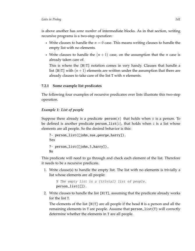
‘‘run’’ --- 2011/9/8 --- 18:05 --- page 141 --- #164�

�

�

�

�

�

�

�

Lists in Prolog 141

is above another has some number of intermediate blocks. As in that section, writingrecursive programs is a two-step operation:

Write clauses to handle the n = 0 case. This means writing clauses to handle theempty list with no elements.

Write clauses to handle the (n + 1) case, on the assumption that the n case isalready taken care of.

This is where the [H|T] notation comes in very handy. Clauses that handle alist [H|T] with (n + 1) elements are written under the assumption that there arealready clauses to take care of the list T with n elements.

7.2.1 Some example list predicates

The following four examples of recursive predicates over lists illustrate this two-stepoperation.

Example 1: List of people

Suppose there already is a predicate person(x) that holds when x is a person. Tobe defined is another predicate person_list(z), that holds when z is a list whoseelements are all people. So the desired behavior is this:

?- person_list([john,sue,george,harry]).

Yes

?- person_list([john,5,harry]).

No

This predicate will need to go through and check each element of the list. Thereforeit needs to be a recursive predicate.

1. Write clause(s) to handle the empty list. The list with no elements is trivially alist whose elements are all people:

% The empty list is a (trivial) list of people.

person_list([]).

2. Write clauses to handle the list [H|T], assuming that the predicate already worksfor the list T.

The elements of the list [H|T] are all people if the head H is a person and all theremaining elements in T are people. Assume that person_list(T) will correctlydetermine whether the elements in T are all people.

“run” — 2011/9/8 — 18:05 — page 142 — #165�

�

�

�

�

�

�

�

Chapter 7142

Figure 7.1. A trace of a list predicate

?- person_list([john,sue]).

Call: (7) person_list([john, sue])

Call: (8) person(john)

Exit: (8) person(john)

Call: (8) person_list([sue])

Call: (9) person(sue)

Exit: (9) person(sue)

Call: (9) person_list([]) % This is where the first

Exit: (9) person_list([]) % clause is used.

Exit: (8) person_list([sue])

Exit: (7) person_list([john, sue])

% If H is a person and T is a list of people,

% then [H|T] is also a list of people.

person_list([H|T]) :- person(H), person_list(T).

These two clauses complete the definition. A trace of a query appears in figure 7.1.Here is how unification works with the two clauses during back-chaining:

1. [john,sue] does not unify with [] in the first clause, but it does unify with [H|T]in the second clause for H=john and T=[sue].

2. [sue] does not unify with [], but it does unify with [H|T] for H=sue and T=[].

3. [] unifies with [], and the predicate succeeds immediately.

Note how the two notations for lists work together.

Example 2: Membership in a list

Define a predicate elem that will determine whether something is an element of a list.This is the desired behavior:

?- elem(b,[a,b,c,d]).

Yes

?- elem(f,[a,b,c,d]).

No

Prolog systems provide a predefined predicate, member, with exactly this behavior,but the following defines a version as a recursive predicate:

1. Write clauses for the empty list. There is nothing to write here since the queryelem(X,[]) should always fail.

“run” — 2011/9/8 — 18:05 — page 143 — #166�

�

�

�

�

�

�

�

Lists in Prolog 143

2. Write clauses to handle the list [H|T], assuming the list T is already taken care of.The query elem(X,[H|T]) should succeed if X is equal to H, or if X is an elementof list T. So two clauses are needed:

% X is an element of any list whose head is X.

elem(X,[X|_]).

% If X is an element of a list L,

% then it is an element of any list whose tail is L.

elem(X,[_|L]) :- elem(X,L).

Note the use of the anonymous variable. In the first clause, the query succeeds nomatter what the tail is; in the second clause, the query succeeds no matter what thehead is.

We can follow the behavior in a trace:

?- elem(c,[a,b,c,d]).

Call: (7) elem(c,[a,b,c,d])

Call: (8) elem(c,[b,c,d])

Call: (9) elem(c,[c,d]) % Here the first clause is used and

Exit: (9) elem(c,[c,d]) % succeeds immediately.

Exit: (8) elem(c,[b,c,d])

Exit: (7) elem(c,[a,b,c,d])

Example 3: List of unique people

The member predicate (or the elem predicate just defined) can be used to write theclauses for a predicate uniq_people(z) that holds when z is any list of people that areall distinct, as needed for many constraint satisfaction problems. As before, assumethat a predicate person is already defined. The uniq_people predicate will once againbe recursive:

1. The empty list [] is a (trivial) list of unique people.

2. For the list [P|L], if P is a person, L is a list of unique people, and in addition, Pis not an element of L, then [P|L] is also a list of unique people.

This gives a definition of the predicate with the following two clauses:

uniq_people([]).

uniq_people([P|L]) :- uniq_people(L), person(P), \+ member(P,L).

This recursive predicate will work properly for lists of any size. Note how succinctand elegant this definition is compared to the long sequences of inequalities writtenin chapter 5 for each constraint satisfaction problem.

“run” — 2011/9/8 — 18:05 — page 144 — #167�

�

�

�

�

�

�

�

Chapter 7144

∗ Example 4: Joining two lists

Here is a more advanced example. Define a predicate join that concatenates two lists:

?- join([a,b,c,d],[e,f,g],L).

L=[a,b,c,d,e,f,g]

Yes

?- join([],[a,b,c,d],L).

L=[a,b,c,d]

Yes

Prolog systems provide a predefined predicate, append, with exactly this behavior,but again a version is defined here as a recursive predicate.

The predicate join needs to determine what the third argument (the answer)should be for any two lists. The first list can be empty or nonempty, and the sec-ond list can also be empty or nonempty. However, it turns out that it is sufficient todo recursion on the first argument only:

1. Write clauses to handle the case where the first argument is [] and the secondargument is any list L;

2. Write clauses to handle the case where the first argument is [H|T] and the sec-ond argument is any list L (assuming that join already works when the firstargument is T and the second argument is L).

This leads to the following two clauses:

% Joining [] and any list L produces L itself.

join([],L,L).

% If joining T and L produces the list Z,

% then joining [H|T] and L produces the list [H|Z].

join([H|T],L,[H|Z]) :- join(T,L,Z).

The head of the second clause is quite complex. Much of the work of join is done byunification with this head.

A trace is shown in figure 7.2. As the query succeeds at each level, new elementsare added to the third argument, building the final concatenated list. Here is how theunification works:

1. The top-level query is join([a,b,c,d],[e,f],R).

2. This does not unify with join([],L,L), but it unifies with join([H|T],L,[H|Z])for the following values: H=a, T=[b,c,d], L=[e,f], and R=[a|Z].

“run” — 2011/9/8 — 18:05 — page 145 — #168�

�

�

�

�

�

�

�

Lists in Prolog 145

Figure 7.2. Another trace of a list predicate

?- join([a,b,c,d],[e,f],R).

Call: (3) join([a,b,c,d],[e,f],_G306)

Call: (4) join([b,c,d],[e,f],_G378)

Call: (5) join([c,d],[e,f],_G381)

Call: (6) join([d],[e,f],_G384)

Call: (7) join([],[e,f],_G387) % Now the first clause is used.

Exit: (7) join([],[e,f],[e,f]) % It succeeds immediately.

Exit: (6) join([d],[e,f],[d,e,f])

Exit: (5) join([c,d],[e,f],[c,d,e,f])

Exit: (4) join([b,c,d],[e,f],[b,c,d,e,f])

Exit: (3) join([a,b,c,d],[e,f],[a,b,c,d,e,f])

R = [a,b,c,d,e,f]

Yes

3. The new query is then join(T,L,Z), that is, join([b,c,d],[e,f],Z).

4. This subquery does not unify with the head of the first clause, but it does unifywith the head of the second clause.

5. Eventually, this subquery succeeds with Z=[b,c,d,e,f].

6. Then the top-level query succeeds with R=[a|Z], that is, R=[a,b,c,d,e,f].

7.3 Using the member and append predicates

From now on, the built-in Prolog predicates member and append (which behave likeelem and join) are used in the examples. One very useful application of member is togenerate the elements of a list:

?- member(X,[a,b,c]).

X = a ;

X = b ;

X = c ;

No

This means that queries (or bodies of clauses) can be written that go through theelements of a list looking for one that satisfies some condition:

. . . member(X,L), p(X), . . .

“run” — 2011/9/8 — 18:05 — page 146 — #169�

�

�

�

�

�

�

�

Chapter 7146

If L is a nonempty list, and the variable X is not instantiated, the member(X,L) querywill succeed, with X getting the head of the list as its value. If the query p(X) thenfails, the program will backtrack, and X will be assigned to the next element of thelist, and so on, until an element of L is found for which p(X) succeeds. Here is anexample of this generate-and-test in a query:

?- member(N,[1,2,3,-3,5,-5,7]), N < 0.

N = -3 ; % The first element that is < 0

N = -5 ; % The second element that is < 0

No

However, when using list predicates to generate values in this way, one must becareful not to generate an infinite set of candidates. Consider the following:

?- member(3,L). % What list has 3 as an element?

L = [3|_G214] ; % Any list whose first element is 3,

L = [_G213, 3|_G217] ; % any list whose second element is 3,

L = [_G213, _G216, 3|_G220] % and so on.

Yes

?- member(3,L), 1=2.

ERROR: Out of global stack % This query causes an error.

In the second query, each time the subquery 1=2, fails, the program backtracks to tryto find a new value for L. Since there will always be another value to consider (that is,a bigger list), the process runs until L gets so large that it causes an error. This caveataside, variables can be used in either argument of the member predicate:

?- member(a,[X,b,Y]).

X = a, Y = _G163 ;

X = _G157, Y = a ;

No

?- L=[a,X,b], member(3,L).

L = [a, 3, b], X = 3 ;

No

?- L=[X,b,Y], member(a,L), member(X,[b,c]).

L = [b, b, a], X = b, Y = a ;

L = [c, b, a], X = c, Y = a ;

No

So unlike numbers, variables that are not instantiated can be used within lists. Prologfinds their values when it needs to.

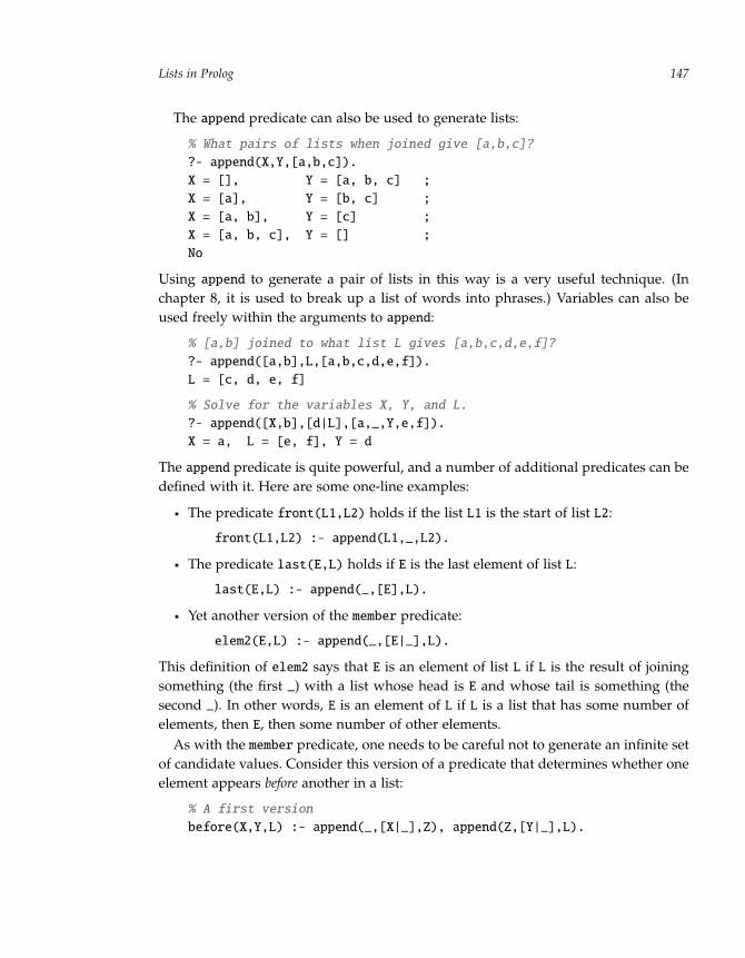
“run” — 2011/9/8 — 18:05 — page 147 — #170�

�

�

�

�

�

�

�

Lists in Prolog 147

The append predicate can also be used to generate lists:

% What pairs of lists when joined give [a,b,c]?

?- append(X,Y,[a,b,c]).

X = [], Y = [a, b, c] ;

X = [a], Y = [b, c] ;

X = [a, b], Y = [c] ;

X = [a, b, c], Y = [] ;

No

Using append to generate a pair of lists in this way is a very useful technique. (Inchapter 8, it is used to break up a list of words into phrases.) Variables can also beused freely within the arguments to append:

% [a,b] joined to what list L gives [a,b,c,d,e,f]?

?- append([a,b],L,[a,b,c,d,e,f]).

L = [c, d, e, f]

% Solve for the variables X, Y, and L.

?- append([X,b],[d|L],[a,_,Y,e,f]).

X = a, L = [e, f], Y = d

The append predicate is quite powerful, and a number of additional predicates can bedefined with it. Here are some one-line examples:

The predicate front(L1,L2) holds if the list L1 is the start of list L2:

front(L1,L2) :- append(L1,_,L2).

The predicate last(E,L) holds if E is the last element of list L:

last(E,L) :- append(_,[E],L).

Yet another version of the member predicate:

elem2(E,L) :- append(_,[E|_],L).

This definition of elem2 says that E is an element of list L if L is the result of joiningsomething (the first _) with a list whose head is E and whose tail is something (thesecond _). In other words, E is an element of L if L is a list that has some number ofelements, then E, then some number of other elements.

As with the member predicate, one needs to be careful not to generate an infinite setof candidate values. Consider this version of a predicate that determines whether oneelement appears before another in a list:

% A first version

before(X,Y,L) :- append(_,[X|_],Z), append(Z,[Y|_],L).

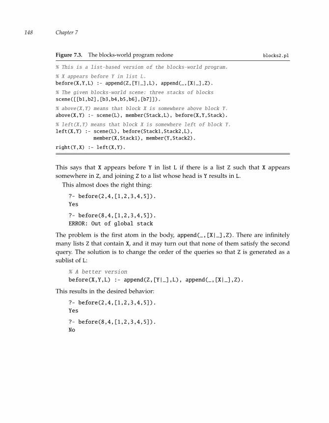
“run” — 2011/9/8 — 18:05 — page 148 — #171�

�

�

�

�

�

�

�

Chapter 7148

Figure 7.3. The blocks-world program redone blocks2.pl

% This is a list-based version of the blocks-world program.

% X appears before Y in list L.

before(X,Y,L) :- append(Z,[Y|_],L), append(_,[X|_],Z).

% The given blocks-world scene: three stacks of blocks

scene([[b1,b2],[b3,b4,b5,b6],[b7]]).

% above(X,Y) means that block X is somewhere above block Y.

above(X,Y) :- scene(L), member(Stack,L), before(X,Y,Stack).

% left(X,Y) means that block X is somewhere left of block Y.

left(X,Y) :- scene(L), before(Stack1,Stack2,L),

member(X,Stack1), member(Y,Stack2).

right(Y,X) :- left(X,Y).

This says that X appears before Y in list L if there is a list Z such that X appearssomewhere in Z, and joining Z to a list whose head is Y results in L.

This almost does the right thing:

?- before(2,4,[1,2,3,4,5]).

Yes

?- before(8,4,[1,2,3,4,5]).

ERROR: Out of global stack

The problem is the first atom in the body, append(_,[X|_],Z). There are infinitelymany lists Z that contain X, and it may turn out that none of them satisfy the secondquery. The solution is to change the order of the queries so that Z is generated as asublist of L:

% A better version

before(X,Y,L) :- append(Z,[Y|_],L), append(_,[X|_],Z).

This results in the desired behavior:

?- before(2,4,[1,2,3,4,5]).

Yes

?- before(8,4,[1,2,3,4,5]).

No

“run” — 2011/9/8 — 18:05 — page 149 — #172�

�

�

�

�

�

�

�

Lists in Prolog 149

Figure 7.4. Using the list version of the blocks world program

?- left(b1,b7).

Call: (7) left(b1, b7)

Call: (8) scene(_L205) % Get the scene.

Exit: (8) scene([[b1, b2], [b3, b4, b5, b6], [b7]])

% Generate a first pair of stacks.

Call: (8) before(_L206, _L207, ...)

Exit: (8) before([b1, b2], [b3, b4, b5, b6],...)

Call: (8) member(b1, [b1, b2]) % Test if X is in the first.

Exit: (8) member(b1, [b1, b2]) % YES

Call: (8) member(b7, [b3, b4, b5, b6]) % Test if Y is in the second.

Fail: (8) member(b7, [b3, b4, b5, b6]) % NO

Redo: (8) member(b1, [b1, b2])

Fail: (8) member(b1, [b1, b2])

% Generate another pair of stacks.

Redo: (8) before(_L206, _L207, ...)

Exit: (8) before([b1, b2], [b7], ...)

Call: (8) member(b1, [b1, b2]) % Test if X is in the first.

Exit: (8) member(b1, [b1, b2]) % YES

Call: (8) member(b7, [b7]) % Test if Y is in the second.

Exit: (8) member(b7, [b7]) % YES

Exit: (7) left(b1, b7) % The second pair works.

Yes

7.3.1 The blocks world revisited

The predicates member and append can be used to define a much more succinct versionof the blocks-world program (see section 4.2).

Here is the idea. An entire blocks-world scene can be represented by a left-to-rightlist of stacks, where a stack is represented by a top-to-bottom list of blocks. So thescene depicted in figure 4.1 is represented by the following list:

[[b1,b2],[b3,b4,b5,b6],[b7]]

The predicates above and left can then be defined using the before predicate:

A block X is above a block Y in the scene if there is a stack in the scene where Xappears before Y in the stack.

A block X is somewhere to the left of a block Y if there is a stack in the scene thatcontains X that is before a stack in the scene that contains Y.

The full blocks-world program is shown in figure 7.3. A trace of the left predicate isshown in figure 7.4.

“run” — 2011/9/8 — 18:05 — page 150 — #173�

�

�

�

�

�

�

�

Chapter 7150

Want to read more?

This chapter considered programming in Prolog, concentrating on programs that dealwith lists. This type of list processing, which involves dealing with collections ofsymbols as single larger units, has a long history. The first truly symbolic (that is, non-numerical) programming language, called IPL, was also the first to provide explicitfacilities for dealing with lists. A more influential and still quite popular program-ming language of this sort is LISP [38] and its direct descendant, Scheme [53]. BothLISP and Scheme take list processing as their central focus.

A few simple examples of list-processing predicates were reviewed in this chapter.The blocks-world program was rewritten using lists, and many other programs inprevious chapters could be redone more clearly using lists. It takes time and practiceto master this type of programming, however. A typical second-year or third-yearundergraduate computer science course might involve writing predicates that aresimilar to append but perhaps more complex (for example, a predicate that returnsevery second element of a list, or a predicate that sorts a list of numbers into ascendingorder). Any programming textbook on Prolog (such as those mentioned at the end ofchapter 4) will cover writing predicates like these.

It turns out, however, there are even more advanced list-processing techniques thatcan be employed in Prolog but that do not fit well in other programming languages.In particular, the fact that an uninstantiated variable can be an element of a list allowscertain operations to be performed very elegantly in Prolog, by building a list butleaving parts of it unspecified at first. These techniques and many more are coveredin the more advanced Prolog textbooks such as [39].

Exercises

1. The text defined a predicate elem(x, y) that held when x was an element of thelist y. Consider the following variant:

elem3(X,[X]).

elem3(X,[_|L]) :- elem3(X,L).

Give an example of an x and a y such that elem(x, y) holds but where elem3(x, y)does not hold. Describe in English when the predicate elem3(x, y) holds ingeneral.

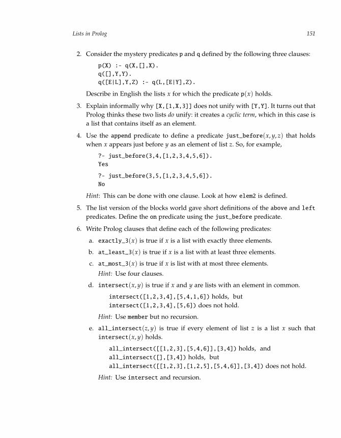
“run” — 2011/9/8 — 18:05 — page 151 — #174�

�

�

�

�

�

�

�

Lists in Prolog 151

2. Consider the mystery predicates p and q defined by the following three clauses:

p(X) :- q(X,[],X).

q([],Y,Y).

q([E|L],Y,Z) :- q(L,[E|Y],Z).

Describe in English the lists x for which the predicate p(x) holds.

3. Explain informally why [X,[1,X,3]] does not unify with [Y,Y]. It turns out thatProlog thinks these two lists do unify: it creates a cyclic term, which in this case isa list that contains itself as an element.

4. Use the append predicate to define a predicate just_before(x, y, z) that holdswhen x appears just before y as an element of list z. So, for example,

?- just_before(3,4,[1,2,3,4,5,6]).

Yes

?- just_before(3,5,[1,2,3,4,5,6]).

No

Hint: This can be done with one clause. Look at how elem2 is defined.

5. The list version of the blocks world gave short definitions of the above and leftpredicates. Define the on predicate using the just_before predicate.

6. Write Prolog clauses that define each of the following predicates:

a. exactly_3(x) is true if x is a list with exactly three elements.

b. at_least_3(x) is true if x is a list with at least three elements.

c. at_most_3(x) is true if x is list with at most three elements.

Hint: Use four clauses.

d. intersect(x, y) is true if x and y are lists with an element in common.

intersect([1,2,3,4],[5,4,1,6]) holds, butintersect([1,2,3,4],[5,6]) does not hold.

Hint: Use member but no recursion.

e. all_intersect(z, y) is true if every element of list z is a list x such thatintersect(x, y) holds.

all_intersect([[1,2,3],[5,4,6]],[3,4]) holds, andall_intersect([],[3,4]) holds, butall_intersect([[1,2,3],[1,2,5],[5,4,6]],[3,4]) does not hold.

Hint: Use intersect and recursion.

“run” — 2011/9/8 — 18:05 — page 152 — #175�

�

�

�

�

�

�

�

“run” — 2011/9/8 — 18:05 — page 153 — #176�

�

�

�

�

�

�

�

8 Case Study: Understanding Natural Language

This chapter turns attention to the sort of thinking required to make sense of expres-sions in a natural language, that is, a language like English or Italian or Swahili that isspoken naturally by people.

When it comes to tasks that require thinking, understanding language holds aposition of honor. One of the features that distinguishes humans from all other livingcreatures is our ability to communicate using a system as rich as a natural language.And to deal with this richness, we need to be able to think. A speaker can say wordslike “the American President during the Civil War” and expect that under normalcircumstances a hearer will use what she knows to make a connection with AbrahamLincoln. This need for thinking was displayed in a very simple but pure form inchapter 1 in resolving the pronoun it in the trophy-suitcase sentences.

But the connection between thinking and language goes even deeper. It is not justthat thinking supports our ability to use language; the converse is also true: languagefeeds our thinking. As emphasized throughout, thinking is using what we know, andmuch of what we know is due to language. We find out about the world and thepeople around us to a large extent not from personal experience but by being told:people talk to us, we attend lectures, we listen to weather reports and to the dialoguein movies, and we read: text messages, recipes, sport scores, mystery novels, andso on. What we know and use in our thinking is a staggering amount of language-mediated material. We pass on to our descendants much more of this information inwritten form than all of the genetic information in our DNA. Given this dependenceon language, it is not surprising that thinking often feels like using a language, talkingto ourselves in some sort of inner voice.

This chapter only scratches the surface of the truly remarkable story of how lan-guage can both depend on thinking and provide the raw material for it. Section 1explains how language is usually studied in terms of syntax and semantics. Section 2focuses on the noun phrases of English and how they can be used to refer to knownindividuals and objects. Section 3 examines how these noun phrases can be put towork in answering yes/no questions written in English and in adding to what isknown using English declarative sentences. (To do so, a new feature of Prolog is

“run” — 2011/9/8 — 18:05 — page 154 — #177�

�

�

�

�

�

�

�

Chapter 8154

introduced: dynamic predicates.) Section 4 briefly discusses how the utility of nounphrases actually is even more extensive.

8.1 Analyzing the syntax of a language

Although the expressions of a written language are nothing more than sequencesof words and punctuation, what those sequences are and how they can be used isphenomenally complex. The study of natural language in general is called linguistics,and it analyzes language at a variety of levels:

Morphology: What are the roots of words, the prefixes and suffixes?

ran = run + PASTchildren = child + PLURAL

Syntax: How do the words group together?

Mary kicked the boy in the knee.

Mary kicked the boy in the first row.

Semantics: What do the words mean?

The astronomer spotted a star.

The astronomer married a star.

The trophy would not fit into the brown suitcase

because it was too small.

because it was too big.

Pragmatics: What are the words being used for?

Can you juggle?

Can you pass the salt?

(There are additional levels for spoken language, such as phonology and prosod-ics.) This chapter concentrates mainly on the syntax of written English, with someexcursions into semantics.

A syntactic analysis of a language looks at how words group together into phrases,sentences, and even larger units like paragraphs and stories. For example, considerthe following phrase:

the boy in the park with the red bench

Clearly the intention is to group words in this phrase as follows:

“run” — 2011/9/8 — 18:05 — page 155 — #178�

�

�

�

�

�

�

�

Case Study: Understanding Natural Language 155

(the boy in (the park with (the red bench)))

Now, consider the following instead:

the boy in the park with the gray sweater

In this case, the words would be grouped differently, perhaps as follows:

(the boy in (the park) with (the gray sweater))

The main point of these groupings is that in the first case, the phrase with the red

bench is understood as being connected to the park; in the second case, with the gray

sweater is understood as being connected to the boy. It might not be obvious on firstreading what should be grouped with what. For example,

The cat the dog the boy next door owns chases sleeps all day.

may only be resolved with some difficulty to a grouping like the following:

(The cat (the dog (the boy next door owns) chases) sleeps all day).

Knowing how the words in a phrase or sentence should be grouped together is notthe same thing as understanding what they mean (which is the subject of semantics).In particular, there can be sentences of English that are syntactically well formed butdo not mean anything. Here is a famous example (due to Noam Chomsky):

Colorless green ideas sleep furiously.

The pattern and the grouping of these words are familiar even if the sentence isodd semantically. Similarly, there can be meaningful groups of words that are oddsyntactically:

Accident car passenger hospital.

Even though this is not a well-formed sentence of English, one can still extract at leastpart of its meaning.

8.1.1 Lexicon

The starting point for the syntactic analysis of a language is a lexicon. This specifiesthe word categories of the language and the vocabulary in each category:

Articles: a, the

Adjectives: fat, rich, happy, oldest, orange, . . .

Proper nouns: Mary, John, Toronto, Great Britain, . . .

Common nouns: boy, sweater, park, milk, justice, . . .

“run” — 2011/9/8 — 18:05 — page 156 — #179�

�

�

�

�

�

�

�

Chapter 8156

Transitive verbs: kick, love, throw, make, . . .

Intransitive verbs: walk, sleep, die, listen, . . .

Copula verbs: be, seem, . . .

Prepositions: in, on, from, beside, . . .

Others (pronouns, adverbs, interjections, . . . )

Note that words can appear in more than one category. For example, the word run inEnglish is both a noun and a verb; the word fat is both a noun and an adjective.

8.1.2 Grammar

A grammar of a language is a specification of how the various types of words canbe grouped in the language. These word groups are called the syntactic categories. Adistinction is made between the following:

Lexical or terminal categories, like an article or a transitive verb. These will bewritten in lowercase.

Group or nonterminal categories, like a phrase or a sentence. These will be writtenin uppercase. (It is customary in linguistics to name the nonterminal categoriesof a language using short, cryptic abbreviations like NP for noun phrase.)

Usually grammars are specified by a collection of rules (similar to Prolog clauses)describing how each type of word group is formed from other word groups. Forpresent purposes, a grammar rule will have the following form:

category → category1 category2 . . . categoryn

where the category on the left must be nonterminal, and the categories on the right(if any) can be terminal or nonterminal. For example, the grammar rule

PP → preposition NP

says that in English a prepositional phrase (PP) can be made up of a prepositionfollowed by a noun phrase (NP).

Figure 8.1 shows a grammar for some declarative sentences of English. Starting atthe top, the rule says that a sentence S can be made from a noun phrase NP followed bya verb phrase VP. Note that this grammar does not include many features of English,such as pronouns or clauses. Note also that the grammar is recursive: the categoryMods (modifiers), for instance, is made up of zero or more of the PP category. Thisallows stacking the modifiers, as in the following noun phrase: the boy from France in

the library on the phone with the gray sweater.

“run” — 2011/9/8 — 18:05 — page 157 — #180�

�

�

�

�

�

�

�


Figure 8.1. A grammar for declarative sentences

S → NP VP

VP → copula_verb Mods

VP → transitive_verb NP Mods

VP → intransitive_verb Mods

Mods →Mods → PP Mods

PP → preposition NP

NP → proper_noun

NP → article NP2

NP2 → adjective NP2

NP2 → common_noun Mods

Figure 8.2. A sample parse tree

fat cat is onThe the mat.

NP

NP2article NP

NP2articleNP2adjective

Modsnoun Modsnoun

Mods

ModsPP

S

VP

copula

preposition

8.1.3 Parsing and ambiguity

The process of taking a sequence of words and determining how they are structuredby the rules of a grammar is called parsing. This is done by producing a parse tree,with the sequence of words at the leaves (usually at the bottom) and the desirednonterminal category at the root (usually at the top). A sample parse tree appears infigure 8.2. For any of the categories that appear in the tree, the leaves below them are

“run” — 2011/9/8 — 18:05 — page 158 — #181�

�

�

�

�

�

�

�

Chapter 8158

Figure 8.3. A sequence of words with two parse trees

This parse corresponds to thegrouping where with the hat

modifies boy.

This parse corresponds to the groupingwhere with the hat modifies park.

the words that make up that category. For example, the sequence on the mat is a PP,while the sequence is on the mat is a VP.

A grammar is said to be ambiguous if there is a sequence of words with two distinctparse trees. An example appears in figure 8.3. (The dashed lines indicate details thatare missing from the diagram.) According to the grammar, the noun phrase with the

hat can be attached as a modifier either to the NP2 that has the head noun boy (onthe left in the figure) or to the NP2 that has the head noun park (on the right). Itis only when semantics are taken into account that the ambiguity disappears. Priorknowledge provides the fact that boys, not parks, have hats. This is precisely the sortof thinking that is described, beginning in the next section.

8.2 Interpreting noun phrases

The goal in this section is to develop a Prolog program that does simple syntactic andsemantic processing of noun phrases written in English. This involves two things:

Parsing the noun phrases according to a given grammar

Determining what is being referred to by the noun phrases

“run” — 2011/9/8 — 18:05 — page 159 — #182�

�

�

�

�

�

�

�


To accomplish this, the knowledge base in Prolog has three distinct pieces:

1. A world model. These are clauses that represent what is known about the rel-evant world: what the objects are, who the people are, where they are located,what they are wearing, and so on. Nothing in the world model is intended to belanguage-specific.

2. A lexicon. These are clauses that describe the English words used in the nounphrases. They also link these words to their meanings in the predicates andconstants of the world model. Nothing in the lexicon depends on the grammar.

3. A parser/interpreter. These are clauses that define the grammar. They alsouse information provided by the lexicon and the world model to decide whatindividual is being referred to by the noun phrases.

8.2.1 Writing a world model

The world model is actually the easiest part of the Prolog program to write since itreally has nothing to do with English. All that is needed is a collection of clausesabout some world of interest, for example, the family world (figure 3.1) or the blocksworld (figure 4.2). To provide a wider range of individuals than those worlds contain,a new world is invented:

There are people, parks, trees, and hats to talk about. The people are either maleor female, the hats are either red or blue, and every person, tree, and hat is eithersmall or big. In addition, the people and trees are in the parks, and the hats areon the people. Finally, some of the people are beside others.

A Prolog program with these facts is shown in figure 8.4. This represents the back-ground knowledge that will be used in thinking about expressions in English. (Allthe clauses happen to be atomic, but this is not essential.)

8.2.2 Writing a lexicon

The lexicon needs to describe all the English words to be used and how they relateto the predicates and constants in the world model. The lexicon here is restricted toarticles, common nouns, adjectives, proper nouns, and prepositions using the follow-ing predicates: article, common_noun, adjective, proper_noun, and preposition.These predicates take one, two, or three arguments (the first of which will alwaysbe an English word). A sample lexicon of this form is shown in figure 8.5. Here is adescription:

“run” — 2011/9/8 — 18:05 — page 160 — #183�

�

�

�

�

�

�

�

Chapter 8160

Figure 8.4. A world of people, parks, trees, hats nldb.pl

person(john). person(george). person(mary). person(linda).

park(kew_beach). park(queens_park).

tree(tree01). tree(tree02). tree(tree03).

hat(hat01). hat(hat02). hat(hat03). hat(hat04).

sex(john,male). sex(george,male).

sex(mary,female). sex(linda,female).

color(hat01,red). color(hat02,blue).

color(hat03,red). color(hat04,blue).

in(john,kew_beach). in(george,kew_beach).

in(linda,queens_park). in(mary,queens_park).

in(tree01,queens_park). in(tree02,queens_park).

in(tree03,kew_beach).

beside(mary,linda). beside(linda,mary).

on(hat01,john). on(hat02,mary). on(hat03,linda). on(hat04,george).

size(john,small). size(george,big).

size(mary,small). size(linda,small).

size(hat01,small). size(hat02,small).

size(hat03,big). size(hat04,big).

size(tree01,big). size(tree02,small). size(tree03,small).

The predicate article(w) holds if the word w is an article.

The predicate common_noun(w, x) holds when the common noun w can be usedto refer to the object x in the world model. So, for example, this clause is in thelexicon:

common_noun(man,X) :- person(X), sex(X,male).

This says that if X is a person whose sex is male (in the world model), then X canbe what is referred to when using the common noun man. (This is intended torepresent what is known about the meaning of the word man.)

The predicate adjective(w, x) holds when the adjective w can be used todescribe the object x in the world model. This clause is in the lexicon:

adjective(red,X) :- color(X,red).

This says that if X has the color red (in the world model), then X can be what isreferred to when using the adjective red.

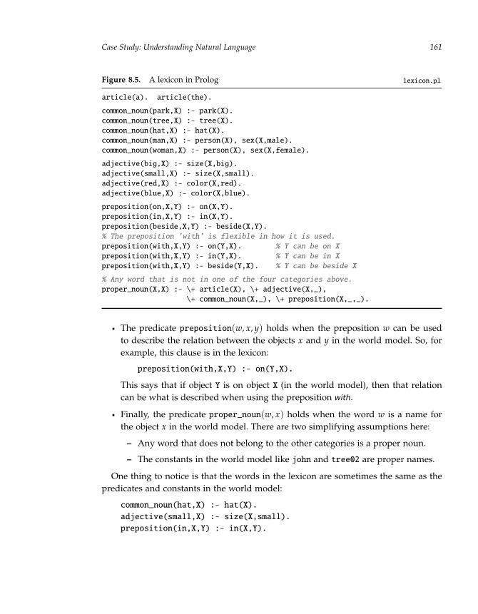
“run” — 2011/9/8 — 18:05 — page 161 — #184�

�

�

�

�

�

�

�


Figure 8.5. A lexicon in Prolog lexicon.pl

article(a). article(the).

common_noun(park,X) :- park(X).

common_noun(tree,X) :- tree(X).

common_noun(hat,X) :- hat(X).

common_noun(man,X) :- person(X), sex(X,male).

common_noun(woman,X) :- person(X), sex(X,female).

adjective(big,X) :- size(X,big).

adjective(small,X) :- size(X,small).

adjective(red,X) :- color(X,red).

adjective(blue,X) :- color(X,blue).

preposition(on,X,Y) :- on(X,Y).

preposition(in,X,Y) :- in(X,Y).

preposition(beside,X,Y) :- beside(X,Y).

% The preposition ’with’ is flexible in how it is used.

preposition(with,X,Y) :- on(Y,X). % Y can be on X

preposition(with,X,Y) :- in(Y,X). % Y can be in X

preposition(with,X,Y) :- beside(Y,X). % Y can be beside X

% Any word that is not in one of the four categories above.

proper_noun(X,X) :- \+ article(X), \+ adjective(X,_),

\+ common_noun(X,_), \+ preposition(X,_,_).

The predicate preposition(w, x, y) holds when the preposition w can be usedto describe the relation between the objects x and y in the world model. So, forexample, this clause is in the lexicon:

preposition(with,X,Y) :- on(Y,X).

This says that if object Y is on object X (in the world model), then that relationcan be what is described when using the preposition with.

Finally, the predicate proper_noun(w, x) holds when the word w is a name forthe object x in the world model. There are two simplifying assumptions here:

– Any word that does not belong to the other categories is a proper noun.

– The constants in the world model like john and tree02 are proper names.

One thing to notice is that the words in the lexicon are sometimes the same as thepredicates and constants in the world model:

common_noun(hat,X) :- hat(X).

adjective(small,X) :- size(X,small).

preposition(in,X,Y) :- in(X,Y).

“run” — 2011/9/8 — 18:05 — page 162 — #185�

�

�

�

�

�

�

�

Chapter 8162

But the lexicon and the world model have very different purposes:

The lexicon describes the words being used (like the English word hat).

The world model describes the facts in the world (like the concept of a hat).

The world model itself is intended to be language-neutral. Constants and predicateslike red and size are used in it, but just for convenience. As mentioned, Prologwould work the same on these if they were named property19 and concept42. Butthe lexicon is about the actual words, so there it is important to use constants thatcorrespond exactly to English (as the first argument to the lexicon predicates).

As a general rule, it is a good idea to distinguish between the world model and thelexicon for these two reasons:

Different words may be used for the same concept, as in the following:

– Synonyms

common_noun(cap,X) :- hat(X).

common_noun(bonnet,X) :- hat(X).

– Other languages

common_noun(chapeau,X) :- hat(X). % French

common_noun(cappello,X) :- hat(X). % Italian

The same word may be used for different concepts, as in the following:

common_noun(cap,X) :- hat(X).

common_noun(cap,X) :- bottle_top(X).

common_noun(cap,X) :- regulated_maximum(X).

How does the lexicon work? It will be used by a parser to identify word categoriesand locate objects in the world model. For example, parsing the noun phrase a red

hat will use the lexicon and end up with the query

color(X,red), hat(X).

for which there are two answers in the world model, X=hat01 and X=hat03. Parsingthe noun phrase a red hat on a man will result in the query

color(X,red), hat(X), on(X,Y), person(Y), sex(Y,male).

which has a unique answer, X=hat01. Note that the predicate preposition here dealswith two objects: the X is the object that is on the other (namely, the hat), and the Y isthe object that has something on it (namely, the man).

“run” — 2011/9/8 — 18:05 — page 163 — #186�

�

�

�

�

�

�

�


Figure 8.6. A parser of noun phrases in Prolog np.pl

np([Name],X) :- proper_noun(Name,X).

np([Art|Rest],X) :- article(Art), np2(Rest,X).

np2([Adj|Rest],X) :- adjective(Adj,X), np2(Rest,X).

np2([Noun|Rest],X) :- common_noun(Noun,X), mods(Rest,X).

mods([],_).

mods(Words,X) :-

append(Start,End,Words), % Break the words into two pieces.

pp(Start,X), % The first part is a PP.

mods(End,X). % The last part is a Mods again.

pp([Prep|Rest],X) :- preposition(Prep,X,Y), np(Rest,Y).

8.2.3 Writing a parser

In writing a parser of noun phrases, the idea is that each nonterminal category inthe grammar will have its own predicate in the parser. (The terminal categories arealready defined in the lexicon.) Each such predicate takes two arguments:

A list of words to be parsed

An object in the world model

The lists studied in chapter 7 are now used to represent sequences of words. Eachpredicate in the parser will hold if the sequence of words is both of the categorystated by the predicate and can be used to refer to the object according to the facts inthe world model.

The parser corresponding to the grammar for noun phrases shown in figure 8.1appears in figure 8.6. Note how closely this Prolog program follows the grammar.Each rule (in the noun phrase portion of the grammar) becomes a clause in Prolog.

Typically each predicate in the parser uses list notation to extract the first word inthe sequence (the head of the list) and the remaining words (the tail of the list). Forexample, the first clause for np2 says that the head can be an adjective and the tailcan be another np2, both describing the same object X in the world model. (The parseruses Prolog variables with descriptive names like Adj and Noun instead of A and N,but this is just to help keep track of what is being looked for.)

The rule for a pp is similar. The first word must be a preposition, and the remainingwords must form an np. In this case, however, there are two objects in the worldmodel to consider. The prepositional phrase can be used to refer to an object X only ifthe embedded noun phrase can be used to refer to another object Y, where the X and

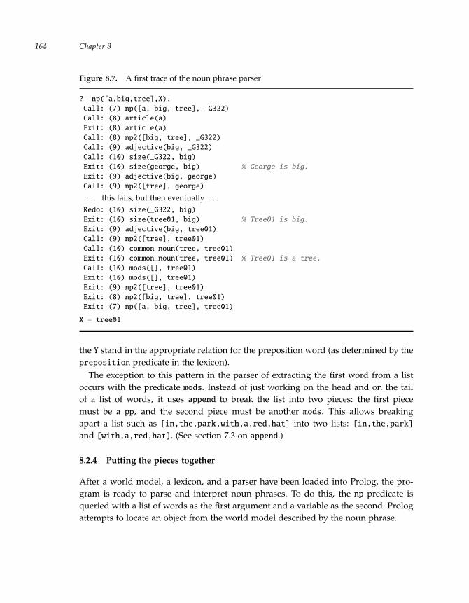
“run” — 2011/9/8 — 18:05 — page 164 — #187�

�

�

�

�

�

�

�

Chapter 8164

Figure 8.7. A first trace of the noun phrase parser

?- np([a,big,tree],X).

Call: (7) np([a, big, tree], _G322)

Call: (8) article(a)

Exit: (8) article(a)

Call: (8) np2([big, tree], _G322)

Call: (9) adjective(big, _G322)

Call: (10) size(_G322, big)

Exit: (10) size(george, big) % George is big.

Exit: (9) adjective(big, george)

Call: (9) np2([tree], george)

. . . this fails, but then eventually . . .Redo: (10) size(_G322, big)

Exit: (10) size(tree01, big) % Tree01 is big.

Exit: (9) adjective(big, tree01)

Call: (9) np2([tree], tree01)

Call: (10) common_noun(tree, tree01)

Exit: (10) common_noun(tree, tree01) % Tree01 is a tree.

Call: (10) mods([], tree01)

Exit: (10) mods([], tree01)

Exit: (9) np2([tree], tree01)

Exit: (8) np2([big, tree], tree01)

Exit: (7) np([a, big, tree], tree01)

X = tree01

the Y stand in the appropriate relation for the preposition word (as determined by thepreposition predicate in the lexicon).

The exception to this pattern in the parser of extracting the first word from a listoccurs with the predicate mods. Instead of just working on the head and on the tailof a list of words, it uses append to break the list into two pieces: the first piecemust be a pp, and the second piece must be another mods. This allows breakingapart a list such as [in,the,park,with,a,red,hat] into two lists: [in,the,park]and [with,a,red,hat]. (See section 7.3 on append.)

8.2.4 Putting the pieces together

After a world model, a lexicon, and a parser have been loaded into Prolog, the pro-gram is ready to parse and interpret noun phrases. To do this, the np predicate isqueried with a list of words as the first argument and a variable as the second. Prologattempts to locate an object from the world model described by the noun phrase.

“run” — 2011/9/8 — 18:05 — page 165 — #188�

�

�

�

�

�

�

�


Figure 8.8. A second trace of the noun phrase parser

?- np2([woman,beside,mary],W).

Call: (9) np2([woman, beside, mary], _G313)

Call: (10) common_noun(woman, _G313)

Exit: (10) common_noun(woman, mary) % The first woman: mary

Call: (10) mods([beside, mary], mary)

. . . this fails and then . . .Redo: (10) common_noun(woman, _G313)

Exit: (10) common_noun(woman, linda) % The second woman: linda

Call: (10) mods([beside, mary], linda) % Break into two pieces:

Call: (11) pp([], linda) % [] and [beside,mary]? No.

Call: (11) pp([beside], linda) % [beside] and [mary]? No.

Call: (11) pp([beside, mary], linda) % [beside,mary] and []?

Call: (12) preposition(beside, linda, _L720)

Exit: (12) preposition(beside, linda, mary)

Call: (12) np([mary], mary) % This succeeds.

Call: (11) mods([], linda), % This succeeds, too.. . . and eventually . . .Exit: (9) np2([woman, beside, mary], linda)

W = linda

A partial trace for the words [a,big,tree] is shown in figure 8.7. Observe that np2must locate something that is big and that is also a tree. In looking for something big(via adjective and then size), it first locates george, but then eventually backtracksand settles on tree01, which passes the remaining test.

A more complex trace for the words [woman,beside,mary] as an np2 appears infigure 8.8. The process is the same, but there are many more steps. In looking for awoman, the parser first comes up with Mary. But Mary is not beside Mary, so therest of the parse fails. It then backtracks and finds Linda. At this point, mods needs touse append to break up the sequence of words [beside,mary] into a pp followed byanother mods, as required by the grammar. Here is what happens:

1. The parser uses append to split the list into [] and [beside,mary], but [] is nota pp, so it backtracks and reconsiders.

2. It tries [beside] and [mary], but [beside] is not a pp either.

3. It gets to [beside,mary] and [], where [beside,mary] is the pp(that correctly describes Linda) and [] is the remaining mods.

This show how append can be used to divide a list of words into syntactic groups.

“run” — 2011/9/8 — 18:05 — page 166 — #189�

�

�

�

�

�

�

�

Chapter 8166

Figure 8.9. Handling ambiguity in noun phrases

Call: (7) np2([man,in,the,park,with,a,tree],_G334)

Call: (8) common_noun(man,_G334)

Exit: (8) common_noun(man,john)

Call: (8) mods([in,the,park,with,a,tree],john)

Call: (9) pp([],john)

Call: (9) pp([in],john)

Call: (9) pp([in,the],john)

Call: (9) pp([in,the,park],john)

Exit: (9) pp([in,the,park],john) % Part 1: yes.

Call: (9) mods([with,a,tree],john)

Fail: (9) mods([with,a,tree],john) % Part 2: no.

Fail: (9) pp([in,the,park],john)

Call: (9) pp([in,the,park,with],john)

Call: (9) pp([in,the,park,with,a],john)

Call: (9) pp([in,the,park,with,a,tree],john) % A better split.

Call: (10) preposition(in,john,_G335)

Exit: (10) preposition(in,john,kew_beach)

Call: (10) np([the,park,with,a,tree],kew_beach)

Exit: (10) np([the,park,with,a,tree],kew_beach)

Exit: (9) pp([in,the,park,with,a,tree],john)

Exit: (8) mods([in,the,park,with,a,tree],john)

Exit: (7) np2([man,in,the,park,with,a,tree],john)

Although this parser deals mainly with syntactic structure, it is also able to dis-ambiguate certain phrases using the world model. Consider the trace in figure 8.9.The English noun phrase in question is the ambiguous a man in the park with a

tree. Once np2 decides that the man is John, it must confirm using mods that[in,the,park,with,a,tree] describes John. The parser needs to break this into somenumber of prepositional phrases (again using append) that each describe John. Hereis what is seen in the trace:

One possibility is that there are two modifying phrases [in,the,park] and[with,a,tree]. However, while the first one can be used to describe John, thesecond one, [with,a,tree] cannot. So this parse is rejected.

The second possibility is that the entire sequence of words is a single modifyingphrase. For this to work, [the,park,with,a,tree] must be a noun phrase thatrefers to kew_beach, since that is where John is located. This works out.

So while the English phrase is ambiguous as to whether with a tree modifies man orpark, the parser uses semantic considerations to reject the first of these interpretations.

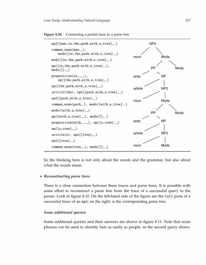
“run” — 2011/9/8 — 18:05 — page 167 — #190�

�

�

�

�

�

�

�


Figure 8.10. Connecting a partial trace to a parse tree

np2([man,in,the,park,with,a,tree],_)

common_noun(man,_),mods([in,the,park,with,a,tree],_)

mods([in,the,park,with,a,tree],_)

pp([in,the,park,with,a,tree],_),mods([],_)

preposition(in,_,_),np([the,park,with,a,tree],_)

np([the,park,with,a,tree],_)

article(the), np2([park,with,a,tree],_)

np2([park,with,a,tree],_)

common_noun(park, ), mods([with,a,tree], )

mods([with,a,tree],_)

pp([with,a,tree],_), mods([],_)

preposition(with,_,_), np([a,tree],_)

np([a,tree],_)

article(a), np2([tree],_)

np2([tree],_)

common_noun(tree,_), mods([],_)

NP2

Mods

ModsPP

NP

NP2

Mods

PP Mods

NP

NP2

Mods

noun

prep

article

noun

prep

article

noun

So the thinking here is not only about the words and the grammar, but also aboutwhat the words mean.

∗ Reconstructing parse trees

There is a close connection between these traces and parse trees. It is possible withsome effort to reconstruct a parse tree from the trace of a successful query to theparser. Look at figure 8.10. On the left-hand side of the figure are the Call parts of asuccessful trace of an np2; on the right, is the corresponding parse tree.

Some additional queries

Some additional queries and their answers are shown in figure 8.11. Note that nounphrases can be used to identify hats as easily as people, as the second query shows.

“run” — 2011/9/8 — 18:05 — page 168 — #191�

�

�

�

�

�

�

�

Chapter 8168

Figure 8.11. More queries over noun phrases

?- np([a,man,with,a,big,hat],X).

X = george ;

No

?- np([the,hat,on,george],X).

X = hat04 ;

No

?- np([a,man,in,a,park,with,a,big,tree],X).

No

?- np([a,woman,in,a,park,with,a,big,tree],X).

X = mary ;

X = linda ;

No

?- np([a,woman,in,a,park,with,a,big,red,hat],X).

X = linda ;

No

?- np([a,woman,beside,a,woman,with,a,blue,hat],X).

X = mary ; % This is not the obvious reading.

X = linda ; % This is the obvious reading.

No

?- np([a,woman,with,a,blue,hat,beside,a,woman],X).

X = mary ;

No

The third and fourth queries reveal that there are no men in a park with a big tree,but there are two women there. The fifth query brings the result that Linda is the onlywoman in a park with a big red hat.

Given this information, observe in the sixth query the handling of the noun phrasea woman beside a woman with a blue hat. This phrase is ambiguous, although themore common interpretation is to attach a blue hat to the second woman mentioned,in which case the entire phrase refers to Linda (who is wearing a red hat). If onewanted to attach both prepositional phrases to the first woman, one would normallyuse a noun phrase like a woman with a blue hat beside a woman (as in the final query),which can only refer to Mary.

Generating noun phrases

Figure 8.12 shows what happens with the np predicate when variables are put intothe noun phrase part of the query:

“run” — 2011/9/8 — 18:05 — page 169 — #192�

�

�

�

�

�

�

�


Figure 8.12. Some other uses of noun phrases

?- np([the,Word,on,john], hat01).

Word = hat ;

No

?- L=[_,_,_,_,_], np(L,linda), \+ member(the,L).

L = [a, small, small, small, woman] ;

L = [a, small, woman, in, queens_park] ;

L = [a, small, woman, beside, mary] ;

L = [a, small, woman, with, hat03] ;

L = [a, small, woman, with, mary] ;

L = [a, woman, in, a, park] ;

L = [a, woman, beside, a, woman] ;

L = [a, woman, with, a, hat] ;

L = [a, woman, with, a, woman] ;

No

?- np(L,linda).

L = [linda] ;

ERROR: Out of local stack % Making ’a small small small ...’

1. The first query looks for a single missing word within a given phrase such thatthe entire phrase would refer to hat01. The word is hat.

2. The second query asks for a noun phrase L with five words that refers to Lindaand does not contain the word the. There are nine such phrases. (Note that asmall small small woman means the same thing here as a small woman.)

3. The third query asks for a noun phrase L that refers to Linda without any furtherrestrictions. It generates the first answer, which is the proper noun linda. Butafter this, it must generate an article followed by an NP2. The first clause of thenp2 predicate is recursive, since an NP2 can be an adjective followed by anotherNP2. Unfortunately, the program gets stuck in a loop here, attempting to generatea sequence of adjectives describing Linda, never making it to the second clauseof the np2 predicate, where a common noun is required.

The third query is an example of trying to go through an infinite set of candidates,which can be problematic (see the discussion of member and append in section 7.3).

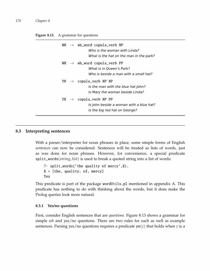
“run” — 2011/9/8 — 18:05 — page 170 — #193�

�

�

�

�

�

�

�

Chapter 8170

Figure 8.13. A grammar for questions

WH → wh_word copula_verb NP

Who is the woman with Linda?

What is the hat on the man in the park?

WH → wh_word copula_verb PP

What is in Queen’s Park?

Who is beside a man with a small hat?

YN → copula_verb NP NP

Is the man with the blue hat John?

Is Mary the woman beside Linda?

YN → copula_verb NP PP

Is John beside a woman with a blue hat?

Is the big red hat on George?

8.3 Interpreting sentences

With a parser/interpreter for noun phrases in place, some simple forms of Englishsentences can now be considered. Sentences will be treated as lists of words, justas was done for noun phrases. However, for convenience, a special predicatesplit_words(string, list) is used to break a quoted string into a list of words:

?- split_words(’the quality of mercy’,X).

X = [the, quality, of, mercy]

Yes

This predicate is part of the package wordUtils.pl mentioned in appendix A. Thispredicate has nothing to do with thinking about the words, but it does make theProlog queries look more natural.

8.3.1 Yes/no questions

First, consider English sentences that are questions. Figure 8.13 shows a grammar forsimple wh and yes/no questions. There are two rules for each as well as examplesentences. Parsing yes/no questions requires a predicate yn(z) that holds when z is a

“run” — 2011/9/8 — 18:05 — page 171 — #194�

�

�

�

�

�

�

�


Figure 8.14. A parser for yes/no questions yesno.pl

yes_no(String) :-

split_words(String,Words), % Get the list of words.

yn(Words). % Use yn on the words.

yn([Verb|Rest]) :-

Verb=is, % The first word must be "is".

append(W1,W2,Rest), % Break the rest into two parts.

np(W1,Ref), % The first part must be an NP.

np_or_pp(W2,Ref). % The second part must be an NP or a PP.

np_or_pp(W,Ref) :- np(W,Ref).

np_or_pp(W,Ref) :- pp(W,Ref).

list of words that forms a yes/no question and whose answer is yes. (A predicate forwh questions is not discussed here.)

A Prolog program for the yn predicate is shown in figure 8.14. It uses append to splitthe list of words after the word is into two groups, where the first must be a nounphrase, and the second is either a noun phrase or a prepositional phrase. It works byfinding a referent for the first group and checking that it can also be a referent for thesecond group. The yes_no predicate is similar, except that it takes a quoted string asits argument. Here are some examples of its use:

?- yes_no(’is mary in a park with linda’).

Yes

?- yes_no(’is the man with the blue hat john’).

No

?- yes_no(’is the big red hat on the woman beside mary’).

Yes

?- yes_no(’is a red with a woman hat’). % Ungrammatical

No

Note that this predicate returns success only if the object described by the first nounphrase is the same as the object described by the second (noun or prepositional)phrase. So with this predicate one cannot distinguish between a failure (a questionthat is ungrammatical or where no referent can be found) and a well-formed questionto which the answer happens to be no.

“run” — 2011/9/8 — 18:05 — page 172 — #195�

�

�

�

�

�

�

�

Chapter 8172

8.3.2 Dynamic predicates in Prolog

Section 8.3.3 deals with declarative sentences. There, instead of being used to query theworld model, a declarative sentence is used to update it. In other words, a declarativesentence is interpreted as providing new information that needs to be incorporated intothe world model.

Prolog allows the clauses associated with some of the predicates to be changedby a program itself. These are called dynamic predicates. For example, suppose apredicate my_pred(x,y,z) takes three arguments. To make that predicate dynamic, aspecial Prolog declaration dynamic is used. The line

:- dynamic my_pred/3.

is included in the program file before my_pred is used. The clauses in the file can thendefine my_pred as usual, but there are also two special Prolog operations, assert andretract, which can be used in queries or in the bodies of clauses:

assert(atom)This query always succeeds; it has the effect of adding the atom as a clause toProlog’s knowledge base.

retract(atom)This query has the effect of removing the first clause in Prolog’s knowledge basethat matches the atom. It fails if there is no match.

So Prolog programs can be written as follows:

get_married(X) :-

retract(single(X)), % X is no longer single.

assert(married(X)). % X is now married.

Predicates like this can be used to keep a model of a changing world up-to-date. Sofor example, if a program with this predicate is loaded together with a world modelthat contains the fact that John is single, the following behavior results:

?- single(john).

Yes

?- get_married(john).

Yes

?- single(john).

No

?- married(john).

Yes

“run” — 2011/9/8 — 18:05 — page 173 — #196�

�

�

�

�

�

�

�


This change to John’s status happens only within the Prolog session. The file with theworld model remains unchanged. This means that if the programmer exits, restartsProlog, and then reloads the file, John’s status will again show as single. To keepJohn’s married status as a permanent part of the world model, the knowledge base ofclauses would have to be saved to a new file, which the program could then run.

8.3.3 Simple declarative sentences

For simplicity, consider declarative sentences described by the following singlegrammar rule:

SD → NP copula_verb preposition NP

This is a special case of the sentences described by the S category of the grammar infigure 8.1. An example sentence of this form is the following:

The man with the red hat is in the park with the big tree.

Parsing sentences like these requires a predicate sd(z) that holds when z is a list ofwords that forms a simple declarative sentence. In addition, the parser should findthe objects corresponding to the two noun phrases, and update the world model. Forthe example sentence shown here, it should assert in(john,queens_park).

To parse and interpret declaratives in this way, prepositions must be used dynam-ically, not just to locate objects in the world model. The simplest way to do this is toextend the lexicon to include a predicate add_for_preposition that states how newinformation for each preposition should be handled:

add_for_preposition(on,X,Y) :- assert(on(X,Y)).

add_for_preposition(in,X,Y) :- assert(in(X,Y)).

add_for_preposition(beside,X,Y) :-

assert(beside(X,Y)), assert(beside(Y,X)).

Note that the assertions for beside give both orders of arguments, since that is theconvention in the world model (for example, for Linda and Mary). Note also thatthere is no clause for the preposition with. This is because of its ambiguity: given thestatement X is with Y, it is not clear what relation should be updated.

With clauses like these in the lexicon, simple declarative sentences can be handledusing the program in figure 8.15. The split_words predicate is used to break a quotedstring into a list of words. The sd predicate takes this list of words and uses appendto break it into a noun phrase, the constant is, a single word Prep (which mustbe a preposition), and a second noun phrase. The predicate np is used to find eachreferent, and the predicate add_for_preposition is used to change the world model.

“run” — 2011/9/8 — 18:05 — page 174 — #197�

�

�

�

�

�

�

�

Chapter 8174

Figure 8.15. A parser for declaratives declarative.pl

simple_declarative(String) :-

split_words(String,Words), % Get words from string.

sd(Words). % Use sd on the words.

sd(Words) :-

append(NP1,[is,Prep|NP2],Words), % Split words.

np(NP1,X), % Find referent for first NP.

np(NP2,Y), % Find referent for second NP.

add_for_preposition(Prep,X,Y). % Add new atom to database.

No attempt is made here to ensure that the new information is reasonable, however.(As it stands, for example, people could end up being located at more than one place.)

8.4 Nonreferential noun phrases

The sort of natural language processing described in this chapter is really just thestart. What makes language so interesting is that it can be used in ways that are muchmore versatile than hinted at here.

For both the interrogative and declarative sentences that have been examined, nounphrases were used to refer to some known individual in the world model. But not allnoun phrases are referential in this sense.

Consider the following: a man without a hat. This is like previous noun phrasesusing the preposition without. However, in this example, the noun phrase a hat is notused referentially; it would be a mistake to look in the world model for the hat thatis being referred to. Indeed, the reference is to a man for whom there is no such hat.(The program clearly needs to be redesigned with respect to prepositional phrasesthat start with the word without.)

Similarly, for the sentence Mary eats an apple every day, one should not look for theobject referred to by the noun phrase an apple. There is no single object that Maryeats over and over; each day it is a different one. The following sentence, on the otherhand, is semantically ambiguous: John wants to marry a rich lawyer. The phrase a rich

lawyer may be referential in designating somebody (say, Susan) whom John wantsto marry and who happens to be a rich lawyer. Or it may be nonreferential in thatthere is no particular individual that John has in mind: whoever it will turn out to be,however, he wants her to be both rich and a lawyer.

“run” — 2011/9/8 — 18:05 — page 175 — #198�

�

�

�

�

�

�

�


Want to read more?

This chapter looked at the thinking behind parsing and interpreting expressions in anatural language.

While there is a long tradition of studying grammar and parsing in classrooms, itis primarily in the work of Noam Chomsky on what is called transformational grammarstarting in the late 1950s that the study of syntax took on a new mathematical preci-sion and generality of description [41]. Chomsky is also well known for having firstproposed a solution to the puzzle of how young children could learn the languageof their parents after being exposed to so few sentences. His proposal is that we areactually born with a universal grammar that allows us to adapt very quickly to theactual grammar of the sentences we first hear.

The approach to semantics in this chapter, which seeks to query or update a sepa-rate knowledge base of facts about the world, owes much to the work of the computerscientist Terry Winograd. His doctoral thesis [43] at MIT in the early 1970s was a muchmore elaborate version of what was considered here, in a world of blocks. To get aglimpse of the major developments in computational linguistics since then, consultthe textbook by Jurafsky and Martin [42].

It needs to be emphasized that the discussion in this chapter only scratches thesurface of how natural language can be used and the kind of thinking that goes onbehind it. The few examples presented here may have given the impression that theprimary purpose of language is to provide information or to request it. In fact, evena casual study of how people actually use language will reveal that this is but a smallpart of the overall picture.

It was the philosopher John Austin in the 1950s who first observed that theimportant thing about language is that people perform language actions (informing,warning, lying, threatening, promising, and so on) to further their goals [40]. Some-times these goals involve information, but often they are quite different. A speakermight be interested, for example, in having a door closed. One way of achieving thatis to get up and close it; another way, in the right circumstances, is to utter somewords like, “Can you close the door?” (clearly not expecting a yes/no answer) oreven “Door, please.” This suggests that the thinking behind language actually hasmuch in common with the thinking about how to achieve goals using actions, whichis the topic of chapter 9.

“run” — 2011/9/8 — 18:05 — page 176 — #199�

�

�

�

�

�

�

�

Chapter 8176

Figure 8.16. A robot arm and some blocks

C

D

EB F

��

G

��

A

��

However, even if language is about using words to achieve goals, it is sometimesfar from clear what those goals are, or how the words contribute to achieving them.Consider a conversation like this:

“Hey! How is it going?”“Not bad. Not bad. How about you?”“Oh, could be worse. I can’t wait for winter to be over.”“You and me both!”

This kind of chit-chat could be ignored if it didn’t make up such a large part oflanguage behavior. What is going on here appears to have little to do with detailsabout the weather (or the sport scores, or the latest celebrity scandal). It’s much morelike a dance where the two parties exchange stylized moves and indicate a willingnessto act together. From an evolutionary point of view, it seems that language behaviorarose out of a strong desire for social interaction of this sort and that all the rest of it(beyond the chit-chat) is more like an interesting offshoot.

Exercises

These exercises put what you have learned about natural language into practice in anew domain. Imagine a robot that is capable of picking up and moving blocks locatedon a table in front of it, as in figure 8.16.

The goal is to tell the robot what to do using ordinary English imperative sen-tences like, “Pick up the pyramid beside the small green cube and put it directly infront of the yellow block.” To interpret English sentences like these, you need to con-struct a world model of facts about this world, a lexicon with all the necessary Englishvocabulary, and a parser/interpreter to process the English expressions.

“run” — 2011/9/8 — 18:05 — page 177 — #200�

�

�

�

�

�

�

�


Before using English words, you will need to build a simple world model of factsabout this blocks world in Prolog. Each block can be assumed to have a color, asize, and a certain shape (a cube, a pyramid, a wedge, . . . ). Also, each block islocated somewhere in the scene. To simplify matters, suppose that the robot livesin a two-dimensional world with these properties:

A block is located either on the table or on another block.

Each block is on at most one other block (which must be a cube) and has at mostone other block directly on it.

The surface of the table is divided into some number (say, 5) of contiguous areas,ordered from left to right.

Each block on the table is located in exactly one of these areas, and each tablearea has at most one block directly on it.

With these assumptions, the locations of blocks can then be represented using a Prologpredicate located_on(block,location), where block is a block and location is either a cubeor one of the table areas. Then a second Prolog predicate area_left_of(area1,area2) isused to state that area1 is the area on the table immediately to the left of area2.

1. Build a world model that expresses basic facts about colors, sizes, shapes,and locations of some blocks in a scene. Include within your documentationa drawing of the blocks-world scene that corresponds to that world model.

2. Write clauses defining the predicates beside(x, y), which holds when block xand y are both on the table in two adjacent areas, and above(x, y), which holdswhen block x is somewhere above block y.

3. Show that your world model works properly by getting Prolog to answer somequeries about it. (These queries should not use English noun phrases.)

Once your world model is working satisfactorily, you are ready to consider Englishnoun phrases and the blocks they refer to in your scene. Here are some examplequeries using English noun phrases:

– np([a,wedge],B).

– np([any,small,green,block],B).

– np([a,pyramid,on,a,big,cube],B).

– np([a,cube,beside,the,orange,wedge],B).

– np([a,cube,below,an,orange,wedge,on,a,red,block],B).(This is ambiguous: is it the cube or the wedge that is on the red block?)

“run” — 2011/9/8 — 18:05 — page 178 — #201�

�

�

�

�

�

�

�

Chapter 8178

– np([a,green,wedge,above,a,block,beside,the,small,red,pyramid],B).

4. Build a Prolog lexicon of articles, adjectives, common nouns, and prepositions,including all the words in the six example noun phrases. The word any shouldbe treated as an article.

5. Copy the Prolog parser/interpreter for noun phrases presented in the chapter(or write your own). Then test the np predicate on a variety of noun phrases toshow that it is capable of identifying the blocks being referred to in your scene.

To model moving a block within your blocks world, suppose there is a predicateput_on(block1, block2) that uses the Prolog assert and retract operations to changethe location of a block. This predicate should fail if the move action would be impos-sible, that is, if there is a block on either block1 or block2, or if block2 is not a cube.Otherwise, put_on should retract the located_on fact involving block1, and assertthat it is now on block2.

6. Write clauses defining the put_on predicate, and test it on a variety of moveoperations. After each operation, include a sketch of what the new scene lookslike, and have your program answer some queries involving that new scene.

7. Extend your parser/interpreter from exercise 5 to handle simple imperative sen-tences of the form “Put NP on NP” where NP is a noun phrase. For example, thefollowing are syntactically well-formed imperative sentences:

Put a green pyramid on the small red cube.Put an orange wedge on the block beside a red cube.Put any small block on a green cube on the big red cube.

The effect of parsing and interpreting sentences such as these should be to updatethe scene using the put_on predicate from exercise 6.

8. Test your parser on a variety of imperative sentences like those in exercise 7,including some that are syntactically well formed but impossible to execute.

9. Show that your grammar for imperative sentences is ambiguous by drawing twoparse trees for the third example sentence in exercise 7. Also show that yourparser can sometimes disambiguate a sentence using facts about the currentscene.

10. Handle the article the properly. The idea here is that a noun phrase like “the redpyramid” should only succeed in naming a block if there is a unique block of theappropriate kind.

“run” — 2011/9/8 — 18:05 — page 179 — #202�

�

�

�

�

�

�

�

9 Case Study: Planning Courses of Action

Intelligent behavior is made intelligent by the application of knowledge. We are ableto act intelligently because we know a lot about the world around us and are ableto bring this knowledge to bear on our decisions about what to do. In particular,we make decisions not just by reacting to what we see, hear, or smell around us butby deliberating about what we want and how to achieve it. For example, instead ofheading toward a file cabinet that contains something we want, we might first thinkabout it and decide to move in a completely opposite direction (if we need to getthe key that will unlock it). As another example, consider the deliberations involvedin a (traditional) wedding: the invitations, the ceremony, the dinner, the reception.Hundreds, even thousands of decisions are pondered well in advance of the weddingday itself. Nobody would call this sort of thinking intellectual, like playing chess ordiscussing Schopenhauer, but it is clearly intelligent behavior of the highest order.

So what is the thinking that underlies these sorts of deliberations? In its simplestform it is planning, contemplating various possible courses of actions, until we findone that we believe will achieve what we want. This is the sort of thinking that isinvestigated in this chapter.

To plan, we need to be able to think about the actions we can take, and imaginewhat the world would be like if we took them. Unlocking a file cabinet will allow adrawer to be opened if the right key is available. Contacting a property manager willallow a wedding planner to discover if a hall can be rented for a reception. Planningis not just thinking about the way the world is but about the way it can be. Thisrequires thinking about the state of the world and how that state is affected by whatwe (and others) do. It is a major intellectual achievement of humans (and no doubtother animals, too) to be able to step back from the world in this manner and imagineit as being quite different from the way it is.

This chapter has four sections. Section 1 discusses two simple but very differentplanning problems and how the planning process is really the same for both of them.Section 2 considers a general planning program in Prolog, and applies it to threeplanning problems. The final two sections consider how planning changes as the

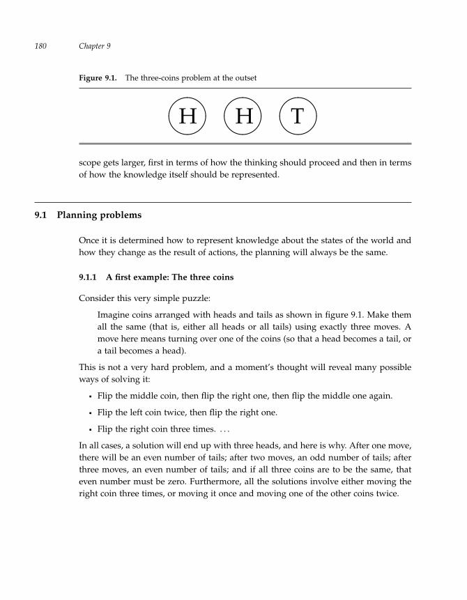
“run” — 2011/9/8 — 18:05 — page 180 — #203�

�

�

�

�

�

�

�

Chapter 9180

Figure 9.1. The three-coins problem at the outset

��H ��

��H ��

��T

scope gets larger, first in terms of how the thinking should proceed and then in termsof how the knowledge itself should be represented.

9.1 Planning problems

Once it is determined how to represent knowledge about the states of the world andhow they change as the result of actions, the planning will always be the same.

9.1.1 A first example: The three coins

Consider this very simple puzzle:

Imagine coins arranged with heads and tails as shown in figure 9.1. Make themall the same (that is, either all heads or all tails) using exactly three moves. Amove here means turning over one of the coins (so that a head becomes a tail, ora tail becomes a head).

This is not a very hard problem, and a moment’s thought will reveal many possibleways of solving it:

Flip the middle coin, then flip the right one, then flip the middle one again.

Flip the left coin twice, then flip the right one.

Flip the right coin three times. . . .

In all cases, a solution will end up with three heads, and here is why. After one move,there will be an even number of tails; after two moves, an odd number of tails; afterthree moves, an even number of tails; and if all three coins are to be the same, thateven number must be zero. Furthermore, all the solutions involve either moving theright coin three times, or moving it once and moving one of the other coins twice.

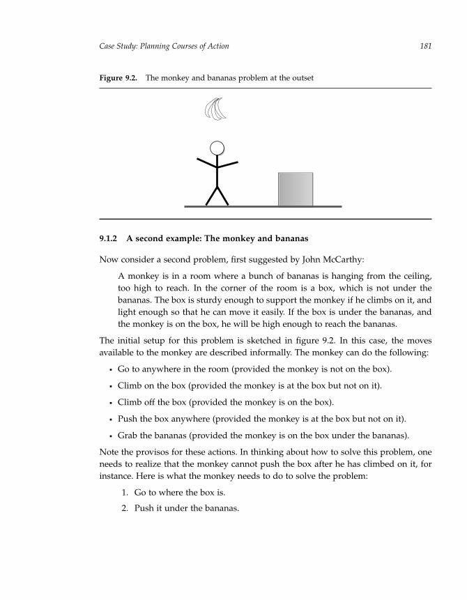
“run” — 2011/9/8 — 18:05 — page 181 — #204�

�

�

�

�

�

�

�

Case Study: Planning Courses of Action 181

Figure 9.2. The monkey and bananas problem at the outset

9.1.2 A second example: The monkey and bananas

Now consider a second problem, first suggested by John McCarthy:

A monkey is in a room where a bunch of bananas is hanging from the ceiling,too high to reach. In the corner of the room is a box, which is not under thebananas. The box is sturdy enough to support the monkey if he climbs on it, andlight enough so that he can move it easily. If the box is under the bananas, andthe monkey is on the box, he will be high enough to reach the bananas.

The initial setup for this problem is sketched in figure 9.2. In this case, the movesavailable to the monkey are described informally. The monkey can do the following:

Go to anywhere in the room (provided the monkey is not on the box).

Climb on the box (provided the monkey is at the box but not on it).

Climb off the box (provided the monkey is on the box).

Push the box anywhere (provided the monkey is at the box but not on it).

Grab the bananas (provided the monkey is on the box under the bananas).

Note the provisos for these actions. In thinking about how to solve this problem, oneneeds to realize that the monkey cannot push the box after he has climbed on it, forinstance. Here is what the monkey needs to do to solve the problem:

1. Go to where the box is.

2. Push it under the bananas.

“run” — 2011/9/8 — 18:05 — page 182 — #205�

�

�

�

�

�

�

�

Chapter 9182

3. Climb on the box.

4. Grab the bananas.

This is not the only way to get the bananas, but it is the most direct.

9.1.3 States and operators

In general, the planning problems in this chapter are characterized by their states andoperators, as follows:

The states of a planning problem are snapshots of the world that are passedthrough while solving the problem. For the two examples, the states are

the sides of the three coins that are showing;

the location of the monkey, the box, and the bananas.

The operators (or moves or actions) of a planning problem are the ways of goingfrom one state to another. For the two examples, the operators are

turning over one of the three coins;

climbing on the box (among others).

The initial state of a planning problem is the state of the problem at the outset.For the two examples, the initial states are

HHT;

as shown in figure 9.2.

The goal state of a planning problem is the desired state (or states) of the problemat the end. For the two examples, the goal states are

HHH or TTT;

any state where the monkey has the bananas.

The planning problems considered in this chapter are always the same: find a wayof going from the initial state of the problem to a goal state by applying a sequenceof operators.

The solution to a planning problem is a plan: a sequence of moves performed inorder, starting from an initial state, and ending at a goal state. In any state along theway it must be possible to apply the current move legally, that is, without violatingany of the given provisos for the move.

“run” — 2011/9/8 — 18:05 — page 183 — #206�

�

�

�

�

�

�

�


9.2 Generating plans

To solve a planning problem using Prolog, the general idea is this:

Represent the initial state, the goal state(s), and the operators of the problem.

The Prolog program will then find a way of getting from the initial state to a goalstate using those operators.

How will it do this? By thinking about the problem, of course! The thoughts will belike this:

If I am in state S and I do move M, that will take me to state S′.From S′ if I now do move M′, that will take me to S′′. . . .

The programmer tells Prolog where to start (that is, the initial state) and where itshould end (the goal state). Along the way, the program will need to keep track of allthe moves it is considering and assemble them into a working plan at the end.

9.2.1 A general planning program

A plan is a sequence of moves from an initial state to a goal state. So the main thing inplanning is knowing how to go from one state S1 to another state S2 using a sequenceof legal moves L. (Bigger planning problems will present much more to think about.)The state S2 is said to be reachable from S1 using L, which is written this way:

S1L−→ S2

There are only two principles to know about this reachability:

S is reachable from S (trivially) using no moves: S〈〉−→ S.

If there is a legal move M0 that goes from state S1 to state S2, and S3 is reachablefrom S2 using moves 〈M1, . . . , Mn〉, then S3 is also reachable from S1 using moves〈M0, M1, . . . , Mn〉. This is represented as follows:

If S1M0−→ S2 and S2

〈M1, ..., Mn〉→ . . . → S3, then S1〈M0, M1, ..., Mn〉→ . . . → S3

A planner can be defined in Prolog by encoding these two reachability principlesdirectly, as shown in figure 9.3. To solve a planning problem, the plan predicate isused to generate a list of moves L such that a goal state G is reachable from the initialstate I using L.

“run” — 2011/9/8 — 18:05 — page 184 — #207�

�

�

�

�

�

�

�

Chapter 9184

Figure 9.3. A general planner in Prolog plan.pl

% This general planner needs the predicates below to be defined:

% - legal_move(BeforeState,Move,AfterState)

% - initial_state(State)

% - goal_state(State)

% plan(L): L is a list of moves from the initial state to a goal state.

plan(L) :- initial_state(I), goal_state(G), reachable(I,L,G).

% reachable(S1,L,S2): S2 is reachable from S1 using moves L.

reachable(S,[],S).

reachable(S1,[M|L],S3) :- legal_move(S1,M,S2), reachable(S2,L,S3).

Figure 9.4. The three-coins problem in Prolog coins.pl

% The three-coins problem formulated for the general planner.

initial_state([h,h,t]).

goal_state([h,h,h]).

goal_state([t,t,t]).

% The three possible moves. Each changes one of the coins.

legal_move([X,Y,Z],flip_left,[X1,Y,Z]) :- opposite(X,X1).

legal_move([X,Y,Z],flip_middle,[X,Y1,Z]) :- opposite(Y,Y1).

legal_move([X,Y,Z],flip_right,[X,Y,Z1]) :- opposite(Z,Z1).

opposite(h,t). % Flipping a head gives a tail.

opposite(t,h). % Flipping a tail gives a head.

This is what is called a general planner. For each specific planning problem to besolved, one must provide clauses that define the initial_state, goal_state, andlegal_move predicates for that problem.

9.2.2 Solving the three-coins problem

To solve a planning problem like the three-coins problem, the first thing to determineis how to represent the states of the problem symbolically. In this case, a state isdetermined by which sides of the coins are showing. So a state of the problem can berepresented using a list with three elements [x,y,z], where the x, y, and z are eitherh (for heads) or t (for tails). (There are eight states in total.)

The full program based on this representation is shown in figure 9.4. Note thesingle initial state and the two possible goal states. The next three clauses definethe legal_move predicate. There are three possible moves: turning over the left, the

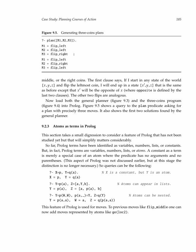
“run” — 2011/9/8 — 18:05 — page 185 — #208�

�

�

�

�

�

�

�


Figure 9.5. Generating three-coins plans

?- plan([M1,M2,M3]).

M1 = flip_left

M2 = flip_left

M3 = flip_right ;

M1 = flip_left

M2 = flip_right

M3 = flip_left

middle, or the right coins. The first clause says, If I start in any state of the world[x,y,z] and flip the leftmost coin, I will end up in a state [x′,y,z] that is the sameas before except that x′ will be the opposite of x (where opposite is defined by thelast two clauses). The other two flips are analogous.

Now load both the general planner (figure 9.3) and the three-coins program(figure 9.4) into Prolog. Figure 9.5 shows a query to the plan predicate asking fora plan with precisely three moves. It also shows the first two solutions found by thegeneral planner.

9.2.3 Atoms as terms in Prolog

This section takes a small digression to consider a feature of Prolog that has not beenstudied yet but that will simplify matters considerably.

So far, Prolog terms have been identified as variables, numbers, lists, or constants.But, in fact, Prolog terms are variables, numbers, lists, or atoms. A constant as a termis merely a special case of an atom where the predicate has no arguments and noparentheses. (This aspect of Prolog was not discussed earlier, but at this stage thedistinction is no longer necessary.) So queries can be the following:

?- X=p, Y=q(a). % X is a constant, but Y is an atom.

X = p, Y = q(a)

?- Y=p(a), Z=[a,Y,b]. % Atoms can appear in lists.

Y = p(a), Z = [a, p(a), b]

?- Y=p(W,W), p(a,_)=Y, Z=q(Y) % Atoms can be nested.

Y = p(a,a), W = a, Z = q(p(a,a))

This feature of Prolog is used for moves. To previous moves like flip_middle one cannow add moves represented by atoms like go(loc2).

“run” — 2011/9/8 — 18:05 — page 186 — #209�

�

�

�

�

�

�

�

Chapter 9186

9.2.4 Solving the monkey and bananas problem

The states in the monkey and bananas problem are more complex than for the three-coins problem. Each state must specify the location of the monkey, bananas and box,and also whether the monkey is on the box, and whether the monkey has the bananas.This suggests using a five-element list [b,m,l,o,h], as follows:

b, m, and l are the locations of the bananas, monkey, and box, respectively.

o is either y or n according to whether the monkey is on the box. (The monkeycan be at the same location as the box but not on it.)

h is either y or n according to whether the monkey has the bananas.

For locations, the easiest thing to do is to name the initial locations of the bananas,monkey, and box as loc1, loc2, and loc3. So, for example, the initial state will be[loc1,loc2,loc3,n,n]. No other location needs to have a name. A goal state will bea five-element list whose last element is y.

The moves available to the monkey are the following:

climb_on (climbing on the box)

climb_off (climbing off the box)

grab (grabbing the bananas)

go(X) (going to location X)

push(X) (pushing the box to location X)

Clauses for legal_move must be written for each of these operators, just as was donefor the operators of the three-coins problem. These clauses should say how a beforestate is transformed to an after state by the operator in question. The clauses shouldfail if the operator in question cannot be used in the before state.

Consider climb_on. It takes a state [b,m,l,o,h] to another state just like it excepto = y. But this move is only legal when the monkey is at the same location as the box(m = l) and when the monkey is not already on the box (o = n):

legal_move([B,M,L,O,H],climb_on,[B1,M1,L1,O1,H1]) :-

M=L, O=n, % Provisos on the old state

B1=B, M1=M, L1=L, O1=y, H1=H. % Values for the new state

This can be written more succinctly as

legal_move([B,M,M,n,H],climb_on,[B,M,M,y,H]).

The climb_off and grab operators will be similar.

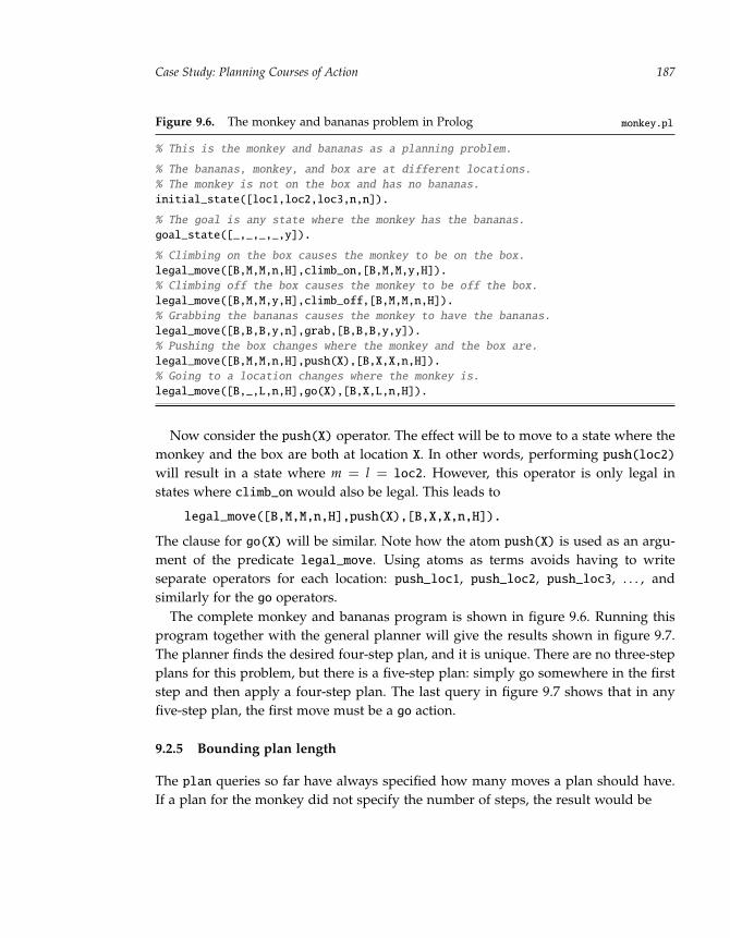
‘‘run’’ --- 2011/9/8 --- 18:05 --- page 187 --- #210�

�

�

�

�

�

�

�


Figure 9.6. The monkey and bananas problem in Prolog monkey.pl

% This is the monkey and bananas as a planning problem.

% The bananas, monkey, and box are at different locations.

% The monkey is not on the box and has no bananas.

initial_state([loc1,loc2,loc3,n,n]).

% The goal is any state where the monkey has the bananas.

goal_state([_,_,_,_,y]).

% Climbing on the box causes the monkey to be on the box.

legal_move([B,M,M,n,H],climb_on,[B,M,M,y,H]).

% Climbing off the box causes the monkey to be off the box.

legal_move([B,M,M,y,H],climb_off,[B,M,M,n,H]).

% Grabbing the bananas causes the monkey to have the bananas.

legal_move([B,B,B,y,n],grab,[B,B,B,y,y]).

% Pushing the box changes where the monkey and the box are.

legal_move([B,M,M,n,H],push(X),[B,X,X,n,H]).

% Going to a location changes where the monkey is.

legal_move([B,_,L,n,H],go(X),[B,X,L,n,H]).

Now consider the push(X) operator. The effect will be to move to a state where themonkey and the box are both at location X. In other words, performing push(loc2)will result in a state where m = l = loc2. However, this operator is only legal instates where climb_on would also be legal. This leads to

legal_move([B,M,M,n,H],push(X),[B,X,X,n,H]).

The clause for go(X) will be similar. Note how the atom push(X) is used as an argu-ment of the predicate legal_move. Using atoms as terms avoids having to writeseparate operators for each location: push_loc1, push_loc2, push_loc3, . . . , andsimilarly for the go operators.

The complete monkey and bananas program is shown in figure 9.6. Running thisprogram together with the general planner will give the results shown in figure 9.7.The planner finds the desired four-step plan, and it is unique. There are no three-stepplans for this problem, but there is a five-step plan: simply go somewhere in the firststep and then apply a four-step plan. The last query in figure 9.7 shows that in anyfive-step plan, the first move must be a go action.

9.2.5 Bounding plan length

The plan queries so far have always specified how many moves a plan should have.If a plan for the monkey did not specify the number of steps, the result would be

“run” — 2011/9/8 — 18:05 — page 188 — #211�

�

�

�

�

�

�

�

Chapter 9188

Figure 9.7. Generating plans for the monkey

?- plan([M1,M2,M3,M4]). % Is there a four-step plan?

M1 = go(loc3)

M2 = push(loc1)

M3 = climb_on

M4 = grab ; % Are there any others?

No

?- plan([M1,M2,M3]). % Is there a three-step plan?

No

?- plan([M1,M2,M3,M4,M5]). % Is there a five-step plan?

M1 = go(_G325) % First go to any location.

M2 = go(loc3) % Then proceed as above.

M3 = push(loc1)

M4 = climb_on

M5 = grab

?- plan([M1,M2,M3,M4,M5]), \+ M1 = go(_).

No

?- plan(L).


The reason for this is that reachable looks for a path from an initial state S0 to a goalstate G. A trace of the query would show the following:

1. The first action is a go action from state S0 to a state S1, so the planner needs tofind a path from S1 to G.

2. The next action is a go action from state S1 to a state S2, so the planner needs tofind a path from S2 to G. . . .

In the end, the planner would look for ever longer sequences of go actions and neverget to the other moves. On the other hand, if the sequence were bounded in advance,for instance, if the planner looked only for plans with four steps, then after fourgo actions, the reachable predicate would fail, and the planner would be forced tobacktrack and consider other actions.

This suggests that it is useful to have a version of the general planner that first tries[], then [_], then [_,_], then [_,_,_], and so on, until it finds a plan. There are afew ways to do this, but perhaps the simplest is shown in figure 9.8. The new generalplanner is called bplan. Its predicate tryplan(x, y) holds if y is a successful plan andis like x but possibly with some additional elements at the front. This predicate works

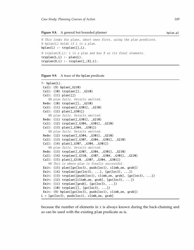
“run” — 2011/9/8 — 18:05 — page 189 — #212�

�

�

�

�

�

�

�


Figure 9.8. A general but bounded planner bplan.pl

% This looks for plans, short ones first, using the plan predicate.

% bplan(L) holds if L is a plan.

bplan(L) :- tryplan([],L).

% tryplan(X,L): L is a plan and has X as its final elements.

tryplan(L,L) :- plan(L).

tryplan(X,L) :- tryplan([_|X],L).

Figure 9.9. A trace of the bplan predicate

?- bplan(L).

Call: (9) bplan(_G210)

Call: (10) tryplan([], _G210)

Call: (11) plan([])

%% plan fails. Details omitted.

Redo: (10) tryplan([], _G210)

Call: (11) tryplan([_G301], _G210)

Call: (12) plan([_G301])


Redo: (11) tryplan([_G301], _G210)

Call: (12) tryplan([_G304, _G301], _G210)

Call: (13) plan([_G304, _G301])


Redo: (12) tryplan([_G304, _G301], _G210)

Call: (13) tryplan([_G307, _G304, _G301], _G210)

Call: (14) plan([_G307, _G304, _G301])


Redo: (13) tryplan([_G307, _G304, _G301], _G210)

Call: (14) tryplan([_G310, _G307, _G304, _G301], _G210)

Call: (15) plan([_G310, _G307, _G304, _G301])

%% This is where plan is finally successful.

Exit: (15) plan([go(loc3), push(loc1), climb_on, grab])

Exit: (14) tryplan([go(loc3), ...], [go(loc3), ...])

Exit: (13) tryplan([push(loc1), climb_on, grab], [go(loc3), ...])

Exit: (12) tryplan([climb_on, grab], [go(loc3), ...])

Exit: (11) tryplan([grab], [go(loc3), ...])

Exit: (10) tryplan([], [go(loc3), ...])

Exit: (9) bplan([go(loc3), push(loc1), climb_on, grab])

L = [go(loc3), push(loc1), climb_on, grab]

because the number of elements in x is always known during the back-chaining andso can be used with the existing plan predicate as is.

‘‘run’’ --- 2011/9/8 --- 18:05 --- page 190 --- #213�

�

�

�

�

�

�

�

Chapter 9190

Figure 9.10. The 15-puzzle

goal stateinitial state

=⇒4321

8765

1211109

1514139 14 11 12

13 5 4

10 2 7 15

1 6 3 8

A partial trace of the bplan predicate in action on the monkey and bananas problemis shown in figure 9.9. Note that if a planning problem cannot be solved, that is, ifthere is no sequence of moves that go from the initial state to a goal state, the bplanpredicate (like the plan predicate) will continue searching indefinitely for ever longersequences of moves.

9.2.6 A third example: The 15-puzzle

This section considers a more substantial planning problem, the 15-puzzle, attributedto Noyes Chapman (and sometimes to Sam Loyd). It is a puzzle that consists of a4× 4 frame containing tiles numbered 1 to 15 placed in random order (with one spaceempty). The object of the puzzle is to place the tiles in numerical order by makingsliding moves that use the empty space. Figure 9.10 shows one possible initial stateand the desired final state.

A state of the puzzle can be represented with a sixteen-element list [p1, p2, . . . , p16],where each pi is a number from 0 to 15 indicating which tile is in position i (and where0 means that position i is empty). For the puzzle in figure 9.10,

the initial state is [1,6,3,8,10,2,7,15,13,5,4,0,9,14,11,12];

the goal state is [1,2,3,4,5,6,7,8,9,10,11,12,13,14,15,0].

The available moves involve sliding a tile up, down, left, or right, according tothe position of the empty space. The corresponding operators are up(X), down(X),left(X), and right(X), where X is a tile.

The easiest way to write legal_move for the up operator is to write a clause for eachof the twelve locations of the empty square where a tile can go up. For example, tohandle a tile X moving up when the empty space is in position 3, one would write thefollowing:

“run” — 2011/9/8 — 18:05 — page 191 — #214�

�

�

�

�

�

�

�


Figure 9.11. A 2 x 3 version of the 15-puzzle puzzle2x3.pl

% This is a 2x3 version of the 15 puzzle. %%%%%%%%%

initial_state([0,1,5,4,3,2]). %----------------------> % 1 5 %

goal_state([1,2,3,4,5,0]). % 4 3 2 %

legal_move([0,B,C, X,E,F],up(X),[X,B,C, 0,E,F]). %%%%%%%%%

legal_move([A,0,C, D,X,F],up(X),[A,X,C, D,0,F]).

legal_move([A,B,0, D,E,X],up(X),[A,B,X, D,E,0]).

legal_move(S1,down(X),S2) :- legal_move(S2,up(X),S1).

legal_move([0,X,C, D,E,F],left(X),[X,0,C, D,E,F]).

legal_move([A,0,X, D,E,F],left(X),[A,X,0, D,E,F]).

legal_move([A,B,C, 0,X,F],left(X),[A,B,C, X,0,F]).

legal_move([A,B,C, D,0,X],left(X),[A,B,C, D,X,0]).

legal_move(S1,right(X),S2) :- legal_move(S2,left(X),S1).

legal_move(S1,up(X),S2) :-

S1=[A,B,0,D, E,F,X,H, I,J,K,L, M,N,O,P],

S2=[A,B,X,D, E,F,0,H, I,J,K,L, M,N,O,P].

Note that nothing changes between the two states except at positions 3 and 7, wherethe empty space and tile X are interchanged. There will be twelve such clauses foreach of the four operators. Writing these is both tedious and error-prone. (This issueis discussed in section 9.4.) However, there is a shortcut because up and down areinverses (as are the left and right operators). Once the necessary clauses for up havebeen written, a single clause for down will suffice:

legal_move(S1,down(X),S2) :- legal_move(S2,up(X),S1).

A complete program for the 2 × 3 version of the puzzle is shown in figure 9.11.Running it gives the following result:

?- bplan(L).

L = [left(1), up(3), left(2), down(5), right(3), up(2), left(5)]

9.3 Scaling up: The search problem

For small planning problems like the three puzzles just considered, the thinkingworks fine. But for more realistic domains, the planning will have to be done in adifferent way. This section reconsiders the thinking process itself; the next section,reconsiders how to better represent the states of a changing world.

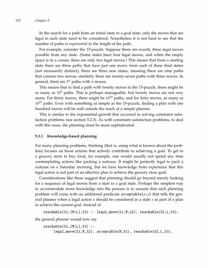
“run” — 2011/9/8 — 18:05 — page 192 — #215�

�

�

�

�

�

�

�

Chapter 9192

In the search for a path from an initial state to a goal state, only the moves that arelegal in each state need to be considered. Nonetheless it is not hard to see that thenumber of paths is exponential in the length of the path.

For example, consider the 15-puzzle. Suppose there are exactly three legal movespossible from any state. (Some states have four legal moves, and when the emptyspace is in a corner, there are only two legal moves.) This means that from a startingstate there are three paths that have just one move; from each of these final states(not necessarily distinct), there are three new states, meaning there are nine pathsthat contain two moves; similarly, there are twenty-seven paths with three moves. Ingeneral, there are 3n paths with n moves.

This means that to find a path with twenty moves in the 15-puzzle, there might beas many as 109 paths. This is perhaps manageable, but twenty moves are not verymany. For thirty moves, there might be 1014 paths, and for forty moves, as many as1019 paths. Even with something as simple as the 15-puzzle, finding a plan with onehundred moves will be well outside the reach of a simple planner.

This is similar to the exponential growth that occurred in solving constraint satis-faction problems (see section 5.2.3). As with constraint satisfaction problems, to dealwith this issue, the planning must be more sophisticated.

9.3.1 Knowledge-based planning

For many planning problems, thinking (that is, using what is known about the prob-lem) focuses on those actions that actively contribute to achieving a goal. To get toa grocery store to buy food, for example, one would usually not spend any timecontemplating actions like packing a suitcase. It might be perfectly legal to pack asuitcase on a Saturday morning, but we have knowledge from experience that thislegal action is not part of an effective plan to achieve the grocery store goal.

Considerations like these suggest that planning should go beyond merely lookingfor a sequence of legal moves from a start to a goal state. Perhaps the simplest wayto accommodate more knowledge into the process is to assume that each planningproblem will come with an additional predicate acceptable(a,s) that tells the gen-eral planner when a legal action a should be considered in a state s as part of a planto achieve the current goal. Instead of

reachable(S1,[M|L],S3) :- legal_move(S1,M,S2), reachable(S2,L,S3).

the general planner would now say

reachable(S1,[M|L],S3) :-

legal_move(S1,M,S2), acceptable(M,S1), reachable(S2,L,S3).

“run” — 2011/9/8 — 18:05 — page 193 — #216�

�

�

�

�

�

�

�


It would then be up to the programmer of each individual planning problem to spec-ify which actions are acceptable for the goal in question and which should be filtered.If it so happens that absolutely nothing is known about how to plan for the goal, theclause

acceptable(_,_). % No filter, so anything goes.

can be included in the problem specification, and the resulting planning behavior isthe same as before.

For the 15-puzzle, imagine that in a current state tiles 1, 2, 3, and 4 are in theircorrect positions in the first row, and that the empty space is below tile 2 (in position6). While it is perfectly legal to move tile 2 down next, experience says that this isnot a good idea: once the first row is in place, it should not be disturbed. A simplefirst step toward using this knowledge in planning would be to filter that action in aprogram for the 15-puzzle, as follows:

acceptable(down(X),S) :- \+ row1_done(X,S).

row1_done(X,S) :- member(X,[1,2,3,4]), S=[1,2,3,4|_].

This would prevent the program from wasting its time considering plans that disturbthe first row once it is in place.

Decomposing a problem

This idea of not disturbing some parts of a goal that have been solved is a general one.Many planning problems have the following property: they are made of subproblemsthat can be solved independently and then combined.

How does this help? Imagine there is a problem that can be solved using twenty-five moves. Assume there are three legal moves at each state; this means that theremight be 325, or about 1012, paths to a goal state.

But suppose that this problem can be broken down into two independent pieces,A and B, where the A part can be solved in ten steps, and the B part can be solvedin the remaining fifteen steps. To solve A, there might be as many as 310 paths, andto solve B, 315 paths, so that in total, there might be (310 + 315), or about 107, pathsto a goal state. But this is much less than 1012 paths. Similarly, if the problem canbe broken down into five independent pieces, each requiring five steps (for a totalof twenty-five), there might be only 5 · 35, or about 103, paths. In general, solvinga problem that can be broken down into independent subproblems requires dealingwith the sum of their search spaces, not the product, an enormous difference.

Many natural problems have this decomposition structure allowing them to behandled effectively. Consider the 15-puzzle again. The goal of getting all the tiles in

“run” — 2011/9/8 — 18:05 — page 194 — #217�

�

�

�

�

�

�

�

Chapter 9194

Figure 9.12. Decomposing the 15-puzzle

first goal second goal third goal

1211

15

876

--10

--14

4321

---5

---9

---13

place breaks down into independent subgoals, as shown in figure 9.12. The first goalis to get the top row and left column of tiles in place without regard for the placementof any of the others. Once this first goal is achieved, the tiles in the top row and leftcolumn are not disturbed, and the second goal can be considered as a 3 × 3 puzzle.The second goal involves getting what is left of the second row and second column inplace, again without regard for the other three tiles. Once this second goal is achieved,the third goal, with the remaining three tiles, is handled as a 2 × 2 puzzle. Note thateach of the goals can be solved independently, as required. Moreover, the first goalitself can be broken down into two independent goals: getting the first row into placeand then getting the remaining three tiles of the first column into place.

∗ Problem decomposition in Prolog

One way to encode this type of problem decomposition in Prolog is to assume that thegeneral planner is given a set of stages that it must pass through to solve a problem.If there is no knowledge at all about how to decompose the problem, there wouldbe exactly two stages: an initial one (applying to every state of the problem) and afinal one (applying to just the goal states). Other problems would have additionalintermediate stages. For example, for the 15-puzzle, the intermediate stages might beone that applies to every state where the first row is in place, another where both thefirst row and first column are in place, and a third where the first two rows and twocolumns are in place. Note that these stages are ordered and that each stage applies toall states of the subsequent stages. This guarantees that as the planner passes througheach stage, it moves ever closer to the final goal.

A Prolog program that plans in stages is shown in figure 9.13. It uses the predicatelegal_move and initial_state as before. But instead of a predicate for goal_state,it expects to see two predicates: stages, which provides a list of the names of the

“run” — 2011/9/8 — 18:05 — page 195 — #218�

�

�

�

�

�

�

�


Figure 9.13. A staged planner in Prolog splan.pl

% This staged planner needs the predicates below to be defined:

% - legal_move(BeforeState,Move,AfterState)

% - initial_state(State)

% - stages(ListofStages)

% - goal_stage(Stage,State)

% plan(L): L is a list of moves through a list of goal stages.

plan(L) :- initial_state(I), stages([G|GL]), plan_all(G,I,L,GL).

% plan_all(G,S,L,GL): L passes from G through each stage in GL.

plan_all(_,_,[],[]).

plan_all(G1,S1,L,[G2|GL]) :-

append(L1,L2,L), reach(G1,S1,L1,G2,S2), plan_all(G2,S2,L2,GL).

% reach(G1,S1,L,G2,S2): L moves from S1 in stage G1 to S2 in G2.

reach(_,S,[],G2,S) :- goal_stage(G2,S). % S attains stage G2.

reach(G1,S1,[M|L],G2,S3) :- % Move from S1 to S2.

legal_move(S1,M,S2), goal_stage(G1,S2), reach(G1,S2,L,G2,S3).

stages that the planner must pass through, and goal_stage(g, s), which holds whenthe stage named g applies to state s. The 15-puzzle might include these clauses:

stages([init,r1,r1c1,r12c12,goal]).

goal_stage(init,_).

goal_stage(r1,[1,2,3,4|_]).

goal_stage(r1c1,[1,2,3,4,5,_,_,_,9,_,_,_,13,_,_,_]).

goal_stage(r12c12,[1,2,3,4,5,6,7,8,9,10,_,_,13,14,_,_]).

goal_stage(goal,[1,2,3,4,5,6,7,8,9,10,11,12,13,14,15,0]).

The way the planner works is to (use append to) break the sequence of moves intoparts that will proceed from stage to stage until all the stages have been attained andthe problem is solved. Whenever it considers a legal move (within the reach predi-cate), it checks that the current stage applies to the state that results from doing themove. This automatically guarantees that the moves within a stage will not compro-mise a subgoal that was previously achieved. (This was handled manually using theacceptable predicate.)

∗ 9.3.2 Best-first search

Once it has been determined that the best one can do is to search for a path fromsome start state to an end state, there are other ways of searching that can be muchmore effective than those used so far. One obvious thing to do is to avoid loops that

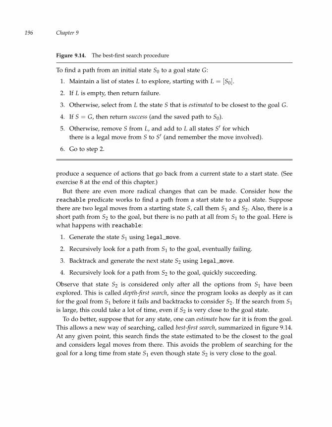
“run” — 2011/9/8 — 18:05 — page 196 — #219�

�

�

�

�

�

�

�

Chapter 9196

Figure 9.14. The best-first search procedure

To find a path from an initial state S0 to a goal state G:

1. Maintain a list of states L to explore, starting with L = [S0].

2. If L is empty, then return failure.

3. Otherwise, select from L the state S that is estimated to be closest to the goal G.

4. If S = G, then return success (and the saved path to S0).

5. Otherwise, remove S from L, and add to L all states S′ for whichthere is a legal move from S to S′ (and remember the move involved).

6. Go to step 2.

produce a sequence of actions that go back from a current state to a start state. (Seeexercise 8 at the end of this chapter.)

But there are even more radical changes that can be made. Consider how thereachable predicate works to find a path from a start state to a goal state. Supposethere are two legal moves from a starting state S, call them S1 and S2. Also, there is ashort path from S2 to the goal, but there is no path at all from S1 to the goal. Here iswhat happens with reachable:

1. Generate the state S1 using legal_move.

2. Recursively look for a path from S1 to the goal, eventually failing.

3. Backtrack and generate the next state S2 using legal_move.

4. Recursively look for a path from S2 to the goal, quickly succeeding.

Observe that state S2 is considered only after all the options from S1 have beenexplored. This is called depth-first search, since the program looks as deeply as it canfor the goal from S1 before it fails and backtracks to consider S2. If the search from S1

is large, this could take a lot of time, even if S2 is very close to the goal state.To do better, suppose that for any state, one can estimate how far it is from the goal.

This allows a new way of searching, called best-first search, summarized in figure 9.14.At any given point, this search finds the state estimated to be the closest to the goaland considers legal moves from there. This avoids the problem of searching for thegoal for a long time from state S1 even though state S2 is very close to the goal.

“run” — 2011/9/8 — 18:05 — page 197 — #220�

�

�

�

�

�

�

�


Of course, for this to work, the programmer must be able to estimate how far astate is from a goal. The estimate does not have to be exact, since it is just a guide towhat state should be explored next.

In the case of the 15-puzzle, there is a natural estimate of how far a state is fromthe goal. In the initial state in figure 9.10, tiles 1 and 3 are in their correct position,but tile 6 has to be moved down one position. Tile 4 has to go up two and right one.The horizontal or vertical distance is known as a Manhattan distance (by analogy withthe grid of streets in Manhattan). So tile 1 has a Manhattan distance of 0 from itshome, tile 6 has a Manhattan distance of 1 from its home, and tile 4 has a Manhattandistance of 2 + 1 = 3 from its home. In general, one can estimate how far a state isfrom the goal by summing the Manhattan distances of every tile from its home. Sothe goal state in figure 9.10 has a distance of 0 from the goal (since every tile is at itshome), and the initial state in figure 9.10 has a distance of

0 + 1 + 0 + 1 + 2 + 1 + 0 + 3 + 1 + 2 + 3 + 1 + 0 + 1 + 1 = 17

from the goal. Note that this estimate has the nice property that it is a lower bound onthe number of moves required to get to a goal state: at the very least, each tile hasto do that number of horizontal or vertical moves to get it to its home. The actualnumber of moves to get to a goal state will typically be much larger, since the tiles getin each other’s way.

9.4 Scaling up: The representation problem

For planning problems like the three small puzzles considered up to now, the methodof representing a state worked just fine. A state was represented as a list whoseelements were the various aspects of the problem, such as the visible side of a coin,the location of the monkey, or the position of a tile in a rectangular frame. But formore realistic domains, it becomes very awkward to deal with lists that include allthe relevant aspects of that domain.

For example, imagine a world with 1,000 boxes that can be moved independently.Representing this state requires a list like [loc1, loc2, loc3, . . . , loc1000]. Then 1,000clauses would be needed to describe the legal_move predicate, one for each boxin the list. The clause would change the location of that box and leave the values ofall the others unchanged, using 999 Prolog variables.

This is not just a problem with locations. In general, even in domains with manyaspects, each action will change only a few of them. Pushing a box under the bananaswill change the location of the monkey and the box, but it will not affect the location

“run” — 2011/9/8 — 18:05 — page 198 — #221�

�

�

�

�

�

�

�

Chapter 9198

of the bananas, the color of the bananas, any other objects in the room, whether ornot doors are open, the temperature in the room, the weather outside, the studentsenrolled at a nearby university, the price of tea in China, and so on.

What is needed is a representation of the state of the world that is more explicitabout what aspects of the world are affected by what actions. The dynamic pred-icates considered in section 8.3.2 had this desirable property. One could startwith single(john) in the knowledge base, for example, then use the predicateget_married(john) in a query, and end up with married(john), quite independentlyof any other predicates. Unfortunately, dynamic predicates cannot be used as is forplanning. They allow changing the state by changing the knowledge base, but theydo not yield sentences that talk about the before and after states simultaneously, whichis what is needed for legal_move.

This section considers a new way to represent the state of the world that is suitablefor planning but makes it possible to talk explicitly about changing aspects of theworld, like the marital status of John or the location of the box.

9.4.1 Situations and fluents

The purpose of a state in planning is to keep track of the relevant aspects of the worldand how these are affected by actions. Instead of representing these aspects in a biglist, another approach is to make a list of all the actions that have been performed, andthen to calculate from this list any relevant aspect.

For example, suppose there is a list of all the actions performed in the monkey andbananas world, and one wants to calculate the location of the box from this list. Thethinking can go as follows:

If there is no push action in the list, then the box will be located wherever it wasin the initial state.

If there are push actions in the list, and the most recent one performed ispush(loc6), then the box will be located at loc6.

So the location of the box is fully determined by a history of all the actions performed,which is called a situation.

A situation is an ordered list of actions used to represent a state of the world. Theactions will appear in this list most recent ones first. For example,

[] is the initial situation, before any action has been performed;

[a] is the situation after the single action a has been performed;

“run” — 2011/9/8 — 18:05 — page 199 — #222�

�

�

�

�

�

�

�


[b,a,a] is the situation where action a was performed twice and then action bwas performed, b being the most recent action.

Note that the situation [a,b] is not the same situation as [b,a]; it might make adifference which action is done first. For example, it is quite different to climb on thebox before grabbing the bananas than to grab for the bananas before climbing on thebox.

Using Prolog notation, performing action A in situation S (which must be a list ofactions) always results in the situation [A|S], since the most recent action is listed atthe head of the list.

With this representation of a state, the various relevant aspects in our world arerepresented as predicates that take a situation as an argument. Such predicates arecalled fluents. (By convention, the situation is the final argument of the fluent.) Soinstead of using a predicate like location(x,l), a final argument is added to make itlocation(x,l,s), which is read as “item x is at location l in situation s.” Informally,all the following sentences involving this fluent should work out to be true:

location(box,loc3,[]) (the initial location of the box)

location(box,loc3,[go(loc3)])

location(box,loc5,[push(loc5),go(loc3)])

location(box,loc5,[go(loc1),push(loc5),go(loc3)])

location(box,loc5,[go(loc7),

go(loc1),push(loc5),go(loc3)])

location(box,loc5,[go(loc5),go(loc7)


location(box,loc4,[push(loc4),go(loc5),go(loc7)


location(box,loc4,[go(loc2),push(loc4),go(loc5),go(loc7)


Note how the most recent push action in the situation determines where the box islocated (from loc3 to loc5 to loc4). After a push, the location of the box stays whereit is as other actions are performed (here, they are all go actions, but they could beanything), until another push changes it again. The job is to write clauses for thelocation fluent so that all these queries succeed.

“run” — 2011/9/8 — 18:05 — page 200 — #223�

�

�

�

�

�

�

�

Chapter 9200

Initial and successor state clauses

The easiest way to characterize a fluent in a program is to do it in two steps:

1. State what holds in the initial situation, []. This is writing what are called theinitial state clauses for the fluent.

2. State what holds in a noninitial situation, [A|S]. This is writing what arecalled the successor state clauses for the fluent. Typically, there are cases involveddepending on the action A and according to whether

a. A makes the fluent true;

b. A makes the fluent false;

c. A leaves the fluent unchanged, as it was in situation S.

Here are the three clauses that characterize the location of the box in any situation:

location(box,loc3,[]).

location(box,L,[push(L)|_]).

location(box,L,[A|S]) :- \+ A=push(_), location(box,L,S).

The first clause is the initial state clause stating that the box is initially located atloc3. (The remaining clauses are the successor state clauses.)

The second clause states that if the most recent action in a situation is pushing thebox to L, then the location of the box is L, no matter what the previous actions inthe situation are. Note that it is not the job of the successor state axiom to ensurethat the push is legal.

The third clause states that if the location of the box in a situation S is L, then thelocation of the box in situation [A|S] (in other words, after doing action A) is alsoL, provided A is not a push action. Note that this provides a recursive definitionof location: to calculate the location of the box in situation [A|S], one may needto calculate the location of the box in situation S.

It is not hard to see that these three clauses will allow all the previous locationsentences to succeed as queries.

This pattern can be applied to other fluents in the monkey and bananas world. Forexample, one would want a fluent on_box to indicate whether or not the monkey ison the box. Climbing on the box makes it true; climbing off the box makes it false; allthe other actions leave this fluent unchanged. In other words,

on_box([climb_on|_]).

on_box([A|S]) :- \+ A=climb_off, on_box(S).

“run” — 2011/9/8 — 18:05 — page 201 — #224�

�

�

�

�

�

�

�


The monkey is on the box if it has just climbed on the box or if it was already on it anddid not just climb off. To characterize a person as being married or single, the patternwill be exactly the same except that getting married makes being married true, andgetting divorced makes it false:

married(X,[get_married(X)|_]).

married(X,[A|S]) :- \+ A=get_divorced(X), married(X,S).

There might be a fluent that can be made true and then stays true thereafter. Forexample, there was no action in this world for the monkey to dispose of the bananasafter grabbing them. So the following successor state clauses apply:

has_bananas([grab|_]).

has_bananas([_|S]) :- has_bananas(S).

Once the monkey has performed a grab action, it has the bananas and will continueto have them no matter what action is performed next. Similarly, in this world, thelocation of the bananas is unaffected by any action:

location(bananas,loc1,[]). % The initial location

location(bananas,L,[_|S]) :- location(bananas,L,S).

More concisely, the location of the bananas can be characterized as being the same asthe initial location in all situations:

location(bananas,loc1,_).

The final fluent needed is the location of the monkey. This is just like the location ofthe box, except that it is affected by both push and go actions:

location(monkey,loc2,[]).

location(monkey,L,[push(L)|_]).

location(monkey,L,[go(L)|_]).

location(monkey,L,[A|S]) :-

\+ A=push(_), \+ A=go(_), location(monkey,L,S).

In other words, the monkey is at a location if it just went or pushed the box there, orif it was already there and did not just go or push the box to somewhere else.

Action precondition clauses

The only thing left to do to fully characterize a world in terms of situations andfluents is to state the conditions under which it is possible to perform an action. Thiswas done implicitly in the legal_move predicate, but here it is useful to state these

“run” — 2011/9/8 — 18:05 — page 202 — #225�

�

�

�

�

�

�

�

Chapter 9202

properties separately using a special predicate poss(a,s), which is interpreted assaying that a is a possible action to perform in situation s.

Here are the clauses for poss in the monkey and bananas world:

poss(climb_off,S) :- on_box(S).

poss(go(_),S) :- \+ on_box(S).

poss(grab,S) :-

on_box(S), location(box,L,S), location(bananas,L,S).

poss(push(_),S) :- poss(climb_on,S).

poss(climb_on,S) :-

\+ on_box(S), location(box,L,S), location(monkey,L,S).

Clauses like these are called action precondition clauses. Note how they use the fluentsto state when it is possible to perform an action. For example, the monkey can climbon the box only when it is located at the same place as the box and is not already onit. A push action is only possible under the same conditions.

This completes the representation of the monkeys and bananas world usingsituations and fluents.

9.4.2 Planning with situations and fluents

After all the initial state, successor state, and action precondition clauses for someworld have been written, the planning can begin. Recall that for the plan (or bplan)predicate, one must provide three problem-specific predicates: initial_state,goal_state, and legal_move. With situations and fluents, this is very easy:

initial_state([]).

legal_move(S,A,[A|S]) :- poss(A,S).

goal_state(S) :- has_bananas(S).

The initial state is always the same for any problem: it is the initial situation, theempty list. Similarly, the legal_move clause is always the same: one can move fromsituation S to situation [A|S] for any action A for which poss holds. Only the goalstate varies from problem to problem; for the monkey and bananas, it is any situationwhere the monkey has the bananas.

So if these three clauses are added to the characterization of the monkey andbananas world in terms of situations and fluents, the plan predicate can be usedto find the four-step plan as before.

“run” — 2011/9/8 — 18:05 — page 203 — #226�

�

�

�

�

�

�

�


9.4.3 Why is this representation useful?

Representing the monkeys and bananas world using situations and fluents mightseem like a lot of effort for very little benefit. There was already a less verbose andquite workable characterization of this world for planning (figure 9.6). So why bother?The answer is that, in general, a representation in terms of situations and fluents hasone significant advantage:

A representation in terms of situations and fluents allows characterizing part of aworld without having to know in advance all the other actions and fluents.

Consider again the fluent on_box, for example. Once the actions affecting this fluentare identified, one can write the successor state clauses:

on_box([climb_on|_]).

on_box([A|S]) :- \+ A=climb_off, on_box(S).

Even if it later becomes important to keep track of a new aspect, say, the color of thebox, with a new action paint_box that changes the color, the successor state clausefor the on_box predicate will not be affected. It continues to work as is.

So a representation in terms of situations and fluents has the advantage of makinga very complex state with a large number of properties and actions more manageable.

9.4.4 Other kinds of actions

It is worth noting some of the complications that arise in planning when other kindsof actions are included, such as the following.

Durative actions

So far the planning has been done as if the actions (or moves) under considerationwere instantaneous, like turning on a light. But some actions, like filling a bathtub,take time. This means that plans with a smaller number of actions may take longer tocomplete. Among other things, such actions compel us to consider plans where morethan one action is performed simultaneously.

Exogenous actions

In the real world, the actions that one person takes are not the only things that changethe state of the world. Other agents can be performing actions completely outsideof an individual’s control, and natural processes like the weather can unfold with-out anybody doing anything. Finding a plan to achieve a goal becomes much morechallenging in the presence of such exogenous actions by other agents.

“run” — 2011/9/8 — 18:05 — page 204 — #227�

�

�

�

�

�

�

�

Chapter 9204

Sensing actions

Ordinary actions (the kind considered so far) change the state of the world. But sens-ing actions, such as reading a thermometer or listening to a message, are not usedto change the world but to change what is known about the world. In many casesof planning, information is available to achieve the goal, but that information onlybecomes available via sensing actions after execution of the plan has begun.

Want to read more?

This chapter was about planning, a form of thinking that is fundamental to intelli-gent behavior. The first research paper that can be clearly said to be about artificialintelligence deals with this topic [47]. This seminal paper by John McCarthy (partsof which date back to 1958) discusses reasoning about how to achieve goals usingactions, and introduces the monkey and bananas problem. It also presents for thefirst time a representation based on situations and fluents.

Since the time of McCarthy’s paper, researchers in the area of AI planning havesought to expand the boundaries of what could be effectively handled by automatedplanning. Part of this involved using less expressive representation formalisms thatappear to have better computational properties. But some of the research involvedusing more expressive representations to capture a wider range of planning problems.The state of the art of this research is well covered in a graduate-level textbook byGhallab, Nau, and Traverso [45]. The idea of using knowledge to filter the actionsconsidered at each step of the planning process is explored in a technical paper byBacchus and Kabanza [44].

While planning clearly plays an important role in our own intelligent behavior, itseems implausible to imagine that we would constantly be planning from first prin-ciples each time we need to act. So the question concerning what exactly a thinkingagent in a dynamic environment should be thinking about is what is studied in thearea of cognitive robotics [46]. Planning is involved, no doubt, but thinking aboutaction and change clearly needs to go beyond this, as discussed in the outstanding(but technically demanding) book by Reiter [48].

The problem of how to think in general about what is and is not affected by anaction in a complex setting is called the frame problem. The solution outlined here (interms of successor-state clauses and the like) is due to Reiter [48].

“run” — 2011/9/8 — 18:05 — page 205 — #228�

�

�

�

�

�

�

�


Exercises

1. The version of the monkey and bananas problem in section 9.2.4 did not considerwhat happened after the monkey grabbed the bananas. Imagine that there is avery clever monkey who wants to trick the scientists studying him (while theyare out having coffee) by obtaining the bananas as before, but then restoringeverything else as it was, so that it looks like the box has not even been touched.

Suppose you want to use the plan predicate to solve this new version of theproblem. The states and operators will be exactly the same as before. The initialstate will also be the same, but some of the definitions of legal moves will haveto change. In particular, if the monkey has the bananas and goes somewhere, thelocation of the bananas should change as well.

a. What is the new goal state?

b. Explain why the legal_move clauses for climb_on, climb_off, and grab donot need to be changed from those in section 9.2.4.

c. Write a clause for the legal_move predicate for the go action for those initialstates where the monkey does not have the bananas.

d. Write a clause for the legal_move predicate for the go action for those initialstates where the monkey has the bananas.

e. Repeat the exercise for the push action (two clauses required).

f. Use the plan predicate to find a solution. How many steps are now neededto solve the problem?

2. Suppose the plan predicate from figure 9.3 had been defined by

plan(L) :- initial_state(I), reachable(I,L,G), goal_state(G).

Are there planning problems where this might work better than the previousversion? Are there problems where it might do worse?

3. Consider a more ambitious version of the monkey and bananas problem. In thisversion, the monkey cannot reach the bananas even if he is on the box. However,there is a big stick located in a corner of the room that can be used to knockthe bananas down when the monkey has the stick and is on the box under thebananas. The monkey can pick up or drop the stick, and can climb on the boxwhile holding the stick. But the stick is bulky, and he can only push the box if heis not carrying the stick.

“run” — 2011/9/8 — 18:05 — page 206 — #229�

�

�

�

�

�

�

�

Chapter 9206

In this variant, a state can be represented using a list [b,m,l,o,h,s,c], whichhas two more components than the list in section 9.2.4: s stands for the currentlocation of the stick, and c is y or n according to whether or not the monkeyis carrying the stick. The actions available are climb_on, climb_off, go(x), andpush(x), as before, and three new actions involving the stick: pick_up_stick,drop_stick, and swing_stick. (The grab action is omitted, since it no longeraccomplishes anything.)

Formulate this version of the problem in Prolog and use the plan predicate tofind a seven-step sequence of actions the monkey can do to get the bananas.You will need to write clauses for the initial state and goal state, as well aslegal_move clauses for each of the actions. For the first four actions, you canadapt the solution presented in section 9.2.4, but note that you now have toworry about the state of the stick. For example, going to a location changes thelocation of the stick if the monkey happens to be carrying it.

4. Consider the following well-known problem:

In his yard, a farmer has a fox, a hen, and a bushel of grain. The farmer musttransfer all these things to a stall at the market, using only a cart which cancarry at most one of them (plus himself) at a time. The problem is that if thefarmer leaves the fox unattended with the hen, it will eat the hen. Similarly,if the hen is left unattended with the grain, it will eat the grain.

Is there a way for the farmer (without helpers) to transfer all three items tomarket without any of them getting eaten?

Use Prolog to solve this as a planning problem using the plan predicate. A statecan be represented by a list with four elements, [fox, hen, grain, cart], where eachof these elements is a location: either yard or market. (Assume that the farmeris always with the cart.) A move is either go_alone(loc) or go_with(item, loc)where loc is a location and item is one of fox, hen, or grain. A move should notbe legal if something will get eaten in the resulting state.

a. Define a predicate safe_state(s) that holds whenever s is a state wherenothing will be eaten. So [yard,yard,market,yard] is considered to be asafe state, but [yard,market,market,yard] is not because the hen is withthe grain unattended.

b. Define the predicate legal_move using the safe_state predicate.

c. Define initial_state and goal_state, and use the plan predicate to find aseven-step solution.

“run” — 2011/9/8 — 18:05 — page 207 — #230�

�

�

�

�

�

�

�


Figure 9.15. A planning problem with blocks

A

B

C D

A

B

C D

initial state goal state

5. Consider the reachable predicate defined in figure 9.3. Suppose the secondclause had been this:

reachable(S1,[M|L],S3) :-

reachable(S2,L,S3), legal_move(S1,M,S2).

Are there problems where this might work better than the previous version? Arethere problems where it might do worse?

6. The bplan predicate presented in figure 9.8 can run forever, looking for longerand longer plans, if it happens that there is no way to achieve the goal. Modifythe predicate so that it takes an extra argument n and will eventually stop withfailure if there is no plan of length n or less.

7. This exercise returns to a blocks world similar to the one shown in figure 8.16.

Imagine that there is a group of blocks (cubes, for simplicity) arranged in someconfiguration on a table in front of a robot, and you would like the robot torearrange them without having to tell it how to do so. Assume that there is asingle type of action, moving a block to a location, where a location is either an areaon the table or on top of another block. This action can only be performed by therobot if there is nothing on the blocks and nothing at the desired location.

For the example problem shown in figure 9.15, an acceptable plan is this: moveblock A to area 5 (on the table), move block B onto block D, and move block Aonto block B.

Use situations and fluents as the representation of the states in this blocks world.For example, after performing the actions in this plan, the final situation wouldbe [move(a,b),move(b,d),move(a,area5)]. You will only need to use one flu-ent, located_on(b, l, s), which should hold when block b is at location l insituation s.

“run” — 2011/9/8 — 18:05 — page 208 — #231�

�

�

�

�

�

�

�

Chapter 9208

a. Write the initial state clauses for the fluent located_on for the initial situationin figure 9.15. (As you test your program with different initial situations, youwill need to vary these clauses.)

b. Write the successor state clauses for the fluent located_on. You need todecide for each action a how located_on(b, l, [a|s]) depends on a and whatholds in situation s. Show that your located_on works properly by testing iton a variety of situations.

c. Write a clause for the goal state in figure 9.15. (As you test your programwith different goals, you will need to vary this clause.)

d. Define the poss predicate for your move action, using located_on.

e. Show that the planning problem in figure 9.15 can be solved with plan.

f. Show that your program works on other small problems of your choosing.

8. As noted in section 9.3.2, the reachable predicate defined in figure 9.3 allowsfor loops, where a sequence of moves passes through a state and later returns toexactly the same state. For example, in the monkey and bananas problem wherethe monkey starts at location 2, a sequence of go moves that ends with go(loc2)returns the monkey to the initial state. The presence of such loops can only slowdown the process of searching for a reachable goal state.

Write clauses to define a new predicate reachable_uniq(s, l, s′) that is just likereachable except that the moves in l do not pass through the same state twice.

Hint: Define an auxiliary predicate reachable_list(s, l, x, s′) that holds when lis a list [m1, . . . , mn] of n moves (as before), and x is a list of n+ 1 states in reverseorder [sn, . . . , s0] with no repetitions, such that s = s0, s′ = sn, and for every ifrom 1 to n, there is a legal move mi from state si−1 to state si.

9. Consider the following, called the jealous husband problem:

Three married couples find themselves on one bank of a river wanting toget to the other side using a boat that can only hold two people at a time.However, each husband insists on being with his wife whenever there areother men present.

The shortest solution involves eleven boat crossings, too many to solve com-fortably using the reachable predicate. Use reachable_uniq from exercise 8 tosolve it. (Not to take this example too seriously or anything, but we might prefera solution where the jealous husbands all end up on one side of the river withouta boat, and the women have all gone off to find better husbands!)

“run” — 2011/9/8 — 18:05 — page 209 — #232�

�

�

�

�

�

�

�

10 Case Study: Playing Strategic Games

One of the main complications that can arise in planning is that other agents may beperforming actions at the same time as you are, which can interfere with what youare doing. In a sense, this is what is involved in playing a game like chess. The objectof the game is simple enough, to capture the other player’s king. But a plan to achievethat goal cannot be a sequence of moves like the plans in chapter 9. Instead, each timeyou make a move, your opponent gets a turn to play and will make a move to try tostop you from attaining your goal. You must then decide what to do next, and theprocess iterates. Ideally, you will figure out a strategy that will eventually lead to yourgoal no matter what your opponent does along the way. The thinking that is requiredto do this is the subject matter of this chapter.

Why should we care about games like this? The answer is that playing a strategicgame like chess is considered to be a major intellectual challenge. We are awed by theprodigies who can play well at an early age, and we see chess champions as demon-strating remarkable prowess—not physical but mental prowess: clear, unadulteratedthinking at its very finest.

Of course, this chapter is not about chess itself but about playing games in general.The ideas explored here apply to a wide variety of games, although not to every-thing that is called a game. The focus in this chapter is on games with the followingcharacteristics:

Discrete-move and turn-taking. This excludes games where the players arecontinuously moving at the same time, such as physical games, and manyfirst-person video games.

Deterministic. This excludes games where chance is involved, such as Monopolyor backgammon.

Two-person. This excludes solitaire and multiplayer games like Clue.

Perfect-information. This excludes games where part of the state of the game ishidden from the other player, as in Scrabble or Battleship.

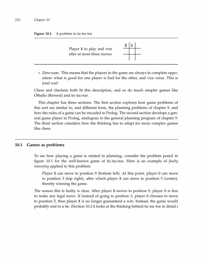
“run” — 2011/9/8 — 18:05 — page 210 — #233�

�

�

�

�

�

�

�

Chapter 10210

Figure 10.1. A problem in tic-tac-toe

Player X to play and winafter at most three moves

X O

Zero-sum. This means that the players in the game are always in complete oppo-sition: what is good for one player is bad for the other, and vice versa. This istotal war!

Chess and checkers both fit this description, and so do much simpler games likeOthello (Reversi) and tic-tac-toe.

This chapter has three sections. The first section explores how game problems ofthis sort are similar to, and different from, the planning problems of chapter 9, andhow the rules of a game can be encoded in Prolog. The second section develops a gen-eral game player in Prolog, analogous to the general planning program of chapter 9.The third section considers how the thinking has to adapt for more complex gameslike chess.

10.1 Games as problems

To see how playing a game is related to planning, consider the problem posed infigure 10.1 for the well-known game of tic-tac-toe. Here is an example of faultyreasoning applied to this problem:

Player X can move to position 9 (bottom left). At this point, player O can moveto position 3 (top right), after which player X can move to position 5 (center),thereby winning the game.

The reason this is faulty is clear. After player X moves to position 9, player O is freeto make any legal move. If instead of going to position 3, player O chooses to moveto position 5, then player X is no longer guaranteed a win. Instead, the game wouldprobably end in a tie. (Section 10.2.4 looks at the thinking behind tic-tac-toe in detail.)

“run” — 2011/9/8 — 18:05 — page 211 — #234�

�

�

�

�

�

�

�

Case Study: Playing Strategic Games 211

10.1.1 How a game can be defined

It is the fact that one player does not control the moves of the other player that makesgames different from planning. Nonetheless, there are some clear similarities. A game(whether very complex like chess or very simple like tic-tac-toe) can be characterizedby the following:

There are two players. One of them moves first.

There is a space of states in the game. One of them is the initial state of the game.There is also a final state of the game, where the game is over and one of the twoplayers is the winner (or there is a tie).

In any state that is not a final state of the game, there is a set of legal moves, thatgo from one game state to another. Throughout the game, players take turnschoosing a move that is legal in the current state.

For any given game, the rules of the game characterize it in these terms. Note that therules of the game always tell how to play the game, but they do not tell how to playit well (see section 10.2).

In the previous chapter, three predicates were used to characterize any planningproblem in Prolog: initial_state, goal_state, and legal_move. It will be similarfor games except that there are four predicates:

player(player). This says that player is one of the two players in the game.

initial_state(state, player). This says that the game starts in state and thatplayer moves first.

game_over(state, player,winner). This says that when it is the turn of player instate, then the game is over and winner wins. The winner is either one of the twoplayers, or the special constant neither when there is a tie.

legal_move(state1, player,move, state2). This says that when it is the turn of playerin state1, then move is legal and the game goes to state2, where it will be the turnof the other player.

These four predicates are used to define each of the games considered in this chapter.

10.1.2 A first example: Race to 21

Race to 21 is an even simpler game than tic-tac-toe:

There are 21 chips on a table. Players take turns removing either one or twochips. The player removing the last chip wins.

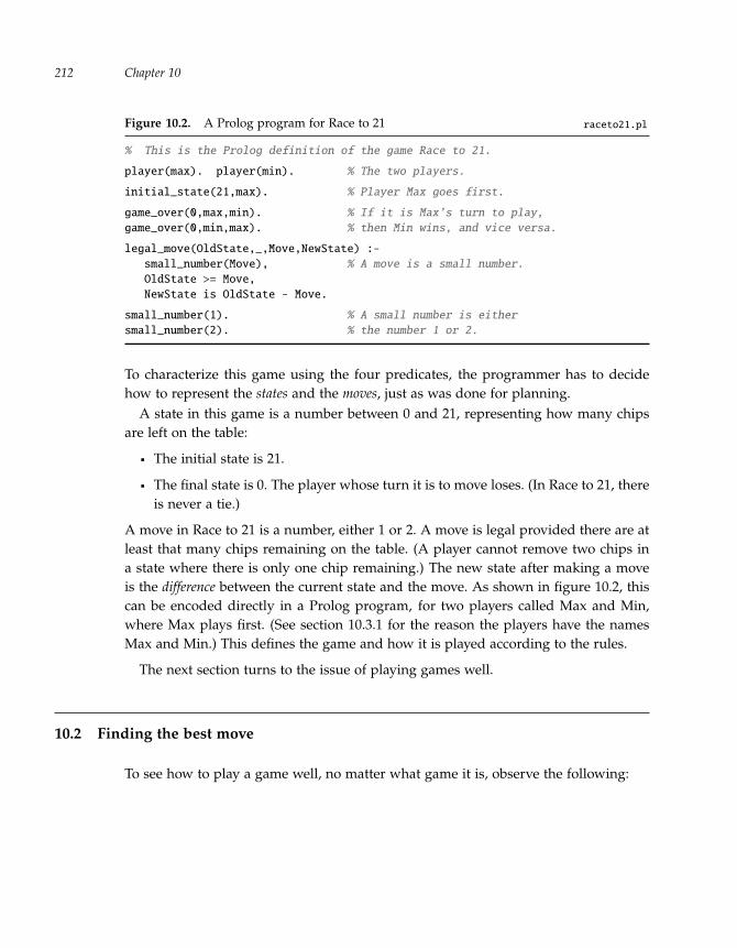
“run” — 2011/9/8 — 18:05 — page 212 — #235�

�

�

�

�

�

�

�

Chapter 10212

Figure 10.2. A Prolog program for Race to 21 raceto21.pl

% This is the Prolog definition of the game Race to 21.

player(max). player(min). % The two players.

initial_state(21,max). % Player Max goes first.

game_over(0,max,min). % If it is Max’s turn to play,

game_over(0,min,max). % then Min wins, and vice versa.

legal_move(OldState,_,Move,NewState) :-

small_number(Move), % A move is a small number.

OldState >= Move,

NewState is OldState - Move.

small_number(1). % A small number is either

small_number(2). % the number 1 or 2.

To characterize this game using the four predicates, the programmer has to decidehow to represent the states and the moves, just as was done for planning.

A state in this game is a number between 0 and 21, representing how many chipsare left on the table:

The initial state is 21.

The final state is 0. The player whose turn it is to move loses. (In Race to 21, thereis never a tie.)

A move in Race to 21 is a number, either 1 or 2. A move is legal provided there are atleast that many chips remaining on the table. (A player cannot remove two chips ina state where there is only one chip remaining.) The new state after making a moveis the difference between the current state and the move. As shown in figure 10.2, thiscan be encoded directly in a Prolog program, for two players called Max and Min,where Max plays first. (See section 10.3.1 for the reason the players have the namesMax and Min.) This defines the game and how it is played according to the rules.

The next section turns to the issue of playing games well.

10.2 Finding the best move

To see how to play a game well, no matter what game it is, observe the following:

“run” — 2011/9/8 — 18:05 — page 213 — #236�

�

�

�

�

�

�

�


A player will not need to find a list of moves from an initial to a final state. Theplayer must find the best next move, wait for the opponent to make a move, thenfind the best next move again, and so on, until the game is over.

The best next move for a player must take into account the responses available tothe opponent. The responses from the opponent will also take into account thepossible counterresponses from the player, which should take into account thepossible counter-counterresponses, and so on.

The best next move for a player should not rely on the opponent’s making amistake. If an opponent plays poorly, so much the better. Ideally, however, a playerwill find a move that is a first step toward winning even when the opponent isplaying at her very best.

10.2.1 Game trees

To see how players can take into account all the possible responses, the counterre-sponses and so on, it is useful to look at a structure called a game tree, whose nodescorrespond to states of the game:

The root node of the tree (usually at the top) is the initial state of the game.

Each leaf node of the tree (usually at the bottom) is a final state of the game,where according to the rules, one of the players has won or there is a tie.

Each non-leaf node has as children (below it) all the game states that can bereached by making legal moves according to the rules.

Figure 10.3 shows a game tree for an anonymous game between two players, Maxand Min. In this game, in the initial state (level 0), Max has two moves available tohim (move 1 and move 2). In the two states to which these moves lead at level 1,Min has three legal moves available to her, leading to six states at level 2. From there,Max has either two or three moves available to him, which either lead to the game’sbeing over at level 3, or Min’s moving one final time from level 3 to level 4. The treedepicts all possible unfoldings of this game, ending with final states where either Maxwins (labeled W) or Min wins (labeled L). The tree does not display what the states orthe moves of the game are. Nonetheless, the rules of the game determine the entirestructure of this game tree, from the start to the end.

The main observation is that just by looking at how the game unfolds according tothe tree, one can determine whether Max should choose move 1 or move 2 as his firstmove. To figure this out, every node on the tree is labeled as either a winning positionfor Max (W) or a winning position for Min (L).

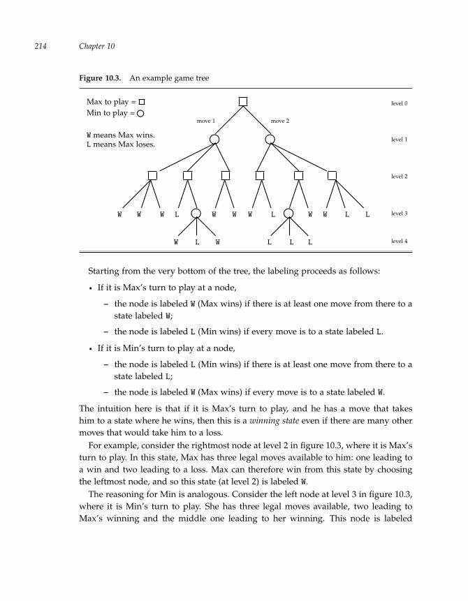
“run” — 2011/9/8 — 18:05 — page 214 — #237�

�

�

�

�

�

�

�

Chapter 10214

Figure 10.3. An example game tree

Max to play =Min to play = �W means Max wins.L means Max loses.

move 1 move 2��

��

��

��

��

��

��

��

��

��

��

��

��

��

��

��

��

��

��

��

��

��

��

��

W W W L W

W W L

W W L L

W L W L L L

level 0

level 1

level 2

level 3

level 4

Starting from the very bottom of the tree, the labeling proceeds as follows:

If it is Max’s turn to play at a node,

– the node is labeled W (Max wins) if there is at least one move from there to astate labeled W;

– the node is labeled L (Min wins) if every move is to a state labeled L.

If it is Min’s turn to play at a node,

– the node is labeled L (Min wins) if there is at least one move from there to astate labeled L;

– the node is labeled W (Max wins) if every move is to a state labeled W.

The intuition here is that if it is Max’s turn to play, and he has a move that takeshim to a state where he wins, then this is a winning state even if there are many othermoves that would take him to a loss.

For example, consider the rightmost node at level 2 in figure 10.3, where it is Max’sturn to play. In this state, Max has three legal moves available to him: one leading toa win and two leading to a loss. Max can therefore win from this state by choosingthe leftmost node, and so this state (at level 2) is labeled W.

The reasoning for Min is analogous. Consider the left node at level 3 in figure 10.3,where it is Min’s turn to play. She has three legal moves available, two leading toMax’s winning and the middle one leading to her winning. This node is labeled

“run” — 2011/9/8 — 18:05 — page 215 — #238�

�

�

�

�

�

�

�


Figure 10.4. A labeled game tree

Max to play =Min to play = �W means Max wins.L means Max loses.

move 1 move 2��

��

��

��

��

��

��

��

��

��

��

��

��

��

��

��

��

��

��

��

��

��

��

��

W W W L W

W W L

W W L L

W L W L L L

W

L

L W

L

W

L

W W

W

W

Max can force a winby making move 2.

L, since by choosing the middle option, Min can guarantee a win. At one level up(level 2), Max has two choices, which are now both labeled L. So Max has no winningmove, and this node is labeled L.

Continuing in this way from the bottom up leads to the labeling shown infigure 10.4. Then two things become clear:

The initial state is a winning state for Max.

The best move for Max to make is move 2, which can lead to a win no matterwhat Min does (and despite all the L labels on the leaves).

So as with planning, the game player can decide on a good first move if the search iscarried ahead all the way to the goal. But unlike with planning, it is not sufficient tofind a single path to the goal; all the possible responses and counterresponses mustbe considered all the way to the end.

10.2.2 A general game player

This process on one example game tree can be generalized to deal with any game,including games with ties. Here is how to label a node for state S in a game betweentwo players P and Q, assuming it is P’s turn to play, as being either a winning positionfor P, a winning position for Q, or neither:

“run” — 2011/9/8 — 18:05 — page 216 — #239�

�

�

�

�

�

�

�

Chapter 10216

Figure 10.5. A general game player gameplayer.pl

% This general game player needs these predicates to be defined:

% - player(Player)

% - game_over(State,Player,Winner)

% - legal_move(BeforeState,Player,Move,AfterState)

% label(S,P,W): state S with player P to move is labeled winner W.

label(S,P,W) :- game_over(S,P,W).

label(S,P,P) :- win_move(S,P,_).

label(S,P,neither) :- \+ win_move(S,P,_), tie_move(S,P,_).

label(S,P,Q) :- opp(P,Q), \+ tie_move(S,P,_), \+ game_over(S,P,_).

% win_move(S,P,M): P can win by making move M.

win_move(S,P,M) :- \+ game_over(S,P,_), opp(P,Q),

legal_move(S,P,M,New), label(New,Q,P).

% tie_move(S,P,M): P can avoid losing by making move M.

tie_move(S,P,M) :- \+ game_over(S,P,_), opp(P,Q),

legal_move(S,P,M,New), \+ label(New,Q,Q).

opp(P,Q) :- player(P), player(Q), \+ P=Q.

1. If the game is over in state S, then label the node with the winner (P, Q, orneither) according to the rules of the game.

2. Otherwise, label the node with P as the winner if there is a legal move from S toa state S′ where S′ is labeled with P as the winner. This move is called a winningmove for P in game state S.

3. Otherwise, label the node with neither as the winner if there is a legal movefrom S to a state S′ where S′ is not labeled with Q as the winner. This move iscalled a nonlosing move for P in game state S.

4. Otherwise, label the node with Q as the winner.

Except for condition 3 (having to do with ties), this summarizes what was donein the tree for Max and Min in figure 10.4. Regarding a tie, a node is labeled withneither when a player has no winning move but has a move to a state that is notlabeled with the opponent’s winning.

These principles can be encoded in a Prolog program, shown in figure 10.5. Thisdefines a general game player. As with planning, for each specific game, a program-mer will need to provide clauses that define the player, game_over, and legal_movepredicates for that game. (The initial_state predicate is not used here.) Once theseare provided, the predicate win_move can be used to see if there is a winning movefrom a state; and tie_move, to see if there is a move that avoids losing.

“run” — 2011/9/8 — 18:05 — page 217 — #240�

�

�

�

�

�

�

�


10.2.3 Playing Race to 21

To see how the general game-playing program works with a specific game like Raceto 21, load both programs into Prolog. To understand how winning moves are found,it is best to start by looking at states very near to the end of a game. For example, inRace to 21, it is clear that if there are only one or two chips left, then the player whoseturn it is to play has a winning move:

?- win_move(1,_,M).

M = 1

?- win_move(2,_,M).

M = 2

Here the move leads directly to a final state where the player is the winner (becausethere are no chips left). It is also evident that if there are three chips left, then there isno winning move:

?- win_move(3,_,M).

No

This is because after any legal move, the game is in a state that is a winner for theopponent. So 3 is a not winning position for the player who has to play. If there arefour or five chips left, then there is a winning move:

?- win_move(5,_,M).

M = 2

?- win_move(4,_,M).

M = 1

The reason that 2 is a winning move for a player with five chips left is that 5 − 2 = 3is not a winning position for the opponent. The case with four chips is similar. Whatabout six chips?

?- win_move(6,max,M).

No

The reason Max does not win with six chips is the following. If he takes one chip,then there are five left for Min, and this would be a winning position (for Min); if hetakes two chips, then there would be four chips left, and this, too, wins for Min. Sothere is nothing Max can do with six chips to guarantee a win.

Similar reasoning would show that 9 is also not a winning position, nor is 12 or 15.In general, for Race to 21, a player cannot guarantee a win if the number of chips left

“run” — 2011/9/8 — 18:05 — page 218 — #241�

�

�

�

�

�

�

�

Chapter 10218

is divisible by 3. In particular, at the start of the game, Max, who moves first, cannotguarantee a win:

?- win_move(21,max,M).

No

Once Max moves, by taking either one or two chips, Min will be able to make awinning move by leaving Max with eighteen chips, that number being divisible by 3:

?- win_move(20,min,M).

M = 2

?- win_move(19,min,M).

M = 1

So the behavior of win_move makes clear that if Min plays perfectly, Max will lose.Observe that this strategy of keeping the number of chips available to the opponentdivisible by 3 is not programmed anywhere. It emerges out of looking at the entiregame tree and labeling each of the nodes.

10.2.4 A second example: Tic-tac-toe

In some way tic-tac-toe is simpler than Race to 21, and playing it well is a challengeonly for very young players. But there are some interesting complications, includingthe possibility of a tie.

The first decision in writing a tic-tac-toe program is how to represent the states andmoves. A state of the 3× 3 board in tic-tac-toe is determined by the markers in each ofthe nine possible positions. So a state can be represented by a list with nine elements,[p1, p2, p3, p4, p5, p6, p7, p8, p9], where each pi is x or o or another character indicatingblank, here a hyphen - (not to be confused the Prolog underscore, _). So the initialstate of a tic-tac-toe game is represented by the list [-,-,-,-,-,-,-,-,-], where allthe positions are vacant. The game is over in any state where one of the followingconditions holds:

There are three x marks making a straight line (x wins).

There are three o marks making a straight line (o wins).

Every pi in the state is either x or o (the board is full).

A move in tic-tac-toe involves a player’s putting a mark in one of the vacant positions.So a move is represented by a number m such that 1 ≤ m ≤ 9, with the proviso thatin the current state, pm = -.

“run” — 2011/9/8 — 18:05 — page 219 — #242�

�

�

�

�

�

�

�


Figure 10.6. A Prolog program for tic-tac-toe tictactoe.pl

player(x). player(o). % This is the tic-tac-toe game.

initial_state([-,-,-,-,-,-,-,-,-],x). % x moves first.

game_over(S,_,Q) :- three_in_row(S,Q). % A winner

game_over(S,_,neither) :- \+ legal_move(S,_,_,_). % A tie

three_in_row([P,P,P,_,_,_,_,_,_],P) :- player(P).

three_in_row([_,_,_,P,P,P,_,_,_],P) :- player(P).

three_in_row([_,_,_,_,_,_,P,P,P],P) :- player(P).

three_in_row([P,_,_,P,_,_,P,_,_],P) :- player(P).

three_in_row([_,P,_,_,P,_,_,P,_],P) :- player(P).

three_in_row([_,_,P,_,_,P,_,_,P],P) :- player(P).

three_in_row([P,_,_,_,P,_,_,_,P],P) :- player(P).

three_in_row([_,_,P,_,P,_,P,_,_],P) :- player(P).

legal_move([-,B,C,D,E,F,G,H,I],P,1,[P,B,C,D,E,F,G,H,I]).

legal_move([A,-,C,D,E,F,G,H,I],P,2,[A,P,C,D,E,F,G,H,I]).

legal_move([A,B,-,D,E,F,G,H,I],P,3,[A,B,P,D,E,F,G,H,I]).

legal_move([A,B,C,-,E,F,G,H,I],P,4,[A,B,C,P,E,F,G,H,I]).

legal_move([A,B,C,D,-,F,G,H,I],P,5,[A,B,C,D,P,F,G,H,I]).

legal_move([A,B,C,D,E,-,G,H,I],P,6,[A,B,C,D,E,P,G,H,I]).

legal_move([A,B,C,D,E,F,-,H,I],P,7,[A,B,C,D,E,F,P,H,I]).

legal_move([A,B,C,D,E,F,G,-,I],P,8,[A,B,C,D,E,F,G,P,I]).

legal_move([A,B,C,D,E,F,G,H,-],P,9,[A,B,C,D,E,F,G,H,P]).

A Prolog program for tic-tac-toe is shown in figure 10.6. As before, the predi-cates player, initial_state, game_over, and legal_move are defined. The predicatethree_in_row is used to check if a player’s mark (either x or o) completes one ofthe three horizontal lines, three vertical lines, or two diagonal lines (and hence theeight clauses). The legal_move predicate has nine clauses, one for each of the possi-ble moves. In each case, it confirms that there is a - in the appropriate position forthe move and replaces the - by the player’s mark in the new state, using variables toleave all the other eight positions unchanged.

If this program is loaded with the general game player, it can show how to make agood move in various states of the game. For example, suppose X first put his mark inposition 1, and then O put hers in position 2. The options X now has are the following:

?- win_move([x,o,-,-,-,-,-,-,-],x,M).

M = 4 ; % A surprising move for X, perhaps

M = 5 ; % The center

M = 7 ; % A corner but not 3 or 9

No

“run” — 2011/9/8 — 18:05 — page 220 — #243�

�

�

�

�

�

�

�

Chapter 10220

Among other things, this shows that player X can choose to move to position 4 andstill be guaranteed a win.

Let us step back one move from this state to see what player O should have donedifferently when X had a single mark on the board:

?- win_move([x,-,-,-,-,-,-,-,-],o,M).

No

?- tie_move([x,-,-,-,-,-,-,-,-],o,M).

M = 5 ;

No

There is nothing O can do to guarantee a win after X chooses position 1. However,there is a move (and only one move) that will be sufficient to ensure that she does notlose, and that is the center square, position 5.

What X should do in the initial state:

?- win_move([-,-,-,-,-,-,-,-,-],x,M).

No

?- tie_move([-,-,-,-,-,-,-,-,-],x,M).

M = 1 ; M = 2 ; M = 3 ; M = 4 ; M = 5 ;

M = 6 ; M = 7 ; M = 8 ; M = 9

As we might already know from actually playing tic-tac-toe, there is nothing that thefirst player can do to guarantee a win at the outset. Not so well known is the fact thatany first move is as good as any other in terms of making sure that the player does notlose. So even with a game as simple as tic-tac-toe, there are perhaps some surprisesthat can be revealed by the game-playing program.

∗ 10.2.5 Playing an entire game

Although this adds nothing to the thinking behind game playing, it is fun to play anentire game from the initial state to a final state rather than just making a single nextbest move. A Prolog program that does this is shown in figure 10.7.

This program will work with the general game player and any game. The mainpredicate here is play_user, and its argument is used to indicate which of the twoplayers in the game will be played by the user (that is, will not be played by thecomputer). So for tic-tac-toe, the query play_user(x) would play a game where theuser is player X (plays first), and play_user(nobody) would play a game where thecomputer plays both sides.

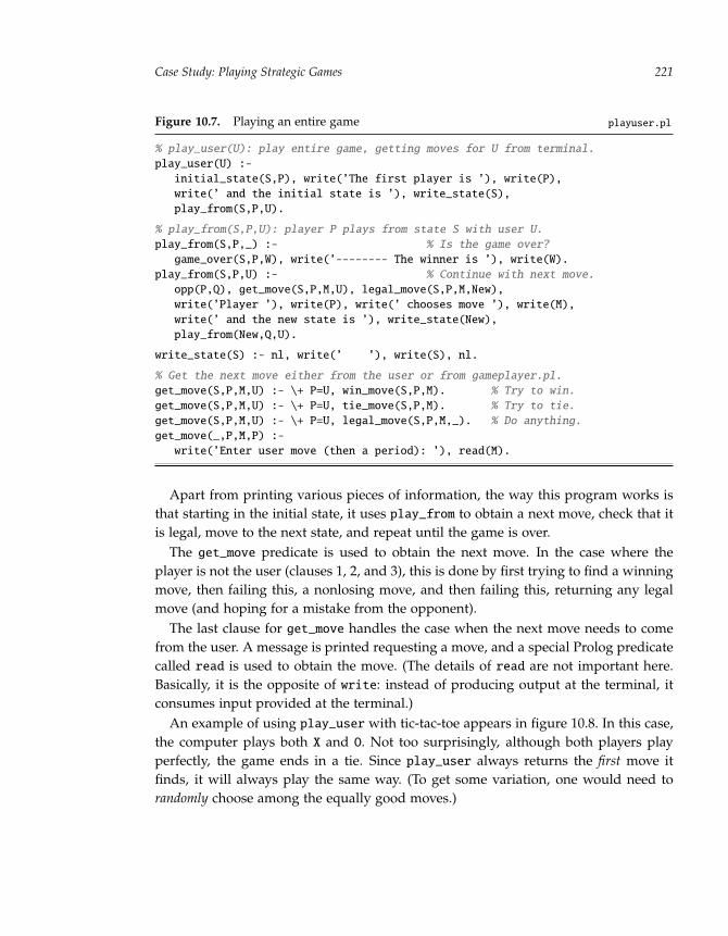
“run” — 2011/9/8 — 18:05 — page 221 — #244�

�

�

�

�

�

�

�


Figure 10.7. Playing an entire game playuser.pl

% play_user(U): play entire game, getting moves for U from terminal.

play_user(U) :-

initial_state(S,P), write(’The first player is ’), write(P),

write(’ and the initial state is ’), write_state(S),

play_from(S,P,U).

% play_from(S,P,U): player P plays from state S with user U.

play_from(S,P,_) :- % Is the game over?

game_over(S,P,W), write(’-------- The winner is ’), write(W).

play_from(S,P,U) :- % Continue with next move.

opp(P,Q), get_move(S,P,M,U), legal_move(S,P,M,New),

write(’Player ’), write(P), write(’ chooses move ’), write(M),

write(’ and the new state is ’), write_state(New),

play_from(New,Q,U).

write_state(S) :- nl, write(’ ’), write(S), nl.

% Get the next move either from the user or from gameplayer.pl.

get_move(S,P,M,U) :- \+ P=U, win_move(S,P,M). % Try to win.

get_move(S,P,M,U) :- \+ P=U, tie_move(S,P,M). % Try to tie.

get_move(S,P,M,U) :- \+ P=U, legal_move(S,P,M,_). % Do anything.

get_move(_,P,M,P) :-

write(’Enter user move (then a period): ’), read(M).

Apart from printing various pieces of information, the way this program works isthat starting in the initial state, it uses play_from to obtain a next move, check that itis legal, move to the next state, and repeat until the game is over.

The get_move predicate is used to obtain the next move. In the case where theplayer is not the user (clauses 1, 2, and 3), this is done by first trying to find a winningmove, then failing this, a nonlosing move, and then failing this, returning any legalmove (and hoping for a mistake from the opponent).

The last clause for get_move handles the case when the next move needs to comefrom the user. A message is printed requesting a move, and a special Prolog predicatecalled read is used to obtain the move. (The details of read are not important here.Basically, it is the opposite of write: instead of producing output at the terminal, itconsumes input provided at the terminal.)

An example of using play_user with tic-tac-toe appears in figure 10.8. In this case,the computer plays both X and O. Not too surprisingly, although both players playperfectly, the game ends in a tie. Since play_user always returns the first move itfinds, it will always play the same way. (To get some variation, one would need torandomly choose among the equally good moves.)

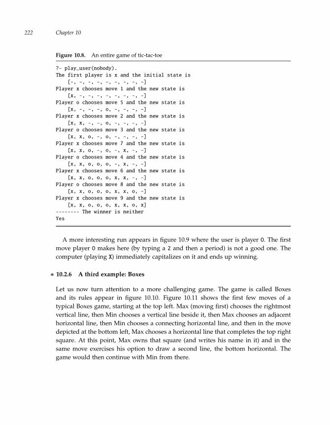
“run” — 2011/9/8 — 18:05 — page 222 — #245�

�

�

�

�

�

�

�

Chapter 10222

Figure 10.8. An entire game of tic-tac-toe

?- play_user(nobody).

The first player is x and the initial state is

[-, -, -, -, -, -, -, -, -]

Player x chooses move 1 and the new state is

[x, -, -, -, -, -, -, -, -]

Player o chooses move 5 and the new state is

[x, -, -, -, o, -, -, -, -]


[x, x, -, -, o, -, -, -, -]


[x, x, o, -, o, -, -, -, -]


[x, x, o, -, o, -, x, -, -]


[x, x, o, o, o, -, x, -, -]


[x, x, o, o, o, x, x, -, -]


[x, x, o, o, o, x, x, o, -]


[x, x, o, o, o, x, x, o, x]

-------- The winner is neither

Yes

A more interesting run appears in figure 10.9 where the user is player O. The firstmove player O makes here (by typing a 2 and then a period) is not a good one. Thecomputer (playing X) immediately capitalizes on it and ends up winning.

∗ 10.2.6 A third example: Boxes

Let us now turn attention to a more challenging game. The game is called Boxesand its rules appear in figure 10.10. Figure 10.11 shows the first few moves of atypical Boxes game, starting at the top left. Max (moving first) chooses the rightmostvertical line, then Min chooses a vertical line beside it, then Max chooses an adjacenthorizontal line, then Min chooses a connecting horizontal line, and then in the movedepicted at the bottom left, Max chooses a horizontal line that completes the top rightsquare. At this point, Max owns that square (and writes his name in it) and in thesame move exercises his option to draw a second line, the bottom horizontal. Thegame would then continue with Min from there.

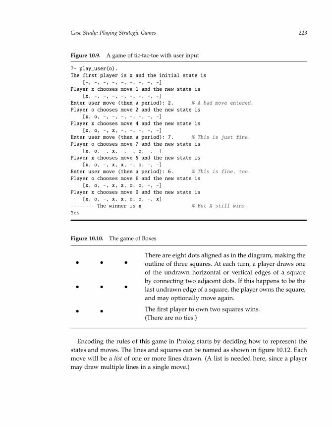
“run” — 2011/9/8 — 18:05 — page 223 — #246�

�

�

�

�

�

�

�


Figure 10.9. A game of tic-tac-toe with user input

?- play_user(o).

The first player is x and the initial state is

[-, -, -, -, -, -, -, -, -]


[x, -, -, -, -, -, -, -, -]

Enter user move (then a period): 2. % A bad move entered.


[x, o, -, -, -, -, -, -, -]


[x, o, -, x, -, -, -, -, -]

Enter user move (then a period): 7. % This is just fine.


[x, o, -, x, -, -, o, -, -]


[x, o, -, x, x, -, o, -, -]

Enter user move (then a period): 6. % This is fine, too.


[x, o, -, x, x, o, o, -, -]


[x, o, -, x, x, o, o, -, x]

-------- The winner is x % But X still wins.

Yes

Figure 10.10. The game of Boxes

�

�

�

�

�

�

�

�There are eight dots aligned as in the diagram, making theoutline of three squares. At each turn, a player draws oneof the undrawn horizontal or vertical edges of a squareby connecting two adjacent dots. If this happens to be thelast undrawn edge of a square, the player owns the square,and may optionally move again.

The first player to own two squares wins.(There are no ties.)

Encoding the rules of this game in Prolog starts by deciding how to represent thestates and moves. The lines and squares can be named as shown in figure 10.12. Eachmove will be a list of one or more lines drawn. (A list is needed here, since a playermay draw multiple lines in a single move.)

“run” — 2011/9/8 — 18:05 — page 224 — #247�

�

�

�

�

�

�

�

Chapter 10224

Figure 10.11. The start of a game of Boxes

�

�

�

�

�

�

�

�

⇒�

�

�

�

�

�

�

�

⇒�

�

�

�

�

�

�

�

⇓

�

�

�

�

�

�

�

�

Max

⇐�

�

�

�

�

�

�

�

⇐�

�

�

�

�

�

�

�

Figure 10.12. Naming the parts of the Boxes board

�

�

�

�

�

�

�

�1 2

3 4 5

6 7

8 9

10

Square 1 has lines 1, 3, 4, 6



As for the states of Boxes, perhaps the simplest thing to do is to think in terms ofsituations and fluents (see section 9.4.1). A state will be a list of terms of the formdraw(player, line), with the most recent drawings first. This allows calculating all thefluents that are needed to decide if a move is legal and when the game is over.

The full specification of the Boxes game in Prolog appears in figure 10.13. Tosummarize briefly how it works, the game is over if a player owns two squares.The successor state clauses for owns say that a player owns a square in a situationif either the player just drew a line that is the last available line for that squareor the player already owned that square in the previous situation. The predicatelast_available_line says that a line is the last one for a square in a situation ifit is available, and nothing is available for that square once the line is drawn. The

“run” — 2011/9/8 — 18:05 — page 225 — #248�

�

�

�

�

�

�

�


Figure 10.13. A Prolog program for Boxes boxes.pl

player(max). player(min). % This is the Boxes game.

square_lines(sq1,[1,3,4,6]). % Lines for square 1



initial_state([],max). % Initially no lines are drawn.

game_over(St,_,W) :- % Winner W owns two squares.

owns(W,Sq1,St), owns(W,Sq2,St), \+ Sq1 = Sq2.

% Player P owns Sq if just drew last line or owned Sq before.

owns(P,Sq,[draw(P,L)|St]) :- last_avail_line(L,Sq,St).

owns(P,Sq,[_|St]) :- owns(P,Sq,St).

% Line L is available and is the last of square not yet drawn.

last_avail_line(L,Sq,St) :-

avail_line(L,Sq,St), \+ avail_line(_,Sq,[draw(_,L)|St]).

% Line L is from Sq and not yet drawn in state St.

avail_line(L,Sq,St) :-

square_lines(Sq,Ls), member(L,Ls), \+ member(draw(_,L),St).

% The legal moves

legal_move(St,P,[L],[draw(P,L)|St]) :- % Draw a line and stop.

avail_line(L,_,St).

legal_move(St,P,[L|Rest],New) :- % Draw a line and go on.

last_avail_line(L,_,St), legal_move([draw(P,L)|St],P,Rest,New).

predicate available_line says that a line is available for a square in a situation ifit is one of the lines for that square, and there is no previous draw action involvingthat line in the situation. Finally, the last two clauses of the program describe when amove is legal: either a list with a single line, or a list with more than one line, when alast available line for a square was just drawn.

Figure 10.14 shows the Boxes game in action:

The first query asks if Max has a winning move from the configuration drawnon the right-hand side. The answer is that Max can win by drawing line 3(completing a square) and then drawing line 8 in the same move.

The second query asks a similar question for the configuration drawn there. Inthis case, Max can win by drawing line 7, but at this point, although he has theoption of continuing with another line, he must not do so. Furthermore, this isthe only winning move.

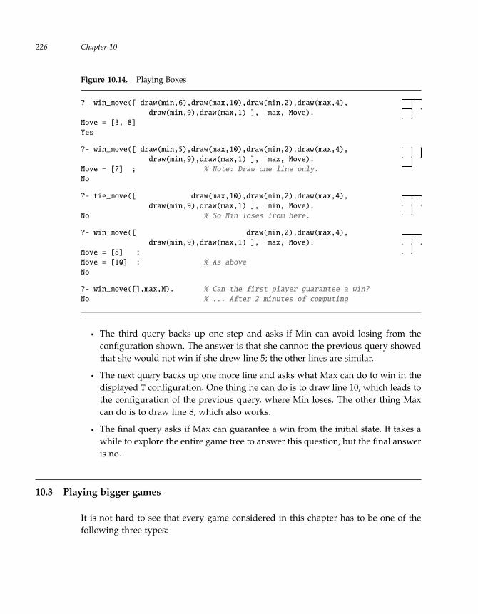
“run” — 2011/9/8 — 18:05 — page 226 — #249�

�

�

�

�

�

�

�

Chapter 10226

Figure 10.14. Playing Boxes

?- win_move([ draw(min,6),draw(max,10),draw(min,2),draw(max,4),

draw(min,9),draw(max,1) ], max, Move).

Move = [3, 8]

Yes

?- win_move([ draw(min,5),draw(max,10),draw(min,2),draw(max,4),


Move = [7] ; % Note: Draw one line only.

No

?- tie_move([ draw(max,10),draw(min,2),draw(max,4),

draw(min,9),draw(max,1) ], min, Move).

No % So Min loses from here.

?- win_move([ draw(min,2),draw(max,4),


Move = [8] ;

Move = [10] ; % As above

No

?- win_move([],max,M). % Can the first player guarantee a win?

No % ... After 2 minutes of computing

��

��

��

��

��

��

��

��

The third query backs up one step and asks if Min can avoid losing from theconfiguration shown. The answer is that she cannot: the previous query showedthat she would not win if she drew line 5; the other lines are similar.

The next query backs up one more line and asks what Max can do to win in thedisplayed T configuration. One thing he can do is to draw line 10, which leads tothe configuration of the previous query, where Min loses. The other thing Maxcan do is to draw line 8, which also works.

The final query asks if Max can guarantee a win from the initial state. It takes awhile to explore the entire game tree to answer this question, but the final answeris no.

10.3 Playing bigger games

It is not hard to see that every game considered in this chapter has to be one of thefollowing three types:

“run” — 2011/9/8 — 18:05 — page 227 — #250�

�

�

�

�

�

�

�


a game where both players can force a tie or better (as in tic-tac-toe);

a game where the player who plays second can force a win (as in Boxes or Raceto 21);

a game where the player who plays first can force a win (none considered).

What does this mean? For a game of type 1, if your opponent does not make amistake, you will not win no matter what you do. For a game of type 2, if you playfirst and your opponent does not make a mistake, you will not win no matter whatyou do. For a game of type 3, if you play second and your opponent does not make amistake, you will not win no matter what you do.

So why should you even bother to play games like these? You could simply do thefollowing:

?- initial_state(S,P), win_move(S,P,Move).

This would tell you, once and for all, what a proper first move should be. Then youcould find a proper second move, and so on. Where is the fun in playing?

The answer is that for sufficiently complex games, it cannot be determined whatthe best first move is once and for all because the game trees are too large to explorefully:

For checkers, the game tree is estimated to have 1070 nodes.

For chess, the game tree is estimated to have 10120 nodes.

For Go, the game tree is estimated to have 10750 nodes.

So the win_move predicate as written here is practical only for very small games. Forbig games, finding a best move must be possible without examining the entire gametree. This is why playing a game like chess remains challenging, and why it is still notknown whether white (who plays first) can guarantee a win. (In 2007 checkers wassolved by Jonathan Schaeffer and his team. It is a type 1 game like tic-tac-toe: bothplayers can avoid losing.)

10.3.1 Numerical game trees and minimax

This section considers a second general game player, one that can decide on a bestmove without looking at the entire game tree. For this purpose, it is useful to imaginea numerical game tree similar to the one in figure 10.3 except that numbers are put onthe leaves of the tree.

From now on, the two game players will always be called Max and Min, and abig positive number (say, 999) indicates that Max wins the game, and a big negative

“run” — 2011/9/8 — 18:05 — page 228 — #251�

�

�

�

�

�

�

�

Chapter 10228

Figure 10.15. An example numeric game tree

move 1 move 2��

��

��

��

��

��

��

��

��

��

��

��

��

��

��

��

��

��

��

8 7 -1 -2 5

9 1 -12

-10 2 -5 3

number (say, −999) indicates that Min wins the game. The number 0 is used when thegame ends in a tie. (So big numbers are good for Max, and small numbers are goodfor Min.)

It is then a simple process to assign a numeric value to every node on the tree.Starting from the bottom of the tree, proceed as follows:

If it is Max’s turn to play, label the node with the maximum of the labels of thechildren of the node.

If it is Min’s turn to play, label the node with the minimum of the labels of thechildren of the node.

This labeling duplicates what was done previously with W and L (and also handlesties properly): a node labeled 999 is a winning position for Max; a node labeled −999is a winning position for Min; and a 0 is neither. Overall because of the minimumsand maximums, this numeric process is called minimax. (This finally also explainswhy Max and Min have the names they do.)

What makes this process interesting is that a numeric game tree need not go all theway to the end of the game but can stop at a certain depth, after which an estimate ismade about the value of the state. A bigger number means that the state is estimatedto be better for Max; a smaller number means that the state is estimated to be betterfor Min. (How to arrive at these estimates is discussed later.)

A tree of this type is shown in figure 10.15. The tree stops at depth 3, and estimatedvalues are provided for all the leaf nodes. For example, according to this estimate, theleftmost state at level 3 (with a value of 8) is estimated to be slightly better for Max

“run” — 2011/9/8 — 18:05 — page 229 — #252�

�

�

�

�

�

�

�


Figure 10.16. A labeled numeric game tree

move 1 move 2��

��

��

��

��

��

��

��

��

��

��

��

��

��

��

��

��

��

��

8 7 -1 -2 5

9 1 -12

-10 2 -5 3

8 -1 9

-1

1 2 3

1

1

Max can guaranteea value of 1.

(worse for Min) than the state beside it (with a value of 7). In other words, if Max hadto choose, he should choose to move to the leftmost state.

Applying the minimax procedure to this truncated tree results in a label for everynode, as shown in figure 10.16. Max’s best move here according to all the estimates ismove 2, where he will be guaranteed a value of 1 or better no matter what Min does.

But why not simply truncate the tree at depth 1 and use the estimates from thereinstead of going to depth 3? The answer is that the estimates are expected to be moreaccurate, the closer the depth is to the end of the game. An estimate at level 1 may bemuch less useful than the values obtained by minimax with estimates at deeper levels.So there is a trade-off: the deeper the search using estimates, the more accurate theresults will be, but the more nodes have to be considered to decide on a best move. Infact, as with planning (see section 9.3), the number of nodes to be considered growsexponentially with the depth of the tree.

∗ A version of minimax in Prolog

There are many ways to encode the minimax procedure in Prolog, but the easiest isto assume a number v and find a move (if one exists) that guarantees a value of vor better (that is, bigger for Max and smaller for Min). The property to be used in aprogram is that Max can guarantee a value of v or higher if he can move to a statewhere Min cannot guarantee a value of v − 1 or lower. Similarly, Min can guarantee avalue of v or lower if she can move to a state where Max cannot guarantee a value ofv + 1 or higher.

“run” — 2011/9/8 — 18:05 — page 230 — #253�

�

�

�

�

�

�

�

Chapter 10230

Figure 10.17. A minimax procedure in Prolog minimax.pl

% Computing the values of moves for two players, Max and Min.

% The game-dependent predicate estval estimates values of states.

% The search of the game tree is limited to a depth given by D.

% can_get(S,P,D,V): P can get a value of V or better in state S.

can_get(S,max,_,V) :- game_over(S,max,W), winval(W,V1), V1 >= V.

can_get(S,min,_,V) :- game_over(S,min,W), winval(W,V1), V1 =< V.

can_get(S,max,0,V) :- \+ game_over(S,_,_), estval(S,max,E), E >= V.

can_get(S,min,0,V) :- \+ game_over(S,_,_), estval(S,min,E), E =< V.

can_get(S,P,D,V) :- \+ game_over(S,_,_), val_move(S,P,D,_,V).

% val_move(S,P,D,M,V): P can get a value of V or better with move M.

val_move(S,max,D,M,V) :- D>0, D1 is D-1, V1 is V-1,

legal_move(S,max,M,S1), \+ can_get(S1,min,D1,V1).

val_move(S,min,D,M,V) :- D>0, D1 is D-1, V1 is V+1,

legal_move(S,min,M,S1), \+ can_get(S1,max,D1,V1).

winval(max,999). % The value of a state where Max has won

winval(min,-999). % The value of a state where Max has lost

winval(neither,0). % The value of a state with a tie

These ideas lead to the Prolog program shown in figure 10.17. The labeling predi-cate is called can_get. What can_get says for Max (and analogously for Min) is thatMax can get a value of v or better if one of the following conditions holds:

The game is over, and the final value v′ according to the winner (as specified bythe predicate winval) satisfies v′ ≥ v.

The depth d = 0, and the estimated value of the state v′ according to the game-specific predicate estval satisfies v′ ≥ v.

The game is not over, and Max can get a value of v or better by making a move(as specified by the predicate val_move).

The predicate val_move is used for choosing a move. What it says for Max (andanalogously for Min) is that assuming a depth d > 0, Max can guarantee a value of vor better if there is a legal move to a state where Min cannot get a value of v − 1 orbetter (for her) at depth d − 1.

The predicate val_move replaces win_move and tie_move as a general game-playingprogram. If the depth is very large, one will never hit the estimates, and so thevalues will be completely determined by the winner at the end of the game. So thequery val_move(S,max,10000,M,999) asks for a move M for player Max in state Sthat will guarantee a win for Max, as win_move(S,max,M) did before. The query

“run” — 2011/9/8 — 18:05 — page 231 — #254�

�

�

�

�

�

�

�


Figure 10.18. Cutoffs in a game tree

B5

...

A

C E

3

...

D

cutoff

......

...

...

B CE

4

8...

...

A

D

cutoff

...

val_move(S,max,10000,M,0) asks for a move M for player Max in state S that willguarantee at least a tie. When the depth is smaller, and estimates of values have to beused (as provided by the estval predicate), then the guarantees are only relative tothose estimated values.

10.3.2 Alpha and beta cutoffs

Minimax with estimates allows making decisions about how to move in a game with-out searching all the way to the end of the game. But because the search should beas deep as possible for the sake of accuracy, there may still be a very large number ofnodes to consider in a game tree. However, sometimes it is not necessary to look atall those nodes to make the final decision.

Consider the portion of a game tree depicted on the left side in figure 10.18. Thegoal is to assign a value to the node labeled A, where it is Max’s turn to play. To dothis, values must be assigned to the nodes below A, where it is Min’s turn to play. (Maxwill eventually chose the maximum of the values for B, C, E, and any other childrenof A.) Proceeding from left to right as usual, it has already been determined that thevalue of the node labeled B is 5. To get a value for the next node, C, the values of itschildren must be found. (Min will eventually chose the minimum of these values.) Aspart of this process, it has just been determined that the value of node D is 3.

Before continuing with the remaining children of C, observe the following. Thevalue assigned to node C cannot be larger than 3, since Min chooses a minimum.However, whatever the value of C is, it will not change the value for A, since Maxchooses a maximum, and the value of B is already larger than 3. The conclusion is

“run” — 2011/9/8 — 18:05 — page 232 — #255�

�

�

�

�

�

�

�

Chapter 10232

that the search does not have to continue below C, since it cannot affect the result.Therefore perform an alpha cutoff , and jump immediately to node E, which may turnout to affect the value at A.

An analogous situation holds on the right of figure 10.18. In this case, the search isfor a value for A, a node for Min. After it has been determined that B has value 4 andD has value 8, it is clear that C cannot get a value smaller than 8, since Max chooses amaximum. Since Min chooses a minimum at A, and the value of B is already smallerthan 8, perform a beta cutoff , and jump immediately to node E, which may still affectthe value at A.

The alpha and beta cutoffs allow deciding what moves to make (for Max or forMin) without examining an entire tree all the way to the leaves. These cutoffs can bevery significant, especially if they happen high up in the game tree.

10.3.3 The application to chess

A minimax game player is able to decide on a best next move without looking atall the game states up to the end of the game. To use it, however, one needs to beable to estimate the values of states where the game is not over. (This is not unlikeestimating the distance to the goal during planning in section 9.3.2.) So in addition tothe four predicates player, initial_state, legal_move, and game_over, a fifth oneis needed:

estval(state, player, v)

This says that if it is the turn of player in state, then the number v is the estimatedmeasure of how good the state is, from the point of view of Max.

Different games have different methods of estimating how well or how poorly Maxis doing at nonfinal states of the game. For a game like chess, a typical estimate issomething like (material advantage + positional advantage). The material advantage is ofthe form 9 · Q + 5 · R + 3 · N + 3 · B + P, where Q, R, N, B, and P represent theadvantage in queens, rooks, knights, bishops, and pawns, respectively. The positionaladvantage is much harder to quantify but usually includes things like mobility, controlover squares, early development of pieces, and so on.

How well does this work for chess? Although chess-playing programs have existedfor a long time, the first one to win against a world chess champion was Deep Blue,which won against Garry Kasparov in 1997. Here are some details on it:

It used minimax with alpha-beta cutoffs, but on a special computer to speed upthe generation of moves and the evaluation of states. (It was able to consider astaggering 200 million board positions per second.)

“run” — 2011/9/8 — 18:05 — page 233 — #256�

�

�

�

�

�

�

�


Figure 10.19. Chess rating and search depth

4 8 12 14

500

1500

2500

depth of search

rating

. . . . . . . . . . . . . . . . . . . . . . . . . . . . ?

It explored game trees to about depth 14, with occasional very deep searches.The estimates of the values of game states used 8,000 separate factors.

It had a U.S. Chess Federation rating of 2650 in 1996; the rating of a chess grand-master is 2500. (For comparison, the world chess champion as of January 2011,Magnus Carlsen, had a rating of 2814.)

What is perhaps most interesting about the effort in computer chess is that almostnone of it is specific to chess. Instead, it is mostly directed toward speeding up thegame tree search. This is not too surprising, since the U.S. Chess Federation rating ofchess programs seems to be directly proportional to the search depth, as illustratedvery roughly in figure 10.19. (It is worth noting, however, that this effort on searchhas not helped so far with extremely large games like the game of Go.)

Want to read more?

This chapter looked at the thinking behind playing strategic games. Getting comput-ers to play these games, and especially chess, has been a mainstay of AI researchfrom the very beginning. Alan Turing, the father of computer science, tried his handat it, and one of the first minimax chess programs was due to Claude Shannon, thefather of information theory. John McCarthy discovered alpha-beta cutoffs in 1956.

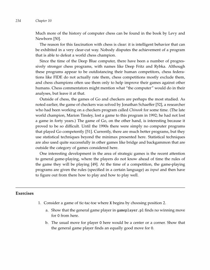
“run” — 2011/9/8 — 18:05 — page 234 — #257�

�

�

�

�

�

�

�

Chapter 10234

Much more of the history of computer chess can be found in the book by Levy andNewborn [50].

The reason for this fascination with chess is clear: it is intelligent behavior that canbe exhibited in a very clear-cut way. Nobody disputes the achievement of a programthat is able to defeat a world chess champion.

Since the time of the Deep Blue computer, there have been a number of progres-sively stronger chess programs, with names like Deep Fritz and Rybka. Althoughthese programs appear to be outdistancing their human competitors, chess federa-tions like FIDE do not actually rate them, chess competitions mostly exclude them,and chess champions often use them only to help improve their games against otherhumans. Chess commentators might mention what “the computer” would do in theiranalyses, but leave it at that.

Outside of chess, the games of Go and checkers are perhaps the most studied. Asnoted earlier, the game of checkers was solved by Jonathan Schaeffer [52], a researcherwho had been working on a checkers program called Chinook for some time. (The lateworld champion, Marion Tinsley, lost a game to this program in 1992; he had not losta game in forty years.) The game of Go, on the other hand, is interesting because itproved to be so difficult. Until the 1990s there were simply no computer programsthat played Go competently [51]. Currently, there are much better programs, but theyuse statistical techniques beyond the minimax presented here. Statistical techniquesare also used quite successfully in other games like bridge and backgammon that areoutside the category of games considered here.

One interesting development in the area of strategic games is the recent attentionto general game-playing, where the players do not know ahead of time the rules ofthe game they will be playing [49]. At the time of a competition, the game-playingprograms are given the rules (specified in a certain language) as input and then haveto figure out from there how to play and how to play well.

Exercises

1. Consider a game of tic-tac-toe where X begins by choosing position 2.

a. Show that the general game player in gameplayer.pl finds no winning movefor O from here.

b. The usual move for player O here would be a center or a corner. Show thatthe general game player finds an equally good move for O.

“run” — 2011/9/8 — 18:05 — page 235 — #258�

�

�

�

�

�

�

�


Figure 10.20. A simple game tree

T WW L L L WL T L TWL WW

2. Consider the game tree depicted in figure 10.20. What is the move that Maxshould make from the root node? Answer by labeling every state of the gametree with W, L, or T (for a tie).

3. This question concerns the intuitive understanding of the labels on a game tree.Suppose players P and Q are playing a game, and each state of the game islabeled with P or Q (as the eventual winner) or neither for a tie.

a. If a state is labeled with P as the winner, which of the following statementsare true?

(1) Throughout the game, no matter what either player does, P willeventually win.

(2) Throughout the game, no matter what Q does, P will be able to choosea move that will eventually lead to a win.

(3) Throughout the game, no matter what P does, Q will be unable to choosea move that will eventually lead to a win (for Q).

b. If a state is labeled with neither as winner, which of the followingstatements are true?

(1) Throughout the game, no matter what either player does, the game willeventually end in a tie.

(2) Throughout the game, no matter what Q does, P will be able to choosea move that will eventually lead to a tie.

(3) Throughout the game, no matter what Q does, P will be able to choosea move that will eventually lead to a tie or a win.

“run” — 2011/9/8 — 18:05 — page 236 — #259�

�

�

�

�

�

�

�

Chapter 10236

Figure 10.21. A numeric game tree

4. One of the reasons the Prolog general game player presented in the filegameplayer.pl may be hard to follow is because of the possibility of a tie. Writea simpler version of label and win_move (and any other predicate you need) forgames where there is always a winner. Show that your program works properlyon Race to 21.

5. Consider the numeric game tree to depth 4 in figure 10.21.

a. Determine the numeric values for all the nodes in the tree.

b. Indicate on the tree where alpha and beta cutoffs would occur, assumingthat the tree is explored in the usual way, from left to right. Of the entiretree, how many leaf nodes do not need to be examined by using alpha-betacutoffs?

6. Consider the following game, called Wythoff’s Nim, a variant of Race to 21:

When the game begins, there is a pile of green chips and a pile of red chipson the table. Each player takes turns removing at least one chip from thetable, and the last player to take a chip wins. In a move, a player may takeany number of green chips, or any number of red chips, or exactly the samenumber of green and red chips.

To encode this game in Prolog, a game state can be represented using a list oftwo numbers [p1, p2], where p1 ≥ 0 is the number of green chips, and p2 ≥ 0 isthe number of red chips. The moves of the game can then be represented by oneof the following terms:

green(m), where 1 ≤ m ≤ p1, when m green chips are to be removed

red(m), where 1 ≤ m ≤ p2, when m red chips are to be removed

“run” — 2011/9/8 — 18:05 — page 237 — #260�

�

�

�

�

�

�

�


both(m), where 1 ≤ m ≤ p1 and 1 ≤ m ≤ p2, indicating that m green chipsand m red chips are to be removed

For example, starting in state [4, 2], here are all of the states that can be reachedin one move: [3, 2], [2, 2], [1, 2], [0, 2], [4, 1], [4, 0], [3, 1], and [2, 0].

To generate legal moves for this game in Prolog, it is useful to be able togenerate numbers between two bounds. You may use the built-in predicatebetween(x, y, z), which holds when x ≤ z ≤ y, and which can generate a zgiven an x and y.

a. Write Prolog clauses defining this game for two players, Max and Min.The initial state is unspecified, so you need to write clauses for player,game_over, and legal_move (using between).

b. Suppose the game is in state [3, 1], where it is Max’s turn to play. Draw thefull game tree (with W and L at the leaves) starting at this state. Use the treeto determine the best next move for Max. Explain your reasoning. Show thatyour program selects this move.

c. Show by running your program that the best move, starting in state [4, 6], isto take one chip from each pile.

d. Consider a sequence of game states defined by the following rule:

The 0th element of the sequence is the state [0, 0];

For any i > 0, the ith element of the sequence is the state [p1, p2], wherep1 is the smallest number that does not appear in an earlier state of thesequence, and where p2 = p1 + i.

Use your program to explore what happens if the initial state of a game isone of the states in this sequence.

7. Use exercise 6d to describe a winning strategy for Wythoff’s Nim. Given anarbitrary state of the game [p1, p2], what is the best move to make?

8. Look on the Internet to discover the strange connection between winning strate-gies for Wythoff’s Nim and the golden mean, that is, (−1+

√5)/2, the remarkable

number studied since the time of the ancient Greeks.

9. The game player presented in the file minimax.pl can find a move to guarantee agiven numeric value, if one exists. However, it cannot find the best move to make,since it does not compare the values produced by all possible moves. Write agame player that does this. Hint: Use the built-in Prolog predicate findall toproduce a list of all the legal moves from some state.

“run” — 2011/9/8 — 18:05 — page 238 — #261�

�

�

�

�

�

�

�

“run” — 2011/9/8 — 18:05 — page 239 — #262�

�

�

�

�

�

�

�

∗ 11 Case Study: Other Ways of Thinking

The discussion in previous chapters demonstrated how thinking supports intelligentbehavior in a variety of domains, including puzzles, visual scenes, English sentences,actions, and games. Thinking uses what is known, and across the domains, the knowl-edge varied, but the thinking procedure was always the same: back-chaining. Evenwith complex extensions, like situations and fluents or minimax, the thinking proce-dure remained the same. This chapter, however, considers other ways of thinking, thatis to say, other ways of using what is known.

These new modes of thinking can be illustrated with a simple example. Considerthe following four sentences:

1. If X is a polar bear, then X is white.

2. Thornton is a polar bear.

3. Thornton is white.

4. If X is a swan, then X is white.

From (1) and (2), the sort of thinking considered so far would allow (3) to be con-cluded, which is a logical entailment of (1) and (2). This sort of reasoning is oftencalled deduction: from (1) and (2), one can deduce (3).

But suppose only (1) and (4) are known. Nothing at all is known about the indi-vidual, Thornton. If he were actually observed to be white, one might conjecture thathe is a polar bear, since it is known that polar bears are white. This sort of thinkingis not deductive; it does not come with the guarantee of logical entailment. Thorntonmight be a swan or something completely different. Nonetheless, the conjecture thatThornton is a polar bear accounts for the color, as does the conjecture that he is aswan. This type of nondeductive thinking was called abduction by the philosopherC. S. Peirce: from (1) and (3), one can abduce (2). This is the sort of reasoning thatunderlies explanation: according is what is known, Thornton being a polar bear wouldexplain his being white.

Now assume that at first only (2) and (3) are known. Nothing at all is known aboutthe color of polar bears or of swans. But then imagine (5) and (6) are observed:

“run” — 2011/9/8 — 18:05 — page 240 — #263�

�

�

�

�

�

�

�

Chapter 11240

5. Shako is a polar bear, and Shako is white.

6. Peppy is a polar bear, and Peppy is white.

One might want to generalize from these and surmise that all polar bears are white.Again, this sort of thinking is not deductive. The facts about the individuals do notlogically entail that all polar bears are white; the very next polar bear could turn outto be a different color. C. S. Peirce called this type of nondeductive thinking induction:from (2) and (3) (and others like it), one can induce (1). This is the sort of reasoningthat underlies a form of learning: from observing the color of polar bears Thornton,Shako, Peppy, and perhaps others, one learns that as a rule, polar bears are white.

So, to summarize:from (1) and (2), one can deduce (3);

from (1) and (3), one can abduce (2);

from (2) and (3), one can induce (1).

Finally, suppose (7) is added:

7. Freddy is a either a polar bear or a swan.

Based on what is known, one can conclude (that is, deduce) that Freddy is white. Thisis logically entailed by (1), (4), and (7). If (7) is true, then there are only two possi-bilities, and in either case, given (1) and (4), the color must be white. However, thisconclusion could not be drawn using the current thinking procedure, back-chaining.There is no way to even represent a sentence like (7), since it is neither an atomicsentence nor a conditional. This chapter also explores what is involved with thissort of thinking, called propositional reasoning. (It is sometimes also known as Booleanreasoning.) Back-chaining is a special case.

The chapter is divided into four sections. The first section reexamines back-chainingas the starting point for discussing the other ways of thinking. Sections 2, 3, and 4discuss explanation, learning, and propositional reasoning, respectively.

There is something of a paradox in using Prolog and back-chaining to look atnew ways of thinking that go beyond back-chaining. And as the paradox is resolved,thinking itself will end up becoming the subject matter of the thinking. This reinterpre-tation will require a major conceptual shift, and this chapter is the most technicallychallenging one in the book.

“run” — 2011/9/8 — 18:05 — page 241 — #264�

�

�

�

�

�

�

�

Case Study: Other Ways of Thinking 241

Figure 11.1. A recap of back-chaining

There is a knowledge base of clauses, where each clause has a head, which is an atom,and a body, which is a sequence of atoms. There is also a query, which is a sequenceof atoms. The task is to establish the query given the knowledge base.

The query A1, . . . , An returns success or failure by back-chaining as follows:

1. If n = 0, the query returns success.

2. Otherwise, the query returns success only if there is a clause in the knowledgebase whose head is A1 (the first atom of the query) and whose body is B1, . . . , Bm,such that the query B1, . . . , Bm, A2, . . . , An returns success (recursively) .

11.1 Back-chaining as subject matter

The back-chaining procedure that Prolog uses is summarized in figure 11.1. (This sim-plified version omits negation, equality, and any mention of variables or unificationin the atoms.) In talking about back-chaining, it is assumed that any knowledge to beapplied in thinking is represented symbolically in the knowledge base (KB). The KBcan be about a world of family relationships, or a visual scene, or a game; the clausesin the KB will talk about these items and the relationships among them. An exampleis the clause in the family program in figure 3.1 that relates the father predicate tothe child and male predicates.

But suppose one wants to think about back-chaining itself rather than about fathersand families. The clauses in the KB would have to talk not about people but aboutknowledge bases, clauses and queries. Instead of a predicate like father(x, y) thatholds if person x is a father of person y, there might be a predicate like est(k, q)(short for establish) that holds when the query q can be established by back-chainingfrom the knowledge base k. The arguments to the predicate est would be Prologterms standing for a knowledge base and a query. In sum, clauses, knowledge bases,and queries would be represented as Prolog terms so that they can then be used asarguments to predicates like est.

How is this done? To simplify matters, assume for now that predicates have noarguments. Then a clause can be represented as a Prolog term using a list of constants:the head of the list will represent the head of the clause, and the tail will representthe body of the clause.

“run” — 2011/9/8 — 18:05 — page 242 — #265�

�

�

�

�

�

�

�

Chapter 11242

Consider, for example, the Prolog clause

u :- p, b.

This can be represented by the Prolog term [u,p,b]. Similarly, a knowledge base canbe represented as a list whose elements represent the clauses. Consider, for example,the following simple Prolog knowledge base:

a.

b.

u :- p, b.

p :- a.

This knowledge base can be represented using the following Prolog term:

[ [a], [b], [u,p,b], [p,a] ].

Of course, this list is not a knowledge base itself, but it can be used to represent oneas a Prolog term. Each element of this list is a nonempty list representing a clause.(Atomic clauses are represented as lists with a single element.) Similarly, a query isrepresented as a list of atoms.

With these list representations, there are now sentences in Prolog that talk aboutthe properties of knowledge bases and queries, just as previous sentences talkedabout properties of people. In particular, the predicate est(k, q) should hold if thequery represented by q can be established by back-chaining from the knowledge baserepresented by k. In other words, the following behavior is desired:

?- est([[a],[b],[u,p,b],[p,a]], [p,b]).

Yes

?- est([[a],[b],[u,p,b],[p,a]], [c]).

No

The first query should succeed because the knowledge base represented by the firstargument (that is, the four clauses just listed) logically entails both p and b, the queryrepresented by the second argument. The second query should fail because that sameknowledge base does not logically entail c.

How should this est predicate be defined? Keeping in mind that one is workingnot with knowledge bases and queries but with symbolic representations of them aslists, one can encode what was said about back-chaining in figure 11.1:

The predicate est(k, q) holds if one of the following holds:

1. q is the empty list (where k can be anything).

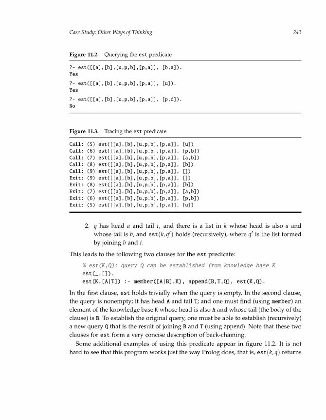
“run” — 2011/9/8 — 18:05 — page 243 — #266�

�

�

�

�

�

�

�


Figure 11.2. Querying the est predicate

?- est([[a],[b],[u,p,b],[p,a]], [b,a]).

Yes

?- est([[a],[b],[u,p,b],[p,a]], [u]).

Yes

?- est([[a],[b],[u,p,b],[p,a]], [p,d]).

No

Figure 11.3. Tracing the est predicate

Call: (5) est([[a],[b],[u,p,b],[p,a]], [u])

Call: (6) est([[a],[b],[u,p,b],[p,a]], [p,b])

Call: (7) est([[a],[b],[u,p,b],[p,a]], [a,b])

Call: (8) est([[a],[b],[u,p,b],[p,a]], [b])

Call: (9) est([[a],[b],[u,p,b],[p,a]], [])

Exit: (9) est([[a],[b],[u,p,b],[p,a]], [])

Exit: (8) est([[a],[b],[u,p,b],[p,a]], [b])

Exit: (7) est([[a],[b],[u,p,b],[p,a]], [a,b])

Exit: (6) est([[a],[b],[u,p,b],[p,a]], [p,b])

Exit: (5) est([[a],[b],[u,p,b],[p,a]], [u])

2. q has head a and tail t, and there is a list in k whose head is also a andwhose tail is b, and est(k, q′) holds (recursively), where q′ is the list formedby joining b and t.

This leads to the following two clauses for the est predicate:

% est(K,Q): query Q can be established from knowledge base K

est(_,[]).

est(K,[A|T]) :- member([A|B],K), append(B,T,Q), est(K,Q).

In the first clause, est holds trivially when the query is empty. In the second clause,the query is nonempty; it has head A and tail T; and one must find (using member) anelement of the knowledge base K whose head is also A and whose tail (the body of theclause) is B. To establish the original query, one must be able to establish (recursively)a new query Q that is the result of joining B and T (using append). Note that these twoclauses for est form a very concise description of back-chaining.

Some additional examples of using this predicate appear in figure 11.2. It is nothard to see that this program works just the way Prolog does, that is, est(k, q) returns

‘‘run’’ --- 2011/9/8 --- 18:05 --- page 244 --- #267�

�

�

�

�

�

�

�

Chapter 11244

success when the query represented by q would return success in Prolog for the knowl-edge base represented by k. The partial trace in figure 11.3 shows that est does itswork in the same order as Prolog’s back-chaining would.

But so what? What is the point of all this? It shows that Prolog is well-suited fordescribing, among other things, how Prolog works. Once one can talk about thinkingthe way that Prolog does, one can also talk about thinking in other ways. So Prolog canbe used to express other thinking procedures that work quite differently from Prologitself. Understanding what those two simple clauses for the predicate est do and whyis crucial to understanding the rest of this chapter.

11.1.1 A breadth-first thinking procedure

Let us examine a thinking procedure that differs from Prolog in a very minor way.Perhaps the simplest part of back-chaining to modify is the order in which atoms

are considered in a query. Consider a partial trace of a query that eventually fails:

Call: (10) est([[a],[b],[u,p,b],[p,a]], [u,c])

Call: (11) est([[a],[b],[u,p,b],[p,a]], [p,b,c])

Call: (12) est([[a],[b],[u,p,b],[p,a]], [a,b,c])

Call: (13) est([[a],[b],[u,p,b],[p,a]], [b,c])

Call: (14) est([[a],[b],[u,p,b],[p,a]], [c])

Fail: (14) est([[a],[b],[u,p,b],[p,a]], [c])

Note that before est can get to the atom c, it has to first deal with u. To deal with u,it has to go deeper and deal with p and b. To deal with p, it has to go deeper still anddeal with a. Once it is done with a, it can go on to b. Once it is done with b, it finallygets to c, and then the query fails.

This sort of procedure is called a depth-first procedure, since the program handlesnew atomic queries that arise from the bodies of clauses before returning to the existingatoms in the query. In a breadth-first procedure, the program would consider existingatoms in a query before looking at new atoms that come from the bodies of clauses.It turns out that a breadth-first variant of est is very easy to express in Prolog:

% estbf(K,Q): query Q can be established from knowledge base K.

% The method is a breadth-first variant of back-chaining.

estbf(_,[]).

estbf(K,[A|T]) :- member([A|B],K), append(T,B,Q), estbf(K,Q).

The only difference between est and estbf is the order of arguments to append. Apartial trace of the same query shows that the predicate estbf does not consideratomic queries in the same order as est does:

“run” — 2011/9/8 — 18:05 — page 245 — #268�

�

�

�

�

�

�

�


Call: (6) estbf([[a],[b],[u,p,b],[p,a]], [u,c])

Call: (7) estbf([[a],[b],[u,p,b],[p,a]], [c,p,b])

Fail: (7) estbf([[a],[b],[u,p,b],[p,a]], [c,p,b])

Fail: (6) estbf([[a],[b],[u,p,b],[p,a]], [u,c])

The procedure estbf detects the failure before even getting to the atom p.So estbf is a thinking procedure that does not work like Prolog. There is no con-

tradiction in saying this. Prolog uses a depth-first procedure, and its atomic queries(like member and append and even estbf) will always be handled in this way. Theestbf procedure is breadth-first, however, and its atomic queries (like u and c) arehandled in that way. So Prolog is reasoning in a depth-first way about a thinking procedurethat reasons in a breadth-first way. This way of handling thinking procedures that aredifferent from the back-chaining of Prolog is at the root of everything else discussedin this chapter.

Note that the breadth-first variant of back-chaining avoids some of the difficultiesencountered with a depth-first procedure:

?- est([[a],[p,p]], [p,b]). % Gets stuck in a loop.


?- estbf([[a],[p,p]], [p,b]). % Does not get stuck.

No

Although the estbf predicate terminates here without getting stuck, it is notguaranteed to always terminate:

?- estbf([[a],[p,p],[p,a]], [p]).


It is possible to revise back-chaining to ensure termination. But it is easier to move toa very different sort of procedure that is guaranteed to terminate.

∗ 11.1.2 A forward-chaining thinking procedure

Let us now turn to a more substantial change in how to deal with a knowledgebase. Instead of working backward from a query the way that Prolog does, one canwork forward from the knowledge base. This is what was termed forward-chaining insection 2.5.

The idea with forward-chaining is to start by focusing on the clauses whose bodiesare empty, that is, the atomic sentences of the knowledge base. Call an atom that isthe head of such a clause solved (meaning “known to be true”). To establish a queryby forward-chaining, proceed as follows:

“run” — 2011/9/8 — 18:05 — page 246 — #269�

�

�

�

�

�

�

�

Chapter 11246

Figure 11.4. A forward-chaining procedure estfc.pl

% estfc(K,Q) holds if query Q can be established from knowledge base K.

% The method is forward-chaining.

estfc(K,Q) :- allsolved(K,Q).

estfc(K,Q) :- nkb(K,K1), estfc(K1,Q).

allsolved(_,[]).

allsolved(K,[A|Q]) :- solved(K,A), allsolved(K,Q).

solved(K,A) :- member([A],K).

nkb(K,[[A]|K]) :- member([A|B],K), \+ solved(K,A), allsolved(K,B).

1. If all the query atoms are solved, the procedure returns success.

2. Otherwise, look for a clause in the knowledge base whose head is not solved butwhose body consists of atoms that are all solved.

a. If none is found, the procedure returns failure.

b. If one is found, extend the knowledge base to include the head as a new atomicclause in the KB, and go back to step 1.

A Prolog program that realizes this procedure is shown in figure 11.4.Whenever the predicates est and estbf return an answer, the predicate estfc will

return the same answer. Here is a trace of a query:

Call: (6) estfc([[a],[b],[u,p,b],[p,a]], [u])

Call: (7) estfc([[p],[a],[b],[u,p,b],[p,a]], [u])

Call: (8) estfc([[u],[p],[a],[b],[u,p,b],[p,a]], [u])

Exit: (8) estfc([[u],[p],[a],[b],[u,p,b],[p,a]], [u])

Exit: (7) estfc([[p],[a],[b],[u,p,b],[p,a]], [u])

Exit: (6) estfc([[a],[b],[u,p,b],[p,a]], [u])

Note that in the recursive calls to estfc, the KB first grows to include p (since theatom in its body, a, is already solved), and then u (since the atoms in its body, p andb, are then solved). At this point, the resulting new KB contains atomic clauses for allthe atoms in the query, and so the query is established.

Unlike the predicates est and estbf, the forward-chaining estfc procedure willnever get stuck in a loop. To see this, note that each time estfc is used recursively, itis on a new KB that includes an additional solved atom. Once all the atoms mentionedin the KB have been considered, nkb must then fail, and the procedure terminates.

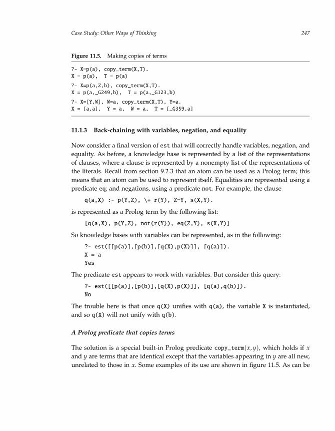
“run” — 2011/9/8 — 18:05 — page 247 — #270�

�

�

�

�

�

�

�


Figure 11.5. Making copies of terms

?- X=p(a), copy_term(X,T).

X = p(a), T = p(a)

?- X=p(a,Z,b), copy_term(X,T).

X = p(a,_G249,b), T = p(a,_G123,b)

?- X=[Y,W], W=a, copy_term(X,T), Y=a.

X = [a,a], Y = a, W = a, T = [_G359,a]

11.1.3 Back-chaining with variables, negation, and equality

Now consider a final version of est that will correctly handle variables, negation, andequality. As before, a knowledge base is represented by a list of the representationsof clauses, where a clause is represented by a nonempty list of the representations ofthe literals. Recall from section 9.2.3 that an atom can be used as a Prolog term; thismeans that an atom can be used to represent itself. Equalities are represented using apredicate eq; and negations, using a predicate not. For example, the clause

q(a,X) :- p(Y,Z), \+ r(Y), Z=Y, s(X,Y).

is represented as a Prolog term by the following list:

[q(a,X), p(Y,Z), not(r(Y)), eq(Z,Y), s(X,Y)]

So knowledge bases with variables can be represented, as in the following:

?- est([[p(a)],[p(b)],[q(X),p(X)]], [q(a)]).

X = a

Yes

The predicate est appears to work with variables. But consider this query:

?- est([[p(a)],[p(b)],[q(X),p(X)]], [q(a),q(b)]).

No

The trouble here is that once q(X) unifies with q(a), the variable X is instantiated,and so q(X) will not unify with q(b).

A Prolog predicate that copies terms

The solution is a special built-in Prolog predicate copy_term(x, y), which holds if xand y are terms that are identical except that the variables appearing in y are all new,unrelated to those in x. Some examples of its use are shown in figure 11.5. As can be

“run” — 2011/9/8 — 18:05 — page 248 — #271�

�

�

�

�

�

�

�

Chapter 11248

Figure 11.6. The final version of back-chaining est.pl

% est(K,Q) holds if query Q can be established from knowledge base K.

% This version performs Prolog back-chaining.

% It handles equality, negation, and variables.

est(_,[]). % No query atoms

est(K,[eq(X,X)|T]) :- est(K,T). % Equality.

est(K,[not(A)|T]) :- \+ est(K,[A]), est(K,T). % Negation.

est(K,[A|T]) :- member_copy([A|B],K), append(B,T,Q), est(K,Q).

% member_copy(X,L): X is an atomic element of L or a copy otherwise.

member_copy(X,L) :- member(X,L), X=[_].

member_copy(X,L) :- member(E,L), \+ E=[_], copy_term(E,X).

seen, copy_term behaves just like Prolog = except in the presence of (uninstantiated)variables.

A final version of the est predicate that handles all the new elements (equality,negation, variables) appears in figure 11.6. Here is how it works:

The first clause is as before;

The second clause handles a query whose first literal is an equality by unifyingthe two arguments and then continuing with the rest of the query.

The third clause handles a query whose first literal is a negation by ensuring thatthe unnegated literal fails and then continuing with the rest of the query.

The fourth clause handles a query whose first literal is an atom. It is as beforeexcept that member_copy is used instead of member.

The member_copy predicate here behaves just like member when the first argumenthappens to be a list with just one element (representing a clause that has no body).Otherwise, member_copy uses copy_term. This has the effect of finding a matchingclause in the knowledge base but leaving its variables uninstantiated for later use.(Assume here that variables only appear in clauses with bodies.)

The following queries illustrate the behavior of the new est predicate:

?- est([[p(a)],[p(b)],[q(X),p(X)]], [q(a),q(b)]).

Yes

?- est([[p(a)],[p(b)],[q(X),p(X)]], [q(Y),not(eq(Y,a))]).

Y = b

Yes

‘‘run’’ --- 2011/9/8 --- 18:05 --- page 249 --- #272�

�

�

�

�

�

�

�


This version of est now handles almost all of Prolog. (It does not yet work withnumbers or built-in operations like write and assert. Also, it does not do the rightthing when the same variable appears in both the query and knowledge base.) Witha bit more work, any Prolog program and any query can be represented as terms andused as arguments to a predicate like est. So this program is a language processor forProlog: a program that can take a symbolic representation of a Prolog program andexecute it. What takes some getting used to, perhaps, is the fact that this processorfor Prolog is written in the Prolog language itself.

11.2 Explanation

Explanation involves finding an atomic sentence such that if it were true, it wouldaccount for a given sentence’s being true. For example, assuming it is known that allpolar bears are white, one would like to be able to explain Thornton’s being white byabducing that he is a polar bear. As it turns out, the final version of the est predicatefrom figure 11.6 makes this possible by using a variable A to stand for the new atomicsentence to be abduced:

?- est([[A],[white(X),polar_bear(X)]],[white(thornton)]).

A = white(thornton) ;

A = polar_bear(thornton) ;

No

The query asks for an atomic sentence A such that if A is added to the knowledgebase, the desired conclusion then follows. There are two such atoms. The first one,white(thornton) is technically correct but only in a trivial way, so one might notwant to consider it as a possible explanation.

11.2.1 Diagnosis

Imagine that a knowledge base has the following facts:

A person will have sore elbows if she has a tennis elbow or sore joints in general.Arthritis will also lead to sore joints. A person will have sore hips if she has sorejoints in general or a hip fracture. Only a tennis player will get tennis elbow.

A representation of this knowledge base is shown in figure 11.7. (The predicatebackground indicates that this list represents background knowledge.) One can thenlook for an explanation for a person Sue’s having a sore elbow:

‘‘run’’ --- 2011/9/8 --- 18:05 --- page 250 --- #273�

�

�

�

�

�

�

�

Chapter 11250

Figure 11.7. A knowledge base about sore joints joints.pl

% What is known about sore joints

background([ [sore_elbow(X), tennis_elbow(X)],

[sore_elbow(X), sore_joints(X)],

[sore_joints(X), arthritis(X)],

[sore_hips(X), sore_joints(X)],

[sore_hips(X), hip_fracture(X)],

[tennis_player(X), tennis_elbow(X)] ]).

% The possible explanations to consider

assumable(tennis_elbow(_)).

assumable(arthritis(_)).

?- background(K), est([[A]|K],[sore_elbow(sue)]).

A = sore_elbow(sue) ;

A = tennis_elbow(sue) ;

A = sore_joints(sue) ;

A = arthritis(sue) ;

No

Thus there are four possible atoms A that could be added as clauses to the backgroundknowledge K to get the desired conclusion. The first atom, sore_elbow, is the trivialexplanation as before. The third atom, sore_joints, may or may not be useful asan explanation. The other two, tennis_elbow and arthritis, are likely the desiredexplanations for sore_elbow.

Often only explanations drawn from some prespecified assumption set or hypothe-sis set are of interest. A typical case of explanation is (medical) diagnosis. In diagnosis,some of the atoms are considered to be possible symptoms, and some of the atomsare considered to be possible diseases. Observations that are among the symptoms aregiven to a diagnostician, and an explanation is sought among the diseases. In gen-eral, what one is willing to assume depends on the problem, and that is what theassumable predicate in figure 11.7 is for:

?- background(K), assumable(A),

est([[A]|K], [sore_elbow(sue)]).

A = tennis_elbow(sue) ;


No

Note that the explanations that are generated depend on what needs to be explained.For example, suppose Sue also has sore hips:

“run” — 2011/9/8 — 18:05 — page 251 — #274�

�

�

�

�

�

�

�


Figure 11.8. A general explanation program explain.pl

% This program uses three predicates defined elsewhere:

% est - the procedure that establishes a query

% background - the background knowledge to be used

% assumable - an atom that can be used in an explanation

% explain(Q,E): Q can be established if E is added to background KB.

explain(Q,E) :- background(K), merge(E,K,K1), est(K1,Q).

% merge(E,K,K1): adding the atoms E as atomic clauses to K produces K1.

merge([],K,K).

merge([A|E],K,[[A]|K1]) :-

merge(E,K,K1), assumable(A), \+ member(A,E).

?- background(K), assumable(A),

est([[A]|K], [sore_elbow(sue),sore_hips(sue)]).


No

In this case, only one explanation does the job; tennis elbow is no longer sufficient. Inother cases, there may be no single atom that gives the desired explanation, and onemay need to look for multiple atoms to assume.

11.2.2 A general explanation program

The general explanation program shown in figure 11.8 attempts to find one or moreatoms to assume. The predicate explain takes two arguments: a query Q that is tobe explained and an explanation E that it will generate as a list of atoms to assume.The merge predicate takes the list of atoms and adds them as atomic clauses to theknowledge base K, checking along the way that they are assumable and that there areno repeats in the list.

The explain predicate can be seen in action by looking at another diagnostic exam-ple, this time involving car trouble (see the knowledge base in figure 11.9). Somequeries for this example appear in figure 11.10.

The first query, without additional assumptions, cannot get an explanation of thecar’s not starting.

The second query shows that a dead battery and being out of gas are both single-atom explanations for the car’s not starting.

The third query shows that being out of gas is the only single-atom explanationfor the car’s not starting when the radio is working.

“run” — 2011/9/8 — 18:05 — page 252 — #275�

�

�

�

�

�

�

�

Chapter 11252

Figure 11.9. A knowledge base about car trouble cars.pl

% The background knowledge

background([

[wipers, not(dead_battery)],

[radio, not(dead_battery), not(broken_speaker)],

[ignition, key_turned, not(dead_battery)],

[car_starts, not(out_of_gas), ignition],

[gauge_shows_gas, not(out_of_gas), not(dead_battery)],

[key_turned]]).

% Things that can go wrong

assumable(dead_battery).

assumable(out_of_gas).

assumable(broken_speaker).

Figure 11.10. Explanations for car trouble

?- explain([not(car_starts)],[]).

No

?- explain([not(car_starts)],[A]).

A = dead_battery ;

A = out_of_gas ;

No

?- explain([not(car_starts),radio],[A]).

A = out_of_gas ;

No

?- explain([not(car_starts),not(radio),wipers],[A]).

No

?- explain([not(car_starts),not(radio),wipers],[A1,A2]).

A1 = broken_speaker, A2 = out_of_gas ;

A1 = out_of_gas, A2 = broken_speaker ;

No

?- explain([not(car_starts),not(radio),wipers],E).

E = [broken_speaker,out_of_gas] ;

E = [out_of_gas,broken_speaker] ;


The fourth query shows that no single-atom suffices to explain all three facts: thecar not starting, the radio not working, the wipers working.

“run” — 2011/9/8 — 18:05 — page 253 — #276�

�

�

�

�

�

�

�


The fifth query shows that there is a double-atom explanation for these threefacts. The explanation is that the car is out of gas and the radio speaker is broken(in either order).

The sixth query looks for an arbitrary explanation under the same conditions. Itfinds the double explanation, but then continues to search indefinitely until allmemory is exhausted.

The last query shows that it is possible to use explain without specifying how manyatomic sentences are desired, but some care is needed.

11.3 Learning

As noted at the start of this chapter, (inductive) learning is a form of thinking that issimilar to explanation except that instead of seeking an atomic sentence to accountfor a query’s being true, it looks for a general rule, that is, a conditional sentence withvariables to explain some observations. If it is known that Thornton and his friendsare polar bears, and they are all observed to be white, it is reasonable to induce thatall polar bears are white. Then on hearing of a new polar bear, one may wish toconclude that she also is white.

The general format for this type of thinking is similar to the explain predicate.Instead of

explain(Q,E) :- background(K), merge(E,K,K1), est(K1,Q).

which generates an explanation E (a list of atoms) that accounts for a given query Q,a predicate induce is defined as follows:

induce(Q,R) :- background(K), rule(R), est([R|K],Q).

The predicate rule generates a conditional sentence R with the property that if it isadded to the background knowledge K, then Q can be established. For example, if thebackground knowledge contains polar_bear(thornton) and polar_bear(shako),the desired behavior is the following:

?- induce([white(thornton),white(shako)],R).

R = [white(_G17), polar_bear(_G17)]

This induced rule (with the variable _G17 in it) says that polar bears are white. Thenext section discusses how to generate rules like this.

“run” — 2011/9/8 — 18:05 — page 254 — #277�

�

�

�

�

�

�

�

Chapter 11254

11.3.1 Inducing general rules

In the simplest case, a rule that explains some observations should have the followingcharacteristics:

The head of the rule should be a predicate in the relevant domain (like polar_bearor white) with variables as arguments.

The body of the rule should be a sequence of literals. Each literal should be apossibly negated predicate in the domain. Moreover, the predicate should bedifferent from the one in the head (to avoid recursion), and the arguments of thepredicate should be among the variables in the head.

So for a rule whose head is r(X,Y,Z), the body can contain the literals not(p(Y)) andq(X,Z,X) but it should not contain r(X,Z,X), which would make the rule recursive,nor q(X,a,W), which uses arguments a and W that do not appear in the head.

The simplest way to satisfy these requirements is to assume that each problemdomain specifies which predicates and which variables can be used. To do this, aspecial predicate called predicate can be used. It plays a role similar to that of theassumable predicate:

predicate(polar_bear(X),polar_bear,[X]).

predicate(white(X),white,[X]).

predicate(bigger_than(X,Y),bigger_than,[X,Y]).

The first argument to predicate is an atom that can be used in the head of a rule;the second argument is the predicate part of the atom as a constant; and the thirdargument is a list of the variables used in the head.

A definition for an induce predicate is presented in figure 11.11. The rule predicateuses the predicate hb (for “head-body”) to generate an atom for the head and a list ofliterals for the body. To deal with the body, in the second clause of hb, each literal L(an atom or its negation) is checked to ensure that its predicate Q is different from thepredicate in the head P, and its arguments U are among the arguments in the head V(using the auxiliary predicate subl). In addition, a negative literal is generated onlyif the rest of the body B is empty or begins with a negative literal.

11.3.2 An example of induction

To show the induce predicate in action, a new knowledge base about animals is pro-vided in figure 11.12. There are a number of individuals that are animals of differenttypes, and a number of predicates to learn about.

“run” — 2011/9/8 — 18:05 — page 255 — #278�

�

�

�

�

�

�

�


Figure 11.11. The induce predicate in Prolog induce.pl

% This program uses three predicates defined elsewhere:

% est - the procedure that establishes a query

% background - the background knowledge to be used

% predicate - an atom that can be used in a rule

induce(Q,R) :- background(K), rule(R), est([R|K],Q).

rule([H|B]) :- hb(H,B,_,_), \+ B=[].

% hb(H,B,P,V): H is an atom with pred P and vars V and

% B is a list of literals with pred not P and vars among the V.

hb(H,[],P,V) :- predicate(H,P,V).

hb(H,[L|B],P,V) :- hb(H,B,P,V), lit(L,Q,U,B), \+ Q=P, subl(U,V).

% lit(L,P,V,B): L is a literal with pred P and vars V, where the

% neg case can only be used if the literals in B are also neg.

lit(A,P,V,_) :- predicate(A,P,V). % the positive case

lit(not(A),P,V,[]) :- predicate(A,P,V). % the 1st neg case

lit(not(A),P,V,[not(_)|_]) :- predicate(A,P,V). % a 2nd case

% subl(L1,L2): the elements of list L1 are all elements of L2.

subl([],_).

subl([X|L1],L2) :- member(X,L2), subl(L1,L2).

Figure 11.12. A knowledge base about animals animals.pl

% An example knowledge base about animals

background([

[animal(X),dog(X)], % Dogs are animals.

[animal(X),cat(X)], % Cats are animals.

[animal(X),duck(X)], % Ducks are animals.

% Some example animals

[dog(fido)], [dog(spot)], [dog(rover)],

[cat(kitty)], [cat(kelly)],

[duck(donald)], [duck(daffy)], [duck(huey)] ]).

% Some predicates to learn about

predicate(animal(X),animal,[X]). predicate(dog(X),dog,[X]).

predicate(cat(X),cat,[X]). predicate(duck(X),duck,[X]).

predicate(barks(X),barks,[X]). predicate(quacks(X),quacks,[X]).

predicate(four_legged(X),four_legged,[X]).

What rule can be learned from observing that Fido barks:

?- induce([barks(fido)], R).

R = [barks(_G404), animal(_G404)] % Every animal barks?

‘‘run’’ --- 2011/9/8 --- 18:05 --- page 256 --- #279�

�

�

�

�

�

�

�

Chapter 11256

The answer is somewhat disappointing: the program induces that every animal barks.While this rule is certainly sufficient to explain Fido’s barking, something more spe-cific is desired. To find a more specific rule, the induce predicate must be given somenegative examples:

?- induce([barks(fido),barks(rover),not(barks(kitty)),

not(barks(donald))], R).

R = [barks(_G425), dog(_G425)] % Every dog barks.

This is a much better rule. Similarly, what rule can be learned from observing thatFido and Kitty are four-legged but Daffy (the duck) is not:

?- induce([four_legged(fido),four_legged(kitty),

not(four_legged(daffy))], R).

R = [four_legged(_G411), not(duck(_G411))]

% Everything that is not a duck has four legs?

This induced rule may or may not be acceptable given what is known. At the veryleast, it should be restricted to animals only, so induce needs to be given informationabout a nonanimal individual, say, a tree:

?- induce([four_legged(fido),four_legged(kitty),

not(four_legged(daffy)),

not(four_legged(tree17))], R).

R = [four_legged(_G428), animal(_G428), not(duck(_G428))]

% Every animal that is not a duck has four legs.

This induced rule has a body with two literals: the individual must be an animal andmust not be a duck.

∗ 11.3.3 Classification: Training and testing

What is the point of inducing new rules? In general, one wants to observe the world,notice the properties of some individuals, induce some general rules about them,and finally, use the general rule to predict the properties of new individuals. So, forexample, after observing that Fido and Rover both bark (but that Kitty and Daffy donot), the induced rule should be able to predict that Spot the dog will also bark.

This type of learning is often called classification: some training examples are given,some of which have a property (like barking) and some of which do not; then newtest examples are classified into those that do and those that do not have the property.

The induce predicate can be used to find out if new individuals have a property. Infact, the new atoms learned from the training examples can be generated:

“run” — 2011/9/8 — 18:05 — page 257 — #280�

�

�

�

�

�

�

�


% Given a query Q as training data (as before), find a new

% atom A that can be established from an induced rule.

learned_atom(Q,A) :-

background(K), induce(Q,R), est([R|K],[A]),

\+ est(K,[A]), \+ member(A,Q).

The learned_atom predicate uses induce to generate a rule as before, then looks foran atom A that is not an element of the training data Q, and that can be establishedgiven that rule, but not without the rule. The result is the following:

?- learned_atom([four_legged(fido),four_legged(kitty),

not(four_legged(daffy)),

not(four_legged(tree17))], A).

A = four_legged(spot) ;

A = four_legged(rover) ;

A = four_legged(kelly)

In this case, enough is learned from the training examples to generate new examples:Spot, Rover, and Kelly are four-legged.

Unfortunately, this simple version of induce looks for ever longer rules to explainthe observations it is given and never actually fails. So if learned_atom is asked toclassify Donald or Huey as four-legged given the same training examples, instead offailing as it should, it would simply run forever.

There are ways of dealing with this issue. The easiest perhaps is to rewrite induceso that it eventually gives up and fails. For example, the length of the desired rulecould be limited. But a better approach is to commit to the first induced rule found bythe program. In other words, if a rule R has been found that accounts for the trainingdata Q, the testing should be done with R, with no backtracking to look for other rules.Prolog provides a built-in predicate called once that does this: if induce(Q,R) in thebody of learned_atom is replaced by once(induce(Q,R)), the program commits tothe first rule found and learned_atom will then fail as it should, for instance, onclassifying the test examples Donald and Huey as four-legged.

In performing such classification, the bulk of the work involves finding a rule thatworks well. When there are a number of predicates to choose from and a numberof variables that are needed, it can be very time-consuming to find a rule that doesthe job properly. This makes it especially important to have training examples thatinclude near-misses, individuals that do not have the desired property but are verysimilar to those that do. With near-misses, it is much easier to locate the negativeliterals that need to be included in the body of the induced rule.

“run” — 2011/9/8 — 18:05 — page 258 — #281�

�

�

�

�

�

�

�

Chapter 11258

11.4 Propositional reasoning

So far, it has been assumed that a knowledge base is made up only of atomic orconditional sentences. This allowed the use of a thinking procedure like back-chainingto draw all the necessary conclusions, and even to do explanation and learning.

But, of course, there are sentences of English that do not fit this pattern. Considerthe following three sentences:

At least one of Alice, Bob, or Carol is guilty.

If Alice is guilty, then so is Bob.

If Alice is not guilty, then neither is Carol.

From these sentences alone, there is no way to tell whether Alice and Carol are guilty.However, it is not hard to see that Bob must be guilty. The reasoning is as follows. IfAlice is guilty, then Bob is also guilty. But if Alice is not guilty, then neither is Carol,and since one of the three must be guilty, it must be Bob. So either way, Bob must beguilty. In other words, the three sentences logically entail that Bob is guilty.

To be able to use knowledge in this sophisticated way, it is necessary to go beyondatomic and conditional sentences to represent what is known, and to go beyond back-chaining to calculate logical entailments. So it is useful to consider a new languagefor representing knowledge, a propositional language, which allows us the expression ofnegations and disjunctions in addition to the previous conjunctions and conditionals.

11.4.1 Conjunctive normal form

Perhaps the simplest representation of a propositional language in Prolog is to usethe conjunctive normal form, or CNF. For present purposes, a CNF formula is a listof disjunctive clauses, or dclauses for short, where a dclause is a list of literals, and aliteral is either an atom or its negation. A dclause is interpreted as the disjunction of itselements, and the entire CNF formula is interpreted as the conjunction of its elements.So the dclause [p,q] is interpreted as saying that p or q is true, and the CNF formula[[p,q],[not(r)]] is interpreted as saying that p or q is true and r is false.

Note that dclauses are interpreted differently from clauses. Previously, a list like[p,q,r,s] represented the conditional “If q and r and s then p.” That same list as adclause represents the disjunction “p or q or r or s.”

And yet there is a definite connection between the two interpretations. Consider aconditional like this:

If q and r and s then p.

“run” — 2011/9/8 — 18:05 — page 259 — #282�

�

�

�

�

�

�

�


That conditional says the same thing as the following disjunction:

not(q) or not(r) or not(s) or p.

To see why, ask what it takes for the conditional to be false. This happens when q, r,and s are true, but p is false. Now what does it take for the disjunction to be false?This happens when all the disjuncts are false, that is, when q, r, and s are true, butp is false. So the conditional and the disjunction are equivalent: they are either bothfalse or both true. This means that the conditional “If q and r and s then p” can alsobe represented by a dclause: [p,not(q),not(r),not(s)]. (The order of the literals ina dclause does not matter.)

In the example with Alice, Bob, and Carol, let the atoms a, b, and c stand forthe guilt of Alice, Bob, and Carol, respectively. Then the three given facts can berepresented as a CNF formula:

[ [a,b,c], [not(a),b], [a,not(c)] ]

This gives the following:

The first dclause says that Alice is guilty or Bob is guilty or Carol is guilty (whichis just another way of saying that at least one of them is guilty).

The second dclause says that Alice is not guilty or Bob is guilty (which is anequivalent way of saying that if Alice is guilty, then so is Bob).

The third dclause says that Alice is guilty or Carol is not guilty (which is anequivalent way of saying that if Alice is not guilty, then neither is Carol).

So every conditional can be represented as a dclause (containing precisely oneunnegated literal), and once it is determined how to calculate logical entailmentsfor CNF formulas in general, that procedure will work for conditionals too.

Although every clause can be rewritten as a dclause, the converse is not true. Forexample, there is no way to represent [not(p)] as a clause. Although there was aform of negation in queries and in the bodies of clauses, there is no way to have asimple negative fact (like Alice is not guilty) in a Prolog knowledge base.

11.4.2 Satisfiability

How does logical entailment work for CNF formulas? So far, a collection of sentencesS1, S2, . . . , Sn logically entails a sentence S if S has to be true when the Si are all true.Another way of saying this is that the sentences {S1, S2, . . . , Sn, not(S)} cannot all betrue. A set of sentences is said to be satisfiable if they can all be true, and unsatisfiableotherwise. So to compute if a collection of sentences Si entails another S, it is sufficient

“run” — 2011/9/8 — 18:05 — page 260 — #283�

�

�

�

�

�

�

�

Chapter 11260

to compute whether a certain set of sentences (formed by adding the negation of S tothe other Si) is satisfiable or not.

But how does one test for satisfiability? For a set of dclauses without variables,there is a very simple account of satisfiability:

A set of dclauses (without variables) is satisfiable if and only if there is a way to picka literal from each dclause without picking both an atom and its negation.

This derives from the fact that a disjunction will be true if one of the disjuncts is true(that is, the literal chosen for that dclause), and a conjunction will be true if all of theconjuncts are true (that is, all the dclauses are true). So, for example, the CNF formula

[ [p], [not(p),not(q)], [not(q)] ]

is satisfiable: pick p from the first dclause, not(q) from the second, and not(q)(already picked) from the third. This means that the dclauses can all be true: ithappens when p is true and q is false.

However, the CNF formula

[ [p], [not(p),not(q)], [q] ]

is unsatisfiable: pick p from the first dclause, which forces the choice of not(q) fromthe second (to avoid having an atom and its negation), and then there is nothing topick from the third. (In other words, the first two dclauses logically entail not(q).)Similarly, the CNF formula

[ [p,q], [not(p),q], [not(q),p], [not(p),not(q)] ]

is unsatisfiable: no matter what is chosen for the first three dclauses, both p and q arepicked, with nothing left to choose from the last one. (In other words, the first threedclauses logically entail both p and q.)

11.4.3 Computing satisfiability

A predicate for testing whether a list of dclauses (without variables) is satisfiable ispresented in figure 11.13. It uses the predicate satpick to go though the dclauses,picking a literal from each one using the predicate pickone. For each dclause, thereare three possibilities (and so three clauses for the pickone predicate):

No new picking is needed if the head of the dclause has already been picked.

The head of the dclause can be picked if its negation has not been picked.

A literal from the tail of the dclause can also be picked.

‘‘run’’ --- 2011/9/8 --- 18:05 --- page 261 --- #284�

�

�

�

�

�

�

�


Figure 11.13. A satisfiability program sat.pl

% The dclauses in DL are satisfied by picking Lits.

sat(DL,Lits) :- satpick(DL,[],Lits).

% satpick(DL,P,Lits): the dclauses in DL can be satisfied by

% picking the literals in Lits, given that those in P are taken.

satpick([],P,P).

satpick([D|DL],P1,Lits) :- pickone(D,P1,P2), satpick(DL,P2,Lits).

pickone([L|_],P,P) :- member(L,P). % L is picked.

pickone([L|_],P,[L|P]) :- \+ member_neg(L,P). % ˜L is not picked.

pickone([_|D],P,P2) :- pickone(D,P,P2). % Use D instead.

member_neg(A,P) :- member(not(A),P).

member_neg(not(A),P) :- member(A,P).

The predicate member_neg is used to check if the negation of a literal has already beenpicked. It does this by either adding or removing a not on the given literal.

It is not hard to confirm that this predicate does the right thing:

?- sat([[p],[not(p),not(q)],[not(q)]],L).

L = [not(q), p]

Yes

?- sat([[p],[not(p),not(q)],[q]],L).

No

?- sat([[p,q],[not(p),q],[not(q),p],[not(p),not(q)]],_).

No

11.4.4 Logical entailment reconsidered

The notion of logical entailment can now be enlarged to deal with knowledge basesthat are lists of dclauses. Continue to assume that there are no variables in thedclauses, and for simplicity, that the queries are as before, a list of atoms or theirnegations, all of which are to be established. It is then easy to do logical entailment:negate the literals in the query and let the sat predicate do the heavy lifting, as shownin figure 11.14.

With this procedure, one can go beyond what was possible with back-chaining. Forexample, the puzzle with Alice, Bob, and Carol can now be solved:

?- estsat([[a,b,c],[not(a),b],[a,not(c)]], [a]).

No

“run” — 2011/9/8 — 18:05 — page 262 — #285�

�

�

�

�

�

�

�

Chapter 11262

Figure 11.14. Entailment using satisfiability estsat.pl

% Dclauses DL entails Q using sat (defined elsewhere).

estsat(DL,Q) :- negs(Q,NQ), \+ sat([NQ|DL],_).

% negs(Q,NQ): NQ is the negation of the literals in Q.

negs([],[]).

negs([not(A)|T],[A|NT]) :- negs(T,NT).

negs([A|T],[not(A)|NT]) :- \+ A=not(_), negs(T,NT).

?- estsat([[a,b,c],[not(a),b],[a,not(c)]], [b]).

Yes

?- estsat([[a,b,c],[not(a),b],[a,not(c)]], [c]).

No

The given facts entail that Bob is guilty, but they do not entail the guilt (or innocence)of Alice or Carol.

The back-chaining examples shown in figure 11.2 can be repeated with theconditionals translated into dclauses:

?- estsat([[a],[b],[u,not(p),not(b)],[p,not(a)]], [b,a]).

Yes

?- estsat([[a],[b],[u,not(p),not(b)],[p,not(a)]], [u]).

Yes

?- estsat([[a],[b],[u,not(p),not(b)],[p,not(a)]], [p,d]).

No

Of course, the way these queries are answered (using the sat predicate) is verydifferent from the back-chaining method used until now.

∗ 11.4.5 First-order reasoning

When a propositional language is enlarged to include variables, it is usually calleda first-order language. Reasoning correctly with a first-order language is much morecomplicated than what has been done so far. For satisfiability, it is no longer sufficientto pick a literal from every dclause; a literal must be picked from every dclause forevery value of the variables in that dclause.

For example, the formula [[not(p(a))],[not(q(b))],[p(X),q(X)]] is consid-ered to be satisfiable, since q(X) can be chosen when X is a, and p(X) otherwise.But the formula [[not(p(a))],[not(q(a))],[p(X),q(X)]] is unsatisfiable, since

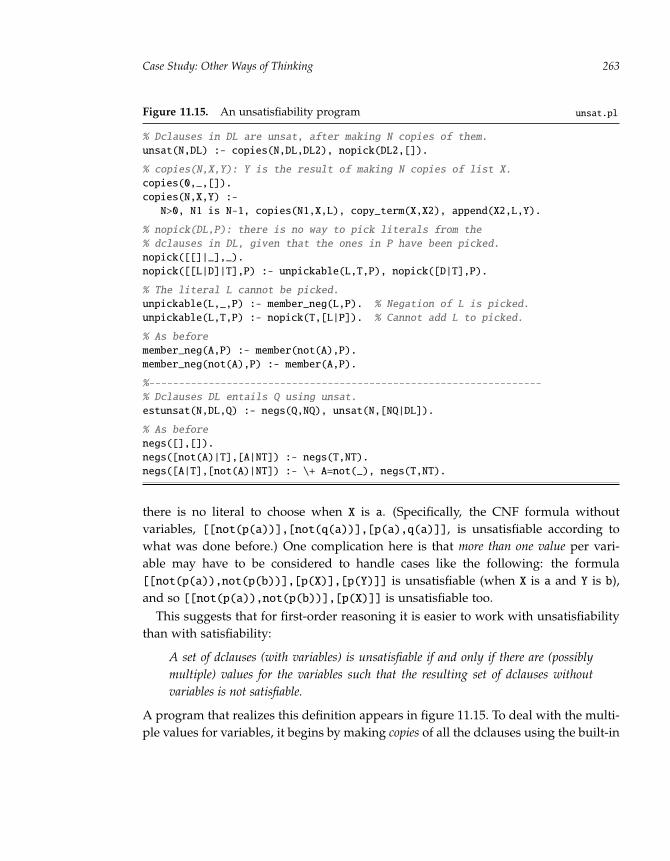
“run” — 2011/9/8 — 18:05 — page 263 — #286�

�

�

�

�

�

�

�


Figure 11.15. An unsatisfiability program unsat.pl

% Dclauses in DL are unsat, after making N copies of them.

unsat(N,DL) :- copies(N,DL,DL2), nopick(DL2,[]).

% copies(N,X,Y): Y is the result of making N copies of list X.

copies(0,_,[]).

copies(N,X,Y) :-

N>0, N1 is N-1, copies(N1,X,L), copy_term(X,X2), append(X2,L,Y).

% nopick(DL,P): there is no way to pick literals from the

% dclauses in DL, given that the ones in P have been picked.

nopick([[]|_],_).

nopick([[L|D]|T],P) :- unpickable(L,T,P), nopick([D|T],P).

% The literal L cannot be picked.

unpickable(L,_,P) :- member_neg(L,P). % Negation of L is picked.

unpickable(L,T,P) :- nopick(T,[L|P]). % Cannot add L to picked.

% As before

member_neg(A,P) :- member(not(A),P).

member_neg(not(A),P) :- member(A,P).

%------------------------------------------------------------------

% Dclauses DL entails Q using unsat.

estunsat(N,DL,Q) :- negs(Q,NQ), unsat(N,[NQ|DL]).

% As before

negs([],[]).

negs([not(A)|T],[A|NT]) :- negs(T,NT).

negs([A|T],[not(A)|NT]) :- \+ A=not(_), negs(T,NT).

there is no literal to choose when X is a. (Specifically, the CNF formula withoutvariables, [[not(p(a))],[not(q(a))],[p(a),q(a)]], is unsatisfiable according towhat was done before.) One complication here is that more than one value per vari-able may have to be considered to handle cases like the following: the formula[[not(p(a)),not(p(b))],[p(X)],[p(Y)]] is unsatisfiable (when X is a and Y is b),and so [[not(p(a)),not(p(b))],[p(X)]] is unsatisfiable too.

This suggests that for first-order reasoning it is easier to work with unsatisfiabilitythan with satisfiability:

A set of dclauses (with variables) is unsatisfiable if and only if there are (possiblymultiple) values for the variables such that the resulting set of dclauses withoutvariables is not satisfiable.

A program that realizes this definition appears in figure 11.15. To deal with the multi-ple values for variables, it begins by making copies of all the dclauses using the built-in

“run” — 2011/9/8 — 18:05 — page 264 — #287�

�

�

�

�

�

�

�

Chapter 11264

copy_term predicate. (It uses a parameter N to decide how many copies to make.) Itthen uses the predicate nopick to confirm that there is no way to pick a literal fromeach dclause in the resulting list. Below the dashed line in the figure, the estunsatpredicate is like the estsat predicate in figure 11.14 except that it uses the success ofunsat rather than the failure of sat to do all the hard work:

?- estunsat(1, [[p(a)],[not(p(X)),q(X)]], [q(a)])

Yes

?- estunsat(1, [[p(a)],[not(p(X)),q(X)]], [q(b)])

No

Note that for some queries it is necessary to use a parameter N > 1:

?- unsat(1, [[not(p(a)),not(p(b))],[p(X)]]). % Wrong.

No

?- unsat(2, [[not(p(a)),not(p(b))],[p(X)]]). % Right.

Yes

Unfortunately, there is no way to know in advance how large a value of N will beneeded to obtain the correct answer.

With a first-order language, more advanced reasoning problems can be handled.Consider the following puzzle (a generalized version was discussed in section 4.4):

There are three blocks, A, B, C, in a stack, with the top one (A) greenand the bottom one (C) not green.

Is there a green block directly on top of a non-green one?

It is clear that the answer must be yes. If B is green, then it is a green one directly ona non-green one (C); if, on the other hand, B is not green, then the top block (A) is agreen one directly on a non-green one (B). Either way, the conclusion follows.

What makes this puzzle challenging is that we know there has to be a green blockdirectly on top of a non-green one, and yet we cannot say which one it is. With back-chaining, whenever it was known that something had a property, enough informationwas always given to figure out what that something was. First-order reasoning usingestunsat is more general and does not have this limitation:

?- estunsat(2,

[ [on(a,b)], [on(b,c)], % The facts

[green(a)], [not(green(c))] ], % More facts

[ on(X,Y), green(X), not(green(Y))] ). % The query

Yes

“run” — 2011/9/8 — 18:05 — page 265 — #288�

�

�

�

�

�

�

�


Observe that the only thing that prevents representing all the given facts as a set ofclauses in Prolog (and using normal back-chaining) is the fact about the bottom blocknot being green. But to handle this negative fact properly and to fully use what isknown requires thinking in this new advanced way.

Want to read more?

This chapter explored ways of thinking that went beyond simple back-chaining.Remarkably enough, these new ways of thinking were all formulated in terms ofback-chaining.

The idea of using a programming language to write a language processor for thatvery language (a meta-interpreter) is a practice developed to a fine art in the LISPcommunity [53], which uses this idea in a number of ways, including adding newprimitive constructs to the language. In this chapter it was used to explore variantsof the Prolog processor and to handle abduction and induction by making temporaryadditions to the underlying knowledge base.

The section on explanation took a first glance at an area of research called abductivelogic programming (for example, see [54]). The section on learning introduced the areaof inductive logic programming (for example, see [56]). These two continue to be activeareas of research, although techniques more closely allied with probability theoryhave gradually come to dominate the study of both diagnosis and learning.

The section on propositional reasoning is perhaps the most open-ended part of thebook. Its generalization of clauses to dclauses allowed representing a much widerrange of knowledge, in particular, incomplete knowledge, when certain facts must beconsidered even though their truth is unknown (like the guilt of Alice). When vari-ables and a few other features are included, the resulting first-order logic is the typicalstarting point for logical reasoning within AI, for example in [4].

Computing satisfiability (for CNF formulas without variables) has become an activearea of AI research. It turns out that many of the problems considered in this book(including constraint satisfaction and planning) can be reformulated directly in termsof satisfiability. This is significant because there have been great advances in recentprograms that compute satisfiability [55].

Computing unsatisfiability (for CNF formulas with variables) is also an active areaof research called automated theorem-proving [57]. The emphasis is on taking (small)parts of mathematics, formalizing them as a set of axioms in a first-order logic, and

“run” — 2011/9/8 — 18:05 — page 266 — #289�

�

�

�

�

�

�

�

Chapter 11266

then asking if they entail some mathematical conjecture of interest. In 1996 an auto-mated theorem-proving program written by William McCune and colleagues was ableto prove Robbins’ Conjecture, a statement in algebra whose status had remained openfor sixty years.

All the reasoning in this book comes out as a special case of first-order reasoning.This means (in theory) leaving Prolog behind and continuing the work using a first-order logic instead. Prolog is a conceptual ladder of great value, but now one can kickthe ladder away and explore along different paths.

“run” — 2011/9/8 — 18:05 — page 267 — #290�

�

�

�

�

�

�

�

12 Can Computers Really Think?

This is a book about thinking. Looking at a wide range of behaviors that appear todepend on thinking, it showed how they could be realized in computer programs:solving recreational puzzles, interpreting visual scenes, understanding Englishexpressions, planning courses of action, playing games, and some forms of explana-tion and learning. Only simple versions of these activities were considered, of course,but in each case, thinking—bringing knowledge to bear on the activity—could beunderstood as a form of computation.

What can be learned from this? Perhaps the following:

It is possible to get computers to do fairly impressive things even with smallprograms. (All the programs in this book are well under one hundred lines long.)What is needed is a programming language that allows stating what needs to beknown to perform the task.

It is indeed possible to interpret at least some forms of thinking as com-putation. What needs to be known can be represented as a collection of(atomic and conditional) sentences, from which conclusions can be drawn usingback-chaining.

The real issue is not so much whether intelligent behavior can be produced atall but how well. Almost all the tasks considered (puzzles, language, planning,games, and so on) worked in simple versions, but as the problems got biggerand more complex, the basic methods did not scale well.

Not surprisingly, the bulk of the research in artificial intelligence (AI) is concernedwith how to achieve intelligent behavior in complex situations where simple tech-niques do not work (like playing chess and Go, rather than tic-tac-toe, for instance).The book showed some of the ways of dealing with this complexity:

how to do better than basic generate-and-test;

how to represent action and change for large worlds;

how to play games without searching the entire game tree; . . .

“run” — 2011/9/8 — 18:05 — page 268 — #291�

�

�

�

�

�

�

�

Chapter 12268

Of course, there is a lot of thinking that the book did not talk about at all. Whatabout the thinking that goes into designing a bridge or composing a piece of music?What about following the dialogue in a play? What about the sort of thinking thatoccurs when recalling a childhood event or daydreaming? What about meditation?What about the role of emotion? An account of thinking that is true to the very widerange of mental experiences people have would go well beyond what was consideredhere.

But nonetheless, even within a limited context, and despite all the restrictions, thisbook still raises a philosophical question. If it is true that thinking (or some forms ofit) can be understood as computation, does it then not follow that given the rightprogram, a computer is able to think?

For many people, this is a very troubling idea. Thinking and the intelligent behaviorit gives rise to feel very special to us. At its most elevated, we might say, thinkingdefines what it means to be human. The idea that a gadget like an electronic computermight also be able to think is unsettling.

Looking back at what was accomplished in previous chapters, was it really possi-ble to program a computer to think about the grandfather relation, the objects in ascene, the words in a sentence, the ways to achieve a goal? Or was the computer justprogrammed to behave as if it were thinking? Is there a difference?

This final chapter briefly explores these philosophical questions.

12.1 What computers can do

Can a computer really think? Before answering, consider a question that is evenmore basic: Can a computer really add two numbers? Many of us, would say yes: asuitably programmed computer can take two numbers as input and return their sumas output. Nobody disputes this. If this is not adding two numbers, then what is?

But nothing is taken for granted in philosophy. In fact, some might be tempted byan account like the following:

Computers cannot do addition, really. All they can do is mechanically shufflearound uninterpreted symbols. It is we, the human beings, who interpret thisshuffling. In some cases, we might interpret it as addition, say. But this is up tous, and someone else might interpret the shuffling completely differently, likesolving a puzzle or playing some sort of mysterious game. At any rate, for thecomputer itself, no arithmetic is involved.

“run” — 2011/9/8 — 18:05 — page 269 — #292�

�

�

�

�

�

�

�

Can Computers Really Think? 269

If this is the way one chooses to talk about computers, the discussion stops here.There is really no point in talking about whether they can think if one is not evenwilling to concede that they can add.

This is not a particularly helpful way of talking, however. Imagine we are studyingthe bewildering game of Go and wondering whether a computer has ever won againsta Go champion. Suppose we get an answer like this:

No computer has ever beat a Go champion because a computer cannot even playthe game of Go. All it can do is move around meaningless symbols.

This way of talking is not helpful because it does not make the simple distinctionswe are looking for. We want to be able to say that yes, a computer did win againsta chess champion (once), but no, a computer has not yet beat a Go champion. Butin talking this way, we are allowing that computers can indeed do things like addnumbers, solve Sudoku puzzles, and play world-class chess. (You can’t win at chess ifyou can’t even play chess!)

In essence, we are saying that the computer’s external behavior (as given by theinputs and outputs) is enough for us to judge. We do not need to know about thehidden internal state of the computer or whether there are other interpretations ofthe inputs and outputs. Fortunately, this is the way most people choose to talk aboutcomputers.

(As a side note, there is something right about shifting the question about whatcomputers can do to the question about what people can do. When we ask, “Can acomputer play decent Go?” what we are really asking is, “Is there a suitable computerprogram?” that is, a program that when run on a general-purpose computer producesthe external behavior we want in a reasonable amount of time. And to go further, itis not just a program’s existence that matters; we might know that there must be sucha program without anyone’s knowing how to write it. Our question is really, “Hasanyone been able to write a suitable program?” So the question is really about people!When we say that the Deep Blue computer beat a chess champion, and we applaudthat achievement, it is really the team from IBM that produced Deep Blue that weare applauding. Of course, some day, we may be more willing to give credit to themachine itself; but that’s for another day.)

Now let us return to the original question: Can a computer really think? Can itunderstand English? Can it be intelligent? Here we do not seem to be talking about thecomputer’s external behavior but about its internal workings, not just what a computercan do, but what it can be.

“run” — 2011/9/8 — 18:05 — page 270 — #293�

�

�

�

�

�

�

�

Chapter 12270

12.2 The Turing Test

In the 1950s, Alan Turing wrote a now famous philosophical paper [66] arguingthat terms like thinking, understanding, being intelligent are just too vague to be worthspending time arguing about. One can imagine, for instance, two critics going backand forth never being able to agree on whether real thinking or real understanding wastaking place. Instead, Turing proposed, we should return to behavior in the followingthought experiment.

Imagine that you have a long-distance typed conversation over a terminal with twoother parties. One of them is a person, and the other is a computer program. Theconversation is natural, free-flowing, and about any topic you desire. Neither partyis stonewalling or trying to steer the conversation in any way. Now imagine that nomatter how long the conversation goes on, you cannot figure out which of the twoparties you are talking to is the person and which is the computer. We would say thatthe computer has passed the Turing Test.

Roughly speaking, Turing’s position amounts to this. If we insist on using terms likethinking or understanding, we should be willing to accept that anything that passes thistest is thinking or understanding as much as a person is. We are of course perfectlyfree to say that something is not thinking if it does not look like we do, or does nothave a brain, or is not connected to a physical world the way we are, and so on. We arefree to say this, but in the end, this is just a form of chauvinism, not so different fromsexism or racism. We should concede that anything that can behave as intelligently aswe do is as intelligent as we are.

(We might be wrong, of course. But we could be wrong about the person we havebeen talking to as well. This “person” might actually be some sort of zombie fromouter space, somehow able to fake a conversation without any understanding, orwithout any internal mental life. These are possibilities, but they are just too far-fetched to be worth spending any time on.)

So for Turing, external behavior is what counts. To paraphrase the Forrest Gumpmovie character, Intelligent is as intelligent does!

Turing’s argument is compelling, and most computer scientists today probablyaccept it. This explains why scientists in artificial intelligence see their job as dealingwith intelligent behavior of various sorts and spend almost no time discussing whetherreal understanding (say) is taking place. This is what was done in this book: it studiedwhat was needed to get the desired external behavior in a variety of domains.

“run” — 2011/9/8 — 18:05 — page 271 — #294�

�

�

�

�

�

�

�


12.3 The Chinese Room

But philosophers are an obstinate lot. They are not going to back down on the issueof whether real understanding is taking place just because someone like Turing saysthey should. Perhaps the most successful attack on Turing’s position came from thephilosopher John Searle in the 1980s. He devised a different thought experimentto argue that there was much more to understanding (or thinking, or being intelli-gent) than merely getting the external behavior right. Here is (a slight variant of) hisargument.

Imagine that there is already a computer program that is somehow able to pass theTuring Test, but in Chinese, not in English. Let us call the computer program thatdoes this chinese.pl, assuming it is written in Prolog. So Chinese characters can bepresented to this program (encoded in some way), and it will produce responses (alsoencoded in some way) that cannot be distinguished even over a long period of timefrom those of a person who really understands Chinese.

Now imagine that Searle does not know Chinese, but knows Prolog very well. Heis put in a room with a book that contains the text of the chinese.pl program. Whensomeone outside the room slips him pieces of paper with Chinese written on them, hedoes not understand them, but he can follow what chinese.pl would do given theseas input. He traces the behavior of the program, writes on a piece of paper the outputthat the program would produce, and hands that back, again without understandingwhat any of it means.

So there is a person, Searle, who is receiving Chinese messages and producing Chi-nese responses no different from those of a native Chinese speaker (since chinese.plis assumed to pass the Turing Test). His external behavior, in other words, is per-fect. And yet Searle does not know Chinese. Searle’s conclusion: getting the externalbehavior right is not enough, and so Turing is wrong.

A counterargument is that Searle is not producing this behavior, but Searle togetherwith the book. Although Searle does not understand Chinese, the system consistingof Searle and the book does. So Turing is not wrong. Searle’s reply to this objectionis beautiful in its simplicity: Imagine that he memorizes the book and then destroys it.Then there is no longer a system to talk about; there is just Searle. So Turing is wrong.

Is this the last word on the topic? Remember, nothing is obvious in philosophy.Consider this: How can we be so sure that Searle does not come to learn Chinese aftermemorizing the book? If he did, then the argument would collapse. The answer isthat we do not know what happens after he learns the book simply because we do

“run” — 2011/9/8 — 18:05 — page 272 — #295�

�

�

�

�

�

�

�

Chapter 12272

not have a clear picture of what this imagined chinese.pl program would have tobe like (assuming it can exist at all). But we can get some clarification by turning to asimpler case, addition again.

12.4 The Summation Room

Imagine a room with a person in it who does not know how to add numbers. Mes-sages are passed to the person on a sheet of paper containing a list of twenty numbers,each of which has ten digits. The book inside the room that he is able to use is a verylarge one: it has ten billion chapters, and each chapter has ten billion sections, andeach section has ten billion subsections, and so on, up to depth twenty. The prefaceof the book has the following instructions:

Take the first number in the list of twenty and go to that chapter; then take thesecond number in the list and go to that section; then take the third number andgo to that subsection; and so on until all twenty numbers have been used up. Atthe end of this process, there will be a number written in the book with at mosttwelve digits. Write that number on a slip of paper and hand it back outside theroom.

Unbeknownst to the person in the room, the book is constructed in such a way thatthe twelve-digit entries in the book are in fact the sums of the twenty numbers thatled to the entry.

Now the person in the room, following the procedure in the book, is clearly notadding. He is producing the correct sums, of course, but only by looking them up.This is no different from phoning a friend and getting the answers from her. And whatif the person were to somehow memorize the contents of the book and follow theinstructions mentally? To an observer, the person would be examining the numbers,reflecting for a while, and then writing down their sum. From the outside, it wouldlook just like the numbers were being added, but they are not.

This, in a nutshell, is Searle’s argument but now applied to addition. The person inthe room is producing the right external behavior but does not know how to add.

So does this mean that Searle is right after all? Not quite. There is a serious flawin the argument with the Summation Room: the book needed for the thought experimentcannot possibly exist. It would have to contain 10200 entries, but the entire physicaluniverse only has about 10100 atoms. So a thought experiment that relies on this bookis vacuous. It might work if we only had to add two ten-digit numbers, say, but fortwenty or more, this is too much for our universe.

“run” — 2011/9/8 — 18:05 — page 273 — #296�

�

�

�

�

�

�

�


However, there is a smaller book that would do the job for the twenty numbers.Consider a book that contained the procedures PROC0, PROC1, PROC2, and PROC3from chapter 1. This book can certainly exist. In fact, it would be more like a smallpamphlet, and the instructions there would allow the person in the room to producethe correct sums.

However, notice what happens this time when the person in the room memorizesthe instructions in the pamphlet: he learns how to add. In fact, most of us learned howto add by being given instructions like those in the pamphlet. So the man in the roomdoes get the right answers, but now he also knows how to add.

This is enough to cast some doubt on Searle’s Chinese Room argument. Perhapsadding two ten-digit numbers is simple enough that a big table of answers wouldallow someone to fake it. But adding twenty ten-digit numbers appears to be complexenough that a book that does the job would also end up teaching the person in theroom how to add. Beyond some level, if you need to get the sums out, you will not beable to fake it; you will need to do the addition. So why should we think that Chinese(however that book turns out) is going to be any easier to fake? It might be moresensible to conclude that once a behavior is complex enough (on the order of addingtwenty ten-digit numbers, say), insisting that the behavior be right will be enough torule out various forms of tricks or fakery.

12.5 A final word

So does this settle the question as to whether a computer can think? No, not at all.At best, it casts doubt on Searle’s refutation of Turing’s position, which was that weshould not even ask this question in the first place. And new and improved argumentson this topic may yet appear.

But no matter what one’s position on the philosophical issues, we are still left withwhat might be called the AI question: If it is indeed true that tricks and fakery are notsufficient to generate intelligent behavior such as passing some form of the TuringTest, then what is? In the end, it is this question that is perhaps the most profound oneto emerge out of the entire discussion, and one that will not be resolved by merelyarguing one way or another.

And where to look for a possible answer is what this book has been about.

“run” — 2011/9/8 — 18:05 — page 274 — #297�

�

�

�

�

�

�

�

Chapter 12274

Want to read more?

The issues presented in this chapter are part of what is usually called the philosophyof mind, an area of research well represented in most departments of philosophy andin various articles in [59].

This area began more or less with the writings of Rene Descartes (1596–1650),who wondered how an intangible mind could interact with a physical body (theso-called mind-body problem). Although there was always a fascination with a vari-ety of automata, attention shifted decisively to computers as soon as they becamewidely known. Turing’s paper introducing the Turing Test [66] was perhaps a water-shed point in this evolution, although he did what he could to stand outside the areaand quell further discussion. Searle’s paper on the Chinese Room [64] was anothermilestone that resulted in a flurry of replies and commentary, including my ownSummation Room argument [61]. Although the ideas in Searle’s paper may seemfrustratingly naive to many computer scientists, they have withstood the test of time.

There are many other aspects of the philosophy of mind that have not even beentouched on here. Among them are the following: Jerry Fodor argues for a “mentalese”that has many of the properties of natural languages [60]; Daniel Dennett and manyothers study properties of consciousness [58]; and there are many who argue thatthe human mind cannot be computational, based on considerations such as Godel’sIncompleteness Theorem [62] and even quantum mechanics [63].

But perhaps the most thought-provoking philosophy related to thinking and com-putation is the work of Brian Cantwell Smith, for example [65]. His writing canbe hard to read and is not about the philosophy of mind at all, but more on theother side of the street, the philosophy of computation. Smith argues (convincingly)that computation must be understood as more than shuffling around uninterpretedsymbols. His view is that in some cases the interpretation of the symbols matters tothe computation, although in many cases that interpretation is outside the “causalreach” of the person or computer using the symbols. His attempt to formulate theapproach to knowledge taken in this book, but taking into account this richer notionof computation, is what he calls the knowledge representation hypothesis (see [1], p. 6).

“run” — 2011/9/8 — 18:05 — page 275 — #298�

�

�

�

�

�

�

�

Appendix ASome Computer Basics

To make good use of this book, you need to be able to perform some simple operationson a computer. (You do not need to know how to program a computer.) Mainly theseinvolve creating, deleting, editing, saving, and printing ordinary text files, as well asviewing and printing PDF files.

If you are using this book as part of a course, find the website site for this book,which contains a number of useful files.

A.1 Working with computer files

Here is a checklist of operations you should be able to do comfortably as you start touse the book:

1. View these instructions on a computer screen. Go to the book website which hasa file called basics.pdf that contains this appendix in PDF format.

2. Print these instructions on a computer printer.

3. Save these instructions in a file on your computer called basics.pdf. You shouldalso be able to come back to your computer later, find your copy of the file onyour computer, and view it on your screen.

4. Delete the file basics.pdf from your computer, and go back to reading the onlineversion of the file at the book website for the next step.

5. Go to the book website and find the file basics.pl. Click on the file, and down-load it to your computer. This is a text file that contains a simple program in thelanguage Prolog. Your computer won’t be able to do much with the file yet.

6. Make a copy of the file basics.pl and call it origbasics.pl. This one is forsafekeeping.

7. View the contents of the file basics.pl in a text editor on your computer. Youcan use a basic editor like Notepad (Windows) or TextEdit (Mac) or nedit (Linux),or a fancier one like Microsoft Word or vi or emacs. Windows and Mac users: Youwill not be able to simply double-click the file; you will need to start the editorfirst and then open the file from there.

‘‘run’’ --- 2011/9/8 --- 18:05 --- page 276 --- #299�

�

�

�

�

�

�

�

Appendix A276

8. Change the line in the file that says

myname(’Sydney J. Hurtubise’).

so that your name appears between the single quotes.

9. Save the changed file as mybasics.pl on your computer. This needs to be savedas an ordinary text file, meaning no bold or italics, or anything with fonts or specialformatting. These files are sometimes called text-only or plain-text or ASCII orno-formatting.

10. Exit the editor leaving the file basics.pl unsaved and in its original state. Itshould be identical to origbasics.pl.

11. Print the file mybasics.pl on your printer and confirm that your name appearsbetween the single quotes.

That’s it. If you can successfully perform all these tasks, you are as computer-literateas you need to be.

A.2 Files available online

Here are all the files that should be available online at the book website fordownloading. First, there are the following special files:

basics.pdf: This appendix as a PDF filebasics.pl: A sample text fileapplescript.txt: A file for Mac OS X users (figure B.1, page 281)wordUtils.pl: A Prolog utility file used in chapter 8 (page 170)

Finally, there are all the example Prolog programs that are presented in the text:

family.pl: The family example in Prolog (figure 3.1, page 42)likes.pl: The likes example (figure 3.11, page 56)blocks.pl: A blocks-world program (figure 4.2, page 67)left.pl: A better procedure for the left predicate (figure 4.6, page 80)map.pl: Coloring the map of figure 5.1 (figure 5.2, page 88)sudoku.pl: A Sudoku solver (figure 5.5, page 93)factorial.pl: A program for n! (figure 5.7, page 99)sendmore1.pl: SEND+MORE=MONEY v1 (figure 5.8, page 100)sendmore2.pl: SEND+MORE=MONEY v2 (figure 5.9, page 102)

‘‘run’’ --- 2011/9/8 --- 18:05 --- page 277 --- #300�

�

�

�

�

�

�

�

Some Computer Basics 277

cap.pl: Testing if one queen can capture another (figure 5.12, page 105)queens.pl: A solution to the eight-queens problem (figure 5.13, page 105)logic1.pl: A solution to the first logic problem (figure 5.15, page 108)logic2.pl: A solution to the second logic problem (figure 5.16, page 109)zebra.pl: A solution to the zebra problem (figure 5.17, page 111)schedule-top.pl: A classroom scheduler (figure 5.19, page 114)schedule-aux.pl: Previously scheduled periods (figure 5.20, page 114)regions.pl: The types of regions and their properties (figure 6.4, page 123)sketch.pl: The sketch map interpretation (figure 6.6, page 124)polyrules.pl: Permissible vertices in Prolog (figure 6.10, page 127)polyinterp.pl: Interpreting the edges in figure 6.7 (figure 6.11, page 128)cuboid.pl: Finding a cuboid in an image (figure 6.15, page 131)occlusion.pl: Finding vertices with occlusion (figure 6.17, page 134)blocks2.pl: The blocks-world program redone (figure 7.3, page 148)nldb.pl: A world of people, parks, trees, hats (figure 8.4, page 160)lexicon.pl: A lexicon in Prolog (figure 8.5, page 161)np.pl: A parser of noun phrases in Prolog (figure 8.6, page 163)yesno.pl: A parser for yes/no questions (figure 8.14, page 171)declarative.pl: A parser for declaratives (figure 8.15, page 174)plan.pl: A general planner in Prolog (figure 9.3, page 184)coins.pl: The three-coins problem in Prolog (figure 9.4, page 184)monkey.pl: The monkey and bananas problem in Prolog (figure 9.6, page 187)bplan.pl: A general but bounded planner (figure 9.8, page 189)puzzle2x3.pl: A 2 x 3 version of the 15-puzzle (figure 9.11, page 191)splan.pl: A staged planner in Prolog (figure 9.13, page 195)raceto21.pl: A Prolog program for Race to 21 (figure 10.2, page 212)gameplayer.pl: A general game player (figure 10.5, page 216)tictactoe.pl: A Prolog program for tic-tac-toe (figure 10.6, page 219)playuser.pl: Playing an entire game (figure 10.7, page 221)boxes.pl: A Prolog program for Boxes (figure 10.13, page 225)minimax.pl: A minimax procedure in Prolog (figure 10.17, page 230)estfc.pl: A forward-chaining procedure (figure 11.4, page 246)est.pl: The final version of back-chaining (figure 11.6, page 248)joints.pl: A knowledge base about sore joints (figure 11.7, page 250)explain.pl: A general explanation program (figure 11.8, page 251)cars.pl: A knowledge base about car trouble (figure 11.9, page 252)

“run” — 2011/9/8 — 18:05 — page 278 — #301�

�

�

�

�

�

�

�

Appendix A278

induce.pl: The induce predicate in Prolog (figure 11.11, page 255)animals.pl: A knowledge base about animals (figure 11.12, page 255)sat.pl: A satisfiability program (figure 11.13, page 261)estsat.pl: Entailment using satisfiability (figure 11.14, page 262)unsat.pl: An unsatisfiability program (figure 11.15, page 263)

“run” — 2011/9/8 — 18:05 — page 279 — #302�

�

�

�

�

�

�

�

Appendix BGetting Started with SWI-Prolog

To be able to follow the many Prolog examples in the book and to run your ownprograms, you will need to have access to a Prolog system installed on the computeryou are using. To simplify matters, the book only discusses the SWI-Prolog system. Iffor some reason, you are forced to deal with another dialect of Prolog, see appendix Dfor some of the differences you may run into.

Ideally, a computer expert will install SWI-Prolog for you on your computer andtell you what to do with your Prolog files. From that point on, everything else youneed to know is covered in this book starting in chapter 3.

In case there is no computer expert around, you will need to do the installationyourself. Take it slowly, make sure everything works as you go, and get as muchhelp as you can. Section B.1 deals with the installation of SWI-Prolog, and section B.2covers how to load and run your own Prolog programs.

Warning. The instructions in this appendix may go out of date. Computers change,operating systems (Windows, Mac, Linux) change, and Prolog systems change. Iftoo much has changed, these instructions may no longer work and you will needhelp from an expert.

B.1 Installing SWI-Prolog

This section concerns installing the free SWI-Prolog software on a computer that youcontrol. If you are using a shared computer, as in a lab at a university, you will notbe able to install any software yourself. If SWI-Prolog is already installed, you are inluck; find out how to start it, and then go on to the next section. If SWI-Prolog is notinstalled, you will need to ask around to see what your options are; another dialectof Prolog may be installed, or you may be out of luck.

With Windows

To install SWI-Prolog under Windows, begin by downloading an installation packagefrom http://www.swi-prolog.org/download/stable/. The latest version of SWI-Prolog should run under the latest version of Windows. (Note: You can always safelyuse a 32-bit version.) Then follow the installation instructions.

“run” — 2011/9/8 — 18:05 — page 280 — #303�

�

�

�

�

�

�

�

Appendix B280

With Mac OS X

To install SWI-Prolog under Mac OS X, begin by downloading an installation packagefrom http://www.swi-prolog.org/download/stable/. You will need to know whichversion of Mac OS X you are using (which you can see by selecting “About This Mac”under the Apple menu): 10.4 (Tiger), 10.5 (Leopard), 10.6 (Snow Leopard), or later.Then follow the installation instructions. (Note to experts: If MacPorts is installed,SWI-Prolog can be installed from there. Either way, the SWI-Prolog binary will beinstalled as /opt/local/bin/swipl.)

With Linux

The SWI-Prolog binary comes preinstalled on some Linux systems. If so, you arein luck as there is no easy way to do the installation. There is an RPM file athttp://www.swi-prolog.org/download/stable/, but it may not be right for yoursystem. There are sources online, but if you have never installed a Linux programfrom sources before, you will definitely need help.

B.2 How to load SWI-Prolog programs

Once you have installed SWI-Prolog, you are ready to use it with some Prolog pro-grams that you have written yourself or downloaded and saved on your hard drive.For example, assume you have saved the file family.pl (figure 3.1). This program isavailable on the book website (see appendix A) and will be used here as an example.

With Windows

Once SWI-Prolog has been installed on a Windows system, any file whose name endswith .pl (such as family.pl) will be known to the system as a Prolog program.You can double-click the file, and this will start SWI-Prolog and automatically loadthat Prolog program. It is therefore unnecessary to use the square bracket notationto manually load the program, as done in figure 3.2. (However, additional Prologprograms in the same folder as the file can be loaded with the square bracket notationas required.) When you are finished with Prolog, close the Prolog window to exit.

“run” — 2011/9/8 — 18:05 — page 281 — #304�

�

�

�

�

�

�

�

Getting Started with SWI-Prolog 281

Figure B.1. An AppleScript for SWI-Prolog

on run

set prolog to "/opt/local/bin/swipl"

set myprompt to "Where do you keep your Prolog programs?"

set dir to POSIX path of (choose folder with prompt myprompt)

tell application "Terminal"

activate

do script "cd \"" & dir & "\"; " & prolog in window 1

end tell

end run

With Mac OS X

Unfortunately, running SWI-Prolog with a Mac is not as easy as it could be. It is bestto begin by preparing an AppleScript. Start the AppleScript Editor (often located inthe Utilities folder within the Applications folder). In the untitled window thatit presents, insert the text from the figure B.1 exactly as is. (The text can be cut andpasted from the file applescript.txt that is on the book website. See appendix A.)Then do a “Save As” to save the script: choose the file format “application,” use aname like “Start-SWI,” and save it to your desktop.

Once “Start-SWI” has been saved, Prolog can be used as follows:

1. To start Prolog, double-click the “Start-SWI” icon on your desktop.

2. It will ask you where you keep your Prolog programs. Navigate to a folder, suchas the folder that contains family.pl, and hit the “Choose” button.

3. From within Prolog, you can now load any Prolog program in that folder byusing the square bracket notation (as done in figure 3.2).

4. When you are done with Prolog, quit the Terminal application.

With Linux

After installing SWI-Prolog, there should be a binary called swipl. To use it, firstconnect using cd to the directory that contains your Prolog programs like family.pl,and then start Prolog. From there, interact with Prolog, as shown in figure 3.2.

“run” — 2011/9/8 — 18:05 — page 282 — #305�

�

�

�

�

�

�

�

“run” — 2011/9/8 — 18:05 — page 283 — #306�

�

�

�

�

�

�

�

Appendix CGetting Your Prolog Programs to Work

I assume that SWI-Prolog has been installed, and that the family.pl program worksfor you just like in figure 3.2. (Otherwise, see appendix B.) This appendix considershow to use some of the features of SWI-Prolog to get new Prolog programs that youwrite to work as intended. (There are, of course, many ways of doing this, but whatfollows are my recommendations.)

When you are using SWI-Prolog on your computer, keep two windows open andwork as follows:

1. Start your text editor (see appendix A), and either type in or open the current ver-sion of your own Prolog program. Save the file (with a name like something.pl),but keep this window open.

2. Start Prolog and load the current version of your program (as described forfamily.pl in appendix B). This will be your second window.

3. Try some Prolog queries in the Prolog window.

4. If the queries all work as expected, then you are done. You may want to save somequeries and their results for the record. Then quit Prolog and the text editor.

5. If some queries do not work as expected, find out what went wrong, make somechanges in the text editor window, save the file, and then reload the programinto Prolog. Then go back to step 3.

Let us go through these steps to see what can go wrong.

C.1 Getting program files to load

One problem you may have is that you try to load a program file (using the squarebrackets), but the file is not found:

?- [block].

ERROR: source_sink ‘block’ does not exist

‘‘run’’ --- 2011/9/8 --- 18:05 --- page 284 --- #307�

�

�

�

�

�

�

�

Appendix C284

The special predicate ls can be used to see what files are in the current folder and areavailable to be loaded:

?- ls.

blocks.pl grid.pdf myfamily.pl

daisy.jpg monkey.pl planner.pl

Yes

?- [blocks].

% blocks compiled 0.00 sec, 2,088 bytesYes

Note that ls lists all the files in the current folder. Only the files whose names endwith .pl, such as blocks.pl, can be loaded. It is sometimes necessary to load two ormore files, which can be done as follows:

?- [planner,monkey].

% planner compiled 0.00 sec, 1,432 bytes

% monkey compiled 0.00 sec, 2,012 bytes

Yes

The next thing to worry about is that Prolog finds your file but cannot load it withoutan error:

?- [myfamily].

ERROR: myfamily.pl:4:0: Syntax error: Operator expected

% myfamily compiled 0.00 sec, 1,400 bytes

Yes

This error means that myfamily.pl is not yet a legal Prolog program. Typically,punctuation of some sort is wrong. Here is a listing of the myfamily.pl file:

child(henry,hanna).

male(henry)

female(hanna).

mother(X,Y) :- child(Y,X), female(Y).

As can be seen, there is a missing period at the end of the second clause. Prologreports where it runs into trouble. The myfamily.pl:4:0 on the error line means thatit was at line 4 column 0. (The actual error is typically somewhere nearby. It is a goodidea to use a text editor like Notepad or TextEdit that allows you to easily get to aline in a file by its line number.)

Here is what you need to do: Go to the text editor window, find the grammaticalerror, change the file, and save the new version of the file. Then go back to the Prologwindow, and use the special predicate make to reload the file into Prolog:

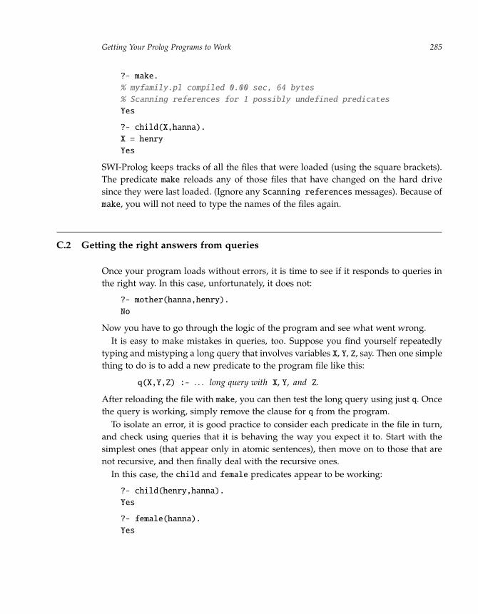
“run” — 2011/9/8 — 18:05 — page 285 — #308�

�

�

�

�

�

�

�

Getting Your Prolog Programs to Work 285

?- make.

% myfamily.pl compiled 0.00 sec, 64 bytes

% Scanning references for 1 possibly undefined predicates

Yes

?- child(X,hanna).

X = henry

Yes

SWI-Prolog keeps tracks of all the files that were loaded (using the square brackets).The predicate make reloads any of those files that have changed on the hard drivesince they were last loaded. (Ignore any Scanning references messages). Because ofmake, you will not need to type the names of the files again.

C.2 Getting the right answers from queries

Once your program loads without errors, it is time to see if it responds to queries inthe right way. In this case, unfortunately, it does not:

?- mother(hanna,henry).

No

Now you have to go through the logic of the program and see what went wrong.It is easy to make mistakes in queries, too. Suppose you find yourself repeatedly

typing and mistyping a long query that involves variables X, Y, Z, say. Then one simplething to do is to add a new predicate to the program file like this:

q(X,Y,Z) :- . . . long query with X, Y, and Z.

After reloading the file with make, you can then test the long query using just q. Oncethe query is working, simply remove the clause for q from the program.

To isolate an error, it is good practice to consider each predicate in the file in turn,and check using queries that it is behaving the way you expect it to. Start with thesimplest ones (that appear only in atomic sentences), then move on to those that arenot recursive, and then finally deal with the recursive ones.

In this case, the child and female predicates appear to be working:

?- child(henry,hanna).

Yes

?- female(hanna).

Yes

“run” — 2011/9/8 — 18:05 — page 286 — #309�

�

�

�

�

�

�

�

Appendix C286

Sometimes, the best way to find out what is wrong with a predicate is to trace theexecution of queries that use it.

C.2.1 Tracing the execution

In the simplest case, simply add trace, leash(-all) to the front of a query:

?- trace, leash(-all), mother(hanna,henry).

Call: (8) mother(hanna, henry)

Call: (9) child(henry, hanna)

Exit: (9) child(henry, hanna)

Call: (9) female(henry)

Fail: (9) female(henry)

Fail: (8) mother(hanna, henry)

No

With this trace, you can see the problem: you are checking that henry is female insteadof hanna. It is now easy to fix the program (change the argument of female from Y toX in the mother clause), and then reload the saved file using make.

As programs get larger, you often want more control on how the tracing shouldappear. If you put trace, leash(+all) at the front of the query (that is, use +allinstead of -all), you get the trace presented line by line, after which you enter asingle-character command. There are a number of options (typing a ? will showthem), but here are the main ones:

space or c (for creep) tells Prolog to go to the next line as usual;

a (for abort) tells Prolog to give up on the entire query;

s (for skip) tells Prolog to jump ahead without stopping or printing anythinguntil the current atomic query either succeeds or fails.

With s you can skip over parts of the query that you know are working properly.Finally, it is possible to restrict a trace to a given list of predicates. For example, by

inserting trace([mother,female]) at the front of a query, only the parts of the traceinvolving those two predicates will be printed. (The leash predicate is not used inthis case.)

C.2.2 Interrupting the execution

Another common problem is that instead of getting the wrong answer to a query, youget no answer at all! This can happen when the program goes into a loop (because ofa recursive predicate) or just takes too long (because of a very large search space).

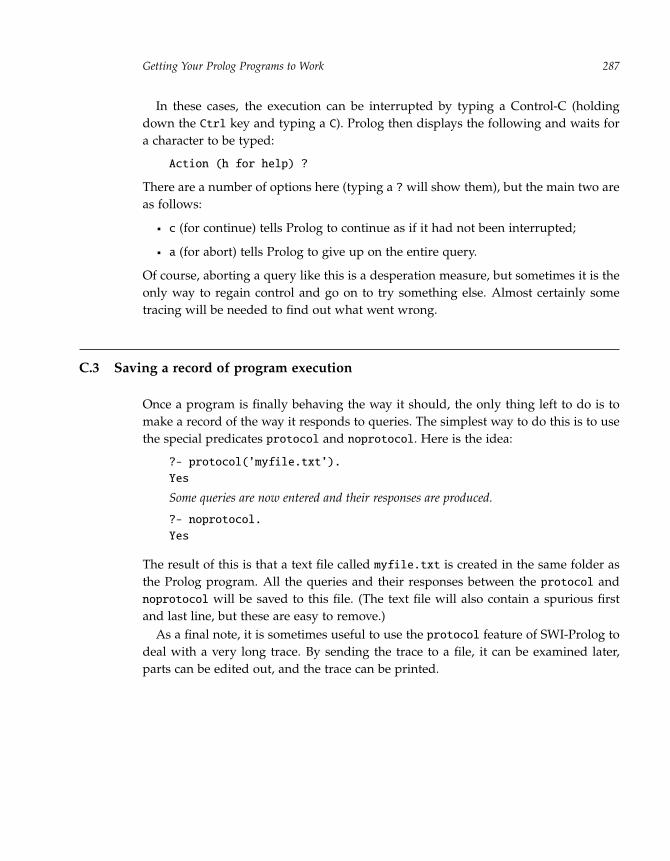
“run” — 2011/9/8 — 18:05 — page 287 — #310�

�

�

�

�

�

�

�

Getting Your Prolog Programs to Work 287

In these cases, the execution can be interrupted by typing a Control-C (holdingdown the Ctrl key and typing a C). Prolog then displays the following and waits fora character to be typed:

Action (h for help) ?

There are a number of options here (typing a ? will show them), but the main two areas follows:

c (for continue) tells Prolog to continue as if it had not been interrupted;

a (for abort) tells Prolog to give up on the entire query.

Of course, aborting a query like this is a desperation measure, but sometimes it is theonly way to regain control and go on to try something else. Almost certainly sometracing will be needed to find out what went wrong.

C.3 Saving a record of program execution

Once a program is finally behaving the way it should, the only thing left to do is tomake a record of the way it responds to queries. The simplest way to do this is to usethe special predicates protocol and noprotocol. Here is the idea:

?- protocol(’myfile.txt’).

Yes

Some queries are now entered and their responses are produced.

?- noprotocol.

Yes

The result of this is that a text file called myfile.txt is created in the same folder asthe Prolog program. All the queries and their responses between the protocol andnoprotocol will be saved to this file. (The text file will also contain a spurious firstand last line, but these are easy to remove.)

As a final note, it is sometimes useful to use the protocol feature of SWI-Prolog todeal with a very long trace. By sending the trace to a file, it can be examined later,parts can be edited out, and the trace can be printed.

“run” — 2011/9/8 — 18:05 — page 288 — #311�

�

�

�

�

�

�

�

“run” — 2011/9/8 — 18:05 — page 289 — #312�

�

�

�

�

�

�

�

Appendix DOther Prolog Systems

There are many implementations of Prolog other than the SWI-Prolog that is usedin this book. Fortunately, many of the more recent systems (including SWI-Prolog,SICStus Prolog, ECLiPSe, and GNU Prolog) use the same ISO Standard Prolog dialect.Variations are found mainly in older systems (such as C-Prolog, Open Prolog, LPAProlog, Quintus Prolog, and Amzi! Prolog). There are many other Prolog systems outthere, however, which can be found by searching online. Each of these systems hasits own advantages and disadvantages regarding special features (including languageadditions), speed of execution, and in some cases, commercial support.

Before talking about language differences, it is worth noting that even in systemsthat use the same dialect of Prolog, the behavior of the systems is not always preciselythe same. It should be possible to run the same queries on the same programs to getthe same answers, but there are variations. For example, in this book, it is assumedthat the system responds to queries by printing Yes (for success) or No (for failure),as it does in release 5.6.43 of SWI-Prolog. But more recent versions of SWI-Prolog,including release 5.6.63, print true or false instead.

This book uses a very small subset of SWI-Prolog. For anyone trying to run theexamples here or write their own programs on a different Prolog system, here aresome things to watch for:

Negation. The symbol \+ is used to indicate negation (see chapter 3, page 49). Manyearlier Prolog systems used the more mnemonic not instead.

Comments. Comments in a Prolog program are indicated with a % and continue tothe end of the line (see chapter 3, page 44). In other Prologs, comments are placedbetween /* and */ characters.

Loading files. Program files are loaded using square parentheses (see appendix B).So the query [myfile] is how the program file myfile.pl is loaded. In otherProlog systems, the query consult(myfile) is used instead.

Reloading files. In SWI-Prolog, if a file is reloaded (using the square brackets or withthe special SWI-Prolog query make introduced in appendix C), the new definitionreplaces the previous one. In other Prologs, new clauses are added to the old ones,unless the special query reconsult is used.

“run” — 2011/9/8 — 18:05 — page 290 — #313�

�

�

�

�

�

�

�

Appendix D290

Dynamic predicates. In SWI-Prolog, predicates are not dynamic unless the special:- dynamic declaration is included in the file (see chapter 8). In some Prologsystems, all predicates are considered to be dynamic. (So if a predicate that doesnot appear in a program is used in a query, the query will fail rather than causean error, as it does in SWI-Prolog.)

Assert and retract. The predicates assert and retract are used here to add andremove clauses for dynamic predicates (see chapter 8). Other Prolog systemsmay use predicates with slightly different names for this purpose.

Member and append. The predicates member and append are built-in predicates inSWI-Prolog. In some older systems, these need to be defined by the user. (Thedefinitions appear in chapter 7 under the names elem and join).

Copying terms. A special predicate copy_term is used in chapter 11. This is a built-in SWI-Prolog predicate, but it is difficult to duplicate otherwise. One definitionthat often works is based on assert and retract:

copy_term(X,Y) :-

assert(mycopy(X)), mycopy(Y), retract(mycopy(X)).

Sending output to a file. The predicates protocol and noprotocol are used to sendthe output produced by Prolog to an external file (see appendix C). Other con-ventions are used in other systems, including tell and told for output, and seeand seen for input.

Tracing. Prolog systems vary considerably on how they handle tracing. The SWI-Prolog conventions are described in appendix C.

There are many tutorials and FAQs about Prolog that can be found online. For moreinformation about SWI-Prolog, see http://www.swi-prolog.org/. A survey that hasa lot of information about many of the older versions of Prolog can be found athttp://www.faqs.org/faqs/prolog/.

“run” — 2011/9/8 — 18:05 — page 291 — #314�

�

�

�

�

�

�

�

References

Chapter 1 Thinking and Computation

[1] Ronald J. Brachman and Hector J. Levesque. Knowledge Representation andReasoning. San Francisco: Morgan Kaufmann, 2004.

[2] Gilles Fauconnier and Mark Turner. The Way We Think: Conceptual Blending andThe Mind’s Hidden Complexities. New York: Basic Books, 2003.

[3] Jerry A. Fodor. The Mind Doesn’t Work That Way. Cambridge, MA: MIT Press,2000.

[4] Frank van Harmelen, Vladimir Lifschitz and Bruce Porter, eds. Handbook ofKnowledge Representation. Amsterdam: Elsevier, 2008.

[5] Philip Johnson-Laird. Mental Models. Cambridge, MA: Harvard UniversityPress, 1986.

[6] Steven M. Kosslyn, William L. Thompson, and Giorgio Ganis. The Case forMental Imagery. Oxford: Oxford University Press, 2009.

[7] Douglas B. Lenat and R. V. Guha. Building Large Knowledge-Based Systems:Representation and Inference in the Cyc Project. Boston: Addison-Wesley, 1990.

[8] Harry Lewis and Christos Papadimitriou. Elements of the Theory of Computation.2d ed. Upper Saddle River, NJ: Prentice Hall, 1997.

[9] Steven Pinker. How the Mind Works. New York: W. W. Norton, 1999.

[10] Zenon W. Pylyshyn. Computation and Cognition: Toward a Foundation for CognitiveScience. Cambridge, MA: MIT Press, 1986.

[11] Stuart J. Russell and Peter Norvig. Artificial Intelligence: A Modern Approach.3d ed. Upper Saddle River, NJ: Prentice Hall, 2009.

[12] Alan Turing. On computable numbers, with an application to the Entschei-dungsproblem. Reprinted in The Undecidable, ed. Martin Davis, 115–153. Mineola,NY: Dover Publications, 2004.

“run” — 2011/9/8 — 18:05 — page 292 — #315�

�

�

�

�

�

�

�

References292

Chapter 2 A Procedure for Thinking

[13] Apostolos Doxiadis and Christos Papadimitriou. Logicomix. New York:Bloomsbury Publishing, 2009.

[14] Herbert B. Enderton. A Mathematical Introduction to Logic. San Diego, CA:Academic Press, 2001.

[15] Elliott Mendelsohn. Introduction to Mathematical Logic. 5th ed. London:Chapman and Hall/CRC, 2009.

Chapter 3 The Prolog Language

[16] Alain Colmerauer and Philippe Roussel. The birth of Prolog. In History ofProgramming Languages, ed. Thomas Bergin Jr. and Richard Gibson Jr., 331–351,New York: ACM Press, 1996.

[17] Carl Hewitt. Planner: A language for proving theorems in robots. In Proceedingsof the International Joint Conference on Artificial Intelligence, Washington, DC, 1969,295–301.

Chapter 4 Writing Prolog Programs

[18] Kenneth A. Bowen. Prolog and Expert Systems Programming. New York: McGraw-Hill, 1991.

[19] Ivan Bratko. Prolog Programming for Artificial Intelligence. 3d ed. Boston:Addison-Wesley, 2000.

[20] William F. Clocksin and Christopher S. Mellish. Programming in Prolog. 4th ed.Berlin: Springer-Verlag, 1994.

[21] Daniel Crookes. Introduction to Programming in Prolog. Englewood Cliffs, NJ:Prentice Hall, 1988.

[22] Tony Dodd. Prolog: A Logical Approach. Oxford: Oxford University Press, 1990.

Chapter 5 Case Study: Satisfying Constraints

[23] Steven A. Cook. The complexity of theorem-proving procedures. In Proceedingsof the Third Annual ACM Symposium on Theory of Computing, Shaker Heights,Ohio, 1971, 151–158.

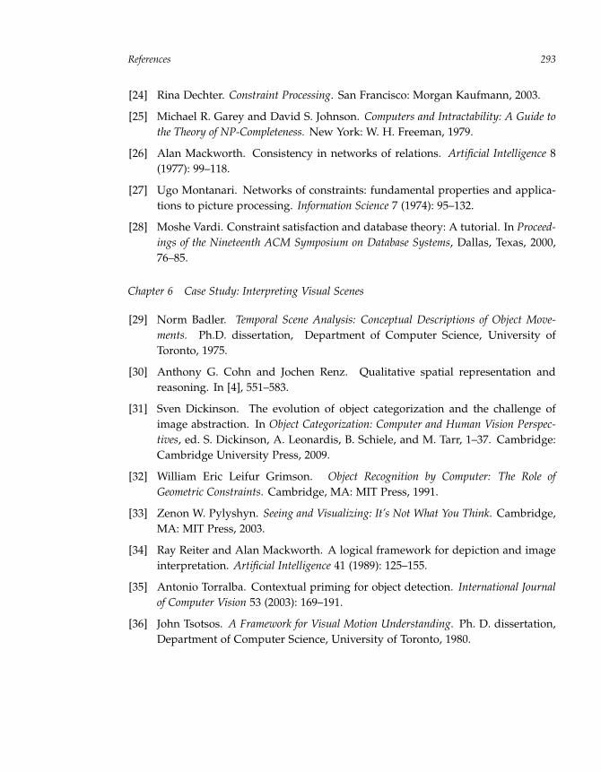
“run” — 2011/9/8 — 18:05 — page 293 — #316�

�

�

�

�

�

�

�

References 293

[24] Rina Dechter. Constraint Processing. San Francisco: Morgan Kaufmann, 2003.

[25] Michael R. Garey and David S. Johnson. Computers and Intractability: A Guide tothe Theory of NP-Completeness. New York: W. H. Freeman, 1979.

[26] Alan Mackworth. Consistency in networks of relations. Artificial Intelligence 8(1977): 99–118.

[27] Ugo Montanari. Networks of constraints: fundamental properties and applica-tions to picture processing. Information Science 7 (1974): 95–132.

[28] Moshe Vardi. Constraint satisfaction and database theory: A tutorial. In Proceed-ings of the Nineteenth ACM Symposium on Database Systems, Dallas, Texas, 2000,76–85.

Chapter 6 Case Study: Interpreting Visual Scenes

[29] Norm Badler. Temporal Scene Analysis: Conceptual Descriptions of Object Move-ments. Ph.D. dissertation, Department of Computer Science, University ofToronto, 1975.

[30] Anthony G. Cohn and Jochen Renz. Qualitative spatial representation andreasoning. In [4], 551–583.

[31] Sven Dickinson. The evolution of object categorization and the challenge ofimage abstraction. In Object Categorization: Computer and Human Vision Perspec-tives, ed. S. Dickinson, A. Leonardis, B. Schiele, and M. Tarr, 1–37. Cambridge:Cambridge University Press, 2009.

[32] William Eric Leifur Grimson. Object Recognition by Computer: The Role ofGeometric Constraints. Cambridge, MA: MIT Press, 1991.

[33] Zenon W. Pylyshyn. Seeing and Visualizing: It’s Not What You Think. Cambridge,MA: MIT Press, 2003.

[34] Ray Reiter and Alan Mackworth. A logical framework for depiction and imageinterpretation. Artificial Intelligence 41 (1989): 125–155.

[35] Antonio Torralba. Contextual priming for object detection. International Journalof Computer Vision 53 (2003): 169–191.

[36] John Tsotsos. A Framework for Visual Motion Understanding. Ph. D. dissertation,Department of Computer Science, University of Toronto, 1980.

“run” — 2011/9/8 — 18:05 — page 294 — #317�

�

�

�

�

�

�

�

References294

[37] David Waltz. Understanding line drawings of scenes with shadows. In ThePsychology of Computer Vision, ed. Patrick Winston, 19–92. New York: McGraw-Hill, 1975.

Chapter 7 Lists in Prolog

[38] John McCarthy. LISP 1.5 Programmer’s Manual. Cambridge, MA: MIT Press,1962.

[39] Leon Sterling and Ehud Shapiro. The Art of Prolog. 2d ed. Cambridge, MA: MITPress, 1994.

Chapter 8 Case Study: Understanding Natural Language

[40] John L. Austin. How to Do Things with Words. 2d ed. Cambridge, MA: HarvardUniversity Press, 1975.

[41] Noam Chomsky. Syntactic Structures. 2d ed. Berlin: Mouton de Gruyter, 2002.

[42] Daniel Jurafsky and James H. Martin. Speech and Language Processing. 2d ed.Upper Saddle River, NJ: Prentice Hall, 2008.

[43] Terry Winograd. Understanding Natural Language. New York: Academic Press,1972.

Chapter 9 Case Study: Planning Courses of Action

[44] Fahiem Bacchus and Froduald Kabanza. Using temporal logic to express searchcontrol knowledge for planning. Artificial Intelligence 116 (2000): 123–191.

[45] Malik Ghallab, Dana Nau, and Paolo Traverso. Automated Planning: Theory andPractice. San Francisco: Morgan Kaufmann, 2004.

[46] Hector J. Levesque and Gerhard Lakemeyer. Cognitive robotics. In [4], 869–886.

[47] John McCarthy. Programs with common sense. Reprinted in Readings inKnowledge Representation, ed. Ronald J. Brachman and Hector J. Levesque. SanFrancisco: Morgan Kaufmann, 1986.

[48] Ray Reiter. Knowledge in Action: Logical Foundations for Specifying and Implement-ing Dynamical Systems. Cambridge, MA: MIT Press, 2001.

“run” — 2011/9/8 — 18:05 — page 295 — #318�

�

�

�

�

�

�

�

References 295

Chapter 10 Case Study: Playing Strategic Games

[49] Michael Genesereth, Nathaniel Love, and Barney Pell. General game playing:Overview of the AAAI competition. AI Magazine 26 (2005): 62–72.

[50] David N. L. Levy and Monroe Newborn. How Computers Play Chess. New York:W. H. Freeman, 1990.

[51] Martin Muller. Computer Go. Artificial Intelligence 134 (2002): 145–179.

[52] Jonathan Schaeffer, Neil Burch, Yngvi Bjornsson, Akihiro Kishimoto, MartinMuller, Rob Lake, Paul Lu and Steve Sutphen. Checkers is solved. Science 317(2007): 1518–1522.

Chapter 11 Case Study: Other Ways of Thinking

[53] Harold Abelson and Gerald Jay Sussman. Structure and Interpretation of ComputerPrograms. Cambridge, MA: MIT Press, 1996.

[54] Marc Denecker and Antonis Kakas. Abduction in logic programming. In Com-putational Logic: Logic Programming and Beyond, 402–437. LNAI 2407. Berlin:Springer Verlag, 2002.

[55] Carla P. Gomes, Henry Kautz, Ashish Sabharwal, and Bart Selman. Satisfiabilitysolvers. In [4], 89–134.

[56] Nada Lavrak and Saso Dzeroski. Inductive Logic Programming: Techniques andApplications. Chichester, UK: Ellis Horwood, 1994.

[57] Larry Wos, Ross Overbeek, and Ewing Lusk. Automated Reasoning: Introductionand Applications. Englewood Cliffs, NJ: Prentice Hall, 1984.

Chapter 12 Can Computers Really Think?

[58] Daniel C. Dennett. Consciousness Explained. Boston: Little, Brown, 1991.

[59] Paul Edwards, ed. The Encyclopedia of Philosophy. New York: Macmillan, 1967.

[60] Jerry A. Fodor. The Language of Thought. Cambridge, MA: Harvard UniversityPress, 1975.

[61] Hector J. Levesque. Is it enough to get the behavior right? In Proceedings ofthe Twenty-First International Joint Conference on Artificial Intelligence, Pasadena,California, 2009, 1439–1444.

“run” — 2011/9/8 — 18:05 — page 296 — #319�

�

�

�

�

�

�

�

References296

[62] John R. Lucas. Minds, machines, and Godel. Reprinted in Minds and Machines,ed. Alan Ross Anderson, 43–59. Englewood Cliffs, NJ: Prentice-Hall, 1964.

[63] Roger Penrose. The Emperor’s New Mind: Concerning Computers, Minds, and theLaws of Physics. Oxford: Oxford University Press, 1989.

[64] John Searle. Minds, brains and programs. Behavioral and Brain Sciences 3 (1980):417–424.

[65] Brian C. Smith. The owl and the electric encyclopaedia. Artificial Intelligence 47(1991): 251–288.

[66] Alan Turing. Computing machinery and intelligence. Mind 59 (1950): 433–460.

“run” — 2011/9/8 — 18:05 — page 297 — #320�

�

�

�

�

�

�

�

Index of Technical Terms

These are the main technical terms presented in the book. They are introducedat the page number indicated, where the words appear underlined.

* (multiplication), 97** (exponentiation), 97+ (addition), 97- (subtraction), 97/ (division), 97// (integer quotient), 99:- (conditional operator), 44; (query command), 47< (less than), 97= (equal), 53=:= (numerically equal), 97=< (less than or equal), 97> (greater than), 97>= (greater than or equal), 97?- (query prompt), 45% (start of a comment), 44| (list head and tail separator), 139\+ (negation), 49_ (anonymous variable), 91

abduction, 239action precondition clause, 202algorithm, 79alpha cutoff, 232ambiguity (in a grammar), 158anonymous variable, 91append predicate, 145argument of a predicate, 43arithmetic expression, 97arithmetic relation, 97assert predicate, 172atom, 43atomic sentence (in Prolog), 43

back-chaining, 27backtracking, 33beta cutoff, 232body of a clause, 44breadth-first procedure, 244

classification, 256clause, 44CNF, 258comment (in Prolog), 44computation, 5conditional sentence (in Prolog), 44conjunctive normal form, 258conjunctive query, 48constant (in Prolog), 43constraint (in constraint satisfaction), 89constraint satisfaction problem, 89copy_term predicate, 247correctness of a program, 66

dclause (disjunctive clause), 258deduction, 239Deep Blue, 232depth-first procedure, 244domain (in constraint satisfaction), 89dynamic (Prolog declaration), 172dynamic predicate, 172

element of a list, 138empty list, 138entailment, see logical entailmentequality query, 53establishing a query, 27explanation, 239

“run” — 2011/9/8 — 18:05 — page 298 — #321�

�

�

�

�

�

�

�

Index of Technical Terms298

final state of a game, 211fluent, 199forward-chaining, 36

game tree, 213generate-and-test, 86goal state, 182goal-directed reasoning, 36grammar, 156

halt predicate, 45head of a clause, 44head of a list, 138

induction, 240initial state, 182, 211initial state clause, 200input of a procedure, 5instantiated variable, 53is (variable equality), 97

knowledge base (KB), 19knowledge-based system, 19

labeling a game tree, 213language processor, 249learning, 240leash predicate, 286legality of a move, 182, 211lexicon, 155list, 138literal, 55logical completeness, 36logical correctness of a program, 65logical entailment, 15, 25logical soundness, 36ls predicate, 284

make predicate, 284

mathematical induction, 69member predicate, 145minimax, 228mod (integer remainder), 99

negated query, 49nl (newline) predicate, 90noprotocol predicate, 287number (in Prolog), 96numerical game tree, 227

once predicate, 257operator of a planning problem, 182output of a procedure, 5

parsing, 157plan, 182player in a game, 211predicate (in Prolog), 43procedure, 5program (in Prolog), 44proposition, 13propositional language, 258propositional reasoning, 240protocol predicate, 287

query, 24query (in Prolog), 46quoted-string, 43

reachability of a state, 183read predicate, 221recursion, 60, 68retract predicate, 172

satisfiability of sentences, 259search space, 94situation, 198solution (in constraint satisfaction), 89

“run” — 2011/9/8 — 18:05 — page 299 — #322�

�

�

�

�

�

�

�

Index of Technical Terms 299

split_words predicate, 170state of a planning problem, 182successor state clause, 200symbol, 4symbolic structure, 5

tail of a list, 138term, 55, 139test example, 256trace predicate, 286trace (in Prolog), 51tracing a procedure, 28training example, 256

unification, 56uninstantiated variable, 53

variable (in constraint satisfaction), 89variable (in Prolog), 43

web of belief, 17write predicate, 90

Documents

Thinking as Computation