1

THESIS

THE EFFECTS OF LONG TERM NITROGREN FERTILIZATION ON FOREST SOIL

RESPIRATION IN A SUBALPINE ECOSYSTEM IN ROCKY MOUNTAIN NATIONAL

PARK

Submitted by

Jordan Allen

Graduate Degree Program in Ecology

Impartial fulfillment of the requirements

For the Degree of Master of Science

Colorado State University

Fort Collins, Colorado

Spring 2016

Master’s Committee: Advisor: A. Scott Denning Co-Advisor: Jill Baron Mike Ryan

Gillian Bowser

2

ABSTRACT

EFFECTS OF NITROGREN FERTILIZATION ON FOREST SOIL RESPIRATION IN A

SUBALPINE ECOSYSTEM IN ROCKY MOUNTAIN NATIONAL PARK

Anthropogenicactivitiescontributetoincreasedlevelsofnitrogendepositionand

elevatedCO2concentrationsinterrestrialecosystems.Theresponseofsoilrespirationto

nitrogenfertilizationinanongoing18-yearfieldnitrogenamendmentstudywas

conductedfromJuly2014toOctober2014.Thefocusofthisstudywastodeterminethe

effectsofnitrogenfertilizationonsoilcarboncycling,viarespiration.Ourobjectiveswere

to(1)testthehypothesisthatNadditionswouldincreasesoilrespirationinNsaturated

subalpineforests,and(2)try to understand the impacts of N additions on carbon flows in the

ecosystem.ALiCor LI-820 infrared gas analyzer (IRGA) was used to quantify soil respiration

rates. WecomparedsoilCO2respirationfromfertilizedforestplots(30x30m)withCO2

respirationfromcontrolforestsplots(30x30m)thatreceiveonlyambientnitrogen

deposition(3-5 kg/ N/ha-1/yr-1) during the2013-growingseason.Ourresultsshowthatmean

soilrespirationmeasurementswerenotsignificantlydifferentinthecontrolplots(3.14

µmol m-2 sec-1) thaninthefertilizedplots(3.02 µmol m-2 sec-1).

Experimentswithaverysimpleecosystemmodelsuggestthatthenegligible

responseofsoilrespirationinthefertilizedvscontrolplotsisaresultofnitrogen

saturationduetoatmosphericdepositionofN.

Interestingly,theQ10functionusedtoestimatethetemperaturesensitivitywas

2.06ºC forevery8.1µmol m-2 sec-1 (R0)inthecontrolplotscomparedto1.73ºC forevery

6.3µmol m-2 sec-1 (R0)inthefertilizedplots,indicatingthatthetemperaturefunctionis

3

slightlyhigherinthecontrolplots.Treatmentwasinsignificantininfluencingsoil

respiration(p-valuegreaterthan0.5).TheSimpleEcosystemModelwasusedtosimulate

theoutputfromland-atmosphereinteractionwiththesensitivityofNetprimary

production(NPP)andrespirationinresponsetonutrients.Ourresultssuggeststhe

effectsofnitrogenfertilizationonsoilrespirationinRockyMountainNationalPark

insignificantlyinfluencechangesinsoilrespirationtoambientatmosphericNdepositionin

subalpineforests.

4

ACKNOWLEDGEMENTS

As I embarked on this journey to pursue graduate education at Colorado State University.

My goals were to develop as a scholar, work with a collaborative/interdisciplinary research

group, ultimately finish and pursue a career in science. I really appreciate the guidance and

mentorship from my committee Dr. A. Scott Denning, Dr. Jill Baron, Dr. Mike Ryan and Dr.

Gillian Bowser. I am grateful for your support. I also, would like to thank Daniel Bowker for

helping me throughout my field season. Most importantly, I would like to thank my family and

friends for their continuous support throughout my pursuit of continuing my education.

Lastly, the National Science Foundation under Award Number 0425247 Center for

Multiscale Modeling of Atmospheric Processes (CMMAP) funded this research.

5

TABLE OF CONTENTS

ABSTRACT ............................................................................................................................... ii

ACKNOWLEDGEMENTS ....................................................................................................... iv

INTRODUCTION ...................................................................................................................... 5

METHODS ............................................................................................................................... 10

RESULTS ................................................................................................................................. 20

CONCLUSION......................................................................................................................... 27

REFERENCES ......................................................................................................................... 29

6

1. Introduction

Since the Industrial Revolution, nitrogen (N) deposition has increased at an alarming rate

(Hoberg, 2007). Nitrogen deposition is defined as the input of reactive nitrogen species from the

atmosphere to the biosphere. The pollutants that contribute to nitrogen deposition derive mainly

from nitrogen oxides (NOX) and ammonia (NH3) emissions and impact terrestrial ecosystems

(Fenn et al. 2003). Due to anthropogenic activities atmospheric nitrogen fixed annually through

human activities now exceeds that fixed via all natural processes combined (Neff et al. 2002).

Nitrogen is deposited in ecosystems in gaseous, dissolved and particulate forms. Deposition

occurs by three processes: (1) Wet deposition from precipitation, which delivers dissolved

nutrients; (2) Dust or aerosols by sediments known as dry deposition; and (3) Cloud-water

deposition delivers nutrients in water droplets onto plant surfaces (Chaplin et al 2010). The form

of nitrogen deposition determines its ecosystem consequences (Vitousek et al. 1997).

Anthropogenic activities are the main causes of nitrogen deposition (Gruber and Galloway

2008). Due to high use of fertilizer agricultural systems are often nitrogen saturated and release

substantial quantities of nitrogen to ecosystems. Some boreal and temperate forests increase their

carbon sequestration in response to nitrogen deposition (Magnani et al. 2007).

The Colorado Front Range population growth, land use change and agricultural practices

have increased pollution and specifically nitrogen deposition. The main sources of pollutants are

power plants, vehicles, agriculture fertilizers and livestock (Baron et al. 2004). In the Rocky

Mountain region, upslope winds from the east are transporting and depositing nitrogen. During

weather events, reactive nitrogen is transported by wind, combined with moisture in the air and

then deposited by precipitation (Wolyn and Mckee 1994, Markowski and Richardson 2010).

Many studies have highlighted the effects of anthropogenic nitrogen deposition in ecosystems

7

(Agren et al. 1988; Asner et al. 1997; Currie et al. 1999), but most importantly in the Colorado

Front Range, Baron et al. (2000) have found that slight increases in nitrogen deposition led to

changes in ecosystem properties. Biological systems such as lakes, trees, and microbes in pristine

mountain systems are influenced by excess nitrogen deposition (Williams et al. 2000; Friedland

et al.1991).

Nitrogen deposition may cause soil to respire more CO2 (Janssens et al. 2010). The rate

of carbon storage has to increase or change at a dramatic rate for change. Small changes in large

pools of carbon can have a dramatic impact on the CO2 content of the atmosphere, if they are not

balanced by simultaneous changes in other components of the carbon cycle (Pan et al. 2010).

Annual emissions of anthropogenic CO2 in the atmosphere has increased at an alarming rate due

to the combustion of fossil fuels (Freidlingstein et al. 2010). The increase in CO2 alters the

carbon sinks such as the land, oceans, and the atmosphere. One of the main causes of global

warming is increased carbon dioxide CO2 in the atmosphere. The atmospheric concentration of

CO2 has increased from its preindustrial levels, about 280 parts per million (ppm), to 400 ppm

(Mauna Loa Observatory). Nadelhoffer et al. 1999 found that nitrogen deposition makes a small

contribution to carbon sequestration in temperate forests, but there is still uncertainty whether

elevated nitrogen deposition is the main cause.

The global flux of CO2 from soils is approximately 75 x 1015 gC/yr (Schlesinger, 1997).

Waldrop et. al, 2004 found nitrogen deposition alters carbon cycling in soils and influences

changes in microbial activity. In our study we are focusing on the effects of nitrogen fertilization

on forest soil respiration in Rocky Mountain National Park. The role of soil in biogeochemical

cycles is an important area of uncertainty in ecosystem ecology. One of the main reasons for this

uncertainty is that we have a limited understanding of belowground microbial activity and how

8

this activity is linked to soil processes. Soil respiration is the one of the most important

components of ecosystem respiration. It is linked to photosynthesis, litter fall and plant

metabolism because of belowground activity by both autotrophic and heterotrophic activity

(Ryan 1991). Autotrophic respiration is defined as root growth and rhizo-microbial respiration.

Heterotrophic is defined as litter, labile soil organic matter and stable soil organic matter. It is

still very much uncertain why some soil organic matter persists for a long period of time and

some decomposes fast (Schmidt 2003).

In this study our goal is to understand the effects of long-term nitrogen deposition on

forest soil respiration in Rocky Mountain National Park. Primary production by forest

ecosystems is usually nitrogen limited, meaning that adding nitrogen causes an increase in

photosynthesis. We therefore expect that deposition of anthropogenic reactive nitrogen in Rocky

Mountain National Park will lead to increased photosynthesis and greater carbon storage in

biomass and litter. Over time, increased carbon storage in litter and soils should lead to increased

respiration from forest soils. To test this hypothesis, we measured soil respiration in forest plots

that had been fertilized for 18 years, and compared the results to control plots that received only

ambient nitrogen deposition. Chapter 2 describes the experimental site, methods, and

calculations. Chapter 3 presents results of the measurements and some numerical experiments

with a simple ecosystem model. Chapter 4 discusses the results, summarizes our conclusions,

and offers some ideas for future work.

9

2. Methods

2.1 Site Description

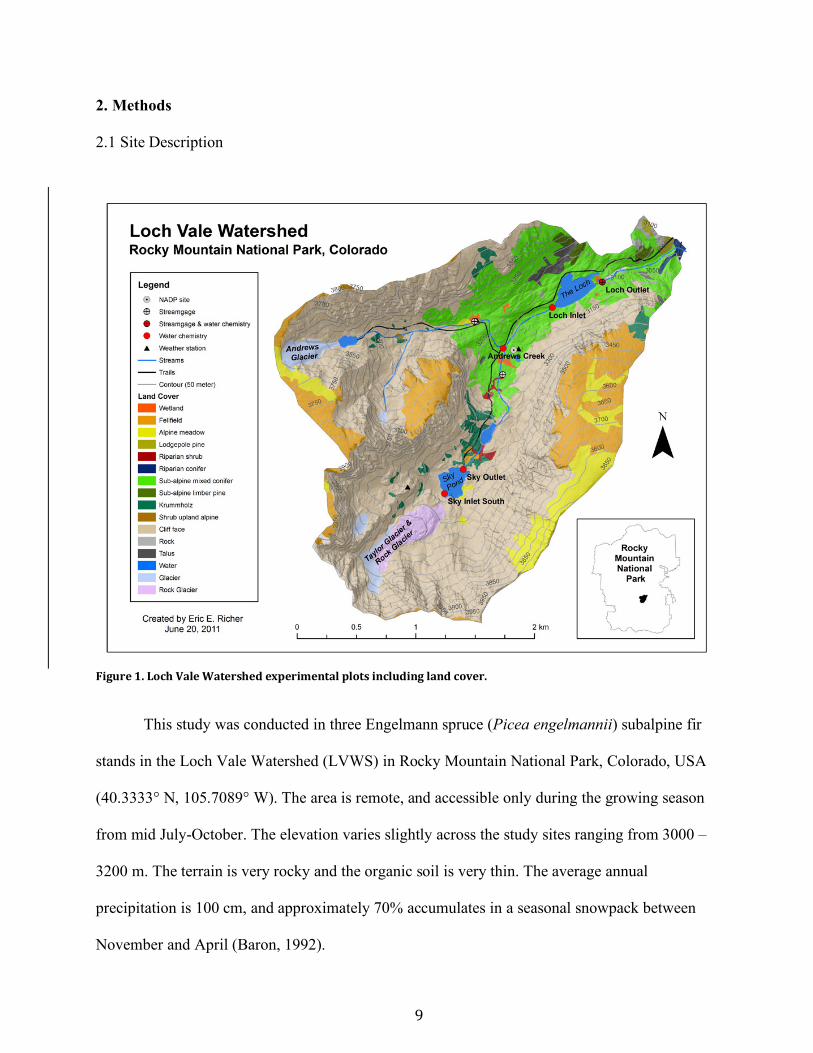
Figure1.LochValeWatershedexperimentalplotsincludinglandcover.

This study was conducted in three Engelmann spruce (Picea engelmannii) subalpine fir

stands in the Loch Vale Watershed (LVWS) in Rocky Mountain National Park, Colorado, USA

(40.3333° N, 105.7089° W). The area is remote, and accessible only during the growing season

from mid July-October. The elevation varies slightly across the study sites ranging from 3000 –

3200 m. The terrain is very rocky and the organic soil is very thin. The average annual

precipitation is 100 cm, and approximately 70% accumulates in a seasonal snowpack between

November and April (Baron, 1992).

10

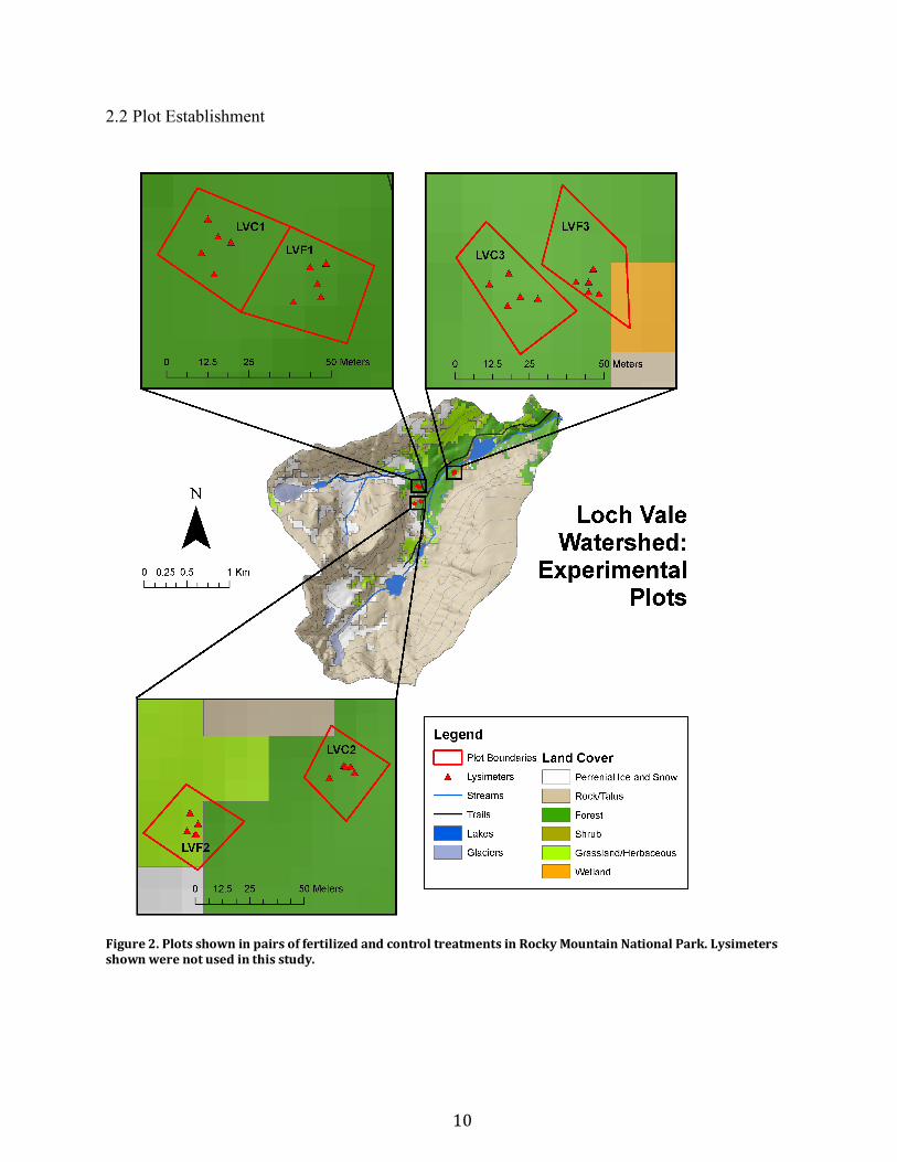
2.2 Plot Establishment

Figure2.PlotsshowninpairsoffertilizedandcontroltreatmentsinRockyMountainNationalPark.Lysimetersshownwerenotusedinthisstudy.

11

A total of six 30 x 30 m plots were established in June 1996. Pairs of adjacent plots

(Figure 2) are fertilized (LVF1, LVF2, LVF3) and control (LVC1, LVC2, LVC3). Fertilized

plots received 25 kg N ha-1 yr-1 as ammonium nitrate (NH4NO3) pellets, while control plots

received only ambient atmospheric nitrogen deposition of 3 to 5 kg N ha-1 yr-1 (Rueth et al.,

2003). Plots were accessed in the summer using hiking trails.

2.3 Procedure

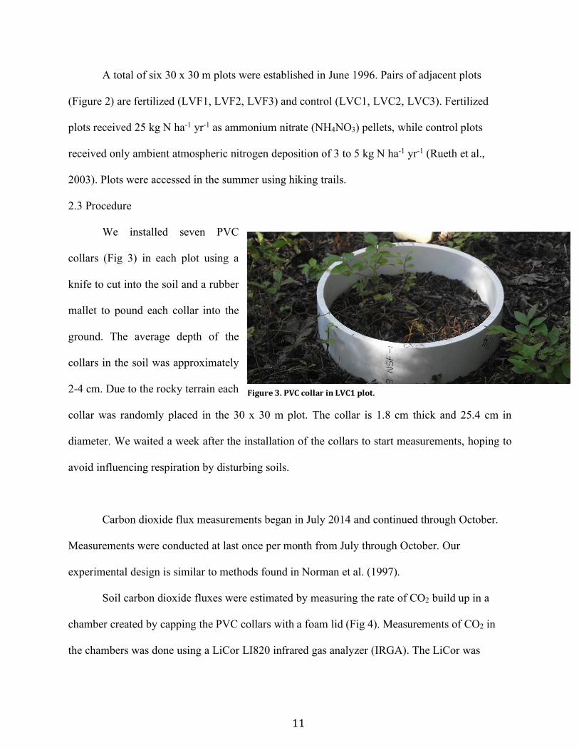
We installed seven PVC

collars (Fig 3) in each plot using a

knife to cut into the soil and a rubber

mallet to pound each collar into the

ground. The average depth of the

collars in the soil was approximately

2-4 cm. Due to the rocky terrain each

collar was randomly placed in the 30 x 30 m plot. The collar is 1.8 cm thick and 25.4 cm in

diameter. We waited a week after the installation of the collars to start measurements, hoping to

avoid influencing respiration by disturbing soils.

Carbon dioxide flux measurements began in July 2014 and continued through October.

Measurements were conducted at last once per month from July through October. Our

experimental design is similar to methods found in Norman et al. (1997).

Soil carbon dioxide fluxes were estimated by measuring the rate of CO2 build up in a

chamber created by capping the PVC collars with a foam lid (Fig 4). Measurements of CO2 in

the chambers was done using a LiCor LI820 infrared gas analyzer (IRGA). The LiCor was

Figure3.PVCcollarinLVC1plot.

12

connected to a Campbell Scientific data logger, which was programmed to record CO2

concentrations every two seconds in air pumped in a tube from the IRGA to the chamber open

only to the soil in the collar. The IRGA was roughly calibrated before each measurement using

400 ppm CO2 as the ambient air standard. To make sure these flux measurements are not biased

by CO2 concentration gradients between the chamber and the air, we scrubbed the concentration

within the chamber down to just below ambient CO2 concentration using a second airflow tube

to pump the air from the chamber through a soda lime trap. Soil respiration then causes the

concentration to build up again and we measure the rate of change in concentration close to

ambient levels. Linear regressions (concentration versus time) were used to determine rates of

CO2 flux. Soil CO2 flux in µmol m-2 sec-1 was obtained by taking the slope of the line of CO2

concentration (parts per million) as a function of time, and multiplying it by the volume of the

chamber divided by its surface area, correcting for temperature and pressure to obtain respiration

flux in moles m-2 s-1 (see section 2.5 below). The rate of CO2 build up was almost perfectly

linear. Air temperature was measured at one location near the three pairs of plots and soil

temperature and moisture was measured near each collar. Measurements were conducted during

the growing season between the dates of July 21 and October 20 in 2014.

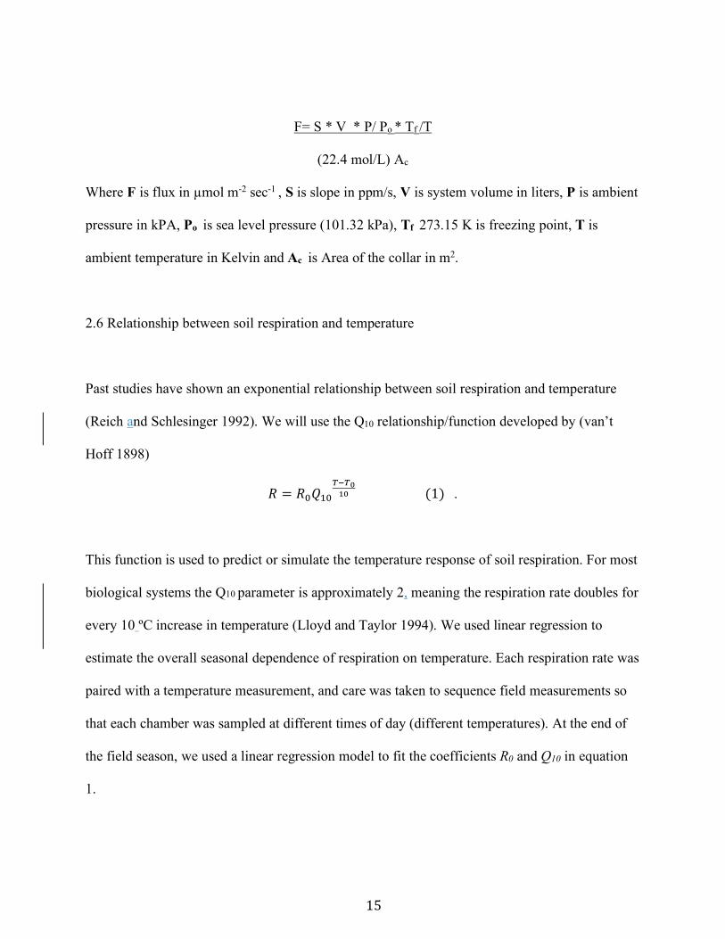
2.4 Full sampling cycle using LiCOR and soil collar:

1) User initiates start – air flows through soda lime trap

2) Scrubbing of [CO2] ppm until it is below Lower Boundary Sampling Level

3) Air flows through IRGA for duration of user determined Lag Time and until [CO2] is

above Lower Boundary Sampling Level

13

4) Datalogger records a sample every two seconds during the Sampling Time for flux

calculations.

5) Sampling record terminates.

6) Datalogger sends new data to storage module.

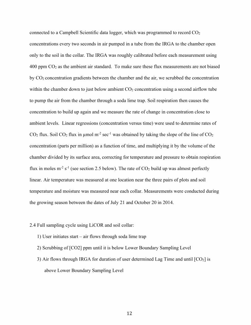
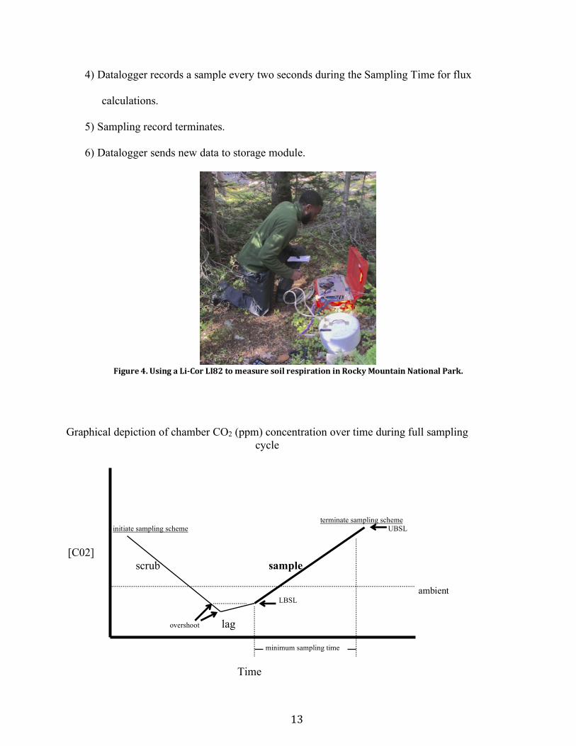
Figure4.UsingaLi-CorLI82tomeasuresoilrespirationinRockyMountainNationalPark.

terminate sampling scheme initiate sampling scheme UBSL [C02] scrub sample ambient LBSL overshoot lag

minimum sampling time Time

Graphical depiction of chamber CO2 (ppm) concentration over time during full sampling cycle

14

2.5 Flux Calculations

• System + tubing = 50 cm3 = 0.05 L

• Collar area (m2): 10" diameter = 506.7075 cm2 = 0.050671 m2

• Chamber Volume = 5.365 cm3 (inside LiCor)

(Collar Area (in cm3) multiplied by the Collar Depth) plus Chamber Volume plus System

plus Tubing (in cm3)

Collar 5 cm deep: (506.7075 * 5) + 5365 + 50 = 7948.5 cm3 or 0.0079485 m3. Flux = increase in CO2/ time * volume / surface area

• The increase in CO2 / time = slope

Conversion of CO2 increase to soil respiration

Flux = slope µmol CO2 mol Air-1 s-1 (slope of regression of CO2 ppm versus time)

*(103 L/m3) * (system volume in m3) * (1 mol/22.414 L) * (Pressure in kPa/101.32 kPa) *

(From Licor gas analyzer/Standard pressure of 101.32 kPa) *(273 °K/Air temperature in

°K) 1/ 0.050671 m2).

F = Flux

S = Slope

Vs = Volume of System

P = Ambient pressure

Po = Standard Pressure (Sea level)

Tf = 273.15 K

T = Temperature from National Atmospheric Deposition Program National Trends Network

(NADP/NTN) monitors

Ac = Area of Collar

15

F= S * V * P/ Po * Tf /T

(22.4 mol/L) Ac

Where F is flux in µmol m-2 sec-1 , S is slope in ppm/s, V is system volume in liters, P is ambient

pressure in kPA, Po is sea level pressure (101.32 kPa), Tf 273.15 K is freezing point, T is

ambient temperature in Kelvin and Ac is Area of the collar in m2.

2.6 Relationship between soil respiration and temperature

Past studies have shown an exponential relationship between soil respiration and temperature

(Reich and Schlesinger 1992). We will use the Q10 relationship/function developed by (van’t

Hoff 1898)

𝑅 = 𝑅#𝑄%#&'&()( (1).

This function is used to predict or simulate the temperature response of soil respiration. For most

biological systems the Q10 parameter is approximately 2, meaning the respiration rate doubles for

every 10 ºC increase in temperature (Lloyd and Taylor 1994). We used linear regression to

estimate the overall seasonal dependence of respiration on temperature. Each respiration rate was

paired with a temperature measurement, and care was taken to sequence field measurements so

that each chamber was sampled at different times of day (different temperatures). At the end of

the field season, we used a linear regression model to fit the coefficients R0 and Q10 in equation

1.

16

2.7 Soil moisture and temperature measurements

Soil temperature and moisture were taken at each collar while soil respiration was being

measured. Soil Temperature was initially measured using a Penetration Thermocouple Probes

“T” style 304 stainless steel handle. We inserted the temperature probe 10 cm in depth in soil,

but it did not work. Instead we used hourly measurements of air temperature, which were taken

at the National Atmospheric Deposition Program National Trends Network (NADP/NTN)

monitors a few hundred meters away from the experimental plots. Soil moisture was measured

with a hand held Hydrosense time domain reflectometer (TDR) probe that measured soil

moisture in percent volumetric water content (VWC).

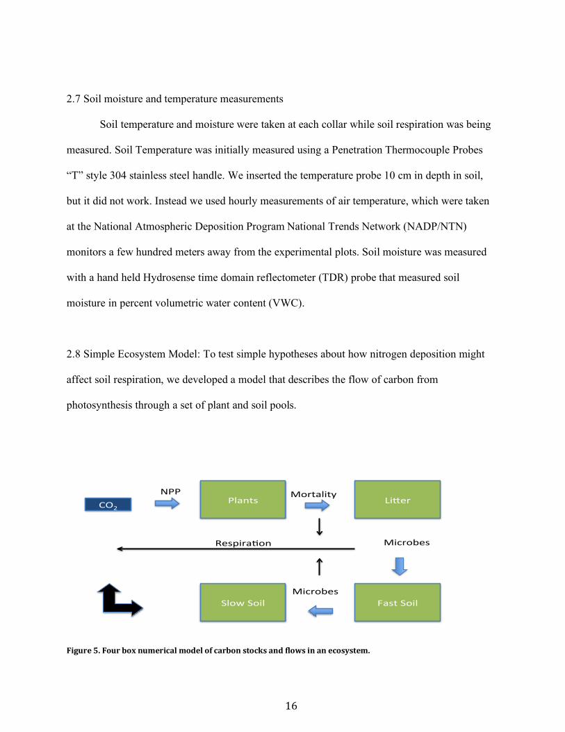
2.8 Simple Ecosystem Model: To test simple hypotheses about how nitrogen deposition might

affect soil respiration, we developed a model that describes the flow of carbon from

photosynthesis through a set of plant and soil pools.

CO2$

Fast$Soil$Slow$Soil$

Plants$ Li1er$NPP$ Mortality$

Microbes$

Microbes$

Respira;on$

Figure5.Fourboxnumericalmodelofcarbonstocksandflowsinanecosystem.

17

We used four boxes to represent storage of carbon in organic matter (Figure 5). Carbon

transfersamongthepoolsarerepresentedasa“cascade”fromonepooltothenext.

Photosynthesis converts CO2 to plants (P), and is limited by nitrogen. Plant mortality (death)

converts plant carbon to “litter,” (L) which is slowly decomposed by microbes to produce fast-

turnover soil organic matter (F). Fast soil is decomposed more slowly by other microbes to

produce slowly-decomposing soil organic matter (S), which will eventually decompose back to

CO2. The model was implemented in R, and the code is presented in the Appendix.

1

2

3

4

Lossesfromeachpoolarerepresentedassourcesofcarbontothenextpool.Carbon

turnoverfromlitter,fastsoilorganicmatterandslowsoilorganicmatterisrepresented

usingturnovertimes( and ).Microbialtransformationsfromlittertofastsoil,

andfromfasttoslowsoilorganicmatterareincompleteduetorespirationlosses.We

representthemetabolicefficiencyofthesemicrobialtransfersase,meaningthatafraction

eofthecarbonlostfromthelitterandfastsoilpoolsisrespiredawayasCO2,withthe

remainingfraction(1- e)beingtransferredtothenextpoolinthecascade.

Toinvestigatetheeffectsofnitrogenfertilizationonsoilrespiration,weexperimentedwith

thesimpleecosystemcarbonmodeldescribedinSection2.8

dPdt

= NPP −mort

dLdt

= mort − Lτ L

dFdt

= (1−ε) Lτ L

−Fτ L

dSdt

= (1−ε) Fτ F

−Sτ S

τ L , τ F , τ S

18

Ecosystemnetprimaryproductionwasrepresentedusingalogisticfunction

5

wheregistherateofintrinsicgrowth(unitless),Pisthecarbonstoredinplants(kgCm-2),

andKisthe“carryingcapacity”oftheecosystem(kgCm-2).

WerepresenttheeffectofnitrogenfertilizationbymodifyingthecarryingcapacityKas

follows

6

HereK0isareferencecarryingcapacity,andNrepresentstheeffectofaddednitrogen.For

convenience,wealsointroduceanitrogen“multiplier”mNwhichcanbeusedtoadjustthe

relativestrengthofthenitrogeneffect.

Mortalityisrepresentedas

7

meaningthattherateoftransferofcarbontothelitterpoolishalftherateofgrowthof

plantcarbon.

Werepresentedahypotheticaleffectofnitrogenonsoilrespirationas

8

Forthesimulationsshownhere,weusee=0.8,tL=2yr,tF=20yr,andtS=500yr.The

modelwasinitializedbysettingthetimederivativesontheleft-handsidesofequations(1)

–(4)tozeroandsolvingforsteady-statevaluesofthecarbonpoolsP,L,F,andS.

We created two sets of experiments because we wanted to predict the response of respiration and

NPP = g 1−PK

⎛

⎝⎜

⎞

⎠⎟P

K = K0 (1+N mN )

mort = g2P

R = εLτ L

+Fτ F

⎛

⎝⎜

⎞

⎠⎟+

Sτ S

⎡

⎣⎢

⎤

⎦⎥(1+N mR )

19

NPP to nutrient additions.

K = K0 (1 + N x multiplier)

N= 0.20 Nutrient concentration

1. Let nutrients increase over a 20-year period.

• Hold the npp/resp multiplier at 0. • Increase npp and resp multiplier. • Decrease npp and increase resp multiplier

2. Hold nutrients constant over a 20 year period • Hold the npp/resp multiplier at 0. • Increase npp and resp multiplier. • Decrease npp and increase resp multiplier

2.9StatisticalAnalysis

LinearregressionanalysiswasperformedusingRstatisticalsoftwareversion

3.0.1(RCoreTeam.2012).Ianalyzedrespirationasafunctionoftreatment,soilmoisture,

soiltemperatureandinteractionsacrossdatacollectedfromallplotsduringthefield

season.Theeffectofsoilmoistureandtemperatureonsoilcarbonfluxwasevaluatedusing

thesefactorsascovariatestotheeffectoffertilization.

20

3.Results

3.1SoilTemperatureandMoisture

Thecomparisonofcontrolandfertilizedplotsrespirationratesinresponsetotemperature.

Soilrespiration,temperature,andmoisturewerestatisticallyidenticalbetween

fertilizedandcontrolplotsovertheentiresummer(Fig6).Duringourfieldseasonthe

meansoiltemperatureforthecontrolplotswere11.09°Candthefertilizedplotswas

approximately11.15°C.Thefluxmeasurementswereaslightlyhigherinthecontrolplots

atapproximately3.14µmolm-2sec-1comparedto3.02µmolm-2sec-1inthefertilizedplots.

Soilmoisturewasverysimilarin

boththefertilizedandcontrol

plots0.29and0.28percent.

Figure6.Comparisonofsoilrespiration,temperatureandmoisturebetweentreatments.Blue=Control,Red=Fertilized

21

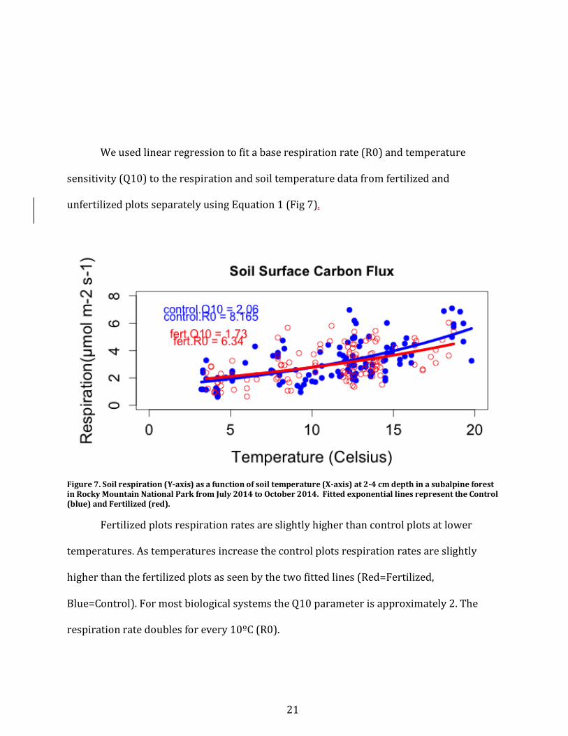
Weusedlinearregressiontofitabaserespirationrate(R0)andtemperature

sensitivity(Q10)totherespirationandsoiltemperaturedatafromfertilizedand

unfertilizedplotsseparatelyusingEquation1(Fig7).

Figure7.Soilrespiration(Y-axis)asafunctionofsoiltemperature(X-axis)at2-4cmdepthinasubalpineforestinRockyMountainNationalParkfromJuly2014toOctober2014.FittedexponentiallinesrepresenttheControl(blue)andFertilized(red).

Fertilizedplotsrespirationratesareslightlyhigherthancontrolplotsatlower

temperatures.Astemperaturesincreasethecontrolplotsrespirationratesareslightly

higherthanthefertilizedplotsasseenbythetwofittedlines(Red=Fertilized,

Blue=Control).FormostbiologicalsystemstheQ10parameterisapproximately2.The

respirationratedoublesforevery10ºC(R0).

22

ThebaserespirationrateR0wasslightlyhigher8.2µmolm-2sec-1inthecontrolvs.the

fertilizedplots6.3µmolm-2sec-1.ThetemperaturesensitivityparameterQ10washigher

(2.06)inthecontrolplotscomparedtothefertilizedplots(1.73).

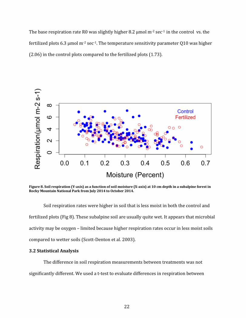
Figure8.Soilrespiration(Y-axis)asafunctionofsoilmoisture(X-axis)at10cmdepthinasubalpineforestinRockyMountainNationalParkfromJuly2014toOctober2014.

Soilrespirationrateswerehigherinsoilthatislessmoistinboththecontroland

fertilizedplots(Fig8).Thesesubalpinesoilareusuallyquitewet.Itappearsthatmicrobial

activitymaybeoxygen–limitedbecausehigherrespirationratesoccurinlessmoistsoils

comparedtowettersoils(Scott-Dentonetal.2003).

3.2StatisticalAnalysis

Thedifferenceinsoilrespirationmeasurementsbetweentreatmentswasnot

significantlydifferent.Weusedat-testtoevaluatedifferencesinrespirationbetween

23

controlandfertilizedplots.Themeasurementswerenotsignificantlydifferent,p-valuewas

greaterthan0.5.Forstatisticalsignificanceatthe95%confidencelevel,weneedp<0.05.

1.Formulalm(flux~treatment)Residuals:Min1QMedian3QMax-2.5295-0.9700-0.18230.82663.9415Coefficients:EstimateStd.ErrortvaluePr(>|t|)(Intercept)3.14120.126824.771<2e-16***treatmentFertilized-0.11690.1817-0.6430.521Residualstandarderror:1.377on228degreesoffreedomMultipleR-squared:0.001811, AdjustedR-squared:-0.002567F-statistic:0.4137on1and228DF,p-value:0.5207

Weusedat-testtoevaluatedifferencesinrespirationbetweentemperatures.The

measurementsshowthattemperatureisamajorfactorinrespirationrates.Thep-value:<

2.2e-16.

Formula1.2:lm(flux~temp)Residuals:Min1QMedian3QMax-2.1898-0.8569-0.13900.83803.6595Coefficients:EstimateStd.ErrortvaluePr(>|t|)(Intercept)0.940440.213024.4151.56e-05***temp0.192700.0179510.734<2e-16***Residualstandarderror:1.124on228degreesoffreedomMultipleR-squared:0.3357, AdjustedR-squared:0.3328F-statistic:115.2on1and228DF,p-value:<2.2e-16

24

1.3Formulalm(flux~moisture)Weusedat-testtoevaluatedifferencesinrespirationbetweenmoisture.The

measurementsshowthatmoisturewasamajorfactorinrespirationrates.Thep-value:

7.299e-15.

Residuals:Min1QMedian3QMax-2.6130-0.7688-0.22340.69614.1089Coefficients:EstimateStd.ErrortvaluePr(>|t|)(Intercept)4.50530.188123.946<2e-16***Moisture-4.93990.5927-8.3357.3e-15***Residualstandarderror:1.207on228degreesoffreedomMultipleR-squared:0.2336, AdjustedR-squared:0.2302F-statistic:69.48on1and228DF,p-value:7.299e-15Inourmultipleregressionsmodelresultsshowthattemperatureandmoisturearesignificantinsoilrespirationmeasurementsbecausethep-valueis<0.001.Theeffectoftemperatureonrespirationwashighlysignificant(p=1.81e-11),butaddingmoisturedidnotimprovethemodel(p=3.78e-07).Temperaturealoneexplained40%ofvarianceinrespiration;neithertreatmentnormoistureimprovesthis.Thisfalsifiedourhypothesis.1.4Formula:lm(flux~treatment+temp+moisture)Residuals:Min1QMedian3QMax-2.4539-0.7741-0.08260.68193.4046Coefficients:EstimateStd.ErrortvaluePr(>|t|)(Intercept)2.286440.324797.0402.29e-11***treatmentFertilized-0.078910.14070-0.5610.575temp0.152820.018648.1991.81e-14***moisture-3.003270.57376-5.2343.78e-07***Residualstandarderror:1.064on226degreesoffreedomMultipleR-squared:0.4094, AdjustedR-squared:0.4016F-statistic:52.23on3and226DF,p-value:<2.2e-16

25

3.3SimpleEcosystemModel

Weexpectedfertilizedsoilstoincreasenetprimaryproduction(NPP),whichwould

increasedecomposinglitterandsoilC,leadingtoincreasedrespiration.Thissuggestion

wouldsupportourhypothesisthatnitrogenfertilizedplotswouldrespiremorecarbon,but

therewasnoeffectoffertilization.Onepossibilityisthatnitrogendepositioninthecontrol

plotsaresohighthatNdemandismet.Anotherpossibilityisthattheeffectsoffertilization

areonlytemporary,withrisingNPPandrespirationreachinganewequilibriumovertime.

UltimatelywewantedourSimpleEcosystemModeltotesthowrespirationwill

increaseasnutrientconcentrationschangedovertimeandifwekeptnutrient

concentrationsconstantovertime.Ourfieldresultsshowthatrespirationwasn’t

significantlydifferentincontrolandfertilizedplots.Weconductedtwosetsofexperiments.

ThefirstsetofexperimentsweheldtheNutrientlevelconstantovera20-yearperiodto

seehowNPPandRespirationwouldrespond.Ourfieldfluxmeasurementsare

insignificantlydifferent,maybeNPPandrespirationincreaseinitially,butover20yearsthe

effectisgone.ThesecondsetofexperimentsweincreasetheNutrientlevelovera20year

periodtoseehownetprimaryproduction(NPP)andrespirationwouldrespond.Inthe

fieldrespirationismaybesuppressedbynitrogen.

26

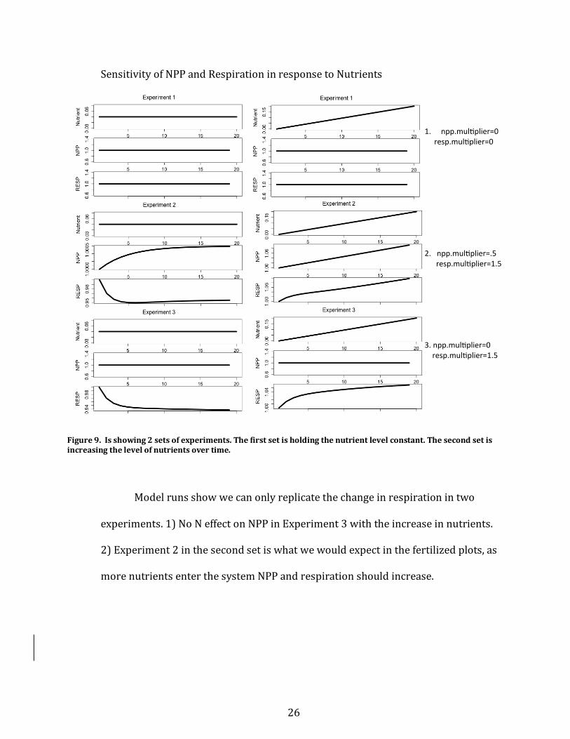
SensitivityofNPPandRespirationinresponsetoNutrients

Figure9.Isshowing2setsofexperiments.Thefirstsetisholdingthenutrientlevelconstant.Thesecondsetisincreasingthelevelofnutrientsovertime.

Modelrunsshowwecanonlyreplicatethechangeinrespirationintwo

experiments.1)NoNeffectonNPPinExperiment3withtheincreaseinnutrients.

2)Experiment2inthesecondsetiswhatwewouldexpectinthefertilizedplots,as

morenutrientsenterthesystemNPPandrespirationshouldincrease.

1.  npp.mul)plier=0resp.mul)plier=02.npp.mul)plier=.5resp.mul)plier=1.5

3.npp.mul)plier=0resp.mul)plier=1.5

27

4.Conclusions

WeconcludefromourtestingsitestheeffectsofnitrogenfertilizationinRocky

MountainNationalParksuggestslong-termnitrogenfertilizationinsignificantlydecrease

soilrespirationinfertilizedplots.Therearestudiesthatsupportourfindingsthat

fertilizationreducessoilrespiration(Kowalenkoet.al1976,Bowdenet.al2004,Olssonet.

al2005).However,theroleofnitrogendepositionmaybeabletocontrolhowfastplants

andmicrobesaredecomposingorganicmatterintheRockyMountainRegion(Bobbinket

al2010).Inthissubalpineforestecosystemmicrobialcommunitypropertiesandsoil

carbonisalteredbynitrogenfertilization.Fertilizedsoilshadlower%Cthancontrolssoils

andfertilizedsoilshadlowermicrobialbiomassCcomparedtocontrolssoils(Bootet.al

2015).Thissupportsourhypothesisthatincreaseinnitrogeninsubalpineforests

influencessoilrespiration,eventhoughitmaynotbesignificantlydifferent.Researchthat

cancontributetoourunderstandingofsoilorganicmatterturnoverratesandhowtheyare

affectedbyaddednitrogencanbeusedtoprovideinsightintothecorrelationsbetween

nitrogenfertilizationandsoilrespiration.

HasNdepositionfertilizedcontrolplots?DuetoincreasesinNdepositionor

fertilizationNdemandismet.Therewasnosignificantadditionalrespirationresponseto

fertilization.Eventhoughthecontrolplotsarenotreceivingammoniumnitratepellets,

theyarereceivingambientnitrogendeposition.Alsotemperaturewasamajorfactorinsoil

respirationrates.OurSimpleecosystemmodelwasunabletoexplainlackoffertilization

effectonsoilrespiration.Weusedasimplemodeltotesttheideathatatransient

fertilizationeffectisnowgone.Themodelresultssuggestthisisnotrealistic.Nitrogen

28

saturatedsoilsadjuststomaximumnetprimaryproduction.Controlplotsarealready

saturatedbecauseofexcessnitrogendepositionreceivedovertime.

Discussion

NitrogenFertilization

Ourfindingssuggestlongtermnitrogenfertilizationdoesnotsignificantlyaffectsoil

respirationinfertilizedandcontrolplots.Soilrespirationinboththecontrolandfertilized

plotsfollowedasimilarseasonalpattern,withthehighestratesoccurringinJulythewarm

andwetgrowingseasonandthelowestratesinOctober.Wealsofoundsignificanteffects

ofbothsoiltemperatureandmoistureonsoilrespiration,butthiswasduetoastrong

correlationbetweentemperatureandmoisture(P<0.001).Microbialactivityisaffectedby

thechangesintheavailabilityofsoilmoisture(Orchardet.al1983).Whichsupportsour

findingsthatsoilmoistureandtemperatureplaysamajorfactoronsoilrespiration.We

expectedfertilizationtoaffectcarbondynamicswithintheplotssinceoldgrowthforestare

sensitivetoincreaseinnitrogen(Hedinetal1995).In2003Sanjayet.al,foundasimilar

resultduringhismaster’sthesis:“SoilRespirationresponsestofertilization:Acomparison

oftwoforestswithdifferentnitrogendepositionhistories”.Thelackofsignificantsoil

respirationresponsefromfertilizedplotssuggestsnitrogendemandhasbeensaturatedby

chronicelevatednitrogendeposition.

29

References

AgrenG&BosattaE(1988)Nitrogensaturationofterrestrialecosystems.EnvironmentalPollution54:185–197.

Asner,G.P.,Seastedt,T.R.,&Townsend,A.R.(1997).Thedecouplingofterrestrialcarbon

andnitrogencycles.BioScience,226-234.Baron,J.S.,Rueth,H.M.,Wolfe,A.M.,Nydick,K.R.,Allstott,E.J.,Minear,J.T.,&Moraska,B.

(2000).EcosystemresponsestonitrogendepositionintheColoradoFrontRange.Ecosystems,3(4),352-368.

Baron,J.S.,DelGrosso,S.,Ojima,D.S.,Theobald,D.M.,&Parton,W.J.(2004).Nitrogen

emissionsalongtheColoradoFrontRange:responsetopopulationgrowth,landandwaterusechange,andagriculture.Ecosystemsandlandusechange(R.DeFries,G.Asner,andR.Houghton,eds.).AmericanGeophysicalUnion,Washington,DC,117-127.

Bobbink,R.,Hicks,K.,Galloway,J.,Spranger,T.,Alkemade,R.,Ashmore,M.,...&DeVries,W.

(2010).Globalassessmentofnitrogendepositioneffectsonterrestrialplantdiversity:asynthesis.Ecologicalapplications,20(1),30-59.

Boot,C.M.,Hall,E.K.,Denef,K.,&Baron,J.S.(2016).Long-termreactivenitrogenloading

alterssoilcarbonandmicrobialcommunitypropertiesinasubalpineforestecosystem.SoilBiologyandBiochemistry,92,211-220.

Bowden,R.D.,Davidson,E.,Savage,K.,Arabia,C.,&Steudler,P.(2004).Chronicnitrogen

additionsreducetotalsoilrespirationandmicrobialrespirationintemperateforestsoilsattheHarvardForest.ForestEcologyandManagement,196(1),43-56.

Bowman,W.D.,Turnbull,J.,Gleixner,G.,Neff,J.C.,Lehman,S.J.,&Townsend,A.R.(2002).

Variableeffectsofnitrogenadditionsonthestabilityandturnoverofsoilcarbon.Nature:Internationalweeklyjournalofscience,419(6910),915-917.

ChapinIII,F.S.,Matson,P.A.,&Vitousek,P.(2011).Principlesofterrestrialecosystem

ecology.SpringerScience&BusinessMedia.Fenn,M.E.,Baron,J.S.,Allen,E.B.,Rueth,H.M.,Nydick,K.R.,Geiser,L.,...&Neitlich,P.

(2003).EcologicaleffectsofnitrogendepositioninthewesternUnitedStates.BioScience,53(4),404-420.

Friedland,A.J.,Miller,E.K.,Battles,J.J.,&Thorne,J.F.(1991).Nitrogendeposition,

distributionandcyclinginasubalpinespruce-firforestintheAdirondacks,NewYork,USA.Biogeochemistry,14(1),31-55.

30

Friedlingstein,P.,Houghton,R.,Marland,G.,Hackler,J.,Boden,T.,Conway,T.,Canadell,J.,Raupach,G.,Ciais,P.,LeQuere,C.,UpdateonEmissionsCO2,NatureGeoscience3,811–8122010

Hogber,P.(2007)Nitrogenimpactsonforestcarbon.Nature.447,781-782Gruber,N.,&Galloway,J.N.(2008).AnEarth-systemperspectiveoftheglobalnitrogencycle.Nature,451(7176),293-296.Janssens,I.A.,Dieleman,W.,Luyssaert,S.,Subke,J.A.,Reichstein,M.,Ceulemans,R.,...&

Law,B.E.(2010).Reductionofforestsoilrespirationinresponsetonitrogendeposition.NatureGeoscience,3(5),315-322.

Kowalenko,C.G.,&Ivarson,K.C.(1978).Effectofmoisturecontent,temperatureand

nitrogenfertilizationoncarbondioxideevolutionfromfieldsoils.SoilBiologyandBiochemistry,10(5),417-423.

Markowski,P.,&Richardson,Y.(2011).Mesoscalemeteorologyinmidlatitudes(Vol.2).John

Wiley&Sons.Magnani,F.,Mencuccini,M.,Borghetti,M.,Berbigier,P.,Berninger,F.,Delzon,S.,...&

Kowalski,A.S.(2007).Thehumanfootprintinthecarboncycleoftemperateandborealforests.Nature,447(7146),849-851.

Nadelhoffer,K.J.,Emmett,B.A.,Gundersen,P.,Kjønaas,O.J.,Koopmans,C.J.,Schleppi,P.,...

&Wright,R.F.(1999).Nitrogendepositionmakesaminorcontributiontocarbonsequestrationintemperateforests.Nature,398(6723),145-148.

Norman,J.M.,Kucharik,C.J.,Gower,S.T.,Baldocchi,D.D.,Crill,P.M.,Rayment,M.,...&

Striegl,R.G.(1997).Acomparisonofsixmethodsformeasuringsoil-surfacecarbondioxidefluxes.JournalofGeophysicalResearch:Atmospheres(1984–2012),102(D24),28771-28777.

Orchard,V.A.,&Cook,F.J.(1983).Relationshipbetweensoilrespirationandsoilmoisture.SoilBiologyandBiochemistry,15(4),447-453.

Olsson,P.,Linder,S.,Giesler,R.,&Högberg,P.(2005).Fertilizationofborealforestreduces

bothautotrophicandheterotrophicsoilrespiration.GlobalChangeBiology,11(10),1745-1753.

Pan,Y.,Birdsey,R.A.,Fang,J.,Houghton,R.,Kauppi,P.E.,Kurz,W.A.,...&Hayes,D.(2011).

Alargeandpersistentcarbonsinkintheworld’sforests.Science,333(6045),988-993.

RDevelopmentCoreTeam(2008).R:Alanguageandenvironmentforstatistical

computing.RFoundationforStatisticalComputing,Vienna,Austria.ISBN3-900051-07-0,URLhttp://www.R-project.org.

Rueth,H.,Baron,J.,Allstott,E.,ResponsesofEngelmannspruceforeststonitrogen

31

fertilizationintheColoradoRockyMountains,EcologicalApplications13(3),pp.664-673,2003.

Ryan,M.G.(1991).Effectsofclimatechangeonplantrespiration.EcologicalApplications,1(2),157-167.

Schmidt,M.,Torn,M.,Abiven,S.,Dittmar,T.,Guggenberger,G.,Janssens,I.,

Kleber,M.,Kogel,I.,Lemann,J.,Manning,D.,Nannipieri,P.,Rasse,D.,Weiner,S.,Trumbore,S.,Persistenceofsoilorganicmatterasanecosystemproperty,Nature.Vol.478.2001.

Schlesinger,W.H.,&Andrews,J.A.(2000).Soilrespirationandtheglobalcarboncycle.

Biogeochemistry,48(1),7-20.Scott-Denton, L. E., Sparks, K. L., & Monson, R. K. (2003). Spatial and temporal controls of soil

respiration rate in a high-elevation, subalpine forest. Soil Biology and Biochemistry, 35(4), 525-534.

Vitousek,P.M.,Mooney,H.A.,Lubchenco,J.,&Melillo,J.M.(1997).Humandominationof

Earth'secosystems.Science,277(5325),494-499.Vitousek,P.M.,Aber,J.D.,Howarth,R.W.,Likens,G.E.,Matson,P.A.,Schindler,D.W.,

Schlesinger,W.H.andTilman,D.G.(1997),HUMANALTERATIONOFTHEGLOBALNITROGENCYCLE:SOURCESANDCONSEQUENCES.EcologicalApplications,7:737–750.

Waldrop,M.P.,Zak,D.R.,Sinsabaugh,R.L.,Gallo,M.,&Lauber,C.(2004).Nitrogen

depositionmodifiessoilcarbonstoragethroughchangesinmicrobialenzymaticactivity.EcologicalApplications,14(4),1172-1177.

Williams,MarkW.,andKathyA.Tonnessen."Criticalloadsforinorganicnitrogen

depositionintheColoradoFrontRange,USA."EcologicalApplications10.6(2000):1648-1665.

Wolyn,P.G.,&Mckee,T.B.(1994).Themountain-plainscirculationeastofa2-km-high

north-southbarrier.Monthlyweatherreview,122(7),1490-1508.

VantHoffJH(1898)Lecturesontheorecticalandphysicalchemisty.In:ChemicalDynamics

PartI.pp.224-229.EdwardArnold,London

32

Calculate Flux and Fit Q10 coefficient #Use soil respiration data to find the Q10 file.name <- file.choose() #read.csv("/Users/jordan/LVWS.model/Loch Vale Spreadsheet Data.csv") #data <- read.csv("/Users/jordan/LVWS.model/Loch Vale Spreadsheet Data.csv") data <- read.csv(file.name) control <- subset(data, Treatment != 'Fertilized') fert <- subset(data, Treatment == 'Fertilized') #Date = day of sample #Treatment = Control or Fertilized #Plot = location of plot #Collar = collar number #Flux = Respiration measurement #slope = #temp = temperature of soil #moisture = moisture of soil #rt = reference temperature #pressure = pressure in KPa #area = area of collar in cm^2 #depth = average collar depth #volume = volume of chamber #system = air in tubing + system #VolumeC = Volume of collar =( Collar area * Collar Depth) + chamber volume +System +Tubing #Mol of Air in System = =VolumeC/22.414/1000 #pressure = atmospheric pressure # Calculate respiration for all control data pressure <- control$pressure * 1000 #(pressure in PA) volume <- control$Volume/ 1000000 # convert cm^3/cm^3 to m^3 Ref <- control$ref # kelvin temperature correction for reference temperature of Licor R <- 8.314 #J/(K *mol) universal gas constant control.temp <- control$WST area <- control$Collar.area / 10000 # convert cm^2 to m^2 control.flux <- control$slope * pressure * volume / (R * (control.temp+273.15) * area) # Calculate respiration for all fertilized data pressure <- fert$pressure * 1000 #(pressure in PA) volume <- fert$Volume/ 1000000 # convert cm^3/cm^3 to m^3

33

Ref <- fert$ref # kelvin temperature correction for reference temperature of Licor R <- 8.314 #J/(K *mol) universal gas constant fert.temp <- fert$WST area <- fert$Collar.area / 10000 # convert cm^2 to m^2 fert.flux <- fert$slope * pressure * volume / (R * (fert.temp+273.15) * area) # Convert character dates with slashes to dates R recognizes data$Date <- as.Date(data$Date, format='%m/%d/%y') fert.obs <- data.frame(temp=fert.temp, resp=fert.flux) control.obs <- data.frame(temp=control.temp, resp=control.flux) # Fit the exponential equation to the control observations fit <- nls(resp ~ R0 * Q10 ^ ((temp-25)/10), data=control.obs, start = list(R0=10, Q10=2), trace=TRUE) control.R0 <- coef(fit)[1] control.Q10 <- coef(fit)[2] # Fit the exponential equation to the fertilized observations fit <- nls(resp ~ R0 * Q10 ^ ((temp-25)/10), data=fert.obs, start = list(R0=10, Q10=2), trace=TRUE) fert.R0 <- coef(fit)[1] fert.Q10 <- coef(fit)[2] # Before making plots, set the plot margins old.par <- par(no.readonly=TRUE) # remember the old parameters bot <- 5 left <- 5 top <- 3 right <- 1 par(mar=c(bot,left,top,right)) par(mfrow=c(1,1)) #Make plot of control data plot(control.obs$temp, control.obs$resp, main='Soil Surface Carbon Flux', pch=19, ylim=c(0,8), xlim=c(0,20), col='blue', xlab='Temperature (Celsius)', ylab='Respiration(µmol m-2 s-1)')

34

# Overlay the fertilized data as circles points(fert.obs$temp, fert.obs$resp, pch=1, col='red', ylim=c(0,8), xlim=c(0,20)) # Add the fitted curve of control data in blue to the plot min.temp <- min(control.obs$temp) max.temp <- max(control.obs$temp) control.fit.temp <- seq(min.temp, max.temp, (max.temp-min.temp)/length(control.obs$temp)) control.fit.flux <- control.R0 * control.Q10 ^ ((control.fit.temp -25)/10) lines(control.fit.temp, control.fit.flux, col='blue',lwd=5) # Add the fitted curve of fertilized data in red to the plot min.temp <- min(fert.obs$temp) max.temp <- max(fert.obs$temp) fert.fit.temp <- seq(min.temp, max.temp, (max.temp-min.temp)/length(fert.obs$temp)) fert.fit.flux <- fert.R0 * fert.Q10 ^ ((fert.fit.temp -25)/10) lines(fert.fit.temp, fert.fit.flux, col='red',lwd=5) #Add text to plots text(x=2, y=7, label="Control", col='blue') text(x=2, y=6, label="Fertilized", col='red') # Restore the old graphics parameters par(old.par)

35

Ecosystem Carbon Model Simple Land Script File land <- function(resp.multiplier=0, npp.multiplier=0){ # Parameters: longevity <- 2 # turnover time for live plants (default = 2 yr) tau.litter <- 2 # turnover time for dead plant material (default = 2 yr) tau.fast <- 20 # turnover time of fast soil organic matter (default = 20 yr) tau.slow <- 500 # turnover time of slow soil organic matter (default = 500 yr) eff.microbes <- 0.80 # efficiency of microbial respiration plant.eq <- 50 NPP.eq <- 6 # Initialize a bunch of arrays for later plotting nYears <- 20 NPP <- replicate(nYears,NA) resp.total <- replicate(nYears,NA) resp.litter <- replicate(nYears,NA) resp.fast <- replicate(nYears,NA) resp.slow <- replicate(nYears,NA) plant <- replicate(nYears,NA) litter <- replicate(nYears,NA) fast.soil <- replicate(nYears,NA) slow.soil <- replicate(nYears,NA) mortality <- replicate(nYears,0.) # Initialize mass of carbon (kg C) in plants, soil, and passive pools # These are calculated as steady-state solutions to the differential equations capacity <- plant.eq / (1-1/longevity) # resource-limited "carrying capacity" growth.rate <- NPP.eq / (plant.eq*(1-plant.eq/capacity)) death.rate <- growth.rate/longevity # fractional death per year # Initialize each pool (GtC) to be in equilibrium with NPP and decay plant[1] <- plant.eq litter[1] <- tau.litter * death.rate * plant[1] fast.soil[1] <- tau.fast/tau.litter * (1-eff.microbes) * litter[1]

36

slow.soil[1] <- tau.slow/tau.fast * (1-eff.microbes) * fast.soil[1] # Read and set up driver data for nutrients driver.data <- read.table('new.lvws.history.txt', col.names=c('year','nutrient')) nutrient <- driver.data$nutrient # Integrate the model for (i in 1:(nYears-1)){ # Adjust plant carrying capacity according to nutrients in soil current.capacity <- capacity * (1 + nutrient[i] * npp.multiplier) # If requested, enhance respiration according to nutrients too resp.enhancement <- (1 + nutrient[i] * resp.multiplier) # Apply nutrient limitation & fertilization to get updated NPP NPP[i] <- growth.rate * plant[i] * (1 - plant[i]/(current.capacity)) # Apply disturbance & mortality mortality[i] <- death.rate * plant[i] # Calculate respiration for each pool resp.litter[i] <- eff.microbes * litter[i]/tau.litter * resp.enhancement resp.fast[i] <- eff.microbes * fast.soil[i]/tau.fast * resp.enhancement resp.slow[i] <- slow.soil[i]/tau.slow * resp.enhancement resp.total[i] <- resp.litter[i] + resp.fast[i] + resp.slow[i] # Update all the carbon pools in plants and soils plant[i+1] <- plant[i] + NPP[i] - mortality[i] litter[i+1] <- litter[i] + mortality[i] - litter[i]/tau.litter * resp.enhancement fast.soil[i+1] <- fast.soil[i] + resp.enhancement * ( (1.-eff.microbes) * litter[i]/tau.litter - fast.soil[i]/tau.fast) slow.soil[i+1] <- slow.soil[i] + resp.enhancement * ( (1.-eff.microbes) * fast.soil[i]/tau.fast - slow.soil[i]/tau.slow)

37

} return(data.frame(plant=plant, litter=litter, fast.soil=fast.soil, slow.soil=slow.soil, NPP=NPP, resp.litter=resp.litter, resp.fast=resp.fast, resp.slow=resp.slow, resp.total=resp.total, nutrient=nutrient)) } # Create the 20-year history of conditions in LVWS for use in the land model nitrogen.start <- 0. nitrogen.end <- .20 step <- (nitrogen.end - nitrogen.start) / 19 nitrogen <- seq(nitrogen.start, nitrogen.end, step) #nitrogen <- replicate(20,1.05) #nitrogen[1:5] <- seq(1.01,1.05,.01) years <- 1996:2015 history <- data.frame(years=years, nitrogen=nitrogen) write.table(history, file='new.lvws.history.txt', row.names=F, col.names=F)