THERMAL NETWORK THEORY FOR SWITCHGEAR UNDER CONTINUOUS …ethesis.nitrkl.ac.in/4325/1/Thermal_Network_Theory_for_Switchgear... · THERMAL NETWORK THEORY FOR SWITCHGEAR UNDER CONTINUOUS

THERMAL NETWORK THEORY FOR SWITCHGEAR UNDER CONTINUOUS CURRENT

A THESIS SUBMITTED IN PARTIAL FULFILLMENT

OF THE REQUIREMENTS FOR THE DEGREE OF

Master of Technology In

Machine Design and Analysis

By

KRISHNA SWAMY CHERUKURI

Department of Mechanical Engineering

National Institute of Technology

Rourkela

2007

THERMAL NETWORK THEORY FOR SWITCHGEAR UNDER CONTINUOUS CURRENT

A THESIS SUBMITTED IN PARTIAL FULFILLMENT

OF THE REQUIREMENTS FOR THE DEGREE OF

Master of Technology In

Mechanical Engineering

By

KRISHNA SWAMY CHERUKURI

Under the Guidance of

Dr. DAYAL R. PARHI

Department of Mechanical Engineering

National Institute of Technology

Rourkela

2007

National Institute of Technology Rourkela

CERTIFICATE

This is to certify the thesis entitled, “Thermal Network Theory for Switchgear under Continuous

Current” submitted by Sri Krishna Swamy Cherukuri in partial fulfillment of the requirements

for the award of Master of Technology in Mechanical Engineering with specialization in

“Machine Design and Analysis” at the National Institute of Technology, Rourkela is an authentic

work carried out by him under my supervision and guidance.

To the best of my knowledge, the matter embodied in the thesis has not been submitted to any

other University / Institute for the award of any Degree or Diploma.

Date Dr. Dayal R. Parhi

Dept. of Mechanical Engg. National Institute of Technology

Rourkela – 769008

ACKNOWLEDGEMENT

Successful completion of work will never be one man’s task. It requires hard work in right

direction. There are many who have helped to make my experience as a student a rewarding

one.

In particular, I express my gratitude and deep regards to my thesis guide Dr. Dayal R. Parhi

first for his valuable guidance, constant encouragement & kind co-operation throughout

period of work which has been instrumental in the success of thesis.

I also express my gratitude & regards to Deepak Raorane (COE, GE, IIC, Hyderabad),

company guide Debabrata Mukherjee and Sudhakar Pachunoori for their scientific advice

and eagerness to help during my work at GE, IIC, Hyderabad

I also express my sincere gratitude to Dr. B. K. Nanda, Head of the Department, Mechanical

Engineering, for providing valuable departmental facilities.

I would like to thank Prof. N. Kavi, P.G Coordinator, Mechanical Engineering Department

and Prof. K.R.Patel, Faculty Adviser.

I thank my friend, Jaydev Sirimamilla who helped me and turned the task of learning

software required for the project a joy.

I would like to thank my fellow post-graduate students, Tulasi Ram, SadikaBaba, Rajesh and

Sundeep who made learning science a joy.

Krishna Swamy Cherukuri

i

TABLE OF CONTENTS CHAPTER Page No

Acknowledgement i

Abstract v

List of Figures vi

List of Tables viii

1. INTRODUCTION 1-2

1.1 Background 1

1.2 Objective 1

2. LITERATURE SURVEY 3-6

2.1 Thermal Network Theory 3

2.2 Contact resistance 3

2.2.1 Electrical Contact Resistance 4

2.2.2 Thermal Contact Resistance 5

3. INTRODUCTION TO SWITCH GEAR 7-13

3.1 Introduction 7

3.2 Switch Gear 7

3.3 Circuit Breaker 9

3.4 Current Flow Path in a Switch Gear 11

4. THERMAL NETWORK THEORY 14-35

4.1 Introduction 14

4.2 Electrical and Thermal Analogy 15


4.4 The Lumped-parameter Method for Steady State Solution 17

4.5 The Lumped-Parameter Method for Transient Solution 18

4.6 Building Thermal Network 18

4.7 Nodes 19

4.8 Conductors 20

4.9 Criteria for Selecting Nodes 21

4.10 Node Equations 22

ii

4.11 Node Equation at Joint 28

4.12 Convection 32

4.12.1 Convective Heat Transfer Co-efficient 32

4.12(a) h Correlations for Vertical Plate in Natural Convection 33

4.12(b) h Correlations for Horizontal Plate in Natural Convection 34

4.1.3 Effect of Radiation 35

5. JOINT RESISTANCE 36-47

5.1 Types of Joints 36

5.2 Types of Electrical Contacts 37

5.3 Electrical Contact Resistance 39

5.4 Calculation of Electrical Contact Resistance 40

5.2.1 Maxwell’s Formula 40

5.2.2 Greenwood’s Formula 40

5.2.3 Empirical Relations 41

5.5 Thermal Contact Resistance 43

5.5.1 Relation Based on Thermo-Electromechanical Properties 47

6. PROBLEM SOLVING PREOCESS 48-67

6.1 Problem Definition 48

6.2 Steps in Solving the Problem 48

6.2.1 Electrical Network Diagram 49

6.2.2 Electrical Resistance Calculation 53

6.2.3 Comparison with Measured Value 54

6.2.4 Thermal Network Diagram 54

6.2.5 Calculation of Input Parameters 59

6.2.6 Convective Heat Transfer Co-efficient Calculation 59

6.3 Analytical Tool to Calculate Temperatures 59

6.3.1 Input Sheet 60

6.3.2 Joints sheet 62

6.3.3 Nodes Sheet 64

6.3.4 Network Sheet 66

6.3.5 Output Sheet 67

iii

7. RESULTS 68-80

7.1 Frame 3 68

7.1.1 Reasons for Temperature Deviation 69

7.1.2 Regions of Maximum Deviation 70

7.1.3 Results Comparison 70

7.1.3(a) Phase A 70

7.1.3(b) Phase B 72

7.1.3(c) Phase C 74

7.1.4 Temperature Prediction 75

7.1.4(a) Change in Run –In Geometry 75

7.1.4(b) Change in Heat Sink Surface Area 76

7.1.4(c) Increasing Cluster Contact Force 78

7.2 FRAME 1 79

8. CONCLUSION AND FURTHER WORK 81-82

8.1 Contribution 81

8.2 Conclusion 81

8.3 Further Work 82

9. REFERENCES 83-85

APPENDIX-A

Visual Basic Code used in Analytical Tool 86-98

iv

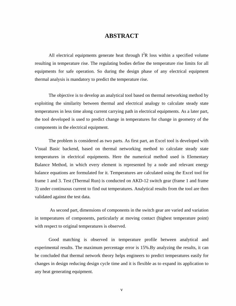
ABSTRACT

All electrical equipments generate heat through I2R loss within a specified volume

resulting in temperature rise. The regulating bodies define the temperature rise limits for all

equipments for safe operation. So during the design phase of any electrical equipment

thermal analysis is mandatory to predict the temperature rise.

The objective is to develop an analytical tool based on thermal networking method by

exploiting the similarity between thermal and electrical analogy to calculate steady state

temperatures in less time along current carrying path in electrical equipments. As a later part,

the tool developed is used to predict change in temperatures for change in geometry of the

components in the electrical equipment.

The problem is considered as two parts. As first part, an Excel tool is developed with

Visual Basic backend, based on thermal networking method to calculate steady state

temperatures in electrical equipments. Here the numerical method used is Elementary

Balance Method, in which every element is represented by a node and relevant energy

balance equations are formulated for it. Temperatures are calculated using the Excel tool for

frame 1 and 3. Test (Thermal Run) is conducted on AKD-12 switch gear (frame 1 and frame

3) under continuous current to find out temperatures. Analytical results from the tool are then

validated against the test data.

As second part, dimensions of components in the switch gear are varied and variation

in temperatures of components, particularly at moving contact (highest temperature point)

with respect to original temperatures is observed.

Good matching is observed in temperature profile between analytical and

experimental results. The maximum percentage error is 15%.By analyzing the results, it can

be concluded that thermal network theory helps engineers to predict temperatures easily for

changes in design reducing design cycle time and it is flexible as to expand its application to

any heat generating equipment.

v

LIST OF FIGURES

Page No

Figure 3.1 GE Switch Gears Figure 8

Figure 3.2 MCB 10

Figure 3.3 Powervac MV Vacuum Distribution Breaker 10

Figure 3.4 115,000 V Breaker at Generating Station 10

Figure 3.5 1250 A air circuit Breaker 10

Figure 3.6 Switch Gear Line Diagram 11

Figure 3.7 Switch Gear Line Diagram showing Joints 12

Figure 4.1 Network Representation 23

Figure 4.2 Heat Balance at a Node 23

Figure 4.3 Energy Balance at Node 2 26

Figure 4.4 Network Representation at a joint 28

Figure 5.1 Effect of Contact Pressure on Contact Resistance 40

Figure 5.2 Set of Circular Contact Spots showing the Symbol Notation 41

Figure 5.3 – Constriction of Heat Flow through an Interface formed by two Materials. 43

Figure 5.4 Temperature drop on either side of interface 44

Figure 5.5 Heat transfer paths at an interface 45

Figure 5.6 Thermal Resistance Network for nonconforming rough contacts 45

Figure 5.7 Thermal contact problem. 46

Figure 6.1 Electrical Network diagram for frame 1 50


Figure 6.3 Electrical Network Diagram for frame 3 with3 phases 52

Figure 6.4 Thermal Network Diagram for frame 1 55


Figure 6.6 Thermal Network Diagram for Cluster Pad region 57

Figure 6.7 Input Sheet 61

Figure 6.8 Input Form for Joints 62

Figure 6.9 Joints Sheet 63

vi

Figure 6.10 Input Form for Nodes 64

Figure 6.11 Nodes Sheet 65

Figure 6.12 Network Sheet 66

Figure 6.13 Output Sheet 67

Figure 7.1 Frame 3 Temperature profile 68

Figure 7.2 Temperatures comparison for Phase A 72

Figure 7.3 Temperatures comparison without Proximity Effect 72

Figure 7.4 Temperatures comparison for Phase B 73


Figure 7.6 Temperatures comparison for Phase C 74


Figure 7.8 Temperature Profile with change in Run-in Geometry 76

Figure7.9 Temperature variation by doubling Surface Area 77

Figure7.10 Temperature variation for change in Cluster Contact Force 78

Figure7.11 Frame -1 Temperature Profile 80

vii

LIST OF TABLES

Page No

Table 3.1 Electrical and Thermal Analogy 15

Table 5.1 K Factor Values 43

Table 5.2 – Thermal Contact Conductance Models 46

Table 7.1 Temperatures at Different Point in Frame3 69

Table 7.2 Temperatures on Phase A 71

Table 7.3 Run-In Geometry 75

Table 7.4Analytical Temperatures with and without change in Run-In Dimensions 75

Table 7.5 Analytical Temperatures Comparison by doubling the Heat Sink Surface Area 77

Table 7.6 Analytical Temperatures Comparison by increasing Contact Force at clusters 78

Table 7.7 Temperatures for Frame1 79

viii

1. INTRODUCTION

This chapter gives an overview of the project work reported in the thesis. First,

background of the project work is outlined followed by the objective and methodology

followed to achieve the objective.

1.1 BACKGROUND



equipments for safe operation. So during the design phase of any thermal equipment thermal

analysis is mandatory to predict the temperature rise. Bypassing thermal analysis precludes

design optimization.

Thermal analysis is done either by building a laboratory model or by simulation using

simulation softwares. Generally once the basic design is completed, laboratory model is built

to observe the response of the system. Later certain changes are incorporated to arrive at

optimum design. Rebuilding the model for every change incorporated becomes a costly affair.

So simulation work is carried out at this stage using simulation software to predict the

response of the system for the changes made.

By this, though cost involved in rebuilding the lab model is cut down, time required

in predicting the response of the system for new design or changes cannot be avoided. This is

so because, in simulation software rebuilding the model, meshing, changing the boundary

conditions and running the solution for any change in geometry of the components involves

considerable time. So, one is interested to predict temperature variations in very less time

using simple mathematical calculations even at the sacrifice of accuracy to certain extent.

1.2 OBJECTIVE




1



Following methodology is followed to achieve the objective. The problem is

considered as two parts. As first part, an Excel tool is developed with Visual Basic backend,

based on thermal networking method to calculate steady state temperatures in electrical

equipments. Here the numerical method used is Elementary Balance Method, in which every

element is represented by a node and relevant energy balance equations are formulated for it.

Analytical calculations are carried out and temperatures are calculated using the Excel tool

for frame 1 and 3. Test (Thermal Run) is conducted on AKD-12 switchgear, frame 1 and

frame 3 under continuous current to find out temperatures at different points along the

current flow path. Analytical results from the tool are then validated against the test data.

Good matching is observed in temperature profile between analytical and experimental

results.




2

2. LITERATURE SURVEY

This chapter surveys the literature in the areas of thermal network modeling, electrical

contact resistance and thermal contact resistance.

2.1THERMAL NETWORK THEORY

Peter and Hans [1] have carried out thermal simulation of a circuit Breaker to find out steady

state temperatures considering all modes of heat transfer. The analysis is done based on

software developed using thermal networking with a capacity of 32000 nodes. The paper

explains the thermo- Electrical coupling to represent electrical carrying conductor by thermal

components.

Correspondence from IEEE [2] describes a relatively simple method for manual thermal

computations, particularly useful for electronic equipment where all types of heat transfer

must be taken into account. The method involves construction of a simplified thermal

network diagram for the equipment. The method of thermal computation described here

exploits the similarity between thermal and electrical analogy, shown in table [4.1].

Hiroshi and Kazunori [3] have described the way to develop thermal network diagram for

low voltage circuit breaker.

Hefner and Blackburn published a paper [9] giving thermal Component simulation for

electro-thermal network simulation. It explains the structure of the electro-thermal

semiconductor device models indicating the interaction with the thermal and electrical

networks through the electrical and thermal terminals, respectively.

2.2 CONTACT RESISTANCE

An accurate knowledge of contact mechanics, that is, the pressure distribution, the size of

contact area, and the mean separation between surface planes as functions of applied load,

and the geometrical and mechanical characteristics/properties of the contacting bodies, plays

an important role in predicting and analyzing thermal and electrical contact resistance and

many tribological phenomena.[6]

3

2.2.1 Electrical Contact Resistance

The calculation of the contact resistance between two rough electrodes is a difficult task,

since the contact interface comprises many spots corresponding to more or less conducting

paths for the electrons [4].

In 1966, J. A. Greenwood published a paper entitled [12] in which the author derived a

formula [5.2] for the constriction resistance of a set of circular spots [Fig.5.2], with each spot

located at the end of a metallic electrode. The electrodes communicate via the spots with no

interface film between them. In the same paper author presented a formula resulting from an

approximation which holds when there is no correlation between the size of a given spot and

its position.

For some ten years now, contact resistance has been computed numerically mainly by

Nakamura and Minowa [13], who use the finite element method (FEM) and the boundary

element method (BEM) from a different point of view, considering a system of two cubic

electrodes communicating through square spots.

Finally, it should also be mentioned that a recent paper by R. S. Timsit reviews the

dependence of electrical resistance on the shape and dimensions of the contact spots [14].

Maxwell’s formulation for single contact spot is given by formula [5.1]. With increase in

contact pressure, the electrical contact resistance decreases at the joint as shown in graph

[4.1].

In the paper published by Peter and Hans [1], electrical contact resistance is given in terms of

contact force, contact material type and shape of the contact, shown by formula [5.3]. Based

on these formulae, empirical relations [5.4, 5.5] are developed which can be used for bolted

and spring loaded contacts for different materials. Those empirical relations are used here to

calculate the electrical contact resistance.

4

2.2.2 Thermal Contact Resistance

Heat transfer across interfaces formed by mechanical contact of nonconforming rough solids

occurs in a wide range of applications, such as microelectronics cooling, spacecraft structures,

satellite bolted joints, nuclear engineering, ball bearings, and heat exchangers. Because of

roughness of the contacting surfaces, real contacts in the form of micro contacts occur only at

the top of surface asperities, which are a small portion of the nominal contact area, normally

less than a few percent. As a result of curvature or out-of flatness of the contacting bodies, a

macro contact area is formed, the area where the micro contacts are distributed.

Two sets of resistances in series can be used to represent the thermal contact resistance (TCR)

for a joint, the large scale or macroscopic constriction resistance RL and the small-scale or

microscopic constriction resistance Rs as shown in formula [5.7].

Cooper et al. [15] studied the contact conductance of rough, conforming metals experiencing

light to moderate pressure. The model presumes that the micro contacts deform plastically.

Mikic [16] developed models for the macroscopic and microscopic contact conductance that

took into account non-uniform pressure distributions, but did not specify how the

distributions were determined. The microscopic conductance model uses the plastic

deformation model of Cooper, et al. (1969).

Thomas and Sayles [17] studied the relative effects of waviness and roughness on thermal

contact conductance. They observe that the total roughness of a specimen is related to its size,

defining a dimensionless waviness number.

Yovanovich [18] refined the model of Cooper, et al. (1969) for plastic deformation of

microscopic contacts on conforming surfaces.

Lambert [19] and Lambert and Fletcher [20] developed a model for the thermal contact

conductance of spherical rough metals that is valid in regions removed from the limiting

cases of rough/flat, smooth/spherical surfaces. It is, however, a single macro contact model,

and requires loading on the macrocontact as well as the surface geometry of the contact. In

5

multiple macrocontact situations, such as those encountered in large area contacts, it is

difficult to estimate number of macrocontact, much less the loading on each macrocontact.

Table 5.1 lists the dimensional and non-dimensional contact conductance correlations

reviewed in this section.

Peter and Hans published a paper in which the thermal contact resistances are deduced from

the electrical contact resistances. [1] The formulae used [5.8] here for thermal contact

resistance calculations are based on this paper. The thermal conductivity of the contacts is

increased by a factor of 2.1 to account for the thermal conductivity of the air in the voids of

the contact area.

6

3. INTRODUCTION TO SWITCHGEAR

3.1 INTRODUCTION

Circuit protection devices are needed to protect personnel and circuits from hazardous

conditions. The hazardous conditions can be caused by a direct short, excessive current or

excessive heat. Circuit protection devices are always connected in series with the circuit

being protected.

Every one is familiar with low voltage switches and rewire-able fuses. A switch is

used for opening and closing an electric circuit and a fuse is used for over current protection.

Every electric circuit needs a switching device (Switch) and a protective device (Fuse). The

switching and protective devices have been developed in various forms depending voltage

and current. Switchgear is a general term covering a wide range of equipment concerned with

switching and protection.

3.2 SWITCHGEAR

The term switchgear, commonly used in association with the electric power system,

or grid, refers to the combination of electrical disconnects and/or circuit breakers used to

isolate electrical equipment. All equipments associated with the fault clearing process are

covered by the term “Switchgear”. Switchgear is an essential part of power system and also

that of any electric circuit. Between the generating station and final load point, there are

several voltage levels and fault levels. Hence, in various applications, the requirements of

switchgear vary depending upon the location, ratings and switching duty. Switchgear

includes switches, fuses, circuit breakers, isolators, relays, control panels, lightening arresters,

current transformers and various associated equipments.

3.2.1Protective Relay: The protective relays are the automatic devices, which can sense the

fault and send instructions to the associated circuit breaker to open.

3.2.2Circuit Breakers: Circuit breakers are the switching and current interrupting devices.

Basically a circuit breaker comprises a set of fixed and movable contacts. The contacts can

be separated by means of an operating mechanism. The separation of the current carrying

7

contacts produces an arc. The arc is extinguished by a suitable medium like dielectric oil, air,

vacuum and SF6 gas.

3.2.3 Isolators: Isolators are disconnecting switches, which can be used for disconnecting a

circuit under no current condition. They are generally installed along with circuit breaker. An

isolator can be opened after the circuit breaker. After opening the isolator the earthing switch

can be closed to discharge the charges to the ground.

3.2.4 Transformers: The current transformers and the potential transformers are used for

transforming the current and voltage to a lower value for the purpose of measurement,

protection and control.

3.2.5 Lightening Arresters: Lightening arresters (surge arresters) divert the over-voltages

to earth and protect the sub-station equipment from over voltages.

Some of GE Switchgear products:

Figure 3.1 GE Switchgears A - AKD 10 Low Voltage Metal Enclosed

B - Paralleling switch Gear

C - Entellisys Low Voltage switch Gear

D - Power/Vac® Medium Voltage Metal Clad Switch Gear

8

3.3 CIRCUIT BREAKER

A circuit breaker is an automatically-operated electrical switch designed to protect an

electrical circuit from damage caused by overload or short circuit. It is a device to open or

close an electric power circuit either during normal power system operation or during

abnormal conditions. During abnormal conditions, when excessive current develops, a circuit

breaker opens to protect equipment and surroundings from possible damage due to excess

current. These abnormal currents are usually the result of short circuits created by lightning,

accidents, deterioration of equipment, or sustained overloads. Unlike a fuse, which operates

once and then has to be replaced, a circuit breaker can be reset (either manually or

automatically) to resume normal operation. Circuit breakers are made in varying sizes, from

small devices that protect an individual household appliance up to large switchgear designed

to protect high voltage circuits feeding an entire city. Based on voltage, switch gears are

classified as

3.3.1 Low voltage Circuit Breakers

Low voltage circuit breakers have voltage ratings from 250 to 600 V AC and 250 to 700 V

DC. They are two types.

MCB-(Miniature Circuit Breaker Rated current is not more than 100 A.

MCCB-(Molded Case Circuit Breaker) Rated current is up to 1000 A.

Figure 3.2 MCB Figure 3.3 PowerVac - MV Vacuum Distribution Breaker

rated up to 72.5 kV

3.3.2 Medium Voltage Breakers

Medium voltage circuit breakers are

9

3.3.3 High-Voltage Breakers

nely available up to 765 kV AC. They are broadly classified

3. Air blast

High voltage breakers are routi

by the medium used to extinguish the arc as:

1. Oil-filled (dead tank and live tank)

2. Oil-filled (minimum oil volume) 4. Sulfur hexafluoride

Figure 3.4 1200 A, 3-pole 115,000 V Figure 3.5 Front panel of a 1250 A air

Small circuit breakers are either installed directly in equipment, or are arranged in a

breaker

3.4 CURRENT FLOW PATH IN SWITCHGEAR

Current flow path in switchgear involves many components of different cross sections

joined

Breaker at a generating station circuit breaker manufactured by ABB

panel. Power circuit breakers are built into switchgear cabinets. High-voltage

breakers may be free-standing outdoor equipment or a component of a gas-insulated

switchgear line-up

with different types of joints and contacts. Generally joints involved are bolted joints

and spring contacts. The components in the current flow path are test links, power connects,

lower vertical busbars, run-ins, cluster fingers, cluster pad, line terminal, flexible conductors,

moving conductors, load terminal, runbacks, upper vertical busbars and outgoing horizontal

busbars. Figure 3.6 shows line diagram of current flow path for switchgear. Current enters

the switchgear through test link which is connected to power source. Current then flows to

10

http://www.answers.com/topic/circuit-breaker-115-kv-jpg

http://www.answers.com/topic/largecircuitbreaker-jpg

lower vertical busbar thorough power connect. Power connect is a clamp like device used for

joining horizontal test links to vertical busbars.

Figure3.6 Switchgear Line Diagram

A busbar in electrical power distribution refers to thick strips of copper or aluminum

that conduct electricity within a switchboard, distribution board, substation or other electrical

apparatus. From busbar, current flow to circuit breaker through run-in, cluster fingers and

cluster pad. Run-ins are horizontal strips that connect gear with circuit breaker electrically.

Cluster fingers are spring loaded thin strips connecting run-ins with cluster pad. Components

in a circuit breaker are line terminal, flexible conductors, moving conductors and load

terminal. Current from circuit breaker flows through runbacks to upper vertical busbars.

From vertical busbars, current leaves the switch gear through power connect and horizontal

busbars.

11

Figure3.7 Switchgear line Diagram Showing Joints

Figure 3.7 shows joints between different components in the switchgear. Joints at

cluster fingers and moving contact are spring loaded contacts. All the remaining joints are

bolted joints with bolts of different sizes and numbers depending upon the clamping force

required at the joint. Except the test links and horizontal busbars, all the components are

placed inside a compartment as shown by dotted line. Compartment with busbars is called

busbar compartment and compartment with circuit breaker is called breaker compartment.

12

4. THERMAL NETWORK THEORY

4.1 INTRODUCTION

During the design of electrical and electronic equipments, thermal analysis of the

system is very essential and disregard of a thermal analysis may lead to inadequate thermal

design. Sometimes schedules and cost aspects exclude construction of thermal laboratory

models which many a times lands up in severe financial penalties. In some instances such

analysis is bypassed because of its complexity. This bypassing precludes design optimization.

Thermal deficiencies in performance of the equipment may then result.

So conducting thermal analysis for any electrical system is inevitable either by

building a laboratory model or by simulating the thermal analysis using simulation software.

Generally once the basic design is completed, laboratory model is built to observe the

response of the system. Later certain changes are incorporated to arrive at optimum design.

Rebuilding the model for every change incorporated becomes a costly affair. So simulation

work is carried out at this stage using simulation software to predict the response of the

system for the changes made.

Thermal simulation can be carried out using many types of software like ANSYS,

CFD, FLUX etc and results can be predicted very precisely. By this, though cost involved in

rebuilding the lab model is cut down, time required in predicting the response of the system

for new design or changes cannot be avoided. This is so because, in simulation software

rebuilding the model, meshing, changing the boundary conditions and running the solution

for any change in geometry of the components involves considerable time. So one is

interested to have an analytical tool which can predict the results in lesser time even by

compromising with the accuracy of results up to some extent. This gave birth to a relatively

simple method for manual thermal computations, particularly useful for electronic and

electrical equipment where all types of heat transfer must be taken into account. The method

involves construction of a simplified thermal network diagram for the equipment, developing

energy equation at each node and solving for temperature rise. When good judgment is used,

predicted temperature values approach actual ones.

13

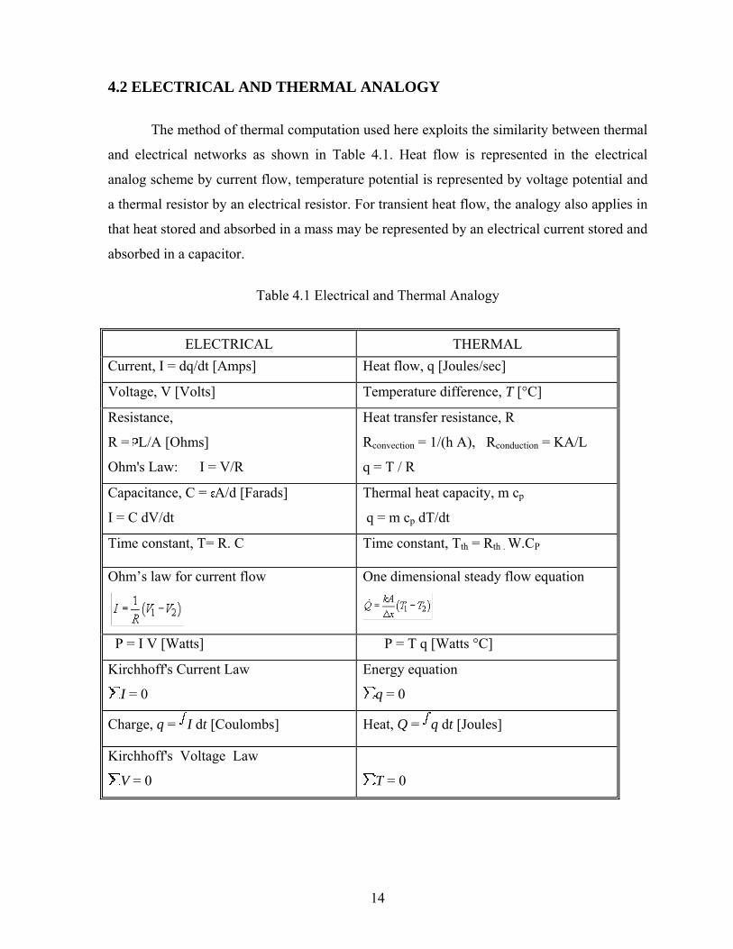
4.2 ELECTRICAL AND THERMAL ANALOGY

The method of thermal computation used here exploits the similarity between thermal

and electrical networks as shown in Table 4.1. Heat flow is represented in the electrical

analog scheme by current flow, temperature potential is represented by voltage potential and

a thermal resistor by an electrical resistor. For transient heat flow, the analogy also applies in

that heat stored and absorbed in a mass may be represented by an electrical current stored and

absorbed in a capacitor.

Table 4.1 Electrical and Thermal Analogy

ELECTRICAL THERMAL Current, I = dq/dt [Amps] Heat flow, q [Joules/sec]

Voltage, V [Volts] Temperature difference, T [°C]

Resistance,

R = L/A [Ohms]

Ohm's Law: I = V/R

Heat transfer resistance, R

Rconvection = 1/(h A), Rconduction = KA/L

q = T / R

Capacitance, C = A/d [Farads]

I = C dV/dt

Thermal heat capacity, m cp

q = m cp dT/dt

Time constant, T= R. C Time constant, Tth = Rth . W.CP

Ohm’s law for current flow

One dimensional steady flow equation

P = I V [Watts] P = T q [Watts °C]

Kirchhoff's Current Law

I = 0

Energy equation

q = 0

Charge, q = I dt [Coulombs] Heat, Q = q dt [Joules]

Kirchhoff's Voltage Law

V = 0

T = 0

14

Current flow through resistor, stored in

capacitor

Heat flow to ambient ,stored in mass of

material of specific heat cp

One dimensional current flow trough RC

network

One dimensional transient heat flow

through bar

4.3 THERMAL NETWORK THEORY

The finite difference method provides the basis for converting a distributed parameter

description of a system into a lumped parameter model of that system. We can expand the

concept of a finite node to include a larger macroscopic control volume (which physically

may be very large or small). In connecting individual control volumes, it is often useful to

use an electrical analogy to describe the system. In thermal systems, this electrical analogy

gives rise to the so-called thermal network model.

A thermal network is a representation (model) of the thermal characteristics of any

system modeled by considering points (nodes) at discrete parts of the system that are linked

by conductors through which heat may flow. This type of thermal network is often described

as a lumped parameter model because the thermal properties, such as the heat capacity, of a

part of the system are “lumped” together on the node representing that part.

The method developed here is called the Equivalent Thermal Network and takes

advantage of the theory of analogy between electrical and thermal elements. In steady state

temperature rise computations, current generators are used to represent heat generators, and

electrical resistances to represent the internal thermal conduction resistances. In transient heat

15

flow condition, capacitor is connected in parallel to represent the heat stored in the body

along with heat generator and thermal resistance. Here the mathematical model is based on a

numerical method called Elementary Balance Method, in which every element is represented

by a node and relevant energy balance equations are formulated for it.

4.4 THE LUMPED-PARAMETER METHOD FOR STEADY STATE SOLUTION

The lumped-parameter method involves dividing the object being analyzed into a

network of discrete nodes connected by thermal conductors. Each node is considered to be

isothermal i.e. has a single temperature associated with it.

To determine the steady state a heat balance is applied to each node,

Q 0=∑ (4.1)

Where Q represents heat input, and the removal of heat is regarded as a negative Q. The

symbol signifies a summation. In words, this can be stated: ∑

At any node, HEAT IN = HEAT OUT

Equation 4.1 is applied to each node in the model to obtain a system of simultaneous

equations from which all nodal temperatures are calculated.

4.5 THE LUMPED-PARAMETER METHOD FOR TRANSIENT SOLUTION

For evolution of temperatures in a model during the transient stage (not just the final

steady-state values) then the node equation acquires a time-derivative on the right-hand side.

The energy equation is written as dTQ m.cdt

=∑ (4.2)

Where, m is the mass of the node and C the specific heat capacity.

The derivative is approximated by finite differences (dT/dt).

Applying the above equation to all nodes, gives a system of algebraic equations that are

solved for temperature T at time t+dt. The solution is done by iterative method.

As the highest temperatures occur after the transient phase is over and the steady state

(thermal equilibrium) has been reached, we are interested to calculate the steady state

temperatures and so the entire work is concentrated on one dimensional steady state solution

16

by lumped parameter method. Most of the thermal calculations for electrical equipments are

limited to one dimensional only.

4.6 BUILDING THERMAL NETWORK

Building thermal network diagram for electrical equipment involves visualizing it as

thermal network with thermal resistances, heat generators and thermal capacitors. As the

work is limited to steady state, thermal capacitors are absent. First the entire structure is

descritized into number of nodes, each node representing a component with certain mass i.e.

a lumped mass. The nodes are taken as three types- diffusion nodes, boundary nodes and

arithmetic nodes. Each node is connected to the other by a conductor which represents

internal conduction resistance or convection resistance or radiation resistance. Conductors

are considered as two types—linear conductor and radiation conductors. Due to the current

flow in a element (node), there is some internal heat generation due to I2R loss and that

amount of heat is added as heat input at the corresponding node. With this the equipment is

represented as a network with different types of nodes with heat generation and connected by

different types of conductors.

4.7 NODES

At nodes energy is conserved. Each node has a single characteristic temperature ‘T’.

Nodes may represent the temperature of a finite volume of material. There are three types of

nodes, classified by their capacitance or ability to transiently store or release thermal energy.

4.7.1 Diffusion Nodes: Diffusion nodes have a finite capacitance ‘C’, usually equal to the

product of mass and specific heat (mCp or ρVCp). Diffusion nodes may represent a finite

volume and mass. These nodes are used in transient analysis.

4.7.2 Arithmetic Nodes: rithmetic nodes have zero capacitance. Energy flowing into an

arithmetic node must balance the energy flowing out at all times. These nodes are used in

steady state analysis as no heat is accumulated in the body once the system comes to

thermal equilibrium and all the heat in is equal to heat out. Heat source is added to these

nodes.

17

4.7.3 Boundary Nodes: Boundary nodes have an infinite capacitance, and hence usually

represent sources or sinks, large masses, or ideally controlled temperature zones. Air is

represented using these nodes.

4.8 CONDUCTORS

Conductors describe the means by which heat flows from one node to another. Each

conductor has a single characteristic conductance “G” (inverse of resistance). Conductors

represent energy paths via solid conduction, contact conduction, convection, advection,

radiation, etc. There are two types of conductors.

4.8.1 Linear Conductors: Linear conductors transport heat in direct proportion to the

difference in nodal temperatures

(4.3) 1 2 1 2Q G(T T− = − )

Q1-2 is the heat flow from node 1 to node 2 through a conductor of conductance G

T1 is the temperature of node 1


Usually, linear conductors represent solid conduction with ‘G’, calculated as the product of

the material conductivity and inter nodal cross-sectional area, divided by the distance

between node centers.

KAGL

= (4.4)

Linear conductors may also represent convection conductance with ‘G’, calculated as the

product of convective heat transfer coefficient ‘h’ and surface area ‘a’. Here we represent

convective conductance by H to avoid confusion.

(4.5) H = h*a

4.8.2 Radiation Conductors: Radiation conductors transport heat according to the

difference in the fourth power of absolute temperature.

(4.6) 4 41 2 1 2Q G(T T− = − )

They are used almost exclusively for radiation heat transfer, with

18

1 1 2 1G F− A= σε (4.7)

σ is the Stefan-Bolt Mann constant

ε1 is the emissivity of node 1

A1 is the area of node 1 and

F1-2 is the form factor from node 1 to node 2

4.9 CRITERIA FOR SELECTING NODES

Generally any equipment contains many components connected by joints. The entire

equipment can be divided into number of nodes, with a new node wherever

1. There is change in cross section or shape of the component.

2. Joint occurs. New node is considered to represent the joint between the two elements.

3. Length of the component is large. The same component is considered as more than

one node and the number of nodes to be considered depends on the accuracy required.

More nodes are considered for better temperature distribution. But one has to strike a

balance between the increased complexity of the network and the required accuracy.

4. Imaginary or dummy nodes are introduced wherever branching or joining of

resistances occurs to generalize the node equations. No thermal properties are

considered for dummy nodes.

4.10 NODE EQUATIONS

As the general phenomenon, when current flows through a conductor, heat is

generated in the conductor due to I2R loss and temperature of the conductor rises above the

ambient air temperature. Heat is transferred from one end of the conductor to the other by

thermal conduction and at the same time heat is lost to atmospheric air by convection

bringing the system to thermal stability after certain time period. (Neglecting radiation) The

same is explained schematically as follows. Consider a stepped bar with rectangular cross

section as shown in fig 4.1(1). Current “I” flows form the left hand side and the bar is placed

in ambient air. The bar is descritized into parts for change in cross section giving 3 parts.

Each part is lumped and considered as a small node. Node represents the part in mass and

thermal characteristics. The internal thermal conduction resistance of a part is represented by

a resistance symbol (Rc).

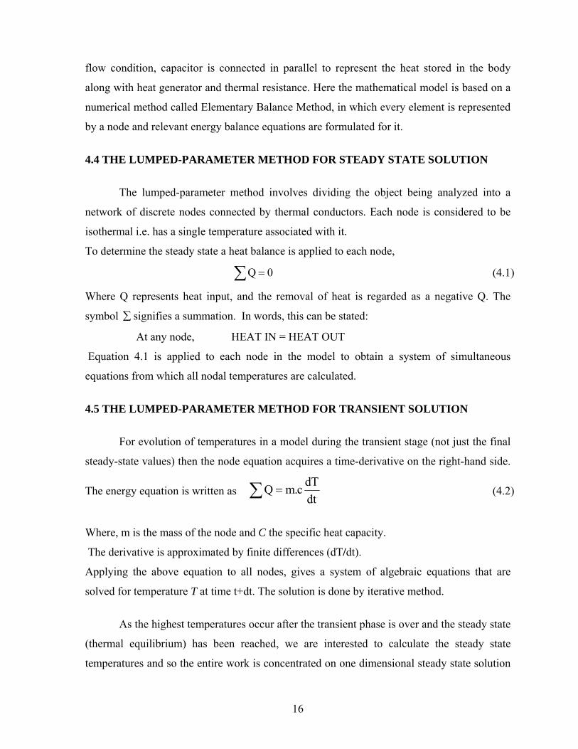
19

Figure 4.1 Network Diagram

Resistance (Rc1) represents the thermal conduction resistance between node1 and

node 2. It is equal to sum of fifty percent of conduction resistance of part one and fifty

percent of conduction resistance of part two. Assembling the nodes, thermal resistances and

heat generators, thermal network diagram is developed as shown in figure 4.1(6). There are 3

nodes-- node1, node2 and node3 connected by thermal conduction resistances Rc1, Rc2, Rc3.

Each node is connected to the ambient air by convection resistance Rth—convection

20

resistances Rth1, Rth2, Rth3.The heat generated (Q) by I2R loss in each part is represented by

Q1, Q2 and Q3 and added as heat inputs at corresponding nodes

The next step is to develop energy balance equation at each node. The elementary energy

balance equation (steady state) is given as

Figure 4.2 Energy Balance at a Node

I.e. the heat input to a node by different modes is equal to heat lost from the node by different

modes. It can be written as

For a node I, the nodal equation can be written mathematically as:

i ambienti 1 i i i 1

iC(i 1) Ci th (i)

(T T )(T T ) (T T )QR R R− +

−

−− −+ = + (4.8)

4.10.1 Internal Heat Generation

Internal heat generated at node i, Qi = I2Ri

I = Current flowing through the node i

Ri = Electrical resistance of node i (part i )

Electrical resistance, ii

i

LRAρ

= (4.9)

ρ= Electrical resistivity of the material

Li = Length of the conductor

Ai = Cross sectional area of the conductor

21

4.10.2 Heat Input from Previous Node by Conduction

Heat flow from node (i-1) to node i by conduction = (i 1) i

C(i 1)

(T T )R−

−

− (4.10)

Ti = Temperature of node i

T (i-1) = Temperature of node (i-1)

Rc(i-1)= conduction resistance between node (i-1) and node i

(i 1) (i)C(i 1)

(i 1) (i)

L LR 0.5 0.5

KA KA−

−−

⎡ ⎤ ⎡= +⎢ ⎥ ⎢

⎢ ⎥ ⎢⎣ ⎦ ⎣

⎤⎥⎥⎦

(4.11)

L (i) = Length of part (i) [node i]

L (i-1) = Length of part (i-1) [node (i-1)]

K =Thermal conductivity of the material

A(i) = Cross sectional area of part (i) [node i]

A(i-1) = Cross sectional area of part (i-1) [node (i-1)]

Length is considered along the current flow direction.

Cross sectional area is considered perpendicular to current flow.

4.10.3 Heat Output to Next Node by Conduction

Heat flow from node i to node (i+1) by conduction = i i 1

Ci

(T T )R

+− (4.12)


Ti+1 = Temperature of node i+1

Rci = Conduction resistance between node i and node i+1

(i 1) (i)C(i)

(i 1) (i)

L LR 0.5 0.5

KA KA−

−

⎡ ⎤ ⎡= +⎢ ⎥ ⎢

⎢ ⎥ ⎢⎣ ⎦ ⎣

⎤⎥⎥⎦

(4.13)

Li= Length of part i [node i]

L(i+1)= Length of part( i+1) [node (i+1)]

K= Thermal conductivity of the material

22

Ai = Cross sectional area of part i (node i )

A(i+1) = Cross sectional area of part (i+1) [node (i+1)]

4.10.4 Heat Output to Air by Convection

Heat flow from node i to air by convection= i ambient

th(i)

(T T )R−

(4.14)


Tambient = Temperature of atmospheric air.

Rth(i) = Thermal convection resistance between node i and air.

th (i)i i

1Rh a

= (4.15)

hi = Heat transfer co-efficient of part i (node i )

ai = Surface area of part i (node i )

Considering node 2, heat input is by I2R2 heat generation and from node1 by

conduction through Rc1.Heat is lost by conduction thorough Rc2 to node3 and by convection

through Rth2 to ambient air. Energy balance equation for node 2 is as follows.

Figure 4.3 Energy balance at Node 2

The node equation can be written as

2 2 3 2 ambient1 22

C1 C2 th 2

(T T ) (T T )(T T )I RR R R

− −−+ = + (4.16)

23

Internal heat generated at node2, Q2 = I2R2

Electrical resistance, 22

2

LRAρ

= (4.17)

Heat flow from node1 to node2 by conduction = 1 2

C1

(T T )R−

(4.18)

Rc1= Conduction resistance between node1 and node2

1C1

1 2

L LR 0.5 0.5KA KA

2⎡ ⎤ ⎡= +

⎤⎢ ⎥ ⎢ ⎥⎣ ⎦ ⎣ ⎦

(4.19)


C2

(T T )R− (4.20)

Rc2 = Conduction resistance between node 2 and node 3

32C2

2 3

LLR 0.5 0.5KA KA

⎡ ⎤⎡ ⎤= + ⎢ ⎥⎢ ⎥

⎣ ⎦ ⎣ ⎦ (4.21)

Heat flow from node 2 to air by convection= 2 ambient

th 2

(T T )R−

(4.22)

Rth2 = Thermal convection resistance between node2 and air.

Convection resistance, th 22 2

1Rh a

= (4.23)

4.11 NODE EQUATION AT JOINT

Nodal equation changes slightly for joint node.At a joint between conductors, two

resistances come into picture, electrical contact resistance and thermal contact resistance.

Electrical contact resistance is responsible for additional heat generation at the joint due to

increased electrical resistance at the joint and thermal contact resistance is responsible for

restriction to the heat flow between the two conductors of the joint. Consider two stepped

bars connected by a joint as shown in figure 4.4. Joint is represented by node 4. Half the

thermal contact resistance is taken on either side of the joint node and heat (Qc) generated at

joint is added at the node. At joint node, heat lost by convection is not considered as the inner

surface of joint is not exposed to air and the outer surface area of the joint is considered

24

Figure 4.4 Network Diagram at Joint

in node 3 and node 4 while calculating heat lost by convection from those nodes. The node

equation for joint is as follows:

3 4 4 5c1

c3 c4

(T T ) (T T )QR R− −

+ = (4.24)

T3 = temperature of node 3

T4 = Temperature at joint node (node 4)

T5 = Temperature of node 5

Qc1= Heat generated at joint = I2Rec

I = current flowing through the joint

Rec = Electrical contact resistance [Dealt in chapter 5]

Rtc = Thermal contact resistance of the joint [Dealt in chapter 5]

Rc3 = Conduction resistance between nodes 3 and 4.

3C3 tc

3

LR 0.5 0.5RKA⎡ ⎤

= +⎢ ⎥⎣ ⎦

(4.25)


4

C4 tc4

LR 0.5R 0.5KA⎡ ⎤

= + ⎢ ⎥⎣ ⎦

(4.26)

25

It can be observed that at starting and ending nodes i.e. at the first element and last

elements of the entire structure considered, only half the thermal conduction resistance is

considered by the above node equations. To consider remaining half also into account, nodes

are assumed on the start and end faces. These are termed as half nodes. Internal heat

generation is zero at these nodes and heat flowing in by conduction is dissipated by

convection to air. Half nodes can also be neglected provided more number of nodes are

considered for the first and last components.

For making the job of writing nodal equations easy and fast, instead of considering

thermal resistance in the denominator, its reciprocal i.e. thermal conductance is considered in

the numerator. The reciprocal of conduction resistance i.e. conduction conductance is

denoted by G

Thermal conduction resistance, CLR

KA= (4.27)

Conduction conductance, c

1 KAGR L

= = (4.28)

Similarly, convection conductance,th

1HR

ha= = (4.29)

For joint, joint conduction conductance,__ __

tc ec

1 K* *2.1JR R

λ= = (4.30)

The nodal equations are as follows: Node 1 (4.31) 1 1 1 2 1 1 airQ G (T T ) H (T T= − + − )

)

)

)

Node 2 (4.32) 2 1 1 2 2 2 3 2 2 airQ G (T T ) G (T T ) H (T T+ − = − + −

Node 3 (4.33) 3 2 2 3 3 3 4 3 3 airQ G (T T ) G (T T ) H (T T )+ − = − + −

Node 4 (Joint) (4.34) c1 3 3 4 4 4 5Q G (T T ) G (T T+ − = −



Node 7 (4.37) 6 6 7 7 7 airG (T T ) H (T T )− = −

By simplifying the equations, the equations can be written with temperature coefficients on

one side and heat terms on the other side.

26

Node 1 (4.38) 1 1 air 1 1 1 1Q H T (G H )T G T+ = + − 2

3

4

T

6

7

−+ + −

Node 2 (4.39) 2 2 air 1 1 1 2 2 2 2Q H T G T (G G H )T G T+ = − + + + −


Node 4 (4.41) c1 3 3 3 4 4 4 5Q G T (G G )T G= − + + −

Node 5 (4.42) 5 5 air 4 4 4 5 5 5 5Q H T G T (G G H )T G T+ = − − + + −

Node6 (4.43) 6 6 air 5 5 5 6 6 6 6Q H T G T (G G H )T G T+ = − + + + −

Node 7 (4.44) 7 air 6 6 6 7 7H T G T (G H )T= − + +

The above nodal equations can be written in matrix form as follows

1 1 air 1 1 2

2 2 air 1 1 2 2 2

3 3 air 2 2 3 3 3

c1 3 3 4 4

5 5 air 4 4 5 5 5

6 6 ir 5 5 6 6 6

7 ir 6 6 7

Q HT G H G 0 0 0 0 0Q HT G G G H G 0 0 0 0Q HT 0 G G G H G 0 0 0

Q 0 0 G G G G 0 0Q HT 0 0 0 G G G H G 0Q HT 0 0 0 0 G G G H G

HT 0 0 0 0 0 G G H

+ + −⎡ ⎤ ⎡⎢ ⎥ ⎢+ − + + −⎢ ⎥ ⎢⎢ ⎥ ⎢+ − + + −⎢ ⎥ ⎢= − + −⎢ ⎥ ⎢⎢ ⎥ ⎢+ − + +⎢ ⎥ ⎢

+ −⎢ ⎥ ⎢⎢ ⎥ − +⎣ ⎦ ⎣

a

a

1

2

3

4

5

6

7

TTTTTTT

⎤ ⎡ ⎤⎥ ⎢ ⎥⎥ ⎢ ⎥⎥ ⎢ ⎥⎥ ⎢ ⎥⎥ ⎢ ⎥⎥ ⎢ ⎥⎥ ⎢ ⎥⎥ ⎢ ⎥

⎢ ⎥⎦ ⎣ ⎦⎢ ⎥

3 3 a

Multiplying the inverse of conductance matrix with power matrix, temperatures at different

nodes can be found out.

11 1 1 2 1 1 air

2 1 1 2 2 2 2 2 air

3 2 2 3 3 3

4 3 3 4 4

5 4 4 5 5 5

6 5 5 6 6 6

7 6 6 7

T G H G 0 0 0 0 0 Q HTT G G G H G 0 0 0 0 Q HTT 0 G G G H G 0 0 0 Q HTT 0 0 G G G G 0 0 *T 0 0 0 G G G H G 0T 0 0 0 0 G G G H GT 0 0 0 0 0 G G H

−+ − +⎡ ⎤ ⎡ ⎤⎢ ⎥ ⎢ ⎥− + + − +⎢ ⎥ ⎢ ⎥⎢ ⎥ ⎢ ⎥− + + − +⎢ ⎥ ⎢ ⎥= − + −⎢ ⎥ ⎢ ⎥⎢ ⎥ ⎢ ⎥− + + −⎢ ⎥ ⎢ ⎥

− + + −⎢ ⎥ ⎢ ⎥⎢ ⎥ ⎢ ⎥− +⎣ ⎦ ⎣ ⎦

ir

c1

5 5 air

6 6 ir

7 ir

QQ HTQ HT

HT

⎡ ⎤⎢ ⎥⎢ ⎥⎢ ⎥⎢ ⎥⎢ ⎥⎢ ⎥+⎢ ⎥

+⎢ ⎥⎢ ⎥⎣ ⎦

a

a

27

4.12 CONVECTION

Heat energy transferred between a surface and a moving fluid at different

temperatures is known as convection. Convection can be either natural or force depending on

the fluid flow velocity.

Natural convection is caused by buoyancy forces due to density differences caused by

temperature variations in the fluid. By heating, the density change in the boundary layer will

cause the fluid to rise and be replaced by cooler fluid which also will heat and rise. This

continuous phenomena is called free or natural convection

Heat transfer by convection is given by Q h *a * T= Δ (4.45)

Where Q= Heat transfer by convection

h =Convective Heat transfer co-efficient

a = Surface area of the body

= Temperature difference between plate and fluid flowing TΔ

4.12.1 Convective Heat Transfer coefficient

The convective heat transfer coefficient, ‘h’ relates the amount of heat transferred

between a moving bulk fluid (liquid or gas) and a bounding surface. It is sometimes referred

to as a film coefficient representing thermal resistance of a relatively stagnant layer of fluid

between a heat transfer surface and the fluid medium. The important physical properties of

the fluid which affect the convection coefficient are thermal conductivity, viscosity, density

(proportional to pressure) and specific heat of the fluid. Other parameters that affect the

coefficient are the fluid velocity, geometry of the bounding surface and pressure (to which

fluid density is directly proportional).

In the project carried out, the flow is natural and the components are simplified to

vertical plates and horizontal plates. So the attention is confined to calculation of “h” values

for isothermal vertical and horizontal plate with natural convection. Two ‘h’ tables are

developed in the analytical tool to calculate ‘h’ value based on the following formulae.

28

4.12.1 (a) ‘h’ Correlations For Vertical Plate In Natural Convection

t plate = Temperate of the plate 0C

t air = Temperature of the fluid 0C

Film Temperature…………….... (4.46) f plate airt (t t ) / 2= +

Absolute Film Temperature…...... (K) (4.47)

Prandtl Number………………… (4.48)

Where

Absolute Viscosity…….... Kg/m.s (4.49)

Specific Heat ……………. (4.50)

Thermal conductivity……. W/m.0C (4.51)

Grashof Number………………… (4.52)

Where

Beta………………………… 1/0K (4.53)

Gravitational Constant……..g = 9.81 m/s2

Kinematic Viscosity………. m2/s (4.54)

Density…………………….. g/m3 (4.55)

Length……………………. .L = Height of the plate in m

Rayleigh Number………….. (4.56)

2 3p f f f

01030.5 0.19975*T 0.00039734*T 0.000000083504*T KJ/Kg. C= − + +C

1.5f0. TK *100=

f

002334 *164.54 * T

1.5f

f

0.000001492*T109.1 T

μ =+

2f f

351.99ρ = +

344.84T T

μυ =

ρ

3

r 2

g.G =. T.LβΔυ

f

1β =

T

273f fT t= +

r*G

ppr

.CK

μ=

a rR p=

29

Nussalt Number………….. 1/ 6a

8/ 279/16

0.387Nu = +R0.825

1 (0.492 / Pr)⎡ ⎤+⎣ ⎦ For 10-1 < R aL < 1012 (4.57)

Convective Heat Transfer Coefficient… 2Nu *Kh WL

= / m .K (4.58)

4.12.1 (b) ‘h’ Correlations For Horizontal Plate In Natural Convection

The heat transfer coefficient from horizontal plate depends on whether the plate is

cooler or warmer then the ambient fluid and also on whether the plate is facing upward or

downward. Correlations used for horizontal plate are:

surfacearea of thePlateCharactersticLenght , L Perimeter of thePlate=

Upper surface heated or lower surface cooled

1/ 4 4 7(4.59)uL aL aL

1/ 3 7 10(4.60)uL aL aL

N 0.54*R for 2.6*10 R 10

N 0.15*R for 10 R 3*10

= <

= < <

<

<

Lower surface heated or upper Surface cooled

(4.61) 1/ 4 5 10

uL aL aLN 0.27 * R for 3*10 R 3*10= <

Convective Heat Transfer Coefficient…2Nu *Kh

L= w / m K (4.62)

4.13 EFFECT OF RADIATION

Radiation effect is not considered in the temperature rise calculations. In switch gear,

as per standards the maximum allowed temperature rise up to run-in region is 650C and 850C

inside the circuit breaker. At a temperature rise of 650C, the effect of radiation can be

neglected compared to the complexity it creates in the network calculations by considering it.

In circuit breaker, thought the temperature rise is 850C, the size of the components are small

and the temperature difference between the components and the surrounding air or casing is

very less as the components are almost enclosed completely. So the effect of radiation is

neglected avoiding the complexity in network calculations.

30

5. JOINT RESISTANCE

5.1 INTRODUCTION

It is necessary that a conductor joint shall be mechanically strong and electrically

have a relatively low resistance which must remain substantially constant throughout the life

of the joint. Efficient joints in copper conductors can be made by bolting, clamping, riveting,

soldering or welding, the first two being used extensively. The various types of electrical

contacts are stationary contacts, switching contacts, sliding contacts, point contacts, line

contacts and plain contacts.

At a joint between conductors, two resistances come into picture.

1. Electrical contact resistance and

2. Thermal contact resistance.

An accurate knowledge of contact mechanics, that is, the pressure distribution, the

size of contact area, and the mean separation between surface planes as functions of applied

load, and the geometrical and mechanical characteristics/properties of the contacting bodies,

plays an important role in predicting and analyzing thermal and electrical contact resistance

and many tribological phenomena. Electrical contact resistance is responsible for additional

heat generation at the joint due to increased electrical resistance at the joint and thermal

contact resistance is responsible for restriction to the heat flow between the two conductors

of the joint.

5.2 ELECTRICAL CONTACT RESISTANCE

The contact surfaces of two contiguous current carrying conductors offer a

comparatively high electrical resistance to current, known as the contact surface resistance or

simply the contact resistance of the junction.

Electrical contact resistance plays a prominent role in temperature rise as excess heat

is generated at the contact points due to increased resistance at the contact portion. Electrical

contact resistance depends on many factors like surface roughness of contact material,

31

crushing resistance of the contact material, shape of the contact faces and force acting on the

contact area. Force acting at the joint greatly affects the resistance. As shown in figure 5.1(a),

when no force is applied the two surfaces are in contact at sharp asperities creating very less

contact area. When a force F is applied, the sharp asperities deform plastically and the

contact area increases as shown in figure 5.1(b) and (c). With increase in contact pressure,

resistance drastically decreases and becomes constant up to certain pressure, beyond which

contact pressure has almost no effect on resistance. Figure 5.1 shows the effect of joint load

on contact resistance during loading and unloading.

JOINT

R

Figure 5.1 Effect of contact pressure on contact resistance

5.3 CALCULATION OF ELECTRICAL CONTACT RESISTANCE

5.3.1. Maxwell’s Formula

When two large conductors make perfect electrical contact over a small circular area

of radius a, there will be a constriction resistance to electrical flow between them is given

R2aρ

= (5.1)

Where ρ is the electrical resistivity. This equation is widely used in the design and study of

electrical contacts.

32

5.3.2 Greenwood’s Formula

However, if the contacting bodies have rough surfaces, contact will rarely be

restricted to a single area. Instead, there will be contact at a multitude of microscopic

‘‘actual’’ contacts clustered within a macroscopic ‘‘nominal’’ or ‘‘apparent’’ contact area.

Greenwood has analyzed such clusters, treating a number of distributions of size and spacing

and formulated the following formula

( )2i ji

i j iji

a aR a

d2 a ≠

⎛ ⎞ρ ρ= + ⎜ ⎟⎟⎜Π ⎠⎝

∑∑ ∑∑ (5.2)

in ρwhich is the resistivity, the radius of the spot i , aj the radius of the spot j the distance between the centers of the spots i and j,

ia ijd

Figure 5.2 Set of Circular Contact Spots Showing the Symbol Notation.

Equation 5.2 provides a good approximation to the electrical contact resistance for a

deterministic distribution of contact spots of known size and location, but information about

the distribution of asperities is most likely to be statistical in nature, since surface roughness

is essentially a random process. Furthermore, surface roughness descriptions are typically

multiscale in nature, and on a sufficiently fine scale the number of discrete contact spots is

likely to be too large to permit an efficient deterministic calculation.

5.3.3. Empirical Relations

The contact resistance may be found from the following relationship which is

obtained experimentally

m

CRFρ

≈ (5.3)

33

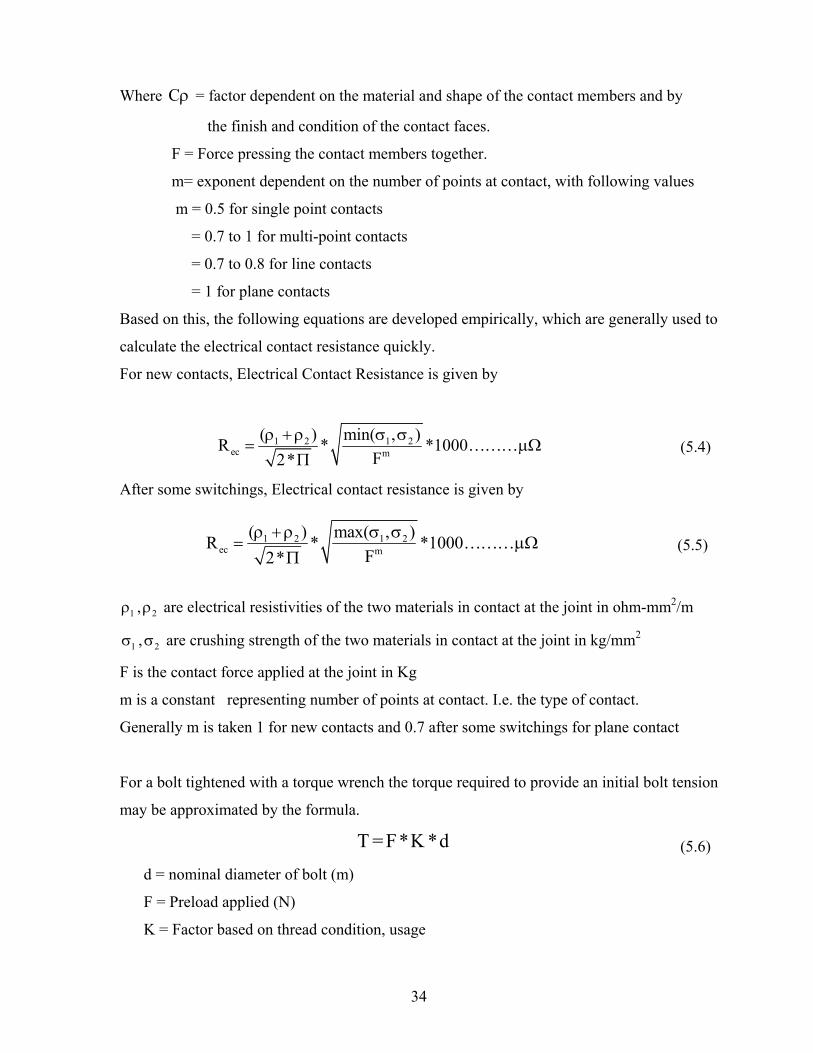
Where = factor dependent on the material and shape of the contact members and by Cρ

the finish and condition of the contact faces.

F = Force pressing the contact members together.

m= exponent dependent on the number of points at contact, with following values

m = 0.5 for single point contacts

= 0.7 to 1 for multi-point contacts

= 0.7 to 0.8 for line contacts

= 1 for plane contacts

Based on this, the following equations are developed empirically, which are generally used to

calculate the electrical contact resistance quickly.

For new contacts, Electrical Contact Resistance is given by

1 2 1 2ec m

( ) min( , )R * *1000F2*

ρ +ρ σ σ= μΩ

ΠKKK (5.4)

After some switchings, Electrical contact resistance is given by

1 2 1 2ec m

( ) max( , )R * *1000F2*

ρ +ρ σ σ= μ

ΠKKK Ω (5.5)

1ρ , are electrical resistivities of the two materials in contact at the joint in ohm-mm2ρ2/m

1σ , are crushing strength of the two materials in contact at the joint in kg/mm2σ2

F is the contact force applied at the joint in Kg

m is a constant representing number of points at contact. I.e. the type of contact.

Generally m is taken 1 for new contacts and 0.7 after some switchings for plane contact

For a bolt tightened with a torque wrench the torque required to provide an initial bolt tension

may be approximated by the formula.

(5.6) T = F*K *d

d = nominal diameter of bolt (m)

F = Preload applied (N)

K = Factor based on thread condition, usage

34

Typical K factors are tabulated as follows. Generally tightening torque corresponding to a

bolt size is taken form standard tables available in design data books.

Table5.1 K factor values

Steel Thread Condition K

As received, stainless on mild or alloy 0.30

As received, mild or alloy on same 0.20

Cadmium plated 0.16

Molybdenum-disulphide grease 0.14

PTFE lubrication 0.12

5.4 THERMAL CONTACT CONDUCTANCE

Thermal contact conductance plays an instrumental role for temperature drop across

the joint. It constricts the flow of heat across the joint contact surfaces because of reduced

contact area at the joint as shown in figure 5.3. The amount of actual contact area is also

dependent on the physical properties of the contacting materials. If one of the materials is

softer than the other, then the asperities of the harder material are likely to penetrate the

surface of the softer material and increase the contact area.

Figure 5.3 – Constriction of Heat Flow through an Interface formed by Two Materials.

At higher pressures, one would expect that the penetration of these asperities would increase.

In the case of materials of nearly the same hardness, the asperities would deform, and one

might expect that the amount of deformation would increase with pressure. Interfaces with a

higher mean thermal conductivity would be expected to have a lower resistance to heat

transfer than those interfaces that have lower mean thermal conductivities.

35

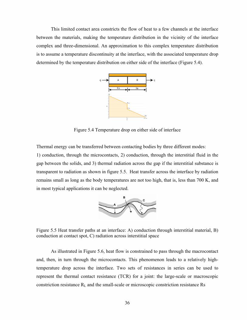
This limited contact area constricts the flow of heat to a few channels at the interface

between the materials, making the temperature distribution in the vicinity of the interface

complex and three-dimensional. An approximation to this complex temperature distribution

is to assume a temperature discontinuity at the interface, with the associated temperature drop

determined by the temperature distribution on either side of the interface (Figure 5.4).

Figure 5.4 Temperature drop on either side of interface

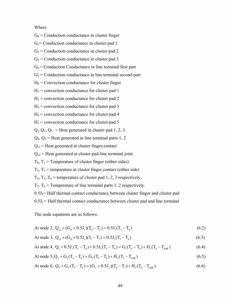
Thermal energy can be transferred between contacting bodies by three different modes:

1) conduction, through the microcontacts, 2) conduction, through the interstitial fluid in the

gap between the solids, and 3) thermal radiation across the gap if the interstitial substance is

transparent to radiation as shown in figure 5.5. Heat transfer across the interface by radiation

remains small as long as the body temperatures are not too high, that is, less than 700 K, and

in most typical applications it can be neglected.

Figure 5.5 Heat transfer paths at an interface: A) conduction through interstitial material, B) conduction at contact spot, C) radiation across interstitial space

As illustrated in Figure 5.6, heat flow is constrained to pass through the macrocontact

and, then, in turn through the microcontacts. This phenomenon leads to a relatively high-

temperature drop across the interface. Two sets of resistances in series can be used to

represent the thermal contact resistance (TCR) for a joint: the large-scale or macroscopic

constriction resistance RL and the small-scale or microscopic constriction resistance Rs

36

Figure 5.6 Thermal Resistance Network for nonconforming Rough Contacts

(5.7)

Many theoretical models for determining TCR have been developed for two

limiting cases: 1) conforming rough, here contacting surfaces are assumed to be perfectly flat

and 2) elasto constriction, where the effect of roughness is neglected, that is, contact of two

smooth spherical surfaces. These two limiting cases are simplified cases of real contacts

because engineering surfaces have both out of- flatness and roughness simultaneously. Few

analytical models for contact of two nonconforming rough surfaces exist in the literature.

Table 5.1 – Thermal Contact Conductance Models

correlation Condition Ross and Stoute

c cc 2 2

1 2

k .ph0.05H

2

=σ +σ

Modified flat contact model, some dependence on thermo-mechanical properties

Shlykov and Gamin go4 C C

c0 1

KK Ph 4.2*10d (345MPa)

=σ +σ2

+Modified flat contact model, some dependence

on thermo-mechanical properties

Cooper et,al 0.98

c

v

h P1.45Km H

⎡ ⎤σ= ⎢ ⎥

⎣ ⎦

Nominally flat, rough surfaces.

37

Yovanovich

0.95goc S

v a

Kh K m P1.25Km H Y

⎡ ⎤σ= +⎢ ⎥σ +α⎣ ⎦ β∧

Modification of Cooper,et al, rough surface

⎡ p v

p v

C / C 12C / C 1 Pr

⎤β = ⎢ ⎥

+⎢ ⎥⎣ ⎦

5.5 RELATION BASED ON THERMO-ELECTROMECHANICAL PROPERTIES

The above relations are developed in terms of thermo- mechanical properties. I.e. in

terms of mechanical properties like force at the joint area, surface roughness, hardness of the

contacting elements and thermal property like thermal conductivity. Empirical relation in

terms of thermo-electromechanical properties as electrical contact resistance is known is

given by

ectc __ __

RRK*

=λ

(5.8)

Generally air is entrapped between two asperities. To take care of conduction of heat through

the air gap in the voids, the thermal conductivity of the contacts has to be increased by a

factor of 2.1. So the thermal contact resistance is given by

ectc __ __

RRK* *2.1

=λ

(5.9)

Rec= Electrical contact resistance in micro-ohms __K is the average thermal conductivity of two different material in contact __λ is the average electrical resistivity of the two different material in contact

38

6. PROBLEM SOLVING PROCESS

6.1 PROBLEM DEFINITION

The problem has two parts. First part is to calculate steady state temperatures in

AKD-12 switch gear (frame 1and 3) by developing an analytical tool. Second part is to

predict the temperature variation in the switch gear for change in geometry of components.

As first part, an Excel tool is developed with Visual Basic backend, based on

thermal networking method to calculate steady state temperatures in electrical equipments.


for frame 1and 3. Test is conducted on AKD-12 switch gear –frame 1 and frame 3 under

continuous current to find out temperatures at different points along the current flow path.

Analytical results from the tool are then validated against the test data.

As second part, geometry of components in both the frames are varied and variation

in temperature at moving contact (highest temperature point) with respect to original

temperatures is observed.

Frame1 defines a switch gear through which 2000Amps current flows and

2000Amps circuit beaker is used. Frame 3 defines a switch gear through which 5000 Amps

current flows and the breaker assembled is 5000Amps rated air circuit breaker.

6.2 STEPS IN SOLVING THE PROBLEM

Steps followed to calculate temperatures analytically are listed below

1. Initially an electrical network diagram is developed for the switch gear considering all

the current flow paths and joints.

2. Electrical body resistance of each component and the corresponding joint resistance

are calculated.

3. The total calculated electrical resistance of the switch gear is compared with the

tested electrical resistance. Similarity of the two values replicates correctness of the

electrical network diagram.

39

4. Thermal network diagram is developed from the electrical network diagram.

5. Once the thermal network diagram is prepared, all the input parameters required for

“input and joints” sheets of the analytical tool are calculated.

6. Initial ‘h’ values are calculated based on natural convection correlations for vertical

and horizontal plate with constant wall temperature.

7. Following the sequence of steps in working with the analytical tool, steady state

temperatures at different point are obtained.

8. Further iterations are run with ‘h’ values corresponding to the temperatures obtained

from the first run to obtain accurate temperatures.

6.2.1 Electrical Network Diagram

As a first step, electrical network diagram is prepared. Fig 6.1 shows electrical

network diagram for AKD-12 frame 1 switch gear (For one phase). Components of the

switch gear are represented by their electrical body resistances and joints are represented by

electrical contact resistances. Resistances are arranged in series and parallel to replicate the

way current faces restriction to flow in the switch gear. Figure 6.2 represents electrical

network diagram for frame 3 (for single phase). Figure 6.3 shows electrical network diagram

for frame3 with three phases.

40

Figure 6.1

41

Figure 6.2

42

Figure 6.3

43

6.2.2 Electrical Resistance Calculation

In this step, electrical resistance of the electrical network diagram is calculated which

involves calculation of body resistances of components and contact resistance of joints. From

the geometry of the components, body resistance (DC electrical resistance) is calculated

using the formula LRAρ

= (6.1)

Joint resistance of bolted joint is calculated knowing the bolting torque or force and

number of bolts using the contact resistance tool. Resistance at contacts held by spring

loading is calculated based on spring force acting at the contact. (Details in chapter 5)

Following shows resistance calculation for AKD 12 frame 1 Global Air Circuit Breaker

portion

Force applied at each cluster finger contact tip = 55 N. From the Excel Contact

resistance calculation tool, contact resistance is 35.3 micro-ohms for 55 N. There are 18 such

contact point i.e. 18 resistances connected in parallel. So equivalent cluster contact resistance

=35.3 1.9618

= μ −Ω

1. Equivalent Resistance of cluster assembly (both sides) = 2.1 micro –ohms

2. Body resistance of cluster pad = 0.72 micro –ohms

3. Joint resistance between cluster pad and load terminal = 0.65 micro-ohms

4. Load terminal body resistance =1.53 micro –ohms

5. Resistance of flexible conductor, moving conductor, moving contact and their joint

(Considering 300 N spring force at each moving contact) =12.9micro-ohms

6. Line terminal body resistance =1.24 micro-ohms

7. Joint resistance at line terminal and cluster pad =0.65 micro-ohms

8. Body resistance of cluster pad =0.72 micro –ohms

9. Equivalent Resistance of cluster assembly =2.1 micro –ohms

Total Breaker resistance calculated by excel tool= 22.6micro –ohms

44

6.2.3 Comparison with Measured Value

In this step, electrical resistance from analytical calculations is compared with the

resistance value from test data to validate the correctness of the electrical network diagram.

Breaker resistance calculated by excel tool= 22.6micro –ohms

Resistance from Test =19 micro –ohms

While calculating body resistance of flexible conductor, it is considered as solid

conductor though it is made of laminates pressed together. This may be the major cause for

3.6 micro-ohms difference between the analytical and test value. In the same way, electrical

resistance is calculated for the entire switch gear and compared with test data. Comparing

electrical resistances is very important, as similarity of both the results indicates the

correctness of the electrical network diagram and based on this diagram all the remaining

work is carried out.

6.2.4 Thermal Network Diagram

The next step is to draw thermal network diagram based on electrical network

diagram. It is drawn considering conduction, convection resistances, thermal contact

resistances at joints and heat generators. Figure6.4 shows thermal network diagram for Frame

1(for one phase only). It has 143 nodes, out of which 5 nodes represent air in the

compartment of switch gear. Figure 6.5 shows thermal network diagram for frame 3. Each

node is connected to the other with a thermal conductor maintaining continuity through out

the network. Frame 3 has 658 nodes with 208 nodes for each phase. Black node represents a

component; red node represents a joint, blue node represents air. Green conductor represents

conduction resistance, blue conductor represents convection resistance and red conductor

represents half the thermal contact resistance. Heat generated by I2R loss in the component is

represented by black arrow, heat generation at joint by red arrow. Single component is

represented as more than one node depending on the length of the component. A node is

considered at each joint and a new node is considered wherever cross section changes.

45

Figure6.4

46

Figure 6.5

47

6.2.4(a) Node Equations

Now equations are developed at every node seen in the thermal network diagram.

Node equations for cluster pad portion are written as follows. Thermal network diagram

shows contact between cluster finger and cluster pad, cluster pad, joint between cluster pad

and line terminal and line terminal. Nodes 0, 1 represent cluster fingers. Nodes 2, 3 represent

cluster finger contact. The network diagram is as shown in figure 5.6. Cluster pad has 3

different cross-sections, so 3 nodes are considered (Nodes 4, 5, 6). Line terminal is divided

into two parts, so two nodes are considered (Nodes 8, 9).

Figure 6.6Thermal Network Diagram for cluster pad region

48

Where

G0 = Conduction conductance in cluster finger

G1= Conduction conductance in cluster pad 1

G2 = Conduction conductance in cluster pad 2


G4 = Conduction Conductance in line terminal first part

G5 = Conduction conductance in line terminal second part

H0 = Convection conductance for cluster finger

H1 = convection conductance for cluster pad 1





Q1, Q2, Q3 = Heat generated in cluster pad 1, 2, 3.

Q4, Q5 = Heat generated in line terminal parts 1, 2

Qc1 = Heat generated at cluster finger contact

Qc2 = Heat generated at cluster pad-line terminal joint

T0, T1 = Temperature of cluster finger (either sides)

T2, T3 = temperature at cluster finger contact (either side)

T4, T5, T6 = temperature of cluster pad 1, 2, 3 respectively.

T7, T8 = Temperature of line terminal parts 1, 2 respectively.

0.5J1= Half thermal contact conductance between cluster finger and cluster pad

0.5J2 = Half thermal contact conductance between cluster pad and line terminal

The node equations are as follows:

At node 2, (6.2) c1 0 1 0 2 1 2 4Q (G 0.5J )(T T ) 0.5J (T T )+ + − = −


At node 4, (6.4) 1 1 2 4 1 3 4 1 4 5 1 4 AIQ 0.5J (T T ) 0.5J (T T ) G (T T ) H (T T )+ − + − = − + − R

At node 5, (6.5) 2 1 4 5 2 5 6 2 5 AIRQ G (T T ) G (T T ) H (T T )+ − = − + −

At node 6, (6.6) 3 2 5 6 3 2 6 7 3 6 AIRQ G (T T ) (G 0.5J )(T T ) H (T T )+ − = + − + −

49


At node 8, (6.8) 4 2 7 8 4 8 9 4 8 AIQ 0.5J (T T ) (G )(T T ) H (T T+ − = − + − R )

6.2.5 Calculation of Input Parameters

In this step, all the input parameters required for the calculation of conduction,

conductance, convection conductance, I2R heat generated in the components and joints,

convective heat transfer coefficient, electrical and thermal contact resistances are calculated.

Input parameters required are current, electrical resistivity, thermal conductivity, geometry of

the components, joint forces etc. (Described in detail at section 6.3.1)

6.2.6 Convective Heat Transfer Coefficient Calculation

Convective heat transfer co-efficient (h) values are calculated based on correlations

for isothermal vertical plate and horizontal plate with natural convection. Initial film

temperature is calculated based on approximate temperature the component would reach. By

standards, temperature rise should not exceed 850C for any component in the switch gear.

Maximum temperature in gear region is limited to 650C. Correlations used in calculating ‘h’

are given at section 4.12.1(a), (b).

6.3 ANALYTICAL TOOL TO CALCULATE TEMPERATURES

An analytical tool is developed with Excel interface and Visual basic back up to

calculate steady state temperatures. The solver method followed is Gauss elimination method.

Nodal equations are developed at each node and the linear equations are solved by

multiplying the inverse of temperature co-efficient matrix with heat column matrix to obtain

the temperatures. The tool is considered as five worksheets, out of which 2 are input sheets.

They are:

1. Input Sheet

2. Joints sheet

3. Nodes Sheet

4. Network Sheet

5. Output Sheet

50

6.3.1 Input Sheet

Snap shot of input sheet is shown in figure 6.7. Input sheet contains four tables—

input parameters table, ‘h’ table for vertical plate, ‘h’ table for horizontal plate and geometry

of the components table. Input for input parameters table are –current, electrical resistivity

and thermal conductivity. Inputs for ‘h’ tables are air temperature, plate temperature and

plate width, height. Selection of ‘h’ table depends on position of plate considered whether

placed vertically or horizontally (whether cooling is on top surface or lower surface). Input

for geometry of components table are component length, width , thickness, number of nodes,

h value calculated from h table and surface area. Surface area is given as input to allow the

user to enter the value depending on the actual area subjected to air flow. Input columns are

represented by green color and values calculated by yellow color. Upon clicking compute

button, length per node, cross sectional area, heat generated, conduction and convection

conductances are calculated. Upon clicking “clear this sheet” button all the vales entered the

sheet are cleared. Upon clicking “clear all sheets button”, entire data in all sheets is deleted

and this is used when starting a new problem.

51

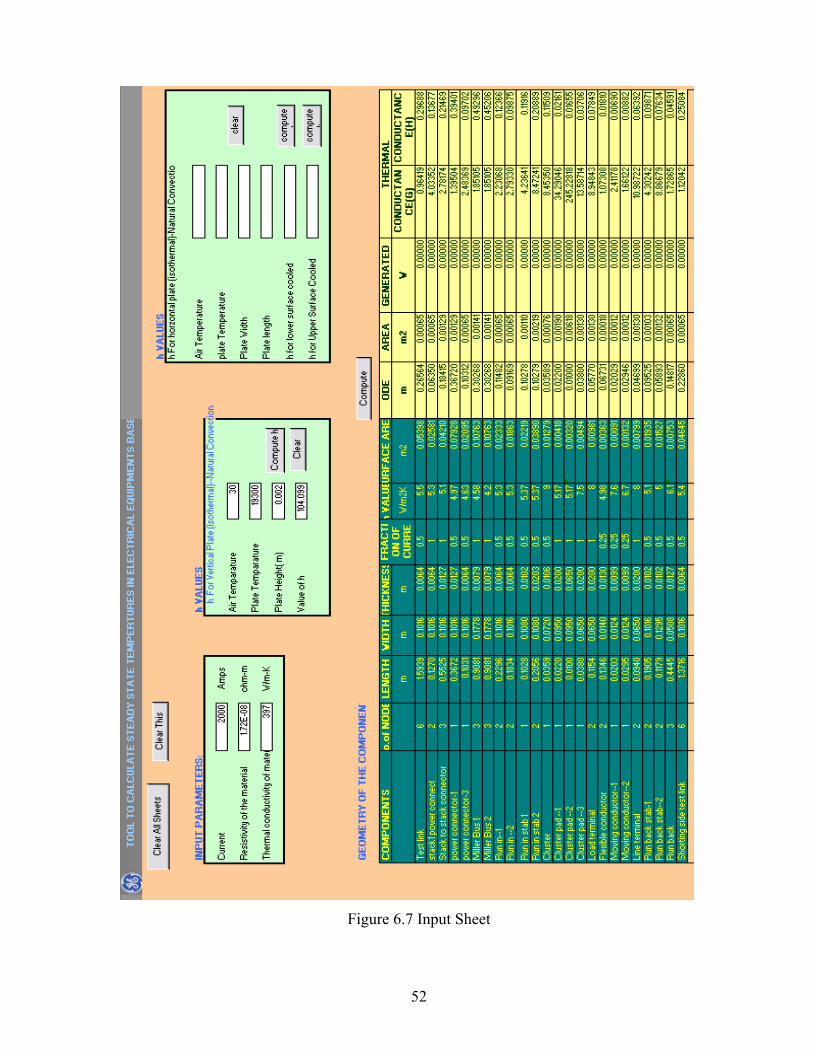
Figure 6.7 Input Sheet

52

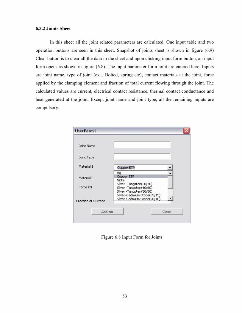
6.3.2 Joints Sheet

In this sheet all the joint related parameters are calculated. One input table and two

operation buttons are seen in this sheet. Snapshot of joints sheet is shown in figure (6.9)

Clear button is to clear all the data in the sheet and upon clicking input form button, an input

form opens as shown in figure (6.8). The input parameter for a joint are entered here. Inputs

are joint name, type of joint (ex... Bolted, spring etc), contact materials at the joint, force

applied by the clamping element and fraction of total current flowing through the joint. The

calculated values are current, electrical contact resistance, thermal contact conductance and

heat generated at the joint. Except joint name and joint type, all the remaining inputs are

compulsory.

Figure 6.8 Input Form for Joints

53

Figure 6.9 Joints Sheet

54

6.3.3 Nodes Sheet

In nodes sheet, all the nodes are entered in a sequence as per the numbering given in

the thermal network diagram. Snap shot of nodes sheet is shown in figure (6.11). In the sheet

seen is a nodes table, clear sheet button and add nodes button. Upon clicking add nodes

button, an input form drops down as shown in figure (6.10). It contains many options like

component, joint, air and dummy node. Only one can be chosen at a time. Upon choosing an

option, corresponding input form is activated. By choosing components radio button,

particular component can be selected form the drop down menu and click add component

button to add to the nodes sheet. Similarly joint nodes, air nodes and dummy nodes can be

added to the nodes sheet. Dummy nodes are imaginary nodes used at branching and joining

of resistances. It does have zero values for the thermal properties. Generally air nodes are

entered at the end and air temperature input option is compulsory.

Figure 6.10 Input Form for Nodes

55

Figure 6.11 Nodes Sheet

The user must observe that upon changing any values in the previous two sheets,

values are not updated in this sheet. The user has to manually update this sheet by deleting

corresponding rows or by clearing the sheet and adding nodes again by clicking the add

nodes button. No row can be left unfilled between two filled rows. Row with no elements is

considered as end of the nodes table.

56

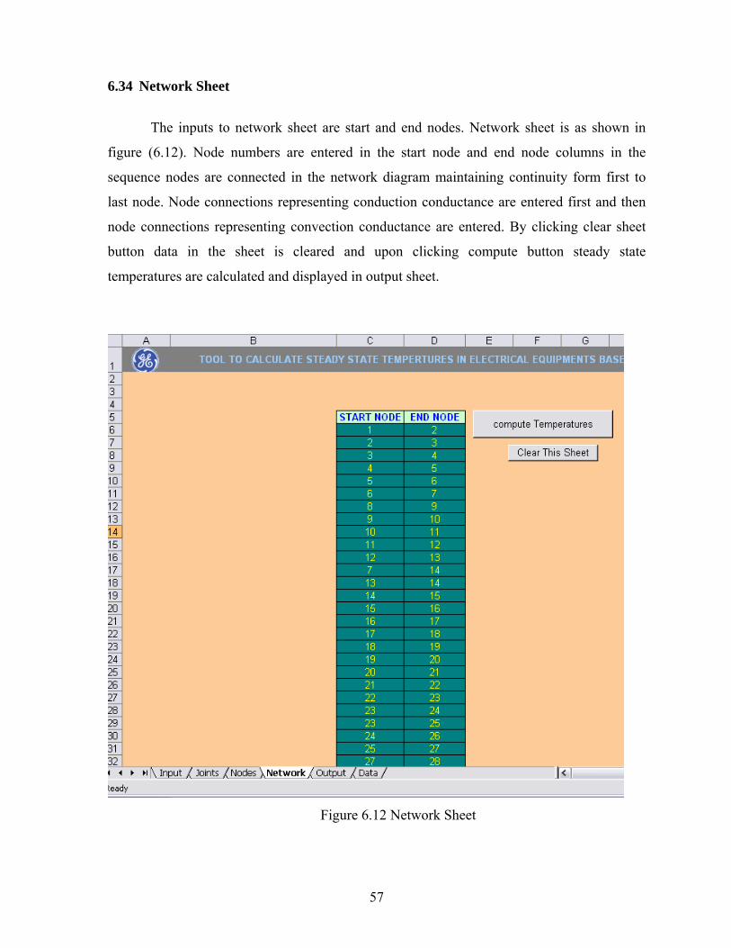
6.34 Network Sheet

The inputs to network sheet are start and end nodes. Network sheet is as shown in

figure (6.12). Node numbers are entered in the start node and end node columns in the

sequence nodes are connected in the network diagram maintaining continuity form first to

last node. Node connections representing conduction conductance are entered first and then

node connections representing convection conductance are entered. By clicking clear sheet

button data in the sheet is cleared and upon clicking compute button steady state

temperatures are calculated and displayed in output sheet.

Figure 6.12 Network Sheet

57

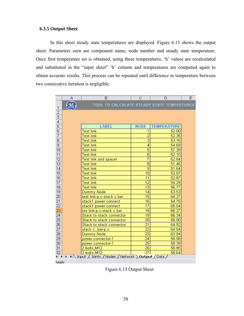
6.3.5 Output Sheet

In this sheet steady state temperatures are displayed. Figure 6.13 shows the output

sheet. Parameters seen are component name, node number and steady state temperature.

Once first temperature set is obtained, using these temperatures, ‘h’ values are recalculated

and substituted in the “input sheet” ‘h’ column and temperatures are computed again to

obtain accurate results. This process can be repeated until difference in temperature between

two consecutive iteration is negligible.

Figure 6.13 Output Sheet

58

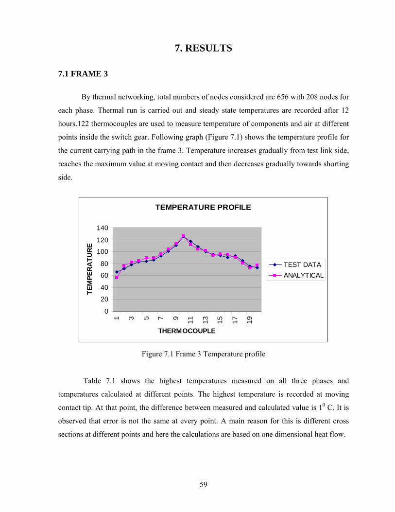
7. RESULTS

7.1 FRAME 3

By thermal networking, total numbers of nodes considered are 656 with 208 nodes for

each phase. Thermal run is carried out and steady state temperatures are recorded after 12

hours.122 thermocouples are used to measure temperature of components and air at different

points inside the switch gear. Following graph (Figure 7.1) shows the temperature profile for

the current carrying path in the frame 3. Temperature increases gradually from test link side,

reaches the maximum value at moving contact and then decreases gradually towards shorting

side.

TEMPERATURE PROFILE

0

20

40

60

80

100

120

140

1 3 5 7 9 11 13 15 17 19

THERMOCOUPLE

TEM

PER

ATU

RE

TEST DATAANALYTICAL

Figure 7.1 Frame 3 Temperature profile

Table 7.1 shows the highest temperatures measured on all three phases and

temperatures calculated at different points. The highest temperature is recorded at moving

contact tip. At that point, the difference between measured and calculated value is 10 C. It is

observed that error is not the same at every point. A main reason for this is different cross

sections at different points and here the calculations are based on one dimensional heat flow.

59

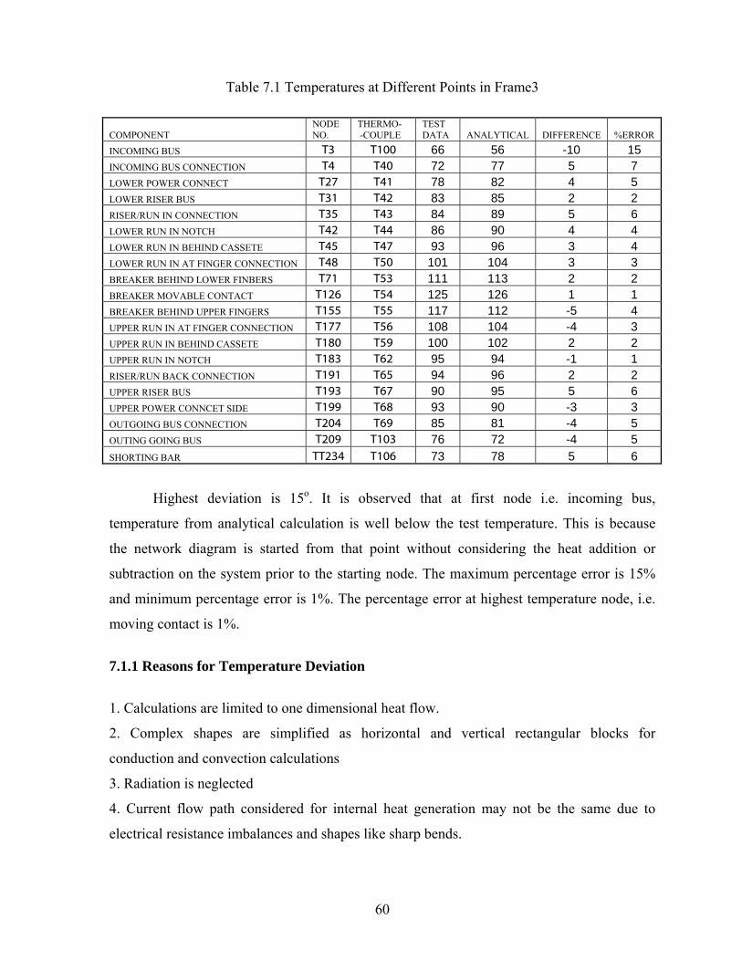
Table 7.1 Temperatures at Different Points in Frame3

COMPONENT NODE NO.

THERMO- -COUPLE

TEST DATA ANALYTICAL DIFFERENCE %ERROR

INCOMING BUS T3 T100 66 56 -10 15 INCOMING BUS CONNECTION T4 T40 72 77 5 7 LOWER POWER CONNECT T27 T41 78 82 4 5 LOWER RISER BUS T31 T42 83 85 2 2 RISER/RUN IN CONNECTION T35 T43 84 89 5 6 LOWER RUN IN NOTCH T42 T44 86 90 4 4 LOWER RUN IN BEHIND CASSETE T45 T47 93 96 3 4 LOWER RUN IN AT FINGER CONNECTION T48 T50 101 104 3 3 BREAKER BEHIND LOWER FINBERS T71 T53 111 113 2 2 BREAKER MOVABLE CONTACT T126 T54 125 126 1 1 BREAKER BEHIND UPPER FINGERS T155 T55 117 112 -5 4 UPPER RUN IN AT FINGER CONNECTION T177 T56 108 104 -4 3 UPPER RUN IN BEHIND CASSETE T180 T59 100 102 2 2 UPPER RUN IN NOTCH T183 T62 95 94 -1 1 RISER/RUN BACK CONNECTION T191 T65 94 96 2 2 UPPER RISER BUS T193 T67 90 95 5 6 UPPER POWER CONNCET SIDE T199 T68 93 90 -3 3 OUTGOING BUS CONNECTION T204 T69 85 81 -4 5 OUTING GOING BUS T209 T103 76 72 -4 5 SHORTING BAR TT234 T106 73 78 5 6

Highest deviation is 15o. It is observed that at first node i.e. incoming bus,

temperature from analytical calculation is well below the test temperature. This is because

the network diagram is started from that point without considering the heat addition or

subtraction on the system prior to the starting node. The maximum percentage error is 15%

and minimum percentage error is 1%. The percentage error at highest temperature node, i.e.

moving contact is 1%.

7.1.1 Reasons for Temperature Deviation

1. Calculations are limited to one dimensional heat flow.

2. Complex shapes are simplified as horizontal and vertical rectangular blocks for

conduction and convection calculations

3. Radiation is neglected

4. Current flow path considered for internal heat generation may not be the same due to

electrical resistance imbalances and shapes like sharp bends.

60

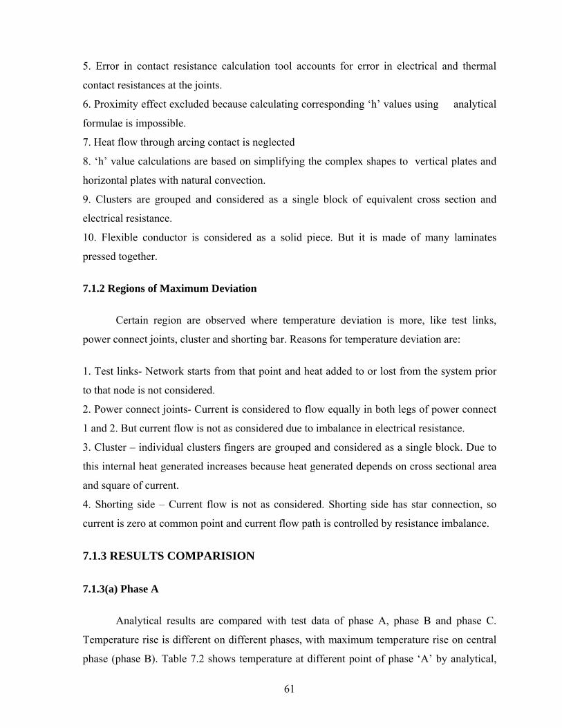
5. Error in contact resistance calculation tool accounts for error in electrical and thermal

contact resistances at the joints.

6. Proximity effect excluded because calculating corresponding ‘h’ values using analytical

formulae is impossible.

7. Heat flow through arcing contact is neglected

8. ‘h’ value calculations are based on simplifying the complex shapes to vertical plates and

horizontal plates with natural convection.

9. Clusters are grouped and considered as a single block of equivalent cross section and

electrical resistance.

10. Flexible conductor is considered as a solid piece. But it is made of many laminates

pressed together.

7.1.2 Regions of Maximum Deviation

Certain region are observed where temperature deviation is more, like test links,

power connect joints, cluster and shorting bar. Reasons for temperature deviation are:

1. Test links- Network starts from that point and heat added to or lost from the system prior

to that node is not considered.

2. Power connect joints- Current is considered to flow equally in both legs of power connect

1 and 2. But current flow is not as considered due to imbalance in electrical resistance.

3. Cluster – individual clusters fingers are grouped and considered as a single block. Due to

this internal heat generated increases because heat generated depends on cross sectional area

and square of current.

4. Shorting side – Current flow is not as considered. Shorting side has star connection, so

current is zero at common point and current flow path is controlled by resistance imbalance.

7.1.3 RESULTS COMPARISION

7.1.3(a) Phase A

Analytical results are compared with test data of phase A, phase B and phase C.

Temperature rise is different on different phases, with maximum temperature rise on central

phase (phase B). Table 7.2 shows temperature at different point of phase ‘A’ by analytical,

61

CFD and experiment. (CFD results are from Analysis Team). Graph 7.2 shows temperature

profile for phase A. Analytical, CFD results and experimental values are compared in the

graph. Analytical results are on higher side and CFD results are on lower side compared to

test results. At same points on similar components temperature difference is observed in test

data due to proximity effect, as observed at thermocouples 14, 15, 16. But analytical values

show the same temperature for all those three points as proximity effect is not considered.

Figure 7.3 shown temperature profile of phase A without considering proximity effect.

Table 7.2 Temperatures on Phase A

PHASE A T.C. ANALYTICAL TEST DATA CFD

COMPONENT Incoming bus connection 10 77 69 67 Lower PC side 11 78 75 66 Middle of lower riser bus 12 86 79 66 Riser/run in connection 13 89 80 66 Lower run in notch-left 14 90 79 68 Lower run in notch-center 15 90 83 68 Lower run in notch-right 16 90 87 68 Lower run in behind cassete- left 17 96 83 81 Lower run in behind cassete- center 18 96 86 82 Lower run in behind cassete- right 19 96 93 81 Lower run in at finger connection- left 20 104 92 101 Lower run in at finger connection- center 21 104 95 101 Lower run in at finger connection- right 22 104 101 101 Breaker behind lower fingers 23 113 108 103 Breaker movable contacts 24 126 125 115 Breaker behind upper fingers 25 112 113 113 Upper run in at finger connection- left 26 104 106 110 Upper run in at finger connection- center 27 104 101 111 Upper run in at finger connection- right 28 104 97 111 Upper run in behind cassete- left 29 102 84 89 Upper run in behind cassete- center 30 102 93 91 Upper run in behind cassete- right 31 102 96 90 Upper run in notch-left 32 94 82 77 Upper run in notch-center 33 94 86 78 Upper run in notch-right 34 94 92 77 Riser/run in connection- left 35 96 76 72 Riser/run in connection- right 36 96 90 72 Middle of upper riser bus 37 94 89 72 Upper PC side 38 90 88 78 Outgoing bus connection 39 81 81 80

62

TEMP. PLOT FOR PHASE A

0

20

40

60

80

100

120

140

1 3 5 7 9 11 13 15 17 19 21 23 25 27 29

THERMOCOUPLES

TEM

P ANALYTICALEXPCFD

Figure 7.2 Temperatures Comparison for Phase A

phase A

0

20

40

60

80

100

120

140

1 3 5 7 9 11 13 15 17

thermpcouples

tem

pera

ture

analyticalexperimental

Figure 7.3 Temperatures Comparison without Proximity Effect

7.1.3(b) Phase B

Out of all three phases, maximum temperature is observed on this phase. Graph 7.4

shows temperature profile for phase B corresponding to similar point on phase A. The

analytical values match better with test data as the proximity effect is less in the central phase.

Graph 7.5 shows temperature profile without considering proximity effect.

63

TEMP. PLOT FOR PHASE B

0

20

40

60

80

100

120

140

1 3 5 7 9 11 13 15 17 19 21 23 25 27 29

THERMOCOUPLES

TEM

P ANALYTICALEXPCFD

Figure 7.4 Temperatures comparison for phase B

phase B

0

20

40

60

80

100

120

140

1 3 5 7 9 11 13 15 17

thermocouples

tem

pera

ture

analyticalexperimantal

Figure 7.5 Temperatures comparison without Proximity Effect

64

7.1.3(c) Phase C

Graph 7.6shows temperature profile for phase C .Here deviation is observed to be

more. Graph 7.7 shows temperature profile for phase C without considering proximity effect.

TEMP. PLOT FOR PHASE C

0

20

40

60

80

100

120

140

1 2 3 4 5 6 7 8 9101112131415161718192021222324252627282930

THERMOCOUPLES

TEM

PER

ATU

RE

analyticalExperimentalCFD

Figure 7.6 Temperatures comparison for phase C

phase c

0.000

20.000

40.000

60.000

80.000

100.000

120.000

140.000

1 3 5 7 9 11 13 15 17

thermocouple

tem

pera

ture

experimtalanalytical


65

7.1.4 TEMPERATURE PREDICTION

By changing different parameters, the change in temperatures and temperature profile

are observed. This gives an insight into how different input parameters affect the

temperatures of different components.

7.1.4(a) Change in Run-In Geometry

Dimensions of run-in and run-back are changed to predict the temperature change at

highest temperature, .i.e. moving contact. Table 7.3 shows the actual values and changed

geometry of run-ins. It is observed that with new geometry, temperature at moving contact

decreases by 100C.

Table 7.3 Run-In Geometry

CASE-1 ACTUAL VALUES (m) COMPONENT WIDTH THICKNESS LENGTH

Run in--part—1(One Strip) 0.1524 0.00635 0.234 part--2 0.1778 0.00635 0.1092 part--3 0.1524 0.00635 0.209 part--4 0.1016 0.00635 0.159 Part--5 0.0944 0.00635 0.05 CASE-1 CHANGED VALUES (m)

COMPONENT WIDTH THICKNESS LENGTH Run in--part—1(One Strip) 0.1016 0.02921 0.1206 part--2 0.127 0.01905 0.2159 part--3 0.127 0.01905 0.2159 part--4 0.1016 0.01905 0.104775 Part--5 0.1016 0.01905 0.104775

Table 7.4 Analytical Temperatures with and without Change in Run-In Dimensions

COMPONENT NAME ANALY.TEMP. BEFORE AFTER DIFF. INCOMING BUS 56 56 0 INCOMING BUS CONNECTION 77 77 0 LOWER POWER CONNECT SIDE 78 78 0 LOWER POWER CONNECT 82 81 1 LOWER RISER BUS 83 82 1

66

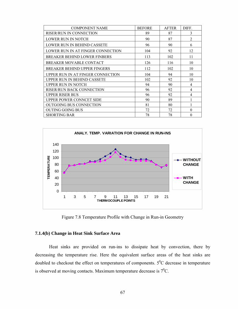
COMPONENT NAME BEFORE AFTER DIFF. RISER/RUN IN CONNECTION 89 87 3 LOWER RUN IN NOTCH 90 87 2 LOWER RUN IN BEHIND CASSETE 96 90 6 LOWER RUN IN AT FINGER CONNECTION 104 92 12 BREAKER BEHIND LOWER FINBERS 113 102 11 BREAKER MOVABLE CONTACT 126 116 10 BREAKER BEHIND UPPER FINGERS 112 102 10 UPPER RUN IN AT FINGER CONNECTION 104 94 10 UPPER RUN IN BEHIND CASSETE 102 92 10 UPPER RUN IN NOTCH 94 90 4 RISER/RUN BACK CONNECTION 96 92 4 UPPER RISER BUS 96 92 4 UPPER POWER CONNCET SIDE 90 89 1 OUTGOING BUS CONNECTION 81 80 1 OUTING GOING BUS 72 72 0 SHORTING BAR 78 78 0

ANALY. TEMP. VARIATION FOR CHANGE IN RUN-INS

0

20

40

60

80

100

120

140

1 3 5 7 9 11 13 15 17 19 21THERMOCOUPLE POINTS

TEM

PER

ATU

RE

WITHOUTCHANGE

WITHCHANGE

Figure 7.8 Temperature Profile with Change in Run-in Geometry

7.1.4(b) Change in Heat Sink Surface Area

Heat sinks are provided on run-ins to dissipate heat by convection, there by

decreasing the temperature rise. Here the equivalent surface areas of the heat sinks are

doubled to checkout the effect on temperatures of components. 50C decrease in temperature

is observed at moving contacts. Maximum temperature decrease is 70C.

67

Table 7.5 Analytical Temperatures Comparison by Doubling the Heat Sink Surface Area

COMPONENT NAME ANALY.TEMP.

BEFORE AFTER DIFF. INCOMING BUS 56 56 0 INCOMING BUS CONNECTION 77 76 1 LOWER POWER CONNECT SIDE 78 78 1 LOWER POWER CONNECT 82 81 1 LOWER RISER BUS 83 81 2 RISER/RUN IN CONNECTION 89 84 5 LOWER RUN IN NOTCH 90 83 6 LOWER RUN IN BEHIND CASSETE 96 91 6 LOWER RUN IN AT FINGER CONNECTION 104 100 5 BREAKER BEHIND LOWER FINBERS 113 109 4 BREAKER MOVABLE CONTACT 126 122 5 BREAKER BEHIND UPPER FINGERS 112 106 6 UPPER RUN IN AT FINGER CONNECTION 104 98 6 UPPER RUN IN BEHIND CASSETE 102 95 6 UPPER RUN IN NOTCH 94 87 7 RISER/RUN BACK CONNECTION 96 92 4 UPPER RISER BUS 96 92 4 UPPER POWER CONNCET SIDE 90 89 1 OUTGOING BUS CONNECTION 81 80 1

OUTING GOING BUS 72 72 0 SHORTING BAR 78 78 0

ANALY. TEMP. VARIATION BOUBLING HEAT SINK SURFACE AREA

0

20

40

60

80

100

120

140


TEM

PER

ATU

RE

WITHOUTCHANGE

WITHCHANGE

56

Figure7.9 Temperature Variation by Doubling Surface Area

68

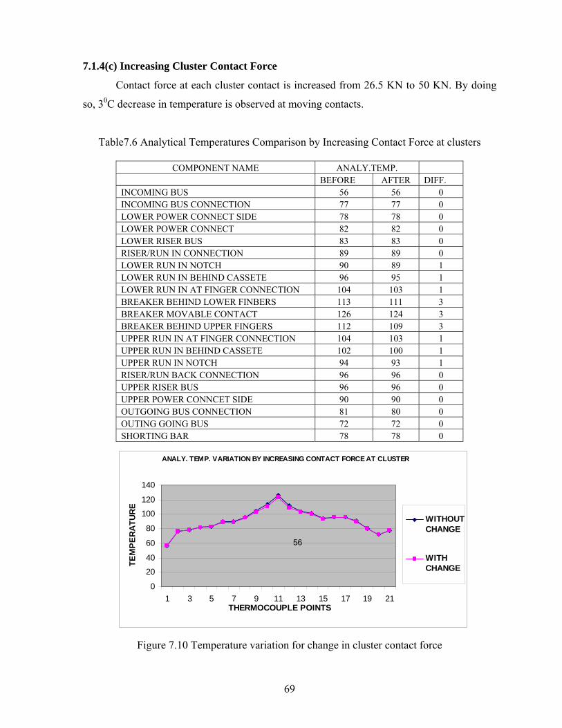
7.1.4(c) Increasing Cluster Contact Force

Contact force at each cluster contact is increased from 26.5 KN to 50 KN. By doing

so, 30C decrease in temperature is observed at moving contacts.

Table7.6 Analytical Temperatures Comparison by Increasing Contact Force at clusters

COMPONENT NAME ANALY.TEMP. BEFORE AFTER DIFF. INCOMING BUS 56 56 0 INCOMING BUS CONNECTION 77 77 0 LOWER POWER CONNECT SIDE 78 78 0 LOWER POWER CONNECT 82 82 0 LOWER RISER BUS 83 83 0 RISER/RUN IN CONNECTION 89 89 0 LOWER RUN IN NOTCH 90 89 1 LOWER RUN IN BEHIND CASSETE 96 95 1 LOWER RUN IN AT FINGER CONNECTION 104 103 1 BREAKER BEHIND LOWER FINBERS 113 111 3 BREAKER MOVABLE CONTACT 126 124 3 BREAKER BEHIND UPPER FINGERS 112 109 3 UPPER RUN IN AT FINGER CONNECTION 104 103 1 UPPER RUN IN BEHIND CASSETE 102 100 1 UPPER RUN IN NOTCH 94 93 1 RISER/RUN BACK CONNECTION 96 96 0 UPPER RISER BUS 96 96 0 UPPER POWER CONNCET SIDE 90 90 0 OUTGOING BUS CONNECTION 81 80 0 OUTING GOING BUS 72 72 0 SHORTING BAR 78 78 0

ANALY. TEMP. VARIATION BY INCREASING CONTACT FORCE AT CLUSTER

0

20

40

60

80

100

120

140


TEM

PER

ATUR

E

WITHOUTCHANGE

WITHCHANGE

56

Figure 7.10 Temperature variation for change in cluster contact force

69

7.2 FRAME 1

By thermal networking method, current flowing path in frame 1 is considered as 138

nodes. 5 nodes are considered for air. Steady state temperatures are calculated analytically

using the analytical tool. Thermal run is carried out and steady state temperatures are

recorded after 12 hours. Analytical and experimental values at different points are tabulated

as shown in table 7.7.

Table 7.7 Temperatures for Frame1

TEST

TEMPERATURE ANALYTICAL DIFF. %

ERROR LABEL RISE TOTAL TOTAL

Test link 37 64 62.10 -1.9 2.97 Stack to stack bar joint 30 57 64.54 7.5 13.22 Power connect 26 53 58.58 5.6 10.53 Miller bus-middle 40 67 72.00 5.0 7.47 miller bus- End 56 83 82.60 -0.4 0.48 Run-in stab 57 84 86.83 2.8 3.37 Lower terminal(line) 78 105 109.87 4.9 4.64 Moving contact 94 121 129.06 8.1 6.66 Top terminal ( load) 74 101 106.85 5.9 5.80 Runback Stab 62 89 91.71 2.7 3.04 Runback stab-test link joint 54 81 81.51 0.5 0.63 Shorting side test link 42 69 64.87 -4.1 5.99

Maximum temperature deviation is 8.10 and minimum 0.40C. The maximum

percentage error is 13.2% and minimum percentage error is 0.48%. At moving contact, i.e.

the maximum temperature node, temperature deviation is 8.10C giving 6.7 % error. Graph

7.11 shows the temperature profile of frame1. Analytical temperatures at start node and end

node are lower than the experimental values while at all other nodes analytical values are

more than experimental values. This is because the network diagram is started from

particular point and effect of heat addition or loss on the system prior to that node is not

considered. The temperatures calculated analytically are for single phase only but in actual

70

testing condition, all three phases are considered and so the node at the shorting side node, i.e.

the end node differs.

Figure 6.8 Temperatures comparison for frame1

FRAME-1 TEMPERATURE PROFILE

0.00

20.00

40.00

60.00

80.00

100.00

120.00

140.00

1 2 3 4 5 6 7 8 9 10 11 12

THERMOCOUPLE POINTS

TEM

PERA

TURE

analyticaltest

Figure 7.11 Frame -1 Temperature Profile

71

8. CONCLUSION AND FURTHER WORK

The aim of this work is to develop an analytical tool to calculate steady state

temperatures in electrical equipments and predict the temperature variation with change in

geometry of the components in the equipment, particularly with switch gear. This chapter

summarizes the contribution, conclusion of the work and proposes ideas for further work.

8.1 CONTRIBUTION

An analytical tool is developed to calculate contact resistances at joints in current

carrying paths. This tool is suitable to calculate electrical and thermal contact resistances at

bolted joints and spring loaded contacts with different types of contact materials at contact

tips.

An analytical tool is developed to calculate convective heat transfer co-efficient in

natural convection. This tool is useful to calculate ‘h’ values for isothermal vertical and

horizontal plates in natural convection.

An analytical tool is developed to calculate steady state temperatures in current

carrying paths. This tool is useful to calculate steady state temperatures in electrical

equipment and it is validated with AKD-12 –Frame 1 and Frame3 thermal run data. Above

mentioned two tools are used in this tool.

Temperature prediction work is carried out by changing input parameters in the

switch gears to observe its effect on temperatures of different components.

8.2 CONCLUSION

Comparing the results from analytical tool and experimental data, it can be concluded

that the analytical tool can be used to calculate steady state temperatures and to have an idea

of temperature profile along the current carrying path in electrical equipment.

Comparing the test data and analytical results, good matching is observed in the

temperature profiles. Deviation is much at few points like starting nodes and ending nodes.

72

The maximum percentage error in frame 1 is 13%. The percentage error at point of interest

i.e. at moving contact is 6.7%. The maximum percentage error for frame 3 is 15% and at

moving contact, it is 1 %. For change in run-in geometry, 100C temperature decrease is

observed. Change in cluster contact force doesn’t have much effect on temperatures.

By analyzing the results, it can be concluded that thermal network theory helps

engineers to predict temperatures easily for changes in design reducing design cycle time and

it is flexible as to expand its application to any heat generating equipment.

8.3 FURTHER WORK

The following are the suggestions for further investigation

• In the current project work, initial ‘h’ values are calculated based on some reliable data

giving the temperatures the components would reach. Using those ‘h’ values,

temperatures are found out using the analytical tool. Based on these temperatures, ‘h’

values are calculated and temperatures are found out again. This is carried out manually

till the difference between temperatures from two successive iterations is small. So logic

has to be included in the tool to do the iteration work by itself.

• In the work done , for calculating temperatures of components placed in a closed

compartment like switch gears, temperature of air inside the compartment is taken as

input as components are placed at different distances form the compartment walls.

Further work has to be done to avoid considering temperature of air in the compartment

as input parameter.

• Error is not same at every point, so applying correction factor has become tricky. Further

work has to be carried out to identify the pockets and apply correction factor accordingly.

• In the present work, radiation effect is neglected as the maximum temperature rise is

850C and to avoid the complexity in building network. Further investigation may be done

to include radiation in the thermal network to take care of problems involving higher

temperatures.

73

9. REFERENCES

[1] Peter U. Frei and Hans O. Weichert, “Advanced thermal simulation of a circuit breaker”

in 0-7803-8460-1/04

[2] IEEE Correspondence--“A practical Method of Heat Computation in Electronic

Equipment” in IEEE transaction on parts, Materials and Packing, 2002

[3] Hiroshi Okashita and Kazunori Fukuya “Low Voltage Air Circuit Breaker Type AE-SW

Series” in Mitsubishi Electric Advance, June2005

[4] Lionel Boyer “Contact Resistance Calculation: Generalization of Greenwood’s Formula

Including Interface Films” in IEEE transaction on parts, Materials and Packing Technologies,

vol.24.No.1, March 2001

[5] By J. R. Barber “Bounds on the electrical resistance between contacting elastic rough

bodies” in 2002 Royal Society

[6 ]M. Bahrami, J. R. Culham, M. M. Jovanovich and G. E. Schneider “Thermal Contact

Resistance of Nonconforming Rough Surfaces, Part 2: Thermal Model” in Journal of

Thermophysics and Heat Transfer Vol. 18, No. 2, April–June 2004

[7] Yong Hoon Janga and J. R. Barberb “Effect of contact statistics on electrical contact

resistance” in Journal of Applied Physics volume 94, Number 11

[8] Sauer and Sheffield, J. W., “Finned-Tube Contact Conductance Studies,”ASHRAE Journal, Vol. 29, November, p. 48, 1987 [9] Allen R. Hefner and David L. Blackburn on “Thermal component models for electro-

thermal network simulation” in Ninth IEEE semi-thermal Symposium

74

[10] B. B. Mikic “Thermal contact conductance- Theoretical considerations” in Vol. 17 pp.

205-214, Pergamon Press, Printed in Great Britam, 1974

[11]Scott H. Kunkel and Wiley M. Peck“Predicting “Thermal Contact Resistance in Circuit

Card Assemblies” in Intersociety Conference on Thermal Phenomena ,1994

[12] J. A. Greenwood, “Constriction resistance and the real area of contact,” in Brit. J. Appl.

Phys., vol. 17, pp. 1621–1632, 1966

13] M. Nakamura and I. Minowa, “Computer simulation for the conductance of a contact

interface,” IEEE Trans. Comp., Hybrids, Manufact. Technol., vol. CHMT-9, pp. 150–155,

June 1986

[14] R. S. Timsit, “Electrical contact resistance: Properties of stationary interfaces,” in Proc.

44th IEEE Holm Conf. Elect. Contacts, pp.1–19, 1998

[15] Cooper, M. G., Mikic, B. B. and Yovanovich, “Thermal Contact Conductance,”

International Journal of Heat and Mass Transfer, Vol. 12, No. 3, March, pp.279-300,1969

[16] Mikic, B. B., “Thermal Constriction Resistance Due to Non-Uniform Surface

Conditions; Contact Resistance at Non-Uniform Interface Pressure,” International Journal of

Heat and Mass Transfer, Vol. 13, No. 9, September, pp. 1497-1500, 1970

[17] Thomas, T. R. and Sayles, 1 “Random-Process Analysis of the Effect of Waviness on

Thermal Contact Resistance,” Heat Transfer with Thermal Control Applications,

Yovanovich, M. M., editor, Progress in Astronautics and Aeronautics, Vol. 39,pp. 3-20,1974

[18] Yovanovich, M. M., “Thermal Contact Correlations,” AIAA Paper No. 81-1164, AIAA

16th Thermo physics Conference, Palo Alto, California, pp. 35-45, June 23-25, 1981

75

[19] Lambert, M. A., Thermal Contact Conductance of Spherical, Rough Metals, Ph.D.

Dissertation, Department of Mechanical Engineering, Texas A&M University, College

Station, Texas, 1995

[20] Lambert, M. A., and Fletcher, L. S., “Thermal Contact Conductance of spherical Rough

Metals,” Transactions of the ASME: Journal of Heat Transfer, Vol. 119, November, pp. 684-

690, 1997

[21]CDA-Copper Development Association Literature, from www.cda.org.uk

[22] J.P.HOLMAN --Heat Transfer, McGraw-Hill series, edition 8, 2002

[23] R.C.SACHDEVA, Fundamentals of Engineering Heat and Mass Transfer, New Delhi,

New Age International Publishers, 2003

76

APPENDIX-A

VISUAL BASIC CODE USED IN THE PROJECT 1. CODE FOR INPUT SHEET –GEOMETRY OF COMPONENTS TABLE Sub TNetworkInput()

If Worksheets("input").Range("D8") = "" Or Worksheets("input").Range("D10") = "" Or Worksheets("input").Range("D12") = "" Then MsgBox ("plz. Enter All The Values in INPUT PARAMETERS Table")

End If X = 1 LengthPerNode i = 26

While (Worksheets("input").Cells(i, 6)) <> "" If (Worksheets("input").Cells(i, 9)) = "" Then

MsgBox ("Enter h Values at line" & i & "& Press Compute to Continue.....") Exit Sub

End If i = i + 1 Wend

CSArea HeatGenerated ConductionConductance ConvectionConductance

End Sub Sub LengthPerNode()

i = 26 While (Worksheets("input").Cells(i, 5)) <> ""

Worksheets("input").Cells(i, 11) = (Worksheets("input").Cells(i, 5)) / (Worksheets("input").Cells(i, 4)) i = i + 1

Wend End Sub Sub CSArea() i = 26 While (Worksheets("input").Cells(i, 6)) <> ""

Worksheets("input").Cells(i, 12) = (Worksheets("input").Cells(i, 6)) * (Worksheets("input").Cells(i, 7)) i = i + 1

Wend End Sub Sub HeatGenerated()

i = 26

77

While (Worksheets("input").Cells(i, 6)) <> "" Worksheets("input").Cells(i, 13) = ((Worksheets("input").Cells(i, 8)) * (Worksheets("input").Cells(8, 4))) ^ 2 * (Worksheets("input").Cells(10, 4)) * (Worksheets("input").Cells(i, 11)) / (Worksheets("input").Cells(i, 12)) i = i + 1

Wend End Sub Sub ConductionConductance()


Worksheets("input").Cells(i, 14) = (Worksheets("input").Cells(12, 4)) * (Worksheets("input").Cells(i, 12)) / (Worksheets("input").Cells(i, 11)) i = i + 1

Wend End Sub Sub ConvectionConductance()



Wend End Sub 2. CODE FOR ‘h’ VALUE FOR VERTICAL PLATE (NATURAL CONVECTION) Sub Computeh() If Worksheets("input").Range("i9") = "" Or Worksheets("input").Range("i11") = ""

Or Worksheets("input").Range("i13") = "" Then MsgBox ("Plz. Enter the Input Parameters") Exit Sub

End If If Worksheets("input").Range("i9") - Worksheets("input").Range("i11") > 0 Then

MsgBox ("Check temparatures: ----- Air Temp. exceeds Body Temp.") Exit Sub

End If t = (Worksheets("input").Range("i9") + Worksheets("input").Range("i11")) / 2 tf = t + 273 beta = 1 / tf g = 9.81 cp = 1030.5 - 0.19975 * tf + 0.00039734 * tf ^ 2 + 0.000000083504 * tf ^ 3 rho = 351.99 / tf + 344.84 / tf ^ 2 mu = 0.000001492 * tf ^ 1.5 / (109.1 + tf) k = 0.002334 * tf ^ 1.5 / (164.54 * tf) * 100 v = mu / rho

78

pr = mu * cp / k gr = g * beta * (Worksheets("input").Range("i11") - Worksheets("input").Range("i9")) * Worksheets("input").Range("i13") ^ 3 / v ^ 2 ra = pr * gr num = 0.387 * ra ^ (1 / 6) den = (1 + (0.492 / pr) ^ (9 / 16)) ^ (8 / 27) nu = (0.825 + num / den) ^ 2 h = nu * k / Worksheets("input").Range("i13") Worksheets("input").Range("i15") = h

End Sub Sub Clearh()

Worksheets("input").Range("i9:i15") = "" End Sub 3. CODE FOR CREATING TEMPERATURE CO-EFFICIENT MATRIX Sub ComputeResult()

If Worksheets("network").Range("c6") = "" Or Worksheets("network").Range("c6") = "" Then MsgBox ("Enter Start Nodes and End Nodes") Exit Sub

End If Dim Matrix() As Double Dim iMatrix() As Double Dim power() As Double Dim Con As Double Dim SNode As Integer Dim ENode As Integer Dim Temp() As Double

i = 0 j = 0

While (Worksheets("nodes").Cells(i + 7, 2)) <> "" i = i + 1 If Worksheets("nodes").Cells(i + 7, 4) = 2 Then j = j + 1 End If Wend

'On Error GoTo errhandler Nodes = i - j ReDim Matrix(Nodes - 1, Nodes - 1) ReDim power(Nodes - 1) ReDim iMatrix(Nodes - 1, Nodes - 1) ReDim Temp(Nodes - 1)

For i = 0 To Nodes - 1 power(i) = Worksheets("nodes").Cells(i + 7, 7)

Next Con = 6

79

While (Worksheets("network").Cells(Con, 3) <> "") SNode = Worksheets("network").Cells(Con, 3) - 1 ENode = Worksheets("network").Cells(Con, 4) - 1

If Worksheets("nodes").Cells(ENode + 7, 4) = 1 Then Matrix(SNode, ENode) = -1 * (Worksheets("nodes").Cells(SNode + 7, 5) + Worksheets("nodes").Cells(ENode + 7, 5)) / 2 'Worksheets("iMatrix").Cells(SNode + 1, ENode + 1) = Matrix(SNode, ENode) Matrix(ENode, SNode) = -1 * (Worksheets("nodes").Cells(SNode + 7, 5) + Worksheets("nodes").Cells(ENode + 7, 5)) / 2 'Worksheets("iMatrix").Cells(ENode + 1, SNode + 1) = Matrix(ENode, SNode)

Else Matrix(SNode, SNode) = -1 * Worksheets("nodes").Cells(SNode + 7, 6) 'Worksheets("iMatrix").Cells(SNode + 1, SNode + 1) = Matrix(SNode, SNode) power(SNode) = power(SNode) + Worksheets("nodes").Cells(SNode + 7, 6) * Worksheets("nodes").Cells(ENode + 7, 8)

End If Con = Con + 1 Wend For i = 0 To Nodes - 1 Sum = 0 For j = 0 To Nodes - 1 Sum = Sum + Matrix(i, j) Next Matrix(i, i) = -Sum 'Worksheets("iMatrix").Cells(i + 1, i + 1) = -Sum Next

Calculate_Inverse Matrix, iMatrix, Nodes For i = 0 To Nodes - 1 Sum = 0 For j = 0 To Nodes - 1 Sum = Sum + iMatrix(i, j) * power(j) Next Temp(i) = Sum Worksheets("output").Cells(i + 6, 2) = Worksheets("nodes").Cells(i + 7, 3) Worksheets("output").Cells(i + 6, 3) = i + 1 Worksheets("output").Cells(i + 6, 4) = Sum Next 'errhandler:

'MsgBox ("An Error Occured During The Calculation Process.May be Insufficent Data or Worng Data ..Plz Check Out The Node Numbering.")

End Sub

80

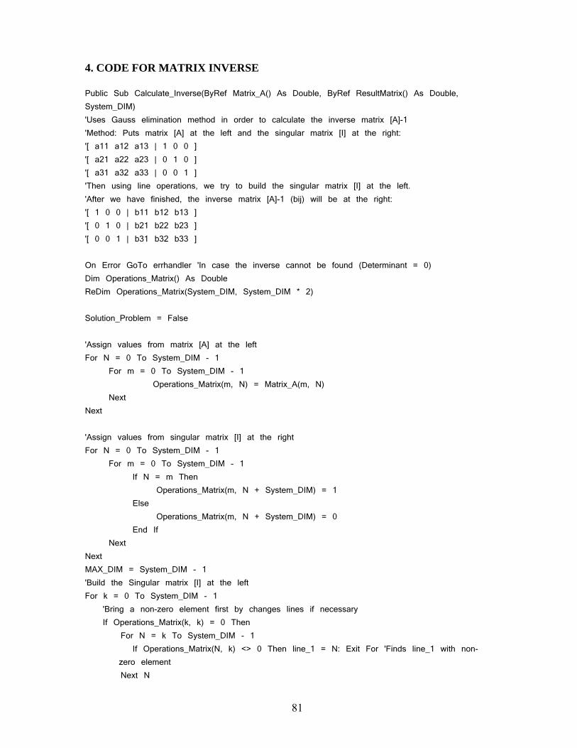
4. CODE FOR MATRIX INVERSE Public Sub Calculate_Inverse(ByRef Matrix_A() As Double, ByRef ResultMatrix() As Double, System_DIM) 'Uses Gauss elimination method in order to calculate the inverse matrix [A]-1 'Method: Puts matrix [A] at the left and the singular matrix [I] at the right: '[ a11 a12 a13 | 1 0 0 ] '[ a21 a22 a23 | 0 1 0 ] '[ a31 a32 a33 | 0 0 1 ] 'Then using line operations, we try to build the singular matrix [I] at the left. 'After we have finished, the inverse matrix [A]-1 (bij) will be at the right: '[ 1 0 0 | b11 b12 b13 ] '[ 0 1 0 | b21 b22 b23 ] '[ 0 0 1 | b31 b32 b33 ] On Error GoTo errhandler 'In case the inverse cannot be found (Determinant = 0) Dim Operations_Matrix() As Double ReDim Operations_Matrix(System_DIM, System_DIM * 2) Solution_Problem = False 'Assign values from matrix [A] at the left For N = 0 To System_DIM - 1 For m = 0 To System_DIM - 1 Operations_Matrix(m, N) = Matrix_A(m, N) Next Next 'Assign values from singular matrix [I] at the right For N = 0 To System_DIM - 1 For m = 0 To System_DIM - 1 If N = m Then Operations_Matrix(m, N + System_DIM) = 1 Else Operations_Matrix(m, N + System_DIM) = 0 End If Next Next MAX_DIM = System_DIM - 1 'Build the Singular matrix [I] at the left For k = 0 To System_DIM - 1 'Bring a non-zero element first by changes lines if necessary If Operations_Matrix(k, k) = 0 Then For N = k To System_DIM - 1 If Operations_Matrix(N, k) <> 0 Then line_1 = N: Exit For 'Finds line_1 with non-

zero element Next N

81

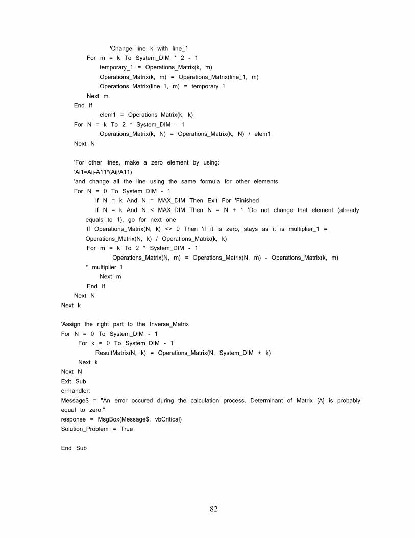
'Change line k with line_1 For m = k To System_DIM * 2 - 1 temporary_1 = Operations_Matrix(k, m) Operations_Matrix(k, m) = Operations_Matrix(line_1, m) Operations_Matrix(line_1, m) = temporary_1 Next m End If elem1 = Operations_Matrix(k, k) For N = k To 2 * System_DIM - 1 Operations_Matrix(k, N) = Operations_Matrix(k, N) / elem1 Next N 'For other lines, make a zero element by using: 'Ai1=Aij-A11*(Aij/A11) 'and change all the line using the same formula for other elements For N = 0 To System_DIM - 1 If N = k And N = MAX_DIM Then Exit For 'Finished If N = k And N < MAX_DIM Then N = N + 1 'Do not change that element (already

equals to 1), go for next one If Operations_Matrix(N, k) <> 0 Then 'if it is zero, stays as it is multiplier_1 =

Operations_Matrix(N, k) / Operations_Matrix(k, k) For m = k To 2 * System_DIM - 1 Operations_Matrix(N, m) = Operations_Matrix(N, m) - Operations_Matrix(k, m)

* multiplier_1 Next m End If Next N Next k 'Assign the right part to the Inverse_Matrix For N = 0 To System_DIM - 1 For k = 0 To System_DIM - 1 ResultMatrix(N, k) = Operations_Matrix(N, System_DIM + k) Next k Next N Exit Sub errhandler: Message$ = "An error occured during the calculation process. Determinant of Matrix [A] is probably equal to zero." response = MsgBox(Message$, vbCritical) Solution_Problem = True End Sub

82

5. CODE FOR ‘h’ IN HORIZONTAL PLATES Sub Computehlower() If Worksheets("input").Range("n6") = "" Or Worksheets("input").Range("n8") = "" Or

Worksheets("input").Range("n10") = "" Or Worksheets("input").Range("n12") = "" Then MsgBox ("Plz. Enter the Input Parameters") Exit Sub

End If If Worksheets("input").Range("n6") - Worksheets("input").Range("n8") > 0 Then

MsgBox ("Plz Check temparatures: ----- Air Temp. Exceeds Body Temp.") Exit Sub

End If Call xxx(ra, k, l) If ra < 10 ^ 7 Then

nu = 0.54 * ra ^ 0.25 Else

If ra >= 10 ^ 7 And ra < 3 * 10 ^ 10 Then nu = 0.15 * ra ^ 0.333 Else MsgBox ("Rayleigh Number is Greater Than 3*10^10 ..check out Input Parameters.")

End If End If

hlower = nu * k / l Worksheets("input").Range("n14") = hlower

End Sub Sub Computehupper() If Worksheets("input").Range("n6") = "" Or Worksheets("input").Range("n8") = "" Or




End If Call xxx(ra, k, l)

If ra < 3 * 10 ^ 10 Then nu = 0.27 * ra ^ 0.25 Else MsgBox ("Rayleigh Number is Greater Than 3*10^10..Plz. Check Out

Input Parameters.") End If

hupper = nu * k / l Worksheets("input").Range("n16") = hupper

End Sub Sub Clearhhorizontal()

83

Worksheets("input").Range("n6:n16") = "" End Sub Public Function xxx(ra, k, l)

l = Worksheets("input").Range("n10") * Worksheets("input").Range("n12") / 2 * (Worksheets("input").Range("n10") + Worksheets("input").Range("n12")) t = (Worksheets("input").Range("n6") + Worksheets("input").Range("n8")) / 2 tf = t + 273 beta = 1 / tf g = 9.81 cp = 1030.5 - 0.19975 * tf + 0.00039734 * tf ^ 2 + 0.000000083504 * tf ^ 3 rho = 351.99 / tf + 344.84 / tf ^ 2 mu = 0.000001492 * tf ^ 1.5 / (109.1 + tf) k = 0.002334 * tf ^ 1.5 / (164.54 * tf) * 100 v = mu / rho pr = mu * cp / k gr = g * beta * (Worksheets("input").Range("n8") - Worksheets("input").Range("n6")) * l ^ 3 / v ^ 2 ra = pr * gr

End Function 6. CODE FOR CLEARING SHEETS Sub clearinputsheet()

Worksheets("input").Range("d8:d12") = "" Worksheets("input").Range("i9:i15") = "" Worksheets("input").Range("n6:n16") = "" Worksheets("input").Range("c26:o117") = ""

End Sub Sub clearjointssheet()

Worksheets("joints").Range("c16:j40") = "" End Sub Sub clearnodessheet()

Worksheets("nodes").Range("b7:h1000") = "" End Sub Sub clearnetworksheet()

Worksheets("network").Range("c6:d600") = "" End Sub Sub clearallsheets()

YesNo = MsgBox("This will Delete Data in all The Sheets .. Do you want to Continue?", vbYesNo + vbCritical, "Caution") Select Case YesNo Case vbNo

Exit Sub Case vbYes

Call clearinputsheet Call clearjointssheet

84

Call clearnodessheet Call clearnetworksheet Worksheets("output").Range("b6:d600") = ""

End Select End Sub 7. CODE FOR USER FORM IN JOINTS INPUT SHEET Private Sub CmdAddRow_Click() If cmbMaterial1.Text = "" Then

MsgBox ("Select Material 1") Exit Sub

ElseIf cmbMaterial2.Text = "" Then MsgBox ("Select Material 2") Exit Sub

ElseIf TxtForce = "" Then MsgBox ("Enter The Contact Force") Exit Sub

ElseIf TxtFCurrent = "" Then MsgBox ("Enter The Fraction of Total Current") Exit Sub

End If

Dim i Dim j Dim Row1 Dim Q Dim Cth Dim F Dim S Dim s1 Dim s2 Dim k Dim X Dim Counter

i = cmbMaterial1.ListIndex + 8 j = cmbMaterial2.ListIndex + 8 s1 = Worksheets("Data").Cells(i, 4) s2 = Worksheets("Data").Cells(j, 4) Row1 = (Worksheets("Data").Cells(i, 5) + Worksheets("Data").Cells(j, 5)) k = (Worksheets("data").Cells(i, 7) + Worksheets("data").Cells(j, 7)) / 2 F = TxtForce / 9.81 * 1000

If s1 < s2 Then S = s1

Else S = s2

85

End If X = (Row1 / 2.506628275) * (S / F) ^ 0.5 * 1000 * 10 ^ -6 Row1 = Row1 / 2 i = TxtFCurrent * Worksheets("Input").Cells(8, 4)

Q = i ^ 2 * X Cth = 2.1 * Row1 * k / X * 10 ^ -6

Counter = 16 While (Worksheets("Joints").Cells(Counter, 5)) <> ""

Counter = Counter + 1 Wend

Worksheets("Joints").Cells(Counter, 4).Interior.Color = 8421376 Worksheets("Joints").Cells(Counter, 5).Interior.Color = 8421376 Worksheets("Joints").Cells(Counter, 6).Interior.Color = 8421376 Worksheets("Joints").Cells(Counter, 7).Interior.Color = 10092500 Worksheets("Joints").Cells(Counter, 8).Interior.Color = 10092543 Worksheets("Joints").Cells(Counter, 9).Interior.Color = 10092543 Worksheets("Joints").Cells(Counter, 10).Interior.Color = 10092543 Worksheets("Joints").Cells(Counter, 3).Interior.Color = 8421376 'Worksheets("Joints").Cells(Counter, 3).Border = xlAll Worksheets("Joints").Cells(Counter, 3).Font.Color = 10092543 Worksheets("Joints").Cells(Counter, 4).Font.Color = 10092543 Worksheets("Joints").Cells(Counter, 5).Font.Color = 10092543 Worksheets("Joints").Cells(Counter, 6).Font.Color = 10092543 Worksheets("Joints").Cells(Counter, 3) = TxtJName Worksheets("Joints").Cells(Counter, 4) = TxtJType Worksheets("Joints").Cells(Counter, 5) = F * 9.81 / 1000 Worksheets("Joints").Cells(Counter, 6) = Val(TxtFCurrent) Worksheets("Joints").Cells(Counter, 7) = i Worksheets("Joints").Cells(Counter, 8) = X Worksheets("Joints").Cells(Counter, 9) = Cth Worksheets("Joints").Cells(Counter, 10) = Q

End Sub Private Sub CommandButton1_Click()

Unload Me End Sub Private Sub UserForm_Initialize()

i = 8 While (Worksheets("Data").Cells(i, 3)) <> "" cmbMaterial1.AddItem Worksheets("Data").Cells(i, 3)

cmbMaterial2.AddItem Worksheets("Data").Cells(i, 3) i = i + 1

Wend End Sub

86

8. CODE FOR USER FORM IN NODES SHEET Private Sub CmdAir_Click() If LTrim(RTrim(Me.TxtAirTEmp)) = "" Then

MsgBox "Enter Air Temparature" ElseIf LTrim(RTrim(Me.TxtTempZone)) = "" Then

MsgBox "Enter Air zone" Else

i = 7 While (Worksheets("nodes").Cells(i, 2)) <> ""

i = i + 1 Wend

Worksheets("nodes").Cells(i, 2) = i - 6 Worksheets("nodes").Cells(i, 3) = Me.TxtTempZone Worksheets("nodes").Cells(i, 4) = 2 Worksheets("nodes").Cells(i, 8) = Me.TxtAirTEmp Worksheets("nodes").Cells(i, 7).Select

End If End Sub Private Sub cmdComponent_Click()

Dim i Dim j Dim k Dim z j = 26 + CmbComponent.ListIndex i = 7

While (Worksheets("nodes").Cells(i, 2)) <> "" i = i + 1

Wend z = Worksheets("input").Cells(j, 4) For k = 1 To z

Worksheets("nodes").Cells(i, 2) = i - 6 Worksheets("nodes").Cells(i, 3) = Worksheets("input").Cells(j, 3) Worksheets("nodes").Cells(i, 4) = 1 Worksheets("nodes").Cells(i, 6) = Worksheets("input").Cells(j, 15) Worksheets("nodes").Cells(i, 5) = Worksheets("input").Cells(j, 14) Worksheets("nodes").Cells(i, 7) = Worksheets("input").Cells(j, 13) Worksheets("nodes").Cells(i, 7).Select i = i + 1

Next End Sub Private Sub CmdDummy_Click()

Dim i Dim j

87

Dim k Dim z i = 7


Wend Worksheets("nodes").Cells(i, 2) = i - 6 Worksheets("nodes").Cells(i, 3) = "Dummy Node" Worksheets("nodes").Cells(i, 4) = 1 Worksheets("nodes").Cells(i, 6) = 0 Worksheets("nodes").Cells(i, 5) = 0 Worksheets("nodes").Cells(i, 7) = 0 Worksheets("nodes").Cells(i, 7).Select

End Sub Private Sub CmdJoint_Click()

Dim i Dim j Dim k Dim z j = 16 + cmbjoint.ListIndex i = 7


Wend Worksheets("nodes").Cells(i, 2) = i - 6 Worksheets("nodes").Cells(i, 3) = Worksheets("Joints").Cells(j, 3) Worksheets("nodes").Cells(i, 4) = 1 Worksheets("nodes").Cells(i, 6) = 0 Worksheets("nodes").Cells(i, 5) = Worksheets("Joints").Cells(j, 9) Worksheets("nodes").Cells(i, 7) = Worksheets("joints").Cells(j, 10) Worksheets("nodes").Cells(i, 7).Select

End Sub Private Sub OptionButton1_Click()

FrComp.Enabled = True Frame1.Enabled = False CmdDummy.Enabled = False FrAir.Enabled = False


FrComp.Enabled = False Frame1.Enabled = True CmdDummy.Enabled = False FrAir.Enabled = False

End Sub

88

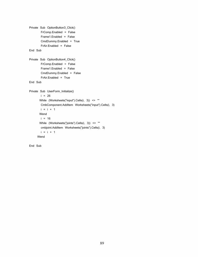
Private Sub OptionButton3_Click()

FrComp.Enabled = False Frame1.Enabled = False CmdDummy.Enabled = True FrAir.Enabled = False


FrComp.Enabled = False Frame1.Enabled = False CmdDummy.Enabled = False FrAir.Enabled = True

End Sub Private Sub UserForm_Initialize()


CmbComponent.AddItem Worksheets("input").Cells(i, 3) i = i + 1

Wend i = 16

While (Worksheets("joints").Cells(i, 3)) <> "" cmbjoint.AddItem Worksheets("joints").Cells(i, 3) i = i + 1

Wend End Sub

89

ACKNOWLEDGEMENT

Successful completion of work will never be one man’s task. It requires hard work in right

direction. There are many who have helped to make my experience as a student a rewarding

one.

In particular, I express my gratitude and deep regards to my thesis guide Dr. Dayal R. Parhi

first for his valuable guidance, constant encouragement & kind co-operation throughout

period of work which has been instrumental in the success of thesis.

I also express my gratitude & regards to Deepak Raorane (COE, GE, IIC, Hyderabad),

company guide Debabrata Mukherjee and Sudhakar Pachunoori for their scientific advice

and eagerness to help during my work at GE, IIC, Hyderabad

I also express my sincere gratitude to Dr. B. K. Nanda, Head of the Department, Mechanical

Engineering, for providing valuable departmental facilities.

I would like to thank Prof. N. Kavi, P.G Coordinator, Mechanical Engineering Department

and Prof. K.R.Patel, Faculty Adviser.

I thank my friend, Jaydev Sirimamilla who helped me and turned the task of learning

software required for the project a joy.

I would like to thank my fellow post-graduate students, Tulasi Ram, SadikaBaba, Rajesh and

Sundeep who made learning science a joy.

Krishna Swamy Cherukuri

i

TABLE OF CONTENTS CHAPTER Page No

Acknowledgement i

Abstract v

List of Figures vi

List of Tables viii

1. INTRODUCTION 1-2

1.1 Background 1

1.2 Objective 1

2. LITERATURE SURVEY 3-6


2.2 Contact resistance 3

2.2.1 Electrical Contact Resistance 4

2.2.2 Thermal Contact Resistance 5

3. INTRODUCTION TO SWITCH GEAR 7-13

3.1 Introduction 7

3.2 Switch Gear 7

3.3 Circuit Breaker 9

3.4 Current Flow Path in a Switch Gear 11

4. THERMAL NETWORK THEORY 14-35

4.1 Introduction 14

4.2 Electrical and Thermal Analogy 15


4.4 The Lumped-parameter Method for Steady State Solution 17

4.5 The Lumped-Parameter Method for Transient Solution 18

4.6 Building Thermal Network 18

4.7 Nodes 19

4.8 Conductors 20

4.9 Criteria for Selecting Nodes 21

4.10 Node Equations 22

ii

4.11 Node Equation at Joint 28

4.12 Convection 32

4.12.1 Convective Heat Transfer Co-efficient 32

4.12(a) h Correlations for Vertical Plate in Natural Convection 33

4.12(b) h Correlations for Horizontal Plate in Natural Convection 34

4.1.3 Effect of Radiation 35

5. JOINT RESISTANCE 36-47

5.1 Types of Joints 36

5.2 Types of Electrical Contacts 37

5.3 Electrical Contact Resistance 39

5.4 Calculation of Electrical Contact Resistance 40

5.2.1 Maxwell’s Formula 40

5.2.2 Greenwood’s Formula 40

5.2.3 Empirical Relations 41

5.5 Thermal Contact Resistance 43

5.5.1 Relation Based on Thermo-Electromechanical Properties 47

6. PROBLEM SOLVING PREOCESS 48-67

6.1 Problem Definition 48

6.2 Steps in Solving the Problem 48

6.2.1 Electrical Network Diagram 49

6.2.2 Electrical Resistance Calculation 53

6.2.3 Comparison with Measured Value 54

6.2.4 Thermal Network Diagram 54

6.2.5 Calculation of Input Parameters 59

6.2.6 Convective Heat Transfer Co-efficient Calculation 59

6.3 Analytical Tool to Calculate Temperatures 59

6.3.1 Input Sheet 60

6.3.2 Joints sheet 62

6.3.3 Nodes Sheet 64

6.3.4 Network Sheet 66

6.3.5 Output Sheet 67

iii

7. RESULTS 68-80

7.1 Frame 3 68

7.1.1 Reasons for Temperature Deviation 69

7.1.2 Regions of Maximum Deviation 70

7.1.3 Results Comparison 70

7.1.3(a) Phase A 70

7.1.3(b) Phase B 72

7.1.3(c) Phase C 74

7.1.4 Temperature Prediction 75

7.1.4(a) Change in Run –In Geometry 75

7.1.4(b) Change in Heat Sink Surface Area 76

7.1.4(c) Increasing Cluster Contact Force 78

7.2 FRAME 1 79

8. CONCLUSION AND FURTHER WORK 81-82

8.1 Contribution 81

8.2 Conclusion 81

8.3 Further Work 82

9. REFERENCES 83-85

APPENDIX-A

Visual Basic Code used in Analytical Tool 86-98

iv

ABSTRACT



equipments for safe operation. So during the design phase of any electrical equipment

thermal analysis is mandatory to predict the temperature rise.






The problem is considered as two parts. As first part, an Excel tool is developed with

Visual Basic backend, based on thermal networking method to calculate steady state

temperatures in electrical equipments. Here the numerical method used is Elementary

Balance Method, in which every element is represented by a node and relevant energy

balance equations are formulated for it. Temperatures are calculated using the Excel tool for

frame 1 and 3. Test (Thermal Run) is conducted on AKD-12 switch gear (frame 1 and frame

3) under continuous current to find out temperatures. Analytical results from the tool are then

validated against the test data.




Good matching is observed in temperature profile between analytical and

experimental results. The maximum percentage error is 15%.By analyzing the results, it can

be concluded that thermal network theory helps engineers to predict temperatures easily for

changes in design reducing design cycle time and it is flexible as to expand its application to

any heat generating equipment.

v

LIST OF FIGURES

Page No

Figure 3.1 GE Switch Gears Figure 8

Figure 3.2 MCB 10

Figure 3.3 Powervac MV Vacuum Distribution Breaker 10

Figure 3.4 115,000 V Breaker at Generating Station 10

Figure 3.5 1250 A air circuit Breaker 10

Figure 3.6 Switch Gear Line Diagram 11

Figure 3.7 Switch Gear Line Diagram showing Joints 12

Figure 4.1 Network Representation 23

Figure 4.2 Heat Balance at a Node 23

Figure 4.3 Energy Balance at Node 2 26

Figure 4.4 Network Representation at a joint 28

Figure 5.1 Effect of Contact Pressure on Contact Resistance 40

Figure 5.2 Set of Circular Contact Spots showing the Symbol Notation 41

Figure 5.3 – Constriction of Heat Flow through an Interface formed by two Materials. 43

Figure 5.4 Temperature drop on either side of interface 44

Figure 5.5 Heat transfer paths at an interface 45

Figure 5.6 Thermal Resistance Network for nonconforming rough contacts 45

Figure 5.7 Thermal contact problem. 46



Figure 6.3 Electrical Network Diagram for frame 3 with3 phases 52



Figure 6.6 Thermal Network Diagram for Cluster Pad region 57

Figure 6.7 Input Sheet 61

Figure 6.8 Input Form for Joints 62

Figure 6.9 Joints Sheet 63

vi

Figure 6.10 Input Form for Nodes 64

Figure 6.11 Nodes Sheet 65

Figure 6.12 Network Sheet 66

Figure 6.13 Output Sheet 67

Figure 7.1 Frame 3 Temperature profile 68

Figure 7.2 Temperatures comparison for Phase A 72


Figure 7.4 Temperatures comparison for Phase B 73


Figure 7.6 Temperatures comparison for Phase C 74


Figure 7.8 Temperature Profile with change in Run-in Geometry 76

Figure7.9 Temperature variation by doubling Surface Area 77

Figure7.10 Temperature variation for change in Cluster Contact Force 78

Figure7.11 Frame -1 Temperature Profile 80

vii

LIST OF TABLES

Page No

Table 3.1 Electrical and Thermal Analogy 15

Table 5.1 K Factor Values 43

Table 5.2 – Thermal Contact Conductance Models 46

Table 7.1 Temperatures at Different Point in Frame3 69

Table 7.2 Temperatures on Phase A 71

Table 7.3 Run-In Geometry 75

Table 7.4Analytical Temperatures with and without change in Run-In Dimensions 75

Table 7.5 Analytical Temperatures Comparison by doubling the Heat Sink Surface Area 77

Table 7.6 Analytical Temperatures Comparison by increasing Contact Force at clusters 78

Table 7.7 Temperatures for Frame1 79

viii

1. INTRODUCTION

This chapter gives an overview of the project work reported in the thesis. First,

background of the project work is outlined followed by the objective and methodology

followed to achieve the objective.

1.1 BACKGROUND



equipments for safe operation. So during the design phase of any thermal equipment thermal

analysis is mandatory to predict the temperature rise. Bypassing thermal analysis precludes

design optimization.

Thermal analysis is done either by building a laboratory model or by simulation using

simulation softwares. Generally once the basic design is completed, laboratory model is built

to observe the response of the system. Later certain changes are incorporated to arrive at

optimum design. Rebuilding the model for every change incorporated becomes a costly affair.

So simulation work is carried out at this stage using simulation software to predict the

response of the system for the changes made.

By this, though cost involved in rebuilding the lab model is cut down, time required

in predicting the response of the system for new design or changes cannot be avoided. This is

so because, in simulation software rebuilding the model, meshing, changing the boundary

conditions and running the solution for any change in geometry of the components involves

considerable time. So, one is interested to predict temperature variations in very less time

using simple mathematical calculations even at the sacrifice of accuracy to certain extent.

1.2 OBJECTIVE




1



Following methodology is followed to achieve the objective. The problem is

considered as two parts. As first part, an Excel tool is developed with Visual Basic backend,

based on thermal networking method to calculate steady state temperatures in electrical

equipments. Here the numerical method used is Elementary Balance Method, in which every

element is represented by a node and relevant energy balance equations are formulated for it.


for frame 1 and 3. Test (Thermal Run) is conducted on AKD-12 switchgear, frame 1 and

frame 3 under continuous current to find out temperatures at different points along the

current flow path. Analytical results from the tool are then validated against the test data.

Good matching is observed in temperature profile between analytical and experimental

results.




2

2. LITERATURE SURVEY

This chapter surveys the literature in the areas of thermal network modeling, electrical

contact resistance and thermal contact resistance.

2.1THERMAL NETWORK THEORY

Peter and Hans [1] have carried out thermal simulation of a circuit Breaker to find out steady

state temperatures considering all modes of heat transfer. The analysis is done based on

software developed using thermal networking with a capacity of 32000 nodes. The paper

explains the thermo- Electrical coupling to represent electrical carrying conductor by thermal

components.

Correspondence from IEEE [2] describes a relatively simple method for manual thermal

computations, particularly useful for electronic equipment where all types of heat transfer

must be taken into account. The method involves construction of a simplified thermal

network diagram for the equipment. The method of thermal computation described here

exploits the similarity between thermal and electrical analogy, shown in table [4.1].

Hiroshi and Kazunori [3] have described the way to develop thermal network diagram for

low voltage circuit breaker.

Hefner and Blackburn published a paper [9] giving thermal Component simulation for

electro-thermal network simulation. It explains the structure of the electro-thermal

semiconductor device models indicating the interaction with the thermal and electrical

networks through the electrical and thermal terminals, respectively.

2.2 CONTACT RESISTANCE

An accurate knowledge of contact mechanics, that is, the pressure distribution, the size of

contact area, and the mean separation between surface planes as functions of applied load,

and the geometrical and mechanical characteristics/properties of the contacting bodies, plays

an important role in predicting and analyzing thermal and electrical contact resistance and

many tribological phenomena.[6]

3

2.2.1 Electrical Contact Resistance

The calculation of the contact resistance between two rough electrodes is a difficult task,

since the contact interface comprises many spots corresponding to more or less conducting

paths for the electrons [4].

In 1966, J. A. Greenwood published a paper entitled [12] in which the author derived a

formula [5.2] for the constriction resistance of a set of circular spots [Fig.5.2], with each spot

located at the end of a metallic electrode. The electrodes communicate via the spots with no

interface film between them. In the same paper author presented a formula resulting from an

approximation which holds when there is no correlation between the size of a given spot and

its position.

For some ten years now, contact resistance has been computed numerically mainly by

Nakamura and Minowa [13], who use the finite element method (FEM) and the boundary

element method (BEM) from a different point of view, considering a system of two cubic

electrodes communicating through square spots.

Finally, it should also be mentioned that a recent paper by R. S. Timsit reviews the

dependence of electrical resistance on the shape and dimensions of the contact spots [14].

Maxwell’s formulation for single contact spot is given by formula [5.1]. With increase in

contact pressure, the electrical contact resistance decreases at the joint as shown in graph

[4.1].

In the paper published by Peter and Hans [1], electrical contact resistance is given in terms of

contact force, contact material type and shape of the contact, shown by formula [5.3]. Based

on these formulae, empirical relations [5.4, 5.5] are developed which can be used for bolted

and spring loaded contacts for different materials. Those empirical relations are used here to

calculate the electrical contact resistance.

4

2.2.2 Thermal Contact Resistance

Heat transfer across interfaces formed by mechanical contact of nonconforming rough solids

occurs in a wide range of applications, such as microelectronics cooling, spacecraft structures,

satellite bolted joints, nuclear engineering, ball bearings, and heat exchangers. Because of

roughness of the contacting surfaces, real contacts in the form of micro contacts occur only at

the top of surface asperities, which are a small portion of the nominal contact area, normally

less than a few percent. As a result of curvature or out-of flatness of the contacting bodies, a

macro contact area is formed, the area where the micro contacts are distributed.

Two sets of resistances in series can be used to represent the thermal contact resistance (TCR)

for a joint, the large scale or macroscopic constriction resistance RL and the small-scale or

microscopic constriction resistance Rs as shown in formula [5.7].

Cooper et al. [15] studied the contact conductance of rough, conforming metals experiencing

light to moderate pressure. The model presumes that the micro contacts deform plastically.

Mikic [16] developed models for the macroscopic and microscopic contact conductance that

took into account non-uniform pressure distributions, but did not specify how the

distributions were determined. The microscopic conductance model uses the plastic

deformation model of Cooper, et al. (1969).

Thomas and Sayles [17] studied the relative effects of waviness and roughness on thermal

contact conductance. They observe that the total roughness of a specimen is related to its size,

defining a dimensionless waviness number.

Yovanovich [18] refined the model of Cooper, et al. (1969) for plastic deformation of

microscopic contacts on conforming surfaces.

Lambert [19] and Lambert and Fletcher [20] developed a model for the thermal contact

conductance of spherical rough metals that is valid in regions removed from the limiting

cases of rough/flat, smooth/spherical surfaces. It is, however, a single macro contact model,

and requires loading on the macrocontact as well as the surface geometry of the contact. In

5

multiple macrocontact situations, such as those encountered in large area contacts, it is

difficult to estimate number of macrocontact, much less the loading on each macrocontact.

Table 5.1 lists the dimensional and non-dimensional contact conductance correlations

reviewed in this section.

Peter and Hans published a paper in which the thermal contact resistances are deduced from

the electrical contact resistances. [1] The formulae used [5.8] here for thermal contact

resistance calculations are based on this paper. The thermal conductivity of the contacts is

increased by a factor of 2.1 to account for the thermal conductivity of the air in the voids of

the contact area.

6

3. INTRODUCTION TO SWITCHGEAR

3.1 INTRODUCTION

Circuit protection devices are needed to protect personnel and circuits from hazardous

conditions. The hazardous conditions can be caused by a direct short, excessive current or

excessive heat. Circuit protection devices are always connected in series with the circuit

being protected.

Every one is familiar with low voltage switches and rewire-able fuses. A switch is

used for opening and closing an electric circuit and a fuse is used for over current protection.

Every electric circuit needs a switching device (Switch) and a protective device (Fuse). The

switching and protective devices have been developed in various forms depending voltage

and current. Switchgear is a general term covering a wide range of equipment concerned with

switching and protection.

3.2 SWITCHGEAR

The term switchgear, commonly used in association with the electric power system,

or grid, refers to the combination of electrical disconnects and/or circuit breakers used to

isolate electrical equipment. All equipments associated with the fault clearing process are

covered by the term “Switchgear”. Switchgear is an essential part of power system and also

that of any electric circuit. Between the generating station and final load point, there are

several voltage levels and fault levels. Hence, in various applications, the requirements of

switchgear vary depending upon the location, ratings and switching duty. Switchgear

includes switches, fuses, circuit breakers, isolators, relays, control panels, lightening arresters,

current transformers and various associated equipments.

3.2.1Protective Relay: The protective relays are the automatic devices, which can sense the

fault and send instructions to the associated circuit breaker to open.

3.2.2Circuit Breakers: Circuit breakers are the switching and current interrupting devices.

Basically a circuit breaker comprises a set of fixed and movable contacts. The contacts can

be separated by means of an operating mechanism. The separation of the current carrying

7

contacts produces an arc. The arc is extinguished by a suitable medium like dielectric oil, air,

vacuum and SF6 gas.

3.2.3 Isolators: Isolators are disconnecting switches, which can be used for disconnecting a

circuit under no current condition. They are generally installed along with circuit breaker. An

isolator can be opened after the circuit breaker. After opening the isolator the earthing switch

can be closed to discharge the charges to the ground.

3.2.4 Transformers: The current transformers and the potential transformers are used for

transforming the current and voltage to a lower value for the purpose of measurement,

protection and control.

3.2.5 Lightening Arresters: Lightening arresters (surge arresters) divert the over-voltages

to earth and protect the sub-station equipment from over voltages.

Some of GE Switchgear products:

Figure 3.1 GE Switchgears A - AKD 10 Low Voltage Metal Enclosed

B - Paralleling switch Gear

C - Entellisys Low Voltage switch Gear

D - Power/Vac® Medium Voltage Metal Clad Switch Gear

8

3.3 CIRCUIT BREAKER

A circuit breaker is an automatically-operated electrical switch designed to protect an

electrical circuit from damage caused by overload or short circuit. It is a device to open or

close an electric power circuit either during normal power system operation or during

abnormal conditions. During abnormal conditions, when excessive current develops, a circuit

breaker opens to protect equipment and surroundings from possible damage due to excess

current. These abnormal currents are usually the result of short circuits created by lightning,

accidents, deterioration of equipment, or sustained overloads. Unlike a fuse, which operates

once and then has to be replaced, a circuit breaker can be reset (either manually or

automatically) to resume normal operation. Circuit breakers are made in varying sizes, from

small devices that protect an individual household appliance up to large switchgear designed

to protect high voltage circuits feeding an entire city. Based on voltage, switch gears are

classified as

3.3.1 Low voltage Circuit Breakers

Low voltage circuit breakers have voltage ratings from 250 to 600 V AC and 250 to 700 V

DC. They are two types.

MCB-(Miniature Circuit Breaker Rated current is not more than 100 A.

MCCB-(Molded Case Circuit Breaker) Rated current is up to 1000 A.

Figure 3.2 MCB Figure 3.3 PowerVac - MV Vacuum Distribution Breaker

rated up to 72.5 kV

3.3.2 Medium Voltage Breakers

Medium voltage circuit breakers are

9

3.3.3 High-Voltage Breakers

nely available up to 765 kV AC. They are broadly classified

3. Air blast

High voltage breakers are routi

by the medium used to extinguish the arc as:

1. Oil-filled (dead tank and live tank)

2. Oil-filled (minimum oil volume) 4. Sulfur hexafluoride

Figure 3.4 1200 A, 3-pole 115,000 V Figure 3.5 Front panel of a 1250 A air

Small circuit breakers are either installed directly in equipment, or are arranged in a

breaker

3.4 CURRENT FLOW PATH IN SWITCHGEAR

Current flow path in switchgear involves many components of different cross sections

joined

Breaker at a generating station circuit breaker manufactured by ABB

panel. Power circuit breakers are built into switchgear cabinets. High-voltage

breakers may be free-standing outdoor equipment or a component of a gas-insulated

switchgear line-up

with different types of joints and contacts. Generally joints involved are bolted joints

and spring contacts. The components in the current flow path are test links, power connects,

lower vertical busbars, run-ins, cluster fingers, cluster pad, line terminal, flexible conductors,

moving conductors, load terminal, runbacks, upper vertical busbars and outgoing horizontal

busbars. Figure 3.6 shows line diagram of current flow path for switchgear. Current enters

the switchgear through test link which is connected to power source. Current then flows to

10

http://www.answers.com/topic/circuit-breaker-115-kv-jpg

http://www.answers.com/topic/largecircuitbreaker-jpg

lower vertical busbar thorough power connect. Power connect is a clamp like device used for

joining horizontal test links to vertical busbars.

Figure3.6 Switchgear Line Diagram

A busbar in electrical power distribution refers to thick strips of copper or aluminum

that conduct electricity within a switchboard, distribution board, substation or other electrical

apparatus. From busbar, current flow to circuit breaker through run-in, cluster fingers and

cluster pad. Run-ins are horizontal strips that connect gear with circuit breaker electrically.

Cluster fingers are spring loaded thin strips connecting run-ins with cluster pad. Components

in a circuit breaker are line terminal, flexible conductors, moving conductors and load

terminal. Current from circuit breaker flows through runbacks to upper vertical busbars.

From vertical busbars, current leaves the switch gear through power connect and horizontal

busbars.

11

Figure3.7 Switchgear line Diagram Showing Joints

Figure 3.7 shows joints between different components in the switchgear. Joints at

cluster fingers and moving contact are spring loaded contacts. All the remaining joints are

bolted joints with bolts of different sizes and numbers depending upon the clamping force

required at the joint. Except the test links and horizontal busbars, all the components are

placed inside a compartment as shown by dotted line. Compartment with busbars is called

busbar compartment and compartment with circuit breaker is called breaker compartment.

12

4. THERMAL NETWORK THEORY

4.1 INTRODUCTION

During the design of electrical and electronic equipments, thermal analysis of the

system is very essential and disregard of a thermal analysis may lead to inadequate thermal

design. Sometimes schedules and cost aspects exclude construction of thermal laboratory

models which many a times lands up in severe financial penalties. In some instances such

analysis is bypassed because of its complexity. This bypassing precludes design optimization.

Thermal deficiencies in performance of the equipment may then result.

So conducting thermal analysis for any electrical system is inevitable either by

building a laboratory model or by simulating the thermal analysis using simulation software.

Generally once the basic design is completed, laboratory model is built to observe the

response of the system. Later certain changes are incorporated to arrive at optimum design.

Rebuilding the model for every change incorporated becomes a costly affair. So simulation

work is carried out at this stage using simulation software to predict the response of the

system for the changes made.

Thermal simulation can be carried out using many types of software like ANSYS,

CFD, FLUX etc and results can be predicted very precisely. By this, though cost involved in

rebuilding the lab model is cut down, time required in predicting the response of the system

for new design or changes cannot be avoided. This is so because, in simulation software

rebuilding the model, meshing, changing the boundary conditions and running the solution

for any change in geometry of the components involves considerable time. So one is

interested to have an analytical tool which can predict the results in lesser time even by

compromising with the accuracy of results up to some extent. This gave birth to a relatively

simple method for manual thermal computations, particularly useful for electronic and

electrical equipment where all types of heat transfer must be taken into account. The method

involves construction of a simplified thermal network diagram for the equipment, developing

energy equation at each node and solving for temperature rise. When good judgment is used,

predicted temperature values approach actual ones.

13

4.2 ELECTRICAL AND THERMAL ANALOGY

The method of thermal computation used here exploits the similarity between thermal

and electrical networks as shown in Table 4.1. Heat flow is represented in the electrical

analog scheme by current flow, temperature potential is represented by voltage potential and

a thermal resistor by an electrical resistor. For transient heat flow, the analogy also applies in

that heat stored and absorbed in a mass may be represented by an electrical current stored and

absorbed in a capacitor.

Table 4.1 Electrical and Thermal Analogy

ELECTRICAL THERMAL Current, I = dq/dt [Amps] Heat flow, q [Joules/sec]

Voltage, V [Volts] Temperature difference, T [°C]

Resistance,

R = L/A [Ohms]

Ohm's Law: I = V/R

Heat transfer resistance, R

Rconvection = 1/(h A), Rconduction = KA/L

q = T / R

Capacitance, C = A/d [Farads]

I = C dV/dt

Thermal heat capacity, m cp

q = m cp dT/dt

Time constant, T= R. C Time constant, Tth = Rth . W.CP

Ohm’s law for current flow

One dimensional steady flow equation

P = I V [Watts] P = T q [Watts °C]

Kirchhoff's Current Law

I = 0

Energy equation

q = 0

Charge, q = I dt [Coulombs] Heat, Q = q dt [Joules]

Kirchhoff's Voltage Law

V = 0

T = 0

14

Current flow through resistor, stored in

capacitor

Heat flow to ambient ,stored in mass of

material of specific heat cp

One dimensional current flow trough RC

network

One dimensional transient heat flow

through bar

4.3 THERMAL NETWORK THEORY

The finite difference method provides the basis for converting a distributed parameter

description of a system into a lumped parameter model of that system. We can expand the

concept of a finite node to include a larger macroscopic control volume (which physically

may be very large or small). In connecting individual control volumes, it is often useful to

use an electrical analogy to describe the system. In thermal systems, this electrical analogy

gives rise to the so-called thermal network model.

A thermal network is a representation (model) of the thermal characteristics of any

system modeled by considering points (nodes) at discrete parts of the system that are linked

by conductors through which heat may flow. This type of thermal network is often described

as a lumped parameter model because the thermal properties, such as the heat capacity, of a

part of the system are “lumped” together on the node representing that part.

The method developed here is called the Equivalent Thermal Network and takes

advantage of the theory of analogy between electrical and thermal elements. In steady state

temperature rise computations, current generators are used to represent heat generators, and

electrical resistances to represent the internal thermal conduction resistances. In transient heat

15

flow condition, capacitor is connected in parallel to represent the heat stored in the body

along with heat generator and thermal resistance. Here the mathematical model is based on a

numerical method called Elementary Balance Method, in which every element is represented

by a node and relevant energy balance equations are formulated for it.

4.4 THE LUMPED-PARAMETER METHOD FOR STEADY STATE SOLUTION

The lumped-parameter method involves dividing the object being analyzed into a

network of discrete nodes connected by thermal conductors. Each node is considered to be

isothermal i.e. has a single temperature associated with it.

To determine the steady state a heat balance is applied to each node,

Q 0=∑ (4.1)

Where Q represents heat input, and the removal of heat is regarded as a negative Q. The

symbol signifies a summation. In words, this can be stated: ∑

At any node, HEAT IN = HEAT OUT

Equation 4.1 is applied to each node in the model to obtain a system of simultaneous

equations from which all nodal temperatures are calculated.

4.5 THE LUMPED-PARAMETER METHOD FOR TRANSIENT SOLUTION

For evolution of temperatures in a model during the transient stage (not just the final

steady-state values) then the node equation acquires a time-derivative on the right-hand side.

The energy equation is written as dTQ m.cdt

=∑ (4.2)

Where, m is the mass of the node and C the specific heat capacity.

The derivative is approximated by finite differences (dT/dt).

Applying the above equation to all nodes, gives a system of algebraic equations that are

solved for temperature T at time t+dt. The solution is done by iterative method.

As the highest temperatures occur after the transient phase is over and the steady state

(thermal equilibrium) has been reached, we are interested to calculate the steady state

temperatures and so the entire work is concentrated on one dimensional steady state solution

16

by lumped parameter method. Most of the thermal calculations for electrical equipments are

limited to one dimensional only.

4.6 BUILDING THERMAL NETWORK

Building thermal network diagram for electrical equipment involves visualizing it as

thermal network with thermal resistances, heat generators and thermal capacitors. As the

work is limited to steady state, thermal capacitors are absent. First the entire structure is

descritized into number of nodes, each node representing a component with certain mass i.e.

a lumped mass. The nodes are taken as three types- diffusion nodes, boundary nodes and

arithmetic nodes. Each node is connected to the other by a conductor which represents

internal conduction resistance or convection resistance or radiation resistance. Conductors

are considered as two types—linear conductor and radiation conductors. Due to the current

flow in a element (node), there is some internal heat generation due to I2R loss and that

amount of heat is added as heat input at the corresponding node. With this the equipment is

represented as a network with different types of nodes with heat generation and connected by

different types of conductors.

4.7 NODES

At nodes energy is conserved. Each node has a single characteristic temperature ‘T’.

Nodes may represent the temperature of a finite volume of material. There are three types of

nodes, classified by their capacitance or ability to transiently store or release thermal energy.

4.7.1 Diffusion Nodes: Diffusion nodes have a finite capacitance ‘C’, usually equal to the

product of mass and specific heat (mCp or ρVCp). Diffusion nodes may represent a finite

volume and mass. These nodes are used in transient analysis.

4.7.2 Arithmetic Nodes: rithmetic nodes have zero capacitance. Energy flowing into an

arithmetic node must balance the energy flowing out at all times. These nodes are used in

steady state analysis as no heat is accumulated in the body once the system comes to

thermal equilibrium and all the heat in is equal to heat out. Heat source is added to these

nodes.

17

4.7.3 Boundary Nodes: Boundary nodes have an infinite capacitance, and hence usually

represent sources or sinks, large masses, or ideally controlled temperature zones. Air is

represented using these nodes.

4.8 CONDUCTORS

Conductors describe the means by which heat flows from one node to another. Each

conductor has a single characteristic conductance “G” (inverse of resistance). Conductors

represent energy paths via solid conduction, contact conduction, convection, advection,

radiation, etc. There are two types of conductors.

4.8.1 Linear Conductors: Linear conductors transport heat in direct proportion to the

difference in nodal temperatures

(4.3) 1 2 1 2Q G(T T− = − )

Q1-2 is the heat flow from node 1 to node 2 through a conductor of conductance G



Usually, linear conductors represent solid conduction with ‘G’, calculated as the product of

the material conductivity and inter nodal cross-sectional area, divided by the distance

between node centers.

KAGL

= (4.4)

Linear conductors may also represent convection conductance with ‘G’, calculated as the

product of convective heat transfer coefficient ‘h’ and surface area ‘a’. Here we represent

convective conductance by H to avoid confusion.

(4.5) H = h*a

4.8.2 Radiation Conductors: Radiation conductors transport heat according to the

difference in the fourth power of absolute temperature.

(4.6) 4 41 2 1 2Q G(T T− = − )

They are used almost exclusively for radiation heat transfer, with

18

1 1 2 1G F− A= σε (4.7)

σ is the Stefan-Bolt Mann constant

ε1 is the emissivity of node 1

A1 is the area of node 1 and

F1-2 is the form factor from node 1 to node 2

4.9 CRITERIA FOR SELECTING NODES

Generally any equipment contains many components connected by joints. The entire

equipment can be divided into number of nodes, with a new node wherever

1. There is change in cross section or shape of the component.

2. Joint occurs. New node is considered to represent the joint between the two elements.

3. Length of the component is large. The same component is considered as more than

one node and the number of nodes to be considered depends on the accuracy required.

More nodes are considered for better temperature distribution. But one has to strike a

balance between the increased complexity of the network and the required accuracy.

4. Imaginary or dummy nodes are introduced wherever branching or joining of

resistances occurs to generalize the node equations. No thermal properties are

considered for dummy nodes.

4.10 NODE EQUATIONS

As the general phenomenon, when current flows through a conductor, heat is

generated in the conductor due to I2R loss and temperature of the conductor rises above the

ambient air temperature. Heat is transferred from one end of the conductor to the other by

thermal conduction and at the same time heat is lost to atmospheric air by convection

bringing the system to thermal stability after certain time period. (Neglecting radiation) The

same is explained schematically as follows. Consider a stepped bar with rectangular cross

section as shown in fig 4.1(1). Current “I” flows form the left hand side and the bar is placed

in ambient air. The bar is descritized into parts for change in cross section giving 3 parts.

Each part is lumped and considered as a small node. Node represents the part in mass and

thermal characteristics. The internal thermal conduction resistance of a part is represented by

a resistance symbol (Rc).

19

Figure 4.1 Network Diagram

Resistance (Rc1) represents the thermal conduction resistance between node1 and

node 2. It is equal to sum of fifty percent of conduction resistance of part one and fifty

percent of conduction resistance of part two. Assembling the nodes, thermal resistances and

heat generators, thermal network diagram is developed as shown in figure 4.1(6). There are 3

nodes-- node1, node2 and node3 connected by thermal conduction resistances Rc1, Rc2, Rc3.

Each node is connected to the ambient air by convection resistance Rth—convection

20

resistances Rth1, Rth2, Rth3.The heat generated (Q) by I2R loss in each part is represented by

Q1, Q2 and Q3 and added as heat inputs at corresponding nodes

The next step is to develop energy balance equation at each node. The elementary energy

balance equation (steady state) is given as

Figure 4.2 Energy Balance at a Node

I.e. the heat input to a node by different modes is equal to heat lost from the node by different

modes. It can be written as

For a node I, the nodal equation can be written mathematically as:

i ambienti 1 i i i 1

iC(i 1) Ci th (i)

(T T )(T T ) (T T )QR R R− +

−

−− −+ = + (4.8)

4.10.1 Internal Heat Generation

Internal heat generated at node i, Qi = I2Ri

I = Current flowing through the node i

Ri = Electrical resistance of node i (part i )

Electrical resistance, ii

i

LRAρ

= (4.9)

ρ= Electrical resistivity of the material

Li = Length of the conductor

Ai = Cross sectional area of the conductor

21

4.10.2 Heat Input from Previous Node by Conduction

Heat flow from node (i-1) to node i by conduction = (i 1) i

C(i 1)

(T T )R−

−

− (4.10)


T (i-1) = Temperature of node (i-1)

Rc(i-1)= conduction resistance between node (i-1) and node i

(i 1) (i)C(i 1)

(i 1) (i)

L LR 0.5 0.5

KA KA−

−−

⎡ ⎤ ⎡= +⎢ ⎥ ⎢

⎢ ⎥ ⎢⎣ ⎦ ⎣

⎤⎥⎥⎦

(4.11)

L (i) = Length of part (i) [node i]

L (i-1) = Length of part (i-1) [node (i-1)]

K =Thermal conductivity of the material

A(i) = Cross sectional area of part (i) [node i]

A(i-1) = Cross sectional area of part (i-1) [node (i-1)]

Length is considered along the current flow direction.

Cross sectional area is considered perpendicular to current flow.

4.10.3 Heat Output to Next Node by Conduction

Heat flow from node i to node (i+1) by conduction = i i 1

Ci

(T T )R

+− (4.12)


Ti+1 = Temperature of node i+1

Rci = Conduction resistance between node i and node i+1

(i 1) (i)C(i)

(i 1) (i)

L LR 0.5 0.5

KA KA−

−

⎡ ⎤ ⎡= +⎢ ⎥ ⎢

⎢ ⎥ ⎢⎣ ⎦ ⎣

⎤⎥⎥⎦

(4.13)

Li= Length of part i [node i]

L(i+1)= Length of part( i+1) [node (i+1)]

K= Thermal conductivity of the material

22

Ai = Cross sectional area of part i (node i )

A(i+1) = Cross sectional area of part (i+1) [node (i+1)]

4.10.4 Heat Output to Air by Convection

Heat flow from node i to air by convection= i ambient

th(i)

(T T )R−

(4.14)


Tambient = Temperature of atmospheric air.

Rth(i) = Thermal convection resistance between node i and air.

th (i)i i

1Rh a

= (4.15)

hi = Heat transfer co-efficient of part i (node i )

ai = Surface area of part i (node i )

Considering node 2, heat input is by I2R2 heat generation and from node1 by

conduction through Rc1.Heat is lost by conduction thorough Rc2 to node3 and by convection

through Rth2 to ambient air. Energy balance equation for node 2 is as follows.

Figure 4.3 Energy balance at Node 2

The node equation can be written as

2 2 3 2 ambient1 22

C1 C2 th 2

(T T ) (T T )(T T )I RR R R

− −−+ = + (4.16)

23

Internal heat generated at node2, Q2 = I2R2

Electrical resistance, 22

2

LRAρ

= (4.17)


C1

(T T )R−

(4.18)

Rc1= Conduction resistance between node1 and node2

1C1

1 2

L LR 0.5 0.5KA KA

2⎡ ⎤ ⎡= +

⎤⎢ ⎥ ⎢ ⎥⎣ ⎦ ⎣ ⎦

(4.19)


C2

(T T )R− (4.20)

Rc2 = Conduction resistance between node 2 and node 3

32C2

2 3

LLR 0.5 0.5KA KA

⎡ ⎤⎡ ⎤= + ⎢ ⎥⎢ ⎥

⎣ ⎦ ⎣ ⎦ (4.21)

Heat flow from node 2 to air by convection= 2 ambient

th 2

(T T )R−

(4.22)

Rth2 = Thermal convection resistance between node2 and air.

Convection resistance, th 22 2

1Rh a

= (4.23)

4.11 NODE EQUATION AT JOINT

Nodal equation changes slightly for joint node.At a joint between conductors, two

resistances come into picture, electrical contact resistance and thermal contact resistance.

Electrical contact resistance is responsible for additional heat generation at the joint due to

increased electrical resistance at the joint and thermal contact resistance is responsible for

restriction to the heat flow between the two conductors of the joint. Consider two stepped

bars connected by a joint as shown in figure 4.4. Joint is represented by node 4. Half the

thermal contact resistance is taken on either side of the joint node and heat (Qc) generated at

joint is added at the node. At joint node, heat lost by convection is not considered as the inner

surface of joint is not exposed to air and the outer surface area of the joint is considered

24

Figure 4.4 Network Diagram at Joint

in node 3 and node 4 while calculating heat lost by convection from those nodes. The node

equation for joint is as follows:

3 4 4 5c1

c3 c4

(T T ) (T T )QR R− −

+ = (4.24)

T3 = temperature of node 3

T4 = Temperature at joint node (node 4)

T5 = Temperature of node 5

Qc1= Heat generated at joint = I2Rec

I = current flowing through the joint

Rec = Electrical contact resistance [Dealt in chapter 5]

Rtc = Thermal contact resistance of the joint [Dealt in chapter 5]


3C3 tc

3

LR 0.5 0.5RKA⎡ ⎤

= +⎢ ⎥⎣ ⎦

(4.25)


4

C4 tc4

LR 0.5R 0.5KA⎡ ⎤

= + ⎢ ⎥⎣ ⎦

(4.26)

25

It can be observed that at starting and ending nodes i.e. at the first element and last

elements of the entire structure considered, only half the thermal conduction resistance is

considered by the above node equations. To consider remaining half also into account, nodes

are assumed on the start and end faces. These are termed as half nodes. Internal heat

generation is zero at these nodes and heat flowing in by conduction is dissipated by

convection to air. Half nodes can also be neglected provided more number of nodes are

considered for the first and last components.

For making the job of writing nodal equations easy and fast, instead of considering

thermal resistance in the denominator, its reciprocal i.e. thermal conductance is considered in

the numerator. The reciprocal of conduction resistance i.e. conduction conductance is

denoted by G

Thermal conduction resistance, CLR

KA= (4.27)

Conduction conductance, c

1 KAGR L

= = (4.28)

Similarly, convection conductance,th

1HR

ha= = (4.29)

For joint, joint conduction conductance,__ __

tc ec

1 K* *2.1JR R

λ= = (4.30)

The nodal equations are as follows: Node 1 (4.31) 1 1 1 2 1 1 airQ G (T T ) H (T T= − + − )

)

)

)



Node 4 (Joint) (4.34) c1 3 3 4 4 4 5Q G (T T ) G (T T+ − = −



Node 7 (4.37) 6 6 7 7 7 airG (T T ) H (T T )− = −

By simplifying the equations, the equations can be written with temperature coefficients on

one side and heat terms on the other side.

26

Node 1 (4.38) 1 1 air 1 1 1 1Q H T (G H )T G T+ = + − 2

3

4

T

6

7

−+ + −



Node 4 (4.41) c1 3 3 3 4 4 4 5Q G T (G G )T G= − + + −

Node 5 (4.42) 5 5 air 4 4 4 5 5 5 5Q H T G T (G G H )T G T+ = − − + + −

Node6 (4.43) 6 6 air 5 5 5 6 6 6 6Q H T G T (G G H )T G T+ = − + + + −

Node 7 (4.44) 7 air 6 6 6 7 7H T G T (G H )T= − + +

The above nodal equations can be written in matrix form as follows

1 1 air 1 1 2

2 2 air 1 1 2 2 2

3 3 air 2 2 3 3 3

c1 3 3 4 4

5 5 air 4 4 5 5 5

6 6 ir 5 5 6 6 6

7 ir 6 6 7

Q HT G H G 0 0 0 0 0Q HT G G G H G 0 0 0 0Q HT 0 G G G H G 0 0 0

Q 0 0 G G G G 0 0Q HT 0 0 0 G G G H G 0Q HT 0 0 0 0 G G G H G

HT 0 0 0 0 0 G G H

+ + −⎡ ⎤ ⎡⎢ ⎥ ⎢+ − + + −⎢ ⎥ ⎢⎢ ⎥ ⎢+ − + + −⎢ ⎥ ⎢= − + −⎢ ⎥ ⎢⎢ ⎥ ⎢+ − + +⎢ ⎥ ⎢

+ −⎢ ⎥ ⎢⎢ ⎥ − +⎣ ⎦ ⎣

a

a

1

2

3

4

5

6

7

TTTTTTT

⎤ ⎡ ⎤⎥ ⎢ ⎥⎥ ⎢ ⎥⎥ ⎢ ⎥⎥ ⎢ ⎥⎥ ⎢ ⎥⎥ ⎢ ⎥⎥ ⎢ ⎥⎥ ⎢ ⎥

⎢ ⎥⎦ ⎣ ⎦⎢ ⎥

3 3 a

Multiplying the inverse of conductance matrix with power matrix, temperatures at different

nodes can be found out.

11 1 1 2 1 1 air

2 1 1 2 2 2 2 2 air

3 2 2 3 3 3

4 3 3 4 4

5 4 4 5 5 5

6 5 5 6 6 6

7 6 6 7

T G H G 0 0 0 0 0 Q HTT G G G H G 0 0 0 0 Q HTT 0 G G G H G 0 0 0 Q HTT 0 0 G G G G 0 0 *T 0 0 0 G G G H G 0T 0 0 0 0 G G G H GT 0 0 0 0 0 G G H

−+ − +⎡ ⎤ ⎡ ⎤⎢ ⎥ ⎢ ⎥− + + − +⎢ ⎥ ⎢ ⎥⎢ ⎥ ⎢ ⎥− + + − +⎢ ⎥ ⎢ ⎥= − + −⎢ ⎥ ⎢ ⎥⎢ ⎥ ⎢ ⎥− + + −⎢ ⎥ ⎢ ⎥

− + + −⎢ ⎥ ⎢ ⎥⎢ ⎥ ⎢ ⎥− +⎣ ⎦ ⎣ ⎦

ir

c1

5 5 air

6 6 ir

7 ir

QQ HTQ HT

HT

⎡ ⎤⎢ ⎥⎢ ⎥⎢ ⎥⎢ ⎥⎢ ⎥⎢ ⎥+⎢ ⎥

+⎢ ⎥⎢ ⎥⎣ ⎦

a

a

27

4.12 CONVECTION

Heat energy transferred between a surface and a moving fluid at different

temperatures is known as convection. Convection can be either natural or force depending on

the fluid flow velocity.

Natural convection is caused by buoyancy forces due to density differences caused by

temperature variations in the fluid. By heating, the density change in the boundary layer will

cause the fluid to rise and be replaced by cooler fluid which also will heat and rise. This

continuous phenomena is called free or natural convection

Heat transfer by convection is given by Q h *a * T= Δ (4.45)

Where Q= Heat transfer by convection

h =Convective Heat transfer co-efficient

a = Surface area of the body

= Temperature difference between plate and fluid flowing TΔ

4.12.1 Convective Heat Transfer coefficient

The convective heat transfer coefficient, ‘h’ relates the amount of heat transferred

between a moving bulk fluid (liquid or gas) and a bounding surface. It is sometimes referred

to as a film coefficient representing thermal resistance of a relatively stagnant layer of fluid

between a heat transfer surface and the fluid medium. The important physical properties of

the fluid which affect the convection coefficient are thermal conductivity, viscosity, density

(proportional to pressure) and specific heat of the fluid. Other parameters that affect the

coefficient are the fluid velocity, geometry of the bounding surface and pressure (to which

fluid density is directly proportional).

In the project carried out, the flow is natural and the components are simplified to

vertical plates and horizontal plates. So the attention is confined to calculation of “h” values

for isothermal vertical and horizontal plate with natural convection. Two ‘h’ tables are

developed in the analytical tool to calculate ‘h’ value based on the following formulae.

28

4.12.1 (a) ‘h’ Correlations For Vertical Plate In Natural Convection

t plate = Temperate of the plate 0C

t air = Temperature of the fluid 0C

Film Temperature…………….... (4.46) f plate airt (t t ) / 2= +

Absolute Film Temperature…...... (K) (4.47)

Prandtl Number………………… (4.48)

Where

Absolute Viscosity…….... Kg/m.s (4.49)

Specific Heat ……………. (4.50)

Thermal conductivity……. W/m.0C (4.51)

Grashof Number………………… (4.52)

Where

Beta………………………… 1/0K (4.53)

Gravitational Constant……..g = 9.81 m/s2

Kinematic Viscosity………. m2/s (4.54)

Density…………………….. g/m3 (4.55)

Length……………………. .L = Height of the plate in m

Rayleigh Number………….. (4.56)

2 3p f f f

01030.5 0.19975*T 0.00039734*T 0.000000083504*T KJ/Kg. C= − + +C

1.5f0. TK *100=

f

002334 *164.54 * T

1.5f

f

0.000001492*T109.1 T

μ =+

2f f

351.99ρ = +

344.84T T

μυ =

ρ

3

r 2

g.G =. T.LβΔυ

f

1β =

T

273f fT t= +

r*G

ppr

.CK

μ=

a rR p=

29

Nussalt Number………….. 1/ 6a

8/ 279/16

0.387Nu = +R0.825

1 (0.492 / Pr)⎡ ⎤+⎣ ⎦ For 10-1 < R aL < 1012 (4.57)

Convective Heat Transfer Coefficient… 2Nu *Kh WL

= / m .K (4.58)

4.12.1 (b) ‘h’ Correlations For Horizontal Plate In Natural Convection

The heat transfer coefficient from horizontal plate depends on whether the plate is

cooler or warmer then the ambient fluid and also on whether the plate is facing upward or

downward. Correlations used for horizontal plate are:

surfacearea of thePlateCharactersticLenght , L Perimeter of thePlate=

Upper surface heated or lower surface cooled

1/ 4 4 7(4.59)uL aL aL

1/ 3 7 10(4.60)uL aL aL

N 0.54*R for 2.6*10 R 10

N 0.15*R for 10 R 3*10

= <

= < <

<

<

Lower surface heated or upper Surface cooled

(4.61) 1/ 4 5 10

uL aL aLN 0.27 * R for 3*10 R 3*10= <

Convective Heat Transfer Coefficient…2Nu *Kh

L= w / m K (4.62)

4.13 EFFECT OF RADIATION

Radiation effect is not considered in the temperature rise calculations. In switch gear,

as per standards the maximum allowed temperature rise up to run-in region is 650C and 850C

inside the circuit breaker. At a temperature rise of 650C, the effect of radiation can be

neglected compared to the complexity it creates in the network calculations by considering it.

In circuit breaker, thought the temperature rise is 850C, the size of the components are small

and the temperature difference between the components and the surrounding air or casing is

very less as the components are almost enclosed completely. So the effect of radiation is

neglected avoiding the complexity in network calculations.

30

5. JOINT RESISTANCE

5.1 INTRODUCTION

It is necessary that a conductor joint shall be mechanically strong and electrically

have a relatively low resistance which must remain substantially constant throughout the life

of the joint. Efficient joints in copper conductors can be made by bolting, clamping, riveting,

soldering or welding, the first two being used extensively. The various types of electrical

contacts are stationary contacts, switching contacts, sliding contacts, point contacts, line

contacts and plain contacts.

At a joint between conductors, two resistances come into picture.

1. Electrical contact resistance and

2. Thermal contact resistance.

An accurate knowledge of contact mechanics, that is, the pressure distribution, the

size of contact area, and the mean separation between surface planes as functions of applied

load, and the geometrical and mechanical characteristics/properties of the contacting bodies,

plays an important role in predicting and analyzing thermal and electrical contact resistance

and many tribological phenomena. Electrical contact resistance is responsible for additional

heat generation at the joint due to increased electrical resistance at the joint and thermal

contact resistance is responsible for restriction to the heat flow between the two conductors

of the joint.

5.2 ELECTRICAL CONTACT RESISTANCE

The contact surfaces of two contiguous current carrying conductors offer a

comparatively high electrical resistance to current, known as the contact surface resistance or

simply the contact resistance of the junction.

Electrical contact resistance plays a prominent role in temperature rise as excess heat

is generated at the contact points due to increased resistance at the contact portion. Electrical

contact resistance depends on many factors like surface roughness of contact material,

31

crushing resistance of the contact material, shape of the contact faces and force acting on the

contact area. Force acting at the joint greatly affects the resistance. As shown in figure 5.1(a),

when no force is applied the two surfaces are in contact at sharp asperities creating very less

contact area. When a force F is applied, the sharp asperities deform plastically and the

contact area increases as shown in figure 5.1(b) and (c). With increase in contact pressure,

resistance drastically decreases and becomes constant up to certain pressure, beyond which

contact pressure has almost no effect on resistance. Figure 5.1 shows the effect of joint load

on contact resistance during loading and unloading.

JOINT

R

Figure 5.1 Effect of contact pressure on contact resistance

5.3 CALCULATION OF ELECTRICAL CONTACT RESISTANCE

5.3.1. Maxwell’s Formula

When two large conductors make perfect electrical contact over a small circular area

of radius a, there will be a constriction resistance to electrical flow between them is given

R2aρ

= (5.1)

Where ρ is the electrical resistivity. This equation is widely used in the design and study of

electrical contacts.

32

5.3.2 Greenwood’s Formula

However, if the contacting bodies have rough surfaces, contact will rarely be

restricted to a single area. Instead, there will be contact at a multitude of microscopic

‘‘actual’’ contacts clustered within a macroscopic ‘‘nominal’’ or ‘‘apparent’’ contact area.

Greenwood has analyzed such clusters, treating a number of distributions of size and spacing

and formulated the following formula

( )2i ji

i j iji

a aR a

d2 a ≠

⎛ ⎞ρ ρ= + ⎜ ⎟⎟⎜Π ⎠⎝

∑∑ ∑∑ (5.2)

in ρwhich is the resistivity, the radius of the spot i , aj the radius of the spot j the distance between the centers of the spots i and j,

ia ijd

Figure 5.2 Set of Circular Contact Spots Showing the Symbol Notation.

Equation 5.2 provides a good approximation to the electrical contact resistance for a

deterministic distribution of contact spots of known size and location, but information about

the distribution of asperities is most likely to be statistical in nature, since surface roughness

is essentially a random process. Furthermore, surface roughness descriptions are typically

multiscale in nature, and on a sufficiently fine scale the number of discrete contact spots is

likely to be too large to permit an efficient deterministic calculation.

5.3.3. Empirical Relations

The contact resistance may be found from the following relationship which is

obtained experimentally

m

CRFρ

≈ (5.3)

33

Where = factor dependent on the material and shape of the contact members and by Cρ

the finish and condition of the contact faces.

F = Force pressing the contact members together.

m= exponent dependent on the number of points at contact, with following values

m = 0.5 for single point contacts

= 0.7 to 1 for multi-point contacts

= 0.7 to 0.8 for line contacts

= 1 for plane contacts

Based on this, the following equations are developed empirically, which are generally used to

calculate the electrical contact resistance quickly.

For new contacts, Electrical Contact Resistance is given by

1 2 1 2ec m

( ) min( , )R * *1000F2*

ρ +ρ σ σ= μΩ

ΠKKK (5.4)

After some switchings, Electrical contact resistance is given by

1 2 1 2ec m

( ) max( , )R * *1000F2*

ρ +ρ σ σ= μ

ΠKKK Ω (5.5)

1ρ , are electrical resistivities of the two materials in contact at the joint in ohm-mm2ρ2/m

1σ , are crushing strength of the two materials in contact at the joint in kg/mm2σ2

F is the contact force applied at the joint in Kg

m is a constant representing number of points at contact. I.e. the type of contact.

Generally m is taken 1 for new contacts and 0.7 after some switchings for plane contact

For a bolt tightened with a torque wrench the torque required to provide an initial bolt tension

may be approximated by the formula.

(5.6) T = F*K *d

d = nominal diameter of bolt (m)

F = Preload applied (N)

K = Factor based on thread condition, usage

34

Typical K factors are tabulated as follows. Generally tightening torque corresponding to a

bolt size is taken form standard tables available in design data books.

Table5.1 K factor values

Steel Thread Condition K

As received, stainless on mild or alloy 0.30

As received, mild or alloy on same 0.20

Cadmium plated 0.16

Molybdenum-disulphide grease 0.14

PTFE lubrication 0.12

5.4 THERMAL CONTACT CONDUCTANCE

Thermal contact conductance plays an instrumental role for temperature drop across

the joint. It constricts the flow of heat across the joint contact surfaces because of reduced

contact area at the joint as shown in figure 5.3. The amount of actual contact area is also

dependent on the physical properties of the contacting materials. If one of the materials is

softer than the other, then the asperities of the harder material are likely to penetrate the

surface of the softer material and increase the contact area.

Figure 5.3 – Constriction of Heat Flow through an Interface formed by Two Materials.

At higher pressures, one would expect that the penetration of these asperities would increase.

In the case of materials of nearly the same hardness, the asperities would deform, and one

might expect that the amount of deformation would increase with pressure. Interfaces with a

higher mean thermal conductivity would be expected to have a lower resistance to heat

transfer than those interfaces that have lower mean thermal conductivities.

35

This limited contact area constricts the flow of heat to a few channels at the interface

between the materials, making the temperature distribution in the vicinity of the interface

complex and three-dimensional. An approximation to this complex temperature distribution

is to assume a temperature discontinuity at the interface, with the associated temperature drop

determined by the temperature distribution on either side of the interface (Figure 5.4).

Figure 5.4 Temperature drop on either side of interface

Thermal energy can be transferred between contacting bodies by three different modes:

1) conduction, through the microcontacts, 2) conduction, through the interstitial fluid in the

gap between the solids, and 3) thermal radiation across the gap if the interstitial substance is

transparent to radiation as shown in figure 5.5. Heat transfer across the interface by radiation

remains small as long as the body temperatures are not too high, that is, less than 700 K, and

in most typical applications it can be neglected.

Figure 5.5 Heat transfer paths at an interface: A) conduction through interstitial material, B) conduction at contact spot, C) radiation across interstitial space

As illustrated in Figure 5.6, heat flow is constrained to pass through the macrocontact

and, then, in turn through the microcontacts. This phenomenon leads to a relatively high-

temperature drop across the interface. Two sets of resistances in series can be used to

represent the thermal contact resistance (TCR) for a joint: the large-scale or macroscopic

constriction resistance RL and the small-scale or microscopic constriction resistance Rs

36

Figure 5.6 Thermal Resistance Network for nonconforming Rough Contacts

(5.7)

Many theoretical models for determining TCR have been developed for two

limiting cases: 1) conforming rough, here contacting surfaces are assumed to be perfectly flat

and 2) elasto constriction, where the effect of roughness is neglected, that is, contact of two

smooth spherical surfaces. These two limiting cases are simplified cases of real contacts

because engineering surfaces have both out of- flatness and roughness simultaneously. Few

analytical models for contact of two nonconforming rough surfaces exist in the literature.

Table 5.1 – Thermal Contact Conductance Models

correlation Condition Ross and Stoute

c cc 2 2

1 2

k .ph0.05H

2

=σ +σ

Modified flat contact model, some dependence on thermo-mechanical properties

Shlykov and Gamin go4 C C

c0 1

KK Ph 4.2*10d (345MPa)

=σ +σ2

+Modified flat contact model, some dependence

on thermo-mechanical properties

Cooper et,al 0.98

c

v

h P1.45Km H

⎡ ⎤σ= ⎢ ⎥

⎣ ⎦

Nominally flat, rough surfaces.

37

Yovanovich

0.95goc S

v a

Kh K m P1.25Km H Y

⎡ ⎤σ= +⎢ ⎥σ +α⎣ ⎦ β∧

Modification of Cooper,et al, rough surface

⎡ p v

p v

C / C 12C / C 1 Pr

⎤β = ⎢ ⎥

+⎢ ⎥⎣ ⎦

5.5 RELATION BASED ON THERMO-ELECTROMECHANICAL PROPERTIES

The above relations are developed in terms of thermo- mechanical properties. I.e. in

terms of mechanical properties like force at the joint area, surface roughness, hardness of the

contacting elements and thermal property like thermal conductivity. Empirical relation in

terms of thermo-electromechanical properties as electrical contact resistance is known is

given by

ectc __ __

RRK*

=λ

(5.8)

Generally air is entrapped between two asperities. To take care of conduction of heat through

the air gap in the voids, the thermal conductivity of the contacts has to be increased by a

factor of 2.1. So the thermal contact resistance is given by

ectc __ __

RRK* *2.1

=λ

(5.9)

Rec= Electrical contact resistance in micro-ohms __K is the average thermal conductivity of two different material in contact __λ is the average electrical resistivity of the two different material in contact

38

6. PROBLEM SOLVING PROCESS

6.1 PROBLEM DEFINITION

The problem has two parts. First part is to calculate steady state temperatures in

AKD-12 switch gear (frame 1and 3) by developing an analytical tool. Second part is to

predict the temperature variation in the switch gear for change in geometry of components.

As first part, an Excel tool is developed with Visual Basic backend, based on

thermal networking method to calculate steady state temperatures in electrical equipments.


for frame 1and 3. Test is conducted on AKD-12 switch gear –frame 1 and frame 3 under

continuous current to find out temperatures at different points along the current flow path.

Analytical results from the tool are then validated against the test data.

As second part, geometry of components in both the frames are varied and variation

in temperature at moving contact (highest temperature point) with respect to original

temperatures is observed.

Frame1 defines a switch gear through which 2000Amps current flows and

2000Amps circuit beaker is used. Frame 3 defines a switch gear through which 5000 Amps

current flows and the breaker assembled is 5000Amps rated air circuit breaker.

6.2 STEPS IN SOLVING THE PROBLEM

Steps followed to calculate temperatures analytically are listed below

1. Initially an electrical network diagram is developed for the switch gear considering all

the current flow paths and joints.

2. Electrical body resistance of each component and the corresponding joint resistance

are calculated.

3. The total calculated electrical resistance of the switch gear is compared with the

tested electrical resistance. Similarity of the two values replicates correctness of the

electrical network diagram.

39

4. Thermal network diagram is developed from the electrical network diagram.

5. Once the thermal network diagram is prepared, all the input parameters required for

“input and joints” sheets of the analytical tool are calculated.

6. Initial ‘h’ values are calculated based on natural convection correlations for vertical

and horizontal plate with constant wall temperature.

7. Following the sequence of steps in working with the analytical tool, steady state

temperatures at different point are obtained.

8. Further iterations are run with ‘h’ values corresponding to the temperatures obtained

from the first run to obtain accurate temperatures.

6.2.1 Electrical Network Diagram

As a first step, electrical network diagram is prepared. Fig 6.1 shows electrical

network diagram for AKD-12 frame 1 switch gear (For one phase). Components of the

switch gear are represented by their electrical body resistances and joints are represented by

electrical contact resistances. Resistances are arranged in series and parallel to replicate the

way current faces restriction to flow in the switch gear. Figure 6.2 represents electrical

network diagram for frame 3 (for single phase). Figure 6.3 shows electrical network diagram

for frame3 with three phases.

40

Figure 6.1

41

Figure 6.2

42

Figure 6.3

43

6.2.2 Electrical Resistance Calculation

In this step, electrical resistance of the electrical network diagram is calculated which

involves calculation of body resistances of components and contact resistance of joints. From

the geometry of the components, body resistance (DC electrical resistance) is calculated

using the formula LRAρ

= (6.1)

Joint resistance of bolted joint is calculated knowing the bolting torque or force and

number of bolts using the contact resistance tool. Resistance at contacts held by spring

loading is calculated based on spring force acting at the contact. (Details in chapter 5)

Following shows resistance calculation for AKD 12 frame 1 Global Air Circuit Breaker

portion

Force applied at each cluster finger contact tip = 55 N. From the Excel Contact

resistance calculation tool, contact resistance is 35.3 micro-ohms for 55 N. There are 18 such

contact point i.e. 18 resistances connected in parallel. So equivalent cluster contact resistance

=35.3 1.9618

= μ −Ω

1. Equivalent Resistance of cluster assembly (both sides) = 2.1 micro –ohms

2. Body resistance of cluster pad = 0.72 micro –ohms

3. Joint resistance between cluster pad and load terminal = 0.65 micro-ohms

4. Load terminal body resistance =1.53 micro –ohms

5. Resistance of flexible conductor, moving conductor, moving contact and their joint

(Considering 300 N spring force at each moving contact) =12.9micro-ohms

6. Line terminal body resistance =1.24 micro-ohms

7. Joint resistance at line terminal and cluster pad =0.65 micro-ohms

8. Body resistance of cluster pad =0.72 micro –ohms

9. Equivalent Resistance of cluster assembly =2.1 micro –ohms

Total Breaker resistance calculated by excel tool= 22.6micro –ohms

44

6.2.3 Comparison with Measured Value

In this step, electrical resistance from analytical calculations is compared with the

resistance value from test data to validate the correctness of the electrical network diagram.

Breaker resistance calculated by excel tool= 22.6micro –ohms

Resistance from Test =19 micro –ohms

While calculating body resistance of flexible conductor, it is considered as solid

conductor though it is made of laminates pressed together. This may be the major cause for

3.6 micro-ohms difference between the analytical and test value. In the same way, electrical

resistance is calculated for the entire switch gear and compared with test data. Comparing

electrical resistances is very important, as similarity of both the results indicates the

correctness of the electrical network diagram and based on this diagram all the remaining

work is carried out.

6.2.4 Thermal Network Diagram

The next step is to draw thermal network diagram based on electrical network

diagram. It is drawn considering conduction, convection resistances, thermal contact

resistances at joints and heat generators. Figure6.4 shows thermal network diagram for Frame

1(for one phase only). It has 143 nodes, out of which 5 nodes represent air in the

compartment of switch gear. Figure 6.5 shows thermal network diagram for frame 3. Each

node is connected to the other with a thermal conductor maintaining continuity through out

the network. Frame 3 has 658 nodes with 208 nodes for each phase. Black node represents a

component; red node represents a joint, blue node represents air. Green conductor represents

conduction resistance, blue conductor represents convection resistance and red conductor

represents half the thermal contact resistance. Heat generated by I2R loss in the component is

represented by black arrow, heat generation at joint by red arrow. Single component is

represented as more than one node depending on the length of the component. A node is

considered at each joint and a new node is considered wherever cross section changes.

45

Figure6.4

46

Figure 6.5

47

6.2.4(a) Node Equations

Now equations are developed at every node seen in the thermal network diagram.

Node equations for cluster pad portion are written as follows. Thermal network diagram

shows contact between cluster finger and cluster pad, cluster pad, joint between cluster pad

and line terminal and line terminal. Nodes 0, 1 represent cluster fingers. Nodes 2, 3 represent

cluster finger contact. The network diagram is as shown in figure 5.6. Cluster pad has 3

different cross-sections, so 3 nodes are considered (Nodes 4, 5, 6). Line terminal is divided

into two parts, so two nodes are considered (Nodes 8, 9).

Figure 6.6Thermal Network Diagram for cluster pad region

48

Where

G0 = Conduction conductance in cluster finger

G1= Conduction conductance in cluster pad 1



G4 = Conduction Conductance in line terminal first part

G5 = Conduction conductance in line terminal second part

H0 = Convection conductance for cluster finger






Q1, Q2, Q3 = Heat generated in cluster pad 1, 2, 3.

Q4, Q5 = Heat generated in line terminal parts 1, 2

Qc1 = Heat generated at cluster finger contact

Qc2 = Heat generated at cluster pad-line terminal joint

T0, T1 = Temperature of cluster finger (either sides)

T2, T3 = temperature at cluster finger contact (either side)

T4, T5, T6 = temperature of cluster pad 1, 2, 3 respectively.

T7, T8 = Temperature of line terminal parts 1, 2 respectively.

0.5J1= Half thermal contact conductance between cluster finger and cluster pad

0.5J2 = Half thermal contact conductance between cluster pad and line terminal

The node equations are as follows:



At node 4, (6.4) 1 1 2 4 1 3 4 1 4 5 1 4 AIQ 0.5J (T T ) 0.5J (T T ) G (T T ) H (T T )+ − + − = − + − R

At node 5, (6.5) 2 1 4 5 2 5 6 2 5 AIRQ G (T T ) G (T T ) H (T T )+ − = − + −

At node 6, (6.6) 3 2 5 6 3 2 6 7 3 6 AIRQ G (T T ) (G 0.5J )(T T ) H (T T )+ − = + − + −

49


At node 8, (6.8) 4 2 7 8 4 8 9 4 8 AIQ 0.5J (T T ) (G )(T T ) H (T T+ − = − + − R )

6.2.5 Calculation of Input Parameters

In this step, all the input parameters required for the calculation of conduction,

conductance, convection conductance, I2R heat generated in the components and joints,

convective heat transfer coefficient, electrical and thermal contact resistances are calculated.

Input parameters required are current, electrical resistivity, thermal conductivity, geometry of

the components, joint forces etc. (Described in detail at section 6.3.1)

6.2.6 Convective Heat Transfer Coefficient Calculation

Convective heat transfer co-efficient (h) values are calculated based on correlations

for isothermal vertical plate and horizontal plate with natural convection. Initial film

temperature is calculated based on approximate temperature the component would reach. By

standards, temperature rise should not exceed 850C for any component in the switch gear.

Maximum temperature in gear region is limited to 650C. Correlations used in calculating ‘h’

are given at section 4.12.1(a), (b).

6.3 ANALYTICAL TOOL TO CALCULATE TEMPERATURES

An analytical tool is developed with Excel interface and Visual basic back up to

calculate steady state temperatures. The solver method followed is Gauss elimination method.

Nodal equations are developed at each node and the linear equations are solved by

multiplying the inverse of temperature co-efficient matrix with heat column matrix to obtain

the temperatures. The tool is considered as five worksheets, out of which 2 are input sheets.

They are:

1. Input Sheet

2. Joints sheet

3. Nodes Sheet

4. Network Sheet

5. Output Sheet

50

6.3.1 Input Sheet

Snap shot of input sheet is shown in figure 6.7. Input sheet contains four tables—

input parameters table, ‘h’ table for vertical plate, ‘h’ table for horizontal plate and geometry

of the components table. Input for input parameters table are –current, electrical resistivity

and thermal conductivity. Inputs for ‘h’ tables are air temperature, plate temperature and

plate width, height. Selection of ‘h’ table depends on position of plate considered whether

placed vertically or horizontally (whether cooling is on top surface or lower surface). Input

for geometry of components table are component length, width , thickness, number of nodes,

h value calculated from h table and surface area. Surface area is given as input to allow the

user to enter the value depending on the actual area subjected to air flow. Input columns are

represented by green color and values calculated by yellow color. Upon clicking compute

button, length per node, cross sectional area, heat generated, conduction and convection

conductances are calculated. Upon clicking “clear this sheet” button all the vales entered the

sheet are cleared. Upon clicking “clear all sheets button”, entire data in all sheets is deleted

and this is used when starting a new problem.

51

Figure 6.7 Input Sheet

52

6.3.2 Joints Sheet

In this sheet all the joint related parameters are calculated. One input table and two

operation buttons are seen in this sheet. Snapshot of joints sheet is shown in figure (6.9)

Clear button is to clear all the data in the sheet and upon clicking input form button, an input

form opens as shown in figure (6.8). The input parameter for a joint are entered here. Inputs

are joint name, type of joint (ex... Bolted, spring etc), contact materials at the joint, force

applied by the clamping element and fraction of total current flowing through the joint. The

calculated values are current, electrical contact resistance, thermal contact conductance and

heat generated at the joint. Except joint name and joint type, all the remaining inputs are

compulsory.

Figure 6.8 Input Form for Joints

53

Figure 6.9 Joints Sheet

54

6.3.3 Nodes Sheet

In nodes sheet, all the nodes are entered in a sequence as per the numbering given in

the thermal network diagram. Snap shot of nodes sheet is shown in figure (6.11). In the sheet

seen is a nodes table, clear sheet button and add nodes button. Upon clicking add nodes

button, an input form drops down as shown in figure (6.10). It contains many options like

component, joint, air and dummy node. Only one can be chosen at a time. Upon choosing an

option, corresponding input form is activated. By choosing components radio button,

particular component can be selected form the drop down menu and click add component

button to add to the nodes sheet. Similarly joint nodes, air nodes and dummy nodes can be

added to the nodes sheet. Dummy nodes are imaginary nodes used at branching and joining

of resistances. It does have zero values for the thermal properties. Generally air nodes are

entered at the end and air temperature input option is compulsory.

Figure 6.10 Input Form for Nodes

55

Figure 6.11 Nodes Sheet

The user must observe that upon changing any values in the previous two sheets,

values are not updated in this sheet. The user has to manually update this sheet by deleting

corresponding rows or by clearing the sheet and adding nodes again by clicking the add

nodes button. No row can be left unfilled between two filled rows. Row with no elements is

considered as end of the nodes table.

56

6.34 Network Sheet

The inputs to network sheet are start and end nodes. Network sheet is as shown in

figure (6.12). Node numbers are entered in the start node and end node columns in the

sequence nodes are connected in the network diagram maintaining continuity form first to

last node. Node connections representing conduction conductance are entered first and then

node connections representing convection conductance are entered. By clicking clear sheet

button data in the sheet is cleared and upon clicking compute button steady state

temperatures are calculated and displayed in output sheet.

Figure 6.12 Network Sheet

57

6.3.5 Output Sheet

In this sheet steady state temperatures are displayed. Figure 6.13 shows the output

sheet. Parameters seen are component name, node number and steady state temperature.

Once first temperature set is obtained, using these temperatures, ‘h’ values are recalculated

and substituted in the “input sheet” ‘h’ column and temperatures are computed again to

obtain accurate results. This process can be repeated until difference in temperature between

two consecutive iteration is negligible.

Figure 6.13 Output Sheet

58

7. RESULTS

7.1 FRAME 3

By thermal networking, total numbers of nodes considered are 656 with 208 nodes for

each phase. Thermal run is carried out and steady state temperatures are recorded after 12

hours.122 thermocouples are used to measure temperature of components and air at different

points inside the switch gear. Following graph (Figure 7.1) shows the temperature profile for

the current carrying path in the frame 3. Temperature increases gradually from test link side,

reaches the maximum value at moving contact and then decreases gradually towards shorting

side.

TEMPERATURE PROFILE

0

20

40

60

80

100

120

140

1 3 5 7 9 11 13 15 17 19

THERMOCOUPLE

TEM

PER

ATU

RE

TEST DATAANALYTICAL

Figure 7.1 Frame 3 Temperature profile

Table 7.1 shows the highest temperatures measured on all three phases and

temperatures calculated at different points. The highest temperature is recorded at moving

contact tip. At that point, the difference between measured and calculated value is 10 C. It is

observed that error is not the same at every point. A main reason for this is different cross

sections at different points and here the calculations are based on one dimensional heat flow.

59

Table 7.1 Temperatures at Different Points in Frame3

COMPONENT NODE NO.

THERMO- -COUPLE

TEST DATA ANALYTICAL DIFFERENCE %ERROR

INCOMING BUS T3 T100 66 56 -10 15 INCOMING BUS CONNECTION T4 T40 72 77 5 7 LOWER POWER CONNECT T27 T41 78 82 4 5 LOWER RISER BUS T31 T42 83 85 2 2 RISER/RUN IN CONNECTION T35 T43 84 89 5 6 LOWER RUN IN NOTCH T42 T44 86 90 4 4 LOWER RUN IN BEHIND CASSETE T45 T47 93 96 3 4 LOWER RUN IN AT FINGER CONNECTION T48 T50 101 104 3 3 BREAKER BEHIND LOWER FINBERS T71 T53 111 113 2 2 BREAKER MOVABLE CONTACT T126 T54 125 126 1 1 BREAKER BEHIND UPPER FINGERS T155 T55 117 112 -5 4 UPPER RUN IN AT FINGER CONNECTION T177 T56 108 104 -4 3 UPPER RUN IN BEHIND CASSETE T180 T59 100 102 2 2 UPPER RUN IN NOTCH T183 T62 95 94 -1 1 RISER/RUN BACK CONNECTION T191 T65 94 96 2 2 UPPER RISER BUS T193 T67 90 95 5 6 UPPER POWER CONNCET SIDE T199 T68 93 90 -3 3 OUTGOING BUS CONNECTION T204 T69 85 81 -4 5 OUTING GOING BUS T209 T103 76 72 -4 5 SHORTING BAR TT234 T106 73 78 5 6

Highest deviation is 15o. It is observed that at first node i.e. incoming bus,

temperature from analytical calculation is well below the test temperature. This is because

the network diagram is started from that point without considering the heat addition or

subtraction on the system prior to the starting node. The maximum percentage error is 15%

and minimum percentage error is 1%. The percentage error at highest temperature node, i.e.

moving contact is 1%.

7.1.1 Reasons for Temperature Deviation

1. Calculations are limited to one dimensional heat flow.

2. Complex shapes are simplified as horizontal and vertical rectangular blocks for

conduction and convection calculations

3. Radiation is neglected

4. Current flow path considered for internal heat generation may not be the same due to

electrical resistance imbalances and shapes like sharp bends.

60

5. Error in contact resistance calculation tool accounts for error in electrical and thermal

contact resistances at the joints.

6. Proximity effect excluded because calculating corresponding ‘h’ values using analytical

formulae is impossible.

7. Heat flow through arcing contact is neglected

8. ‘h’ value calculations are based on simplifying the complex shapes to vertical plates and

horizontal plates with natural convection.

9. Clusters are grouped and considered as a single block of equivalent cross section and

electrical resistance.

10. Flexible conductor is considered as a solid piece. But it is made of many laminates

pressed together.

7.1.2 Regions of Maximum Deviation

Certain region are observed where temperature deviation is more, like test links,

power connect joints, cluster and shorting bar. Reasons for temperature deviation are:

1. Test links- Network starts from that point and heat added to or lost from the system prior

to that node is not considered.

2. Power connect joints- Current is considered to flow equally in both legs of power connect

1 and 2. But current flow is not as considered due to imbalance in electrical resistance.

3. Cluster – individual clusters fingers are grouped and considered as a single block. Due to

this internal heat generated increases because heat generated depends on cross sectional area

and square of current.

4. Shorting side – Current flow is not as considered. Shorting side has star connection, so

current is zero at common point and current flow path is controlled by resistance imbalance.

7.1.3 RESULTS COMPARISION

7.1.3(a) Phase A

Analytical results are compared with test data of phase A, phase B and phase C.

Temperature rise is different on different phases, with maximum temperature rise on central

phase (phase B). Table 7.2 shows temperature at different point of phase ‘A’ by analytical,

61

CFD and experiment. (CFD results are from Analysis Team). Graph 7.2 shows temperature

profile for phase A. Analytical, CFD results and experimental values are compared in the

graph. Analytical results are on higher side and CFD results are on lower side compared to

test results. At same points on similar components temperature difference is observed in test

data due to proximity effect, as observed at thermocouples 14, 15, 16. But analytical values

show the same temperature for all those three points as proximity effect is not considered.

Figure 7.3 shown temperature profile of phase A without considering proximity effect.

Table 7.2 Temperatures on Phase A

PHASE A T.C. ANALYTICAL TEST DATA CFD

COMPONENT Incoming bus connection 10 77 69 67 Lower PC side 11 78 75 66 Middle of lower riser bus 12 86 79 66 Riser/run in connection 13 89 80 66 Lower run in notch-left 14 90 79 68 Lower run in notch-center 15 90 83 68 Lower run in notch-right 16 90 87 68 Lower run in behind cassete- left 17 96 83 81 Lower run in behind cassete- center 18 96 86 82 Lower run in behind cassete- right 19 96 93 81 Lower run in at finger connection- left 20 104 92 101 Lower run in at finger connection- center 21 104 95 101 Lower run in at finger connection- right 22 104 101 101 Breaker behind lower fingers 23 113 108 103 Breaker movable contacts 24 126 125 115 Breaker behind upper fingers 25 112 113 113 Upper run in at finger connection- left 26 104 106 110 Upper run in at finger connection- center 27 104 101 111 Upper run in at finger connection- right 28 104 97 111 Upper run in behind cassete- left 29 102 84 89 Upper run in behind cassete- center 30 102 93 91 Upper run in behind cassete- right 31 102 96 90 Upper run in notch-left 32 94 82 77 Upper run in notch-center 33 94 86 78 Upper run in notch-right 34 94 92 77 Riser/run in connection- left 35 96 76 72 Riser/run in connection- right 36 96 90 72 Middle of upper riser bus 37 94 89 72 Upper PC side 38 90 88 78 Outgoing bus connection 39 81 81 80

62

TEMP. PLOT FOR PHASE A

0

20

40

60

80

100

120

140

1 3 5 7 9 11 13 15 17 19 21 23 25 27 29

THERMOCOUPLES

TEM

P ANALYTICALEXPCFD

Figure 7.2 Temperatures Comparison for Phase A

phase A

0

20

40

60

80

100

120

140

1 3 5 7 9 11 13 15 17

thermpcouples

tem

pera

ture

analyticalexperimental

Figure 7.3 Temperatures Comparison without Proximity Effect

7.1.3(b) Phase B

Out of all three phases, maximum temperature is observed on this phase. Graph 7.4

shows temperature profile for phase B corresponding to similar point on phase A. The

analytical values match better with test data as the proximity effect is less in the central phase.

Graph 7.5 shows temperature profile without considering proximity effect.

63

TEMP. PLOT FOR PHASE B

0

20

40

60

80

100

120

140

1 3 5 7 9 11 13 15 17 19 21 23 25 27 29

THERMOCOUPLES

TEM

P ANALYTICALEXPCFD

Figure 7.4 Temperatures comparison for phase B

phase B

0

20

40

60

80

100

120

140

1 3 5 7 9 11 13 15 17

thermocouples

tem

pera

ture

analyticalexperimantal


64

7.1.3(c) Phase C

Graph 7.6shows temperature profile for phase C .Here deviation is observed to be

more. Graph 7.7 shows temperature profile for phase C without considering proximity effect.

TEMP. PLOT FOR PHASE C

0

20

40

60

80

100

120

140

1 2 3 4 5 6 7 8 9101112131415161718192021222324252627282930

THERMOCOUPLES

TEM

PER

ATU

RE

analyticalExperimentalCFD

Figure 7.6 Temperatures comparison for phase C

phase c

0.000

20.000

40.000

60.000

80.000

100.000

120.000

140.000

1 3 5 7 9 11 13 15 17

thermocouple

tem

pera

ture

experimtalanalytical


65

7.1.4 TEMPERATURE PREDICTION

By changing different parameters, the change in temperatures and temperature profile

are observed. This gives an insight into how different input parameters affect the

temperatures of different components.

7.1.4(a) Change in Run-In Geometry

Dimensions of run-in and run-back are changed to predict the temperature change at

highest temperature, .i.e. moving contact. Table 7.3 shows the actual values and changed

geometry of run-ins. It is observed that with new geometry, temperature at moving contact

decreases by 100C.

Table 7.3 Run-In Geometry

CASE-1 ACTUAL VALUES (m) COMPONENT WIDTH THICKNESS LENGTH

Run in--part—1(One Strip) 0.1524 0.00635 0.234 part--2 0.1778 0.00635 0.1092 part--3 0.1524 0.00635 0.209 part--4 0.1016 0.00635 0.159 Part--5 0.0944 0.00635 0.05 CASE-1 CHANGED VALUES (m)

COMPONENT WIDTH THICKNESS LENGTH Run in--part—1(One Strip) 0.1016 0.02921 0.1206 part--2 0.127 0.01905 0.2159 part--3 0.127 0.01905 0.2159 part--4 0.1016 0.01905 0.104775 Part--5 0.1016 0.01905 0.104775

Table 7.4 Analytical Temperatures with and without Change in Run-In Dimensions

COMPONENT NAME ANALY.TEMP. BEFORE AFTER DIFF. INCOMING BUS 56 56 0 INCOMING BUS CONNECTION 77 77 0 LOWER POWER CONNECT SIDE 78 78 0 LOWER POWER CONNECT 82 81 1 LOWER RISER BUS 83 82 1

66

COMPONENT NAME BEFORE AFTER DIFF. RISER/RUN IN CONNECTION 89 87 3 LOWER RUN IN NOTCH 90 87 2 LOWER RUN IN BEHIND CASSETE 96 90 6 LOWER RUN IN AT FINGER CONNECTION 104 92 12 BREAKER BEHIND LOWER FINBERS 113 102 11 BREAKER MOVABLE CONTACT 126 116 10 BREAKER BEHIND UPPER FINGERS 112 102 10 UPPER RUN IN AT FINGER CONNECTION 104 94 10 UPPER RUN IN BEHIND CASSETE 102 92 10 UPPER RUN IN NOTCH 94 90 4 RISER/RUN BACK CONNECTION 96 92 4 UPPER RISER BUS 96 92 4 UPPER POWER CONNCET SIDE 90 89 1 OUTGOING BUS CONNECTION 81 80 1 OUTING GOING BUS 72 72 0 SHORTING BAR 78 78 0

ANALY. TEMP. VARIATION FOR CHANGE IN RUN-INS

0

20

40

60

80

100

120

140


TEM

PER

ATU

RE

WITHOUTCHANGE

WITHCHANGE

Figure 7.8 Temperature Profile with Change in Run-in Geometry

7.1.4(b) Change in Heat Sink Surface Area

Heat sinks are provided on run-ins to dissipate heat by convection, there by

decreasing the temperature rise. Here the equivalent surface areas of the heat sinks are

doubled to checkout the effect on temperatures of components. 50C decrease in temperature

is observed at moving contacts. Maximum temperature decrease is 70C.

67

Table 7.5 Analytical Temperatures Comparison by Doubling the Heat Sink Surface Area

COMPONENT NAME ANALY.TEMP.

BEFORE AFTER DIFF. INCOMING BUS 56 56 0 INCOMING BUS CONNECTION 77 76 1 LOWER POWER CONNECT SIDE 78 78 1 LOWER POWER CONNECT 82 81 1 LOWER RISER BUS 83 81 2 RISER/RUN IN CONNECTION 89 84 5 LOWER RUN IN NOTCH 90 83 6 LOWER RUN IN BEHIND CASSETE 96 91 6 LOWER RUN IN AT FINGER CONNECTION 104 100 5 BREAKER BEHIND LOWER FINBERS 113 109 4 BREAKER MOVABLE CONTACT 126 122 5 BREAKER BEHIND UPPER FINGERS 112 106 6 UPPER RUN IN AT FINGER CONNECTION 104 98 6 UPPER RUN IN BEHIND CASSETE 102 95 6 UPPER RUN IN NOTCH 94 87 7 RISER/RUN BACK CONNECTION 96 92 4 UPPER RISER BUS 96 92 4 UPPER POWER CONNCET SIDE 90 89 1 OUTGOING BUS CONNECTION 81 80 1

OUTING GOING BUS 72 72 0 SHORTING BAR 78 78 0

ANALY. TEMP. VARIATION BOUBLING HEAT SINK SURFACE AREA

0

20

40

60

80

100

120

140


TEM

PER

ATU

RE

WITHOUTCHANGE

WITHCHANGE

56

Figure7.9 Temperature Variation by Doubling Surface Area

68

7.1.4(c) Increasing Cluster Contact Force

Contact force at each cluster contact is increased from 26.5 KN to 50 KN. By doing

so, 30C decrease in temperature is observed at moving contacts.

Table7.6 Analytical Temperatures Comparison by Increasing Contact Force at clusters

COMPONENT NAME ANALY.TEMP. BEFORE AFTER DIFF. INCOMING BUS 56 56 0 INCOMING BUS CONNECTION 77 77 0 LOWER POWER CONNECT SIDE 78 78 0 LOWER POWER CONNECT 82 82 0 LOWER RISER BUS 83 83 0 RISER/RUN IN CONNECTION 89 89 0 LOWER RUN IN NOTCH 90 89 1 LOWER RUN IN BEHIND CASSETE 96 95 1 LOWER RUN IN AT FINGER CONNECTION 104 103 1 BREAKER BEHIND LOWER FINBERS 113 111 3 BREAKER MOVABLE CONTACT 126 124 3 BREAKER BEHIND UPPER FINGERS 112 109 3 UPPER RUN IN AT FINGER CONNECTION 104 103 1 UPPER RUN IN BEHIND CASSETE 102 100 1 UPPER RUN IN NOTCH 94 93 1 RISER/RUN BACK CONNECTION 96 96 0 UPPER RISER BUS 96 96 0 UPPER POWER CONNCET SIDE 90 90 0 OUTGOING BUS CONNECTION 81 80 0 OUTING GOING BUS 72 72 0 SHORTING BAR 78 78 0

ANALY. TEMP. VARIATION BY INCREASING CONTACT FORCE AT CLUSTER

0

20

40

60

80

100

120

140


TEM

PER

ATUR

E

WITHOUTCHANGE

WITHCHANGE

56

Figure 7.10 Temperature variation for change in cluster contact force

69

7.2 FRAME 1

By thermal networking method, current flowing path in frame 1 is considered as 138

nodes. 5 nodes are considered for air. Steady state temperatures are calculated analytically

using the analytical tool. Thermal run is carried out and steady state temperatures are

recorded after 12 hours. Analytical and experimental values at different points are tabulated

as shown in table 7.7.

Table 7.7 Temperatures for Frame1

TEST

TEMPERATURE ANALYTICAL DIFF. %

ERROR LABEL RISE TOTAL TOTAL

Test link 37 64 62.10 -1.9 2.97 Stack to stack bar joint 30 57 64.54 7.5 13.22 Power connect 26 53 58.58 5.6 10.53 Miller bus-middle 40 67 72.00 5.0 7.47 miller bus- End 56 83 82.60 -0.4 0.48 Run-in stab 57 84 86.83 2.8 3.37 Lower terminal(line) 78 105 109.87 4.9 4.64 Moving contact 94 121 129.06 8.1 6.66 Top terminal ( load) 74 101 106.85 5.9 5.80 Runback Stab 62 89 91.71 2.7 3.04 Runback stab-test link joint 54 81 81.51 0.5 0.63 Shorting side test link 42 69 64.87 -4.1 5.99

Maximum temperature deviation is 8.10 and minimum 0.40C. The maximum

percentage error is 13.2% and minimum percentage error is 0.48%. At moving contact, i.e.

the maximum temperature node, temperature deviation is 8.10C giving 6.7 % error. Graph

7.11 shows the temperature profile of frame1. Analytical temperatures at start node and end

node are lower than the experimental values while at all other nodes analytical values are

more than experimental values. This is because the network diagram is started from

particular point and effect of heat addition or loss on the system prior to that node is not

considered. The temperatures calculated analytically are for single phase only but in actual

70

testing condition, all three phases are considered and so the node at the shorting side node, i.e.

the end node differs.

Figure 6.8 Temperatures comparison for frame1

FRAME-1 TEMPERATURE PROFILE

0.00

20.00

40.00

60.00

80.00

100.00

120.00

140.00

1 2 3 4 5 6 7 8 9 10 11 12

THERMOCOUPLE POINTS

TEM

PERA

TURE

analyticaltest

Figure 7.11 Frame -1 Temperature Profile

71

8. CONCLUSION AND FURTHER WORK

The aim of this work is to develop an analytical tool to calculate steady state

temperatures in electrical equipments and predict the temperature variation with change in

geometry of the components in the equipment, particularly with switch gear. This chapter

summarizes the contribution, conclusion of the work and proposes ideas for further work.

8.1 CONTRIBUTION

An analytical tool is developed to calculate contact resistances at joints in current

carrying paths. This tool is suitable to calculate electrical and thermal contact resistances at

bolted joints and spring loaded contacts with different types of contact materials at contact

tips.

An analytical tool is developed to calculate convective heat transfer co-efficient in

natural convection. This tool is useful to calculate ‘h’ values for isothermal vertical and

horizontal plates in natural convection.

An analytical tool is developed to calculate steady state temperatures in current

carrying paths. This tool is useful to calculate steady state temperatures in electrical

equipment and it is validated with AKD-12 –Frame 1 and Frame3 thermal run data. Above

mentioned two tools are used in this tool.

Temperature prediction work is carried out by changing input parameters in the

switch gears to observe its effect on temperatures of different components.

8.2 CONCLUSION

Comparing the results from analytical tool and experimental data, it can be concluded

that the analytical tool can be used to calculate steady state temperatures and to have an idea

of temperature profile along the current carrying path in electrical equipment.

Comparing the test data and analytical results, good matching is observed in the

temperature profiles. Deviation is much at few points like starting nodes and ending nodes.

72

The maximum percentage error in frame 1 is 13%. The percentage error at point of interest

i.e. at moving contact is 6.7%. The maximum percentage error for frame 3 is 15% and at

moving contact, it is 1 %. For change in run-in geometry, 100C temperature decrease is

observed. Change in cluster contact force doesn’t have much effect on temperatures.

By analyzing the results, it can be concluded that thermal network theory helps

engineers to predict temperatures easily for changes in design reducing design cycle time and

it is flexible as to expand its application to any heat generating equipment.

8.3 FURTHER WORK

The following are the suggestions for further investigation

• In the current project work, initial ‘h’ values are calculated based on some reliable data

giving the temperatures the components would reach. Using those ‘h’ values,

temperatures are found out using the analytical tool. Based on these temperatures, ‘h’

values are calculated and temperatures are found out again. This is carried out manually

till the difference between temperatures from two successive iterations is small. So logic

has to be included in the tool to do the iteration work by itself.

• In the work done , for calculating temperatures of components placed in a closed

compartment like switch gears, temperature of air inside the compartment is taken as

input as components are placed at different distances form the compartment walls.

Further work has to be done to avoid considering temperature of air in the compartment

as input parameter.

• Error is not same at every point, so applying correction factor has become tricky. Further

work has to be carried out to identify the pockets and apply correction factor accordingly.

• In the present work, radiation effect is neglected as the maximum temperature rise is

850C and to avoid the complexity in building network. Further investigation may be done

to include radiation in the thermal network to take care of problems involving higher

temperatures.

73

9. REFERENCES

[1] Peter U. Frei and Hans O. Weichert, “Advanced thermal simulation of a circuit breaker”

in 0-7803-8460-1/04

[2] IEEE Correspondence--“A practical Method of Heat Computation in Electronic

Equipment” in IEEE transaction on parts, Materials and Packing, 2002

[3] Hiroshi Okashita and Kazunori Fukuya “Low Voltage Air Circuit Breaker Type AE-SW

Series” in Mitsubishi Electric Advance, June2005

[4] Lionel Boyer “Contact Resistance Calculation: Generalization of Greenwood’s Formula

Including Interface Films” in IEEE transaction on parts, Materials and Packing Technologies,

vol.24.No.1, March 2001

[5] By J. R. Barber “Bounds on the electrical resistance between contacting elastic rough

bodies” in 2002 Royal Society

[6 ]M. Bahrami, J. R. Culham, M. M. Jovanovich and G. E. Schneider “Thermal Contact

Resistance of Nonconforming Rough Surfaces, Part 2: Thermal Model” in Journal of

Thermophysics and Heat Transfer Vol. 18, No. 2, April–June 2004

[7] Yong Hoon Janga and J. R. Barberb “Effect of contact statistics on electrical contact

resistance” in Journal of Applied Physics volume 94, Number 11

[8] Sauer and Sheffield, J. W., “Finned-Tube Contact Conductance Studies,”ASHRAE Journal, Vol. 29, November, p. 48, 1987 [9] Allen R. Hefner and David L. Blackburn on “Thermal component models for electro-

thermal network simulation” in Ninth IEEE semi-thermal Symposium

74

[10] B. B. Mikic “Thermal contact conductance- Theoretical considerations” in Vol. 17 pp.

205-214, Pergamon Press, Printed in Great Britam, 1974

[11]Scott H. Kunkel and Wiley M. Peck“Predicting “Thermal Contact Resistance in Circuit

Card Assemblies” in Intersociety Conference on Thermal Phenomena ,1994

[12] J. A. Greenwood, “Constriction resistance and the real area of contact,” in Brit. J. Appl.

Phys., vol. 17, pp. 1621–1632, 1966

13] M. Nakamura and I. Minowa, “Computer simulation for the conductance of a contact

interface,” IEEE Trans. Comp., Hybrids, Manufact. Technol., vol. CHMT-9, pp. 150–155,

June 1986

[14] R. S. Timsit, “Electrical contact resistance: Properties of stationary interfaces,” in Proc.

44th IEEE Holm Conf. Elect. Contacts, pp.1–19, 1998

[15] Cooper, M. G., Mikic, B. B. and Yovanovich, “Thermal Contact Conductance,”

International Journal of Heat and Mass Transfer, Vol. 12, No. 3, March, pp.279-300,1969

[16] Mikic, B. B., “Thermal Constriction Resistance Due to Non-Uniform Surface

Conditions; Contact Resistance at Non-Uniform Interface Pressure,” International Journal of

Heat and Mass Transfer, Vol. 13, No. 9, September, pp. 1497-1500, 1970

[17] Thomas, T. R. and Sayles, 1 “Random-Process Analysis of the Effect of Waviness on

Thermal Contact Resistance,” Heat Transfer with Thermal Control Applications,

Yovanovich, M. M., editor, Progress in Astronautics and Aeronautics, Vol. 39,pp. 3-20,1974

[18] Yovanovich, M. M., “Thermal Contact Correlations,” AIAA Paper No. 81-1164, AIAA

16th Thermo physics Conference, Palo Alto, California, pp. 35-45, June 23-25, 1981

75

[19] Lambert, M. A., Thermal Contact Conductance of Spherical, Rough Metals, Ph.D.

Dissertation, Department of Mechanical Engineering, Texas A&M University, College

Station, Texas, 1995

[20] Lambert, M. A., and Fletcher, L. S., “Thermal Contact Conductance of spherical Rough

Metals,” Transactions of the ASME: Journal of Heat Transfer, Vol. 119, November, pp. 684-

690, 1997

[21]CDA-Copper Development Association Literature, from www.cda.org.uk

[22] J.P.HOLMAN --Heat Transfer, McGraw-Hill series, edition 8, 2002

[23] R.C.SACHDEVA, Fundamentals of Engineering Heat and Mass Transfer, New Delhi,

New Age International Publishers, 2003

76

APPENDIX-A

VISUAL BASIC CODE USED IN THE PROJECT 1. CODE FOR INPUT SHEET –GEOMETRY OF COMPONENTS TABLE Sub TNetworkInput()

If Worksheets("input").Range("D8") = "" Or Worksheets("input").Range("D10") = "" Or Worksheets("input").Range("D12") = "" Then MsgBox ("plz. Enter All The Values in INPUT PARAMETERS Table")

End If X = 1 LengthPerNode i = 26

While (Worksheets("input").Cells(i, 6)) <> "" If (Worksheets("input").Cells(i, 9)) = "" Then

MsgBox ("Enter h Values at line" & i & "& Press Compute to Continue.....") Exit Sub

End If i = i + 1 Wend

CSArea HeatGenerated ConductionConductance ConvectionConductance

End Sub Sub LengthPerNode()


Worksheets("input").Cells(i, 11) = (Worksheets("input").Cells(i, 5)) / (Worksheets("input").Cells(i, 4)) i = i + 1

Wend End Sub Sub CSArea() i = 26 While (Worksheets("input").Cells(i, 6)) <> ""


Wend End Sub Sub HeatGenerated()

i = 26

77

While (Worksheets("input").Cells(i, 6)) <> "" Worksheets("input").Cells(i, 13) = ((Worksheets("input").Cells(i, 8)) * (Worksheets("input").Cells(8, 4))) ^ 2 * (Worksheets("input").Cells(10, 4)) * (Worksheets("input").Cells(i, 11)) / (Worksheets("input").Cells(i, 12)) i = i + 1

Wend End Sub Sub ConductionConductance()


Worksheets("input").Cells(i, 14) = (Worksheets("input").Cells(12, 4)) * (Worksheets("input").Cells(i, 12)) / (Worksheets("input").Cells(i, 11)) i = i + 1

Wend End Sub Sub ConvectionConductance()



Wend End Sub 2. CODE FOR ‘h’ VALUE FOR VERTICAL PLATE (NATURAL CONVECTION) Sub Computeh() If Worksheets("input").Range("i9") = "" Or Worksheets("input").Range("i11") = ""

Or Worksheets("input").Range("i13") = "" Then MsgBox ("Plz. Enter the Input Parameters") Exit Sub

End If If Worksheets("input").Range("i9") - Worksheets("input").Range("i11") > 0 Then

MsgBox ("Check temparatures: ----- Air Temp. exceeds Body Temp.") Exit Sub

End If t = (Worksheets("input").Range("i9") + Worksheets("input").Range("i11")) / 2 tf = t + 273 beta = 1 / tf g = 9.81 cp = 1030.5 - 0.19975 * tf + 0.00039734 * tf ^ 2 + 0.000000083504 * tf ^ 3 rho = 351.99 / tf + 344.84 / tf ^ 2 mu = 0.000001492 * tf ^ 1.5 / (109.1 + tf) k = 0.002334 * tf ^ 1.5 / (164.54 * tf) * 100 v = mu / rho

78

pr = mu * cp / k gr = g * beta * (Worksheets("input").Range("i11") - Worksheets("input").Range("i9")) * Worksheets("input").Range("i13") ^ 3 / v ^ 2 ra = pr * gr num = 0.387 * ra ^ (1 / 6) den = (1 + (0.492 / pr) ^ (9 / 16)) ^ (8 / 27) nu = (0.825 + num / den) ^ 2 h = nu * k / Worksheets("input").Range("i13") Worksheets("input").Range("i15") = h

End Sub Sub Clearh()

Worksheets("input").Range("i9:i15") = "" End Sub 3. CODE FOR CREATING TEMPERATURE CO-EFFICIENT MATRIX Sub ComputeResult()

If Worksheets("network").Range("c6") = "" Or Worksheets("network").Range("c6") = "" Then MsgBox ("Enter Start Nodes and End Nodes") Exit Sub

End If Dim Matrix() As Double Dim iMatrix() As Double Dim power() As Double Dim Con As Double Dim SNode As Integer Dim ENode As Integer Dim Temp() As Double

i = 0 j = 0

While (Worksheets("nodes").Cells(i + 7, 2)) <> "" i = i + 1 If Worksheets("nodes").Cells(i + 7, 4) = 2 Then j = j + 1 End If Wend

'On Error GoTo errhandler Nodes = i - j ReDim Matrix(Nodes - 1, Nodes - 1) ReDim power(Nodes - 1) ReDim iMatrix(Nodes - 1, Nodes - 1) ReDim Temp(Nodes - 1)

For i = 0 To Nodes - 1 power(i) = Worksheets("nodes").Cells(i + 7, 7)

Next Con = 6

79

While (Worksheets("network").Cells(Con, 3) <> "") SNode = Worksheets("network").Cells(Con, 3) - 1 ENode = Worksheets("network").Cells(Con, 4) - 1

If Worksheets("nodes").Cells(ENode + 7, 4) = 1 Then Matrix(SNode, ENode) = -1 * (Worksheets("nodes").Cells(SNode + 7, 5) + Worksheets("nodes").Cells(ENode + 7, 5)) / 2 'Worksheets("iMatrix").Cells(SNode + 1, ENode + 1) = Matrix(SNode, ENode) Matrix(ENode, SNode) = -1 * (Worksheets("nodes").Cells(SNode + 7, 5) + Worksheets("nodes").Cells(ENode + 7, 5)) / 2 'Worksheets("iMatrix").Cells(ENode + 1, SNode + 1) = Matrix(ENode, SNode)

Else Matrix(SNode, SNode) = -1 * Worksheets("nodes").Cells(SNode + 7, 6) 'Worksheets("iMatrix").Cells(SNode + 1, SNode + 1) = Matrix(SNode, SNode) power(SNode) = power(SNode) + Worksheets("nodes").Cells(SNode + 7, 6) * Worksheets("nodes").Cells(ENode + 7, 8)

End If Con = Con + 1 Wend For i = 0 To Nodes - 1 Sum = 0 For j = 0 To Nodes - 1 Sum = Sum + Matrix(i, j) Next Matrix(i, i) = -Sum 'Worksheets("iMatrix").Cells(i + 1, i + 1) = -Sum Next

Calculate_Inverse Matrix, iMatrix, Nodes For i = 0 To Nodes - 1 Sum = 0 For j = 0 To Nodes - 1 Sum = Sum + iMatrix(i, j) * power(j) Next Temp(i) = Sum Worksheets("output").Cells(i + 6, 2) = Worksheets("nodes").Cells(i + 7, 3) Worksheets("output").Cells(i + 6, 3) = i + 1 Worksheets("output").Cells(i + 6, 4) = Sum Next 'errhandler:

'MsgBox ("An Error Occured During The Calculation Process.May be Insufficent Data or Worng Data ..Plz Check Out The Node Numbering.")

End Sub

80

4. CODE FOR MATRIX INVERSE Public Sub Calculate_Inverse(ByRef Matrix_A() As Double, ByRef ResultMatrix() As Double, System_DIM) 'Uses Gauss elimination method in order to calculate the inverse matrix [A]-1 'Method: Puts matrix [A] at the left and the singular matrix [I] at the right: '[ a11 a12 a13 | 1 0 0 ] '[ a21 a22 a23 | 0 1 0 ] '[ a31 a32 a33 | 0 0 1 ] 'Then using line operations, we try to build the singular matrix [I] at the left. 'After we have finished, the inverse matrix [A]-1 (bij) will be at the right: '[ 1 0 0 | b11 b12 b13 ] '[ 0 1 0 | b21 b22 b23 ] '[ 0 0 1 | b31 b32 b33 ] On Error GoTo errhandler 'In case the inverse cannot be found (Determinant = 0) Dim Operations_Matrix() As Double ReDim Operations_Matrix(System_DIM, System_DIM * 2) Solution_Problem = False 'Assign values from matrix [A] at the left For N = 0 To System_DIM - 1 For m = 0 To System_DIM - 1 Operations_Matrix(m, N) = Matrix_A(m, N) Next Next 'Assign values from singular matrix [I] at the right For N = 0 To System_DIM - 1 For m = 0 To System_DIM - 1 If N = m Then Operations_Matrix(m, N + System_DIM) = 1 Else Operations_Matrix(m, N + System_DIM) = 0 End If Next Next MAX_DIM = System_DIM - 1 'Build the Singular matrix [I] at the left For k = 0 To System_DIM - 1 'Bring a non-zero element first by changes lines if necessary If Operations_Matrix(k, k) = 0 Then For N = k To System_DIM - 1 If Operations_Matrix(N, k) <> 0 Then line_1 = N: Exit For 'Finds line_1 with non-

zero element Next N

81

'Change line k with line_1 For m = k To System_DIM * 2 - 1 temporary_1 = Operations_Matrix(k, m) Operations_Matrix(k, m) = Operations_Matrix(line_1, m) Operations_Matrix(line_1, m) = temporary_1 Next m End If elem1 = Operations_Matrix(k, k) For N = k To 2 * System_DIM - 1 Operations_Matrix(k, N) = Operations_Matrix(k, N) / elem1 Next N 'For other lines, make a zero element by using: 'Ai1=Aij-A11*(Aij/A11) 'and change all the line using the same formula for other elements For N = 0 To System_DIM - 1 If N = k And N = MAX_DIM Then Exit For 'Finished If N = k And N < MAX_DIM Then N = N + 1 'Do not change that element (already

equals to 1), go for next one If Operations_Matrix(N, k) <> 0 Then 'if it is zero, stays as it is multiplier_1 =

Operations_Matrix(N, k) / Operations_Matrix(k, k) For m = k To 2 * System_DIM - 1 Operations_Matrix(N, m) = Operations_Matrix(N, m) - Operations_Matrix(k, m)

* multiplier_1 Next m End If Next N Next k 'Assign the right part to the Inverse_Matrix For N = 0 To System_DIM - 1 For k = 0 To System_DIM - 1 ResultMatrix(N, k) = Operations_Matrix(N, System_DIM + k) Next k Next N Exit Sub errhandler: Message$ = "An error occured during the calculation process. Determinant of Matrix [A] is probably equal to zero." response = MsgBox(Message$, vbCritical) Solution_Problem = True End Sub

82

5. CODE FOR ‘h’ IN HORIZONTAL PLATES Sub Computehlower() If Worksheets("input").Range("n6") = "" Or Worksheets("input").Range("n8") = "" Or




End If Call xxx(ra, k, l) If ra < 10 ^ 7 Then

nu = 0.54 * ra ^ 0.25 Else

If ra >= 10 ^ 7 And ra < 3 * 10 ^ 10 Then nu = 0.15 * ra ^ 0.333 Else MsgBox ("Rayleigh Number is Greater Than 3*10^10 ..check out Input Parameters.")

End If End If

hlower = nu * k / l Worksheets("input").Range("n14") = hlower

End Sub Sub Computehupper() If Worksheets("input").Range("n6") = "" Or Worksheets("input").Range("n8") = "" Or




End If Call xxx(ra, k, l)

If ra < 3 * 10 ^ 10 Then nu = 0.27 * ra ^ 0.25 Else MsgBox ("Rayleigh Number is Greater Than 3*10^10..Plz. Check Out

Input Parameters.") End If

hupper = nu * k / l Worksheets("input").Range("n16") = hupper

End Sub Sub Clearhhorizontal()

83

Worksheets("input").Range("n6:n16") = "" End Sub Public Function xxx(ra, k, l)

l = Worksheets("input").Range("n10") * Worksheets("input").Range("n12") / 2 * (Worksheets("input").Range("n10") + Worksheets("input").Range("n12")) t = (Worksheets("input").Range("n6") + Worksheets("input").Range("n8")) / 2 tf = t + 273 beta = 1 / tf g = 9.81 cp = 1030.5 - 0.19975 * tf + 0.00039734 * tf ^ 2 + 0.000000083504 * tf ^ 3 rho = 351.99 / tf + 344.84 / tf ^ 2 mu = 0.000001492 * tf ^ 1.5 / (109.1 + tf) k = 0.002334 * tf ^ 1.5 / (164.54 * tf) * 100 v = mu / rho pr = mu * cp / k gr = g * beta * (Worksheets("input").Range("n8") - Worksheets("input").Range("n6")) * l ^ 3 / v ^ 2 ra = pr * gr

End Function 6. CODE FOR CLEARING SHEETS Sub clearinputsheet()

Worksheets("input").Range("d8:d12") = "" Worksheets("input").Range("i9:i15") = "" Worksheets("input").Range("n6:n16") = "" Worksheets("input").Range("c26:o117") = ""

End Sub Sub clearjointssheet()

Worksheets("joints").Range("c16:j40") = "" End Sub Sub clearnodessheet()

Worksheets("nodes").Range("b7:h1000") = "" End Sub Sub clearnetworksheet()

Worksheets("network").Range("c6:d600") = "" End Sub Sub clearallsheets()

YesNo = MsgBox("This will Delete Data in all The Sheets .. Do you want to Continue?", vbYesNo + vbCritical, "Caution") Select Case YesNo Case vbNo

Exit Sub Case vbYes

Call clearinputsheet Call clearjointssheet

84

Call clearnodessheet Call clearnetworksheet Worksheets("output").Range("b6:d600") = ""

End Select End Sub 7. CODE FOR USER FORM IN JOINTS INPUT SHEET Private Sub CmdAddRow_Click() If cmbMaterial1.Text = "" Then

MsgBox ("Select Material 1") Exit Sub

ElseIf cmbMaterial2.Text = "" Then MsgBox ("Select Material 2") Exit Sub

ElseIf TxtForce = "" Then MsgBox ("Enter The Contact Force") Exit Sub

ElseIf TxtFCurrent = "" Then MsgBox ("Enter The Fraction of Total Current") Exit Sub

End If

Dim i Dim j Dim Row1 Dim Q Dim Cth Dim F Dim S Dim s1 Dim s2 Dim k Dim X Dim Counter

i = cmbMaterial1.ListIndex + 8 j = cmbMaterial2.ListIndex + 8 s1 = Worksheets("Data").Cells(i, 4) s2 = Worksheets("Data").Cells(j, 4) Row1 = (Worksheets("Data").Cells(i, 5) + Worksheets("Data").Cells(j, 5)) k = (Worksheets("data").Cells(i, 7) + Worksheets("data").Cells(j, 7)) / 2 F = TxtForce / 9.81 * 1000

If s1 < s2 Then S = s1

Else S = s2

85

End If X = (Row1 / 2.506628275) * (S / F) ^ 0.5 * 1000 * 10 ^ -6 Row1 = Row1 / 2 i = TxtFCurrent * Worksheets("Input").Cells(8, 4)

Q = i ^ 2 * X Cth = 2.1 * Row1 * k / X * 10 ^ -6

Counter = 16 While (Worksheets("Joints").Cells(Counter, 5)) <> ""

Counter = Counter + 1 Wend

Worksheets("Joints").Cells(Counter, 4).Interior.Color = 8421376 Worksheets("Joints").Cells(Counter, 5).Interior.Color = 8421376 Worksheets("Joints").Cells(Counter, 6).Interior.Color = 8421376 Worksheets("Joints").Cells(Counter, 7).Interior.Color = 10092500 Worksheets("Joints").Cells(Counter, 8).Interior.Color = 10092543 Worksheets("Joints").Cells(Counter, 9).Interior.Color = 10092543 Worksheets("Joints").Cells(Counter, 10).Interior.Color = 10092543 Worksheets("Joints").Cells(Counter, 3).Interior.Color = 8421376 'Worksheets("Joints").Cells(Counter, 3).Border = xlAll Worksheets("Joints").Cells(Counter, 3).Font.Color = 10092543 Worksheets("Joints").Cells(Counter, 4).Font.Color = 10092543 Worksheets("Joints").Cells(Counter, 5).Font.Color = 10092543 Worksheets("Joints").Cells(Counter, 6).Font.Color = 10092543 Worksheets("Joints").Cells(Counter, 3) = TxtJName Worksheets("Joints").Cells(Counter, 4) = TxtJType Worksheets("Joints").Cells(Counter, 5) = F * 9.81 / 1000 Worksheets("Joints").Cells(Counter, 6) = Val(TxtFCurrent) Worksheets("Joints").Cells(Counter, 7) = i Worksheets("Joints").Cells(Counter, 8) = X Worksheets("Joints").Cells(Counter, 9) = Cth Worksheets("Joints").Cells(Counter, 10) = Q

End Sub Private Sub CommandButton1_Click()

Unload Me End Sub Private Sub UserForm_Initialize()

i = 8 While (Worksheets("Data").Cells(i, 3)) <> "" cmbMaterial1.AddItem Worksheets("Data").Cells(i, 3)

cmbMaterial2.AddItem Worksheets("Data").Cells(i, 3) i = i + 1

Wend End Sub

86

8. CODE FOR USER FORM IN NODES SHEET Private Sub CmdAir_Click() If LTrim(RTrim(Me.TxtAirTEmp)) = "" Then

MsgBox "Enter Air Temparature" ElseIf LTrim(RTrim(Me.TxtTempZone)) = "" Then

MsgBox "Enter Air zone" Else

i = 7 While (Worksheets("nodes").Cells(i, 2)) <> ""

i = i + 1 Wend

Worksheets("nodes").Cells(i, 2) = i - 6 Worksheets("nodes").Cells(i, 3) = Me.TxtTempZone Worksheets("nodes").Cells(i, 4) = 2 Worksheets("nodes").Cells(i, 8) = Me.TxtAirTEmp Worksheets("nodes").Cells(i, 7).Select

End If End Sub Private Sub cmdComponent_Click()

Dim i Dim j Dim k Dim z j = 26 + CmbComponent.ListIndex i = 7


Wend z = Worksheets("input").Cells(j, 4) For k = 1 To z

Worksheets("nodes").Cells(i, 2) = i - 6 Worksheets("nodes").Cells(i, 3) = Worksheets("input").Cells(j, 3) Worksheets("nodes").Cells(i, 4) = 1 Worksheets("nodes").Cells(i, 6) = Worksheets("input").Cells(j, 15) Worksheets("nodes").Cells(i, 5) = Worksheets("input").Cells(j, 14) Worksheets("nodes").Cells(i, 7) = Worksheets("input").Cells(j, 13) Worksheets("nodes").Cells(i, 7).Select i = i + 1

Next End Sub Private Sub CmdDummy_Click()

Dim i Dim j

87

Dim k Dim z i = 7


Wend Worksheets("nodes").Cells(i, 2) = i - 6 Worksheets("nodes").Cells(i, 3) = "Dummy Node" Worksheets("nodes").Cells(i, 4) = 1 Worksheets("nodes").Cells(i, 6) = 0 Worksheets("nodes").Cells(i, 5) = 0 Worksheets("nodes").Cells(i, 7) = 0 Worksheets("nodes").Cells(i, 7).Select

End Sub Private Sub CmdJoint_Click()

Dim i Dim j Dim k Dim z j = 16 + cmbjoint.ListIndex i = 7


Wend Worksheets("nodes").Cells(i, 2) = i - 6 Worksheets("nodes").Cells(i, 3) = Worksheets("Joints").Cells(j, 3) Worksheets("nodes").Cells(i, 4) = 1 Worksheets("nodes").Cells(i, 6) = 0 Worksheets("nodes").Cells(i, 5) = Worksheets("Joints").Cells(j, 9) Worksheets("nodes").Cells(i, 7) = Worksheets("joints").Cells(j, 10) Worksheets("nodes").Cells(i, 7).Select


FrComp.Enabled = True Frame1.Enabled = False CmdDummy.Enabled = False FrAir.Enabled = False


FrComp.Enabled = False Frame1.Enabled = True CmdDummy.Enabled = False FrAir.Enabled = False

End Sub

88

Private Sub OptionButton3_Click()

FrComp.Enabled = False Frame1.Enabled = False CmdDummy.Enabled = True FrAir.Enabled = False


FrComp.Enabled = False Frame1.Enabled = False CmdDummy.Enabled = False FrAir.Enabled = True

End Sub Private Sub UserForm_Initialize()


CmbComponent.AddItem Worksheets("input").Cells(i, 3) i = i + 1

Wend i = 16

While (Worksheets("joints").Cells(i, 3)) <> "" cmbjoint.AddItem Worksheets("joints").Cells(i, 3) i = i + 1

Wend End Sub

89

Documents

THERMAL NETWORK THEORY FOR SWITCHGEAR UNDER CONTINUOUS …ethesis.nitrkl.ac.in/4325/1/Thermal_Network_Theory_for_Switchgear... · THERMAL NETWORK THEORY FOR SWITCHGEAR UNDER CONTINUOUS