Transactions C: Chemistry and Chemical EngineeringVol. 16, No. 1, pp. 29{40c Sharif University of Technology, June 2009

Simulation of a Continuous Thermal SterilizationProcess in the Presence of Solid Particles

A. Shahsavand1;� and Y. Nozari1

Abstract. Simulation of a Continuous Thermal Sterilization (CTS) process is investigated for bothlaminar and turbulent ow regimes. Various heuristics are considered for the reliable estimation of sterility(F value) and quality (C value) parameters. It is proved that for a laminar condition that using a mixerat the entrance of the holding zone can drastically increase the sterility of food produce, while reducingits quality degradation. For a turbulent ow regime, the e�ect of trajectories and thermal resistances ofsolid particles on the performance of the CTS process is investigated. It is clearly shown that the thermalresistances of relatively large particles have a crucial e�ect on computed values of both sterility and qualityparameters.

Keywords: Simulation; Thermal sterilization; Laminar; Turbulent; Lethality; Quality; Solid particles.

INTRODUCTION

Dairy products (such as milk) are suitable environ-ments for the growth of pathological microorganismsand should be carefully sterilized prior to the packagingstep, in order to ensure the complete removal of allharmful organisms. Continuous Thermal Sterilization(CTS) and Ultra High Temperature (UHT) processesare traditionally used for this purpose. Various aspectsof these processes are explored in this article byresorting to the numerical simulations of CTS and UHTprocesses.

The �rst attempts to model and simulate thermalsterilization processes were carried out in the earlyseventies [1]. The practical simulations of the thermalsterilization of canned foods were initiated in the 80sand accelerated in the early 90s, due to the signi�-cant improvements in computational capability [2-4].Sudhir K. Sastry presented a comprehensive modelfor simulation of the CTS process [5]. The practicalapplicability of the model was severely restricted dueto the numerous simplifying assumptions.

In 1993, Zhang and Fryer considered the simula-

1. Department of Chemical Engineering, Faculty of Engineering,Ferdowsi University of Mashhad, Mashhad, P.O. Box 1111,I.R. Iran.

*. Corresponding author. E-mail: shahsavand@um.ac.ir

Received 12 February 2007; received in revised form 22 October2007; accepted 1 June 2008

tion of a similar process in the presence of the Ohmicheating of a solid-liquid mixture, neglecting the slipvelocity between solid and liquid phases [6]. Wadadand Sastry [7] investigated the e�ect of uid viscosityon the ohmic heating rates of uid-particle mixturesusing static, vibrating and ow ohmic heaters. Theyconcluded that in continuous ow heater, the mixturewith higher viscosity heats more rapidly. Bapista etal. [8] used a liquid crustal technique to determineaverage uid-to-particle heat transfer coe�cients forsingle spherical hollow aluminum particles heating incarboxymethylcellulose solutions in continuous tube ow.

They reported that for laminar ow conditionsof 7 < Reynolds < 284 (144 < Prandtl < 1755),the average values of heat transfer coe�cients werein the range of 334 and 1497 W/m2C. Fryer [9]declared that the sterilization rate of canned foodsat 140�C is about 2000 times faster than at conven-tional canning temperature of 125�C [10]. Since, theactivation energies for the reactions (which result inmicrobial death) are higher than those which resultin quality loss of the food product, therefore theHTST (High-Temperature-Short-Time) processes o�erthe potential to give the same level of sterility for areduced quality loss due to severe reduction of retentiontimes [10].

Jung and Fryer [11] presented a meticulous ap-proach in the modeling of the HTST continuous steril-

30 A. Shahsavand and Y. Nozari

ization process for laminar ow. FIDAP software wasemployed in this research for the solution of modelequations using the �nite element method. The modelconsidered the laminar ow of both Newtonian andnon-Newtonian uids. In most practical applications,the uid ow is completely turbulent (to ascertaina su�cient degree of mixing in the uid), hence,the practical applicability of such laminar models isseriously restricted. The proposed model also ignoredthe thermal resistances of solid particles which will beshown to be crucial for large particles.

Sahoo, Ansari & Datta [12] used a computeraided design approach for performance evaluation ofan indirect type helical tube UHT milk sterilizer.The sterilizer performance was investigated in thetemperature range of 90-150�C. They declared thatthe residence time of the food product can be reducedto a few seconds by keeping the uid at 135-150�C.Using such short residence time maintains cumulativelethality at an allowable level, while preserving thequality of the food product.

Zhong et al. [13] used an infrared camera torecord the relatively nonuniform temperature distribu-tion within the small whole carrots, carrot cubes andpotato cubes suspended in 1% (w/w) CMC solutionwhen heated by a 40.68 MHz, 30 kW continuous owRadio Frequency (RF) unit.

Salengke and Sastry [14] investigated the steriliza-tion process of solid-liquid mixture for two previouslyidenti�es potentially hazardous situations. Once in-volving a particle of electrical conductivity signi�cantlydi�erent from its immediate surroundings (inclusionparticle) and the other involving a mixed uid. In aseparate but very similar paper [15], they modeled theohmic heating of solid-liquid mixtures under worst-caseheating scenarios.

HTST AND UHT PROCESSES

Figure 1 illustrates the three separate sections (heating,holding and cooling zones) of both HTST and UHTprocesses. The wall temperatures of heating andcooling zones are usually kept constant and the holdingtube is always considered adiabatic. The purpose isto maintain an adequate environment in both heatingand holding zones for the food product to achievean allowable level of accumulated sterility (F value).Evidently, the holding time of the UHT process is muchless than that for HTST. The uid is �nally cooled topreserve its quality (C value).

The amount of accumulated sterility and thecorresponding quality destruction depend on the uidtemperature pro�le and its residence time in variouszones. For this reason, the temperature and velocitydistributions of the food product should be computedprior to any other calculation.

Figure 1. Schematic diagrams of HTST and UHTprocesses.

MATHEMATICAL MODEL FOR HTST ANDUHT PROCESSES

The purpose of this simulation is to compute both ve-locity and temperature pro�les for laminar and turbu-lent ow regimes. The governing equations (continuity,momentum and energy) are su�cient to calculate therequired pro�les for the laminar condition. However,additional equations (such as the k�" model presentedby Launder and Spalding [16]) are needed to simulatethe turbulent process.

Assuming a steady state ow and incompressible uid, the continuity, momentum and energy equations,the heating, holding and cooling zones of a CTS processcan be represented in a concise form as follows:

r:v = 0; (1)

�r:vv +rp+r:� � �g = 0; (2)

�Cvv:rT = �r:q ��@p@T

�v

(r:v)� (� : rv): (3)

Neglecting the gravitational force, the above equations(in the cylindrical coordinate) reduce to the followingform for Newtonian uids [17].

@vz@z

= 0; (4)

�@p@z

+ ��

1r@@r

�r@vz@r

��= 0; (5)

Simulation of a CTS Process 31

�Cpvz@T@z

=k:�

1r@@r

�r@T@r

�+@2T@z2

�+�

�@vz@r

�2

:(6)

As previously mentioned, the simultaneous solution ofEquations 1-3 provides the required temperature andvelocity distributions for the laminar CTS process.

However, as shown later, additional equations arenecessary to de�ne the turbulent energy (k) and itsdissipation rate (") for a turbulent condition [16].

Evidently, the heating zone dasher (a screw typeblade mounted on a shaft to prevent excessive pre-cipitation of solid particles on heat exchanger innerwalls) produces a sophisticated velocity pro�le, whichis di�cult to include in the above equations. Therefore,the dasher movement and also the thermal resistance ofthe solid particles are ignored for further simpli�cation.The latter assumption will be relaxed in the lastsections of this article.

After computation of temperature and velocitypro�les in each of the heating, holding and coolingzones of the CTS process, the amount of accumu-lated lethality (F value) and the corresponding qualityparameter (C value) can be simply obtained by thefollowing equations [11].

F =tZ

0

10(Ti(t)�Tref)

z dt; (7)

C =tZ

0

10(Ti(t)�Tcref)

zc dt: (8)

Since large F values indicate the high sterility of thefood products and large C values denote a signi�cantreduction in the product quality, therefore, the thermalsterilization process should be designed in such away as to provide maximum required sterility whilemaintaining the minimum C value.

SIMULATION RESULTS

The laminar data set presented in Table 1 is exactlyborrowed from Jung and Fryer [11] and the turbu-lent data are practically the same, only corrected forviscosity and the corresponding volumetric ow rateto accommodate for the sharp temperature di�erenceand to provide a su�cient degree of turbulence. Bothdata sets are used extensively in this article for varioussimulations of CTS processes.

Laminar Condition

Simulation of the CTS process was performed us-ing both analytical and numerical (�nite di�erence)methods for the solution of governing Equations 1-3. The analytical solution was derived by Subrama-nian (\The Greatx Problem" (taken from the website:http://www.clarkson.edu/subramanian/ch490/).), ig-noring the conduction heat transfer term in comparisonto axial convection. Evidently, the Peclet number(which is the ratio of convectional heat transfer toconduction) should be excessively large (Pe� 100) tovalidate the above assumption [18,19]. Fortunately,using � = 10�7 m2/s and data of Table 1, thecorresponding Peclet number will be computed around10000, which is much greater than the required crite-rion [20].

Since the analytical solution is only availablefor limited cases, the numerical solution of governingequations was performed using a �nite di�erence tech-nique. Figure 2 illustrates the remarkable agreement ofanalytical and numerical solutions for the prediction ofvarious dimensionless temperature distributions. The�nite di�erence method will be used from now on forsimulation of the CTS process in all laminar conditions.

Figure 3 shows the temperature distributions ofthe three sterilization zones under a laminar conditionfor six di�erent radiuses, assuming that the wall tem-

Table 1. Data sets used for simulations.

Laminar Turbulent

Tube Diameter (m) 0.03 0.03

Heating Zone Length (m) 12 12

Holding Zone Length (m) 12 12

Cooling Zone Length (m) 12 12

Cooling Zone Wall Temperature (K) 293.15 293.15

Heating Zone Inlet Temperature (K) 333.15 333.15

Volumetric Flow Rate (Lit/hr) 100 763

Viscosity (Pa.s) 0.001 � = 1:72� 10�6e(1876:353

T )

Density (kg/m3) 998.2 998.2

(J/kg.K) CP 4182 4182

Thermal Conductivity (W/m.K) 0.06 0.06

32 A. Shahsavand and Y. Nozari

Figure 2. Comparison of analytical and numericalmethods for prediction of temperature pro�les across thelength of heating zone.

Figure 3. Temperature distributions of various laminarlayers across all three zones (heating, holding and cooling).

perature of heating zone (TWH) is 140�C. Evidently,the 12-meter holding zone length is su�cient to bringthe hottest (r � R) and coldest (r = 0) layers tothermal equilibrium. However, this does not imply thata necessarily su�cient level of sterility is accumulatedin the food product. This issue will be considered inmore detail in the next sections.

Figure 4 illustrates the excellent agreement ofthe temperature distributions reported by Jung andFryer [11] and the predicted ones via the �nite di�er-ence method. The bulk temperatures are computedusing the following de�nition:

Tb(x) =

RR0

2�rv(r)T (x; r)dr

_Q: (9)

On many occasions, the accumulated sterility of thefood product is computed by assuming that the sporeor pathogenic particle is located at the center of theentire heating and holding zones. As shown in Figure 3,

Figure 4. Comparison of computed temperaturedistributions with reported values of Jung and Fryer [9].

the corresponding temperature is the lowest at anysection and the center velocity has the highest valuefor both laminar and turbulent conditions. Evidently,using such a conservative approach can lead to signif-icant over-processing (due to predicting unrealisticallysmall accumulated lethality), and thus unnecessarydeterioration of the overall product quality.

This point is considered in more detail in thefollowing section by comparing various strategies forconsidering di�erent temperature and velocity pro�lesto predict sterility (F value) and quality (C value)parameters.

First Method: Employing Exact Temperatureand Velocity DistributionsThe following equation (presented by Jung andFryer [11] for a laminar condition) may be used for thecalculation of accumulated lethality (average F value)when the exact temperature and velocity pro�les areknown:

F = �Dref log�Nf

N0

�

=�Dref log

0BBBBBB@rR0

2�rv(r):10�tsiR0

10(Ti(t)�Tref)

z dt

Dref dr

_Q

1CCCCCCA ;(10)

where Dref is the decimal reduction time required toreduce the initial microorganism population by a factorof 10 at reference temperature (Tref = 121:1�C), z is thetemperature change (�C) giving a 10-fold di�erence indecimal reduction time, and _Q is the volumetric owrate of the food product. The average C value is alsocomputed from the following similar equation:

Simulation of a CTS Process 33

C=�DC;ref log

0BBBBBBBB@rR0

2�rv(r):10�tsiR0

10

(Ti(t)�TCref)zC dt

DC;ref dr

Q

1CCCCCCCCA :(11)

Figure 5 compares the values of sterility and qualityparameters computed via several di�erent strategiesfor estimating the temperature and velocity (residencetime) of the coldest particle (or layer). The solidline represents the exact temperature and velocitydistributions and other undemanding approaches areconsidered in more detail in the following sections.

Second Method: Using the Center Temperatureand Maximum VelocityIn the most conservative approach, one may considerthat the pathogenic particle always travels at thecenter of the heating and holding tubes. In this case,the minimum temperature and maximum velocity ateach section should be used in Equations 7 and 8for prediction of the sterility and quality parameters.Figure 5 illustrates that such a conservative approachwill predict unrealistically small accumulated lethality

Figure 5. Comparison of various methods for predictionof sterility and quality parameters via di�erent T & Vdistributions.

and quality parameters, leading to a very long holdingtube length. Evidently, such systems, although main-taining high levels of sterility, result in excessive qualitydestruction of the food product.

Third Method: Using the Center Temperatureand Average VelocityTo prevent unnecessary deterioration of the sterilizedproduct, the residence time can be reduced by usingaverage velocity. Figure 5 shows that, although suchan approach calculates sterility values close to the exact(�rst) method, the predicted quality reduction of thefood product is much lower than the actual value.

Fourth Method: Using the Bulk Temperatureand Maximum VelocityIn some cases, the bulk temperature of the uid ateach section (Equation 9) and the maximum velocitymay be used to compute the sterility and qualityparameters via Equations 7 and 8. This approachpredicts reasonable sterility values but underestimatesthe quality reduction parameter, as shown in Figure 5.

Fifth Method: Using the Bulk Temperatureand Average VelocityConsidering the average velocity drastically increasesthe residence time and, hence, predicts the largeststerility values, as shown in Figure 5. This situationleads to underestimating the length of the holding tubeand provides insu�cient sterility of the food product.The predicted quality reduction is the closest value tothe exact (�rst) method.

Sixth Method: Using the Bulk Temperature viaNusselt MethodInstead of computing the bulk temperature from Equa-tion 9 (which requires exact temperature and velocitydistributions), the following equations can be usedsimultaneously to calculate the approximate averagebulk temperature of the uid between the inlet andany given section (L) of the heating tube.

Nud =hdk

= 3:66 +0:0668

� dL

�Red Pr

1 + 0:04�� dL

�Red Pr

� 23;

from [21]; (12)

� (Pa.s�1) = 1:72� 10�6e( 1876:353T (K) );

from [22]; (13)

T (L) =�dLhTw +

�_mCp � �dLh

2

�Tin

_mCp + �dLh2

; (14)

where _m is the mass ow rate and d is the diameter ofheating (or holding) zone.

34 A. Shahsavand and Y. Nozari

Figure 6. Comparison of exact and approximate valuesof bulk temperatures across all three zones (heating,holding and cooling).

Figure 6 compares various bulk temperatures (fordi�erent heating zone wall temperatures) of the threeheating, holding and cooling zones, calculated by usingthe actual temperature and velocity distributions (ex-act method) with the approximate bulk temperatureestimated from the above equations.

Although the approximate values are quite closeto the exact temperature pro�les, the Nusselt methodslightly underestimates the bulk temperatures, result-ing in smaller sterility values (for both cases of usingaverage and maximum velocities), as shown in Figure 5.The calculated quality values are essentially the samefor both methods of predicting bulk temperatures.

Using Mixer Between Heating Zone andHolding TubeThe existence of a temperature pro�le in the holdingzone (as shown in Figure 3) results in lower accumu-lated sterility values, and thus an increase in the lengthof this zone. Employing a simple mixer can equalizethe temperature of the entire holding tube and producemuch larger sterility values, as shown in Figure 7. Thevalue of the quality parameter is approximately thesame as before, because residence time does not changethrough using the mixer.

In many practical applications, turbulent ow isused to increase the value of the heat transfer coe�cientand to drastically reduce the required length for bothheating and holding zones. The next section providesa detailed study of a continuous thermal sterilizationprocess under turbulent conditions for Newtonian u-ids.

Turbulent Condition

Although simulation of a laminar sterilization processis much simpler, most practical CTS processes lie

Figure 7. E�ect of mixer presence on sterility andquality parameters of all three zones (heating, holding andcooling).

in the turbulent region. Evidently, the mixing andheat transfer rate are much higher under a turbulentcondition due to the eddies; therefore, the accumulatedsterilities of the turbulent processes are several ordersof magnitude greater than those calculated for laminarconditions.

Since a plug (or piston) ow situation prevailsfor the velocity and temperature pro�les of the fullyturbulent ow in a circular duct, the radial dependencyof such parameters may be practically ignored and theaxial variation of the temperature and velocity can onlybe used for calculation of the accumulated lethality andquality parameters in all three zones of heating, holdingand cooling. Two di�erent procedures (the so-calledNusselt method and k� " model) are employed in thissection to predict the axial temperature dependencyof the CTS process. The computed velocity andtemperature pro�les are then used for calculation ofF and C values.

Nusselt MethodInstead of a simultaneous solution of Equations 1 to3, a simpli�ed procedure (as presented in the previoussections) can be employed to predict the piston typeaxial temperature dependency of the sterilized uid

Simulation of a CTS Process 35

in all the three zones. Integration of the di�erentialelements (Figure 8) for the entire length of the heating,holding or cooling zones leads to the following equation:

x =_mCp2�R

TZT0

dT 0h(Tw � T )

dT 0: (15)

As before, parameter h is the uid heat transfercoe�cient which can be easily computed from theDittus and Boetler [21] empirical equation for fullyturbulent ow in smooth pipes.

0:6 < Pr < 100; 2500 < Red < 1:25� 105;

Nud = 0:023Re0:8 nPr : (16)

The exponent n is 0.4 and 0.3 for heating and coolingzones, respectively. The temperature dependency ofthe viscosity parameter was again predicted via Equa-tion 13.

As shown in the next section (Figure 11), thetemperature pro�les predicted via this relatively simplemethod are very close to those simulated by moresophisticated methods such as the k � " model.

k � " ModelThe following equations for turbulent energy (k)and the corresponding energy dissipation rate (") incylindrical coordinates are simultaneously solved withEquations 1 to 3 to predict the velocity and tempera-ture pro�les in both radial and axial directions [23].

@@z

(�uk) +1r@@r

(r�vk) =@@z

���+

�t�k

�@k@z

�+

1r@@r

���+

�t�k

�r@k@r

�+�Pk��"�D;

(17)

@@z

(�u") +1r@@r

(r�v") =@@z

���+

�t�"

�@"@z

�+

1r@@r

���+

�t�"

�r@"@r

�+�"k

(c1f1Pk � c2f2") + E; (18)

Figure 8. Schematic diagram of the heating, holding orcooling zone of a sterilization process.

where u and v represent the velocity components inz and r directions and the turbulent viscosity may becomputed from the following equation [21]:

�t =�c�f�k2

": (19)

The entire set of partial di�erential equations is simul-taneously solved via a control volume technique usingconventional software. Figure 9 shows the ultimategrids for the entire CTS process, including heating,holding and cooling zones.

Figure 10a shows that for relatively largeReynolds numbers (Re � 10000), the velocity pro�leof the heating zone is almost a piston type andthe residence time can be computed with reasonableaccuracy using an average velocity. Evidently, theReynolds number increases due to a decrease in the uid viscosity, as the uid travels along the heatingzone.

Figure 10b also shows various temperature pro-�les for di�erent sections of the heating zone (walltemperature = 403 K). As can be seen, the computedtemperature distributions are nearly at and the radialdependency of the uid temperature may be ignored.

Figure 11 compares various bulk temperaturescomputed from the Nusselt method and the k � "model for di�erent heating zone wall temperatures.Although the Nusselt method slightly overestimatesbulk temperatures initially, it does converge to theexact bulk temperatures computed via the k�" model.Since the Dittus and Boetler equation employed in theNusselt method is only valid for moderate temperaturedriving forces, the predicted heat transfer coe�cienterror increases as the wall temperature of the heatingzone rises.

A comparison of Figures 6 and 11 reveals that incontrast to the laminar ow, the bulk temperature ofthe uid in the turbulent ow reaches the heating zonewall temperature at 3 meters from the entrance. Hence,

Figure 9. GAMBIT generated mesh for the entirecontinuous thermal sterillization process.

36 A. Shahsavand and Y. Nozari

Figure 10. Radial turbulent ow velocity andtemperature distributions for heating zone.

Figure 11. Comparison of bulk temperature computedalong the heating zone from Nusselt method and k � "model.

for a �xed length of heating zone, the accumulatedlethality and the corresponding decrease in food qualitywill be very large for turbulent conditions. The holdingzone length is usually very small for a turbulent owand can be neglected in many situations.

Figure 12 clearly illustrates that the predictedaccumulated sterility under turbulent conditions is

Figure 12. Comparison of sterility and qualityparameters for laminar and turbulent conditions in variousheating zone wall temperatures.

several orders of magnitude greater than the similarsituation in which laminar ow prevails. The maximumsterility value for a laminar condition with the highestwall temperature (180�C) is around 500s after uidpasses the 24 meters of the heating and holding zonelengths. Note that the sterility of the food product ata similar temperature will be over one million seconds,which is about three orders of magnitude greater thanthe laminar condition. Surprisingly, the quality of thefood products for all turbulent conditions is alwayslower than similar values computed for laminar ows.Therefore, using the turbulent condition drasticallyreduces the lengths of the heating and holding zonesand, hence, signi�cantly preserves the quality of thefood product.

The laminar temperature and velocity pro�les ofFigure 12 are computed via the exact method (as shownpreviously), while the k�" model is used for calculationof similar distributions under turbulent conditions.

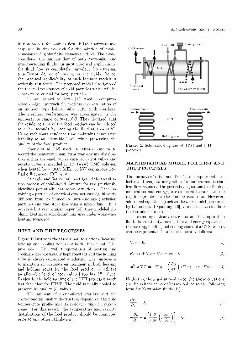
Figure 13 shows variations of sterility and qualityparameters with a volumetric ow rate (or Reynoldsnumber). Increasing the ow rate under laminarconditions initially decreases both sterility and qualityparameters due to residence time reduction. However,as the uid enters the turbulent region, both param-

Simulation of a CTS Process 37

Figure 13. Variations of sterility and quality parameterswith volumetric ow rate (heating zone wall temperature= 140�C).

eters encounter a sharp increase. The sterility thenslightly decreases as the volumetric ow rate increases,while the quality parameter severely decreases, as theReynolds number increases, because of a major de-crease in residence time. Figure 13 demonstrates thatan unpredicted transition from a laminar condition to aslightly turbulent situation should be avoided, since itcan drastically reduce the quality of the food product.

Simulation of CTS Process in the Presence ofSuspended Solid Particles

To the best of our knowledge, the e�ect of solidparticles in the simulation of CTS processes has notreceived su�cient attention in previous articles. Inmany practical situations, the sterilized uid containsa considerable amount of small solid particles (such asfat, gelatin and starch), which can coagulate togetherand produce relatively large particles [24]. The sporesor other pathological macroorganisms may be trappedin the center of such coagulated particles. Evidently,the amount of accumulated sterility will drop sharplyfor such entrapped spores (because of the solid particleheat resistance). Furthermore, these particles mayundergo di�erent trajectories in a turbulent ow. Thee�ects of a particle trajectory and its heat transferresistance on both quality and sterility parameters areconsidered in the following sections.

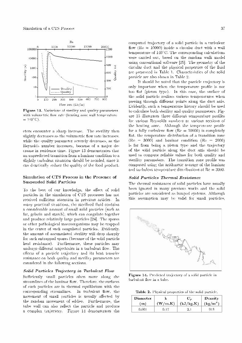
Solid Particles Trajectory in Turbulent FlowSu�ciently small particles often move along thestreamlines of the laminar ow. Therefore, the surfacesof such particles are in thermal equilibrium with thecorresponding streamlines. In turbulent ow, themovement of small particles is usually a�ected bythe random movement of eddies. Furthermore, thetube wall can also re ect the particle and producea complex trajectory. Figure 14 demonstrates the

computed trajectory of a solid particle in a turbulent ow (Re � 10000) inside a circular duct with a walltemperature of 140�C. The corresponding calculationswere carried out, based on the random walk modelusing conventional software [25]. The geometry of thecircular duct and the physical properties of the uidare presented in Table 1. Characteristics of the solidparticle are also shown in Table 2.

It should be noted that the particle trajectory isonly important when the temperature pro�le is nottoo at (piston type). In this case, the surface ofthe solid particle realizes various temperatures whenpassing through di�erent points along the duct axis.Evidently, such a temperature history should be usedto calculate both sterility and quality parameters. Fig-ure 15 illustrates three di�erent temperature pro�lesfor various Reynolds numbers at various sections ofthe heating zone. Although the temperature pro�lefor a fully turbulent ow (Re = 10000) is completely at, the temperature distribution of a transition zone(Re = 3000) and laminar condition (Re = 2000)is far from being a piston type and the trajectoryof the solid particle along the duct axis should beused to compute reliable values for both quality andsterility parameters. The transition zone pro�le wascomputed using the arithmetic average of the laminarand turbulent temperature distributions at Re = 3000.

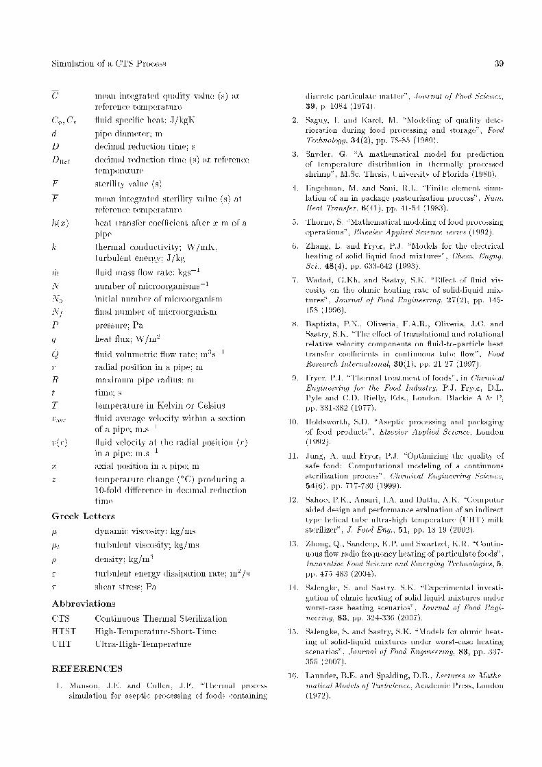
Solid Particles Thermal ResistanceThe thermal resistances of solid particles have usuallybeen ignored in many previous works and the solidparticles are considered as lumped systems. Althoughthis assumption may be valid for small particles,

Figure 14. Predicted trajectory of a solid particle inturbulent ow in a tube.

Table 2. Physical properties of the solid particle.

Diameter(m)

k(W/m.K)

Cp(kJ/kg.K)

Density(kg/m3)

0.001 0.17 2.1 918

38 A. Shahsavand and Y. Nozari

Figure 15. Heating zone radial temperature pro�les forvarious ow regimes.

distributed models are required to take account of thethermal resistance of relatively large solid particles. Itis clear that the center temperature of such particles(d > 100 �m) is much lower than their surface tem-peratures. Therefore, the lumped assumption yields tomisleadingly large sterility values.

Figure 16 compares the distributed model pre-dictions of central temperatures for various sizes ofsolid particles with a corresponding lumped model.The wall temperature of the heating zone and the uid Reynolds number were considered as 140�C and10000, respectively. It is clearly shown that the centraltemperature of the large particles (d > 3 mm) ismuch lower than the surface temperature (lumpedsystems). A large number of food products containsuspended solids with various sizes between 3 to 20millimeters [26].

The solid particle trajectory and the correspond-ing temperature history were computed �rst via theconventional software. The central temperatures andthe corresponding sterility values were then calculatedusing in-house software. Figure 17 emphasizes that the

Figure 16. Comparison of central temperaturescomputed via lumped and distributed models(Tw = 413 K).

Figure 17. Comparison of sterility values computed vialumped and distributed models (Tw = 413 K).

actual sterility received at the center of a large solidparticle is much smaller than that predicted by thelumped assumption.

CONCLUSIONS

Simulations of CTS processes were considered for bothlaminar and turbulent conditions. It was clearly shownthat for laminar ow, the �nite di�erence methodperforms adequately. It was also illustrated that simpleheuristics of (Vmax � Tbulk) and (Vaverage � Tcenter)provide the best predictions compared to the exactsolution of the laminar situation. Furthermore, usinga mixer at the entrance of the holding zone (whilekeeping other parameters constant) leads to a sharpincrease in the sterility value, while decreasing thequality destruction.

A relatively simple empirical method, based ona dimensionless Nusselt number, was presented forturbulent conditions, and provided practically the sameresults compared to the more sophisticated method ofthe control volume technique. It was also illustratedthat during laminar operations, great care should betaken to avoid entering the turbulent region. Such acondition drastically reduces the quality of the foodproduct.

Using the turbulent condition also critically re-duces the length of both heating and holding zonesand, hence, signi�cantly preserves the quality of thefood product. The trajectories of solid particlesin a transitionally turbulent ow are proved to beimportant and it was emphasized that the thermalresistances of relatively large solid particles should bealso considered for the calculation of both sterility andquality parameters.

NOMENCLATURE

C quality value (s)

Simulation of a CTS Process 39

C mean integrated quality value (s) atreference temperature

Cp; Cv uid speci�c heat; J/kgKd pipe diameter; mD decimal reduction time; sDRef decimal reduction time (s) at reference

temperatureF sterility value (s)

F mean integrated sterility value (s) atreference temperature

h(x) heat transfer coe�cient after x m of apipe

k thermal conductivity; W/mK,turbulent energy; J/kg

_m uid mass ow rate; kgs�1

N number of microorganisms�1

N0 initial number of microorganismNf �nal number of microorganismP pressure; Paq heat ux; W/m2

_Q uid volumetric ow rate; m3s�1

r radial position in a pipe; mR maximum pipe radius; mt time; sT temperature in Kelvin or Celsiusvave uid average velocity within a section

of a pipe; m.s�1

v(r) uid velocity at the radial position (r)in a pipe; m.s�1

x axial position in a pipe; mz temperature change (�C) producing a

10-fold di�erence in decimal reductiontime

Greek Letters

� dynamic viscosity; kg/ms�t turbulent viscosity; kg/ms� density; kg/m3

" turbulent energy dissipation rate; m2/s� shear stress; Pa

Abbreviations

CTS Continuous Thermal SterilizationHTST High-Temperature-Short-TimeUHT Ultra-High-Temperature

REFERENCES

1. Manson, J.E. and Cullen, J.F. \Thermal processsimulation for aseptic processing of foods containing

discrete particulate matter", Journal of Food Science,39, p. 1084 (1974).

2. Saguy, I. and Karel, M. \Modeling of quality dete-rioration during food processing and storage", FoodTechnology, 34(2), pp. 78-85 (1980).

3. Snyder, G. \A mathematical model for predictionof temperature distribution in thermally processedshrimp", M.Sc. Thesis, University of Florida (1986).

4. Engelman, M. and Sani, R.L. \Finite element simu-lation of an in-package pasteurization process", Num.Heat Transfer, 6(41), pp. 41-54 (1983).

5. Thorne, S. \Mathematical modeling of food processingoperations", Elsevier Applied Science series (1992).

6. Zhang, L. and Fryer, P.J. \Models for the electricalheating of solid liquid food mixtures", Chem. Engng.Sci., 48(4), pp. 633-642 (1993).

7. Wadad, G.Kh. and Sastry, S.K. \E�ect of uid vis-cosity on the ohmic heating rate of solid-liquid mix-tures", Journal of Food Engineering, 27(2), pp. 145-158 (1996).

8. Baptista, P.N., Oliveria, F.A.R., Oliveria, J.C. andSastry, S.K. \The e�ect of translational and rotationalrelative velocity components on uid-to-particle heattransfer coe�cients in continuous tube ow", FoodResearch International, 30(1), pp. 21-27 (1997).

9. Fryer, P.J. \Thermal treatment of foods", in ChemicalEngineering for the Food Industry, P.J. Fryer, D.L.Pyle and C.D. Rielly, Eds., London, Blackie A & P,pp. 331-382 (1977).

10. Holdsworth, S.D. \Aseptic processing and packagingof food products", Elsevier Applied Science, London(1992).

11. Jung, A. and Fryer, P.J. \Optimizing the quality ofsafe food: Computational modeling of a continuoussterilization process", Chemical Engineering Science,54(6), pp. 717-730 (1999).

12. Sahoo, P.K., Ansari, I.A. and Datta, A.K. \Computeraided design and performance evaluation of an indirecttype helical tube ultra-high temperature (UHT) milksterilizer", J. Food Eng., 51, pp. 13-19 (2002).

13. Zhong, Q., Sandeep, K.P. and Swartzel, K.R. \Contin-uous ow radio frequency heating of particulate foods",Innovative Food Science and Emerging Technologies, 5,pp. 475-483 (2004).

14. Salengke, S. and Sastry, S.K. \Experimental investi-gation of ohmic heating of solid-liquid mixtures underworst-case heating scenarios", Journal of Food Engi-neering, 83, pp. 324-336 (2007).

15. Salengke, S. and Sastry, S.K. \Models for ohmic heat-ing of solid-liquid mixtures under worst-case heatingscenarios", Journal of Food Engineering, 83, pp. 337-355 (2007).

16. Launder, B.E. and Spalding, D.B., Lectures in Mathe-matical Models of Turbulence, Academic Press, London(1972).

40 A. Shahsavand and Y. Nozari

17. Bird, R.B., Stewart, W.E. and Lightfoot, E.N., Trans-port Phenomena, 2nd Ed., John Wiley & Sons (2002).

18. Acrivos, A. \The extended Graetz problem at lowP�eclet numbers", Appl. Sci. Res., 36, p. 35 (1980).

19. Papoutsakis, E., Ramkrishna, D. and Lim, H.C. \Theextended Graetz problem with Dirichlet wall boundaryconditions", Appl. Sci. Res., 36, p. 13 (1980).

20. Nozari, Y. \Simulation of continuous thermal steril-ization process", M.Sc. Thesis, Ferdowsi University,Mashad, Iran (2006).

21. Holman, J.P., Heat Transfer, 8th Ed., McGraw Hill,NY (1997).

22. Loncin, M. and Merson, R.L., Food Engineering,Selected Applications, Academic Press, London (1979).

23. Dang, C. and Hihara, E. \In-tube cooling heat transfer

of supercritical carbon dioxide. Part 2. Comparison ofnumerical calculation with di�erent turbulence mod-els", Internatinal Journal of Refrigeration, 27, pp. 748-760 (2004).

24. Fellows, P.J., Food Processing Technology Principlesand Practice, 2nd Ed., Woodhead Publishing in FoodScience and Technology (2002).

25. Zevenhoven, R. \Particle/turbulence interactions andCFD modeling of dilute suspensions", The CombustionInstitute Topical Meeting on Modeling of Combustionand Combustion Processes, Finland (2000).

26. Mankad, S. and Fryer, P.J. \A heterogeneous owmodel for the e�ect of slip and ow velocities onfood sterilizer design", Chemical Engineering Science,52(12), pp. 1835-1843 (1977).