Embed Size (px)
Citation preview

Master Class, Washington University, Nov 16 Introduction and Computational Model
THEORY OF SYSTEMSMODELING AND ANALYSIS
1
Henny SipmaStanford University
Master classWashington University at St Louis
November 16, 2006
1

Master Class, Washington University, Nov 16 Introduction and Computational Model
COURSE OUTLINE
2
8:37 - 10:00 Introduction -- Computational model Fair transition systems -- Temporal logic
10:07 - 11:30 Verification methods Rules -- Diagrams -- Abstraction Traditional static analysis methods
1:07 - 2:30 Constraint-based static analysis methods Real-time and hybrid systems
2:37 - 4:00 Formalization of middleware services: Event correlation
2

Master Class, Washington University, Nov 16 Introduction and Computational Model
My background
3
B.S. Chemistry, Groningen, The NetherlandsM.S. Chemical Engineering, idem
7 years as Control Engineer with Shell in The Netherlands, Singapore and Houston, TX
M.S. Computer Science, Stanford
Ph.D. Computer Science, Stanford
Sr. Research Associate at Stanford since 2000
3

Master Class, Washington University, Nov 16 Introduction and Computational Model
Research Interests
4
• Static Analysis• Constraint-based reasoning
• Runtime Analysis• Monitoring of temporal properties
• Decision Procedures• Data structures
• Formalization of Middleware services• Event Correlation• Deadlock Avoidance
4
Master Class, Washington University, Nov 16 Introduction and Computational Model
I. Introduction
5
5

Master Class, Washington University, Nov 16 Introduction and Computational Model
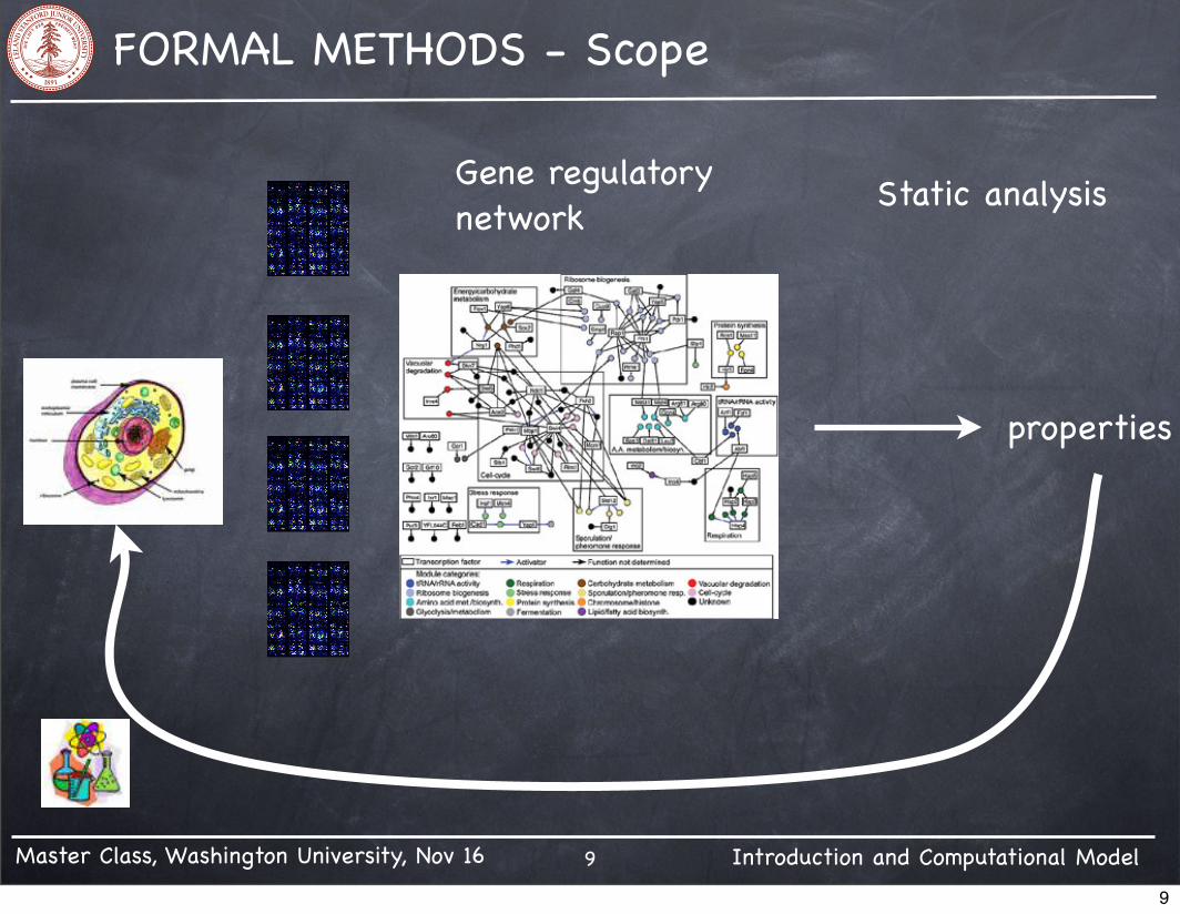
Reactive Systems
6
Continuous interaction with the environment
time
Observable throughout its execution
6

Master Class, Washington University, Nov 16 Introduction and Computational Model
OBJECTIVE: Analysis of System Behaviors
THEORY: Logic + Automata
COMPONENTS: Model (+ Specification)
METHODS: Deductive and Algorithmic
7
7

Master Class, Washington University, Nov 16 Introduction and Computational Model
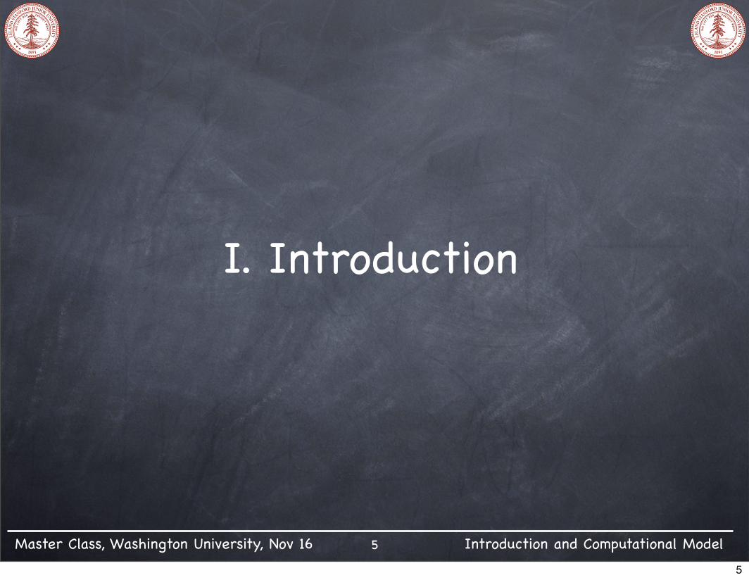
FORMAL METHODS - Scope
8
Complex system Natural-languagespecification
Model Formalspecification
Formal Verification
8
Master Class, Washington University, Nov 16 Introduction and Computational Model
FORMAL METHODS - Scope
9
Static analysisGene regulatorynetwork
properties
9

Master Class, Washington University, Nov 16 Introduction and Computational Model
FORMALIZATION OF MIDDLEWARE SERVICES
10
OS KernelOS I/O subsystemNetwork Adapters
ORB Core
ORB Services
Event NotificationEvent CorrelationConcurrency
LoggingTradingScheduling
Deadlock AvoidanceLoad Balancing
OS KernelOS I/O subsystemNetwork Adapters
Application ApplicationApplication
10
Master Class, Washington University, Nov 16 Introduction and Computational Model
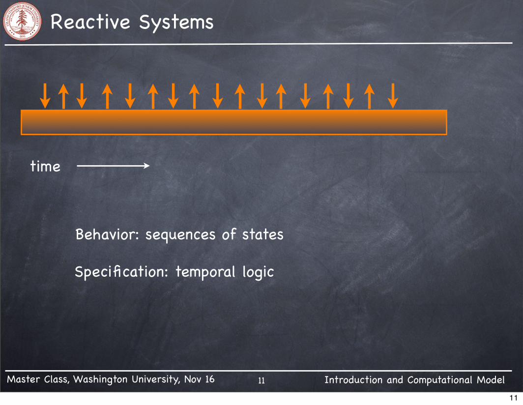
Reactive Systems
11
time
Behavior: sequences of states
Specification: temporal logic
11

Master Class, Washington University, Nov 16 Introduction and Computational Model
Verification process
12
Fair transitionsystem
System specificationSystem description
Verification techniques
Temporal logicformula
Proof Counterexample
12

Master Class, Washington University, Nov 16 Introduction and Computational Model
Static analysis (traditional)
13
Fair transitionsystem
System description
Symbolic simulation
abstractdomain
Invariants
13

Master Class, Washington University, Nov 16 Introduction and Computational Model
templateproperty
Static analysis (constraint-based)
14
Fair transitionsystem
System description
System of constraints
Invariants Proof of terminationtemporal properties
14
Master Class, Washington University, Nov 16 Introduction and Computational Model
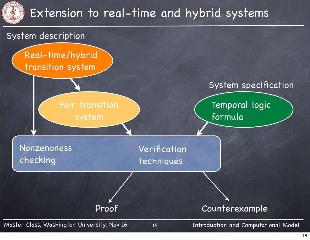
Extension to real-time and hybrid systems
15
System specification
System description
Verification techniques
Proof Counterexample
Real-time/hybridtransition system
Nonzenonesschecking
Fair transitionsystem
Temporal logicformula
15

Master Class, Washington University, Nov 16 Introduction and Computational Model
Verification techniques (1)
16
Algorithmic: exhaustive search for counterexamples
Issues: • state space explosion problem• efficient representations• applicable to finite-state systems only
16
Master Class, Washington University, Nov 16 Introduction and Computational Model
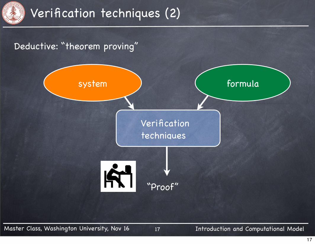
Verification techniques (2)
17
Deductive: “theorem proving”
system
Verification techniques
formula
“Proof”
17

Master Class, Washington University, Nov 16 Introduction and Computational Model
Verification techniques (2)
18
Deductive: “theorem proving”
system
Verification techniques
formula
100s/1000s/10,000s of first-order verification conditions
Decision procedures
18

Master Class, Washington University, Nov 16 Introduction and Computational Model
II. COMPUTATIONAL MODEL
19
• Fair transition systems• Temporal logic: LTL
Reference: Zohar Manna, Amir Pnueli, Temporal Verification of Reactive Systems: Safety, Springer-Verlag, 1995.
19
Master Class, Washington University, Nov 16 Introduction and Computational Model
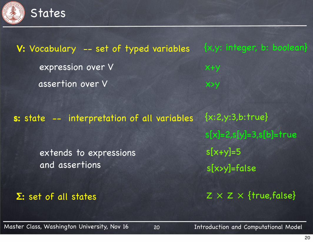
States
20
V: Vocabulary -- set of typed variables
expression over V
assertion over V
{x,y: integer, b: boolean}
x+y
x>y
s: state -- interpretation of all variables
extends to expressions and assertions
{x:2,y:3,b:true}
s[x]=2,s[y]=3,s[b]=true
s[x+y]=5
s[x>y]=false
Σ: set of all states Z × Z × {true,false}
20

Master Class, Washington University, Nov 16 Introduction and Computational Model
System Description: Fair transition systems
21
Φ: < V , Θ , T , F >
Set of typed variables
Initial condition: first-order formula
Set of transitions
Fairness condition
Example: x=0 ∧ y=0
Compact first-order representation of all sequences of statesthat can be generated by a system
Example: {x,y} F⊆T
21

Master Class, Washington University, Nov 16 Introduction and Computational Model
Transitions
22
T: finite set of transitions
τ∈T: Σ → 2Σ
s
Σ τ-successors of sτ(s):
.
represented by a transition relation ρτ(V,V’)
V : values of variables in the current stateV’: values of variables in the next state
Example:
ρτ: x’=x+1 ⋁ x’=x+2
τ(<x:2>) = {<x:3>,<x:4>}
22

Master Class, Washington University, Nov 16 Introduction and Computational Model
Runs and Computations
23
Infinite sequence of states
σ: s0 s1 s2 s3 s4 .............
is a run of Φ if
☛ Initiality: s0 ⊧ Θ (s0 is an initial state)
☛ Consecution: for all i > 0
si+1 is a τ-successor of si
for some τ ∈ T
s0 s1 s2 s3 ....
τ τ τ τ
23

Master Class, Washington University, Nov 16 Introduction and Computational Model
Runs and Computations
24
Infinite sequence of states
σ: s0 s1 s2 s3 s4 .............
is a computation of Φ if
☛ σ is a run☛ Justice: for each τ∈F
if τ is enabled infinitely often in σit is taken infinitely often in σ
τ is enabled on Si: τ(si) ≠ ∅τ is taken on si: si+1 ∈ τ(si)
24

Master Class, Washington University, Nov 16 Introduction and Computational Model
Runs and Computations: Example
25
V: {x:integer}Θ: x=0
T: {τ1, τ2, τ3} withρτ1 : x’=x+1 ⋁ x’=x+3ρτ2 : x’=x+2 ⋁ x’=2xρτ3 : x’=x
{F: {τ1, τ2}
σ1: 0, 1, 2, 3, 4, 5, 6, 7, .............
σ2: 0, 0, 0, 0, 0, 0, 0, 0 .............
σ3: 0, 2, 4, 8, 16, 32, .............
σ4: 0, 1, 1, 3, 3, 5, 5, 7, 7, .............
σ5: 1, 2, 3, 5, 6, 8, 9, 11, .............
Run? Computation?
✓✓✓✓
××××××
25

Master Class, Washington University, Nov 16 Introduction and Computational Model
Runs and Computations: Example
26
V: {x:integer}Θ: x=0
T: {τ1, τ2, τ3} withρτ1 : (x=0 ⋁ x=1) ⋀ (x’=x+1 ⋁ x’=x+3)ρτ2 : x’=x+2 ⋁ x’=2xρτ3 : x’=x
{F: {τ1, τ2}
σ1: 0, 1, 2, 3, 4, 5, 6, 7, .............
σ2: 0, 0, 0, 0, 0, 0, 0, 0 .............
σ3: 0, 2, 4, 8, 16, 32, .............
σ4: 0, 1, 1, 3, 3, 5, 5, 7, 7, .............
σ5: 1, 2, 3, 5, 6, 8, 9, 11, .............
Run? Computation?
✓✓✓✓
✓
✓
××
×××
26

Master Class, Washington University, Nov 16 Introduction and Computational Model
System Description: Summary
27
Fair transition system: Φ: < V , Θ , T , F >
Run: Initiality + Consecution
Computation: Run + Justice
L(Φ): all computations of Φ
(all sequences of states that satisfy Initiality, Consecution and Justice)
“Behavior of the program”
27

Master Class, Washington University, Nov 16 Introduction and Computational Model
Reachable state space
28
state s is Φ-reachable if it appears in some Φ-computation
σ: s0 s1 s2 s3 s4 .............
system Φ is finite-state if the set of Φ-reachable states is finite
Notation: Σ : state spaceΣΦ⊳: Φ-reachable state space
Example:V: {b1, b2}Θ: b1⋀b2
T: {τ} with ρτ: b1’=¬b1⋀b2’=¬b2
Σ = {<t,t>,<t,f>,<f,t>,<f,f>}
ΣΦ⊳ = {<t,t>,<f,f>}
28

Master Class, Washington University, Nov 16 Introduction and Computational Model
Reachable state space
29
state s is Φ-reachable if it appears in some Φ-computation
σ: s0 s1 s2 s3 s4 .............
system Φ is finite-state if the set of Φ-reachable states is finite
Notation: Σ : state spaceΣΦ⊳: Φ-reachable state space
Example:V: {x}Θ: x=0T: {τ} with ρτ: x=0 ⋀ x’=x+1
Σ = N
ΣΦ⊳ = {x:0, x:1}
29

Master Class, Washington University, Nov 16 Introduction and Computational Model
Reachable state space
30
state s is Φ-reachable if it appears in some Φ-computation
σ: s0 s1 s2 s3 s4 .............
system Φ is finite-state if the set of Φ-reachable states is finite
Notation: Σ : state spaceΣΦ⊳: Φ-reachable state space
Example:V: {x}Θ: 0 ≤ x ≤ MT: {τ1,τ2} with ρτ1: odd(x) ⋀ x’=3x+1 ρτ2: even(x) ⋀ x’=x/2
Σ = N
ΣΦ⊳ = ?
30
Master Class, Washington University, Nov 16 Introduction and Computational Model
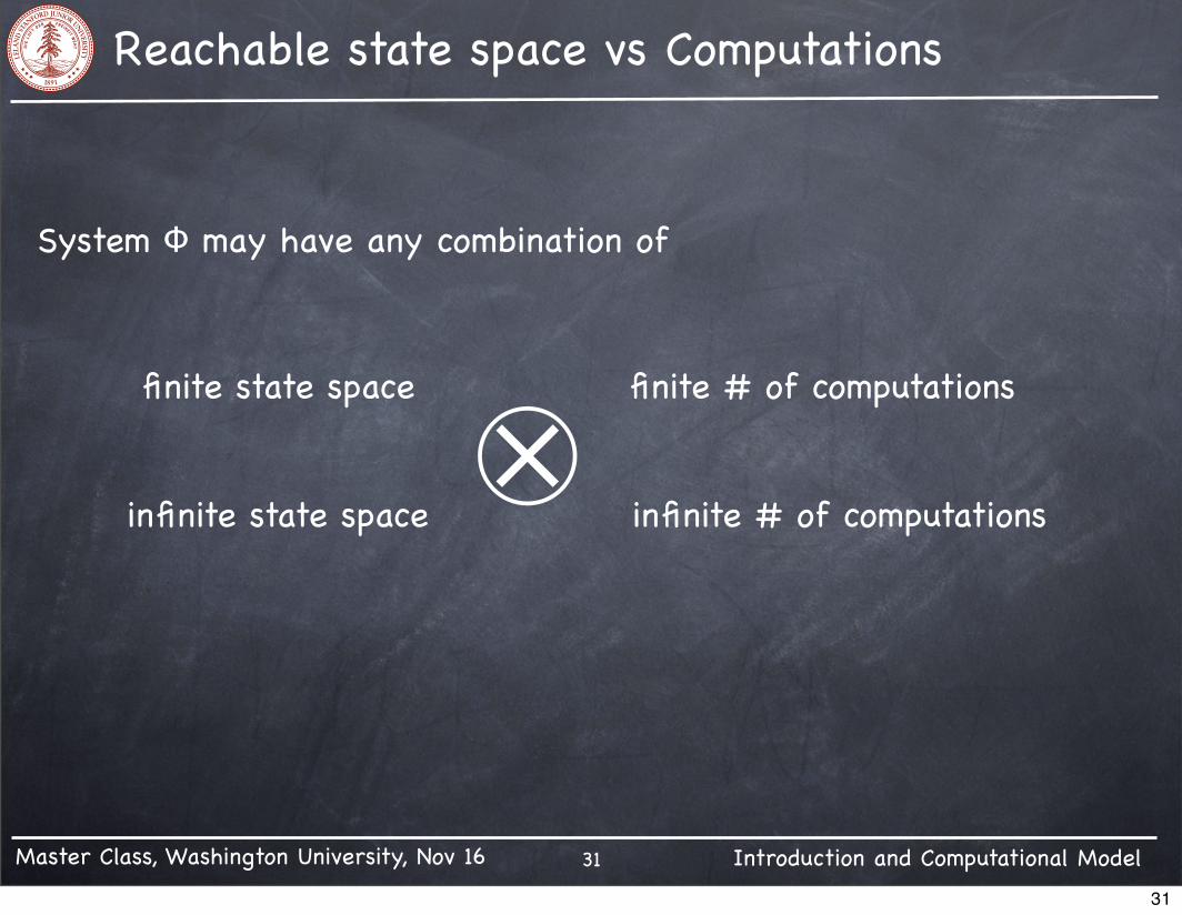
Reachable state space vs Computations
31
⊗finite state space
infinite state space
finite # of computations
infinite # of computations
System Φ may have any combination of
31

Master Class, Washington University, Nov 16 Introduction and Computational Model
II. COMPUTATIONAL MODEL
32
• Fair transition systems• Temporal logic: LTL
Reference: Zohar Manna, Amir Pnueli, Temporal Verification of Reactive Systems: Safety, Springer-Verlag, 1995.
32

Master Class, Washington University, Nov 16 Introduction and Computational Model
Temporal Logic
33
Language that specifies the behavior of a reactive system
System Φ ---------------------------- System behavior: L(Φ)
Temporal formula φ --- Sequences of states that satisfy φ: L(φ)
System Φ satisfies specification φ
Φ ⊨ φif L(Φ) ⊆ L(φ)
33

Master Class, Washington University, Nov 16 Introduction and Computational Model
Temporal logic
34
System Φ satisfies specification φ
Φ ⊨ φif L(Φ) ⊆ L(φ)
Σ∞
L(φ)L(Φ)
34

Master Class, Washington University, Nov 16 Introduction and Computational Model
First-order logic --- Temporal logic
35
Temporal logic
models are sequences of states
temporal formula φrepresents
the set of sequences of statesfor which φ is true
First-order logic
models are states
assertion p represents
the set of states for which p is true
<x:3,y:1> ⊫ x > y <s0 s1 s2 s3 ....> ⊨ φ
35

Master Class, Washington University, Nov 16 Introduction and Computational Model
Temporal logic: underlying assertion language
36
Assertion language A:
first-order language over system variables(+ theories for their domains)
Formulas in A: state formulas (aka assertions)
evaluated over a single state
s ⊫ p iff s[p] = true
p holds at ss satisfies ss is a p-state
Example: s: <x:4, y:1>
s ⊫ x=0 ⋁ y=1s ⊫ x > ys ⊫ x = y+3s ⊯ odd(x)
36

Master Class, Washington University, Nov 16 Introduction and Computational Model
Temporal logic: underlying assertion language
37
x>0x>5
Σx2< 100
Assertions represent sets of states
37
Master Class, Washington University, Nov 16 Introduction and Computational Model
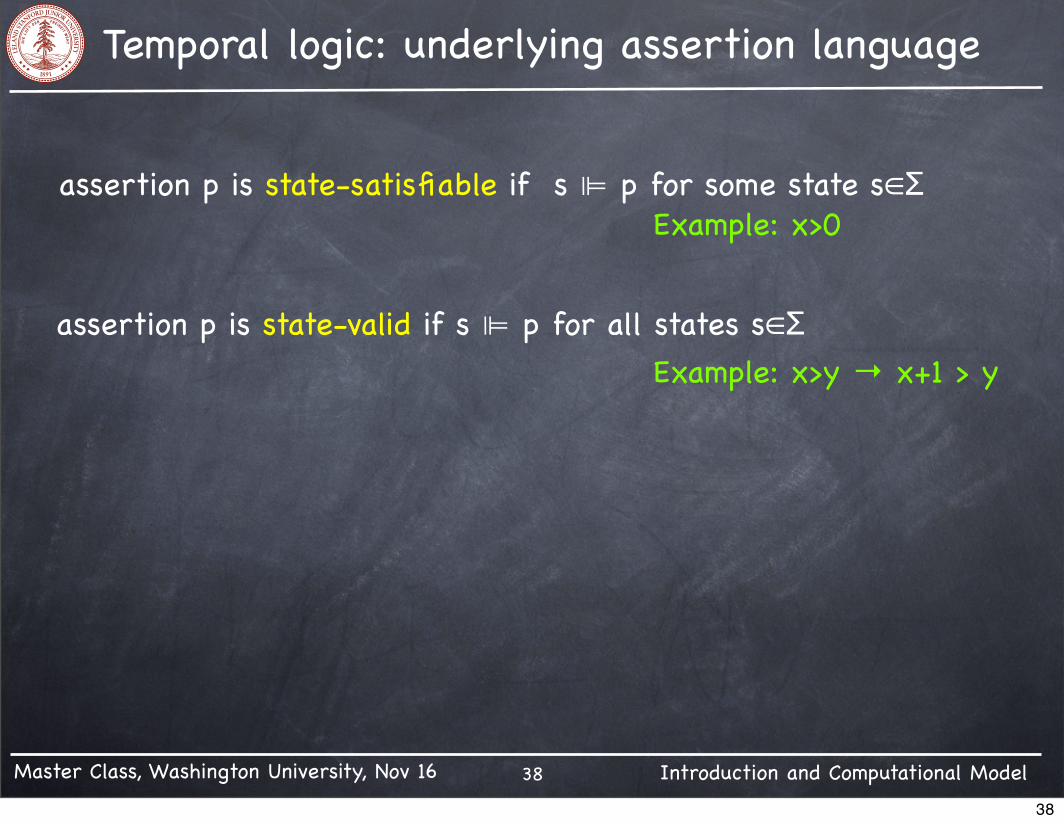
Temporal logic: underlying assertion language
38
assertion p is state-satisfiable if s ⊫ p for some state s∈Σ
assertion p is state-valid if s ⊫ p for all states s∈Σ Example: x>y → x+1 > y
Example: x>0
38
Master Class, Washington University, Nov 16 Introduction and Computational Model
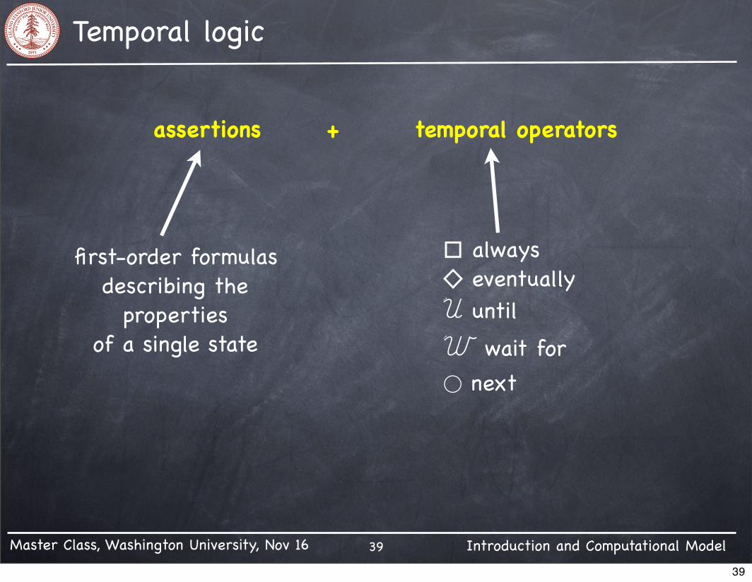
Temporal logic
39
assertions + temporal operators
first-order formulasdescribing the
propertiesof a single state
□ always◇ eventuallyU untilW wait for◯ next
39
Master Class, Washington University, Nov 16 Introduction and Computational Model
Temporal logic: safety versus liveness
40
Safety property: “nothing bad will happen”
Liveness property: “something good will happen”
it will not happen that the train is in the crossing whilethe gates are open
the train will eventually be able to pass the crossing
40

Master Class, Washington University, Nov 16 Introduction and Computational Model
Temporal logic -- informal
41
□p
p p p p p p p p p p p p p p p p
◇pp
pUqp p p p p p p q
◯pp
present
41

Master Class, Washington University, Nov 16 Introduction and Computational Model
Temporal logic: syntax
42
☛ every assertion is a temporal formula
☛ if φ and ψ are temporal formulas, so are
¬φboolean combinations: φ⋀ψ φ⋁ψ φ→ψ
temporal combinations: ◇φ □φ ◯φ φUψ φWψ
Examples:
□(x=0 → ◇(x>0))pUq → ◇q
42
Master Class, Washington University, Nov 16 Introduction and Computational Model
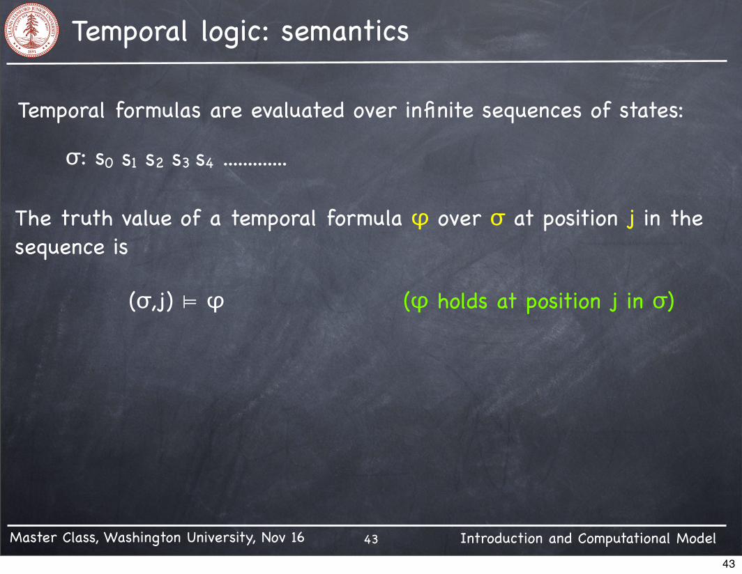
Temporal logic: semantics
43
Temporal formulas are evaluated over infinite sequences of states:
σ: s0 s1 s2 s3 s4 .............
The truth value of a temporal formula φ over σ at position j in the sequence is
(σ,j) ⊨ φ (φ holds at position j in σ)
43

Master Class, Washington University, Nov 16 Introduction and Computational Model
Temporal logic: semantics
44
☛ if φ is a state formula p
(σ,j) ⊨ φ iff sj ⊫ p
σ<x>: 4, 3, 1, 7, 5, 8, 0, 0, 0, 0Example:
(σ,3) ⊨ x > 6(σ,6) ⊨ x=0
<x:7> ⊫ x > 6
☛ if φ is a temporal formula of the form (boolean operators)
(σ,j) ⊨ ¬ψ iff (σ,j) ⊭ ψ
(σ,j) ⊨ ψ ⋁ χ iff (σ,j) ⊨ ψ or (σ,j) ⊨ χ
44

Master Class, Washington University, Nov 16 Introduction and Computational Model
Temporal logic: semantics
45
☛ if φ is a temporal formula of the form (temporal operators)
(σ,j) ⊨ □ψ iff for all k≥j, (σ,j) ⊫ ψ
j
ψ ψ ψ ψ ψ ψ ψ
(σ,j) ⊨ ◇ψ iff for some k≥j, (σ,j) ⊫ ψ
j
ψ
45

Master Class, Washington University, Nov 16 Introduction and Computational Model
Temporal logic: semantics
46
☛ if φ is a temporal formula of the form (temporal operators)
(σ,j) ⊨ ψUχ iff for some k≥j, (σ,j) ⊫ χ and for all i, j≤i<k, (σ,j) ⊫ ψ
j
ψ χ
k
(σ,j) ⊨ ψWχ iff (σ,j) ⊨ ψUχ or (σ,j) ⊨ □ψ
(σ,j) ⊨ ◯ψ iff (σ,j+1) ⊨ ψ
j
ψ
j+1
ψψψψψ
46

Master Class, Washington University, Nov 16 Introduction and Computational Model
Temporal logic: semantics
47
A sequence of states σ satisfies a temporal formula φ
σ ⊨ φ iff (σ,0) ⊨ φ
47

Master Class, Washington University, Nov 16 Introduction and Computational Model
Temporal logic formulas: examples
48
p → ◇q
if initially p then eventually q
p q
□(p → ◇q)p p p q p pq q
every p is eventually followed by a q
□(p → ◯p)p p p
once p, always p
p p p p p p p p p p p
48

Master Class, Washington University, Nov 16 Introduction and Computational Model
Temporal logic formulas: examples
49
□◇pp p p p p p p
every position is eventually followed by a p“infinitely often p”
◇□pp p p p
eventually always p
p p p p p p p p
if there are infinitely many p’s then there are infinitely many q’s
□◇p → □◇q
49

Master Class, Washington University, Nov 16 Introduction and Computational Model
Temporal logic formulas: examples
50
Nested waiting-for formulas: q1W(q2W(q3Wq4))
intervals of continuous qi:q1 q1 q1 q1 q2 q2 q2 q3 q3 q3q3q4
possibly empty interval:q1 q1 q1 q1 q3 q3 q3 q3 q3 q3q3q4
possibly infinite interval:q1 q1 q1 q1 q2 q2 q2 q3 q3 q3q3q3 q3 q3 q3 q3 q3 q3 q3
50

Master Class, Washington University, Nov 16 Introduction and Computational Model
Temporal logic: summary
51
For temporal formula φ, sequence of states σ, position j≥0:
(σ,j) ⊨ φφ holds at position j in σ
σ satisfies φ at jj is a φ-position in σ
For temporal formula φ and sequence of states σ
(σ,0) ⊨ φσ ⊨ φ iffφ holds on σσ satisfies φ
51

Master Class, Washington University, Nov 16 Introduction and Computational Model
Temporal logic: satisfiability and validity
52
For temporal formula φ
☛ φ is satisfiable if σ ⊨ φ for some sequence of states σ
☛ φ is valid if σ ⊨ φ for all sequences of states σ
□(x>0) ◇(x>5)
Σ∞
(x>0)U(x>5)
52

Master Class, Washington University, Nov 16 Introduction and Computational Model
Temporal logic: satisfiability/validity examples
53
◇(x=0)
satisfiable? valid?
◇(x=0) ⋁ □(x≠0)
◇(x=0) ⋀ □(x≠0)
◇(x=0) ⋀ ◇(x=1)
◇(x=0) ⋁ ◇(x=1)
◇□p → □◇p
□◇p → ◇□p
pU(q⋀r) → (◇q ⋀ ◇r)
✓
✓ ✓
✓
✓
✓
✓
✓ ✓
✓
×
× ×
×
×
×
53

Master Class, Washington University, Nov 16 Introduction and Computational Model
Temporal logic: Equivalences
54
Temporal formulas φ, ψ are congruent φ ≈ ψif □(φ ↔ ψ) is valid
φ and ψ have the same truth value at all positions in all models
□(p ⋀ q)
□(p ⋁ q)
congruent?
□p ⋀ □q
□p ⋁ □q
pU(q⋁r) pUq ⋁ pUr
pU(q⋀r) pUq ⋀ pUr
✓
✓
×
×
54

Master Class, Washington University, Nov 16 Introduction and Computational Model
Temporal logic: Expansions
55
□φ ≈ φ ⋀ ◯□φ
◇φ ≈ φ ⋁ ◯◇φ
φUψ ≈ ψ ⋁ (φ ⋀ ◯(φUψ))
Used in checking temporal formulas in model checking
55

Master Class, Washington University, Nov 16 Introduction and Computational Model
Expressiveness
56
Some properties cannot be expressed in LTL:
☛ p is true, if at all, only at even positions
Not specified by
∃t ( t ⋀ □(t ↔ ¬◯t) ⋀ □(p → t) )
p ⋀ □( p → ◯◯p ) or p ⋀ □( p ↔ ¬◯p )
requires quantification
56
Master Class, Washington University, Nov 16 Introduction and Computational Model
Temporal logic vs First-order logic
57
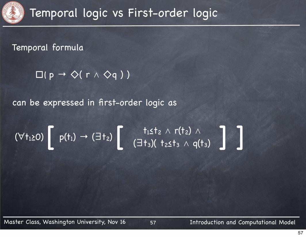
Temporal formula
□( p → ◇( r ⋀ ◇q ) )
can be expressed in first-order logic as
(∀t1≥0) [ p(t1) → (∃t2) [ t1≤t2 ⋀ r(t2) ⋀(∃t3)( t2≤t3 ⋀ q(t3) ] ]
57