Embed Size (px)
Citation preview

THEORY OF QUANTUM DEGENERATE GASES
BY
ERICH JON MUELLER
B.S., University of British Columbia, 1996
THESIS
Submitted in partial fulfillment of the requirementsfor the degree of Doctor of Philosophy in Physics
in the Graduate College of theUniversity of Illinois at Urbana-Champaign, 2001
Urbana, Illinois

c© Copyright by Erich Jon Mueller, 2001

THEORY OF QUANTUM DEGENERATE GASES
Erich Jon Mueller, Ph.D.Department of Physics
University of Illinois at Urbana-Champaign, 2001Gordon Baym, Advisor
Motivated by experiments on cold alkali atoms, I present a theoretical study of weakly
interacting quantum degenerate particles. These experiments observe a wide range
of phenomena and consequently this thesis has a broad scope, involving issues of
coherence, stability, superfluidity, and kinetics. I explore six topics which exemplify
the rich and exciting physics of cold alkali atoms: first, the effect of interactions on the
transition temperature of a dilute Bose gas; second, the connection between broken
non-gauge symmetries and the appearance of multiple condensates in a Bose gas;
third, the role of thermally activated “phase slip” events in destroying superfluidity
near the critical temperature of a Bose gas; fourth, mechanical instabilities in clouds
of attractive bosons; fifth, the kinetics of a gas of partially condensed atoms; and
sixth, the nonlinear optical properties of an atomic gases.
iii
Acknowledgments
This Ph.D. thesis was a five year project, and it is rather daunting to enumerate all of
the people who played important roles in its production. I should begin by thanking
my wife Sue, with whom I am looking forward to a wonderful life, and her family
who have been very welcoming. I also want to thank my parents for their continued
support.
I have had several important mentors here at UIUC. Gordon Baym, my advisor,
who has infinite patience, and who has tried his best to show me how physics is
done; Paul Goldbart, who walked me through my first research project, provided
much encouragement, and who runs a truly unique and wonderful seminar series, the
“meso meetings”; Tony Leggett, a keen mind, who has always given me kindly and
well thought out advice.
I have also benefited from the expert guidance of many physicists from all areas
of the world. Most of these people I met at one of three institutions. First, the
Institute for Theoretical Physics in Santa Barbara, directed by David Gross, where
in 1998 there was a program devoted to the study of Bose-Einstein Condensation. I
truly thank the organizers, Keith Burnett, Atac Imamoglu, and Tony Leggett, who
generously allowed me to spend over a month in Santa Barbara, and who contributed
some financial support. Second, the Laboratoire Kastler Brossel at the Ecole Normale
Superieure in Paris, where I spent six months in 1999. The trip, and the research
performed there, was facilitated by a cooperative agreement between the University of
Illinois at Urbana-Champaign and the Centre National de la Recherche Scientifique.
The third institution is the idyllic Aspen Center for Physics which has hosted two
workshops on Bose condensation; one in 1999, and the other in 2001. I would like
to thank Jane Kelly and the other staff members at Aspen, as well as the organizers
of the workshops, Gordon Baym, Sandy Fetter, Jason Ho, Murray Holland, Randy
Hulet, Chris Pethick, Mark Kasevich, and Andre Ruckenstein
Of these researchers that I met while abroad, I would like to make a list of a
few who made a particular impression on me: James Anglin, Bernard Bernu, Eric
Braaten, Iacoppo Carusotto, Yvan Castin, Jean Dalibard, David Guery-Odelin, Allan
iv

Griffin, Brian Kennedy, Franck Laloe, Andre Ruckenstein, Alice Sinatra, Henk Stoof,
Gora Shlyapnikov, Fernando Sols, Masahito Ueda, Li You, Eugene Zaremba, and W.
Zurek.
Next I would like to acknowledge all of the students and postdoctoral fellows at
UIUC who have played an important role in my education. Many have been dear
friends, and it makes me sad to think that in the coming years I will see most of
them infrequently. These include: Sahel Ashhab, Johann Beda, Mark Dewing, Erik
Draeger, Peter Fleck, Nir Gov, Justin Gullingsrud, Kei Iida, Sımon Kosh, Carlos
Lobo, Yuli Lyana-Geller, Markus Holzmann, Anna Minguzzi, Burkhard Millitzer,
Sorin Paraoanu, Jim Popp, Dan Sheehy, John Shumway, Joerg Schmalian, Greg Sny-
der, Ivo Souza, Benoit Vanderheyden, Tim Wilkens, Rachel Wortis, Bob White, and
Ivar Zapata.
I would like to congratulate the experimentalists working with cold alkalis for the
ground breakikng work they have done. Even with all of the media attention they
have received, I think the true impact of what they have achieved is far in the future,
and has not even been hinted at. I have particularly enjoyed discussions with Randy
Hulet and Lene Hau.
Finally, I would like to thank the sources of my funding. For four years of my
Ph.D., I held a fellowship from Canada’s Natural Sciences and Engineering Research
Council, and from the University of Illinois. I have received support from the National
Science Foundation through grants NSF PHY94-21309, NSF PHY98-00978, and NSF
PHY00-98353. I am grateful for the financial aid provided by many of the conferences
and workshops which I have attended.
I apologize to the many people who I forgot to mention. Please blame my negli-
gence on the stress of writing a thesis, and not on any malice.
v

Contents
Chapter
1 General Introduction . . . . . . . . . . . . . . . . . . . . . . . . . . . . . . . . . . . . . . . . . . . . . 1
1.1 Overview . . . . . . . . . . . . . . . . . . . . . . . . . . . . . . . . . . 1
1.1.1 Phase transition . . . . . . . . . . . . . . . . . . . . . . . . . . 1
1.1.2 Fragmentation . . . . . . . . . . . . . . . . . . . . . . . . . . . 2
1.1.3 Persistent currents . . . . . . . . . . . . . . . . . . . . . . . . 2
1.1.4 Attractive interactions . . . . . . . . . . . . . . . . . . . . . . 2
1.1.5 Kinetic theory . . . . . . . . . . . . . . . . . . . . . . . . . . . 3
1.1.6 Electromagnetically induced transparency . . . . . . . . . . . 3
1.2 Experiments . . . . . . . . . . . . . . . . . . . . . . . . . . . . . . . . 3
1.2.1 Cooling and trapping . . . . . . . . . . . . . . . . . . . . . . . 4
1.2.2 Measurement procedures . . . . . . . . . . . . . . . . . . . . . 9
1.2.3 Fermions . . . . . . . . . . . . . . . . . . . . . . . . . . . . . . 11
1.2.4 Coherence experiments . . . . . . . . . . . . . . . . . . . . . . 12
1.2.5 Collapse of an attractive gas . . . . . . . . . . . . . . . . . . . 12
1.2.6 Spin relaxation . . . . . . . . . . . . . . . . . . . . . . . . . . 16
1.2.7 Electromagnetically induced transparency . . . . . . . . . . . 16
1.2.8 Feshbach resonance . . . . . . . . . . . . . . . . . . . . . . . . 16
2 Theory of the BEC Phase Transition . . . . . . . . . . . . . . . . . . . . . . . . . . . . . 18
2.1 Elementary description . . . . . . . . . . . . . . . . . . . . . . . . . . 20
2.1.1 Uniform gas . . . . . . . . . . . . . . . . . . . . . . . . . . . . 21
2.1.2 Harmonically trapped gas . . . . . . . . . . . . . . . . . . . . 23
2.2 Finite size effects . . . . . . . . . . . . . . . . . . . . . . . . . . . . . 23
2.2.1 Scaling in the ideal gas . . . . . . . . . . . . . . . . . . . . . . 25
2.2.2 Scaling in the canonical ensemble . . . . . . . . . . . . . . . . 28
2.3 Perturbative calculation of ∆T . . . . . . . . . . . . . . . . . . . . . . 31
2.3.1 Perturbation theory . . . . . . . . . . . . . . . . . . . . . . . . 31
vi

2.3.2 Calculation of ∆T . . . . . . . . . . . . . . . . . . . . . . . . 32
2.3.3 Connection with other approaches . . . . . . . . . . . . . . . . 33
2.4 ∆T in a harmonic trap . . . . . . . . . . . . . . . . . . . . . . . . . . 36
3 Fragmentation. . . . . . . . . . . . . . . . . . . . . . . . . . . . . . . . . . . . . . . . . . . . . . . . . . . . 39
3.1 Introduction . . . . . . . . . . . . . . . . . . . . . . . . . . . . . . . . 39
3.1.1 Bose-Einstein condensation and fragmentation . . . . . . . . . 40
3.1.2 An illustrative example . . . . . . . . . . . . . . . . . . . . . . 42
3.2 Discussion and generalization . . . . . . . . . . . . . . . . . . . . . . 45
3.2.1 Spontaneous symmetry breaking . . . . . . . . . . . . . . . . . 45
3.2.2 Measurement . . . . . . . . . . . . . . . . . . . . . . . . . . . 46
3.2.3 Commensurability . . . . . . . . . . . . . . . . . . . . . . . . 48
3.3 Other models . . . . . . . . . . . . . . . . . . . . . . . . . . . . . . . 49
3.3.1 Spin 1 . . . . . . . . . . . . . . . . . . . . . . . . . . . . . . . 49
3.3.2 Rotating attractive cloud . . . . . . . . . . . . . . . . . . . . . 52
3.3.3 Toroidal clouds . . . . . . . . . . . . . . . . . . . . . . . . . . 54
3.3.4 Multiple wells . . . . . . . . . . . . . . . . . . . . . . . . . . . 56
3.4 Further examples . . . . . . . . . . . . . . . . . . . . . . . . . . . . . 58
3.4.1 Phase separation . . . . . . . . . . . . . . . . . . . . . . . . . 58
3.4.2 Vortex structures . . . . . . . . . . . . . . . . . . . . . . . . . 59
3.5 Finite temperature . . . . . . . . . . . . . . . . . . . . . . . . . . . . 59
3.6 Summarizing remarks . . . . . . . . . . . . . . . . . . . . . . . . . . . 61
3.7 Mathematical details . . . . . . . . . . . . . . . . . . . . . . . . . . . 61
3.7.1 Josephson junctions . . . . . . . . . . . . . . . . . . . . . . . . 61
3.7.2 Distinguishing singly and multiply condensed states. . . . . . 65
4 Persistent Currents. . . . . . . . . . . . . . . . . . . . . . . . . . . . . . . . . . . . . . . . . . . . . . . 69
4.1 Introduction . . . . . . . . . . . . . . . . . . . . . . . . . . . . . . . . 69
4.2 Gross Pitaevskii functional . . . . . . . . . . . . . . . . . . . . . . . . 70
4.3 Thermally activated processes . . . . . . . . . . . . . . . . . . . . . . 72
4.3.1 Metastable states . . . . . . . . . . . . . . . . . . . . . . . . . 73
4.3.2 Transition states . . . . . . . . . . . . . . . . . . . . . . . . . 76
4.4 Decay rates . . . . . . . . . . . . . . . . . . . . . . . . . . . . . . . . 77
4.5 Detection and creation . . . . . . . . . . . . . . . . . . . . . . . . . . 78
4.6 Coherent vs. incoherent pathways . . . . . . . . . . . . . . . . . . . . 79
vii

5 Finite Temperature Collapse of a Gas with Attractive Interactions 80
5.1 Introduction . . . . . . . . . . . . . . . . . . . . . . . . . . . . . . . . 80
5.1.1 The system of interest . . . . . . . . . . . . . . . . . . . . . . 80
5.1.2 Results . . . . . . . . . . . . . . . . . . . . . . . . . . . . . . . 81
5.1.3 Method . . . . . . . . . . . . . . . . . . . . . . . . . . . . . . 83
5.2 Simple limits . . . . . . . . . . . . . . . . . . . . . . . . . . . . . . . 84
5.2.1 Zero temperature . . . . . . . . . . . . . . . . . . . . . . . . . 84
5.2.2 High temperature (T ≫ Tc) . . . . . . . . . . . . . . . . . . . 84
5.3 Density response function . . . . . . . . . . . . . . . . . . . . . . . . 85
5.4 Modeling the harmonic trap . . . . . . . . . . . . . . . . . . . . . . . 89
5.5 Pairing . . . . . . . . . . . . . . . . . . . . . . . . . . . . . . . . . . . 91
5.6 Domain formation in spinor condensates . . . . . . . . . . . . . . . . 93
6 Kinetic Theory . . . . . . . . . . . . . . . . . . . . . . . . . . . . . . . . . . . . . . . . . . . . . . . . . . . 96
6.1 Overview . . . . . . . . . . . . . . . . . . . . . . . . . . . . . . . . . . 96
6.2 Condensed system . . . . . . . . . . . . . . . . . . . . . . . . . . . . 102
6.2.1 Basic problems . . . . . . . . . . . . . . . . . . . . . . . . . . 102
6.3 Bogoliubov theory . . . . . . . . . . . . . . . . . . . . . . . . . . . . 103
6.4 Response to a sudden change of interaction strength . . . . . . . . . . 105
6.4.1 The scenario . . . . . . . . . . . . . . . . . . . . . . . . . . . . 105
6.4.2 Elementary approach . . . . . . . . . . . . . . . . . . . . . . . 106
6.4.3 Further analysis . . . . . . . . . . . . . . . . . . . . . . . . . . 108
6.4.4 Kinetic approach . . . . . . . . . . . . . . . . . . . . . . . . . 110
7 Electromagnetically Induced Transparency. . . . . . . . . . . . . . . . . . . . . . . . 112
7.1 Introduction: the basic picture . . . . . . . . . . . . . . . . . . . . . . 112
7.2 A mathematical description of the system . . . . . . . . . . . . . . . 114
7.3 Mean field theory . . . . . . . . . . . . . . . . . . . . . . . . . . . . . 115
7.4 Equilibrium Green’s functions . . . . . . . . . . . . . . . . . . . . . . 119
7.4.1 Two level atoms . . . . . . . . . . . . . . . . . . . . . . . . . . 120
7.4.2 Three level atoms . . . . . . . . . . . . . . . . . . . . . . . . . 122
7.5 Non-equilibrium Green’s functions . . . . . . . . . . . . . . . . . . . . 124
8 Summary . . . . . . . . . . . . . . . . . . . . . . . . . . . . . . . . . . . . . . . . . . . . . . . . . . . . . . . . 125
Appendix
A Mathematical Functions . . . . . . . . . . . . . . . . . . . . . . . . . . . . . . . . . . . . . . . . . . 126
A.1 The polylogarithm functions . . . . . . . . . . . . . . . . . . . . . . . 126
viii

B The µ→ 0 asymptotics of F for a noninteracting Bose gas. . . . . . . . . 129
B.0.1 Mathematical structure of the expansion . . . . . . . . . . . . 129
B.0.2 The Mellin-Barnes Transform . . . . . . . . . . . . . . . . . . 130
B.0.3 Particles in a Box . . . . . . . . . . . . . . . . . . . . . . . . . 131
B.0.4 Harmonic Well . . . . . . . . . . . . . . . . . . . . . . . . . . 132
C Review of response functions . . . . . . . . . . . . . . . . . . . . . . . . . . . . . . . . . . . . . 137
C.1 Introduction . . . . . . . . . . . . . . . . . . . . . . . . . . . . . . . . 137
C.2 Linear response theory . . . . . . . . . . . . . . . . . . . . . . . . . . 137
C.3 Sum rules . . . . . . . . . . . . . . . . . . . . . . . . . . . . . . . . . 141
C.4 Green’s functions . . . . . . . . . . . . . . . . . . . . . . . . . . . . . 142
C.4.1 Anomalous Green’s functions . . . . . . . . . . . . . . . . . . 143
D Conserving (Φ-derivable) approximations . . . . . . . . . . . . . . . . . . . . . . . . . 145
D.1 Basic structure . . . . . . . . . . . . . . . . . . . . . . . . . . . . . . 145
D.2 Conservation laws . . . . . . . . . . . . . . . . . . . . . . . . . . . . . 146
D.2.1 Components . . . . . . . . . . . . . . . . . . . . . . . . . . . . 147
D.3 Self-energies . . . . . . . . . . . . . . . . . . . . . . . . . . . . . . . . 148
E Collisionless Excitations of a Weakly Interacting Gas . . . . . . . . . . . . . 153
E.1 Introduction . . . . . . . . . . . . . . . . . . . . . . . . . . . . . . . . 153
E.2 The collisionless Boltzmann equation . . . . . . . . . . . . . . . . . . 153
E.3 Random phase approximation . . . . . . . . . . . . . . . . . . . . . . 156
E.3.1 The RPA with exchange . . . . . . . . . . . . . . . . . . . . . 160
E.4 Analytic Structure of χn0 . . . . . . . . . . . . . . . . . . . . . . . . . 160
E.4.1 SK expression . . . . . . . . . . . . . . . . . . . . . . . . . . . 162
E.4.2 ω → ∞ structure of χn0 . . . . . . . . . . . . . . . . . . . . . . 162
E.4.3 Long wavelength response . . . . . . . . . . . . . . . . . . . . 163
E.4.4 The classical limit revisited . . . . . . . . . . . . . . . . . . . 165
F Low Energy Scattering . . . . . . . . . . . . . . . . . . . . . . . . . . . . . . . . . . . . . . . . . . . 166
F.1 The Scattering amplitude . . . . . . . . . . . . . . . . . . . . . . . . 166
F.1.1 Definition . . . . . . . . . . . . . . . . . . . . . . . . . . . . . 166
F.1.2 T -matrix . . . . . . . . . . . . . . . . . . . . . . . . . . . . . . 167
F.1.3 Phase shifts . . . . . . . . . . . . . . . . . . . . . . . . . . . . 170
F.1.4 Meaning of the scattering amplitude and the phase shift . . . 171
F.2 Relationship of the scattering problem with the standing wave problem 171
F.2.1 Energy shifts . . . . . . . . . . . . . . . . . . . . . . . . . . . 172
ix
F.3 Sample phase shifts . . . . . . . . . . . . . . . . . . . . . . . . . . . . 175
F.3.1 Hard wall . . . . . . . . . . . . . . . . . . . . . . . . . . . . . 175
F.3.2 Attractive well . . . . . . . . . . . . . . . . . . . . . . . . . . 175
F.3.3 Resonant barrier . . . . . . . . . . . . . . . . . . . . . . . . . 177
F.4 The pseudopotential . . . . . . . . . . . . . . . . . . . . . . . . . . . 178
F.4.1 The pseudo-potential for an attractive spherical well . . . . . . 180
F.5 Zero range potentials . . . . . . . . . . . . . . . . . . . . . . . . . . . 180
F.5.1 A structureless point scatterer . . . . . . . . . . . . . . . . . . 181
F.5.2 Scattering from a zero-range bound state . . . . . . . . . . . . 182
F.6 Feshbach resonances . . . . . . . . . . . . . . . . . . . . . . . . . . . 183
F.7 Multiple scattering . . . . . . . . . . . . . . . . . . . . . . . . . . . . 183
F.7.1 Elementary approach . . . . . . . . . . . . . . . . . . . . . . . 184
F.7.2 T-matrix approach . . . . . . . . . . . . . . . . . . . . . . . . 186
F.7.3 Two scatterers . . . . . . . . . . . . . . . . . . . . . . . . . . 187
F.7.4 Low density limit . . . . . . . . . . . . . . . . . . . . . . . . . 188
F.8 Scattering in the many body problem . . . . . . . . . . . . . . . . . . 188
References . . . . . . . . . . . . . . . . . . . . . . . . . . . . . . . . . . . . . . . . . . . . . . . . . . . . . . . . . . 189
Index . . . . . . . . . . . . . . . . . . . . . . . . . . . . . . . . . . . . . . . . . . . . . . . . . . . . . . . . . . . . . . . 197
Vita. . . . . . . . . . . . . . . . . . . . . . . . . . . . . . . . . . . . . . . . . . . . . . . . . . . . . . . . . . . . . . . . . 199
x
List of Tables
7.1 Experimental parameters . . . . . . . . . . . . . . . . . . . . . . . . . 115
A.1 Bernoulli numbers. . . . . . . . . . . . . . . . . . . . . . . . . . . . . 127
B.1 The lattice sum Cd(s). . . . . . . . . . . . . . . . . . . . . . . . . . . 133
B.2 The lattice sum Cd(s). . . . . . . . . . . . . . . . . . . . . . . . . . . 133
B.3 Stirling numbers[
nm
]
. . . . . . . . . . . . . . . . . . . . . . . . . . . 135
B.4 The lattice sum Qd(s). . . . . . . . . . . . . . . . . . . . . . . . . . . 135
B.5 The lattice sum Q′d(0) . . . . . . . . . . . . . . . . . . . . . . . . . . 136
xi

List of Figures
1.1 Optical molasses . . . . . . . . . . . . . . . . . . . . . . . . . . . . . 5
1.2 Quadrupole trap . . . . . . . . . . . . . . . . . . . . . . . . . . . . . 7
1.3 Ioffe-Pritchard trap . . . . . . . . . . . . . . . . . . . . . . . . . . . . 8
1.4 Density profile of trapped atoms . . . . . . . . . . . . . . . . . . . . . 9
1.5 Optical absorption imaging . . . . . . . . . . . . . . . . . . . . . . . . 10
1.6 Interference experiment . . . . . . . . . . . . . . . . . . . . . . . . . . 13
1.7 Interference between atomic clouds . . . . . . . . . . . . . . . . . . . 14
1.8 Metastability of an attractive condensate . . . . . . . . . . . . . . . . 15
2.1 Change of critical temperature with interaction strength . . . . . . . 19
2.2 Flow diagram for a Bose gas . . . . . . . . . . . . . . . . . . . . . . . 25
2.3 F (x), relating µ and n in a non-interacting Bose gas . . . . . . . . . . 27
2.4 Scaling of the condensate fraction N0/N with N . . . . . . . . . . . . 28
2.5 Distribution P (N0) at Tc for an ideal canonical gas . . . . . . . . . . 30
2.6 Condensate number vs. temperature from experiment . . . . . . . . . 38
3.1 Two level models. . . . . . . . . . . . . . . . . . . . . . . . . . . . . . 43
3.2 Interference pattern . . . . . . . . . . . . . . . . . . . . . . . . . . . . 47
3.3 Schematic of an atomic Josephson junction array . . . . . . . . . . . 56
3.4 Eigenvalues of a finite temperature reduced density matrix. . . . . . . 60
3.5 Density matrix of an asymmetric Josephson junction . . . . . . . . . 66
4.1 Toroidal trap . . . . . . . . . . . . . . . . . . . . . . . . . . . . . . . 70
4.2 A two species multiply connected trap . . . . . . . . . . . . . . . . . 71
4.3 Phase slip event . . . . . . . . . . . . . . . . . . . . . . . . . . . . . . 74
4.4 Free energy landscape . . . . . . . . . . . . . . . . . . . . . . . . . . 75
4.5 Transition state . . . . . . . . . . . . . . . . . . . . . . . . . . . . . . 77
5.1 Phase diagram of an attractive Bose gas. . . . . . . . . . . . . . . . . 82
5.2 Scaling of the instability threshold with system size. . . . . . . . . . . 88
xii

5.3 Maximum number of condensed particles as a function of temperature 90
5.4 Phase diagram for harmonically trapped attractive bosons. . . . . . . 92
6.1 Contour in complex time. . . . . . . . . . . . . . . . . . . . . . . . . 98
6.2 Non-condensed density as a function of time . . . . . . . . . . . . . . 108
7.1 A three level atom . . . . . . . . . . . . . . . . . . . . . . . . . . . . 113
7.2 Transferring light into a dark polariton . . . . . . . . . . . . . . . . . 113
7.3 Relationship between probe and coupling beam intensity. . . . . . . . 117
7.4 Resonant frequencies of the mean-field equations . . . . . . . . . . . . 119
7.5 Comparison of a Lorentzian and a Gaussian . . . . . . . . . . . . . . 122
D.1 Second order expansion of Σ11 . . . . . . . . . . . . . . . . . . . . . . 149
D.2 Second order expansion of Σ12 . . . . . . . . . . . . . . . . . . . . . . 150
D.3 Second order expansion of Φ . . . . . . . . . . . . . . . . . . . . . . . 152
E.1 Zeros of Im[χ0(k, ω)] in the complex energy plane. . . . . . . . . . . 157
E.2 Diagrammatic description of the approximation used. . . . . . . . . . 161
F.1 Generic scattering geometry . . . . . . . . . . . . . . . . . . . . . . . 167
F.2 Diagrammatic representation of the T-matrix equation. . . . . . . . 169
F.3 Connecting phase shifts and energy shifts. . . . . . . . . . . . . . . . 173
F.4 Energy states for a spherical bump in a box. . . . . . . . . . . . . . 174
F.5 Density of states for a spherical bump in a box. . . . . . . . . . . . . 174
F.6 Phase shift for a spherical bump in a box. . . . . . . . . . . . . . . . 174
F.7 Phase shifts for a spherical well potential. . . . . . . . . . . . . . . . 176
F.8 Energy levels for an attractive well . . . . . . . . . . . . . . . . . . . 177
F.9 Resonant barrier potential. . . . . . . . . . . . . . . . . . . . . . . . 178
F.10 Phase Shifts δ(k)/π for a resonant barrier potential. . . . . . . . . . 179
F.11 Scattering length for a spherical well. . . . . . . . . . . . . . . . . . 180
F.12 Effective range for a spherical well. . . . . . . . . . . . . . . . . . . . 181
xiii
Guide to Notation
A(k, ω) The spectral density for single-particle excitations.
as An s-wave scattering length.
B A magnetic field.
β The inverse temperature, β = 1/kBT .
Cd(s) Lattice sums tabulated in table B.1.
Cd(s) Lattice sums tabulated in table B.2.
δ A scattering phase shift.
δij A Kronecker delta function.
δ(x) A Dirac delta function.
E An energy.
Ec An energy cut-off.
εi A single particle energy level.
F A free energy in the canonical ensemble.
Fex The free energy of the non-condensed particles within the
canonical ensemble.
F A free energy in the grand canonical ensemble.
Fex The free energy of the non-condensed particles within the
grand canonical ensemble.
fk Coefficients of the expansion of Fex in powers of βµ (cf. B.3).
f(k,R, t) A phase space distribution function.
xiv
G A single particle Green’s function.
g A coupling constant, also gF and gJ .
gν(z) The polylogarithm function gν(z) =∑
j
zj/jν .
Γ A decay rate.
Γ(k, ω) Spectral density for the self-energy, Σ(k, ω) =∫
dzω−z
Γ(z).
H A many-body Hamiltonian.
δH A perturbation of the Hamiltonian.
~ Planck’s Constant; ~ = 1.054 · 10−34Js.
I[f ] A collision integral.
k A momentum.
kB Boltzmann’s Constant; kB = 1.38 · 10−23J/K.
L The characteristic size of a system.
λ The thermal wavelength; λ =√
2π~2/mkBT .
m A mass. Typically the mass of an atom.
N The number of particles in a system.
n The number density of particles.
ni The occupation of the i’th energy level.
O The order of. The statement f(x) = O(xn) as x → ∞(x→ 0) means that f(x)/xn is bounded as x→ ∞ (x→ 0).
Ω The frequency of a harmonic trap.
p A momentum.
Qd(s) Lattice sums tabulated in table B.4.
Q′d(0) Lattice sums tabulated in table B.5.
q A momentum.
xv

ρ(E) A density of states.
Σ(k, ω) A self-energy evaluated at momentum k and energy ω.
σ A scattering cross-section.
T The temperature, or the kinetic energy.
Tc The Bose-Einstein condensation phase transition tempera-
ture.
T∗ A cross-over temperature discussed in Sec. 2.3.3.
∆T The interaction induced shift in the phase transition tem-
perature.
U Potential energy.
M A scaled measure of the number of condensed particles de-
fined in Eq. (2.34).
µ A chemical potential.
V Potential energy.
v A velocity.
ξ The coherence length governing the fall-off of G.
ξMF The healing length of the condensate.
Z A partition function in the canonical ensemble. Also ZN ,
where N denotes the number of particles.
Z A partition function in the grand canonical ensemble.
ζ(ν) The Riemann zeta function, defined as the analytic continu-
ation of ζ(ν) =∑
j j−ν .
. . . , . . . Poisson brackets (see equation (6.10))
xvi
Chapter 1
General Introduction
1.1 Overview
In 1995 three groups of atomic physicists announced that they had observed Bose-
Einstein condensation in clouds of trapped alkali atoms [1, 2, 3]. These initial ex-
periments spawned a new field of study which combines atomic, laser and condensed
matter physics to explore the quantum mechanical behavior of matter. In this thesis
I present a series of theoretical studies motivated by these experiments. This intro-
ductory Chapter briefly describes each of these studies and provide an introduction
to the relevant experiments.
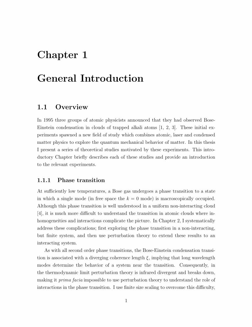
1.1.1 Phase transition
At sufficiently low temperatures, a Bose gas undergoes a phase transition to a state
in which a single mode (in free space the k = 0 mode) is macroscopically occupied.
Although this phase transition is well understood in a uniform non-interacting cloud
[4], it is much more difficult to understand the transition in atomic clouds where in-
homogeneities and interactions complicate the picture. In Chapter 2, I systematically
address these complications; first exploring the phase transition in a non-interacting,
but finite system, and then use perturbation theory to extend these results to an
interacting system.
As with all second order phase transitions, the Bose-Einstein condensation transi-
tion is associated with a diverging coherence length ξ, implying that long wavelength
modes determine the behavior of a system near the transition. Consequently, in
the thermodynamic limit perturbation theory is infrared divergent and breaks down,
making it prima facia impossible to use perturbation theory to understand the role of
interactions in the phase transition. I use finite size scaling to overcome this difficulty,
1
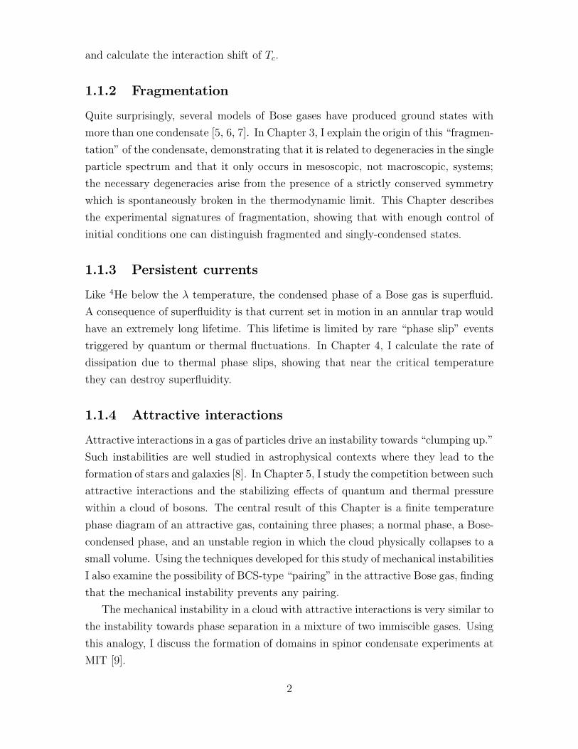
and calculate the interaction shift of Tc.
1.1.2 Fragmentation
Quite surprisingly, several models of Bose gases have produced ground states with
more than one condensate [5, 6, 7]. In Chapter 3, I explain the origin of this “fragmen-
tation” of the condensate, demonstrating that it is related to degeneracies in the single
particle spectrum and that it only occurs in mesoscopic, not macroscopic, systems;
the necessary degeneracies arise from the presence of a strictly conserved symmetry
which is spontaneously broken in the thermodynamic limit. This Chapter describes
the experimental signatures of fragmentation, showing that with enough control of
initial conditions one can distinguish fragmented and singly-condensed states.
1.1.3 Persistent currents
Like 4He below the λ temperature, the condensed phase of a Bose gas is superfluid.
A consequence of superfluidity is that current set in motion in an annular trap would
have an extremely long lifetime. This lifetime is limited by rare “phase slip” events
triggered by quantum or thermal fluctuations. In Chapter 4, I calculate the rate of
dissipation due to thermal phase slips, showing that near the critical temperature
they can destroy superfluidity.
1.1.4 Attractive interactions
Attractive interactions in a gas of particles drive an instability towards “clumping up.”
Such instabilities are well studied in astrophysical contexts where they lead to the
formation of stars and galaxies [8]. In Chapter 5, I study the competition between such
attractive interactions and the stabilizing effects of quantum and thermal pressure
within a cloud of bosons. The central result of this Chapter is a finite temperature
phase diagram of an attractive gas, containing three phases; a normal phase, a Bose-
condensed phase, and an unstable region in which the cloud physically collapses to a
small volume. Using the techniques developed for this study of mechanical instabilities
I also examine the possibility of BCS-type “pairing” in the attractive Bose gas, finding
that the mechanical instability prevents any pairing.
The mechanical instability in a cloud with attractive interactions is very similar to
the instability towards phase separation in a mixture of two immiscible gases. Using
this analogy, I discuss the formation of domains in spinor condensate experiments at
MIT [9].
2

1.1.5 Kinetic theory
In Chapter 6, I derive a kinetic theory for describing trapped alkali atoms at finite
temperature. Such a kinetic theory is needed to model non-equilibrium finite temper-
ature experiments where both quantum coherence and classical thermal fluctuations
are important. For example, one would like to understand experiments [10] where
a vortex is found to have a finite lifetime. Current theories suggest that the vortex
decays by transferring its angular momentum to the cloud of non-condensed atoms
which surround the condensate. Modeling this scenario requires a non-equilibrium
theory which simultaneously describes the coherent motion of the condensate and the
incoherent motion of non-condensed particles.
The kinetic theory derived here is quite complicated. I elucidate the essential
structure by applying this formalism to investigate a toy problem in which a uniform
gas experiences a sudden change of interaction strength. Looking at the excitations
formed during this process helps clarify the distinction between quasiparticles and
collective excitations. This distinction is unusual in a condensed gas since the con-
densate nominally hybridizes the two types of excitations.
1.1.6 Electromagnetically induced transparency
In Chapter 7, I give a detailed analysis of experiments that use a cold atomic gas
as a tunable non-linear media to control the behavior of light [11, 12]. By coupling
photons to a dark-state polarization wave, these experimentalists are able to slow
light, and even stop it. I analyze these experiments with two approaches, mean field
theory and equilibrium Green’s functions.
1.2 Experiments
Having outlined the main topics, I now give a brief review of the experiments which
have motivated this thesis. For further details I highly recommend several recent
reviews [13, 14, 15, 16], as well as an excellent elementary introduction by Carl
Wieman [17]. I limit my descriptions to the experiments referred to in the rest of this
thesis.
3

1.2.1 Cooling and trapping
Quantum mechanics limits the precision with which one can know both the position
and momentum of a particle. This restriction is encapsulated in the Heisenberg un-
certainty principle, δx · δp ≥ ~, which states that the product of the uncertainties
in position and momentum are bounded below by the constant ~ ≈ 1.054 · 10−34Js.
At finite temperature, random thermal motion leads to a large uncertainty in mo-
mentum, and consequently there is very little uncertainty in the positions of the
atoms. For example, a room temperature a sodium atom has a root mean square
velocity of 500m/s, about 1.5 times the speed of sound in air, leading to a spread,
δx ≈ 6 · 10−12m, much smaller than the size of a sodium atom. Thus room temper-
ature atoms behave as classical particles. As they are cooled to lower temperatures,
T , the atoms slow down, and the thermal wavelength λ =√
2π~2/mkBT , which
measures the uncertainty in the position of an atom of mass m, decreases. For Bose
Einstein condensation to occur, the particles must be cooled until λ is of order the
interparticle spacing (precisely, nλ3 = ζ(3/2) = 2.61 . . .). At this point the particles
lose their individual identity, and behave collectively.
The great experimental challenge of achieving Bose condensation with an atomic
vapor lies in the difficulty of cooling and compressing the vapor to the point where
nλ3 is of order unity. Liquid helium, with a number density comparable to water
n ∼ 2 · 1022cm−3 and a very low mass, Bose condenses at 2.17K. Alkali gases have
densities comparable to a good vacuum n ∼ 1012cm−3, and need to be cooled to
temperatures of order 100nK. The 1997 Nobel prize was awarded to Steven Chu,
Claude Cohen-Tannoudji, and Bill Phillips for developing laser cooling techniques,
which are necessary to cool to such unbelievably low temperatures.
Cooling is performed in several stages. The atoms, initially loaded into the appa-
ratus by boiling them off of a metallic filament, are first cooled by a series of optical
means, the most ingenious of which is the “optical molasses” consisting of six laser
beams focussed on a small point. This geometry is illustrated in Fig. 1.1. These
lasers are red detuned relative to an atomic transition. If an atom is moving towards
one of the six lasers, the light is blue-shifted into resonance and the atom absorbs a
photon. The recoil from absorbing the photon slows the atom down. This mechanism
can cool a gas to the recoil temperature, found by equating the thermal energy of an
atom with its recoil energy. For typical parameters, the recoil temperature is of order
10µK.
Further cooling relies on trapping the particles in a magnetic trap. The basic
principle is that alkali atoms, with one valence electron, have a magnetic moment
4

Figure 1.1: Schematic drawing of the laser beam configuration for an optical mo-lasses. Lasers are incident from all directions. These lasers are red-detuned relative toan atomic transition so that light will only be absorbed from a beam which is dopplershifted into residence. Consequently the atoms experience a drag which tends to slowthem down.
5

and will therefore feel a force when placed in a magnetic field gradient. A magnetic
trap consists of a set of magnets which produce a field with a local minimum at
some point in space. Atoms are trapped near this minimum. Magnetic trapping is
demonstrated by the quadrupole trap illustrated in Fig. 1.2, which simply consists of
two magnets with their north poles facing each other. The resulting magnetic field
configuration has B = 0 at the center, and |B| increasing linearly as one departs from
that point. Simple quadrupole traps are rarely used in current experiments, as these
traps are “leaky.” Atomic spins can flip where B = 0, resulting in lost atoms. Adding
an extra “Ioffe” magnet to the quadrupole configuration produces a trap where the
field does not vanish at the minimum, thus eliminating these losses. A typical Ioffe
trap is illustrated in Fig. 1.3. In such traps |B| varies quadratically as one moves from
the center, and the particles feel a harmonic potential Vtrap(r) ≈ mΩ2r2/2, where m
is the atomic mass, and Ω is the frequency of oscillation in the trap. Typically Ω is
of order 100Hz.
The trap serves two important purposes. First, it compresses the atomic cloud,
increasing the density. Second, it allows for efficient evaporative cooling. Evaporative
cooling works by removing the most energetic atoms from the cloud. Upon rether-
malizing, the gas is at a lower temperature. In the magnetic trap, the most energetic
atoms are farthest away from the center of the trap. One selectively removes these
atoms to cool the cloud. To exclusively remove these atoms, one relies upon the fact
that they experience a larger magnetic field than the other atoms, and therefore the
Zeeman splitting between different hyperfine spin states is greatest in these atoms.
By tuning a radio-frequency field to the splitting of these energetic atoms, one can se-
lectively excite them, flipping their magnetic moment and causing them to be ejected
from the trap.
When the phase space density is sufficiently large (nλ3 ≥ 2.61), quantum statis-
tical mechanics predicts that the lowest energy state in the harmonic trap will be
macroscopically occupied. In typical experiments, there are 106 atoms in this con-
densate. In the absence of interactions, the characteristic size of the condensate, L,
is set by a competition between the kinetic zero-point energy for confining the atoms
T ≈ ~2/mL2 and the trapping energy V ≈ mΩL2. For typical traps, this length is
L ≈ d =√
~/mΩ ≈ 1µm. If 106 atoms were placed in such a small space, the number
density would be 1018cm−3 (just one order of magnitude less than the density of air at
standard temperature and pressure). In practice, the repulsive interactions between
atoms restrict this density to a much lower value, and one finds L by comparing
three energies; T , V and the interaction energy U ∼ ~2Nas/mL
3. The scattering
6

Figure 1.2: Schematic drawing of a quadrupole trap. Two magnets with their polesfacing each other create a quadrupolar field in the region between them. The smallovoid represents an atomic cloud trapped at the minimum of the magnetic field.
7

Figure 1.3: Ioffe-Pritchard trap, as used in current BEC experiments. All linesrepresent wires carrying electric currents in the directions indicated by the arrows.The Ioffe bars create an in-plane quadrupole field. The pinch coils turn this into a3D quadrupole field, and the bias coils (or compensation coils) generate a non-zeromagnetic field at the center of the trap.
8

length as parameterizes the interactions1 and, with a few notable exceptions, as is
positive and of order 5 nm, implying that U ≫ T , and that the size of the condensate
is determined by a competition between U and V . Comparing these energies gives
L ≈ (Nas/m2Ω2)1/5 which is of order 10µm, resulting in a density n ∼ 1013cm−3
[18]. This density is much greater than the density of atoms above the condensation
temperature n = 1011cm−3, and the phase transition therefore coincides with the
appearance of a large spike in the density of atoms at the center of the trap. An
example of the experimental density profile is shown in Fig. 1.4. The density spike is
clearly visible at temperatures below Tc.
Figure 1.4: Density profile of trapped atoms above and below Tc, reproduced withpermission from the MIT group’s web site http://cua.mit.edu/ketterle_group/
Projects_1995/Three_peaks/3peaks%20gray1.jpg. These pictures are absorptionimages of the cloud after ∼ 100ms of free expansion, the height representing theoptical depth (see Section 1.2.2).
1.2.2 Measurement procedures
In order to interpret the experimental data, one needs to understand the principle
techniques used to probe atomic clouds. These techniques have enabled experimental-
ists to produce pictures which beautifully illustrate the quantum mechanical nature
of atoms. All of the methods that I discuss can be used in two ways; either as in
situ measurements, in which the trapped atoms are directly probed, or as expansion
measurements, in which the trap is turned off and the cloud expands before the mea-
surement is made. The main advantage of in situ measurements is that one directly
measures the properties of the trapped gas. However, due to the small size of the
1For a detailed discussion of atomic scattering, see appendix F
9
AtomicCloud
Laser
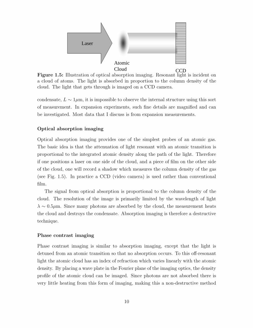
CCDFigure 1.5: Illustration of optical absorption imaging. Resonant light is incident ona cloud of atoms. The light is absorbed in proportion to the column density of thecloud. The light that gets through is imaged on a CCD camera.
condensate, L ∼ 1µm, it is impossible to observe the internal structure using this sort
of measurement. In expansion experiments, such fine details are magnified and can
be investigated. Most data that I discuss is from expansion measurements.
Optical absorption imaging
Optical absorption imaging provides one of the simplest probes of an atomic gas.
The basic idea is that the attenuation of light resonant with an atomic transition is
proportional to the integrated atomic density along the path of the light. Therefore
if one positions a laser on one side of the cloud, and a piece of film on the other side
of the cloud, one will record a shadow which measures the column density of the gas
(see Fig. 1.5). In practice a CCD (video camera) is used rather than conventional
film.
The signal from optical absorption is proportional to the column density of the
cloud. The resolution of the image is primarily limited by the wavelength of light
λ ∼ 0.5µm. Since many photons are absorbed by the cloud, the measurement heats
the cloud and destroys the condensate. Absorption imaging is therefore a destructive
technique.
Phase contrast imaging
Phase contrast imaging is similar to absorption imaging, except that the light is
detuned from an atomic transition so that no absorption occurs. To this off-resonant
light the atomic cloud has an index of refraction which varies linearly with the atomic
density. By placing a wave plate in the Fourier plane of the imaging optics, the density
profile of the atomic cloud can be imaged. Since photons are not absorbed there is
very little heating from this form of imaging, making this a non-destructive method
10

suitable for making “movies” of a single cloud.
RF spectroscopy
As an alternative to imaging the cloud, one can use spectroscopic probes to study an
atomic gas. One spectroscopic approach, currently restricted to hydrogen experiments
[19], takes advantage of the pressure shift of an atomic transition. The 1s-2s two-
photon transition in hydrogen is red shifted under increased pressure. The microscopic
basis for this shift is that atoms in the 2s state interact less strongly with 1s atoms
than 1s atoms interact with themselves. Thus the energy of the 2s state relative to the
1s state is reduced as the atomic density in increased. By measuring the frequency of
the 1s-2s transition one can determine the density of a uniform atomic cloud. More
importantly, in an inhomogeneous cloud, the 1s-2s line will be broadened, the line
shape giving a histogram of the density of the cloud.
Atom detection
Experiments on gases of excited He atoms have made use of yet another measurement
scheme. Ground state He atoms cannot be magnetically trapped as they do not have
a magnetic moment. Using a long lived excited state, two groups of experimentalists
have successfully trapped a gas He atoms, and cooled them below the BEC transition
temperature [20, 21]. In the latter experiment [21], the system is probed by releasing
the atoms from the atomic trap and letting them fall onto a microchannel plate. At
the plate, the excited atoms drop into their ground state, each releasing an easily
measurable 20 eV of energy. A plot of the signal voltage versus time gives the density
profile of the cloud.
1.2.3 Fermions
Alkali gas experiments are performed with both bosonic and fermionic isotopes. Most
of this thesis is concerned with bosonic atoms, but experiments on fermions are quite
exciting [22] and much of the material in Chapters 5 and 6 is readily extended to
include fermions. Quantum degeneracy does not correspond to a phase transition
in a Fermi gas, just a cross-over from classical behavior to quantum behavior as
the Fermi surface becomes sharper. Fermionic atoms are cooled and imaged in the
same manner as bosons, with the caveat that evaporative cooling works poorly. The
problem is that in evaporative cooling, after the most energetic atoms are removed,
the remaining atoms must thermalize. As a Fermi surface develops the phase space
11

available for collisions becomes small, and the thermalization time becomes very long.
This difficulty is compounded by the absence of s-wave collisions between identical
fermions in the same spin state. These collisions are forbidden because the Fermi
wavefunction is antisymmetric.
To help circumvent these problems, some fermion experiments rely upon sympa-
thetic cooling, where a mixture of Fermi and Bose atoms are loaded into the magnetic
trap. The Bose atoms are easier to cool, and can be used as a buffer gas which absorbs
the heat from the fermions. In this manner temperatures as low as one third of the
Fermi temperature have been achieved. A major goal of these fermion experiments
is to achieve BCS pairing in a gas of alkali atoms.
1.2.4 Coherence experiments
A Bose condensate is to a normal gas as a laser is to a thermal light source. A
condensate has a high degree of coherence. This coherence can be seen in various
sorts of interference experiments. The simplest of these is an analogy of a double-slit
experiment [23], in which investigators create an atomic trap with two distinct minima
and an insurmountable barrier between them. They cool a cloud in this double-well
trap, forming two condensates. When the trap is turned off, the clouds expand and
overlap, as sketched in Fig. 1.6. Absorption images, reproduced in Fig. 1.7, revealed
a distinct interference pattern, reminiscent of the pattern seen in a classic two-slit
diffraction experiment. This interference pattern shows a form of coherence, and
would not occur in a non-condensed gas.
This experiment raises some very subtle issues. Suppose the two clouds were
formed completely independently. Bose condensation implies that there should be
coherence between any two points in the same cloud, such that if you split one of the
clouds it would interfere with itself. It is not clear, however, that the two independent
clouds would interfere with each other. A detailed analysis of why interference is seen
will be given in Section 3.2.2 (page 46).
1.2.5 Collapse of an attractive gas
Although most alkali atoms interact with repulsive interactions, there exist several
atoms with attractive interactions, most notably 7Li and 85Rb [24, 25]. A Bose gas
with attractive interactions is unstable towards a mechanical collapse. At zero tem-
perature stability can be understood through a simple dimensional argument where
one explores how the energy of a cloud varies as one changes the size of the system L.
12

a)
b)
c)
Figure 1.6: Diagram to illustrate an atom wave interference experiment. a) Twocondensates are created in a double-well trap. b) The trap is turned off and the cloudsexpand. c) The overlapping clouds interfere with one another to form a modulateddensity pattern.
13

Figure 1.7: Absorption image from an experiment where two atomic condensates areallowed to overlap and interfere. Darker colors correspond to larger column densities.Data reproduced from [23].
14
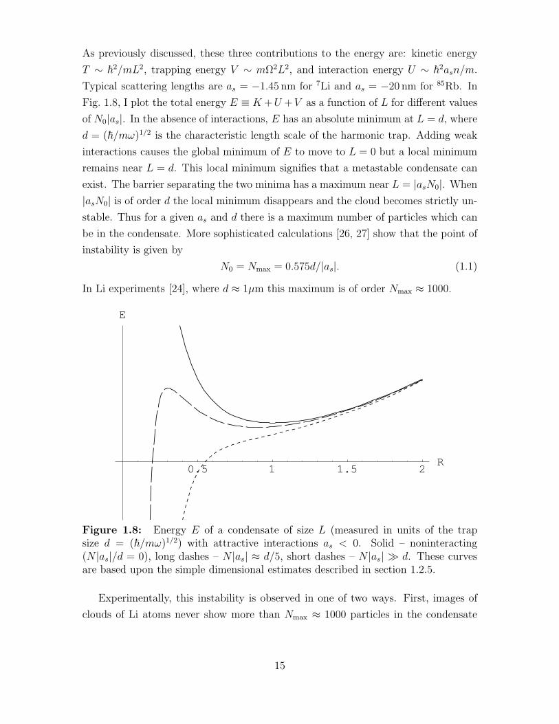
As previously discussed, these three contributions to the energy are: kinetic energy
T ∼ ~2/mL2, trapping energy V ∼ mΩ2L2, and interaction energy U ∼ ~
2asn/m.
Typical scattering lengths are as = −1.45 nm for 7Li and as = −20 nm for 85Rb. In
Fig. 1.8, I plot the total energy E ≡ K+U +V as a function of L for different values
of N0|as|. In the absence of interactions, E has an absolute minimum at L = d, where
d = (~/mω)1/2 is the characteristic length scale of the harmonic trap. Adding weak
interactions causes the global minimum of E to move to L = 0 but a local minimum
remains near L = d. This local minimum signifies that a metastable condensate can
exist. The barrier separating the two minima has a maximum near L = |asN0|. When
|asN0| is of order d the local minimum disappears and the cloud becomes strictly un-
stable. Thus for a given as and d there is a maximum number of particles which can
be in the condensate. More sophisticated calculations [26, 27] show that the point of
instability is given by
N0 = Nmax = 0.575d/|as|. (1.1)
In Li experiments [24], where d ≈ 1µm this maximum is of order Nmax ≈ 1000.
0.5 1 1.5 2R
E
Figure 1.8: Energy E of a condensate of size L (measured in units of the trapsize d = (~/mω)1/2) with attractive interactions as < 0. Solid – noninteracting(N |as|/d = 0), long dashes – N |as| ≈ d/5, short dashes – N |as| ≫ d. These curvesare based upon the simple dimensional estimates described in section 1.2.5.
Experimentally, this instability is observed in one of two ways. First, images of
clouds of Li atoms never show more than Nmax ≈ 1000 particles in the condensate
15

[24]. Second, by using Feshbach resonances,2 the scattering length as of 85Rb atoms
can be tuned from positive to negative. With as > 0, a stable condensate is formed.
The scattering length is then gradually reduced until collapse occurs [25], and one
finds, as expected, that Nmax ∝ 1/|as|.
1.2.6 Spin relaxation
A very rich class of phenomena involve the hyperfine spin of a gas of alkali atoms.
The spin degree of freedom is frozen in magnetic traps, but can be accessed in optical
traps. In Section 5.6 I give a theoretical explanation of one experiment on spinor
condensates [9]. In this experiment a spinor cloud with ferromagnetic interactions is
placed in a state in which the magnetization is everywhere zero. This is an excited
state of the system and it relaxes to a state which is locally magnetized. Since
magnetization is conserved during the dynamics, a domain structure is formed where
each region is polarized in a different direction. In Section 5.6 I only discuss the
stability of the initial state. The formalism of Chapter 6 can be used to describe the
actual dynamics of the domain formation.
1.2.7 Electromagnetically induced transparency
In experiments at Rowland Institute [11] and at Harvard [12], experimentalists have
used a cold atomic gas as a nonlinear media to manipulate light. Their most striking
achievements have involved actually freezing a beam of light for several milliseconds.
I discuss the theory in Chapter 7. The basic idea is that light couples polarization
waves in an atomic gas. The small velocities of these polarization waves are inherited
by the hybridized excitations, and the light therefore propagates very slowly through
the media. Stopping the light involves adiabatically transforming the photons into
polarons, then reversing the process several milliseconds later.
1.2.8 Feshbach resonance
In recent experiments, experimentalists demonstrated the ability to tune the interac-
tion strength of a dilute gas [28]. This technique is used to explore the collapse of
attractive gases (see section 1.2.5). The interactions are controlled by using magnetic
fields to adjust the energy of a scattering resonance, bringing it near threshold. Scat-
2Feshbach resonances are magnetically induced scattering resonances, and are discussed in ap-
pendix F on page 183
16

tering resonances are discussed in detail in appendix F, where the general theory of
atomic scattering is reviewed.
It would be extremely exciting to use this technique to study the highly correlated
state of matter that would be formed when the interactions are made very strong.
In particular one could study a regime where there is a distinct separation of length
scales, with the scattering length as much larger than the interparticle spacing n−1/3,
which in turn is much larger than the physical size of the atom. In such a limit one
expects both the scattering length and the size of the atom to drop out of the problem,
and a gas of such atoms should behave in some universal manor. Experiments in this
regime have been hampered by large inelastic losses which are not fully understood.
17
Chapter 2
Theory of the BEC Phase
Transition
The dominant feature in the thermodynamics of cold Bose gases is the presence of
a phase transition to a Bose condensed state where a single-particle level is macro-
scopically occupied. Although Bose-Einstein condensation was predicted in 1925 [29],
some aspects of the phase transition have only recently been understood. In partic-
ular, it was not until the path integral Monte-Carlo calculations of Gruter, Ceperley
and Laloe [30] that the influence of interactions on the phase transition of a uniform
Bose gas was systematically explored.1 Their results, plotted in Fig. 2.1, show that
for small interaction strength the critical temperature increases with interactions,
while for larger interactions the opposite behavior occurs. The drop in Tc can be
qualitatively understood as an effective mass effect. An atom moving through the
fluid must drag other atoms with it, giving it a larger effective mass. Since Tc ∝ m−1,
the critical temperature is reduced.
The weakly interacting case has only recently been understood analytically [32,
33]. An intuitive argument is that repulsive interactions reduce density fluctuations
and therefore increase the occupation of the k = 0 mode, raising Tc. Quantifying this
argument is difficult, and the calculations of Tc [32, 33] rely upon very mathematical
arguments whose physical interpretations are not directly evident.
Here I use a novel approach to calculating the change in Tc, based upon pertur-
bation theory in powers of the interaction. One cannot directly use perturbation
theory to calculate Tc since the perturbation series suffers from infrared divergences
1As the phase transition temperature is of fundamental importance, many earlier works discussed
this topic [31], but the first systematic and authoritative review of the subject was due to Gruter,
Ceperley, and Laloe.
18

PSfragreplacements0:01
0:1 1:0
1:0 1:0
0:020:03
0:40:60:8
1:081:061:041:02
106 105 104 103 0:01
T C=T 0T C=T 0
na3
simulation results4He (a3n)0:34freezing at T = 0 &
Figure 2.1: Change of Critical temperature with interaction strength, reproducedwith permission from [30]. For na3 < 0.01 the transition temperature increaseswith interaction strength, while for larger na3 the opposite occurs. The apparentdiscontinuity of the slope at na3 ≈ 0.1 is an artifact of using a different scale for∆T > 0 and ∆T < 0. The dashed line is a power-law fit to the small na3 data,and the dotted line is a guide to the eye. In this chapter I discuss the regime wherena3 ≪ 1.
19

at the critical point. These divergences are a common feature of second order phase
transitions where long wavelength properties dominate the behavior of the system.
I avoid these singularities by working in small systems where the finite system size
provides a low energy cutoff. Studying the scaling properties of these small systems
reveals the phase transition temperature.
Although this discussion of the phase transition of a uniform system is of extreme
fundamental importance, it is not particularly relevant to experiments on trapped
atoms. In a harmonic trap the dominant shift in the transition temperature is due to
the way in which interactions change the shape of the cloud. This shift is describable
within mean field theory, and has been experimentally verified [34].
This Chapter is organized as follows. First I review the elementary text-book level
description of Bose-Einstein condensation. Next I look at finite size effects, and inves-
tigate scaling in small systems. I then combine these results with perturbation theory
to calculate the first order shift in the critical temperature ∆T . Finally I give a brief
calculation of the shift in a harmonically trapped cloud. The work presented in this
Chapter was performed in collaboration with Gordon Baym and Markus Holzmann,
and has been accepted for publication [35].
2.1 Elementary description
To preface my discussion of the phase transition, I give an elementary review of Bose
condensation in an ideal gas [4] in the grand canonical ensemble. I begin by consider-
ing a cloud of non-interacting Bosons in an external potential. Special consideration is
given to the case where the particles are in a box of volume V with periodic boundary
conditions, and the case of a harmonic trap.
All thermodynamic quantities are determined by the grand free energy F , defined
in terms of the grand partition function,
Z = e−βF = Tr e−β(H−µN), (2.1)
where β = 1/kBT , H is the Hamiltonian operator, µ is the chemical potential, N
is the number operator, and the trace is taken over all possible states of the system
with any possible number of particles. I will use units where Boltzmann’s constant
kB, is equal to unity. As we are dealing with non-interacting particles, the states are
defined by occupation numbers ni, corresponding to the single particle energy levels
20
εi. The trace is explicitly written as
Z =∑
nie−β
P
i(ǫi−µ)ni , (2.2a)
=∏
i
1
1 − e−β(ǫi−µ), (2.2b)
which implies that the free energy has the form
F = −T∑
i
log(
1 − e−β(εi−µ))
. (2.3)
To extract the structure of this free energy, I introduce the density of states
ρ(E) =∑
i
δ(E − εi). (2.4)
Near the phase transition, infrared modes dominate the sum (2.3). Looking at this
low energy sector of Eq. (2.3), one can approximate log(1−e−β(E−µ)) ≈ log(βE−βµ),
yielding a free energy
F ≈ T
∫ Ec
0
dE ρ(E) [log(βE) + log(1 − µ/E)] . (2.5)
The cutoff, Ec, eliminates the high energy modes which are not correctly accounted
for by this approximation. In the exact expression (2.3), the temperature plays the
role of this cutoff;, thus Ec should be of order kBT . The phase transition occurs at
µ = 0, where either F , or one of its derivatives is singular. Assuming a power law
density states, ρ(E) ∼ Eα as E → 0, the k’th derivative ∂kF/∂µk is singular for all
k ≥ α. Since N = ∂F/∂µ, there exists a phase transition at finite density if and only
if α > 1.
For example, particles in d-dimensional free space have a power-law density of
states satisfying α = d/2− 1, and Bose condensation occurs in all dimensions greater
than 2. For harmonically trapped particles, α = d− 1, and Bose condensation occurs
in all dimensions greater than 1. In the following two subsections I explicitly calculate
the transition temperature in each of these examples.
2.1.1 Uniform gas
Most elementary textbooks, e.g. [4], describe the Bose condensation transition of
particles in a box of size L with periodic boundary conditions, where the single-
particles energies are ε = (2π2~
2/mL2)(n2x + n2
y + n2z), with nν = 0,±1,±2, . . ., and
21

m is the particle mass. To calculate the free energy it is convenient to expand the
logarithm in (2.3) and write the free energy as
F = T
∞∑
j=1
1
j
∑
i
e−βj(εi−µ). (2.6)
Ignoring the discrete nature of the spectrum at hand, one finds
F = −T∑
j
zj
j
(∫
dn e−βj
“
2π2~2
mL2
”
n2
)3
, (2.7a)
= −T Vλ3
∑
j
zj
j5/2. (2.7b)
Here I have introduced the fugacity z = eβµ and the thermal wavelength λ =
(2π~2β/m)
1/2. The series gν(z) =
∑
j zj/jν is known as either a “Bose” function,
or a polylogarithm. The latter name reflects the fact that g1(z) = − log(1 − z).
These functions are discussed at length in Appendix A.1. Replacing the sum over n
with an integral is equivalent to replacing the discrete density of states with a smooth
function ρ(E) ∝ E1/2.
To calculate the number of particles one differentiates (2.7b) to find
N = −∂F∂µ
=V
λ3g3/2(z), (2.8)
which is bounded above by Nc = V/λ3ζ(3/2), where ζ(3/2) = g3/2(1) ≈ 2.61 . . . is
the Riemann zeta function. Thus this semiclassical approximation is incapable of
describing a Bose gas at a temperature below
Tc =2π
mkB
(
n
ζ(3/2)
)2/3
. (2.9)
This approximation breaks down because the lowest energy state becomes macro-
scopically occupied below Tc. By removing this one state from the integral one avoids
this problem, finding
F = T log(1 − z) − TV
λ3
∑
j
zj
j5/2. (2.10)
Unless |βµ| < λ3/V , the first term in negligible compared to the latter. Within this
extended theory,
N =z
1 − z+V
λ3g3/2(z). (2.11)
22

We now take the thermodynamic limit N → ∞, and V → ∞, with n = N/V fixed.
If n < ζ(3/2)/λ3 the thermodynamic limit is reached at fixed z, and the density is
given by Eq. (2.8). If n > ζ(3/2)/λ3, one must scale z with the system volume such
that βµ ∼ V −1 as V → ∞, giving for T < Tc,
n = n0 + ζ(3/2)/λ3, (2.12)
where n0 = N0/V = (−βµV )−1 is the density of condensed particles.
2.1.2 Harmonically trapped gas
As discussed in Section 1.2, in recent experiments the particles are trapped in har-
monic potentials V (r) = mΩ2r2/2. The energy levels in a harmonic trap are of the
form εi = ~Ω(nx + ny + nz + 3/2), where nν = 0, 1, 2, . . .. The zero point energy
(3/2)~Ω plays no role in the following arguments and I will neglect it. The free en-
ergy of the harmonically trapped gas has the same structure as the gas in free space,
and I jump to the equivalent of Eq. (2.10),
F = T log(1 − z) − T∑
j
zj
j
(∫ ∞
0
dn e−β~Ωnj
)3
, (2.13a)
= T log(1 − z) − T
(β~Ω)3
∑
j
zj
j4, (2.13b)
giving a mean number of particles,
N =z
1 − z+
1
(β~Ω)3g3(z). (2.14)
In the trap, the thermodynamic limit is approached by letting N → ∞ and Ω → 0
such that Ω3N is constant, which keeps constant the density at the center of the
trap. As in the analysis of Eq. (2.11), at fixed z the number of particles is bounded
by N ≤ ζ(3)/(β~Ω)3, equality representing the Bose-Einstein condensation phase
transition. If one treats the µ→ 0 limit in a similar fashion to Section 2.1.1 one finds
for T < Tc,
N = N0 +ζ(3)
(β~Ω)3. (2.15)
2.2 Finite size effects
Although statistical mechanics tells us that there are no phase transitions in finite
systems, we apparently see phase transitions all around us. Conventionally, this con-
tradiction is resolved by stating that the finite system possesses a crossover between
23

two distinct behaviors. As the system size increases, the crossover becomes sharper
and mimics a phase transition.
A rather sophisticated understanding of finite size effects comes from studying the
renormalization group [36]. In these studies, one imagines an abstract space param-
eterized by all the possible couplings which could exist in the model being studied
– for instance temperature, interaction strength, and system size. The renormaliza-
tion group (RG) is a mapping of this space onto itself where each model is coarse
grained and reduced in scale. Under this mapping, systems will flow to various fixed
points. Each stable fixed point represents a different phase of matter. Critical points
are associated with unstable fixed points – the system flows in different directions
depending upon which side of the critical point it starts on. A schematic depiction
of the RG flow for a Bose gas is portrayed in Fig. 2.2, where two of the couplings,
the temperature and the system size, are shown. Two fixed points are depicted, the
critical fixed point and a low temperature fixed point corresponding the the Bose
condensed phase. A few sample flow lines are drawn as well as two regions, a critical
region and a finite size scaling region, both of which are discussed below.
In this thesis I do not calculate any RG flows, however I will use one of the
generic results; namely that if a system is in the critical region near a fixed point, its
behavior is dominated by that fixed point, and physical quantities obey a set of scaling
relationships. In particular, the finite size scaling hypothesis holds. This hypothesis
states that all physical quantities scale as functions of the ratio of the correlation
length ξ to the system size L. The correlation length ξ is a measure of the fall off of
the two-point function 〈ψ†(r)ψ(0)〉, and diverges at the critical point. An example of
this scaling is the prediction that the number of condensed particles should scale as
〈N0〉V
∼ L−yΦ(L/ξ), (2.16)
where y = β/ν = 1 is the ratio of the critical exponents for N0/V and the correlation
length, and Φ is a scaling function. As L/ξ → ∞, this function must diverge as
Φ(L/ξ) ∼ (L/ξ)y, while as L/ξ → 0, Φ approaches a constant. The region where
L << ξ is the finite size scaling regime, and the scaling law (2.16) can be used to
systematically find the critical point (ξ → ∞) by looking solely at the properties of
a finite system.
As an example of using Eq. (2.16) to find the critical point, consider the numerical
calculations of Gruter et al. [30] discussed in the introduction of this Chapter. In that
calculation, the authors used a Monte-Carlo technique to find the superfluid density
ρs (which on dimensional grounds scales as N0/V ) as a function of temperature and
24

Figure 2.2: Schematic renormalization group flow diagram for a Bose gas. Pointson this graph represent Bose gases of a given temperature T and system size L.The dashed arrows show how a system changes under the renormalization group – acoarse graining and rescaling procedure. Two fixed points of this operation are shownas large dots; the critical point and the BEC fixed point. A critical regime, wherephysical quantities obey power law scaling relationships is shown. Also depicted is thefinite-size scaling regime where the coherence length is large compared to the systemsize, ξ ≫ L. In this regime the finite size scaling laws apply.
system size for various small systems. Curves of Lyρs as a function of temperature
for different L all crossed at a temperature T∗. According to Eq. (2.16) this is the
temperature at which the coherence length diverges, which is by definition the critical
temperature.
In the following sections I use elementary means to explicitly verify the scaling
relation (2.16) for the non-interacting gas. I then use this relationship to calculate
the phase transition temperature of an interacting gas.
2.2.1 Scaling in the ideal gas
Here I identify the BEC phase transition in a non-interacting gas from the scaling
of the number of condensed particles. This simple example illustrates the technique
which I use to calculate Tc for the interacting system. I first perform this calculation in
the grand canonical ensemble, and then in the canonical ensemble. In the presence of
a condensate the thermodynamics of an ideal gas are sensitive to the ensemble used.
This sensitivity is demonstrated by looking at the distribution function P (N0) for
the number of condensed particles. Within the grand canonical ensemble, P (N0) ∝
25

e−β(ε0−µ)N0 , is exponentially decaying at all temperatures. On the other hand, at zero
temperature in the canonical ensemble, P (N0) = δN,N0 is a delta function, as all of
the particles are in the condensate. Thus P (N0), a macroscopic observable, behaves
qualitatively differently depending on the ensemble. Any observable which depends
on fluctuations in the number of condensed particles (like the compressibility) will
likewise be sensitive to the ensemble.
Despite these differences, the phase transition temperature is expected to be in-
dependent of the ensemble. It turns out that it is easier to perturbatively calculate
∆T within the canonical ensemble than within the grand canonical ensemble.
Grand canonical results
Here I calculate the phase transition temperature of the ideal gas within the grand
canonical ensemble. My general strategy is to fix the average density n = N/V and
the temperature T , and look at how the number of condensed particles N0 varies
with the system size L. To carry out this approach one needs an expression for the
chemical potential µ as a function of n, T , and L; requiring that one inverts Eq.
(2.11). The inversion is performed by expanding (2.11) in powers of βµ. Using the
expansion of the polylogarithm given in Appendix A.1, one finds
n =1
λ3
[
ζ(3/2) +λ
L
(
− 1
βµL2/λ2− 2√
−πβµL2/λ2
)
+ · · ·]
; (2.17)
the neglected terms are of higher order in βµ, and are negligible near the transi-
tion temperature as long as N ≫ 1. The terms proportional to 1/βµ and√−βµ
are respectively the contributions from the condensed and non-condensed particles.
Finding βµ as a function of n, T , and L, requires solving a cubic equation. I define
the function F (x), plotted in Fig. 2.3, as the solution to
1
F (x)− 2√
πF (x) − x = 0, (2.18)
so that the chemical potential can be expressed as,
βµ = −λ2
L2F
(
L
λ
(
λ3n− ζ(3/2))
)
. (2.19)
The positive, monotonic F (x) has the properties
F (0) = (4π)−1/3 (2.20)
F (x) −→x→−∞
x2/4π (2.21)
F (x) −→x→+∞
1/x. (2.22)
26

Thus, as L→ ∞, the order parameter N0 ≈ −1/βµ, has three distinct behaviors, cor-
responding to non-condensed, critical, and condensed regimes, depending on whether
n is less than, equal to, or greater than ζ(3/2)/λ3. In the non-condensed regime, N0 is
microscopic, in the condensed regime, N0 is extensive, and at the critical temperature,
N0 scales as L2, i.e.,
n < ζ(3/2)/λ3, N0 ∼ L0 (2.23)
n = ζ(3/2)/λ3, N0 ∼ L2 (2.24)
n > ζ(3/2)/λ3, N0 ∼ L3. (2.25)
-5 5 10 15 20x
1
2
3
4
5FHxL
Figure 2.3: The function F (x), defined as the solution to Eq. (2.18), which relatesthe chemical potential and density of a non-interacting Bose gas via Eq. (2.19). Theasymptotic expressions (2.21) and (2.22) are plotted as dashed lines.
This scaling behavior is illustrated by Fig. 2.4, which shows the condensate fraction
N0/N as a function of N for different values of the reduced temperature t = T/Tc.
The various power laws can be read directly from the graph. Note that for small N ,
the critical regime where N0 ∼ N2/3 has a finite width. This width is estimated by
linearizing the chemical potential (2.19) about the point n = ζ(3/2)/λ3 to find
N0 =L2
λ2(4π)1/3 +
L3
λ3
2
3
(
λ3n− ζ(3/2))
+L2
λ2O(
L
λ(λ3n− ζ(3/2))
)2
. (2.26)
27

The number of condensed particles scales as L2 over a temperature range δT/Tc ≈λ/L, and then crosses over to the asymptotic behavior described in Eqs. (2.23) and
(2.25).
102 104 106 108 1010N
10-8
10-6
10-4
10-2
100
N0N
t=0
t=0.9
t=0.99
t=1
t=1.01
t=1.1
t=2
Figure 2.4: Condensate fraction N0/N versus N for various values of the reducedtemperature t = T/Tc. The three scaling regimes for t < 1, t = 1, and t > 1,correspond to the condensed, critical, and non-condensed regimes, in which N0 ∼ N ,N0 ∼ N2/3, and N0 ∼ N0.
2.2.2 Scaling in the canonical ensemble
I now repeat the calculation of Section (2.2.1) in the canonical ensemble. As previ-
ously mentioned, in the presence of the condensate, thermodynamic properties of an
ideal Bose gas are sensitive to the ensemble used.
In this section I look at scaling in P (N0) rather than just at N0, as was done
in Section (2.2.1). Generalizing Eq. (2.16), one expects that at Tc the probability
distribution function can be written as
P (N0) =λ2
L2ψ(N0λ
2/L2), (2.27)
with some scaling function ψ. As I demonstrate here, this relationship holds for the
non-interacting gas.
28
The canonical distribution function can be expressed as
P (N0) =1
ZNTr
N,N0 fixede−βH =
1
ZNe−βF (N,N0), (2.28)
where the trace is taken at fixed N and N0, and β is the inverse temperature. This
equation defines the free energy F (N,N0), and uses the partition function, ZN =∑
N0e−βF (N,N0), to normalize the probability distribution. In the non-interacting gas,
F (N,N0) is only a function of Nex = N −N0 and is identifiable as the free energy of
the non-condensed particles,
F (N,N0) = Fex(Nex). (2.29)
Although the condensate’s behavior depends crucially on the ensemble, one expects
that the properties of the non-condensed particles will be insensitive to the ensemble,
and one should be able to calculate Fex via a Legendre transformation of the grand
free energy,
Fex(Nex) = Fex(µ(Nex)) + µ(Nex)Nex, (2.30)
where µ(Nex) = ∂Fex/∂Nex is a chemical potential which represents the free-energy
cost of exchanging particles between the condensate and the non-condensed particles.
Intuitively, the condensate acts as a particle bath for the non-condensed system. The
chemical potential varies with Nex since as one depletes the condensate the cost of
removing particles from the condensate changes.
As in Section 2.2.1, I need to relate Nex and µ. The approximation of Eq. (2.17)
is not sufficient, since I will need to take the limit µ → 0. The relevant asymptotics
are evaluated in Appendix B, where according to Eq. (B.13), µ and Nex are related
by
Nex = f1 =
(
L
λ
)3
ζ(3/2) +
(
L
λ
)2
h
(
βµL2
λ2
)
+ O(L/λ), (2.31)
h(x) =∞∑
k=0
xk
k!C3(k + 1). (2.32)
The coefficients C3(k + 1) are tabulated in Table. B.1. Inverting the series, and
replacing Nex with N −N0 gives
βµ =λ2
L2
(
− 1
C3(2)M − C3(3)
2(C3(2))2M2 + · · ·
)
, (2.33)
M = N0λ2
L2+ C3(1) − λ2
L2
(
N − L3
λ3ζ(3/2)
)
, (2.34)
29
from which the free energy is
βF (N,N0) = −∫
dN0 (βµ) (2.35)
= βF (N) +1
2C3(2)M2 +
C3(3)
6(C3(2))2M3 + · · · (2.36)
≡ βF (N) + g(M), (2.37)
where F (N) is an extensive function which is independent of N0, and g(M) is defined
by Eqs. (2.36,2.37). If n = N/V = ζ(3/2)/λ3, then M depends on L only through
the variable N0λ2/L2, implying that P (N0) is of the form
P (N0) =λ2
L2ψ(N0λ
2/L2), (2.38)
where the scaling function ψ is found by exponentiating (2.35). For any other value
of the density, M has additional L dependence, and P (N0) does not scale like (2.38),
implying that the scaling holds only at Tc. In Fig. 2.5 I plot P (N0) at the critical
point. The Gaussian approximation, where only the term proportional to M2 is kept,
is also plotted, and agrees quite well with the full result.
1 2 3 4 5 6 7 N0Λ2L2
0.05
0.1
0.15
0.2
0.25
0.3
L2Λ2
PHN0L
Figure 2.5: Probability distribution P (N0) for the number of condensed particles atthe critical temperature in a non-interacting Bose gas within the canonical ensemble.Dashed line is a Gaussian approximation. At the critical point, P has the scalingform (2.38).
30

2.3 Perturbative calculation of ∆T .
In this section I use first order perturbation theory to calculate the critical temper-
ature of a weakly interacting Bose gas. In Section 2.3.1 I present the structure of
perturbation theory, demonstrating that due to infrared divergences it breaks down
in the thermodynamic limit. In Section 2.3.2 I use the techniques of Section 2.2.2 to
circumvent these difficulties and calculate the transition temperature.
Here I work in the canonical ensemble. Within the grand canonical ensemble, first
order perturbation theory changes the energy of each momentum state by the same
amount. This shift can therefore be absorbed into the chemical potential, leaving the
transition temperature unchanged. The first effects start at higher order; exploring
how higher order perturbation theory in conjunction with finite size scaling can be
used to calculate the shift of Tc in the grand canonical ensemble is beyond the scope
of this thesis.
2.3.1 Perturbation theory
A cloud of bosons that interact through a short range potential is described by a
Hamiltonian
H =∑
q
~2q2
2mb†qbq +Hint, (2.39)
where
Hint =2π~
2as
mV
∑
pkq
b†pb†qbq−kbp+k, (2.40)
and as is the scattering length, bq is the annihilation operator for particles with
momentum q, m is the particle mass, and V ≡ L3 is the volume of the system.
As in Section 2.2.2, the function of interest is the probability distribution for the
number of condensed atoms. P (N0) ∝ e−βF (N,N0). Expanding F (N,N0) to first order
in the interaction,
F (N,N0) = F0(N,N0) + 〈Hint〉N,N0, (2.41)
where the expectation value is in the free ensemble, and F0 ≡ F (a = 0) is the free
energy of the non-interacting system.
It is straightforward to calculate 〈Hint〉 using the approximation of Section 2.2.2.
The expectation value involves the sum
∑
pqk
〈b†pb†qbq−kbp+k〉 = 2N2 −∑
p
〈Np(Np + 1)〉, (2.42)
31

where Np = b†pbp. Using the assumption that for a fixed N0 the non-condensed
particles are grand-canonically distributed,
∑
p
〈Np(Np + 1)〉 = N0(N0 + 1) +∂Nex
∂µex
. (2.43)
At Tc, each of these terms scale as (L/λ)4. The first order correction to F (N,N0)
therefore scales as
∆F (N,N0) ∼ kBT asL/λ2 ≡ kBT η, (2.44)
which defines η. Higher order terms in the expansion of the free energy involve addi-
tional powers of βHint. Successive terms are of relative size 〈(βHint)m〉/〈(βHint)
m−1〉 ∼η. Thus the perturbation expansion is valid only for sufficiently small η. Since η in-
volves the product as × L, the limits as → 0 and L→ ∞ are not interchangeable.
2.3.2 Calculation of ∆T
Here I calculate ∆T , the interaction induced change in Tc. My strategy is to find the
temperature at which the first order expression (2.41) has the scaling form (2.27).
This temperature should be close to the transition temperature of the ideal gas T(0)c ,
so I write, T = T(0)c + ∆T , and expand to first order in ∆T . The resulting expression
is
βF (N,N0, T ) = βF0(T(0)c ) + ∆T
∂F0
∂T+ ∆F (T 0
c ), (2.45)
where for clarity I have omitted the arguments N and N0 on the right hand side. The
first order correction ∆F is given in Eq. (2.41). If one substitutes Eq. (2.36) for F0,
this free energy can be expressed as
βF (N,N0, T ) = βF0 + g(M0) −∆T
T
λ2
L2N0g
′(M0) (2.46)
+3
2
∆T
T
L
λζ(3/2)g′(M0) −
2π~2as
mV T
(
N20 + 2
∑
k 6=0
Nk(Nk + 1)
)
,
where the argument M0 = N0(λ2/L2) + C3(1) is the scaled condensate number mea-
sured from the peak of the distribution. The first two terms are the free energy of
the non-interacting gas at T(0)c , while the remaining terms give the first order correc-
tions in ∆T and as. These corrections are only small if η = asL/λ2 ≪ 1. The sum
∑
k 6=0Nk(Nk + 1) can be identified with ∂Nex/∂(βµ0), and expressed as a series in
32

βµ0L2/λ2 via Eq. (2.31). Equation (2.33) can be used to eliminate µ, yielding,
F (T ) = F0(T(0)c ) − ∆T
T
λ2
L2N0g
′(M0) (2.47)
+L
λ
[
3ζ(3/2)
2
∆T
T
(
1
C3(2)M0 +
C3(3)
2C3(2)2M2
0 + · · ·)
−2π~2as
mλ3T
(
C3(1)2 + 2C3(2) − 2
(
C3(1) +C3(3)
C3(2)
)
M0
+
(
1 +C3(2)C3(4) − C3(3)2
C3(2)3
)
M20 + · · ·
)]
.
Scaling of the form in Eq. (2.27) holds if and only if the factor multiplied by L/λ
is independent of M0. Eliminating the coefficient of the first power of M0 enforces
scaling near the peak of P (N0), in which case
∆T
T= − 8π~
2as
3mλ3Tζ(3/2)(C3(1)C3(2) + C3(3)) (2.48)
≈ 1.6asn1/3. (2.49)
The coefficient 1.6 should be compared with the numerical value 2.3 calculated by
Holzmann and Krauth [37]. The discrepancy lies within the accuracy expected of my
approximations. The important point to note is that the coefficient is positive and of
order unity.
The neglect of terms of higher order in as during the calculation is based on the
assumption that they do not change the structure of the scaling function. (Note that
recent calculations of φ4 theory on a lattice [39, 40] may indicate that this assumption
is not valid.) A more involved study, where these higher order terms are explicitly
calculated would help verify whether perturbation theory is valid within finite size
scaling.
2.3.3 Connection with other approaches
The calculation of the phase transition temperature in Section 2.3.2 was motivated
by a perturbative calculation performed by Wilkens, Illuminati, and Kramer [38].
Unlike my calculation, these authors did not use finite size scaling to extrapolate
to the thermodynamic limit, and derived an incorrect result; namely that the tran-
sition temperature decreases with interaction strength. This result contradicts not
only Eq. (2.49), but also the results of [32, 33]. It is instructive to reproduce their
calculation and see where their method breaks down.
Wilkens et al. found Tc by looking for the temperature, T∗, at which the distri-
bution function P (N0) becomes flat at N0 = 0. As seen by Fig. 2.5 in an ideal gas at
33
Tc, P (N0) has a positive slope at N0 = 0, and consequently T∗ > Tc. These authors
neglect the difference T∗ − Tc, noting that it vanishes in the thermodynamic limit.
For the rest of this section, I will likewise ignore this difference.
In terms of F (N,N0), Wilkens et al.’s criterion for Tc gives an implicit equation
for the critical temperature of the interacting system T(a)c ,
∂F (N,N0)
∂N0
∣
∣
∣
∣
N0=0,T=T(a)c
= 0. (2.50)
As in Fermi liquid theory, ∂F/∂N0 is the energy of a k = 0 quasiparticle measured
from the chemical potential [41], and can therefore be expressed as
∂F
∂N0
= Σ(k = 0, ω = 0) − µ, (2.51)
where Σ(k, ω) is the self-energy at momentum k and energy ω (cf. Appendix C). Thus
this criterion for the critical temperature is essentially that used by Baym et al. [33] in
the grand canonical ensemble. An important difference between the two approaches
is that in the present calculation only quantities at N0 = 0 are involved. As seen
in Section 2.2.2, the fluctuations in N0 are very large at the critical temperature,
〈N20 〉 − 〈N0〉2 ∼ N4/3 [42]. The criterion (2.50) yields a qualitatively different shift in
the transition temperature if the derivative is evaluated at the expectation value of
N0 rather than at N0 = 0.
I now expand the criterion (2.50) for Tc in powers of a, to calculate perturbatively
the transition temperature, T(a)c , of the interacting system. Since ∂F/∂N0 is evaluated
at T = T(a)c , we must consider not only the explicit variation of F with a, but also the
implicit contribution due to the dependence of T on a. It is convenient to decompose
the free energy as F (a) = F0 + ∆F (a), where F0 is the free energy of the non-
interacting gas and ∆F (a) is the correction due to interactions. In the free system,
the condensate only contributes to the free energy by reducing the occupation of other
modes, i.e.,∂F0(N,N0)
∂N0= −∂F0(N,N0)
∂N≡ −µ0, (2.52)
which defines the free chemical potential µ0, a function of N , N0 and T . By construc-
tion, when N0 = 0 this chemical potential vanishes at the transition temperature of
the non-interacting gas, T(0)c , and to first order in the interaction,
∂F0
∂N0
∣
∣
∣
∣
N0=0,T=T(a)c
= −µ0(N0 = 0, T = T (a)c ) (2.53)
= −∆Tc∂µ0
∂T
∣
∣
∣
∣
N0=0,T=T(0)c
+ O(a2). (2.54)
34

The derivative is taken at fixed N and N0, and ∆Tc = T(a)c − T
(0)c is the shift in the
transition temperature for scattering length a. Thus, to first order in a, the left hand
side of Eq. (2.50) becomes ∂(∆F )/∂N0 − ∆Tc ∂µ0/∂T , evaluated at T = T(0)c and
N0 = 0. Solving for ∆Tc, we have
∆Tc =(∂(∆F )/∂N0)
(∂µ0/∂T )
∣
∣
∣
∣
N0=0,T=T(0)c
. (2.55)
Aside from the use of continuous derivatives in place of Wilkens et al.’s discrete
derivatives, this is the result of [38]. Correctly evaluating these functions for a finite
sized system is challenging. I estimate their magnitude by using the approximations
of Section 2.2.2; i.e. replacing the canonical expectation values in Eq. (2.42) by the
grand canonical result 〈Nk(Nk + 1)〉 = 2〈Nk〉(〈Nk〉 + 1), and approximately write
〈Nk〉 ≈ (eβ(ǫk−µ0) − 1)−1. This assumption provides a simple relationship between
N = N0 +∑
k〈Nk〉 and µ0, and yields an expression,
∂(∆F )
∂N0
= −∂(∆F )
∂Nex
= −(
∂(∆F )
∂µ0
)(
∂µ0
∂Nex
)
(2.56)
=
(
∂(∆F )
∂µ0
)(
∂µ0
∂T
)
Nex
(
∂T
∂Nex
)
µ0
. (2.57)
Since all quantities are evaluated in the free ensemble, the derivatives are straightfor-
wardly evaluated, leading to
∆Tc
Tc
≈ − 8π~2a
3mNV kBT
∑
k 6=0
〈Nk〉3, (2.58)
where 〈Nk〉 is evaluated at µ0 = 0. The sum is infrared divergent, scaling as V 2,
and yielding a finite temperature shift proportional to −an1/3, where n = N/V . The
constant of proportionality is of the same order of magnitude as the one calculated in
[38] using a sophisticated series of asymptotic expansions; its exact numerical value
is unimportant here. The key observation is that contrary to the expected behavior,
the temperature shift predicted by this argument is negative.
This negative temperature shift depends crucially upon the constraint N0 = 0.
At finite N0, the numerator of Eq. (2.55) has an additional contribution due to the
derivative of the first term of Eq. (2.43). This contribution has the opposite sign,
and dominates when N0 ∼ N2/3, yielding a positive temperature shift. As already
emphasized, at the critical temperature, the expectation value of N0 is of order N2/3.
35
2.4 ∆T in a harmonic trap
In free space, interactions change Tc by reducing density fluctuations, encouraging
occupation of the low k modes. In a harmonic trap, interactions not only reduce dy-
namical density fluctuations, but also change the shape of the cloud, making it flatter
and more homogeneous. This flatter density profile implies that at a given tempera-
ture more particles must be added to reach the same central density. Condensation
occurs when the central density n(0) equals ζ(3/2)/λ3. Thus at fixed particle num-
ber the transition temperature of a harmonically trapped gas is reduced by repulsive
interactions.
Following Giorgini et al. [43], one can estimate this temperature shift via a
Hartree-Fock approximation to the density,
n(r) =
∫
d3p
(2π)3
(
1
eβ(ǫp+V (r)+2gn(r)−µ) − 1
)
, (2.59)
where g = 4π~2as/m parameterizes the interactions, ǫp = p2/2m is the free parti-
cle dispersion, and V (r) = mΩ2r2/2 is the trapping potential. At Tc the chemical
potential equals 2gn(0), so that modes at the center of the trap start becoming macro-
scopically occupied. In the absence of interactions, the density is
n(r) =1
λ3g3/2(e
−βV (r)). (2.60)
The first order shift is
∆n(r) =2βg
λ6(ζ(3/2) − g3/2(e
−βV (r))). (2.61)
Integrating over all space gives the shift in the number of particles at Tc,
∆N =
∫
d3r∆n(r) =2βgζ(3/2)ζ(2)
λ3(β~Ω)3(1 − S), (2.62)
where
S =1
ζ(3/2)ζ(2)
∑
jk
1
j1/2k3/2(j + k)3/2≈ 0.281. (2.63)
Since N ∝ T 3, the shift in the transition temperature at fixed N is
∆T
T= −1
3
∆N
N= −N
1/6as
d
(
4ζ(3/2)ζ(2)
3√
2πζ(3)7/6
)
(1 − S) (2.64)
= −1.33asN
1/6
d, (2.65)
where d =√
~/mΩ is the characteristic size of the trap. The slow N dependence is
a consequence of the slow dependence of the shape of the interacting cloud on the
36

number of particles. In 1996, the experimental group at JILA attempted to measure
this shift [34]. Using 40000 rubidium atoms (as = 5nm) in a trap with Ω = 1200s−1,
their trap had a characteristic trap size of d = 560nm, for which equation (2.65)
predicts a 5% shift.
With such a small number of particles one finds a comparable shift from corrections
to the semiclassical approximation used in Eq. (2.13a). These corrections are easily
calculated by writing
F = T∑
j
zj
j(Fj)
3 , (2.66)
where
Fj =
∞∑
n=0
e−jβ~Ωn (2.67)
=eβ~Ωj
eβ~Ωj − 1(2.68)
≈ eβ~Ωj
β~Ω(1 + β~Ω/2 + · · · ) . (2.69)
Keeping the first term gives Eq. (2.13a), while keeping the first two terms gives,
F = T
(
1
(β~Ω)3g4(z) +
3
2
1
(β~Ω)2g3(z) + · · ·
)
. (2.70)
Calculating the number of particles shows that the critical temperature is shifted by
∆T
T= − ζ(2)
2N1/3ζ(3)2/3. (2.71)
For the Ensher experiment [34] this is a 2% shift. The experimental data is shown in
Fig. 2.6. The solid and dashed lines are the ideal gas predictions with and without
the finite size correction (2.71). The difference between the non-interacting theory
(2.71) and experiment is consistent with interactions (2.65). Recently, Arnold and
Tomasik [44] calculated the shift in the transition temperature to second order in as.
37

0.0 0.5 1.0 1.5
0.0
0.2
0.4
0.6
0.8
1.0N
o/N
T / To (N)
0.0 0.5 1.0 1.5
4
8
12
N (
104 )
Figure 2.6: Total number N (inset) and ground-state fraction N0/N as a func-tion of scaled temperature T/T0. The presence of fewer particles at lower temper-atures is a consequence of evaporative cooling. The scale temperature T0(N) =~Ω/kB(N/ζ(3))1/3 is the predicted critical temperature, in the thermodynamic limit,for an ideal gas in a harmonic potential [cf. Eq. (2.15)]. The solid (dotted) lineshows the infinite (finite) N theory curves. At the transition, the cloud consistsof 40 000 Rb atoms at 280 nK. The dashed line is a least squares fit to the formN0/N = 1 − (T/Tc)
3 which gives Tc = 0.94(5)T0. Each point represents the averageof three separate images. Figure reprinted with permission from [34]. Copyright 1997American Association for the Advancement of Science.
38

Chapter 3
Fragmentation
3.1 Introduction
In the standard paradigm of Bose-Einstein condensation a single particle mode is
macroscopically occupied [45, 46]. Here I address Boson systems where more than
one such mode is macroscopically occupied. These multiply condensed, or fragmented,
systems are rather novel and there is great interest in experimentally producing one of
these states. In this Chapter I explain the origin and consequences of fragmentation.
By definition, fragmentation occurs when two or more single-particle modes are
macroscopically occupied with no coherence between the separate condensates. Here
I am interested in fragmentation in an equilibrium setting. Distinct issues are raised
by non-equilibrium fragmented systems where the bosons are carefully manipulated
to produce the desired state. These issues go beyond the scope of this thesis and will
be discussed in future work. As a simple example of creating a non-equilibrium con-
densate, one could condense atomic clouds in two separate traps, trivially producing
two condensates with no phase coherence between them.
In a weakly interacting setting, equilibrium fragmentation requires that the im-
portant modes are nearly degenerate, for otherwise a condensate would simply form
in the lowest energy modes. Interactions soften this degeneracy requirement, as in-
teraction energy may be saved by occupying the higher energy state. (Furthermore,
for sufficiently strong interactions this single particle picture breaks down.) This re-
liance on degeneracies makes fragmentation extremely delicate, as an arbitrarily small
perturbation will lift the degeneracy.
Degeneracies are often related to symmetries of the Hamiltonian. For example,
in a spherically symmetric potential the eigenfunctions, labeled by quantum numbers
39

n, ℓ,m, are degenerate if they share the same n and ℓ. An arbitrarily small symme-
try breaking perturbation will lift these degeneracies and destroy the possibility of
equilibrium fragmentation. It is important to note that if one destroys a fragmented
state by adding a symmetry breaking perturbation, then the singly-condensed state
which is formed will break the symmetry. These observations can be summed up by
saying that fragmentation occurs in the symmetry unbroken state of a system with a
spontaneously broken symmetry.
Although I focus on atomic gases, fragmentation can occur in more general meso-
scopic superfluids and superconductors. Fragmentation is unlikely to be observed
in macroscopic systems where stray couplings inevitably lead to a singly condensed
state. For example, early studies of fragmentation [47, 48, 49] focussed on bulk 4He
and found that fragmentation never occurs. Alkali gases, with their small number of
particles (103 to 107), and highly controllable environments make the ideal setting for
experimental studies fragmentation.
In this Chapter I develop a coherent framework for understanding fragmented
systems, and in the context of alkali gases discuss the detection and creation of such
states. To extract the generic features of fragmentation I give a detailed discussion
of the properties of a simple two level model. I then apply these concepts to present
unified descriptions of a series of other physically relevant models. Much of the work
presented in this Chapter was performed in collaboration with Gordon Baym, Jason
Ho, and Masahito Ueda, and will be submitted for publication [50].
3.1.1 Bose-Einstein condensation and fragmentation
Bose-Einstein condensation is characterized in terms of the single particle density ma-
trix ρI(r, r′) = 〈ψ†(r′)ψ(r)〉 =
∑
ν nνφ∗ν(r
′)φν(r), where nν and φν(r) are respectively
the eigenvalues and eigenfunctions of this matrix, and ψ(r) is the annihilation operator
for a particle at position r. The eigenfunctions are normalized by∫
d3r |φ(r)|2 = 1,
and the eigenvalues sum to the number of particles∑
ν nν = N . Physically, each
eigenfunction φν(r) is a single-particle mode occupied by nν particles. In terms of the
many-body wave function ψ(r1, . . . , rn), where ri represents the position of the i’th
particle, the single particle density matrix is found by tracing over all but one of the
particles,
ρI(r, r′) =
∫
dr2 · · · drn ψ∗(r′, r2, . . . , rn)ψ(r, r2, . . . , rn). (3.1)
In a non-condensed state, each of the eigenvalues nν are of order unity. In a singly
condensed state, one eigenvalue n0 is of order N , while in a fragmented state, several
40
eigenvalues are of order N . Since these characterizations involve large N asymptotics,
they are only precisely defined in the limit N → ∞. Furthermore, some systems do
not fit neatly into this framework, for example, a one dimensional gas of hard core
bosons has a density matrix which is diagonal in momentum space, and has a power
law distribution of occupation numbers: nk ∼ (n/k)1/2 as k → 0, where n = N/L
is the linear density [51]. In a finite size system the lowest accessible k modes have
k ∼ 1/L, implying that these modes have occupation of orderN1/2, which lies between
the values found in condensed and non-condensed systems.
Although throughout this Chapter I only consider the above definition of Bose-
Einstein condensation, it is useful to connect this description to the idea of spon-
taneously broken gauge symmetry, as often used in condensed matter physics [52].
In this latter formalism the field operator is coupled to a fictitious field, η(r), via
a Hamiltonian Hη =∫
d3r[η(r)ψ∗(r) + η∗(r)ψ(r)]. If 〈ψ〉 ≡ limη→0〈ψ〉η 6= 0, the
system is said to be condensed, with order parameter 〈ψ〉. If in the absence of η
the single particle density matrix has a single large eigenvalue n0 with eigenfunc-
tion φ0, this procedure yields 〈ψ〉 =√n0φ0. If, instead, the single particle density
matrix has m large eigenvalues, λ1, . . . , λm, eigenfunctions φ1, . . . , φm, then the re-
sult is slightly different. The coupling field can be written in terms of the modes
η = (∑m
i |ηi|eiθiφi), with phases θi. In the limit where each of the ηi → 0, one should
find 〈ψ〉 =∑m
i
√nie
iθiφi, which is a linear combination of all the modes in which the
relative phases between the various condensates are set by the phases in η. When
the modes φ1, . . . , φm have disparate symmetries, choosing the phases φi breaks those
symmetries. For example, if one of these states is an s wave state and another a p
wave state, the combination breaks rotational symmetry.
The η construction produces a single condensate because the phases between all
of the states are specified. If these phases were averaged over, the resulting state
would be fragmented. This will be illustrated later.
A concept closely related to fragmentation is the notion of a quasicondensate,
where the correlation function 〈ψ†(r)ψ(r′)〉 falls off as a power law as |r−r′| becomes
large. Such quasicondensation occurs in lower dimensions [53, 54] or when a Bose gas
is rapidly cooled below the BEC temperature [55]. In Section 3.5 I give an example
of a finite temperature vortex lattice which also has this quasicondensate structure,
where thermal fluctuation of vortex lines destroy long range ordering of the phase. In
a quasicondensate one generally has a power law distribution of occupation numbers
nk.
41

3.1.2 An illustrative example
To illustrate the nature of fragmentation I review a simple model, proposed by
Nozieres [6], consisting of N bosons which can be in one of two single particle modes.
Depending upon the couplings between the modes, the ground state can be frag-
mented or singly condensed. This model generically describes systems that can frag-
ment into two condensates. Nozieres model is readily generalized to systems with
more condensed modes.
This model is most easily described in second quantization where the operators
a and b annihilate bosons in the two modes. As a concrete example to motivate the
model, suppose, as in Fig. 3.1a, that the two modes are momentum eigenstates eik·r
and e−ik·r, and that the particles interact via a short range interaction. In the two
mode approximation, the field operator is ψ(r) = (aeik·r + be−ik·r)/√V . Assuming
local interactions of strength g, this system is described by a Hamiltonian
H = (gV/2)
∫
d3r ψ†ψ†ψψ (3.2)
= (g/2)N(N − 1) + ga†b†ba.
As defined, g has dimensions of energy and scales as the inverse of the system vol-
ume. Translational invariance implies that momentum is conserved, and therefore the
occupation numbers na = 〈a†a〉 and nb = 〈b†b〉 are constants of motion. Attractive
interactions encourage particles to clump, giving the gas a tendency to break transla-
tional invariance. As I demonstrate below, this clumping implies that the symmetry
unbroken state is fragmented. Adding a local impurity that breaks translational in-
variance adds a term −t(a†b + b†a) to the Hamiltonian, and will result in a singly
condensed ground state.
A second concrete example of the two state model is a “Josephson junction”
formed by a gas of bosons in a double well potential (see Fig. 3.1). If only a single
mode in each of the two wells is occupied, the Hamiltonian is
H = −t(a†b+ b†a) + (gJ/2)(a†a†aa+ b†b†bb) (3.3)
= (gJ/2)N(N − 1) − t(a†b+ b†a) − gJa†b†ba,
where a and b annihilate bosons in the individual wells, and where t parameterize the
tunneling and gJ the interactions. For a very large barrier t vanishes, and by iden-
tifying gJ with −g from (3.2), one sees that aside from an inconsequential constant,
Eq. (3.3) with t = 0 is the same as Eq. (3.2). For t = 0 and repulsive interactions I
will show that it is energetically favorable to incoherently occupy each of these two
42

k −k
a b
b)
a)
Figure 3.1: Schematic picture of systems which can be truncated to a two statemodel with a fragmented ground state. In a) I model an attractive gas in free spaceby considering two momentum states eik·r and e−ik·r. In b) I model particles in adouble-well potential by considering the lowest energy modes in the left and rightwells.
modes. The tunneling is analogous to a local impurity in the last model, and for t 6= 0
a singly-condensed state is favored. The immediate discussion focuses on t = 0.
The two level model has qualitatively different behavior depending on whether
g > 0 or g < 0 (equivalently, gJ < 0 or gJ > 0). When g > 0 the ground state of N
particles is singly condensed, with all of the particles in the a state or in the b state.
For g < 0 the ground state is
|na = N/2, nb = N/2〉 = (a†)N/2(b†)N/2|vac〉, (3.4)
where |vac〉 is the vacuum containing no particles, leading to a single particle density
matrix,(
〈a†a〉 〈a†b〉〈b†a〉 〈b†b〉
)
=
(
N/2 0
0 N/2
)
(3.5)
which clearly has two large eigenvalues, and is by definition fragmented.
The state (3.4) is a condensate of pairs, (a†b†)N/2|vac〉, and has off-diagonal order
in the 2-particle density matrix, but not in the 1-particle density matrix. As discussed
by Yang [56], and later by Kohn and Sherrington [57], order in the n-particle density
matrix implies order in the (n + 1)-particle density matrix, but the converse is false.
When the two states involved are momentum eigenstates, the implications of this
result are particularly transparent. The pair created by the operator a†b† has a wave-
function ψ(r1, r2) ∝ cos k(r1 − r2), in which the two particles are bunched up, but
their center of mass is spread uniformly throughout space.
Further insight into this fragmented ground state is gained by studying Eq. (3.2)
within mean field theory. For a Bose gas, mean field theory is conveniently imple-
43
mented as a variational method using singly condensed wavefunctions; here the most
general singly-condensed wavefunction takes the form |α, β〉 = (αa† + βb†)N |vac〉.For g < 0 the energy is minimized by setting |α|2 = |β|2 = 1/2, with the phases
φα = Arg(α) and φβ = Arg(α) completely arbitrary, resulting in a huge degeneracy.
Again considering the case where a and b correspond to momentum eigenstates,
each of the states with |α|2 = |β|2 = 1/2 has a density 〈ψ†(r)ψ(r)〉 = (N/2V ) cos2(k ·r+ (φα − φβ)/2) which is inhomogeneous. Averaging over the position of the density
peak restores the ground state,
∫
dφ(a†e−iφ/2 + b†eiφ/2)N |vac〉 ∝ (a†b†)N/2|vac〉. (3.6)
Generically one finds that fragmented ground states are expressible through averaging
over a family of degenerate singly-condensed states.
As already emphasized, adding a symmetry breaking term to the Hamiltonian will
favor single condensation over fragmentation. In fact, only an infinitesimal pertur-
bation is needed to break the symmetry, making this an example of a spontaneously
broken symmetry. One understands the strong susceptibility to the perturbation as
due to the continuous degeneracy of the states with different φ.
In this simple two level model one can explicitly calculate the crossover between
singly condensed and fragmented ground states when a symmetry breaking pertur-
bation is added. The mathematical details are discussed in Section 3.7.1, here I
just review the major results and sketch the crossover. This crossover is typically
discussed in the context of a Josephson junction, Eq. (3.3), where three regimes are
identified [16]. For t≪ gJ/N one is in the Fock regime, where tunneling rarely occurs,
and the ground state is fragmented. For gJ/N ≪ t ≪ NgJ one is in the Josephson
regime, where tunneling occurs at a rate governed by the Josephson plasma frequency
ω2J = 2tgJN , and the ground state is singly condensed with sub-Poissonian fluctua-
tions in the number of particles in each well. For NgJ ≪ t one is in the Rabi regime,
where the system behaves as a collection of non-interacting particles undergoing Rabi
oscillations between the two wells, and the ground state is singly condensed with
Poissonian fluctuations in the number of particles in each well.
The key observation is that a tunneling of strength t ∼ gJ/N is large enough
to break the relative phase symmetry between wells. Note that a crude energet-
ics argument of comparing the mean-field states |α, β〉 with the fragmented state
(a†b†)N/2|vac〉, incorrectly predicts a crossover at much stronger tunneling, t ∼ gJ .
I conclude this Section with a few remarks about experimental realizations of this
model. First, as presented in Eq. (3.2), Nozieres’ model can be applied to a uniform
44

Bose gas. Although it is a crude model and cannot be used to make quantitative pre-
dictions, it provides a qualitative picture which does stand up to more sophisticated
analysis. Namely, the ground state of an attractive gas is localized, and averaging
over all possible positions for the localized gas results in a fragmented state [59].
When applied to spatially separated modes, as in Eq. (3.3), this model can make
quantitative predictions. By theoretically studying clouds of atoms in double-well
traps, Zapata, Sols and Leggett [58] found that the parameters g and t should scale
as
g ∝ N−3/5(as/d)2/5
~ω (3.7a)
t ∝ N−2/3(as/d)−2/3
~ωexp(−S0)
tanh(S0/2), (3.7b)
where as is the scattering length, ω is the frequency of each of the traps, d =√
~/mω,
and S0 is the classical action for the path joining the two wells. Within a WKB
approximation, and assuming a quartic barrier V (r) = V0(1 − (r/r0)2)2 of height V0
and width r0 = mω2/8V0, the action is S0 ∝ (V0 − µ)/~ω, where µ is the chemical
potential. Thus t is exponentially sensitive to the barrier height, and experimentalists
should be able to tune from the singly condensed regime t≫ g/N to the fragmented
regime t≪ g/N .
3.2 Discussion and generalization
In this Section I extract the general features of the two level model previously in-
troduced. These features are generic, as all systems with fragmented ground states
can be mapped onto models similar to (3.2). In Section 3.3 I present a large num-
ber of systems with fragmented ground states and explicitly demonstrate the wide
applicability of this analysis.
3.2.1 Spontaneous symmetry breaking
As already emphasized, in addition to the spontaneously broken global gauge symme-
try which singly condensed systems possess, the Hamiltonians (3.2) and (3.3), have
an additional broken symmetry corresponding to the relative phase of the two states.
This is a generic feature of fragmentation, and this broken symmetry can take on
many forms. In Section 3.3, I present models where fragmentation is associated with
translational, rotational, and parity symmetries. These models also share the feature
45

that the fragmented ground state can be recovered from symmetry broken states by
averaging over all values of the broken symmetry [cf. Eq. (3.6)].
3.2.2 Measurement
Here I ask the question “Can fragmented states be distinguished from singly con-
densed ones?”. The answer is “yes”, but in many cases, such an investigation is
difficult. Our discussion focuses on the two level system, but our conclusions are
more general.
Measuring the Broken Symmetry
In the two level system, the definitive difference between a condensed and a frag-
mented state is that in the fragmented state the expectation value 〈a†b〉 vanishes,
while in the singly condensed state 〈a†b〉 = (N/2)eiφ, for some phase angle φ (for the
choice of tunneling given in equation (3.3) this phase is φ = 0). That is, the relative
phase symmetry is broken in the singly condensed state. Clearly one can distinguish
the fragmented and singly condensed states by measuring 〈a†b〉.An impediment to detecting this broken symmetry is that 〈a†b〉 can not be mea-
sured by making successive single particle measurements on a given state. As shown
by Javanainen and Yoo [60] and by Castin and Dalibard [61], sequential single particle
measurements project the system into a singly condensed state (this result is anal-
ogous to how measuring the momentum of a particle projects it into a momentum
eigenstate). Consequently, in order to measure 〈a†b〉, multiple copies of the quantum
state must be created and a single particle measurement must be made on each of
them.
For concreteness, consider the MIT interference experiment [23] described on page
12 of the Introduction. In this experiment two spatially separated clouds (modes a
and b), are allowed to expand towards each other, overlapping in some region. In
the overlap region, the two modes are momentum eigenstates, eikx and e−ikx, and
the density 〈ψ†(r)ψ(r)〉 is proportional to 〈a†a〉 + 〈b†b〉 + 〈a†b〉e−ikx + 〈b†a〉eikx. By
measuring the Fourier transform of the density one can therefore measure 〈a†b〉. In
these experiments photographs were taken of the overlapping clouds, and beautiful
interference fringes were seen (Fig. 1.7). Counter-intuitively, these pictures do not
imply that 〈a†b〉 is non-zero since the photography process involves a sequence of
single particle measurements on a single realization of the state. To measure 〈a†b〉one would need to repeat the experiment on multiple copies of the state, averaging
46

over the density pattern seen. If the initial state was fragmented, each run of the
experiment would feature a different position for the density fringes. Averaging over
multiple runs would result in a featureless density pattern. This phenomenon is
schematically depicted in Fig. 3.2.
b)
a)
c)
Figure 3.2: Schematic picture of interference pattern formed when the fragmentedstate (3.4) is imaged. Figures a and b, represent individual runs of the experiment,each dot represents the position of a single atom. Interference fringes are clearlyvisible, though the phase of the interference pattern shifts between runs. Figure cillustrates the pattern formed when several individual runs of the experiment aresuperimposed, and a uniform distribution of particles is observed.
The presence of fringes in a single run of the experiment can be understood without
relying on measurement theory. The central observation is that although the expec-
tation value of the density is uniform in the fragmented state, the density-density
correlation function 〈ρ(r)ρ(r′)〉 is modulated at wave-vector k. This modulation of
the density-density correlation function means that if a particle is detected at posi-
tion r, one is more likely to find another particle at a position r + 2πn/k, for any
integer n. Consequently, when particles are sequentially detected (i.e. the cloud is
photographed) fringes are seen. The position of the fringes will be random from run
to run.
The requirement of averaging over several runs of an experiment brings up a sec-
ond caveat. Suppose one is in the regime where stray fields break the symmetry
and the ground state is condensed. If these fields are systemic, and do not change
from run to run, then one will find that the ensemble average 〈a†b〉 is non-zero and
correctly reflects the singly condensed nature of the state. Conversely, if the fields
fluctuate, then the ensemble average 〈a†b〉 will vanish, as if the system had a frag-
mented condensate. Generalizing this observation, one expects that a fragmented
47

state is indistinguishable from an appropriate ensemble of singly condensed states.
This statement can be made mathematically precise: in Section 3.7.2 I prove that up
to terms of order n/(N − n), the n-particle reduced density matrix of an N particle
system, is identical for an ensemble of singly condensed states and for a fragmented
state. The only property that this proof requires is that the fragmented state can be
expressed as a sum over the symmetry-broken condensed states which make up the
ensemble.
Other Measurement strategies
Given the experimental difficulty of using the broken symmetry to distinguish frag-
mented and singly condensed states, it is useful to ask if there are any other possible
ways to distinguish these states. One very useful, though indirect, approach is to
infer the state of the system by its dynamics. In the Fock regime, where the ground
state is fragmented, it takes an energy g to excite the system. In the Josephson
regime, where the ground state is singly condensed, an analogous excitation has en-
ergy ωJ =√
2tNg. Measuring the excitation energy tells you which regime you are
in.
A third possibility for detecting fragmentation is to look at the number fluctua-
tion in each of the states a and b. In the fragmented state, these fluctuations vanish.
Unfortunately, in the Josephson regime there exist condensed states with arbitrar-
ily small number fluctuations δN2 ∼ O(N0), making it impossible to distinguish
fragmented and singly condensed states on this basis. These “squeezed” states are
explicitly constructed in Section 3.7.1.
3.2.3 Commensurability
The arguments of Section 3.1.2 require an even number of particles. For an odd
number of particles N = 2m + 1, the ground state of Eq. (3.2) is degenerate, of the
form (αa†+βb†)(a†b†)m|vac〉, for arbitrary α and β. Adding an infinitesimal tunneling
of the form Ht = −t(a†b+b†a), breaks this degeneracy, leading to a ground state with
α = β = 1/√
2. This state has two eigenvalues of size 3N/4 + 1/4 and N/4 − 1/4. It
is remarkable that a single particle tunneling between the two wells can increase the
coherence to such a great extent.
Many other models have the property that the degree of fragmentation is depen-
dent on the value of N . This result is intuitive, and is best illustrated by a model
of bosons restricted to a lattice. This model is discussed at length in Section 3.3.4.
48

Suppose one has N particles on M lattice sites with very strong repulsion between
particles on the same site. If N/M is integral, the particles will be localized in the
wells, the energy cost of a density fluctuation outweighing the kinetic energy cost of
localizing the particles. With an incommensurate number of particles, there is no
energy cost for moving the excess particles around and therefore some particles will
be delocalized, reducing the extent of the fragmentation.
Similar behavior is seen in an asymmetric Josephson junction discussed in Ap-
pendix 3.7.1, where instead of changing the number of particles one changes the
asymmetry between the two wells. Consider an even number of particles. When the
wells are degenerate and the tunneling is weak the ground state is (a†)N/2(b†)N/2|vac〉.Gradually lowering the energy of state a relative to state b the ground state will even-
tually become (a†)N/2+1(b†)N/2−1|vac〉, where one particle has jumped from the b well
into the a well. At some intermediate value of the asymmetry these two states will
become degenerate. An infinitesimal tunneling will at that point allow a single par-
ticle to tunnel back and forth, greatly increasing the size of the largest eigenvalue of
the single particle density matrix.
Such sensitivity to the parameters of the Hamiltonian and to the exact number of
particles in the system further demonstrates the fragility of fragmented states.
3.3 Other models
To demonstrate that the physics of the two level model occurs in more general cir-
cumstances I give a list of various systems which have fragmented ground states. I
verify that all of these models have the generic characteristics discussed in Section 3.2.
3.3.1 Spin 1
After the Josephson Junction, the simplest Bose-gas model with a fragmented ground
state is a gas of spin-1 atoms. Such a gas is realized in experiments at MIT [62],
and has received a great deal of theoretical attention. Notably, theoretical studies
of the spin 1 system have demonstrated that the ground state of the system with
antiferromagnetic interactions is fragmented [7, 63, 64]. As demonstrated here, this
fragmentation is a associated with a spontaneously broken rotational symmetry.
Looking only at the spin degree of freedom, the Hamiltonian for a gas of atoms,
each with spin si is
H = JS · S, (3.8)
49

where S =∑
i si is the total spin of the system. For J < 0 the interaction is ferro-
magnetic and the ground state is singly condensed. I will concentrate on antiferro-
magnetic interactions, J > 0. The exact ground state of this Hamiltonian is a singlet
(S = 0). For systems with an even number of particles, the simplest way to create
a singlet is to form a condensate of singlet pairs. To this end, I introduce operators
ai, i = −1, 0, 1, which annihilate particles with spin projection i along the z axis.
From these operators one produces Cartesian creation operators Aν , ν = x, y, z de-
fined by a±1 ≡ (Ax ∓ iAy)/√
2 and ao ≡ Az. I use the symbol A for the vector with
components Aν . The operator which annihilates a singlet pair is A · A = a20−2a1a−1.
One constructs a singlet state by placing pairs of particles into singlet states,
|S = 0〉 =1
√
(N + 1)!
(
A† · A†)N/2 |vac〉. (3.9)
For spin 1 particles, this state is the unique S = 0 state (uniqueness is demonstrated
in [64] via a state counting argument). On symmetry grounds, the single particle
density matrix 〈A†iAj〉; i, j = x, y, z is N/3 times the identity matrix, and has 3
large eigenvalues. This ground state is fragmented. As the particles are all paired,
this state has order in the two particle density matrix.
For comparison, consider the lowest energy mean field state of the form [65]
|ν〉 =
(
1∑
j=−1
ζja†j
)N
|vac〉, (3.10)
which has a single condensate for all choices of the coefficients ζj . The expecta-
tion value of the Hamiltonian in this state is 〈H〉 = JN(N − 1)〈s〉2 + 2NJ , where
〈s〉 = 〈ν|S|ν〉/N is the magnetization per particle. The states with lowest energy
are therefore those with 〈s〉 = 0. The states with this property are rotations of
|ν〉 = a†N0 |vac〉/√N !. These rotated states are conveniently parameterized by a unit
vector n which represents the axis along which the spin and all its moments vanish,
|n〉 =(n · A†)N
√N !
|vac〉. (3.11)
The mean field states |n〉 principally differ from the singlet state |S = 0〉 in that
a particular direction in space is selected; i.e. they break rotational symmetry. In
analogy to Eq. (3.6), one constructs the exact ground state from these mean-field
states by averaging over the broken symmetry. Representing an element of solid
50

angle by dΩ and integrating, one finds that the symmetry restored state, |SR〉, is
|SR〉 ∝∫
dΩ
4π|n〉, (3.12a)
=
∫ 1
−1
d cos θ
2
(√
A† · A† cos θ)N
√N !
|vac〉, (3.12b)
= (A† ·A†)N/2|vac〉/(N + 1)√N !, (3.12c)
which is the singlet state. In the intermediate step I formally treated A as a c-number
vector, and θ is the angle between this vector and n.
By choosing an appropriate weight factor in Eq. (3.12a) one constructs states with
finite magnetization,
|m〉 ∝∫
dθ d cosφ Y ∗mm(θ, φ)|n〉 (3.13a)
∝ (a†1)m ·(
A† · A†)(N−m)/2 |vac〉. (3.13b)
The spherical harmonic Ymm = (sinφ eiφ)m projects out a state with total angular
momentum√
m(m+ 1), and projection m.
Like the phase symmetry in the two well example, the rotational symmetry of
the spin-1 antiferromagnet can be broken by an infinitesimal field t. Including the
symmetry breaking field, the Hamiltonian is
H = JS · S − t(m · A†)(m · A) (3.14)
where m is a unit vector which explicitly breaks rotational symmetry. In the lab-
oratory, the term proportional to t will be produced by unavoidable magnetic field
gradients [7], and can also be engineered using atomic techniques. Without loss of
generality, I take m to point in the z direction. In terms of the operators ai,
H = −ta†0a0 + J[
a†1a†1a1a1 + a†−1a
†−1a−1a−1 (3.15)
−2a†1a−1a1a−1 + 2a†1a†−1a0a0 + 2a†0a
†0a1a−1
+2a†0a0(a†1a1 + a†−1a−1)
]
.
For large enough t, the state with m = 0 will be macroscopically occupied. Fol-
lowing Bogoliubov [66] I replace a0 and a†0 with the c-number√n0, and expand the
Hamiltonian to quadratic order in the fluctuations,
H = −tN + (t+ 2JN)(a†1a1 + a†−1a−1) (3.16)
+2JN(a†1a†−1 + a1a−1) + · · · ,
51

where the neglected terms are of higher order in the depletion. A Bogoliubov trans-
formation diagonalizes the Hamiltonian, and, in the limit of larger N , the number of
excited particles is
Nex/N = (J/Nt)1/2. (3.17)
Thus if t≫ J/N , the depletion is small, and the ground state is singly condensed. If
t ≪ J/N the standard Bogoliubov theory breaks down. In this regime perturbation
theory about the state |S = 0〉 converges, and the ground state is fragmented. A
modified version of the Bogoliubov approach can be used in this latter regime [67].
There has been recent interest in distinguishing the mean field state |n〉 from
the singlet state |S = 0〉 [68]. As only the latter of these is rotationally invariant,
any experiment which is capable of measuring anisotropies (such as a series of Stern
Gerlach experiments with different axes) would suffice to distinguish these states. As
pointed out in Section 3.2.2, distinguishing the state |S = 0〉 from an ensemble of
mean field states |n〉 with random n’s is impossible.
3.3.2 Rotating attractive cloud
There have been several recent papers investigating the eigenstate of a rotating har-
monically trapped Bose gas with infinitesimal interactions (see [5, 69] and references
therein). As a superfluid, the flow within a Bose condensate is strictly irrotational.
A condensed gas can therefore only carry angular momentum if either it contains
quantized vortices or it deforms its shape, breaking rotational invariance. The latter
occurs for attractive interactions, and results in a fragmented ground state. For weak
enough interactions, the most favorable deformation is a translation of the cloud from
the rotation axis.
Consider a cloud of atoms in a harmonic trap with weak attractive interactions.
The exact form of the interaction is unimportant and commonly either a point in-
teraction or a harmonic interaction is used (for example Wilkin et al. [5] consider
both of these, while Huang [69] gives general arguments about the equivalence of any
rotationally invariant interaction). Although unphysical, the harmonic interactions
are easier to handle, and I will consider them here.
This model consists of N bosons with positions ri and momenta pi, trapped in
a harmonic well with frequency ω. These particles interact harmonically with a
frequency√κ, resulting in a Hamiltonian
H =∑
i
(
p2i
2m+mω2r2
i
2
)
+mκ
4
∑
i,j
(ri − rj)2. (3.18)
52
I take attractive interactions κ > 0. Since the Hamiltonian (3.18) is harmonic, it can
be diagonalized exactly. The center of mass mode is unaffected by the interactions
and remains at frequency ω. All other modes are shifted to a higher frequency Ω =√ω2 + κN . This result is seen by explicitly constructing the canonical transformation
that diagonalizes (3.18).
This transformation is described by a change from coordinates r1, r2, ...rN , to
r1, r2, ...rN , via a mapping ri = Xijrj , with XijXkj = δik. The only restriction placed
on X is that XNj = 1/√N , which forces rN =
∑
i ri/√N to be proportional to the
position of the center of mass. One applies the same transformation to the momenta of
the particles, producing new momenta πi. The commutation relationships are clearly
maintained by this canonical transformation, and the transformed Hamiltonian is
H =
(
π2N
2m+mω2r2
N
2
)
+
N−1∑
i
(
π2i
2m+mΩ2r2
i
2
)
, (3.19)
yielding, as expected, one mode with frequency ω (the center of mass mode) and
N − 1 modes with frequency Ω = ~√ω2 + κN , which is greater than the energy of
the center of mass mode. The transformation X is not unique, one (arbitrary) choice
is,
X =
1√2
−1√2
0 · · · 01√6
1√6
−2√6
0 · · · 01√12
1√12
1√12
−3√12
0 · · · 0...1√N
1√N
1√N
1√N
· · · 1√N
1√N
. (3.20)
The lowest energy state with L~ units of angular momentum has all of the angular
momentum carried by the center of mass co-ordinate, and in dimensionless units is
Ψ =
√
N
πNL!(zN )L exp
(
−∑
i
r2i /2
)
. (3.21a)
=1√πNL!
(
N∑
i=1
zi
)L
exp
(
−∑
i
r2i /2
)
, (3.21b)
where the symbol zi = xi + iyi represents the position of the particle in the x − y
plane. For L ∼ N , the single particle density matrix has√
L/N large eigenvalues of
size N√
N/L, and is therefore fragmented.
This fragmented state can be understood in terms of singly condensed states which
break rotational invariance. A particularly simple demonstration of this connection
53

involves writing
(
N∑
i=1
zi
)L
∝ 1
2π
∫ 2π
0
dφ e−iLφ∏
i
exp(aeiφzi), (3.22)
for any real number α. Using this decomposition, the lowest energy state with L
units of angular momentum can be expressed as a sum of condensed states,
Ψ ∝∫
dφ∏
i
exp(αeiφzi)e−r2
i /2. (3.23)
The integrand is a Gaussian shaped condensate displaced a distance α from the origin
along a ray which makes an angle φ to the x axis. This state also has momentum
α per particle in the direction perpendicular to its displacement, and therefore has
angular momentum Nα2. Setting α =√
L/N , yields a state with angular momentum
L. A similar analysis was carried out by Pethick and Pitaevskii [70].
3.3.3 Toroidal clouds
Like the attractive condensate in a harmonic trap, an attractive condensate in a
toroidal trap will spontaneously break rotational symmetry when given sufficient an-
gular momentum. For sufficiently strong confinement an atomic cloud in a toroidal
trap of radius R can be modeled by a one dimensional Hamiltonian,
H =∑
ℓ
~2ℓ2
2mR2a†ℓaℓ +
g
2
∑
ℓ1+ℓ2=ℓ3+ℓ4
a†ℓ1a†ℓ2aℓ3aℓ4 (3.24)
The annihilation operator aℓ acts on a particle in the state which has ℓ~ units of
angular momentum. Once again g parameterizes the interactions. The characteristic
length associated with the interactions is Lg = m/~2g.
Before proceeding I should caution that one dimensional systems can act in pe-
culiar ways. For instance, unlike three dimensions, where a gas with attractive in-
teractions collapses to a point, the one dimensional gas forms a stable soliton. This
behavior can be understood from energetic arguments. Consider an attractive con-
densate (g < 0) in d dimensions with a characteristic length L. The kinetic energy
per particle associated with confining the cloud is of order ~2/mL2. The interactions
provide a potential energy per particle of −|g|(N/Ld). For d > 2, the energy is min-
imized by making L as small as possible, while for d = 1, the minimum energy is at
finite L given by L = Ls ≈ Lg/N ∼ 1/|g|N . My analysis will start from the extremely
dilute limit, where the soliton length scale Ls is larger than the system size. In such
a situation the ground state of Eq. (3.24) is uniform.
54

One dimensional systems also have a density of states which is very large at low
energies, making the system particularly susceptible to both thermal and quantum
mechanical fluctuations. Consequently there is no long-range order in one dimension
[71]. Such considerations are only important in the thermodynamic limit, and are
not a concern here.
Under rotation at frequency Ω the Hamiltonian in Eq. (3.24) transforms as H →H−Ω
∑
ℓ(~ℓ)a†ℓaℓ. In the absence of interactions the ground state is then (a†ℓ)
N |vac〉,where ℓ is the closest integer to Ω/Ω0, with Ω0 = ~
2/mR2. Weak interactions will
principally mix the two lowest energy states. It is therefore reasonable to truncate
Eq. (3.24) to two levels. Without any loss of generality I will limit the discussion to
0 < Ω < Ω0, where these two states have ℓ = 0 and ℓ = 1, so that
Heff = ~(Ω0/2 − Ω)a†1a1 (3.25)
+g
2(a†0a
†0a0a0 + a†1a
†1a1a1 + 4a†0a
†1a1a0).
Angular momentum is conserved, so within this truncated model both n0 = a†0a0
and n1 = a†1a1 are conserved, implying that the eigenstates are of the form |n0〉 =
(a†0)n0(a†1)
n−n0|vac〉, with energies
E(n0) = gn2/2 + (gn0 + ~Ω0 − ~Ω)(n− n0). (3.26)
For repulsive interactions E is concave down, and the ground state is always n0 = 0
or n0 = n, depending on whether Ω is greater or less than Ω0/2. Note that for
|Ω − Ω0/2| < 2g/~ there is an energy barrier separating n0 = 0 and n0 = n, leading
to metastable persistent currents, the topic of Chapter 4.
For attractive interactions, E is concave up, and when |Ω − Ω0/2| < 2|g|/~ the
ground state is fragmented. In terms of symmetry breaking, one can understand the
fragmented state as the result of the formation of a large soliton at some particular
place along the ring. Averaging over all possible locations of the soliton gives rise to
the fragmented state. As I have reduced the system to a two well model, all of the
previous discussion of two level systems is directly applicable.
A more sophisticated analysis of this model for weak interactions has been per-
formed by Ueda and Leggett [72]. Additionally, for arbitrary interactions one can
solve for the ground state of a one dimensional Bose gas with periodic boundary
conditions using the Bethe ansatz [59], and one finds that this symmetry breaking
picture remains accurate for strong interactions.
If the toroidally trapped Bosons have an internal degree of freedom, a spin texture
can play the role of rotation, producing similar results [73].
55
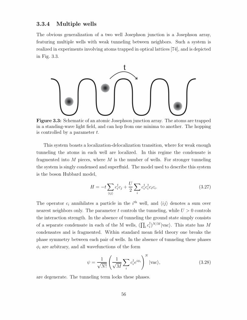
3.3.4 Multiple wells
The obvious generalization of a two well Josephson junction is a Josephson array,
featuring multiple wells with weak tunneling between neighbors. Such a system is
realized in experiments involving atoms trapped in optical lattices [74], and is depicted
in Fig. 3.3.
Figure 3.3: Schematic of an atomic Josephson junction array. The atoms are trappedin a standing-wave light field, and can hop from one minima to another. The hoppingis controlled by a parameter t.
This system boasts a localization-delocalization transition, where for weak enough
tunneling the atoms in each well are localized. In this regime the condensate is
fragmented into M pieces, where M is the number of wells. For stronger tunneling
the system is singly condensed and superfluid. The model used to describe this system
is the boson Hubbard model,
H = −t∑
〈ij〉c†icj +
U
2
∑
i
c†ic†icici. (3.27)
The operator ci annihilates a particle in the ith well, and 〈ij〉 denotes a sum over
nearest neighbors only. The parameter t controls the tunneling, while U > 0 controls
the interaction strength. In the absence of tunneling the ground state simply consists
of a separate condensate in each of the M wells, (∏
i c†i)
N/M |vac〉. This state has M
condensates and is fragmented. Within standard mean field theory one breaks the
phase symmetry between each pair of wells. In the absence of tunneling these phases
φi are arbitrary, and all wavefunctions of the form
ψ =1√N !
(
1√M
∑
i
c†ieiφi
)N
|vac〉, (3.28)
are degenerate. The tunneling term locks these phases.
56

An ingenious method of finding the phase boundary between localized and delo-
calized regimes was introduced by Fisher et al. [75] and recently revisited by Oosten
et al. [76]. This phase boundary also separates the fragmented and singly condensed
regimes. Fisher’s approach is based upon the observation is that in the localized
regime the interactions dominate over tunneling, and one cannot used approxima-
tions where the interactions are treated as small. In this approach, one instead
approximates the hopping term c†icj , expanding the field operators in this term as
ci = ψ + δci, where ψ = 〈ci〉 is the superfluid order parameter, which I take to be
real. In the localized state ψ = 0, while in the superfluid state |ψ|2 approximates the
density of particles. To first order in the fluctuation the kinetic term is
c†icj ≈ ψ2 + ψ(deltacj + δc†i ) = ψ(cj + c†i) − ψ2. (3.29)
Introducing a chemical potential µ the effective mean-field Hamiltonian reads
H =∑
i
[
−2tdψ(ci + c†i ) − µc†ici + (U/2)c†ic†icici
]
(3.30)
+2dtψ2M
where d is the number of nearest neighbors, and M is the number of sites. Note that
the different sites are decoupled. Self-consistency requires that ψ = 〈ci〉.This approximate Hamiltonian can be analyzed much like the asymmetric Joseph-
son junction in Section 3.7.1. Each site i decouples, and the wavefunction of the i′th
site is |f〉 =∑
j fj(c†i)
j |vac〉/√j!. The coefficients fi obey a difference equation with
constraints,
(E + µj − Uj(j − 1)/2)fj + 2tdψ√
j + 1fj+1 (3.31a)
+ 2tdψ√
jfj−1 = 0∑
j
|fj |2 = 1 (3.31b)
∑
j
j|fj |2 = N/M (3.31c)
∑
j
(f ∗j fj+1
√
j + 1) = ψ. (3.31d)
Within this approximation the single particle density matrix is
〈c†icj〉 = δij(N/M) + (1 − δij)|ψ|2, (3.32)
which has one eigenvalue of size N/M + (M − 1)|ψ|2, and M − 1 eigenvalues of size
N/M − |ψ|2. As expected, the state is singly condensed when |ψ|2 ∼ N/M .
57
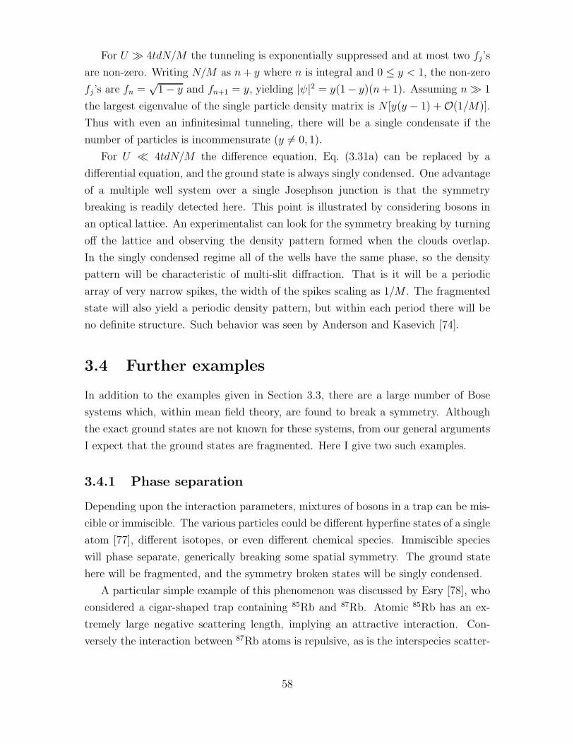
For U ≫ 4tdN/M the tunneling is exponentially suppressed and at most two fj’s
are non-zero. Writing N/M as n+ y where n is integral and 0 ≤ y < 1, the non-zero
fj ’s are fn =√
1 − y and fn+1 = y, yielding |ψ|2 = y(1− y)(n+ 1). Assuming n≫ 1
the largest eigenvalue of the single particle density matrix is N [y(y − 1) + O(1/M)].
Thus with even an infinitesimal tunneling, there will be a single condensate if the
number of particles is incommensurate (y 6= 0, 1).
For U ≪ 4tdN/M the difference equation, Eq. (3.31a) can be replaced by a
differential equation, and the ground state is always singly condensed. One advantage
of a multiple well system over a single Josephson junction is that the symmetry
breaking is readily detected here. This point is illustrated by considering bosons in
an optical lattice. An experimentalist can look for the symmetry breaking by turning
off the lattice and observing the density pattern formed when the clouds overlap.
In the singly condensed regime all of the wells have the same phase, so the density
pattern will be characteristic of multi-slit diffraction. That is it will be a periodic
array of very narrow spikes, the width of the spikes scaling as 1/M . The fragmented
state will also yield a periodic density pattern, but within each period there will be
no definite structure. Such behavior was seen by Anderson and Kasevich [74].
3.4 Further examples
In addition to the examples given in Section 3.3, there are a large number of Bose
systems which, within mean field theory, are found to break a symmetry. Although
the exact ground states are not known for these systems, from our general arguments
I expect that the ground states are fragmented. Here I give two such examples.
3.4.1 Phase separation
Depending upon the interaction parameters, mixtures of bosons in a trap can be mis-
cible or immiscible. The various particles could be different hyperfine states of a single
atom [77], different isotopes, or even different chemical species. Immiscible species
will phase separate, generically breaking some spatial symmetry. The ground state
here will be fragmented, and the symmetry broken states will be singly condensed.
A particular simple example of this phenomenon was discussed by Esry [78], who
considered a cigar-shaped trap containing 85Rb and 87Rb. Atomic 85Rb has an ex-
tremely large negative scattering length, implying an attractive interaction. Con-
versely the interaction between 87Rb atoms is repulsive, as is the interspecies scatter-
58

ing. Thus it is energetically favorable for the two atoms to phase separate, maximizing
the scattering between 85Rb atoms, and minimizing the interspecies scattering.
By solving the Gross-Pitaevskii equation, Esry was able to show that for suffi-
ciently large number of 87Rb atoms, the mean field ground state broke parity sym-
metry, with all of the 87Rb atoms at one end of the cigar and all of the 85Rb atoms
at the other. The true ground state involves a linear superposition of both symmetry
breaking states. More detailed discussion of this phenomena can be found in [79] and
references within.
3.4.2 Vortex structures
As observed experimentally, a rotating Bose condensate may contain vortices [10, 80].
Except in the case of a single straight vortex line, rotational invariance is broken by
the presence of these vortices, and the true ground state will be fragmented. The
fragmentation of finite temperature vortex arrays is discussed in Section 3.5
3.5 Finite temperature
Fragmentation is more prevalent at finite temperature than at zero temperature. The
basic reason is that when the temperature is larger than the tunneling energy, the
phases between different condensates are randomized by thermal fluctuations. This
notion is easily demonstrated by a non-interacting Josephson junction, governed by
the Hamiltonian
H = −t(a†b+ b†a). (3.33)
This Hamiltonian is diagonal in the basis of symmetric and asymmetric states, for
which the creation operators are (a† + b†)/√
2, and (a†− b†)/√
2, so the single particle
density matrix will be diagonal in this basis. At zero temperature only the symmet-
ric state is occupied, and there is a single condensate. At very large temperature
each of these states will be equally occupied so the system will be fragmented. For
intermediate temperatures, the occupation of each of these states is
nsa
=
∑N/2m=−N/2(N/2 ±m)e2tβm
∑N/2m=−N/2 e
2tβm(3.34)
=N
2∓(
N + 1
2coth(βt(N + 1)) − 1
2coth(βt)
)
. (3.35)
The upper and lower signs are used for the symmetric and antisymmetric states.
There is a smooth crossover between a singly condensed state at T = 0, and a
59

1 2 3 4 5 6 7 8 9 10kB TN t
N2
NΛ
Figure 3.4: Eigenvalues of non-interacting Josephson junction at finite temperature.The temperature is scaled by the tunneling t. At zero temperature there is one largeeigenvalue, while at high temperature both eigenvalues are of the same size.
fragmented state at T ≫ Nt/kB. These eigenvalues are plotted in Fig. 3.4.
A qualitatively different example of how finite temperature effects fragment a
condensate is a vortex lattice. Imagine a bucket of 4He rotating at frequency Ω. The
ground state of the system will contain a triangular array of vortices with nv vortices
per unit area. At finite temperature the vortex lattice will be thermally excited,
giving rise to a decay in the phase correlations across the sample. Let ψ(r) be the
superfluid order parameter coarse grained on a scale large compared to the vortex
spacing. According to [81], for large separations |r − r′|, the correlation function
〈ψ∗(r′)ψ(r′)〉 decays as |r−r′|−η, where η = 1/(3π2ρrvΛ2) is proportional to the ratio
of the distance between particles to the distance between vortices. This expression is
correct as |r − r′| becomes large. Here the particle number density is ρ, the thermal
wavelength is Λ =√
2π/mkbT and the distance between vortices is rv. This algebraic
decay of correlations in real space corresponds to an algebraic decay in momentum
space. For η < 3, the occupation of the k = 0 mode scale as N0 ∼ L3−η, and as as
k → 0 the k 6= 0 modes scale as Nk ∼ kη−3. Thus the number of macroscopically
occupied modes scale as Lη.
For a typical helium experiment, η < 10−8, and the depletion caused by this effect
is negligible. Experiments on alkali gases at MIT [82] create a vortex lattice with
rv ∼ 5µm and a particle density ρ ∼ 1014cm−3, giving a rough estimate of η ∼ 10−3,
which is also a minor correction. Experiments with smaller vortex lattices in Paris
60

[10] have a similar vortex spacing rv ∼ 2µm, and density ρ ∼ 1014cm−3, yielding
a comparable value for η. Although vortex lattices in current experiments are not
thermally fragmented, there does not appear to be any fundamental impediment to
making η larger.
3.6 Summarizing remarks
Bose condensation is a very robust phenomenon. The fragmentation of a singly con-
densate into many condensates is therefore a surprising and unexpected phenomenon.
In all cases that I have explored, the root cause of fragmentation is the presence of
a symmetry which can be broken by an infinitesimal perturbation. Consequently,
fragmentation is ubiquitous, but also very fragile and difficult to detect.
3.7 Mathematical details
3.7.1 Josephson junctions
In this Section I present an analysis of both symmetric and asymmetric Josephson
junctions. Many of these results can be found elsewhere (for example, [16, 83, 84]),
but it is useful to revisit them in a manner which is tied into the present discussion.
Symmetric junctions
Here I analyze the crossover of a symmetric Josephson Junction from a singly con-
densed to a fragmented ground state. The Hamiltonian of an ideal junction is
H = −t(a†b+ b†a) − ga†b†ba, (3.36)
where a and b are annihilation operators for two spatially separated wells, t is a
tunneling matrix element, and g parameterizes the interactions. I focus on repulsive
interactions, g > 0.
As discussed by Leggett [16], the system described by Eq. (3.36), has three distinct
behaviors. For t≪ g/N , the Fock regime, no tunneling occurs. For g/N ≪ t≪ Ng,
the Josephson regime, tunneling occurs at a rate governed by the Josephson plasma
frequency ω2J = 2tgN . For Ng ≪ t, the Rabi regime, the system behaves as a
collection of non-interacting particles undergoing Rabi oscillations between the two
wells.
61

I now derive this structure and investigate the single particle density matrix using
two methods. First I explicitly calculate the ground state wavefunction in the form,
|f〉 =∑
m
fm|N/2 +m,N/2 −m〉, (3.37)
where the state |na, nb〉 contains na particles in well a and nb particles in well b. The
eigenvalue equation H|f〉 = E|f〉 is a matrix equation
[g(N2/4 −m2) + E]fm + t[(N/2 −m)(N/2 +m+ 1)]1/2fm+1 (3.38)
+ t[(N/2 +m)(N/2 −m+ 1)]1/2fm−1 = 0.
In both the Fock and Josephson regimes, fm is sharply peaked at m = 0 with width
δm≪ N1/2, and this equation may be approximated as
[g(N2/4 −m2) + E]fm + [tN/2]fm+1 + [tN/2]fm−1 = 0. (3.39)
This assumption about the width of fm is readily verified a posteriori. In the Fock
regime, t ≪ g/N , perturbation theory converges, and the ground state has fm =
δm0 +O(tN/g). The single particle density matrix is fragmented with two eigenvalues
of size (N/2)(1 +O(tN/g)). In the Josephson limit, a semiclassical approximation is
valid and the discrete eigenvalue equation can be replaced by a differential equation
(E + gN2/4)f(m) = −(tN/2)∂2mf(m) + gm2f(m), whose ground state is f(m) ∝
exp(−m2/2ξ2), with ξ4 = tN/2g. In the Josephson limit the off-diagonal matrix
element is given by 〈a†b〉 = (N/2) exp(−1/4ξ2), implying that up to exponentially
small corrections, the single particle density matrix has a single large eigenvalue
of size N , and the state is singly condensed. Note that the number fluctuations
〈(na − nb)2〉 − 〈(na − nb)〉2 are sub-Poissonian, and this regime corresponds to a
squeezed state in number-phase space. Finally, in the Rabi regime, perturbation
theory about the state (a† + b†)N |vac〉/N !2N/2 converges, and once again the state is
singly condensed.
This same structure can be understood from within Bogoliubov theory, where the
field operators a and b are expressed as a mean field plus fluctuations, a =√
N/2+ a,
b =√
N/2 + b. Adding a chemical potential µ to the Hamiltonian, and expanding to
second order in the fluctuations,
H =(
g(N/2)2 − (µ+ t)N)
+√
N/2(N/2 − (µ+ t))(a+ a† + b+ b†) (3.40)
+(gN − µ)(a†a + b†b) + (gN/4)(aa + a†a† + bb+ b†b†) − t(ab† + b†a).
Setting µ = N/2 − t eliminates the linear terms, and the quadratic terms are diago-
nalized via a Bogoliubov transformation. The resulting depletion is Nd = (ǫ−E)/2E,
62

where ǫ = 2t+ gN/2, and E2 = ǫ2 − (gN/2)2. For t≫ Ng the depletion is negligible,
Nd ≪ 1. This vanishing depletion characterizes the Rabi regime. For Ng ≫ t≫ g/N
the depletion is Nd =√
gN/32t+O((t/gN)0), which is much greater than 1 but much
less than N , as one expects in the Josephson regime. For g/N ≫ t the depletion is of
order 1, signalling a breakdown of the Bogoliubov theory, and the system enters the
Fock regime.
Asymmetric junctions
In Section 3.7.1 I briefly describe how fragmentation appears in a double well system.
A crucial point in that example is that the two levels are degenerate. Here I extend
the model to that of an asymmetric double well, finding that as long as the energy
difference between the two states is less than the interaction energy gN , then the
asymmetry plays a minor role, and the system possesses the same three regimes:
Rabi, Josephson, and Fock. When the energy difference between the two states is
greater than gN , the system is always singly condensed. The Fock regime of the
asymmetric well shows additional structures as one changes the bias.
The asymmetric double-well system is described by a Hamiltonian
H = −t(a†b+ b†a) + ǫ(a†a− b†b)
+(g/2)(a†a†aa+ b†b†bb). (3.41)
The wells are split by an energy 2ǫ and there is a tunneling of strength t between
them. I will assume repulsive interactions g > 0, and with no loss of generality take
ǫ ≥ 0.
For small asymmetries, ǫ≪ g/N , the analysis performed for the symmetric system
works without modification, and one has three regimes: Rabi, Josephson, and Fock,
their boundaries unaffected by ǫ. Larger asymmetries are more complicated; one
has the same three regimes, but their boundaries are shifted, and the Fock regime
contains extra structure. I will first address this extra structure, and then consider
the boundaries of these regimes.
Writing the wavefunction as Eq. (3.37), the f ’s obey the discrete eigenvalue equa-
tion
[g(N/2 −N2/4 −m2) − 2ǫm+ E]fm + t[(N/2 −m)(N/2 +m+ 1)]1/2fm+1
+ t[(N/2 +m)(N/2 −m+ 1)]1/2fm−1 = 0.
(3.42)
63

The extreme limit of the Fock regime is when t = 0. In this limit, the eigen-
states are of the form fm = δmm, for any integer m, corresponding to the state
(a†)N/2+m(b†)N/2−n|vac〉. When ǫ < gN/2, the ground state has m equal to the clos-
est integer to −ǫ/g. This state is degenerate when −ǫ/g is half integral.
Adding a sufficiently small t will only change this structure near the degeneracy
points. To find the implications of t 6= 0, I take ǫ = (n+ 1/2 + δ)g, where n < N/2 is
an integer, and δ is a small number with |δ| < 0.5. In this case the only non-zero f ’s
will be f−n and f−n−1, and in this restricted space the eigenvalue equation becomes
(
E − gδ ∆
∆ E + gδ
)(
f−n
f−n−1
)
= 0, (3.43a)
∆ = t√
(N/2 − n)(N/2 + n+ 1), (3.43b)
where E = E + gn + gn2 + gN/2 − gN2/4 + gδ + 2gnδ. The ground state energy
is given by E2 = (gδ)2 + t2(N/2 − n)(N/2 + n + 1). This state has the form ψ =
α|N/2+n,N/2−n〉+β|N/2+n+1, N/2−n−1〉, with single-particle density matrix
elements
〈a†a〉 = N/2 + n+ |β|2 (3.44a)
〈a†b〉 = βα√
(N/2 − n)(N/2 + n + 1) (3.44b)
〈b†a〉 = βα√
(N/2 − n)(N/2 + n + 1) (3.44c)
〈b†b〉 = N/2 − n− |β|2. (3.44d)
The system has its greatest level of coherence when δ = 0, where the coefficients α
and β are equal and the two eigenvalues are
EV = N/2 ± (1/4)√N2 + 2N + 12n2 + 12n+ 4. (3.45)
For large N and small n this leads to an eigenvalue of size 3N/4 and another of N/4.
It is startling that the tunneling of a single particle leads to such a large increase in
the coherence of the single particle density matrix.
The system has its lowest level of coherence when δ = −1/2, where the coefficient
β vanishes, and the two eigenvalues are
EV = N/2 ± n. (3.46)
The structure discussed here is clearly seen in Fig. 3.5 where I plot the size of the
largest eigenvalue of the single particle density matrix as a function of t and ǫ. In
this plot, N = 10 particles are used, and the energy scale is set by taking g = 1.
64
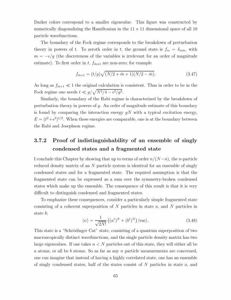
Darker colors correspond to a smaller eigenvalue. This figure was constructed by
numerically diagonalizing the Hamiltonian in the 11× 11 dimensional space of all 10
particle wavefunctions.
The boundary of the Fock regime corresponds to the breakdown of perturbation
theory in powers of t. To zeroth order in t, the ground state is fm = δmm, with
m = −ǫ/g (the discreteness of the variables is irrelevant for an order of magnitude
estimate). To first order in t, fm±1 are non-zero; for example
fm+1 = (t/g)√
(N/2 + m+ 1)(N/2 − m). (3.47)
As long as fm+1 ≪ 1 the original calculation is consistent. Thus in order to be in the
Fock regime one needs t≪ g/√
N2/4 − ǫ2/g2.
Similarly, the boundary of the Rabi regime is characterized by the breakdown of
perturbation theory in powers of g. An order of magnitude estimate of this boundary
is found by comparing the interaction energy gN with a typical excitation energy,
E = (t2+ǫ2)1/2. When these energies are comparable, one is at the boundary between
the Rabi and Josephson regime.
3.7.2 Proof of indistinguishability of an ensemble of singly
condensed states and a fragmented state
I conclude this Chapter by showing that up to terms of order n/(N−n), the n-particle
reduced density matrix of an N particle system is identical for an ensemble of singly
condensed states and for a fragmented state. The required assumption is that the
fragmented state can be expressed as a sum over the symmetry-broken condensed
states which make up the ensemble. The consequence of this result is that it is very
difficult to distinguish condensed and fragmented states.
To emphasize these consequences, consider a particularly simple fragmented state
consisting of a coherent superposition of N particles in state a, and N particles in
state b;
|ψ〉 =1√2N !
(
(a†)N + (b†)N)
|vac〉. (3.48)
This state is a “Schrodinger Cat” state, consisting of a quantum superposition of two
macroscopically distinct wavefunctions, and the single particle density matrix has two
large eigenvalues. If one takes n < N particles out of this state, they will either all be
a atoms, or all be b atoms. So as far as any n particle measurements are concerned,
one can imagine that instead of having a highly correlated state, one has an ensemble
of singly condensed states, half of the states consist of N particles in state a, and
65

0.01 0.1 1 10. 100.Ε
0.001
0.01
0.1
1
10.
100.
t
Figure 3.5: Density plot of the largest eigenvalue λmax of the single particle densitymatrix of a system of N = 10 particles in an asymmetric double well where theinteractions are characterized by g = 1, the tunneling by t and the asymmetry byǫ [see Eq. (3.41)]. Black corresponds to the minimum value λmax = 5, while whitecorresponds to the maximum value λmax = 10. There are three distinct regimes,the Fock regime (darker area) where t is perturbative, the Rabi regime where g isperturbative, and an intermediate Josephson regime. The boundary between theJosephson and Rabi regime lies within the white area of the plot. The plateaus inthe Fock regime are understood by setting t = 0, in which case there are a fixedintegral number of particles in each well. As one tilts the wells it becomes favorableto increase the number of particles in the lower well. At the boundaries between theplateaus there is a marked increase in the size of the largest eigenvalue coincidentwith an avoided crossing of energy levels.
66

the other half of N particles in state b. One must perform a huge conceptual leap to
replace Eq. (3.48) with a classical ensemble of condensed states. Such a replacement
means that as far as any individual run of our experiment is concerned, the state is
condensed into either (a†)N |vac〉 or (b†)N |vac〉.In a more generic situation one begins with a fragmented state of the form
|f〉 ∝∑
g∈G
|g〉. (3.49)
The states |g〉 are singly condensed, and are labeled by elements of the symmetry
group G. For example, Eq. (3.6) is a fragmented state of this form. The normalization
of |f〉 is not important. The (many particle) density matrix corresponding to this
state is
ρf = |f〉〈f | ∝∑
g,g′
|g〉〈g′|. (3.50)
The n-particle reduced density matrices ρ(n)f are formed when all but n of the particles
are traced over. All n particle properties of the system are encoded in ρ(n). These
reduced density matrices are most familiar in a position basis, where they are given
by
ρ(n)f (r1, . . . rn, r
′1 . . . r
′n) (3.51)
∝∑
g,g′
〈g|ψ†(rn) · · ·ψ†(r1)ψ(r1) · · ·ψ(rn)|g′〉.
In this equation, ψ(r) is the field operator, which annihilates a particle at position r.
I have neglected the normalization of this density matrix, as it can be simply restored
by equating the trace of ρ(n) to n!.
I now compare this fragmented state to an ensemble of condensed states, with a
density matrix
ρi ∝∑
g∈G
|g〉〈g|. (3.52)
The index i is chosen to indicate that this is an incoherent (classical) sum of condensed
states. Analogous to Eq. (3.51), the reduced density matrices are
ρ(n)i (r1, . . . rn, r
′1 . . . r
′n) ∝ (3.53)
∑
g
〈g|ψ†(rn) · · ·ψ†(r1)ψ(r1) · · ·ψ(rn)|g〉.
Depletion plays no role in my argument, so for simplicity I take
|g〉 = (N !)−1/2
(∫
d3r ψ†(r)φg(r)
)N
|vac〉 (3.54a)
= (N !)−1/2(ψ†g)
N |vac〉, (3.54b)
67

where φg(r) is the wavefunction for the single particle state which is macroscopically
occupied, and ψ†g is the operator which creates a particle in this state. Using this
ansatz,
ρ(n)f ∝
∑
g,g′
〈vac|(ψg)Nψ†(rn) · · ·ψ†(r1)
×ψ(r1) · · ·ψ(rn)(ψ†g′)
N |vac〉(3.55a)
∝∑
g,g′
(
φ∗g(rn) · · ·φ∗
g(r1)
× φg′(r1) · · ·φg′(rn)) [Dgg′ ]N−n .
(3.55b)
Generically the overlap Dgg′ = [∫
d3rφ∗g(r)φg′(r)] is peaked about g = g′, and for
N ≫ n, the factor (Dgg′)N−n can be replaced by a Gaussian of width O(1/
√N − n).
Consequently, I can expand the rest of the sum, [φ∗g(rn) · · ·φ∗
g(r1)φg′(r1) · · ·φg′(rn)],
to quadratic order about g = g′. This quadratic term is at most of order n, yielding
ρ(n)f ∝
∑
g
(φ∗g(rn) · · ·φ∗
g(r1)φg′(r1) · · ·φg′(rn) (3.56)
+O (n/(N − n)) ,
which to leading order equals ρ(n)i .
68

Chapter 4
Persistent Currents
The ability to support metastable current carrying states in multiply connected
settings is one of the prime signatures of superfluidity. In this Chapter I calculate
the stability of these currents against decay via thermal fluctuations, finding that the
lifetimes of metastable currents can be tuned from much longer to much shorter than
experimental time scales. The research presented in this Chapter was performed in
collaboration with Paul Goldbart and Yuli Lyanda-Geller, and is published in Physical
Review A [85].
4.1 Introduction
Multiply connected superfluid and superconducting systems can support states in
which a persistent macroscopic particle current flows. While not truly eternal, these
states can have extraordinarily long life times, their decay requiring the occurrence
of certain relatively infrequent but nevertheless topologically accessible (quantum or
thermal) collective fluctuations [86, 87, 88, 89]. The purpose of this Chapter is to
address, theoretically, the ability of BEC alkali gas systems in multiply connected
settings to support metastable current carrying states, and to address the stability
and decay of such states via thermal fluctuations.
From a theoretical perspective, superfluidity is naturally addressed in a multiply
connected setting, particularly that of a thin torus where the fluid can be treated in
a quasi one dimensional manner. Thus there are a fairly large number of theoretical
works looking at Bose gases in a toroidal trap [72, 73, 90, 91]. Several proposals
for experimental multiply connected structures have been suggested. Figure 4.1 il-
lustrates the toroidal geometry which I study here. A similar geometry has been
realized at JILA, in a disk magnetic trapped filled with two hyperfine states of ru-
69

r
Rz
φr
Figure 4.1: Envisaged geometry of a trap supporting metastable current carryingBEC states. The condensate healing length ξMF is regarded as being small, comparedwith the circumference of the torus L (= 2πr), but larger than its thickness R.
bidium [92]. One of the species migrates to the center of the trap, leaving a toroidal
volume for the other species, as depicted in Fig. 4.2. Another mechanism for creating
a toroidal trap is to take a conventional simply connected trap, and shine a narrow
laser beam through its center. When blue detuned from an atomic transition, such
a laser beam presents a repulsive dipole force which restricts the atoms to a toroidal
region. Microfabricated toroidal traps [94] and all optical toroidal traps [93] have also
been suggested.
4.2 Gross Pitaevskii functional
I adopt a phenomenological description in which the state of the BEC system is
characterized by a macroscopic wavefunction Ψ(r, t), in terms of which the condensate
density n and current density j are given by
n(r) = |Ψ(r)|2 , (4.1a)
j(r) =~
2im(Ψ∗∇Ψ − Ψ∇Ψ∗) . (4.1b)
70

a
b
Figure 4.2: A multiply connected trap realized at JILA [92]. In a) a standarddisk shaped harmonic trap is shown. In b) one sees the trap filled with two atomichyperfine states. Due to their relative buoyancies, one state migrates to the centerleaving a toroidal volume for the second species.
71

The energy F of the state is given by the Gross Pitaevskii form
F =
∫
d3r
~2
2m|∇Ψ|2 + (V (r) − µ) |Ψ|2 +
g
2|Ψ|4
, (4.2)
where m is the mass of an individual atom, V (r) is an effective external potential
describing the magnetic and optical confinement of the atoms, µ is the chemical po-
tential, and g (≡ 4π~2a/m) represents the interatomic interaction, with a being an
effective scattering length. Equation (4.2) can be derived from the microscopic equa-
tions of motion by making the variational ansatz that all of the condensed particles
are in a state with wavefunction Ψ(r, t) (see Appendix C.4.1). This equation ignores
the presence of noncondensed particles, which play the important role of a bath of
energy and angular momentum that will enable the persistent currents to decay. The
techniques of Chapter 6 provide kinetic equations to describe these noncondensed
particles, but the problem at hand is dominated by energetics and not kinetics, so
these detailed equations are not needed.
I consider trap potentials V (r) that confine the gas to a cylindrically symmetric
toroidal region (Fig. 4.1). Hence, V depends only on r and z, where r, φ, z are
the usual cylindrical polar coordinates. Moreover, I restrict my attention to systems
in which the circumference of the torus L (= 2πr) is considerably greater than the
condensate healing length ξMF [≈ (~2/mgn)1/2, where n is related to the maximum
particle-density], and the thickness of the torus R is comparable to or smaller than
ξMF. This corresponds to a regime of low condensate-density. There are two main
reasons for considering this setting: (i) there would be no locally-stable current-
carrying states if L were comparable to or smaller than ξMF; (ii) for thicker samples
(i.e. R > ξMF), the relevant dissipative processes by which the persistent current
decays become significantly more complicated (ultimately involving the nucleation of
vortex rings) [95].
4.3 Thermally activated processes
This Chapter is concerned with events in which the system decays from some metastable
current-carrying state Ψm (which is a local minimum of F) to a lower-energy (and
typically more stable) state via a thermal fluctuation.1 The current decays through a
dissipative process during which the condensate density shrinks in magnitude over a
1 In the temperature regime considered here (i.e. T ∼ Tc), quantum fluctuations contribute less
significantly than thermal fluctuations, and will therefore be disregarded.
72

region whose length is comparable to ξMF. Dynamically, one can envisage this process
as occurring via the passage of a vortex across the sample (Fig. 4.3): a free-energy
barrier must be overcome for this event to occur. The height of this barrier δF is given
by the difference between the free energy of (the metastable state) Ψm and that of the
transition state Ψt, i.e. the lowest possible free-energy high point en-route through
configuration space between the initial and final metastable states. A schematic draw-
ing of the free energy landscape is shown in Fig. 4.4. This thermally activated process
should occur at a rate ω0e−δF/kT , where, as shall be discussed later, the attempt fre-
quency ω0 does not contribute significantly to the temperature-dependence of the
rate.
4.3.1 Metastable states
In order to calculate the barrier heights, I first identify the collection of metastable
current carrying states Ψm and the intervening saddle point states Ψt. Both
families of states are stationary points of F , and therefore satisfy the time independent
Gross Pitaevskii equation
δFδΨ∗ = − ~
2
2m∇2Ψ + (V (r) − µ)Ψ + g|Ψ|2Ψ = 0, (4.3)
subject to periodic boundary conditions in the coordinate φ.
Near Tc, where the thermal fluctuations are most important, the number of con-
densed particles is small, and it is reasonable to assume that the interaction energy
is small compared to the transverse level spacing. This is the quasi 1D limit where
the wavefunction may be written as
Ψ(r, φ, z) = F (φ)R(r, z). (4.4)
The transverse wavefunction R is the lowest energy solution of the eigenproblem,
− ~2
2m
(
r−1∂rr ∂r + ∂2z
)
R + V (r, z)Rν = λR. (4.5)
Inserting the ansatz (4.4) into (4.3) gives a one dimensional Gross Pitaevskii equation
for the wavefunction F (φ),
F ′′ + αF − βΓ|F |2F = 0, (4.6)
where primes denote derivatives with respect to φ, and the coefficients are
α ≡ 2mr2 (µ− λ) /~2, (4.7a)
β ≡ 2mr2g/~2, (4.7b)
Γ ≡∫
dz
∫
r dr |R|4. (4.7c)
73

a)
b)
Figure 4.3: The phase slip event can be thought of as occurring when a “virtual”vortex crosses through the toroidal condensate. In a) one sees a toroidal cloud withtwo units of circulation per particle. This circulation can be thought of as due to thepresence of two vortices in the center of the ring. In b) one of the vortices attemptsto cross the condensate. This phase slip event reduces the angular momentum of eachparticle by ~. There is a barrier to this process because the density has to vanish atthe point where the vortex crosses, requiring a larger density elsewhere. This densitybuildup costs energy.
74

Figure 4.4: Schematic drawing of free energy landscape. The vertical axis shows theenergy of a state. The horizontal axis is a relevant reaction coordinate (for example,the mean angular momentum per particle). Phase slip events take the system from oneminima to another. The extrema are labeled by pictures which depict the positions ofthe “virtual vortices.” The number of such vortices gives the circulation each particlein the toroidal trap carries. In the transition states, a vortex is escaping.
75

Corrections to this simple approximation are discussed in [85].
The uniform current carrying states are described by (4.4) with F (φ) = fmeiSM ,
with fm constant, and SM winding uniformly,
f 2m = Nm/2π = (α− n2
m)/βΓ, (4.8a)
Sm = nmφ, (4.8b)
with integral nm. In these expressions, Nm is the number of condensed particles.
Physically, Γ−1 is R2L, the volume occupied by the condensate. By considering the
second variation of F it can be readily shown that these states are local minima (and
hence metastable) provided nζm ≤ 1, where ζm ≡ (4π/βΓNm)1/2 ≈ 2πξMF/L is the
dimensionless coherence length. (This limit on the maximum stable value of nm is
the same as one would find using Landau’s criterion for the critical velocity.)
4.3.2 Transition states
As is readily verified [85], the transition states Ψt = ft eiStR are given by
f 2t = (Nt/2π)
(
1 − ∆2sech2(∆φ/ζt))
, (4.9a)
f 2t ∂φSt = (Nt/2π)nt. (4.9b)
Far from a region of length ξMF, the amplitude ft is constant (f 2t ∼ Nt/2π) and the
phase St winds uniformly (St ∼ ntφ). The coefficients in Eq. (4.9) appear simplest
when expressed in terms of the dimensionless coherence length ζt ≡ (4π/βΓNt)1/2:
Nt/2π = (α− n2t )/βΓ, (4.10a)
nt = n− π−1 cos−1(nt ζt), (4.10b)
∆2 = 1 − (nt ζt)2. (4.10c)
As Nm and Nt differ only by quantities of order ξMF/L, either of them may be used to
characterize the number of condensed particles. A typical transition state is depicted
in Fig. 4.5. The transition states must have the property that they are saddle points
of F with only one direction of negative curvature. (This unstable direction is the
relevant reaction coordinate.) Within the quasi 1D approximation this condition is
always true. In [85] I consider corrections to this approximation and show that this
condition remains true as long as ξMF > R.
Having found the relevant states, I now calculate the free energy barrier for dis-
sipative fluctuations. Straightforward substitution shows that states, Ψ = f eiSR,
76
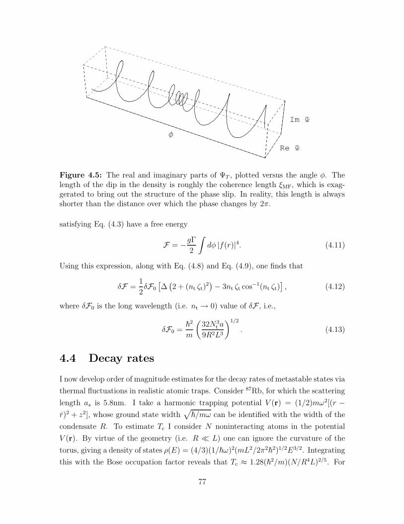
Re Y
Im Y
Φ
Figure 4.5: The real and imaginary parts of ΨT , plotted versus the angle φ. Thelength of the dip in the density is roughly the coherence length ξMF, which is exag-gerated to bring out the structure of the phase slip. In reality, this length is alwaysshorter than the distance over which the phase changes by 2π.
satisfying Eq. (4.3) have a free energy
F = −gΓ2
∫
dφ |f(r)|4. (4.11)
Using this expression, along with Eq. (4.8) and Eq. (4.9), one finds that
δF =1
2δF0
[
∆(
2 + (nt ζt)2)
− 3nt ζt cos−1(nt ζt)]
, (4.12)
where δF0 is the long wavelength (i.e. nt → 0) value of δF , i.e.,
δF0 =~
2
m
(
32N3t a
9R2L3
)1/2
. (4.13)
4.4 Decay rates
I now develop order of magnitude estimates for the decay rates of metastable states via
thermal fluctuations in realistic atomic traps. Consider 87Rb, for which the scattering
length as is 5.8nm. I take a harmonic trapping potential V (r) = (1/2)mω2[(r −r)2 + z2], whose ground state width
√
~/mω can be identified with the width of the
condensate R. To estimate Tc I consider N noninteracting atoms in the potential
V (r). By virtue of the geometry (i.e. R ≪ L) one can ignore the curvature of the
torus, giving a density of states ρ(E) = (4/3)(1/~ω)2(mL2/2π2~
2)1/2E3/2. Integrating
this with the Bose occupation factor reveals that Tc ≈ 1.28(~2/m)(N/R4L)2/5. For
77

example, if one assumes that N ≈ 106, Nt ≈ 2.5 × 10⁴, R ≈ 1µm, and L ≈ 100µm
then δF0 /kB = 3.2µK, and Tc = 0.28µK. The barrier height is sensitive to changes
in Nt, and can therefore be manipulated by heating or cooling the sample.
The Arrhenius formula for the decay rate in terms of the barrier height is Γ ≈ω0e
−δF/kT . The attempt frequency ω0 can be estimated by using the value of the
microscopic relaxation time τ , together with the assumption that each coherence
volume in the sample fluctuates independently [86]. A realistic estimate for τ is the
classical collision time for a dilute gas [i.e. τ−1 ∼ σnv ∼ a2(N/V )(kBT/m)1/2 ∼5 × 10⁴ Hz], giving lifetimes for the metastable states on the order of seconds. Even
beyond the limits of validity of this calculation, one expects δF to be a monotonically
increasing function of the density. Hence, the barriers can be extremely large at low
temperatures, allowing a continuous tuning of the metastable state lifetime from
microseconds to times longer than the lifetime of the condensate.
4.5 Detection and creation
I now discuss two of the issues necessary for the experimental testing of the predictions
presented in this Chapter. First, how does one create a current carrying state? The
most promising techniques for creating persistent currents are those that have been
used to create vortices [10, 80, 82]. The simplest approach is to stir the condensate
by deforming and rotating the trap that contains the atoms. The other method is to
use a phase imprinting technique. Since the superfluid velocity is proportional to the
gradient of the phase, by changing the phase one can give angular momentum to the
condensate. The phase is shifted by illuminating the condensate with off resonant light
through an appropriate mask. Detailed numerical simulations of creating persistent
currents with this technique are found in [96].
The second important experimental matter is how to detect a current carrying
state. Perhaps the least difficult scheme would make use of present phonon imag-
ing techniques [97]. The experimental configuration could be as follows: A pulse of
laser light generates a local rarefaction of the condensate, which then travels as two
waves, one moving clockwise, the other counterclockwise. By nondestructive imaging
techniques one might then observe where the two waves meet, which gives the veloc-
ity of the metastable supercurrent. This is only feasible if the speed of sound c is
comparable to the velocity v with which the condensate moves around the annulus.
Linearizing Eq. (4.6) gives c = (gΓNm/2πm)1/2 ≈ 1.2mm/s, which is only 30 times
greater than v = ~/mr ≈ 46µm/s.
78

As an alternative scheme, one can perform an interference experiment where a
nonrotating condensate is overlapped with the toroidal cloud [92]. If the toroidal
cloud is rotating, the spatially varying phase will be visible in the resulting interference
pattern.
4.6 Coherent vs. incoherent pathways
Throughout this calculation I have assumed that a single condensate always exists.
More generally, the transition state could have a fragmented condensate (see Chapter
3) or even a more complicated structure with no condensation at all. Based upon the
intuition that I have gained from the study in Chapter 3, I expect that the energy of
the transition state would change much if one broadens the allowable class of states.
It should also be noted that any single measurement that tried to catch the phase slip
on film would undoubtedly see a single condensate at all times (see Section 3.2.2).
79

Chapter 5
Finite Temperature Collapse of a
Gas with Attractive Interactions
In this Chapter I present a study of the mechanical stability of the weakly interacting
Bose gas with attractive interactions. My major concern here is the role of finite
temperature, and I show that the non-condensed particles play a crucial role in de-
termining the region of stability, including providing a mechanism for collapse in the
non-condensed cloud. Furthermore, I demonstrate that the mechanical instability
prevents BCS-type “pairing” in the attractive Bose gas. I extend these results to
describe domain formation in spinor condensates. The research in this chapter was
performed with Gordon Baym, and has been published in Physical Review A [98].
5.1 Introduction
5.1.1 The system of interest
At high densities, attractive interactions drive a mechanical instability in atomic
clouds. At low densities these clouds are stabilized by quantum mechanical and
entropic effects. The presence of both these stabilizing mechanisms makes attractive
Bose gases unique. For comparison, interstellar hydrogen has a similar instability,
the Jeans instability, in which gravity competes with thermal pressure [8]; however
quantum mechanics plays no role in the stability of hydrogen clouds, and the collapse
is therefore much less rich.
Experimentally, stability and collapse has been observed in clouds of degenerate7Li [24] and 85Rb [25], both of which have attractive interactions. Previous theoretical
studies of the attractive Bose gas, typically numerical, have been limited to zero [99] or
very low [100] temperature. Here I give a simple analytic description of the region of
80

stability and threshold for collapse valid from zero temperature to well above the Bose
condensation transition, and thus provide a consistent global picture of the instability.
Contrary to previous predictions, at finite temperature the non-condensed particles
can play a significant role in the collapse.(A very recent variational calculation by
Tempere et al. [101] is capable of describing the collapse over a range of temperatures
comparable to the approach presented here.)
5.1.2 Results
My results are summarized in the phase diagram in Fig. 5.1 which shows three regions:
normal, Bose condensed, and collapsed. This third region is not readily accessible
experimentally; the system becomes unstable at the boundary (the solid line in the
figure). The gross features of the phase diagram can be understood qualitatively
with dimensional arguments similar to those in section 1.2.5. At low temperatures
the only stabilizing force is the zero-point motion of the atoms. This “quantum
pressure” (which should not be confused with the Fermi pressure which stabilizes
neutron stars) has a characteristic energy per particle, EQ ∼ ~2V −2/3/m, where ~
is Planck’s constant, V is the volume in which the cloud is confined, and m is the
mass of an atom. The attractive interactions which drive the collapse are associated
with an energy U = ~2asn/m, where n is the density, and as (= −1.45 nm for 7Li
and −20 nm for 85Rb) is the s-wave scattering length. Comparison of U with EQ
indicates that for low temperatures the density n at collapse should be n ∼ (V 2/3as)−1,
independent of temperature. At high temperatures, the stabilizing force is thermal
pressure, P = −T∂S/∂V , which is characterized by the thermal energy ET ∼ kBT .
Here comparison of U with ET indicates that at high temperatures the density of
collapse should be n ∼ mkBT/~2as, linear in temperature. The crossover between
the quantum and classical behaviors (n ∝ T 0 and n ∝ T ) occurs near Tc. The collapse,
as described here, is a phenomena in which the cloud as a whole participates, not just
the condensate.
In this Chapter, I calculate the last point of metastability against collapse. As
one approaches this point, the system will generally undergo an earlier dynamical
collapse, driven by thermally activated processes [102], as in a first order Van der
Waals transition, or quantum tunneling [103], both of which destabilize the cloud.
The actual dynamics of collapse are, however, beyond the scope of this Chapter. The
dynamics can be described by the tools of Chapter 6.
81

1 10 100
Temperature [ µK]
Density cm -3[ ]
1016
NormalCondensed
1015
1014
1013
1012
0.1
Collapsed
100010 100
Temperature [ nK]
Density cm -3[ ]
NormalCondensed
1014
1013
1012
Collapsed
a)
b)
Figure 5.1: Phase diagram, density n [cm−3] versus temperature T , for a cloud ofattractive bosons. a) For a cloud of 7Li with spatial extent L = 3.15µm and scatteringlength as = −1.45nm, corresponding to the experiments in Ref. [1], performed at Tnear 300 nK. b) For a cloud of 85Rb with scattering length as = −20nm and spatialextent L = 3µm, corresponding to the recent experiments in Ref. [2], performed at Tnear 15 nK. Note the logarithmic scales. The solid line separates the unstable (shaded)region from the stable region. The dashed line, representing the Bose condensationtransition has been continued into the collapsed region to illustrate that the two linesintersect. This diagram is drawn for a uniform but finite cloud, but can be appliedto harmonically trapped gases by taking n to be the central density in the trap.
82
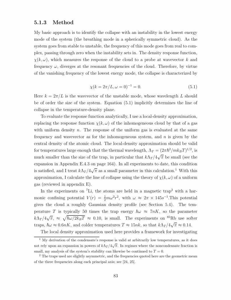
5.1.3 Method
My basic approach is to identify the collapse with an instability in the lowest energy
mode of the system (the breathing mode in a spherically symmetric cloud). As the
system goes from stable to unstable, the frequency of this mode goes from real to com-
plex, passing through zero when the instability sets in. The density response function,
χ(k, ω), which measures the response of the cloud to a probe at wavevector k and
frequency ω, diverges at the resonant frequencies of the cloud. Therefore, by virtue
of the vanishing frequency of the lowest energy mode, the collapse is characterized by
χ(k = 2π/L, ω = 0)−1 = 0. (5.1)
Here k = 2π/L is the wavevector of the unstable mode, whose wavelength L should
be of order the size of the system. Equation (5.1) implicitly determines the line of
collapse in the temperature-density plane.
To evaluate the response function analytically, I use a local-density approximation,
replacing the response function χ(k, ω) of the inhomogeneous cloud by that of a gas
with uniform density n. The response of the uniform gas is evaluated at the same
frequency and wavevector as for the inhomogeneous system, and n is given by the
central density of the atomic cloud. The local-density approximation should be valid
for temperatures large enough that the thermal wavelength, ΛT = (2π~2/mkBT )1/2, is
much smaller than the size of the trap, in particular that kΛT/4√π be small (see the
expansion in Appendix E.4.3 on page 164). In all experiments to date, this condition
is satisfied, and I treat kΛT/4√π as a small parameter in this calculation.1 With this
approximation, I calculate the line of collapse using the theory of χ(k, ω) of a uniform
gas (reviewed in appendix E).
In the experiments on 7Li, the atoms are held in a magnetic trap2 with a har-
monic confining potential V (r) = 12mω2r2, with ω ≈ 2π × 145s−1.This potential
gives the cloud a roughly Gaussian density profile (see Section 5.4). The tem-
perature T is typically 50 times the trap energy ~ω ≈ 7nK, so the parameter
kΛT/4√π, ≈
√
~ω/2kBT ≈ 0.10, is small. The experiments on 85Rb use softer
traps, ~ω ≈ 0.6nK, and colder temperatures T ≈ 15nk, so that kΛT/4√π ≈ 0.14.
The local density approximation used here provides a framework for investigating
1 My derivation of the condensate’s response is valid at arbitrarily low temperatures, as it does
not rely upon an expansion in powers of kΛT /4√
π. In regimes where the noncondensate fraction is
small, my analysis of the system’s stability can likewise be continued to T = 0.2 The traps used are slightly asymmetric, and the frequencies quoted here are the geometric mean
of the three frequencies along each principal axis; see [24, 25].
83

the interplay of condensation and collapse. Although the results are not as accurate
as can be obtained through numerical simulations (comparing with previous numeri-
cal work [100], I find that my results are always well within a factor of two of those
calculated using more sophisticated models), the conceptual and computational ad-
vantages of working with a uniform geometry far outway any loss in accuracy. Due to
their simplicity, the arguments used here provide an essential tool in choosing which
parameter ranges to investigate in future experiments and computations.
The tools introduced to discuss the collapse of an attractive gas can also be used
to describe other instabilities in trapped Bose gases. In Section 5.5 and 5.6, I apply
these methods to the problem of BCS type pairing between bosons, and towards
domain formation in spinor condensates.
5.2 Simple limits
5.2.1 Zero temperature
To illustrate my approach, I first consider the stability of a zero temperature Bose
condensate. The excitation spectrum of a uniform gas is [105]:
~2ω2
k = ε2k + 2gnεk ≡ E2
k , (5.2)
where εk = ~2k2/2m and g = 4π~
2as/m. In the attractive case, g < 0, all long
wavelength modes with εk < 2|g|n have imaginary frequencies and are unstable. A
system of finite size L only has modes with k > 2π/L, and for larger k has an
excitation spectrum similar to Eq. (5.2). If |g|n < ~2π2/mL2, the unstable modes are
inaccessible and the attractive Bose gas is stable.
This information is included in the density response function χ(k, ω) of the dilute
zero-temperature gas [104], which gives the change in density n induced by an external
potential U , of wavevector k and frequency ω, coupled to the density:
χ(k, ω) =δn
δU=
nk2
m(ω2 −E2k/~
2)(5.3)
The poles of χ are at the excitation energies, ±Ek. In particular, χ(k = 2π/L, ω = 0)
diverges when |g|n = ~2π2/mL2.
5.2.2 High temperature (T ≫ Tc)
To illustrate the procedure further I calculate the stability of an attractive Bose gas
at temperatures much larger than Tc, where thermal pressure is the predominant
84

stabilizing force. Quantum effects are negligible in this limit, and the line of collapse
is simply the spinodal line of the classical liquid-gas phase transition,3 as characterized
by Mermin [106]. One can neglect finite size effects, and look for an instability in the
uniform gas at zero wavevector, k = 0, corresponding to finding where χ(k = 0, ω = 0)
diverges. The susceptibility χ(0, 0) = −∂n/∂µ (where µ is the chemical potential),
is proportional to the compressibility of the system, which diverges when the gas
becomes unstable.
At high temperature one can work in the Hartree Fock approximation, where the
density is given by the self consistent solution of
n =
∫
d3p
(2π~)3
1
eβ(ǫp−µ) − 1, (5.4)
with Hartree Fock quasiparticle energies ǫp = εp + 2gn; here β = 1/kBT . In the
classical limit (βµ ≪ −1), n = eβ(µ−2gn)/Λ3T . The response χ(0, 0) has the structure
of the random phase approximation (RPA),
χ(k, ω) =χ0(k, ω)
1 − 2gχ0(k, ω), (5.5)
where χ0(0, 0) = − (∂n/∂µ)ǫ (where the ǫ are held fixed) is the “bare” response. In
the classical limit χ0(0, 0) = −βn. Since χ0(0, 0) is negative, the repulsive system
(g > 0) is stable. For attractive interactions however (g < 0), the denominator of Eq.
(5.5) vanishes when 2gχ0 = 1, which in the classical limit occurs when 2|g|n = kBT .
The above calculation is only valid well above Tc. When |µ| . ~2/mL2, finite size
effects start to become important, and a more sophisticated approach is needed. If one
blindly used the above result near Tc one would erroneously find that the instability
towards collapse prevents Bose condensation from occurring. This difficulty can be
avoided by working with the finite wavevector response χ(k = 2π/L, ω = 0), to which
we now turn.
5.3 Density response function
I calculate the response χ in the RPA, with the approximation that the bare re-
sponses of the condensate and non-condensed particles are taken to be those of a
non-interacting system (see appendix E). This approach, employed by Szepfalusy
3 In the theory of liquid-gas phase transitions, the spinodal line is the curve on the phase diagram
where ∂P/∂V = 0, which represents the edge of the co-existence region, beyond which supercooled
vapor cannot exist.
85

and Kondor [107] in studying the critical behavior of collective modes of a Bose gas,
and later modified by Minguzzi and Tosi [108] to include exchange, is simple to eval-
uate analytically, and is valid both above and below Tc. It generates an excitation
spectrum which is conserving [109] and gapless [104]. At zero temperature it yields
the Bogoliubov spectrum, Eq. (5.2), and above Tc it becomes the standard RPA with
exchange.
The susceptibility in this approximation has the form,
χ(k, ω) =χc
0 + χn0 + gχc
0χn0
(1 − gχc0)(1 − 2gχn
0 ) − 4g2χc0χ
n0
, (5.6)
where χc0 and χn
0 are the condensate and non-condensed particle contributions to the
response of the non-interacting cloud,
χn0 (k, ω) =
∫
d3q
(2π)3
f(q − k/2) − f(q + k/2)
~ω − (εq+k/2 − εq−k/2), (5.7a)
χc0(k, ω) =
n0
~ω − εk− n0
~ω + εk. (5.7b)
Here n0 is the condensate density, the εk = k2/2m are the free particle kinetic
energies, and the Bose factors f(k) are given by (e−β(εk−µ) − 1)−1. In appendix E I
derive this response function. A general discussion of quantum mechanical response
functions appears in appendix C. At zero temperature χn0 = 0 and the susceptibility
reduces to that in Eq. (5.3), while above Tc, χc0 = 0, and χ reduces to Eq. (5.5).
Figure E.2, on page 161, shows the class of diagrams summed in this approximation.
Expanding χn0 in the small parameter kΛT (see details in appendix E.4.3), one
finds for T > Tc,
gχn0(k, 0) = −2
as
ΛT
[
4π
kΛTarctan |εk/4µ|1/2 + g1/2(e
βµ) − |π/βµ|1/2 + O(kΛT )
]
,
(5.8)
where gν(z) ≡∑
j zj/jν is the polylogarithm function. For chemical potential µ
much larger in magnitude than kBT , the system is classical, and Eq. (5.8) reduces to
gχn0 = −βgn, as in the Hartree-Fock approach, Section 5.2.2. Below Tc the chemical
potential of the non-interacting system vanishes and the response functions are:
gχn0 (k, 0) = −4π2as
kΛ2T
+ O((kΛT )0), (5.9a)
gχc0(k, 0) = −16π
asn0
k2. (5.9b)
Using these expressions one calculates the spinodal line separating the stable and
unstable regions of Fig. 5.1 by setting k = 2π/L and solving the equation
χ−1 ∝ 1 − g(χc0 + 2χn
0 ) − 2g2χc0χ
n0 = 0, (5.10)
86

which gives the line of collapse as a function of µ and T (for T > Tc), or as a function
of n0 and T (for T < Tc). I use the following relations to plot the instability on the
n− T phase diagram,
n =
Λ−3T g3/2(e
βµ), T > Tc
n0 + Λ−3T ζ(3/2), T < Tc,
(5.11)
with the Riemann Zeta function ζ(3/2) = g3/2(1) ≈ 2.6. The line of condensation
n = Λ−3T ζ(3/2) separates the condensed and non-condensed regions.
Equations (5.9a) and (5.9b) indicate that below Tc the noncondensate response χn0
scales as k−1 ∼ L, while the condensate response χc0 scales as k−2 ∼ L2. For realistic
parameters, L is the largest length in the problem, so that the condensate dominates
the instability except when n0 is much smaller than n. Since the condensate is very
localized, even a few particles in the lowest mode make n0 locally much greater than
the density of noncondensed particles. In Fig. 5.2 I show how the line of instability
depends on the size of the system, L.
Substituting Eq. (5.9) into Eq. (5.10) one calculates the maximum stable value of
the condensate density n0,
(n0)max =π
4L3
(
L
|as|
)(
T ∗ − T
T ∗ + T
)
, T < T ∗, (5.12)
where T ∗ = ~2/2mkBL|as| is the temperature at which the line of collapse crosses
the line of condensation. For all greater temperatures, (n0)max = 0, and there is no
condensation.
From Eq. (5.12) one sees that (n0)max decreases monotonically with temper-
ature, from its maximum value (n0)T=0max = π/4L2|as|, to zero at T = T ∗. Us-
ing parameters from experiments [24, 25], one finds for the lithium trap at Rice,
(N0)T=0max = L3(n0)
T=0max = 1700, and T ∗ = 7.5 µK, and for the JILA rubidium-85 trap,
(N0)T=0max = 120, and T ∗ = 46 nK .
One can verify the accuracy of the expansion in kΛT by including the next order
term of Eq. (5.9a) in the calculation of (n0)max. While this next term has a negligible
effect for lithium, there is a small change in the shape of (n0)max for rubidium. Most
notably, the curve is rounded near T = 0, and T ∗ is increased to 53nK. The maximum
number of condensed particles vs. temperature for the two experiments are plotted
in Fig. 5.3; these results are consistent with the experiments, and agree quite well
with numerical mean-field calculations [100]. In particular, my curve (N0)max(T ) for
lithium has a slope of −1/2.2 nK at T = 0, which lies between the calculated slopes of
Davis et al. and Houbiers et al. [100]. Although (n0)max decreases with temperature,
87

1 10 100
Temperature [µK]
Density cm-3[ ]
1016
1014
1012
0.1 1000
Figure 5.2: Scaling of the instability threshold with system size. Solid lines show themaximum stable density nmax for a given temperature. From the top, the system sizeis L= 0.3, 3, 30 µm. The other parameters are the same as in Fig. 5.1. The dashed lineindicates the Bose-Einstein condensation transition. Note the three scaling regimes;at low temperature, nmax ∼ L−2, near the critical temperature nmax ∼ L−3/2, and athigh temperatures nmax is independent of L
88
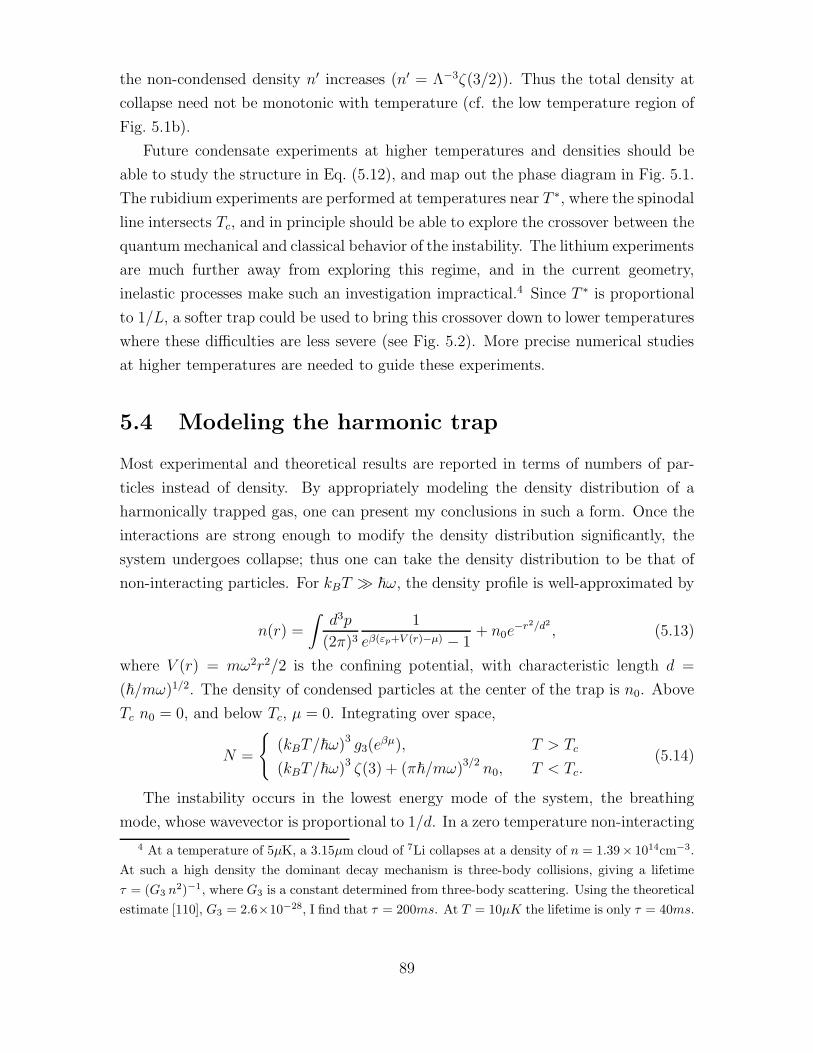
the non-condensed density n′ increases (n′ = Λ−3ζ(3/2)). Thus the total density at
collapse need not be monotonic with temperature (cf. the low temperature region of
Fig. 5.1b).
Future condensate experiments at higher temperatures and densities should be
able to study the structure in Eq. (5.12), and map out the phase diagram in Fig. 5.1.
The rubidium experiments are performed at temperatures near T ∗, where the spinodal
line intersects Tc, and in principle should be able to explore the crossover between the
quantum mechanical and classical behavior of the instability. The lithium experiments
are much further away from exploring this regime, and in the current geometry,
inelastic processes make such an investigation impractical.4 Since T ∗ is proportional
to 1/L, a softer trap could be used to bring this crossover down to lower temperatures
where these difficulties are less severe (see Fig. 5.2). More precise numerical studies
at higher temperatures are needed to guide these experiments.
5.4 Modeling the harmonic trap
Most experimental and theoretical results are reported in terms of numbers of par-
ticles instead of density. By appropriately modeling the density distribution of a
harmonically trapped gas, one can present my conclusions in such a form. Once the
interactions are strong enough to modify the density distribution significantly, the
system undergoes collapse; thus one can take the density distribution to be that of
non-interacting particles. For kBT ≫ ~ω, the density profile is well-approximated by
n(r) =
∫
d3p
(2π)3
1
eβ(εp+V (r)−µ) − 1+ n0e
−r2/d2
, (5.13)
where V (r) = mω2r2/2 is the confining potential, with characteristic length d =
(~/mω)1/2. The density of condensed particles at the center of the trap is n0. Above
Tc n0 = 0, and below Tc, µ = 0. Integrating over space,
N =
(kBT/~ω)3 g3(eβµ), T > Tc
(kBT/~ω)3 ζ(3) + (π~/mω)3/2 n0, T < Tc.(5.14)
The instability occurs in the lowest energy mode of the system, the breathing
mode, whose wavevector is proportional to 1/d. In a zero temperature non-interacting
4 At a temperature of 5µK, a 3.15µm cloud of 7Li collapses at a density of n = 1.39× 1014cm−3.
At such a high density the dominant decay mechanism is three-body collisions, giving a lifetime
τ = (G3 n2)−1, where G3 is a constant determined from three-body scattering. Using the theoretical
estimate [110], G3 = 2.6×10⁻²⁸, I find that τ = 200ms. At T = 10µK the lifetime is only τ = 40ms.
89

250
500
750
1000
1250
1500
Temperature [ µK]
2 4 6
N0( )max
20
40
60
80
100
120
N0( )max
Temperature [ nK]
10 20 30 40 50
a)
b)
Figure 5.3: Maximum number of condensed particles as a function of temperature,for the a) 7Li and b) 85Rb experiments. The (kΛT )0 terms in Eq. 5.9a have beenincluded in producing these plots, giving a slightly different shape than that quotedin Eq. (5.12).
90

gas the breathing mode has a density profile δρ ∝ (2r2/d2 − 3) exp (−r2/d2), where r
is the radial coordinate. In momentum space this distribution is peaked at wavevector
k = 2/d. At finite temperature thermal pressure increases the radius of the cloud and
the wavevector of the breathing mode becomes smaller. Since the response of the non-
condensed cloud is relatively insensitive to the wavevector, I look for an instability at
k = 2/d.
The resulting phase diagram, Fig. 5.4, is similar to that in Fig. 5.1. The most
significant difference is that the line of collapse follows the condensation line (on the
scale of the figure they appear to coincide over a significant temperature range). This
behavior can be understood by noting that for trapped particles, condensation results
in a huge increase in the central density of the cloud (a standard diagnostic of BEC).
5.5 Pairing
With minor changes the formalism presented here can be used to investigate the insta-
bility towards forming loosely bound dimers, or “pairs,” the Evans-Rashid transition.
Such an instability occurs in an electron gas at the superconducting BCS transition
[111], and has been predicted by Houbiers and Stoof [100, 112] to occur in the trapped
alkalis. The pairing is signalled by an instability in the T-matrix of the normal phase
[113], which plays the role that the density response function plays in the collapse.
Again, I simulate the finite size of the cloud by looking for an instability at k = 2π/L,
compared with k = 0 in a bulk sample. In analogy to Eq. (5.5), the T-matrix can be
written as a ladder sum,
T (k, ω) =g
1 − gΞ(k, ω). (5.15)
In this equation, k is the relative momentum of the pair. The instability towards
pairing is signalled by T → ∞, when gΞ = 1. To the same level of approximation as
Eq. (5.7a), the medium-dependent part of the “pair bubble” Ξ is
Ξ(k, ω) =
∫
d3q
(2π)3
f(q − k/2) + f(q + k/2)
~ω − (εq+k/2 + εq−k/2). (5.16)
Setting ω = 0, and expanding in small kλT (see appendix E.4.3), one finds
gΞ(k, ω = 0) = −4as
ΛT
[
4π
kΛTarctan
(
|ǫk/4µ|1/2
1 + |ǫk/4µ|1/2
)
(5.17)
+g1/2(eβµ) − |π/βµ|1/2 + O(kΛT )
]
.
91
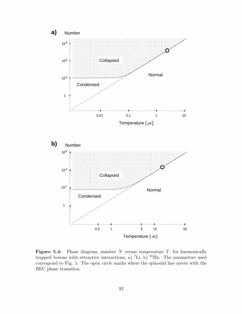
a)
b)
1 10
Temperature [ µK]
109
Normal
Condensed
103
106
0.1
Collapsed
Number
1
0.01
106
1
102
104
Number
Temperature [ nK]
1 105 500.5
Collapsed
CondensedNormal
Figure 5.4: Phase diagram, number N versus temperature T , for harmonicallytrapped bosons with attractive interactions; a) 7Li, b) 85Rb. The parameters usedcorrespond to Fig. 1. The open circle marks where the spinodal line meets with theBEC phase transition.
92

Except for the argument of the arctangent, this expression is identical to twice gχn0 as
given in Eq. (5.8). Since arctangent is a monotonic function, and its argument here is
smaller than in Eq. (5.8), one sees that gΞ < 2gχn0 , which implies that the instability
towards collapse occurs at a lower density than the pairing instability. Thus I conclude
that the pairing transition does not occur in an attractive Bose gas. Interestingly, in
the classical limit, the instabilities towards pairing and collapse coincide.
5.6 Domain formation in spinor condensates
The approach used here to discuss the collapse of a gas with attractive interactions
also describes domain formation in spinor condensates, and gives a qualitative un-
derstanding of experiments at MIT [9] in which optically trapped 23Na is placed in
a superposition of two spin states. Although all interactions in this system are re-
pulsive, the two different spin states repel each other more strongly than they repel
themselves, resulting in an effective attractive interaction. The collapse discussed
earlier becomes, in this case, an instability towards phase separation and domain for-
mation. The equilibrium domain structure is described in [114]. Here I focus on the
formation of metastable domains [115].
The ground state of sodium has hyperfine spin F = 1. In the experiments the
system is prepared so that only the states |1〉 = |F = 1, mF = 1〉 and |0〉 = |F =
1, mF = 0〉 enter the dynamics. The effective Hamiltonian is then
H =
∫
d3r∇ψ†
i · ∇ψi
2m+ V (r)ψ†
iψi +gij
2ψ†
iψ†jψjψi. (5.18)
where ψi (i = 0, 1) is the particle destruction operator for the state |i〉; summation
over repeated indices is assumed. The effective interactions, gij = 4π~2aij/m, are
related to the scattering amplitudes aF=0 and aF=2, corresponding to scattering in
the singlet (F1 + F2 = 0) and quintuplet (F1 + F2 = 2) channel, by [9, 114, 116]:
a ≡ a11 = a01 = a10 = aF=2, (5.19a)
δa ≡ a11 − a00 = (aF=2 − aF=0)/3. (5.19b)
Note that the |1〉+ |0〉 channel is purely F = 2 for identical bosons, since the F = 1
state is anti-symmetric and the scattering is purely s-wave. Numerically, a = 2.75nm
and δa = 0.19nm. In the equations of motion, these lengths appear as g = 4π~2a/m
and δg = 4π~2δa/m. Initially the condensate is static with density n = 1014cm−3,
and all particles in state |1〉. A radio-frequency pulse places half the atoms in the
93
|0〉 state without changing the density profile. Subsequently the two states phase
separate and form 40 ± 15 µm thick domains. The trap plays no role here, so I
neglect V (r) in Eq. (5.18) and consider a uniform cloud.
Within a mean field approximation, one writes ψi =√nm=ie
iφi, and the equa-
tions of motion for φi and nm=i are derived by making stationary the action S =∫
dt[∫
d3r (1/2i)(∂tψ∗ψ − ψ∗∂tψ) −H
]
, leading to a set of “hydrodynamic equa-
tions”,
∂tnm=i + ∇ · (nm=i∇φi) = 0 (5.20a)
∂tφi − (∇2√nm=i)/2m√nm=i + gijnm=j = 0, (5.20b)
the first of which is a continuity equation, and the second is analogous to Euler’s
equation for an ideal fluid. The initial stages of domain formation can be understood
by linearizing these equations about nm=0 = nm=1 = n/2. After eliminating the phase
variables, and Fourier transforming with respect to space and time,
(
ω2 − εk(εk + gn + δg n) −gnεk
−gnεk ω2 − εk(εk + gn)
)(
δnm=0
δnm=1
)
= 0. (5.21)
Here δnm=i = nm=i − n/2 is the fluctuation of the density of each species, and as
before εk = k2/2m. When δg is set to zero, the two solutions of these equations
represent a pure spin wave, where δnm=0 + δnm=1 = 0, or a pure density wave
where δnm=0 = δnm=1. For arbitrary δg, the spectrum of these modes become
ω2 = ε(
ε+ gn− δg n/2 ± [(gn)2 + (δg n/2)2]1/2)
, which for small δg is
~2ω2
ph =
(
~2k2
2m
)2
+ gn~
2k2
m+ O(δg), (5.22a)
~2ω2
sp =
(
~2k2
2m
)2
− δg n~
2k2
4m+ O((δg)2). (5.22b)
Similar excitation spectra were found in [117]. The subscripts ph or sp refer to the
phonon or spin-wave character of the excitations. Since δg > 0, the long-wavelength
spin excitations have imaginary frequencies. The mode with the largest imaginary
frequency grows most rapidly, and the width of the domains formed should be com-
parable to the wavelength λ of this mode. By minimizing Eq. (5.22b) one finds
λ =√
2π/n δa ∼ 20µm, in rough agreement with the observed domain size.
To connect these unstable modes to our previous discussion of the collapse more
explicitly, I note that in the mean field approximation, the interaction in Eq. (5.18)
is only a function of nm=0 and n, the density of particles in the state |0〉 and the total
94

density, respectively:
〈Hint〉 =
∫
d3r
(
g
2n2 − δg
2n2
m=0
)
, (5.23)
which shows explicitly the effective attractive interaction.
95

Chapter 6
Kinetic Theory
This Chapter develops the kinetic theory needed to describe a finite temperature gas
of Bose condensed atoms. The approach used here was developed in the 1960’s by
a series of authors, most notably Kadanoff and Baym [113] and Kadanoff and Kane
[118]. Recently several authors have applied these, or similar, ideas to trapped atomic
gases [119, 120, 121, 122, 123]. The underlying theory is complex, and the main goal
of most of these studies is to produce approximations that allow a real problem to be
solved.
In writing this Chapter I have three goals. First, and foremost, I want to develop
a formalism which can be applied to understanding a series of experimentally rele-
vant problems where both the coherent motion of the condensate and the incoherent
motion of the non-condensed particles play equal roles. These problems include the
dynamics of vortex decay, and the dynamics of domain formation in a spinor con-
densate. Second, with the aid of a small toy model, I would like to clarify how a
Bogoliubov quasiparticle differs from the collective condensate excitations with the
same dispersion. Finally, I would like to present a very compact derivation of the
kinetic equations which is of general interest.
The kinetic theory developed here is highly nontrivial. Readers may wish to
familiarize themselves with the material in Appendix E where a simpler linearized
theory is presented, and the material in Appendix C where response functions are
discussed.
6.1 Overview
In classical mechanics one describes the kinetics of a gas/liquid via a phase-space
distribution function f(R, p, T ), which measures the probability of having a particle of
96
momentum p at position R and time T . This distribution function obeys a Boltzmann
equation, typically of the form
(∂T + (p/m) · ∇R − (∇U) · ∇p)f = I[f ]. (6.1)
The left hand side of the Boltzmann equation describes the motion of the gas particles
if they were non-interacting; U is an arbitrary external field, m is the particle mass,
and ∇R and ∇p are gradients with respect to position and momentum variables.
The right hand side, the collision integral, describes the interactions between the
particles, and is a nonlinear function of f . The collision integral drives the system
towards equilibrium, and has the structure,
I[f ](R, p, T ) =∑
q
(Rq→p −Rp→q), (6.2)
where Rp→q is the total rate of particles scattering from momentum p to momentum
q. Classically, Rp→q is proportional to the number of particles in the state p, and so
one usually writes Rp→q = Γp→qf(q).
In a quantum theory one can derive a similar equation. The key is to recognize
that the single particle Green’s function G< = 〈ψ†(r1′, t1′)ψ(r1, t1)〉 behaves like a
phase space distribution. After writing G<(r1, t1, r1′, t1′) in terms of the center of
mass coordinates R = (r1 + r1′)/2 and T = (t1 + t1′)/2, and the relative coordinates
r = (r1−r1′) and r = (t1− t1′), one can Fourier transform with respect to the relative
coordinates,
G<(p, ω, R, T ) =
∫
d3r dt eiωt−ip·rG<(r, t;R, T ). (6.3)
If one integrates the resulting function over p, one gets the density of occupied states
in real space. Integrating over r, gives the density of occupied states in momentum
space. Thus G<(p, ω, R, T ) holds all of the physics that is contained in the classical
f(R, p, T ). In quantum mechanics, the energy of a particle ω is not independent of
its momentum p, requiring one to carry around an extra variable. When there is a
well-defined dispersion relationship, one can produce a quantum mechanical phase
space distribution function that is only a function of R, p, T .
Although I am interested in G<, it is a instructive to first understand the time
ordered Green’s function G = 〈T (ψ†ψ)〉. In a nonequilibrium (Schwinger-Keldysh)
formalism, the time ordering operator T , orders operators along a contour in the
complex time plane. This contour, illustrated in Fig. 6.1 begins at time t = −∞,
follows the real axis to t = +∞, returning to t = −∞ − iβ. Periodic boundary
conditions on this path ensure that the system is in thermal equilibrium at time
97

t
t = −∞− iβ
t = −∞ -
?
Figure 6.1: Contour in complex time used in the Schwinger-Keldysh formalism.
t = −∞. In all subsequent integrals, time integrals will implicitly follow this contour,
and space integrals will be over three dimensions. The equations for G take the form
of a convolution,∫
d2G−1(1, 2)G(2, 1′) = δ(1 − 1′). (6.4)
Here I have introduced the notational shorthand of using numbers to represent coor-
dinates, such as 1 represents r1, t1. In a normal system, after converting to relative
and center of mass (COM) coordinates, G−1 obeys the equation
G−1(p, ω, R, T ) = ω − p2/2m− V (R, T ) − Σ(R, T ; p, ω), (6.5)
which defines the self-energy Σ. Unfortunately the convolution in Eq. (6.4) is not
simple in term of the variables R, p, T, ω that describe the distribution function.
The Boltzmann equation only describes the evolution of the system close to equi-
librium in the presence of slowly varying disturbances. One can use this assumption
of slow variation to derive a “semi-classical” scheme for approximating the convolu-
tion. For pedagogical purposes I first show how this semiclassical method works in
an abstract setting. Let F be the convolution of two arbitrary functions A and B,
F (X, x) = A ∗B =
∫
dxA(x1, x)B(x, x1′), (6.6)
where x1 = X − x/2 and x1′ = X + x/2. By replacing x with the relative coordinate
r, one finds,
F (X, x) =
∫
dr A(RA = X + r/2, rA = x− r)B(RB = X + (r − x)/2, rB = r). (6.7)
In analogy to the expected behavior of the Green’s functions, suppose A and B are
peaked near rA = 0, and rB = 0, each falling off on a length scale ξ. Suppose
98

further that A and B vary only slowly as a function of their COM coordinates, with
a length scale L. Up to corrections of relative order ξ/L, the functions A and B can
be expanded to give
F (X, x) =
∫
dr A(X, x− r)B(X, r) + ∂XA(X, x− r)r
2B(X, r) (6.8)
−(x− r)
2A(X, x− r)∂XB(X, r) + · · ·
This expresses F as a series of terms, each of which is a convolution in the variable
x. The Fourier transform of F with respect to the relative coordinate is then
F (X, p) =
∫
dx e−ixpF (X, x) = A(X, p)B(X, p) +i
2∂XA∂pB − i
2∂pA∂xB. (6.9)
This convolution identity is the key to my derivation of the quantum Boltzmann
equation.
Turning back to the Green’s functions, the length scale over which the center of
mass of G changes is set by the external potential. This length is L. The rate of
change of the relative coordinate is set by the temperature and interactions. This
length scale, denoted ξ, is the coherence length. One builds Σ from G’s, and the
same length scales govern its behavior. Thus, as long as ξ ≪ L one can expand
the convolution for the equations of motion of G. (Similar arguments follow for the
convolution in the time domain.)
At this point it is convenient to introduce further notation. I define the Poisson
brackets A,B by
A,B = (∇RA · ∇PB −∇PA · ∇RB) − (∂TA∂ωB − ∂ωA∂TB). (6.10)
Then the convolution identity (6.9) is compactly written
A ∗B = AB + (i/2)A,B. (6.11)
Stepping back for a moment, the classical Boltzmann equation, Eq. (6.1), is described
by
ω − p2/2m− V (R, T ), f(R, p, T ) = I[f ]. (6.12)
Applying the convolution identity (6.11) to the equation for G,
(G−1 ∗G)(p, ω, R, T ) = 1 = (G−10 − Σ)G+
i
2(G−1
0 − Σ, G. (6.13)
Looking at a frequency ω → ω± iη, for small η, one can write this equation in terms
of its real and imaginary parts
G(ω ± iη) = Re[G(ω)] ∓ iA/2 (6.14a)
Σ(ω ± iη) = Re[Σ(ω)] ∓ iΓ/2. (6.14b)
99

This leaves four equations
(G−10 − Re[Σ])(Re[G]) + (Γ/2)(A/2) (6.15a)
± (Γ/4, Re[G] − (G−10 −Re[Σ]), A/4) = 1
(G−10 −Re[Σ])(A/2) − (Γ/2)(Re[G]) (6.15b)
± (Γ/4, Re[G] − (G−10 −Re[Σ]), A/4) = 0.
These are most transparent in the following form
(
G−10 −Re[Σ] Γ/2
−Γ/2 G−10 −Re[Σ]
)(
Re[G]
A/2
)
=
(
1
0
)
(6.16a)
Γ, Re[G] − (G−10 − Re[Σ]), A = 0. (6.16b)
The matrix is easily inverted to give the well-known results [113]
Re[G] = (G−10 −Re[Σ])/((G−1
0 − Re[Σ])2 + (Γ/2)2) (6.17a)
A = Γ/((G−10 − Re[Σ])2 + (Γ/2)2). (6.17b)
When Γ vanishes one must interpret the Lorentzian as a Dirac delta function.
We now have enough tools to investigate G<. The equations of motion for G<
can be derived from the equations for G, taking t1 < t1′ , in which case∫
d2 (G−10 (1, 2) − Σ(1, 2))G(2, 1′)
=
∫
d2G−10 (1, 2)G<(2, 1′) −
∫ t1
d21
iΣ>(1, 2)G<(2, 1′)
−∫ t1′
t1
d21
iΣ<(1, 2)G<(2, 1′) −
∫
t1′
d21
iΣ<(1, 2)G>(2, 1′) (6.18a)
=
∫
d2
[
G−10 (1, 2)G<(2, 1′) −
(
1
iΘ(1 − 2)[Σ>(1, 2) − Σ<(1, 2)]
)
G<(2, 1′)
+Σ<(1, 2)
(
1
iΘ(1′ − 2)[G>(2, 1′) −G<(2, 1′)]
)]
, (6.18b)
where Θ(x), the Heaviside step function, is zero for negative arguments and otherwise
equals 1. Since G−10 is strictly local in time one does not have to worry about breaking
the G−10 integrals up. Eq. (6.18b) is simple expressed in terms of retarded/advanced
response functions,
GA(12) =−1
iΘ(2 − 1)[G>(1, 2) −G<(1, 2)] (6.19a)
ΣR(12) =1
iΘ(1 − 2)[Σ>(1, 2) − Σ<(1, 2)], (6.19b)
100

in terms of which the equations of motion read,
(G−10 − ΣR) ∗G< − Σ< ∗GA = 0. (6.20)
Following the same procedure for t1 > t1′ , one finds
(G−10 − ΣR) ∗G> − Σ> ∗GA = 0. (6.21)
I now switch to center-of mass and relative coordinates, assuming L≫ ξ,
(G−10 − ΣR)G< − Σ<GA +
i
2((G−1
0 − ΣR), G< − Σ<, GA) = 0 (6.22)
As with the equations of motion for G, one can break this equation up into a real
and imaginary parts. Using the relations
GA(ω) = G(ω + iη) = ReG(ω) + iA(ω)/2 (6.23a)
ΣR(ω) = Σ(ω + iη) = ReΣ(ω) − iΓ(ω)/2; (6.23b)
one finds
Γ/4, G< − Σ<, A/4 = (G−10 −ReΣ)G< − Σ<ReG (6.24a)
(G−10 −ReΣ), G< − Σ<, ReG = −(ΓG< − Σ<A) (6.24b)
= −(Σ>G< − Σ<G>). (6.24c)
The last relationship appears as Eq. (9-30) in Kadanoff and Baym [113], and has the
structure of a Boltzmann equation [cf. (6.12)]; the left hand side contains streaming
terms, while the right is a collision integral. The functions Σ> and Σ< are the rates
of scattering out of and into a given chunk of phase space. The functions G< and G>
are the number of particles and the number of holes available in that chunk of phase
space.
When A is strongly peaked about a few discrete points, one can label those points
by a quantum number ν, and write A =∑
ν Aν . One then splits G< into a product
fνAν . The Poisson bracket obeys the Leibniz “product” rule, which for scalars reads
A,BC = A,BC + A,CB, and along with Eq. (6.16b), gives us,
(G−10 − ReΣ), fν
Aν+Γνf ν−Σ<, ReG+ReG, f νΓν = −(Γνfν−Σ<)Aν , (6.25)
where Γν is defined analogously to Aν . In equilibrium, Σ< = Γνf ν . Equation (6.24a)
forces A to be strongly peaked. See [113] for concrete examples that clarify this
structure.
101
6.2 Condensed system
6.2.1 Basic problems
In the condensed system, the Green’s function G< is a two-by-two matrix (cf. ap-
pendix C.4.1). However, for the weakly interacting system, the elementary excitations
are still quasiparticles, for which one should be able to find a Boltzmann equation.
There does not exist a one to one correspondence between particles and quasiparticles,
so the constraints imposed by number conservation have a different form in a con-
densed and noncondensed system. Matrix Green’s functions also appear in systems of
particles with internal degrees of freedom. The matrix structure arising from internal
degrees of freedom is simpler to deal with than the one arising from the presence of
a condensate.
In the last Section, all formulae which did not explicitly refer to real and imaginary
parts of functions are correct for more general matrix propegators (I was careful with
operator ordering). However one needs to take Hermitian and anti-Hermitian parts
of equations instead of real and imaginary. This is complicated by the fact that the
Hermitian and anti-Hermitian parts of the various matrices do not commute.
Since the different components do not commute, it is very hard to solve the re-
sulting equations. One might hope that one could formally manipulate the matrix
equations in the same manner as one does the scalar equations. Unfortunately the
basic assumptions underlying these manipulations only hold for scalar Green’s func-
tions. For example, the decomposition of G< into the product fA relies upon the
relationship A, f(A) = 0. This relationship is an obvious corollary of the chain rule
A, f(B) = A,Bf ′(B), along with A,A = 0. Unfortunately, neither the chain
rule, nor the latter identity are true for matrices. For example, consider the two by
two matrix A = ωτ1 + tτ2, for which the Poisson bracket reads A,A = 2iτ3 6= 0.
The most promising scheme to deal with these difficulties is to project the equa-
tions of motion onto Pauli matrices. This approach seems manageable, at least at the
mean field level. Instead of the two equations one has for the scalar case (one real,
one imaginary), one ends up with eight equations (four Pauli matrices, both real and
imaginary). In the next Section I investigate Bogoliubov theory in the context of this
formalism.
Alternatively one can make approximations which simplify the structure of the
matrix equations of motion. For example the Hartree-Fock approximation of Stoof et
al. [123], and the Popov approximation of Griffin et al. [120], each omit off-diagonal
terms in G−10 . For many problems such an approximation is appropriate.
102

6.3 Bogoliubov theory
In simple mean-field theories of the Bose gas (see appendix C.4.1), the inverse Green’s
function is of the form
G−1MF = G−1
0 − ΣMF = ωτ3 − ǫ− ∆τ1, (6.26)
where τν is a Pauli matrix, and the coefficients are generically calculated in some self-
consistent manner. In the simplest of these theories, the Bogoliubov approximation,
ǫ(R,P, T ) = p2/2m + gn0(R, T ), and ∆(R,P, T ) = gn0(R, T ). For the remainder of
this Section I neglect the subscripts MF . In a uniform, time independent system,
the spectral density is
A = 2πδ(G−1) = 2π [δ(ω −E) − δ(ω + E)]
[
ω
2Eτ3 +
ǫ
2E− ∆
2Eτ1
]
, (6.27)
= 2πδ(ω2 − E2) [ωτ3 + ǫ− ∆τ1] (6.28)
which can also be thought of as
A = 2πδ(ω − E)
(
u
v
)
(
u∗ v∗)
− 2πδ(ω + E)
(
v∗
u∗
)
(
v u)
, (6.29)
where the Bogoliubov factors are
u =
√
ǫ+ E
2E, (6.30a)
v = −√
ǫ−E
2E. (6.30b)
This representation of A is useful, along with the representation
G−1 = (ω −E)
(
u
−v
)
(
u∗ −v∗)
− (ω + E)
(
v∗
−u∗
)
(
v −u)
. (6.31)
For our purposes the representation in terms of Pauli matrices, Eq. (6.27) is easiest
to work with.
Now consider a slowly varying n0(R, T ). By construction G−1A = 0, but the
Poisson bracket is
G−1, A = ω2 − ǫ2 + ∆2, f/2 + τ1(ǫ,∆f − ∆, ǫf) (6.32)
+iτ2(∆, ωf − ω,∆f) + τ3(ω, ǫf − ǫ, ωf),
with f = 2πδ(ω2 − E2). The first term, proportional to the identity, is zero, but the
others are generically finite. Thus this spectral density does not obey the semiclassical
equations of motion.
103

The physical reason why this spectral density does not work is that it violates
number conservation. This violation occurs because as the spectrum changes, the
relationship between the number of quasiparticles and the number of real particles
changes. The collisionless Boltzmann equation conserves the number of quasiparticles,
so the spectral density has to be modified to take into account fluctuations in the
number of condensed particles.
To find the correct spectral density, I consider an arbitrary matrix of the form
A = a0 +∑
ν anτν . The equation
G−1, A = 2iG−1A, (6.33)
can then be broken up into eight components,
ω, a3 − ǫ, a0 − ∆, a1 = 0 (6.34a)
ǫ, a1 + ∆, a0 = −2ωa2 (6.34b)
ǫ, a2 = 2ωa1 + 2∆a3 (6.34c)
ǫ, a3 − ω, a0 = −2∆a2 (6.34d)
0 = ωa3 − ǫa0 − ∆a1 (6.34e)
ω, a2 = 2∆a0 + 2ǫa1 (6.34f)
∆, a3 + ω, a1 = −2ǫa2 (6.34g)
∆, a2 = 2ǫa3 − 2ωa0.. (6.34h)
Solving so many simultaneous partial differential equations is difficult. By combining
Eqs. (6.34f,6.34c,6.34h), one finds that a2 satisfies
ω2 − ǫ2 + ∆2, a2 = 0. (6.35)
Thus a2 is a function of ω2 − E2. The matrix element a2 is closely related to the
change in the number of quasiparticles. In equilibrium it vanishes.
These equations are amenable to a perturbative analysis where one formally treats
the Poisson brackets in (6.33) as small, which amounts to an expansion in powers of
ξ/L. Writing A =∑
ν A(ν), this analysis yields a hierarchy,
G−1A(0) = 0 (6.36)
G−1A(1) = −i/2G−1, A(0) (6.37)
G−1A(2) = −i/2G−1, A(1), (6.38)
and so on. As previously discussed, A(0) = 2πδ(ω2 − E2)[ωτ3 + ǫ − ∆τ1]. Iterating
these equations, and using the identity xδ‘(x) = −δ(x), one finds A(1) = −2πδ‘(ω2 −
104

E2)τ2(ǫ∆, ω + ωǫ,∆ + ∆ω, ǫ). These first order corrections have little effect
except to enforces particle conservation.
6.4 Response to a sudden change of interaction
strength
As a simple example to illustrate some of the issues raised by the kinetic approach
presented in this Chapter, I explore a uniform gas subjected to a sudden change
of interaction strength. In principle this situation could be experimentally realized
through the use of Feshbach resonances which allow the tuning of atomic interactions
[124]. I first study this problem using elementary means. I then use the machinery
developed in the preceding Sections to rederive these results.
6.4.1 The scenario
Before time t = 0 a uniform cloud of non-interacting bosons is in equilibrium. At
t = 0 interactions are suddenly turned on. The system is no longer in equilibrium,
and various excitations are generated. These excitations are generated on a timescale
of order the inverse mean field energy τMF ≈ ~/gn, where g = 4π~2as/m. These
excitations equilibrate on the collision time τc ≈ 1/(nσv). The times scale as different
powers of the scattering length; τMF ∼ 1/as, while τc ∼ 1/a2s. Thus one expects a
clear separation of timescales with τMF ≪ τc. Introducing typical parameters of Bose
gas experiments, τMF ≈ 0.6ms, and τc ≈ 17ms.
Due to this separation of timescales one can look at the two processes separately,
the generation of excitations and their equilibration. The former is described by a
collisionless (mean field) kinetic theory. There is a very interesting technical issue
here, in that within a collisionless kinetic theory, entropy is conserved and there
is no generation of quasiparticles. Thus these excitations are collective in nature
and represent an unusual oscillation of the condensate. Due to the presence of the
condensate, the spectrum of these collective oscillations is the same as the spectrum
of quasiparticle excitations.
105
6.4.2 Elementary approach
The mean field theory describing this situation can be derived from the Heisenberg
equations for the field operator Ψ,
(
i∂t +∇2
2m
)
Ψ = gΨ†ΨΨ. (6.39)
One writes Ψ = ψ+ ψ where ψ = 〈Ψ〉 is a c-number which represents the condensate,
and ψ is the operator that annihilates a non-condensed atom. Taking the expectation
value of Eq. (6.39) and keeping terms to quadratic order in the excitations, one arrives
at a non-linear Schrodinger equation
(
i∂t +∇2
2m
)
ψ = gψ∗ψψ + 2g〈ψ†ψ〉ψ + g〈ψψ〉ψ∗. (6.40)
Varying ψ in Eq. (6.40) gives
(
i∂t +∇2
2m
)
ψ = 2gψ∗ψψ + gψψψ†. (6.41)
where higher order terms have been ignored.
This approximation, a variant on the Bogoliubov approximation, obeys all of the
standard conservation laws (energy, mass, and current). These laws are easily verified
by noting that we could have derived the equations from functional differentiation of
a functional Φ (see Appendix D). In particular, multiplying Eq. (6.40) and (6.41)
by ψ∗ and ψ†, and subtracting the complex conjugate, gives ∂tn0 = −∂t〈ψ†ψ〉 =
2gIm(ψ∗)2〈ψψ〉, and verifies number conservation. Note that the standard Bogoliubov
theory, where the term g〈ψψ〉ψ∗ is ignored, does not conserve particle number.
In this formalism, a time and space dependent chemical potential is introduced as
the derivative of the condensates phase. One writes ψ =√n0 exp(iφ), and defines
vs ≡ (∇φ)/m (6.42)
µ ≡ −∂tφ−mv2s/2. (6.43)
Using these definitions, one rewrites Eq. (6.40) as a set of equations,
∂tn0 + ∇ · (n0vs) = 2gn0Im(〈ψψ〉e−2iφ) (6.44)
µ =∇2√n0
2m√no
+ g(n− n0) + gRe(〈ψψ〉e−2iφ). (6.45)
Equation (6.44) has the structure of a continuity equation. The right hand side repre-
sents the transfer of particles between the condensate and normal cloud. The second
106

line (6.45) is analogous to Euler’s equation for an ideal fluid. The term proportional
to ∇2√no is the “quantum pressure” term which played such an important role in
Chapter 5.
The equation for the non-condensed atoms is simplified by performing a Bogoli-
ubov transformation,
ψ = eiφ∑
k
[
eik·ruk(t)bk + e−ik·rv∗k(t)b†−k
]
, (6.46)
with c-number functions u and v and time independent boson operators bk and b†−k.
Since Eq. (6.41) is linear in ψ, this ansatz involves no further approximation. To
ensure the proper commutation relationships, one must enforce |uk|2−|vk|2 = 1. The
resulting equation for uk and vk is
(
i∂t − ǫk −gn0
−gn0 −i∂t − ǫk
)(
uk
vk
)
= 0. (6.47)
To the extent that one can ignore terms proportional to the depletion, the chemical
potential is µ = g(2n− n0), and ǫ = k2/2m+ gn0. In an inhomogeneous condensate
one would also need a term corresponding to spatial gradients, and also allow for the
presence of the superfluid velocity vs.
The stationary solutions to Eq. (6.47) correspond to (uk, vk) ∼ e±iEkt, where
E2k = ǫ2k − (gn0)
2. The physical, positive frequency solutions, are best characterized
by the bilinears (cf. 6.30),
|uk|2 =ǫ+ E
2E(6.48)
|vk|2 =ǫ− E
2E(6.49)
u∗kvk =−gn0
2E. (6.50)
More generically, Eq. (6.47) can be formally integrated,
(
uk(t)
vk(t)
)
= exp
[
it
(
−ǫk −gn0
gn0 ǫk
)](
uk(t = 0)
vk(t = 0)
)
. (6.51)
In this expression I have ignored the time dependence of n0 and vs, both assumed
to be slow and small. The exponential is simplified by noting that the square of its
argument is proportional to the identity, yielding,(
uk(t)
vk(t)
)
=
[
cos(Ekt) +i sin(Ekt)
Ek
(
−ǫk −gn0
gn0 ǫk
)](
uk(t = 0)
vk(t = 0)
)
. (6.52)
107

0.5 1 1.5 2tΤMF
0.2
0.4
0.6
0.8
1
n Ξ32Π2
Figure 6.2: Non-condensed density as a function of time after interactions are sud-denly turned on. The density is measured relative to its long-time value, and time ismeasured in terms of the mean field time.
It is readily verified that the constraint |uk|2 − |vk|2 = 1 is maintained by these
dynamics.
Focusing on the case at hand, at t ≤ 0, the system is in equilibrium with all of the
particles in the condensate. This implies that n0 = n and that 〈ψ†ψ〉 = 0. Using the
ansatz in Eq. (6.46), 〈ψ†ψ〉 =∑
k(v2k + (u2
k + v2k)〈b†kbk〉, which implies that bk|Ψ〉 = 0
and that vk = 0. The normalization condition u2k − v2
k = 1 then gives uk = 1.
From Eq. (6.52) the factor vk evolves as vk(t) = i(gn0/Ek) sin(Ekt). Thus the
number of excited particles n = 〈ψ†ψ〉 = V −1∑
k |vk|2 = V −1(gn0/Ek)2 sin2(Ekt).
At long times, the phase of the sine wave is essentially random, and one can replace
sin2(Ekt) with 1/2, giving n = V −1∑
k(gn0)2/2E2
k = 2π2/ξ3MF, where ξ2
MF = ~/gnm
is the condensate healing length. The time required to reach this asymptotic value is
of order τMF = ~/(gn0). The general integral analytically evaluates to
n(t) = 2π2/ξ3MF
(
1 − cosh(4t/τMF) + sinh(4t/τMF))
. (6.53)
This curve is shown in Fig. 6.2.
6.4.3 Further analysis
This model calculation seems quite simple, but the physics is actually quite strange.
For example, as anticipated, the number of quasiparticles, 〈b†kbk〉, is conserved. Thus
108

these oscillations of particles into and out of the condensate are somehow just a more
complicated oscillation of the condensate.
One gets further clues about this system by looking at the Green’s function,
G(1, 2) =1
i
⟨
T
[(
ψ1
ψ†1
)
(ψ†2 ψ2)
]⟩
, (6.54)
and the functions G< and G>, corresponding to the specific time orderings t1 < t2
and t1 > t2. To make contact to the material in the early part of this Chapter, I write
these functions in terms of the central coordinate T = (t1 + t2)/2 and the relative
coordinate t = t1 − t2.
In the example at hand, 〈b†b〉 = 0, thus
G>(1, 2) =
(
u(1)
v(1)
)
(u∗(2) v∗(2)) (6.55a)
G<(1, 2) =
(
v∗(1)
u∗(1)
)
(v(2) u(2)). (6.55b)
Using the expressions for u and v in Eq. (6.52),
G>(T,ω,k) = 2πδ(ω) gn
2E2
(
−gn cos(2EkT ) ǫ cos(2EkT )−iEk sin(2EkT )
ǫ cos(2EkT )−iEk sin(2EkT ) −gn cos(2EkT )
)
(6.56a)
+2πδ(ω−Ek) ǫ+E2E
(
ǫ+E2E
− gn2E
− gn2E
ǫ−E2E
)
+2πδ(ω+Ek) ǫ−E2E
(
ǫ−E2E
− gn2E
− gn2E
ǫ+E2E
)
G<(T,ω,k) = 2πδ(ω) gn
2E2
(
−gn cos(2EkT ) ǫ cos(2EkT )−iEk sin(2EkT )
ǫ cos(2EkT )−iEk sin(2EkT ) −gn cos(2EkT )
)
(6.56b)
+2πδ(ω−Ek) ǫ−E2E
0
B
@
ǫ+E2E
− gn2E
− gn2E
ǫ−E2E
1
C
A+2πδ(ω+Ek) ǫ+E
2E
0
B
@
ǫ−E2E
− gn2E
− gn2E
ǫ+E2E
1
C
A.
All of the dynamics occurs in the ω = 0 sector. This is a sign that these excitations
are actually deformations of the condensate. Subtracting the Green’s functions gives
A = G>−G< = 2πδ(ω−E)
(
ǫ+E2E
− gn2E
− gn2E
− ǫ−E2E
)
−2πδ(ω+E)
(
ǫ−E2E
− gn2E
− gn2E
− ǫ−E2E
)
, (6.57)
just as one finds in equilibrium. The spectral density A determines the dispersion and
wavefunctions of the quasiparticles. Since A is independent of time, the quasiparticles
are also unchanged in time. Because of the ω = 0 structure, G< andG> are not simply
proportional to A.
109
6.4.4 Kinetic approach
I now look at this problem in the language of the kinetic theory presented earlier in
this Chapter. In the absence of collisions, the fundamental equation is
G−10 − Σ, G< =
−2
i(G−1
0 − Σ)G<, (6.58)
where A,B = (∂ωA∂TB − ∂TA∂ωB) − (∇pA∇RB −∇RA∇PB).
Within this approximation,
(G−10 − Σ)(k, T, ω) = τ3ω − ǫk − gn0τ1, (6.59)
where ǫk = k2/2m + gn0, and n0 is taken to be independent of time. Since G< is
Hermitian, it can be decomposed in terms of Pauli matrices,
G< = g0 +∑
ν
gντν , (6.60)
where all of the g’s are real. Blindly substituting this decomposition into Eq. (6.58),
and using the relationship τµτν = δµ∋ + iǫµνλτλ, one finds the following six equations:
∂Tg3 = 0 (6.61a)
∂Tg2 = 2(ǫ)g1 + 2(gn0)g0 (6.61b)
∂Tg1 = −2ǫg2 (6.61c)
∂Tg0 = 2(gn0)g2 (6.61d)
0 = ωg3 − ǫg0 − (gn0)g1 (6.61e)
0 = ωg2 (6.61f)
0 = ωg1 + (gn0)g3 (6.61g)
0 = ωg0 − ǫg3, (6.61h)
which correspond to (6.34) specialized to the present case. The algebraic equations
can only be solved if the determinant vanishes,∣
∣
∣
∣
∣
∣
∣
∣
∣
∣
ω −gn0 −ǫω
gn0 ω
−ǫ ω
∣
∣
∣
∣
∣
∣
∣
∣
∣
∣
= ω2(ω2 − ǫ2 + (gn0)2) = 0, (6.62)
requiring ω = 0,±E. The distribution function will therefore have terms proportional
to δ(ω), δ(ω−E), and δ(ω+E). Considering each of these cases in turn, the Green’s
110

functions must have the general form,
G< = Aδ(ω − E)
(
ǫ− E −gn0
−gn0 ǫ+ E
)
+Bδ(ω + E)
(
ǫ+ E −gn0
−gn0 ǫ+ E
)
(6.63)
+δ(ω)
(
−gn0f1(t) ǫf1(t) + if2(t)
ǫf1(t) − if2(t) −gn0f1(t)
)
,
where A and B are constants, and f1 and f2 are functions of time. One also has
initial conditions∫
dω
2πG<(T = 0) = (1 − τ3)/2, (6.64)
which tells us that A − B = 2π/2E, f2(0) = 0, and f1(0) = (A + B)gn0/ǫ =
(A + B)ǫ/gn0 − 2π/gn0. Thus f1(0) = 2π(gn0/E2), A = 2π(ǫ + E)/2E2, and B =
2π(ǫ− E)/2E2.
The differential equations in Eq. (6.61) reduce to two equations,
∂T f2 = 2E2f1 (6.65)
∂T f1 = −2f2, (6.66)
which are trivially integrated. As expected one recovers Eq. (6.56b).
111
Chapter 7
Electromagnetically Induced
Transparency.
In this Chapter I describe the theory of electromagnetically induced transparency in
a gaseous medium, and show how this effect is used to stop light. Two formalisms
are discussed at length, a mean field theory, and an equilibrium Green’s function cal-
culation. I also say a few words about performing a non-equilibrium Green’s function
calculation, though a full analysis of such a theory goes beyond the scope of this
thesis.
7.1 Introduction: the basic picture
The New York Times writes “Scientists bring light to full stop” [125]. A light beam
is frozen in space. Is this the ultimate in delay lines? Will it be used for quantum
computing? Most importantly, how does it work?
The premise is simple. Light, which is a harmonic vibration of the electromagnetic
field, couples to polarons, harmonic vibrations of the polarization of a media – the
coupled excitation is referred to as a polariton. If one finds a scheme where one can
control the strength of the coupling, then one can adiabatically transform light into
a polarization wave. Polarons have very little dispersion, so the excitation is then
effectively stopped. At some later time one can transform the polaron back into a
photon, and light continues on its way.
It is useful to ask what is the simplest system in which one can perform this trick.
A first guess would be that one could use a cloud of two-level atoms. Unfortunately,
such a system is too simple, since there is no way to control the strength with which
light couples to the transition. Without being able to control the coupling strength,
112

one cannot adiabatically transfer the photon into a polaron. An even bigger problem
with two-level atoms is that since one has no control of the coupling to the electro-
magnetic field, one has to contend with spontaneous emission, and the polaron will
consequently have a very short lifetime.
The next level of sophistication is to use three-level atoms. Typically one considers
a Λ configuration, as portrayed in Fig. 7.1. The levels 1 and 2 represent different
hyperfine states of an atom, and there are no allowed transitions between them. The
state 3 is an excited electronic state, which couples to both 1 and 2, through different
polarizations of light, denoted α and β. There are three distinct polarization waves in
this system, depending upon which of the two states are coupled. The various cases
will be labeled by the symbols, P13, P12, P23. The goal will be to convert α photons
into P12 polarization waves. The switch which will turn on the coupling between the
photon and the polarization wave is a laser of β photons.
1
2
3α
β
Figure 7.1: Electronic structure of a 3-level atom in the Λ configuration. Levels 1and 3 are coupled by photons of polarization α, while levels 2 and 3 are coupled byphotons of polarization β
Suppose one has an intense laser of β photons. An atom in the 1 state, could
then absorb an α photon, jumping into the 3 state. Then the atom can be stimulated
to emit a β photon, dropping into the 2 state. Thus, when the laser is on, P12 is
coupled to the α photons. When the laser is off there is no coupling. This system
can therefore be used to stop light. This process is schematically shown in Fig. 7.2.
α3 2β
1
Figure 7.2: Schematic view of the transfer of a α photon into a P12 polarizationwave. An α photon comes along and excites an atom from the 1 state to the 3state, generating a P13 polaron. The excited atom emits a β photon, and changes thepolaron into a P12 polarization wave.
One caveat is needed. At no point in the procedure can the atom ever have a
113

probability of occupying the 3 state. The 3 state is highly excited and couples strongly
both α and β photons, consequently it has a relatively short lifetime. Any occupation
of this state will result in an absorption of photons. It is the lack of absorption which
gives this effect the name “electromagnetically induced transparency.”
It is also useful to say a few words about momentum conservation. If the initial
light beam has momentum k, and the coupling laser has momentum q, then the
polaron will have momentum k − q. An interesting twist on the experiment is to
convert the polaron back into a photon using a coupling beam of momentum q′ 6= q.
In this case the outcoming light will have momentum k − q + q′. This system could
then be used as a very efficient router, where light can be stored and the out-coupled
in an arbitrary direction.
7.2 A mathematical description of the system
The low energy physics of the light-atom system is given by the Hamiltonian,
H =∑
k
[
ck(α†kαk + β†
kβk) +∑
ν=1,2,3
(ǫk + Eν)ψ†νkψνk
]
(7.1)
+λ∑
kq
[
αqψ†3k+qψ1k + α†
qψ†1kψ3k+q + βqψ
†3k+qψ2k + β†
qψ†2kψ3k+q
]
+2π~
2as
m
∑
kqp
∑
µν
ψ†νkψ
†µpψµp−qψνk+q.
The first line gives the energies of the uncoupled modes. The photons of the two
polarizations are annihilated by the operators αk and βk. Atoms in the electronic
state ν with momentum k are annihilated by the operator ψνk. The atomic energy is
written as ǫk +Eν , where ǫk = k2/2m, and Eν is the energy of the electronic state ν.
The second line of this Hamiltonian gives the coupling between the photon modes
and the atomic transitions. The coupling constant λ is proportional to the dipole
matrix element for the electronic transition, explicitly
λ = −e〈1|x|3〉√
E3 −E1
2ǫ0V, (7.2)
Where 〈1|x|3〉 is the dipole matrix element, e is the electron charge, ǫ0 is the permi-
tivity of space, and V is the volume of space. I assume that the same λ can be used
for coupling states 3 and 2, as are used for 3 and 1. This approximation works well
for the current experiments, but generically two such constants are needed. One sees
114

in the Hamiltonian that the photons couple to polarization operators
Pij(q) =∑
k
ψ†ik+qψjk. (7.3)
Finally, the last line of the Hamiltonian gives the interaction between the atoms.
This interaction will only be important in that it will lead to some collisional broaden-
ing/decoherence. The collision cross-section is σ = 4πa2s. Some typical experimental
parameters are given in table 7.1.
Table 7.1: Experimental Parameters: temperature T , density n, collision rate 1/τc,natural width of state 3 Γ3, coupling constant λ, recoil energy Erecoil = k2/2m, and arate Γd associated with Doppler broadening (see Section 7.4)
87Rb (Phillips et al. [12]) 23Na (Liu et al. [11])
(E3 −E1)/2π~ 3.8 · 1014 Hz 5.1 · 1014Hz
(E2 −E1)/2π~ ∼ 105 Hz 1.8 · 109 Hz
kBT/2π~ 360K=7.5 · 1012 Hz 10−6 K=2 · 104 Hz
n 1011cm−3 1013 cm−3
as 5.8nm 4.9nm
1/τc 8.8 · 104 s−1 1.2 · 104s−1
Γ3 3.4 · 107s−1 6.1 · 107s−1
λ2V/~2 256 m3/s2 253 m3/s2
Erecoil/2π~ 3.6 · 104Hz 2 · 104 Hz
Γd =√ErecoilkBT/~ 5 · 108 Hz 2 · 104Hz√Nλ/~ 5.1 · 109 s−1 5.1 · 1010s−1
7.3 Mean field theory
There are two experiments which use an atomic gas to stop light. The group at
the Rowland Institute [11] uses a cloud of 23Na just above the BEC transition tem-
perature. The group at Harvard [12] uses a hot (360K) cloud of 87Rb. The former
experiment is almost in the regime where all components of the experiment are coher-
ent. The atoms are almost condensed, and all photon fields are generated by lasers.
The system can therefore be adequately described by a zero-temperature mean field
theory. Finite temperature effects are discussed in the following section.
First I restrict my attention to a single mode in each field, and ignore all incoherent
processes such as spontaneous emission and atomic collisions (these can be put back
115
in phenomenologically). Second, as the experiments are performed in very dilute
gases, I ignore the interactions between the atoms. Third, I ignore the dynamics of
the β field – this is assumed to be controlled by the experimenter by turning a dial.
With these assumptions, I write down the Heisenberg equations of motion for the
field operators, treating the operators as c-numbers,
i∂tψ1 = E1ψ1 + λα∗ψ3 (7.4a)
i∂tψ2 = E2ψ2 + λβ∗ψ3 (7.4b)
i∂tψ3 = E3ψ3 + λαψ1 + λβψ2 (7.4c)
i∂tα = ckα + λψ∗1ψ3. (7.4d)
The recoil energies have been absorbed into Eν . Two constants of motion are readily
verified,
n =∑
ν
|ψν |2 (7.5a)
n∗ = |α|2 + |ψ3|2 + |ψ2|2, (7.5b)
which are respectively the total density of atoms and the total density of “excitations.”
I now look for equilibrium solutions to these equations. I take β to be on resonance,
β(t) = βe−i(E3−E2)t, and rescale the frequencies of all the fields
ψi → e−iEitψi (7.6a)
α → e−iω0tα = e−i(E3−E1)tα. (7.6b)
The resonant frequency is ω0 = E3 −E1. After rescaling, the resulting equations are
i∂tψ1 = λα∗ψ3 (7.7a)
i∂tψ2 = λβ∗ψ3 (7.7b)
i∂tψ3 = λαψ1 + λβψ2 (7.7c)
i∂tα = (ck − ω0)α+ λψ∗1ψ3. (7.7d)
On resonance, ck = ω0; these equations are solved by αψ1 + βψ2 = 0 = ψ3, which
can be conveniently written as |α|2 = |β|2|ψ2|2/|ψ1|2. This state is known as a dark
polariton, since it does not undergo spontaneous emission. Utilizing the conservation
laws, one can relate |α|2 and |β|2 in this dark state via the equation,
|α|2 =|β|2(n∗ − |α|2)n− n∗ + |α|2 , (7.8)
116

ÈΒÈ20
n*
ÈΑÈ2
ÈΑÈ2=n*nÈΒÈ2
Figure 7.3: Relationship between probe and coupling beam intensity. The densityof probe photons |α|2 vs. the density of coupling photons |β|2, under the constraintthat the total number of excitations is held constant. As |β|2 → ∞ the densityof probe photons equals the total density of excitations n∗. If the coupling beam isadiabatically reduced, the probe photons are converted into polarons. When |β|2 → 0no probe photons remain. Asymptotically, |α|2 = (n∗/n)|β|2 as |β|2 → 0.
which is easily solved for |α|2,
|α|2 =1
2
√
(n− n∗ + |β|)2 + 4|β|2n∗ − (n− n∗ + |β|2). (7.9)
In particular, β → ∞, implies |α|2 → n∗, and the excitation is a photon. When
β → 0, the magnitude |α|2 → 0, and the excitation is a P12 polaron. At no point is
state 3 ever occupied. By adiabatically changing β one can tune from the photon to
the polaron. If n∗ ≪ n, one has a much more convenient expression
|α|2 =n∗|β|2n+ |β|2 . (7.10)
The full expression (7.9) is plotted in Fig. 7.3.
Experimentally, light is stopped by adiabatically ramping the strength of the
coupling laser. The experimentalist starts with a very strong β field. A laser of α
photons is incident on the atomic cloud. While the light is inside the cloud, the β
laser is slowly turned off, transforming the photons to polarons.
To understand the group velocity of the excitation one must look at the dispersion
ω(k). Technically, this starts to become tricky, since one has to solve Eq. (7.7) for
ck 6= ω0. To produce analytic results one has to expand in small parameters. For
117
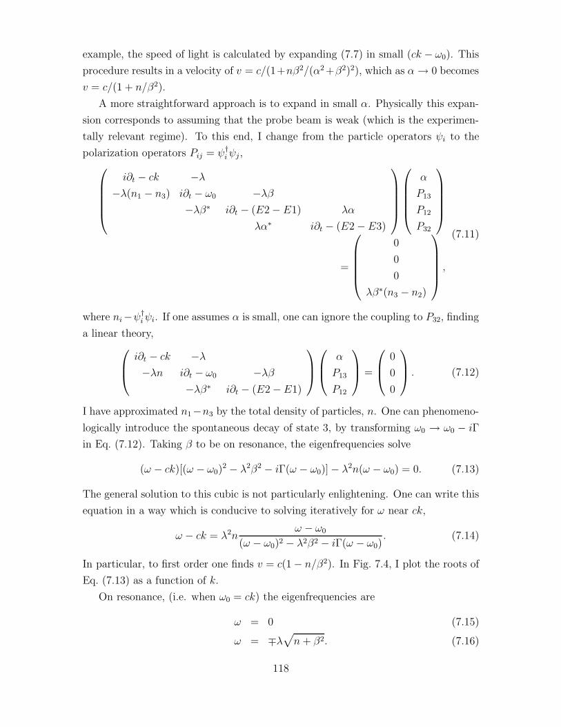
example, the speed of light is calculated by expanding (7.7) in small (ck − ω0). This
procedure results in a velocity of v = c/(1+nβ2/(α2 +β2)2), which as α → 0 becomes
v = c/(1 + n/β2).
A more straightforward approach is to expand in small α. Physically this expan-
sion corresponds to assuming that the probe beam is weak (which is the experimen-
tally relevant regime). To this end, I change from the particle operators ψi to the
polarization operators Pij = ψ†iψj ,
i∂t − ck −λ−λ(n1 − n3) i∂t − ω0 −λβ
−λβ∗ i∂t − (E2 − E1) λα
λα∗ i∂t − (E2 −E3)
α
P13
P12
P32
=
0
0
0
λβ∗(n3 − n2)
,
(7.11)
where ni−ψ†iψi. If one assumes α is small, one can ignore the coupling to P32, finding
a linear theory,
i∂t − ck −λ−λn i∂t − ω0 −λβ
−λβ∗ i∂t − (E2 −E1)
α
P13
P12
=
0
0
0
. (7.12)
I have approximated n1−n3 by the total density of particles, n. One can phenomeno-
logically introduce the spontaneous decay of state 3, by transforming ω0 → ω0 − iΓ
in Eq. (7.12). Taking β to be on resonance, the eigenfrequencies solve
(ω − ck)[(ω − ω0)2 − λ2β2 − iΓ(ω − ω0)] − λ2n(ω − ω0) = 0. (7.13)
The general solution to this cubic is not particularly enlightening. One can write this
equation in a way which is conducive to solving iteratively for ω near ck,
ω − ck = λ2nω − ω0
(ω − ω0)2 − λ2β2 − iΓ(ω − ω0). (7.14)
In particular, to first order one finds v = c(1 − n/β2). In Fig. 7.4, I plot the roots of
Eq. (7.13) as a function of k.
On resonance, (i.e. when ω0 = ck) the eigenfrequencies are
ω = 0 (7.15)
ω = ∓λ√
n + β2. (7.16)
118

Ω0
ck
Ω0-ÈΛΒÈ
Ω0+ÈΛΒÈ
Ω
Figure 7.4: Resonant frequencies of the mean-field equations. The dashed line showsthe frequencies when the coupling between the photons and the polarons are turnedoff.
On dimensional grounds, the adabaticity condition is that the rate of change of the
laser intensity is much less than the minimum energy spacing between the modes, i.e.
∂tβ
β≪ λ
√N
~. (7.17)
For alkali atoms, this ratio is of order 108 − 1010Hz.
Transparency
An important point here is that even in the presence of spontaneous emission from
state 3, the frequencies (7.15) and (7.16) are real, implying that there is no absorption.
In contrast, in the absence of the coupling beam, the α photons would be quickly
absorbed by the gas. This absorption results from generation of P13 excitations,
which have a very short lifetime.
7.4 Equilibrium Green’s functions
I now go beyond the mean field treatment by including various incoherent processes.
I use the standard finite temperature equilibrium Green’s functions as discussed in
Appendix C. The formalism can be conveniently built up starting from the equations
of motions for the field operators shown in Eq. (7.11). (This equation was presented
as a mean-field equation, but as long as one keeps the operators normal ordered
it is also true for the fields themselves.) I will however take a more intuitive, but
equivalent, approach of diagrammatically building up the self-energies for the photon
119
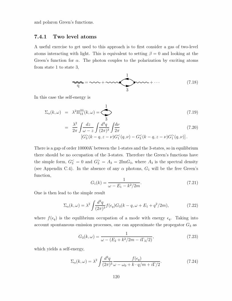
and polaron Green’s functions.
7.4.1 Two level atoms
A useful exercise to get used to this approach is to first consider a gas of two-level
atoms interacting with light. This is equivalent to setting β = 0 and looking at the
Green’s function for α. The photon couples to the polarization by exciting atoms
from state 1 to state 3,
q= +
3
1
+ · · · (7.18)
In this case the self-energy is
Σα(k, ω) = λ2Π(0)13 (k, ω) =
3
1
(7.19)
=λ2
2π
∫
dz
ω − z
∫
d3q
(2π)3
∫
dν
2π(7.20)
[G>3 (k − q, z − ν)G<
1 (q, ν) −G<3 (k − q, z − ν)G>
1 (q, ν)] .
There is a gap of order 10000K between the 1-states and the 3-states, so in equilibrium
there should be no occupation of the 3-states. Therefore the Green’s functions have
the simple form, G<3 = 0 and G>
3 = A3 = 2ImG3, where A3 is the spectral density
(see Appendix C.4). In the absence of any α photons, G1 will be the free Green’s
function,
G1(k) =1
ω −E1 − k2/2m. (7.21)
One is then lead to the simple result
Σα(k, ω) = λ2
∫
d3q
(2π)3f(ǫq)G3(k − q, ω + E1 + q2/2m), (7.22)
where f(ǫq) is the equilibrium occupation of a mode with energy ǫq. Taking into
account spontaneous emission processes, one can approximate the propegator G3 as
G3(k, ω) =1
ω − (E2 + k2/2m− iΓ3/2), (7.23)
which yields a self-energy,
Σα(k, ω) = λ2
∫
d3q
(2π)3
f(ǫq)
ω − ω0 + k · q/m+ iΓ/2. (7.24)
120
The resonant frequency is ω0 = E3 − E1 + Erecoil, where Erecoil = k2/2m.
There are two cases in which the integral is trivial to perform. First, at zero
temperature only the mode q = 0 is occupied, and
Σα(k, ω) =λ2n
ω − ω0 + iΓ/2, (7.25)
where n is the atomic density. The other simple case is when thermal broadening
dominates over the natural width Γ. Thermal broadening only dominates at quite
high temperatures, in which case one can take f to be a Boltzmann distribution, and
neglect Γ in Eq. (7.24). Using the identity (x− a)−1 = P (x− a)−1 ± iπδ(x− a), one
can read off the imaginary part of Σ,
ImΣα(k, ω) = −λ2n
2
( m
2πk2T
)1/2
exp(
− m
2k2T(ω − ω0)
2)
. (7.26)
The resonance clearly has a width Γd =√
4kBTǫk. The crossover between the zero
temperature behavior and the high temperature behavior occurs when Γd = Γ, which
is equivalent to kBT = Γ2/Erecoil.
For a Gaussian distribution one can perform the integral for all temperatures
without taking Γ → 0. The resulting line shape extrapolates between a Lorentzian
and a Gaussian (these two shapes are compared in Fig. 7.5). The basic trick involves
first integrating out the momenta perpendicular to k, the resulting one-dimensional
integral is of the form
I(x) =1√π
∫
dte−t2
t− x. (7.27)
Not surprisingly, this same integral plays an important role in the random phase
approximation to the density excitations of a gas of atoms discussed in Appendix E.
To evaluate the integral, one expresses (t− x)−1 as a Fourier integral
I(x) =i
π
∫ ∞
0
ds
∫ ∞
−∞dt exp
(
−t2 − is(t− x))
(7.28)
= ie−x2
(1 + erfix), (7.29)
where erf(x) is the error function. The end result is
Σα(k, ω) =λ2n
2
(
2
πΓ2d
)1/2
exp
(
−(ω − ω0 − iΓ/2)2
Γ2d
)
[ierf(i(ω − ω0 − iΓ/2)/Γd) − i] .
(7.30)
For further discussion of polaritons in gases of two level atoms, see [126].
121
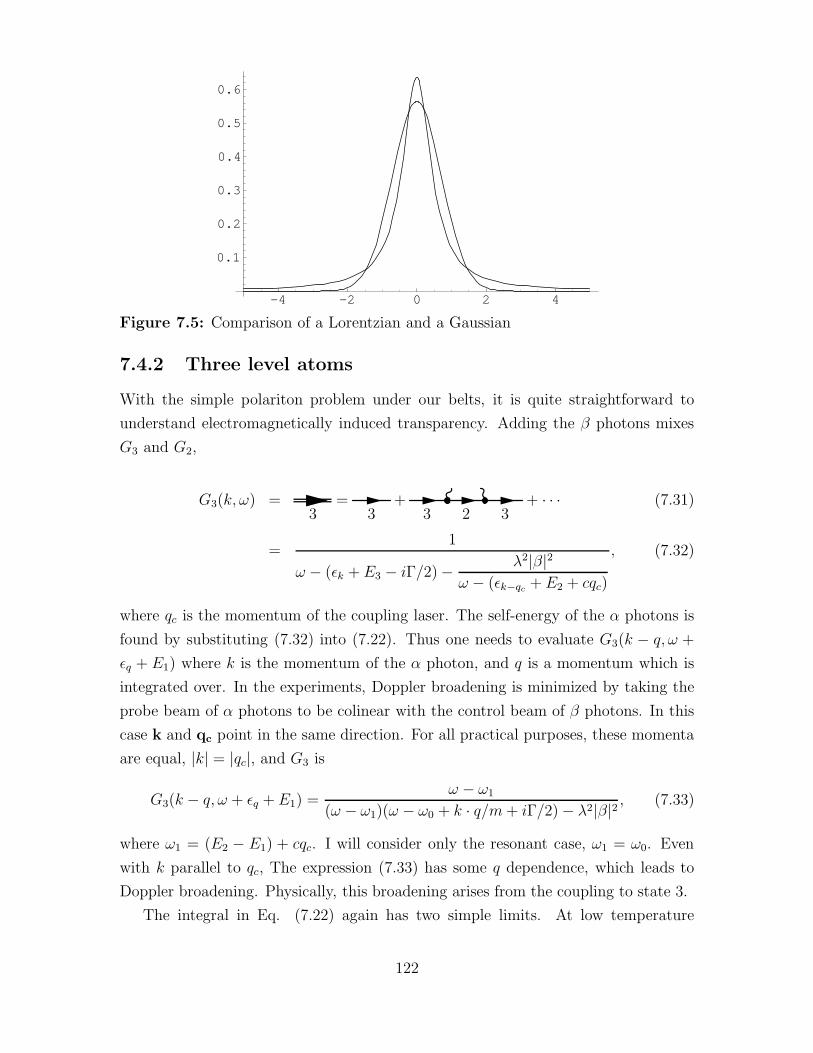
-4 -2 0 2 4
0.1
0.2
0.3
0.4
0.5
0.6
Figure 7.5: Comparison of a Lorentzian and a Gaussian
7.4.2 Three level atoms
With the simple polariton problem under our belts, it is quite straightforward to
understand electromagnetically induced transparency. Adding the β photons mixes
G3 and G2,
G3(k, ω) =3
=3
+3 2 3
+ · · · (7.31)
=1
ω − (ǫk + E3 − iΓ/2) − λ2|β|2ω − (ǫk−qc + E2 + cqc)
, (7.32)
where qc is the momentum of the coupling laser. The self-energy of the α photons is
found by substituting (7.32) into (7.22). Thus one needs to evaluate G3(k − q, ω +
ǫq + E1) where k is the momentum of the α photon, and q is a momentum which is
integrated over. In the experiments, Doppler broadening is minimized by taking the
probe beam of α photons to be colinear with the control beam of β photons. In this
case k and qc point in the same direction. For all practical purposes, these momenta
are equal, |k| = |qc|, and G3 is
G3(k − q, ω + ǫq + E1) =ω − ω1
(ω − ω1)(ω − ω0 + k · q/m+ iΓ/2) − λ2|β|2 , (7.33)
where ω1 = (E2 − E1) + cqc. I will consider only the resonant case, ω1 = ω0. Even
with k parallel to qc, The expression (7.33) has some q dependence, which leads to
Doppler broadening. Physically, this broadening arises from the coupling to state 3.
The integral in Eq. (7.22) again has two simple limits. At low temperature
122

(T ≪ Γ2/Erecoil),
Σα(q, ω) =λ2n(ω − ω0)
(ω − ω0)2 − λ2β2 + (ω − ω0)iΓ/2, (7.34)
while at high temperature
ImΣα(k, ω) = −λ2nmΛT
2kexp
(
− m
2k2T
[(ω − ω0)2 − λ2β2]2
(ω − ω0)2
)
. (7.35)
For arbitrary temperatures (treating f using Boltzmann statistics),
Σα(k, ω) = −λ2n
(
mΛT
2k
)
exp(−x2)(ierf(ix) − i) (7.36)
x =
(
βm
2k2
)1/2(ω − ω0)
2 − λ2β2 − iΓ(ω − ω0)/2
ω − ω0. (7.37)
The statement of transparency is that Im(Σα) = 0, which is true when ck = ω0.
I focus on zero temperature for a moment, where the photon propegator is
Gα =(ω − ω0)
2 − λ2β2 − iΓ(ω − ω0)/2
(ω − ck)[(ω − ω0)2 − λ2β2 − iΓ(ω − ω0)/2] − λ2n(ω − ω0), (7.38)
The denominator is familiar from the mean field theory in Section 7.3. The residues
at each of the poles tell how much of the excitation is a photon. The residue at
ω = ck = ω0 is
R = β2/(n+ β2). (7.39)
In the language of Section 7.3 this residue is the ratio |α|2/n∗ discussed in Eq. (7.10).
At finite temperature, the residue is
R = limω→ω0
(1 − Σ/(ω − ω0))−1, (7.40)
where Σ is given in Eq. (7.36). As z → ∞, the error function asymptotically behaves
as
erf(iz) ∼ exp(z2)/√πz, (7.41)
which yields the same residue. One could have guessed that the residue is temperature
independent. The only way that temperature could affect this state is through the
Doppler shift of the atomic transitions. These shifts exactly cancel on resonance,
resulting in a temperature independent residue.
123

7.5 Non-equilibrium Green’s functions
For completeness, here I make a few notes about going beyond the equilibrium theory
discussed in Section 7.4. This non-equilibrium theory is a topic I would like to address
in the future.
The full kinetic theory can be discussed in terms of the matrix Green’s function,
G =1
i
λα†α λP †13α λP †
12α
λα†P13 λP †13P13 λP †
12P13
λα†P12 λP †13P12 λP †
12P12
. (7.42)
The equations of motion for the Green’s function is formally written as G−1G = 1.
At zero temperature, where ψ1 is a c-number,
G−1 =
i∂t − ck −λ 0
−λ (i∂t − ω0 + iΓ/2)/n −λβ/n0 −λβ∗/n (i∂t − ω0)/n
(7.43)
I have explicitly taken β to be on resonance, and have neglected the dispersion of the
polarons. This expression is nothing but the equations of motion in Eq. (7.12). For
time independent β, these equations are easily integrated to reproduce the results of
the equilibrium theory. To describe a non-equilibrium theory, one can perform the
Wigner transform outlined in Chapter 6. In general, the resulting equations need to
be solved numerically, and its analysis is a topic of further research.
124

Chapter 8
Summary
Experiments on cold atomic clouds have demonstrated a diverse and extremely in-
teresting set of phenomena. In this thesis I provided a theoretical description of a
subset of these phenomena. I derived the effect of interactions on the phase tran-
sition temperature of a Bose gas. I calculated the lifetime of persistent currents in
toroidal traps. I produced a phase diagram which describes the stability of a cloud of
bosons with attractive interactions. I presented a kinetic theory for describing finite
temperature clouds of degenerate particles. I explored the interaction of light with
atomic clouds, providing a theoretical basis for experiments in which light is brought
to a halt.
125

Appendix A
Mathematical Functions
A.1 The polylogarithm functions
This appendix is intended as a reference for the properties of the polylogarithm func-
tions. Further details can be found in [127, 128, 129, 130].
The polylogarithm functions are defined by the series
gν(z) =∞∑
j=1
zj
jν. (A.1)
Analytically, they possess a singularity at z = 1, typically a logarithmic branch point.
For ν > 1 the limit z → 1 of gν(z) is well defined and is equal to ζ(ν).
The polylogarithm functions obey the relationship
zd
dzgν(z) =
d
d log zgν(z) = gν−1(z). (A.2)
This relationship, plus the closed form
go(z) =z
1 − z, (A.3)
allows one to calculate many of the properties of the polylogarithm functions for
integral ν. In particular one can use this relationship to calculate an asymptotic
expansion of gν(e−x) for small x. For this expansion I introduce the Bernoulli numbers
Bn, defined by the generating function
∑
n
Bnxn
n!=
x
ex − 1= x go(e
−x). (A.4)
These numbers are tabulated in table A.1, and can be related to the Riemann zeta
function via
Bn = (−1)nn ζ(1 − n) n = 1, 2, . . . (A.5)
126

Integrating (A.4) one finds
gν(e−x) =
(−x)ν−1
(ν − 1)!
[
− log x+
ν−1∑
m=1
1
m
]
+
∞∑
k=0k 6=ν−1
ζ(ν − k)(−x)k
k!. ν = 1, 2, 3, . . .
(A.6)
The equivalent expression for non-integral ν is
gν(e−x) = Γ(1 − ν)xν−1 +
∞∑
k=0
ζ(ν − k)(−x)k
k!, ν 6= 1, 2, 3, . . . (A.7)
One derives this latter expression by taking the Mellin-Barnes transform of gν(e−x)
[131]. A form of Laplace transform, the Mellin transform of a function f(x) is a
function F (s), related to the original by
F (s) =
∫
dx xs−1f(x) (A.8a)
f(x) =1
2πi
∫ c+i∞
c−i∞ds xs−1F (s), (A.8b)
where the contour in the inverse transform must be taken to the right of all the
singularities of F (s). In practice the latter integral is performed via the residue
theorem.
The Mellin transform of gν is
Gν(s) =
∫ ∞
0
gν(e−x)xs−1dx = ζ(ν + s)Γ(s). (A.9)
Gν(s) is well defined for large enough s. One inverts the transform via a contour
integral
gν(e−x) =
1
2πi
∫ c+i∞
c−i∞Gν(s)x
−sds, (A.10)
where the contour is to the right of all singularities of Gν(s). This integral is then
evaluated using the residue theorem along with the following facts. 1) The function
Table A.1: Bernoulli numbers Bn, as defined by the generating functiont
et − 1=
∑
n
Bntn
n!.
B0 B1 B2 B3 B4 B5 B6 B7 B8
1 −12
16
0 − 130
0 142
0 − 130
127

ζ(s) is regular, except at s = 1 where it has a pole with residue 1. 2) The function
Γ(s) is regular except when s is a non-positive integer. The residue of Γ(s) at s = −nis (−1)n/n!. Summing over the residues gives equation (A.7).
128
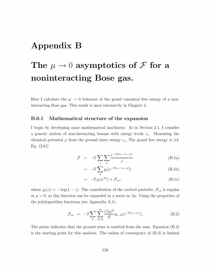
Appendix B
The µ→ 0 asymptotics of F for a
noninteracting Bose gas.
Here I calculate the µ → 0 behavior of the grand canonical free energy of a non-
interacting Bose gas. This result is used extensively in Chapter 2.
B.0.1 Mathematical structure of the expansion
I begin by developing some mathematical machinery. As in Section 2.1, I consider
a generic system of non-interacting bosons with energy levels εi. Measuring the
chemical potential µ from the ground state energy εo, The grand free energy is (cf.
Eq. (2.6))
F = −T∑
j
∑
n
e−βj(εn−εo−µ)
j(B.1a)
= −T∑
n
g1(e−β(εn−εo−µ)) (B.1b)
= −Tg1(eβµ) + Fex, (B.1c)
where g1(z) = − log(1 − z). The contribution of the excited particles, Fex is regular
at µ = 0, so this function can be expanded in a series in βµ. Using the properties of
the polylogarithm functions (see Appendix A.1),
Fex = −T∑
n
′ ∞∑
k=0
(βµ)k
k!g1−k(e
−β(εn−εo)). (B.2)
The prime indicates that the ground state is omitted from the sum. Equation (B.2)
is the starting point for this analysis. The radius of convergence of (B.2) is limited
129

by the pole at µ = ε1 − εo. The coefficients of βµ in Eq. (B.2),
fk =∑
n
′g1−k(e
−β(εn−εo)), (B.3)
are thermodynamic derivatives of the free energy with respect to the chemical poten-
tial, evaluated at µ = 0. Hence they give the moments (in fact the cumulants) of the
number of excited particles at temperatures below Tc. In particular:
< Nex > = f1 (B.4a)
< δN2ex > = 〈N2
ex〉 − 〈Nex〉2 = f2. (B.4b)
I proceed by expanding fk in powers of the inverse temperature β. The structure
of the expansion is understood by writing
fk =
∫
dE ρex(E) g1−k(eβE) (B.5a)
≈∫
dEρex(E)
(βE)k+ O(βk−1). (B.5b)
where ρex(E) is the density of excited states. For low enough energies the density
of states has the form ρ(E) ∼ Eα/γα+1, where γ has the dimension of energy. If
k < α + 1 the integral converges and fk ∼ (kBT/γ)α+1. Otherwise, the sum is
infrared divergent, and will be dominated by the first term. On dimensional grounds
the lowest energy state has energy ε1 ∼ γ, so in this latter case fk ∼ (kBT/γ)k.
To make these results more concrete, briefly consider point particles in a three
dimensional box, where α = 1/2 and γ ∼ ~2/mL2. According to this argument, the
number of excited particles is extensive, Nex = f1 ∼ L3, while the fluctuations are
anomalously large 〈δN2ex〉 = f2 ∼ L4. These large fluctuations in the number of non-
condensed particles are related to the large fluctuations in the number of condensed
particles (2.25).
B.0.2 The Mellin-Barnes Transform
To go beyond these order-of-magnitude estimates of fk, one performs a Mellin-Barnes
transform defined in equation (A.9). This transform allows one to express fk as a
sum of power-laws.
To produce an expansion of fk in powers of β, one should take the Mellin transform
of (B.3) with respect to β. This approach is inconvenient, since β is a dimensional
quantity. Instead I introduce a dummy variable x multiplying β, then in the end one
130

can set x = 1. Thus I define
Fk(s) =
∫
dx xs−1∑
n
′g1−k(e
−xβ(εn−εo)) (B.6a)
=∑
n
′∑
j
1
j1−k
∫
dx xs−1e−xβj(εn−εo) (B.6b)
= ζ(s+ 1 − k)Γ(s)∑
n
′(
1
β(εn − εo)
)s
. (B.6c)
The rightmost pole of Fk(s) gives the leading order behavior of fk as β → 0. The
zeta-function has a pole at pole at s = k with residue 1. the Gamma function has
poles at s = −m (m=0,1,2,. . . ) with residue (−1)m/m!. The remainder, designated
the spectral zeta function
Z(s) =∑
n
′(
1
β(εn − εo)
)s
, (B.7)
contains all the information about the details of the system.
We now have a simple algorithm for finding the expansion of F . First one finds
the poles of Z(s), giving all of the singularities of Fk(s). Assuming one only have to
deal with isolated singularities (as is the case), it is a simple matter to directly write
down fk, since fk is identically equal to the sum of the residues of Fk(s),
fk =∑
poles si
ResFk(s), si. (B.8)
In the following two Sections I specialize first to particles in a d-dimensional box,
then to particles in a harmonic well.
B.0.3 Particles in a Box
The spectral zeta function for particles in a box, with dispersion
ε = (~2/2mℓ2)(n2x + n2
y + · · · ), (B.9)
is discussed by Ziff et al. [127]. Following those authors, I introduce sums Cd(s) given
by
Cd(s) =Γ(s)
πs
∑′
nx,ny,...
1
(n2x + n2
y + · · · )s, (B.10)
in terms of which the spectral zeta function is
Γ(s)Z(s) =
(
L
λ
)2s
Cd(s). (B.11)
131

Some sample values of the sums Cd(s) are given in Table B.1. The function Cd(s) is
regular except for poles at s = d/2 and s = 0, where the residues are respectively 1
and −1. These singularities can be removed to produce an analytic function
Cd(s) = Cd(s) +1
s− 1
s− d/2− 1
d/2. (B.12)
It will only be necessary to evaluate this function at s = 0 or s = d/2, where it is
equal to the regular part of Cd(s). The function Cd(s) is tabulated in Table B.2.
Putting together the poles from Z(s) and from the zeta function in (B.6c), one
finds that for k 6= 0, d/2,
fk =
(
ℓ
Λ
)d
ζ(1 − d/2 − k) +
(
ℓ
Λ
)2k
Cd(k) − ζ(1 − k), (B.13a)
while for even d,
fd/2 =
(
ℓ
Λ
)d(
2 logℓ
Λ+ γ + Cd(d/2)
)
, (B.13b)
and for k = 0,
f0 = −2 logℓ
Λ− γ + Cd(0). (B.13c)
In the latter two equations γ ≈ 0.577216 is Euler’s gamma, which appears here
because ζ(s) = 1s−1
+ γ + O(s− 1).
B.0.4 Harmonic Well
The harmonic well, with ε = ~Ω(n1 + · · ·+nd +d/2) is slightly easier to analyze than
the uniform gas since the energy levels are evenly spaced. The spectral zeta function
for a harmonically trapped gas is
Z(s) = (β~ω)−s∑
nx,ny,...
(
1
nx + ny + · · ·
)s
, (B.14a)
= (β~ω)−sQd(s), (B.14b)
where the sum is taken over all non-negative n, where not all of the n’s are zero. The
sum Qd(s) can be written as
Qd(s) =∑
n
g(d)n
ns, (B.15)
132
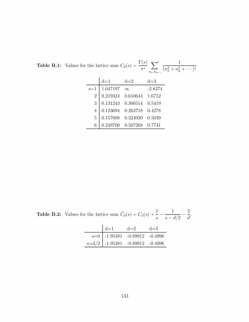
Table B.1: Values for the lattice sum Cd(s) =Γ(s)
πs
∑′
nx,ny,...
1
(n2x + n2
y + · · · )s
d=1 d=2 d=3
s=1 1.047197 ∞ -2.8374
2 0.219324 0.610644 1.6752
3 0.131243 0.300514 0.5419
4 0.123694 0.263718 0.4278
5 0.157008 0.324039 0.5039
6 0.249700 0.507268 0.7741
Table B.2: Values for the lattice sum Cd(s) = Cd(s) +1
s− 1
s− d/2− 2
d.
d=1 d=2 d=3
s=0 -1.95381 -0.89912 -0.4996
s=d/2 -1.95381 -0.89912 -0.4996
133

where g(d)n is the number of ways of adding d non-negative numbers together to form
the number n. Calculating g(d)n is a famous boson counting problem,1 and g
(d)n can be
written in terms of a binomial coefficient,
g(d)n =
(
n+ d− 1
d− 1
)
. (B.16)
The binomial coefficients(
nm
)
, read “n choose m,” give the number of ways of taking
m objects out of a set of n, disregarding order. I now expand this in powers of n as
g(d)n =
1
Γ(d)
∑
k
[
d
k
]
nk−1. (B.17)
The Stirling numbers of the second kind[
nm
]
, read “n cycle m”, give the number of
ways of making m cycles of n objects. Table B.3 lists some of Stirling numbers. Note
that[
nn
]
= 1.
Qd(s) can now be written as
Qd(s) =∞∑
n=1
g(d)n
1
ns(B.18a)
=∑
j
1
Γ(d)
[
d
d− j
]
ζ(s+ 1 − d+ j), (B.18b)
with poles at s = d, d − 1, . . . , 1. I tabulate Qd(s) in Table B.4. Since there are so
many poles, the full expression for fk is rather daunting. The leading order behavior
is
fk =
(β~ω)−dζ(d+ 1 − k), k < d
(β~ω)−d(
∑
l 6=0
[
dd−l
]
ζ(1 + ℓ) + Γ(d) (− log(β~ω) − γ +Hd−1))
, k = d
(β~ω)−kΓ(k)Qd(k), k > d,
(B.19)
where Hn =∑n
m=11m
is the partial sum of reciprocals. Including higher order terms
1 The standard counting argument goes as follows. The number of ways of writing n as a sum of
d non-negative numbers is the same as the number of ways of writing n + d as a sum on d positive
numbers. The latter is calculated by writing down n tick marks, and asking how many ways are
there to put d − 1 barriers in the n + d − 1 spaces between the tick marks. This gives
g(d)n =
(
n + d − 1
d − 1
)
.
134

Table B.3: Stirling numbers of the second kind[
nm
]
m=0 1 2 3 4 5
n=0 1
1 0 1
2 0 1 1
3 0 2 3 1
4 0 6 11 6 1
5 0 24 50 35 10 1
6 0 120 274 225 85 15
Table B.4: Values for the lattice sum Qd(s) =∑
nx,ny,...
(
1
nx + ny + · · ·
)s
.
d=1 d=2 d=3 d=4 d=5
s=1 ∞ ∞ ∞ ∞ ∞2 1.64493 ∞ ∞ ∞ ∞3 1.20206 2.84699 ∞ ∞ ∞4 1.08232 2.28438 3.70788 ∞ ∞5 1.03693 2.11925 3.26144 4.4974 ∞6 1.01734 2.05427 3.1139 4.20104 5.32539
135

gives
fk =d−1∑
j=0
j 6=d−k
(β~ω)j−dΓ(d− j)
Γ(d)
[
d
d− j
]
ζ(d+ 1 − k − j) (B.20)
+(β~ω)−kΥk +∑
n
(β~ω)nζ(−n− k + 1)(−1)n
n!Qd(−n).
Where the contribution Υk is given by
Υk =
Q′d(0) −Qd(0) log β~ω , k = 0
(Γ(k)/Γ(d))∑
l 6=d−k
[
dd−l
]
ζ(k + 1 − d+ l)
+Γ(k) (− log(β~ω) − γ +Hk−1), 0 < k ≤ d
Γ(k)Qd(k) , k > d
(B.21)
I tabulate Q′d(0), the derivative of Qd(s), in Table B.5.
Table B.5: Derivative of (the analytic continuation of) the lattice sum Q′d(0).
Q′1(0) Q′
2(0) Q′3(0) Q′
4(0) Q′5(0)
-0.918939 -1.08436 -1.18229 -1.25176 -1.3054
136

Appendix C
Review of response functions
C.1 Introduction
Green’s functions, and more general response functions, play an important role in
this thesis. In this Appendix I review the concepts and techniques which are used in
the rest of the thesis. In general my notation follows Kadanoff and Baym [113].
C.2 Linear response theory
Linear response theory is the general study of the response of a system to a weak
probe. Because the probe is weak, it does not perturb the system. As a concrete
example, let us consider the response of a resistor to an applied current. The re-
sponse is quantified by measuring the voltage across the resistor. For weak enough
currents, the voltage is proportional to the current. The impedance, Z = ∂V/∂I, is
the coefficient of proportionality.
The general framework in which one introduces linear response theory is to write
the perturbation in the form
Hpert(t) = α(t)A, (C.1)
where A is the operator that the perturbation couples to (in our example A would
be the voltage across the sample, since the energy is IV ), and α(t) is a c-number
describing the time dependence of the perturbation. One then looks at the time
dependence of some other operator, B, which within the interaction picture is
B(t) = 〈T(
eiR t
−∞dτ V (τ)
)
B T(
e−iR t
−∞dτ V (τ)
)
〉. (C.2)
In the interaction picture, the perturbation Hpert(t) appears in the form
V (t) = eiH0(t)Hpert(t)e−iH0(t). (C.3)
137

To find the linear response, one expands the exponentials to first order in α,
δB(t) =
∫ t
−∞dτ α(τ)
1
i〈[B(t), A(τ)]〉, (C.4)
=
∫ ∞
−∞dτ α(τ)χr
BA(t− τ), (C.5)
which defines the retarded response function
χrBA(t) = θ(t)
1
i〈[B(t), A(0)]〉. (C.6)
In the frequency domain, the response is particularly simple
δB(ω) = α(ω)χrBA(ω). (C.7)
Thus our whole task is to calculate χrBA(ω).
The easiest route to calculating χrBA leads one through the complex frequency
plane. This detour is not surprising, since one often uses complex analysis to calculate
Fourier transforms. One needs two expressions to continue. First, one needs the well
known convolution identity
∫
dt eiωtf(t)g(t) =
∫
dt eiωt
∫
dν
2πe−iνt
∫
dν ′
2πe−iν′tf(ν)g(ν ′) (C.8)
=
∫
dν
2πf(ν)g(ω − ν). (C.9)
The second expression one needs is the Fourier transform of a theta function
∫
dteiωtθ(t)e−ηt =−1
iω − η=
i
ω + iη(C.10)
∫
dteiωtθ(−t)eηt =1
iω + η=
−iω − iη
. (C.11)
To ensure convergence of the integrals, I have introduced an exponential that decays
on a timescale 1/η. At the end of the calculation I will take η to zero.
Using these simple expressions one finds
χrBA(ω) =
∫
dω′
2π
χ[B,A](ω)
ω − ω′ + iη, (C.12)
where
χ[B,A](ω) =
∫
dt eiωt〈[B(t), A(0)]〉 (C.13)
= −2 ImχrBA(ω). (C.14)
138

The last equality is seen by using the identity
1
ω − ω′ + iη= P
1
ω − ω′ − iπδ(ω − ω′) (C.15)
which is easily proven by contour integration. Equation (C.14) only holds when ω is
real.
There are very efficient techniques to calculate χ[B,A](ω). These make use of the
time ordered response function
χBA(t) =1
i〈T (A(0)B(t))〉, (C.16)
which is closely associated with
χ>BA(t) = 〈B(t)A(0)〉, (C.17)
χ<BA(t) = 〈A(0)B(t)〉. (C.18)
In the frequency plane, the time ordered response function is
χBA(ω) =
∫
dt eiωt 1
i(θ(t)χ>
BA(t) + θ(−t)χ<AB(t)) (C.19)
=
∫
dω′
2π
χ[B,A](ω′)
ω − ω′ . (C.20)
The retarded and time-ordered response functions are simply related,
χrBA(ω) = χBA(ω + iη). (C.21)
Most manipulations of the time-ordered functions take advantage of the fact that
they are periodic in imaginary time. The basic argument is that this periodicity
follows from the cyclical invariance of the trace,
〈B(t)A(0)〉 = Tr
e−β(H−µN)[
eiHtB(0)e−iHt]
A(0)
(C.22)
= Tr
e−β(H−µN)[
eβ(H−µN)e−iHtA(0)eiHte−β(H−µN)]
B(0)
(C.23)
= 〈A(−(t+ iβ))B(0)〉 (C.24)
= 〈A(0)B(t+ iβ)〉. (C.25)
The end expression will look slightly different if A does not commute with N . Further
complications arise when one is dealing with Fermi operators, but for our purposes
these can be ignored. By convention one defines time ordering so that t = −iβ is
later than t = 0. Thus
χBA(t = 0) = χBA(t = −iβ). (C.26)
139
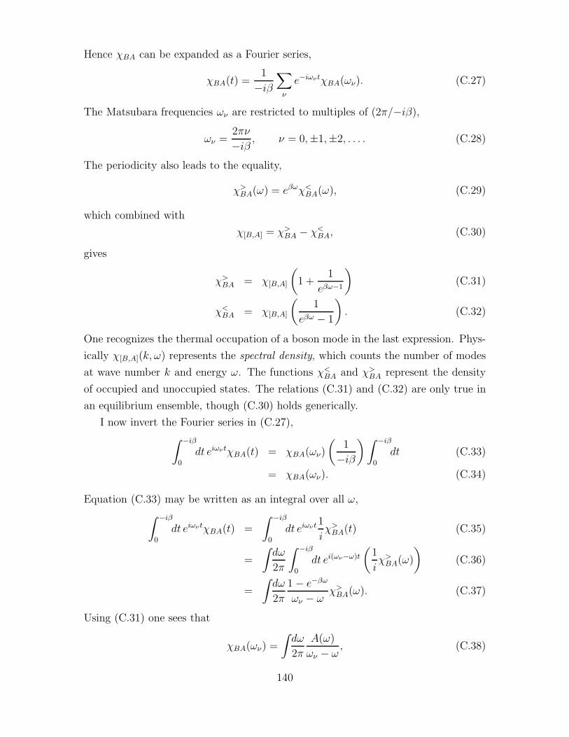
Hence χBA can be expanded as a Fourier series,
χBA(t) =1
−iβ∑
ν
e−iωνtχBA(ων). (C.27)
The Matsubara frequencies ων are restricted to multiples of (2π/−iβ),
ων =2πν
−iβ , ν = 0,±1,±2, . . . . (C.28)
The periodicity also leads to the equality,
χ>BA(ω) = eβωχ<
BA(ω), (C.29)
which combined with
χ[B,A] = χ>BA − χ<
BA, (C.30)
gives
χ>BA = χ[B,A]
(
1 +1
eβω−1
)
(C.31)
χ<BA = χ[B,A]
(
1
eβω − 1
)
. (C.32)
One recognizes the thermal occupation of a boson mode in the last expression. Phys-
ically χ[B,A](k, ω) represents the spectral density, which counts the number of modes
at wave number k and energy ω. The functions χ<BA and χ>
BA represent the density
of occupied and unoccupied states. The relations (C.31) and (C.32) are only true in
an equilibrium ensemble, though (C.30) holds generically.
I now invert the Fourier series in (C.27),
∫ −iβ
0
dt eiωνtχBA(t) = χBA(ων)
(
1
−iβ
)∫ −iβ
0
dt (C.33)
= χBA(ων). (C.34)
Equation (C.33) may be written as an integral over all ω,
∫ −iβ
0
dt eiωνtχBA(t) =
∫ −iβ
0
dt eiωνt 1
iχ>
BA(t) (C.35)
=
∫
dω
2π
∫ −iβ
0
dt ei(ων−ω)t
(
1
iχ>
BA(ω)
)
(C.36)
=
∫
dω
2π
1 − e−βω
ων − ωχ>
BA(ω). (C.37)
Using (C.31) one sees that
χBA(ων) =
∫
dω
2π
A(ω)
ων − ω, (C.38)
140

thus proving that the series coefficients χBA(ων) are equal to the Fourier transform
along the real axis χBA(ω = ων). Thus one can use the Matsubara Green’s functions
and the real-time Green functions interchangeably.
The real time Green’s functions because have obvious physical meaning, however
the imaginary time functions are easier to calculate. In the retarded real time func-
tions, temperature information is carried by the state of the system at time t = −∞.
In the time-ordered imaginary-time functions, temperature information is carried by
the cyclic boundary conditions. In both of these cases, it is only the unperturbed
system that is in thermodynamic equilibrium and the perturbation will in general
give a non-equilibrium state.
C.3 Sum rules
Often in working with this formalism that one has use for certain “sum rules.” These
involve taking various moments of χ[B,A](ω). The first rule is a statement that the
total spectral weight is given by the commutator of A and B,∫
dω
2πχ[B,A](ω) = χ[B,A](t = 0) = [B,A]. (C.39)
The second rule, known as the f-sum rule is
limω−>∞
ω2χBA(ω) =
∫
dω
2πωχ[B,A](ω) = i
∂
∂t
χ[B,A](t)
∣
∣
∣
∣
t=0
= [[B,H ], A]. (C.40)
The third rule is that∫
dω
2π
χ[B,A](ω)
ω= −χBA(ω = 0). (C.41)
The function χBA(ω = 0) is the static response of the system. It represents the
response of the system to very slowly turning on the perturbation. By definition, this
is the adiabatic, or isoentropic, response. One is also interested in the isothermal
response of the system, where the temperature of the system is held fixed while the
perturbation is turned on. Given specific quantities A and B one can use Maxwell
relationships to connect the two responses. In the general case it is simpler to use
the microscopics.
One defines the static isothermal response of B to a perturbation of the form
δH = αA, by writing
χ(T ) =δB
δα=
Tr e−βHB
Tr e−βH(C.42)
= −β [〈AB〉 − 〈A〉〈B〉] . (C.43)
141

By redefining A and B to be A = A− < A > and B = B− < B >, one can always
set 〈A〉〈B〉 = 0. Thus without loss of generality,
χ(T ) = −βχ<BA(t = 0) (C.44)
= −β∫
dω
2πχ<
BA(ω) (C.45)
= −β∫
dω
2πf(ω)χ[B,A](ω). (C.46)
Now if the spectral weight is concentrated at energies much less that T , then one can
replace f(ω) with (βω)−1, telling us χ(T ) ≈ χBA.
C.4 Green’s functions
This Appendix would not be complete without mentioning the most important re-
sponse function, the single particle Green’s function, which is the response of the
system to adding or removing a particle. As with more general response functions,
there is a whole zoo of Green’s functions, defined by
G(12) =1
i〈T(
Ψ(1)Ψ†(2))
〉 (C.47)
G<(12) = 〈Ψ(1)Ψ†(2)〉 (C.48)
G>(12) = 〈Ψ†(2)Ψ(1)〉 (C.49)
GR(12) =1
iθ(1 − 2)(G>(12) −G<(12)) (C.50)
GA(12) =−1
iθ(2 − 1)(G>(12) −G<(12)) (C.51)
A(12) = G>(12) −G<(12). (C.52)
Here a short hand notation is used where a number, such as 1, represents the time
and space coordinates t1 and r1. The Fourier transforms G<(ω) and G>(ω) are
particularly important as they give the density of available single-particle states and
the density of occupied single-particle states.
A convenient approach to calculating these Green’s functions is to approximate
and solve the partial differential equations that these functions obey. These equations
are derived from the equations of motion for the field operators. For concreteness,
considers a set of particles interacting through a point interaction of strength g, with
Hamiltonian
H =
∫
d3r∇Ψ†∇Ψ
2m− µΨ†Ψ +
g
2Ψ†Ψ†ΨΨ. (C.53)
142

Including the chemical potential µ in the Hamiltonian has no effect on the dynamics,
but makes thermodynamic relationships simpler. With this Hamiltonian, the field
operators obey an equation of motion
i∂tΨ(r, t) = [Ψ, H ] = −∇2r
2mΨ(r, t) − µΨ(r, t) + gΨ†(r, t)Ψ(r, t)Ψ(r, t). (C.54)
Multiplying on the right by Ψ†(r′, t′), time ordering and taking the expectation value,
(
i∂t +∇2
r
2m+ µ
)
G(rt, r′t′) − g〈TΨ†(r, t)Ψ(r, t)Ψ(r, t)Ψ†(r′, t′) = δ(t)δ3(r − r′).
(C.55)
The delta function on the right results from the time derivative of the time ordering
operator. Conventionally the interaction term is expressed in terms of a self-energy
Σ(rt, r′t′). The self-energy is most easily defined by expanding (C.55) in terms of the
Matsubara frequencies, and Fourier transforming with respect to r − r′;
(ων − k2/2m+ µ− Σ(k, ων))G(k, ων) = 1. (C.56)
The self-energy is typically calculated perturbatively. Some manipulations of these
equations are discussed in Chapter 6.
C.4.1 Anomalous Green’s functions
In the presence of a condensate the Green’s functions develop a matrix structure.
Here I briefly discuss the origin of this structure.
Since there are a macroscopic number of particles in a condensate, removing a
single particle from the condensed mode makes no difference to the system. This
property is captured by stating that the field operator Ψ has a non-zero expectation
value ψ = 〈Ψ〉. The function ψ(r) =√N0φ(r) corresponds to the square root of the
number of condensed particles times the wavefunction of the condensate. Thus the
field operator can be decomposed into a mean field part and fluctuations, Ψ = ψ+ ψ.
Taking the expectation value of (C.54),
(i∂t + ∇2/2m+ µ− g|ψ|2)ψ = 2gψ〈ψ†ψ〉 + gψ∗〈ψψ〉 + g〈ψ†ψψ〉. (C.57)
When the right hand side is neglected this equation is the Gross Pitaevskii equation,
which is accurate when the number of non-condensed particles is small. Many alkali
gas experiments are very well described by this “nonlinear Schrodinger equation.”
For a uniform condensate this equation is readily satisfied by setting µ equal to the
mean field energy, µ = gn0.
143
By considering the right hand side of (C.57) one sees that in addition to ordinary
Green’s functions of the form 〈ψ†ψ〉, one also has to consider anomalous Green’s
functions, 〈ψψ〉. The regular and anomalous functions are conveniently described by
a matrix
↔G(rt, r′t′) =
1
i
〈T(
ψ(r, t)ψ(r′, t′))
〉 〈T(
ψ(r, t)ψ(r′, t′))
〉〈T(
ψ(r, t)ψ(r′, t′))
〉 〈T(
ψ(r, t)ψ(r′, t′))
〉
. (C.58)
Analogous to (C.55), this matrix Green’s function obeys an equation of motion
(ωτ↔
3 − k2/2mτ↔
0 −Σ↔
(k, ω))↔G(k, ω) = τ
↔0. (C.59)
The matrix τ↔
3 is a Pauli matrix and τ↔
0 is the identity. A large class of approximations
for the self-energy are discussed in Appendix D. Where no confusion is likely to arise
I omit the ‘↔’ symbol on tensors and ‘→’ on vectors.
144
Appendix D
Conserving (Φ-derivable)
approximations
In this Appendix I review the structure of Φ-derivable Green’s function approxima-
tions, verifying that they obey the standard conservation laws (number, energy, and
momentum) [109]. These conservation laws are critical for correctly describing the
behavior of an atomic gas. A simple Φ-derivable approximation is used in Chapter
6.4. After a short discussion of conservation laws, I perturbatively develop Φ to sec-
ond order in the interactions. This second order functional in conjunction with the
kinetic theory of Chapter 6, provides a very accurate non-equilibrium theory of a
degenerate Bose gas.
D.1 Basic structure
As discussed in Section C.4.1, a condensed system is described by breaking up the
field operator Ψ into a mean field part ψ = 〈Ψ〉 and a fluctuation ψ. One is naturally
lead to a matrix formulation of the equation of motion where,
~ψ =
(
ψ
ψ†
)
(D.1)
↔G =
(
G11 G12
G21 G22
)
=1
i
(
〈ψψ†〉 〈ψψ〉〈ψ†ψ†〉 〈ψ†ψ〉
)
. (D.2)
The equations of motion for these functions are schematically written as
↔G−1
0~ψ = ~η (D.3)
(↔G−1
0 −Σ↔
)↔G = δ
↔. (D.4)
145

In these equations↔G−1
0 = iτ↔3∂t + ∇2/2mτ↔0, where τ↔3 is a Pauli matrix, τ↔0 is the
two-by-two identity matrix, and adjacent operators are convoluted. The symbol δ↔
=
δ(t − t′)δ3(r − r′)τ↔0 is the identity. The source term, ~η, and the self-energy, Σ↔
, are
complicated functionals of ~ψ and Σ↔
.
D.2 Conservation laws
One can guarantee conservation laws are satisfied if Σ↔
and ~η are related to a functional
of ψ and G via the relations [109],
2η =δΦ
δψ∗ (D.5)
iΣij =δΦ
δGji
, (D.6)
where ~η = (η, η∗). The symmetries of Φ give rise to conservation laws. For example,
conservation of particle number is related to the U(1) gauge symmetry of Φ. This
number conservation is easily demonstrated, starting with the identity
δΦ =
∫
d1∑
j
δΦ
δΨj(1)δΨj(1) +
∫
d1 d1′
[
∑
ij
δΦ
δGij(11′)δGij(11′)
]
(D.7)
=
∫
d1 2 (η∗(1)δψ(1) + η(1)δψ∗(1)) +
∫
d1 d1′∑
ij
iΣij(11′)δGji(1′1). (D.8)
Here a notational short-hand is used where the symbol 1 is used in place of time and
space co-ordinates t1, t1. I now consider a local gauge change of the form
~ψ → eiΛτ↔3 ~ψ (D.9)↔G → eiΛτ↔3
↔Ge−iΛτ↔3, (D.10)
which gives to lowest order
δψ = iΛψ (D.11)
δG = i(Λτ↔3
↔G−
↔Gτ↔3Λ). (D.12)
Thus the variation in Φ is
δΦ =
∫
d1 Λ(1) (2iη∗(1)ψ(1) − 2iη(1)ψ∗(1)) (D.13)
+
∫
d1 d1′ iΣ(11′) (iΛ(1′)τ3G(1′1) − iΛ(1)G(1′1)τ3)
=
∫
d1 Λ(1)
[
2i(η∗(1)ψ(1) − η(1)ψ∗(1)) (D.14)
−∫
d1′ Trτ3 (G(11′)Σ(1′1) − Σ(11′)G(1′1))
]
.
146

Since Φ is invariant under this gauge change, one must have δΦ = 0, for an arbitrary
choice of Λ, implying the expression in square brackets must vanish.
I now show that local number conservation is a consequence of this term vanishing.
From Eq. (D.1), ψ obeys the equation of motion(
i∂t +∇2
2m
)
ψ = η. (D.15)
Multiplying by ψ∗ and subtracting the complex conjugate yields
∂t(n0) + ∇ · (n0vs) = −i(ψ∗η − η∗ψ). (D.16)
Similarly, Eq. (D.2), reads(
iτ3∂t +∇2
2m
)
G(11′) = δ(11′) + Σ(12)G(21′). (D.17)
The adjoint equation to (D.17) reads
−i∂t′G(11′)τ3 +∇′2
2mG(11′) = δ(11′) +G(12)Σ(21′). (D.18)
Multiplying by τ3, subtracting the two equations, and setting 1′ = 1 yields
∂tiG(1, 1)+ ∇ ·[
1
2im(∇1τ3iG(1, 1′) −∇1′iG(1, 1′)τ3)
]
1=1′(D.19)
=
∫
d2 τ3Σ(12)G(21′) −G(12)Σ(21′)τ3.
Thus
∂t(2n) = ∂t(2n0 + TriG) (D.20)
= 2i(η∗ψ − ψ∗η) +
∫
d2 Tr τ3(Σ(12)G(21) −G(12)Σ(21)) (D.21)
which vanishes by virtue of Eq. (D.14).
D.2.1 Components
In some circumstances it is more convenient to work with the components Gij , rather
than the tensor↔G. The components are not independent. For example, G11(1, 1
′) =
G22(1′, 1). In computing the functional derivatives in (D.5), one needs to take the
interdependencies into account. To ensure that one does not double-count any terms,
it is convenient to take Φ, which is a functional of the matrix G(1, 1′), and substitute
G11(1, 1′) → G11(1, 1
′) +G22(1′, 1)
2(D.22)
G22(1′, 1) → G11(1, 1
′) +G22(1′, 1)
2. (D.23)
147

Call this new functional Φ′. The derivatives of Φ′ with respect to G12, G21, ψ, and
ψ†, are all trivially equal to the derivatives of Φ. To show that δΦ′/δG11 = δΦ/δG,
one writes
δΦ′
δG11(1′, 1)=
1
2
δΦ′
δG11(1′, 1)+
1
2
δΦ′
δG22(1, 1′)(D.24)
=Σ11(1, 1
′) + Σ22(1′, 1)
2(D.25)
= Σ11(1, 1′). (D.26)
In the rest of this Appendix, I make no distinction between Φ and Φ′. Equations
written in matrix notation will refer to Φ, while equations written in components will
refer to Φ′.
D.3 Self-energies
By definition, the self-energy is the sum of all irreducible diagrams which have one
incoming line and one outgoing line. (A diagram is irreducible if it cannot be split
into two by cutting a single propegator.) Figure D.1 shows all diagrams of Σ11 up to
second order in the interaction. All of the diagrams on each row are equal. Figure D.2
shows the diagrams for Σ12 to the same order. Algebraically, the diagonal elements
are−iΣ11(11′) = δ(1, 1′)2(−ig)(ψ∗ψ + iG11)
+2(−ig)2iG11(1′1)(iG11(11′)iG11(11′)−
i(G0)11(11′)i(G0)11(11′))
+4(−ig)2iG11(11′)iG12(11′)iG21(11′)
+4(−ig)2ψ(1)ψ∗(1′)iG12(11′)iG21(11′)
+2(−ig)2ψ∗(1)ψ(1′)(iG11(11′)iG11(11′)−i(G0)11(11′)i(G0)11(11′))
+4(−ig)2ψ(1)ψ(1′)iG11(11′)iG21(11′)
+4(−ig)2ψ∗(1)ψ∗(1′)iG11(11′)iG12(11′)
+4(−ig)2ψ(1)ψ∗(1′)iG11(11′)iG11(1′1)
+ · · · ,
(D.27)
148

Figure D.1: Terms in Σ11 up to second order in the interaction. Propegators, G11,
G12, and G21 are respectively represented by diagrams , , and . Inthe right hand columns the interaction is represented by a dashed line. For a pointinteraction, each of the diagrams on the right reduces to the diagram on the left inwhich the interaction is represented by a vertex with a dot. Short lines emanatingfrom vertices represent condensate contributions 〈ψ〉 and 〈ψ†〉.
149

(1) (1) (2) (4)
(2) (4) (4) (4)
(4)
Figure D.2: Terms in Σ12 which are up to second order in the interaction. Unlikefigure D.1, only the diagrams with point interactions are drawn, with the multiplicitylisted in parenthesis.
while the off-diagonal ones are
−iΣ12(11′) = δ(1, 1′)(−ig)(ψψ + iG12)
+2(−ig)2iG12(11′)iG12(11′)iG21(11′)
+4(−ig)2iG11(11′)iG11(1′1)iG21(11′)
+2(−ig)2ψ∗(1)ψ∗(1′)iG12(11′)iG12(11′)
+4(−ig)2ψ(1)ψ(1′)iG12(11′)iG21(11′)
+4(−ig)2ψ(1)ψ(1′)iG11(11′)iG11(1′1)
+4(−ig)2ψ∗(1)ψ(1′)iG11(11′)iG12(11′)
+4(−ig)2ψ(1)ψ∗(1′)iG11(1′1)iG12(11′)
+ · · · .
(D.28)
Here Σ is self-consistent; the expressions above use G and not G0. The interaction
g = 4π~2as/m is not the bare interaction, but rather comes from a repeated summing
of binary interactions (the T-matrix), and to avoid double counting one must subtract
the G0’s which appear in the above equations.
150
The source term in the condensate’s equation of motion η is given by
η = g〈Ψ†ΨΨ〉= gψ∗ψψ + 2gψiG11 + gψ∗iG12
−ig2
2
∫
d3r
∫ −iβ
0
dτ [4ψ∗(1′)iG21(11′)iG11(11′)iG11(11′)
+4ψ(1′)iG11(1′1)( iG11(11′)iG11(11′)−
i(G0)11(11′)i(G0)11(11′))
+8ψ∗(1′)iG11(11′)iG11(1′1)iG12(11′)
+8ψ(1′)iG11(1′1)iG12(11′)iG21(11′)]
+ · · · .
(D.29)
These expressions are summed up by writing down Φ. To ease notation, we will
use G→ as a short form of (G11 +G22)/2.
Φ = g
∫
d1
[
|ψ|4 + 4|ψ|2iG→ + (ψ∗)2iG12 + (ψ)2iG21 + 2iG→iG→
]
−ig2
3
∫
d1 d1′[
3iG→(11′)iG→(11′)iG→(1′1)iG→(1′1)
+3iG12(11′)iG21(11′)iG12(1′1)iG21(1
′1)
+12iG→(11′)iG12(11′)iG→(1′1)iG21(1′1)
+12ψ(1)ψ∗(1′)iG→(11′)iG→(1′1)iG→(1′1)
+6ψ(1)ψ(1′)iG12(11′)iG12(1′1)iG21(1
′1)
+6ψ∗(1)ψ∗(1′)iG21(11′)iG21(1′1)iG12(1
′1)
+12ψ∗(1)ψ∗(1′)iG→(11′)iG21(1′1)iG→(1′1)
+12ψ(1)ψ(1′)iG→(11′)iG12(1′1)iG→(1′1)
+ 24ψ(1)ψ∗(1′)iG→(11′)iG12(1′1)iG21(1
′1)
]
.
(D.30)
Φ differs from the free energy in that the second order terms have an extra factor of
1/3. The relevant diagrams are shown in Fig. D.3.
151

(2) (1)
(4) (1) (1)
(3) (3) (12)
(12) (6) (6)
(12) (12) (24)
Figure D.3: Second order expansion of Φ in powers of V . Only the diagrams withpoint interactions are drawn, but the multiplicity is listed in parenthesis.
152

Appendix E
Collisionless Excitations of a
Spatially Uniform Weakly
Interacting Gas
E.1 Introduction
In this Appendix I calculate the linear response of a gas of degenerate atoms in the
collisionless regime. These results were used in Chapter 5 to calculate the stability
of a gas of attractive atoms, and are the building blocks for the more sophisticated
kinetic theory described in Chapter 6.
I begin by discussing a simple classical kinetic theory, the collisionless Boltzmann
equation. I linearize this equation about equilibrium to find the elementary excita-
tions of a classical gas. I show that a classical gas has a collisionless “zero-sound”
mode that has the same dispersion relationship as the Bogoliubov spectrum of a
zero temperature Bose gas. I then go through the equivalent procedure in a quan-
tum mechanical system, producing the random phase approximation, and finding the
excitation spectrum of a uniform Bose gas at arbitrary temperature. Those unfa-
miliar with the general theory of linear response functions may wish to glance at
Appendix C, where I give a brief review of the subject.
E.2 The collisionless Boltzmann equation
I begin with a discussion of the collisionless Boltzmann equation, which describes
a classical gas of particles with a mean-field treatment of their interactions. This
equation is used in plasma physics, where its known as the Vlasov equation. Treating
153

the interactions via a mean-field, and introducing a weak perturbing field U(x, t), the
particles see a potential
V (x, t) = gn(x, t) + U(x, t), (E.1)
where g parameterizes the interaction. In the absence of U , the density n is uniform.
Denoting the distribution of particles with momentum p, and position x, at time
t, by f(p, x, t), the collisionless Boltzmann equation reads
∂tf(p, x, t) + v · ∇xf(p, x, t) + F · ∇pf(p, x, t) = 0. (E.2)
This equation simply states Newton’s laws. The particles drift with velocity v = p/m,
and accelerate according to the force F = −∇xV (x, t). Note that the density in (E.1)
is
n(x, t) =
∫
dp
(2π)3f(p, x, t). (E.3)
In the absence of the perturbation U(x, t), the Boltzmann equation is solved by
the Maxwellian velocity distribution
f0(p, x, t) = e−β(p2/2m+gn−µ). (E.4)
The density n is uniform and solves the equation n = eβµ−gn/Λ3, where Λ−2 =
mkBT/2π~2 is the thermal wavelength. Linearizing (E.2) about this solution gives
∂tδf + v · ∇xδf + βf0v · ∇x(U + gδn) = 0, (E.5)
where δf and δn are respectively the variation of f and n.
It is convenient to Fourier transform (E.5) with respect to space and time, using
the convention
g(k, w) =
∫
dx
∫
dt e−ik·x+iωtg(r, t). (E.6)
Note, there are two momenta in the resulting equations; p = mv is the physical
momentum of the particles, and ~k is the momentum associated with the Fourier
transform of x. The transformed equation reads
−ωδf + v · kδf + βf0v · k(U + gδn) = 0. (E.7)
If g = 0, then δf = βf0(v · k/(v · k − ω)). Integrating over p, the response of the
noninteracting gas is
χ0 =δn
δU
∣
∣
∣
∣
g=0
=
∫
dp
2π3
βf0 v · kω − v · k . (E.8)
154

In the complex frequency plane, this function contains a branch cut along the real
frequency axis. In most circumstances one is interested in the retarded response,
which is the analytic continuation from the upper half plane. One selects out this
branch by taking ω → ω + iη in (E.8). Equation (E.7) is no more difficult to solve
when g 6= 0. Solving for δf and integrating over p gives
δn = χ0(U + gδn). (E.9)
This equation is interpreted as saying that the cloud responds not only to the external
potential, but also to the mean field generated when its profile is distorted. The full
response function is written as
χ =δn
δU=
χ0
1 − gχ0. (E.10)
This expression involves all powers of the interaction.
To understand the response (E.10) one first needs to understand the structure of
χ0. In Eq. (E.8), the integral over the directions transverse to k is trivial, leaving
χ0(k, ω) = −βn 1√π
∫
dtt e−t2
t− ω/νk. (E.11)
All the k-dependence in this expression is buried in the characteristic energy scale
νk = 2√
ǫkT . (E.12)
For ease of reference, I denote the integral as
I(x) =1√π
∫
dtt e−t2
t− x. (E.13)
I(x) can be written in terms of standard functions by expanding the ratio t/(t−x)as a Fourier integral,
I(x) = 1 +2ix√π
∫ ∞
0
ds
∫
dte−t2−2ist+2ixs. (E.14)
The t integral is Gaussian, as is the subsequent s integral. In terms of the error
function erf(z) = (2/√π)∫ z
0exp(−z2), the integral is
I(x) = 1 + i√πxe−x2
(1 − erf(−ix)). (E.15)
The singularities of I(x) all reside at x = −i∞, signifying that any collective modes
of the system are strongly overdamped. As I now show, in the interacting gas, these
155

singularities move towards the real axis, and for sufficiently strong interactions a
collective “zero-sound” mode develops.
A useful trick for understanding the poles of the interacting system is to find the
curves in the complex plane where Im(χ0) = 0, as shown in Fig. E.1. The poles of χ
lie along these lines. The zeroes of χ0 appear as the intersection of two of these lines.
In the context of attractive interactions, the most important line of Im(χ0) = 0 lies
on the imaginary axis, where as ω → −i∞ the function I(ω) diverges to +∞, but as
ω → i∞, the function I(ω) → 0. For attractive interactions g < 0, the pole on this
line starts at ω = −i∞, but as interactions increase, the pole moves upwards. When
βgn = −1, the pole reaches the real axis. For larger interactions, the pole crosses onto
the physical sheet – signaling a breakdown of our approach. As described by Mermin
[132], the pole crossing the real axis represents the spinodal line of a liquid-gas phase
transition.
There is no instability for repulsive interactions. Instead there is a collective mode,
whose frequency is given by the location of the pole on the line Im(χ0) = 0 which
asymptotically approaches the real axis. One finds the dispersion of this excitation
by looking at the large x expansion, I(x) = −1/2x2 + O(x−4). Using (E.10), the
formula for χ, one arrives at
χ =2nǫk
ω2 − 2ngǫk. (E.16)
Thus there is a mode with linear dispersion ω = ck, where the speed of sound is
c =√
ng/m. For consistency of the large x expansion, one must have ω2 ≫ ν2k = ǫkT ,
which translates into ng ≫ T . In other words, this mode exists as long as the mean-
field interactions dominate the temperature. It is no coincidence that this mode has
the same dispersion as the zero-temperature Bogoliubov sound mode.
E.3 Random phase approximation
In this Section I perform the same calculation in the quantum regime. Much of the
hard work has already been done in 1974 by Szepfalusy and Kondor [107], who were
interested in how the modes below Tc match up with the modes above Tc. This
investigation lead them to calculate the response of an interacting gas within the
random phase approximation (RPA). They considered only the repulsive case, but it
is not difficult to extend their work into the the more general setting.
The starting point, as before, is to calculate the density response function χ =
156

0 1 2 3 4Re@ΩΝkD
-4
-3
-2
-1
0
Im@ΩΝkD
Figure E.1: Zeros of the imaginary part of the free response function χ0(k, ω) as afunction of complex ω. The sign of χ0 alternates on adjacent contours. In particular,the line on the imaginary axis has χ0 < 0, and the one to its right has χ0 > 0.Within a mean-field approximation, these lines represent the paths which the poles ofχ follow as one increases the strength of the interactions. For attractive interactions,the singularities follow the χ0 < 0 lines, while for repulsive interactions, they followthe χ0 > 0 lines. In all cases the poles reside at ω = −i∞ when the interactionsvanish. In the case of attractive interactions, a pole can cross the x axis, representing amechanical instability. In the case of repulsive interactions, a pole can asymptoticallyapproach the real axis, representing a collective “zero sound” mode.
157

δn/δU . The simplest approximation, the RPA, consists of a sum over bubbles,
χ =χ0
1 − gχ0
. (E.17)
The physics here is the same as in the classical case. The density response is the direct
response, plus the response to the mean field generated by the distorted density profile.
The approximation comes in treating the direct response as χ0, the susceptibility of
the non-interacting system.
The most elementary approach to calculating χ0 is to simply write down the
response function in the time domain (cf. Appendix C)
χ0 =δρq(0)
δUq(t)=
1
i
[
〈T(
ρ†q(t)ρq(0))
〉0 − 〈ρ†q(t)〉0〈ρq(0)〉0]
, (E.18)
where ρq is the Fourier transform of the density operator,
ρq =
∫
d3r eiq·r 〈ψ†(r)ψ(r)〉 =∑
k
a†k+q/2ak−q/2. (E.19)
The real-space operator ψ(r) annihilates a particle at position r, while the momentum
space operator ak annihilates a particle with momentum k. Although I write n for the
mean density, I use ρk, rather than nk for the Fourier component of the density. The
symbol nk denotes the number of particles in a mode with momentum k; nk = a†kak.
For the non-interacting system, the product of the two density operators in (E.18)
factors, leaving a simple bubble,
χ0 =1
i
∑
k
〈T(
a†k−q/2(t)ak−q/2(0))
〉0〈T(
ak+q/2(t)a†k+q/2(0)
)
〉0. (E.20)
Since the field operators evolve as
ak(t) = e−iǫktak(0), (E.21)
one can trivially perform the Fourier transform to arrive at
χ0(q, ω) =∑
k
nk−q/2 − nk+q/2
ω − (ǫk+q/2 − ǫk−q/2). (E.22)
A more sophisticated yet computationally simpler (and more instructive) way to
arrive at the same formula is to write (cf. Eq. (C.12)
〈T(
ρ†qρq
)
〉(ω) =
∫
dω′
2π
Π(q, ω′)
ω − ω′ , (E.23)
where
Π(q, ω) = −2Imχ0 = 〈[ρ†q, ρq]〉(ω). (E.24)
158

As the imaginary part of χ, Π represents a decay rate – the rate at which particles
scatter from momentum k − q/2 to momentum k + q/2.
Looking at the two terms in the commutator, one sees that there are two processes
in Π. In the first process, a particle comes along with momentum k−q/2 and scatters
into a state with momentum k+q/2, gaining an energy ω. The second process (which
has a minus sign) has a particle with momentum k+ q/2 scattering into a state with
momentum k − q/2, losing energy ω. Thus the spectral density is
Π(q, ω) =∑
k
[(
nk−q/2(1 + nk+q/2) − nk+q/2(1 + nk−q/2))
(2πδ(ǫk+q/2 − ǫk−q/2 − ω)]
,
(E.25)
which when substituted into (E.23) gives the same result as (E.22).
I now replace the sum over k with an integral. This is allowed as long as I treat the
condensate separately (cf. the discussion in Chapter 2). Thus, following Szepfalusy
and Kondor, I break the response function up into a regular part due to the non-
condensed particles, and a singular part due to the condensate, χ0 = χn0 + χc
0. The
regular part is
χn0 (q, ω) =
∫
d3k
(2π)3
nk−q/2 − nk+q/2
ω − (ǫk+q/2 − ǫk−q/2), (E.26)
and the singular part is
χc0(q, ω) =
n0
ω − ǫq− n0
ω + ǫq. (E.27)
At zero temperature, only the singular part contributes, χ0 = χc0. Thus the response
function of the interacting system is
χ =χ0
1 − gχ0
=2n0ǫq
ω2 − ǫ2q − 2n0gǫq. (E.28)
Clearly, one has well defined excitations with energies given by the Bogoliubov ex-
pression
ω =√
ǫ2q + 2gn0ǫq. (E.29)
As discussed in Section 5.2.2, for attractive interactions one finds an instability when
the level spacing ~2/2mL2 is equal to −2gn0. In the opposite limit of T ≫ Tc, only the
regular part contributes, χ0 = χn0 , and the distribution functions nq become classical
nq = e−β(ǫq−µ). Linearizing both the numerator and denominator of (E.26) in q allows
us to recover the result of Section E.2,
(χ0)classical = −βnI(ω/νq). (E.30)
159

To discuss the intermediate regime (between zero T and classical) one has to study
the analytic structure of χn0 . First, however, I introduce a more sophisticated version
of the RPA, first used by Minguzzi and Tosi [108]. This improved approximation
includes exchange forces, which are important for short range interactions.
E.3.1 The RPA with exchange
Equation (E.17) was based upon the assumption that the response to a perturbation
δU is given by the classical result δn = χ0(δU + gδn). This expression ignores
exchange processes where the identical particles exchange momenta. By including
this exchange term one produces Hartree-Fock approximation, δn = χ0(δU + 2gδn).
Unfortunately, this last expression cannot be applied to a condensed gas. The problem
is that this factor of two only occurs if the coliding particles are in different states.
Thus a scheme must be devised to account for the exchange interaction between
non-condensed particles, but not between condensed ones.
Such a scheme was developed by Minguzzi and Tosi [108]. One looks separately at
the change in the density of condensed and non-condensed atoms, δn0 and δn. The
factors of two are easily incorporated in a matrix expression,(
δn0
δn
)
=
(
χc0
χn0
)
δU +
(
χc0 2χc
0
2χn0 2χn
0
)(
gδn0
gδn
)
, (E.31)
which gives the relationship
χ =δn0
δU+δn
δU=
χc0 + χn
0 + gχc0χ
n0
(1 − gχc0)(1 − 2gχn
0) − 4g2χc0χ
n0
. (E.32)
An alternative view of this same approximation is to use Eq. E.17, but include the
exchange interaction in χ0. For example, for a non-condensed gas in the Hartree-Fock
approximation, one would write
χHF0 = χn
0
(
1 + gχn0n+ (gχn
0n)2 + · · ·)
, (E.33)
where successive exchange collisions are accounted for. Diagrammatic expressions for
these different approximations are shown in Fig. E.2.
E.4 Analytic Structure of χn0
In this Section I investigate the analytic structure of χn0 . Section E.4.1 will be devoted
to deriving the following expression [107]
χn0 (k, ω) = − m
πkΛ2T
∫ (ω+ǫk)/νk
(ω−ǫk)/νk
dz
∫
dxx
x− z
1
ex2−βµ − 1, (E.34)
160

χ = + + + ...a)
b)
c)
d)
e)
H=
HF= + + + ...
H= + +
HF= + + + +
+ +
++ ++
+
+ +
+ ++
+ ...
Figure E.2: Diagrammatic description of the approximation used for the responsefunction. Lines with arrows represent propegators of the non-interacting system.Jagged lines represent the contact interaction between particles. a) Generically theresponse function can be expressed in terms of a polarization bubble (the bubble withshaded interior). b) In the Hartree approximation (RPA), the polarization bubble istaken to be the response of the non-interacting gas. c) In the Hartree-Fock approxi-mation, the polarization bubble involves a sum over repeated exchange interactions.d) In a condensed system, the polarization bubble for the Hartree approximation mustinclude terms where one of the particles is in the condensate. e) The Hartree-Fockapproximation for the condensed gas requires writing all exchange graphs, noting thatthere is no exchange interaction between condensed atoms. The vertices in these fig-ures with only a single solid line implicitly include an interaction with the condensate.
161
where once again νk = 2√Tǫk. Following this derivation I will give the asymptotic
behavior of χn0 in various limits.
The x integral in (E.34) is the quantum mechanical version of the integral I(t)
introduced in Section E.2, and it shares many of the same analytic structures (for
example it is a meromorphic function). The response function χ, is not meromorphic,
as it contains logarithmic singularities in the complex frequency plane.
E.4.1 SK expression
In this section I derive Eq. (E.34). Starting with the general expression,
χn0 (k, ω) =
∫
d3q
(2π)3
nq−k/2 − nq+k/2
ω − (ǫq+k/2 − ǫq−k/2), (E.35)
one splits the integrand into two terms, one containing nq−k/2 and the other nq+k/2.
After shifting q by ±k/2, one finds
χn0 (k, ω) =
∫
d3q
(2π)3nq
(
1
ω − (ǫq+k − ǫq)− 1
ω − (ǫq − ǫq−k)
)
. (E.36)
The energies in the denominator can be expanded as ǫq±k = (q2 +k2 ±2kq cos θ)/2m,
where cos θ is the angle between q and k. The angular integrals are easily performed,
leading to
χn0 (k, ω) =
m
(2π)2k
∫ ∞
0
dq q2 nq log
[
(p+ k/2 − q)(p− k/2 + q)
(p+ k/2 + q)(p− k/2 − q)
]
, (E.37)
with p = mω/k. One extracts the important structure by rewriting the logarithm
as an integral of the form∫
dx/x. Scaling all lengths by a multiple of the thermal
wavelength gives
χn0 (k, ω) =
−mπkΛ2
T
∫ z+
z−
dz I(z, βµ) (E.38)
I(z, βµ) =
∫ ∞
−∞dx
x
x− z
1
ex2−βµ − 1, (E.39)
where z± = ω/2√εkT ± kΛT/4
√π. In the limit βµ → ∞, I(z, βµ) agrees with the
function I(z) defined on p. 155.
E.4.2 ω → ∞ structure of χn0 .
Here I investigate the high frequency response of the noninteracting system. This is
a useful check on our analysis as the exact structure is a consequence of the f-sum
162

rule. As ω → ∞, the limits z± in the integral in (E.38) become very large, and one
can expand (E.39) in powers of 1/z,
I(z, βµ) → − 1
z2
∫
dx x2 1
ex2−βµ − 1(E.40)
= − 1
z2
∑
j
eβjµ
∫
dxx2e−jx2
(E.41)
= −Γ(3/2)
z2
∑
j
eβjµ
j3/2(E.42)
= −√π
2
g3/2(eβµ)
z2. (E.43)
Thus if ω ≫ ǫk the response function is
χn0 (k, ω) = − m
πkΛ2T
∫ (ω+ǫk)/νk
(ω−ǫk)/νk
dz
∫
dxx
x− z
1
ex2−βµ − 1(E.44)
→ − m
πkΛ2T
(
2ǫkνk
)
I[ω/νk, βµ] (E.45)
=2ǫkn
ω2, (E.46)
where I’ve used that n = g3/2(eβµ)/Λ3
T . This is the result expected from the f-sum
rule.
E.4.3 Long wavelength response
According to Eq. (E.38), at fixed ω, the k → 0 limit of χn0 is equivalent to the ω → ∞
limit. Further analysis is needed to understand the k → 0 structure as ω → 0.
Analytic structure of I.
The first step to understanding the low frequency, long wavelength response is to write
I in terms of its poles in the complex z plane. This is accomplished by expanding
the distribution function in terms of Matsubara frequencies,
1
ex2−βµ − 1=∑
ν
1
x2 − βµ− 2πiν, (E.47)
so that
I(z, βµ) =
∫
dx1
ex2−βµ − 1+ z2
∫
dx1
x2 − z2
(
∑
ν
1
x2 − βµ− 2πiν
)
.(E.48)
163

The first integral is a Bose function√πg1/2(e
βµ). The second integral is evaluated
with the residue theorem,
I(z, βµ) =√πg1/2(e
βµ) − iπz
2+ iπ
∑
ν
(
1
z −√βµ+ 2πiν
+1√
βµ+ 2πiν
)
. (E.49)
The branches of the square roots are chosen so that they poses negative imaginary
parts. This agrees with formula (A.3) of Szepfalusy and Kondor, even though their
expression is much more complicated looking. At degeneracy, βµ → 0, and (E.49)
becomes
I = π1/2ζ(1/2)− iπz
2+iπ
z+ iπ
∑
ν 6=0
(
1
z −√
2πiν+
1√2πiν
)
. (E.50)
The k → 0 limit of χ(ω = 0)
Integration of the leading terms and setting ω = 0 yields Eq. (5.8),
gχn0(k, 0) = −2
as
ΛT
[
4π
kΛT
arctan |εk/4µ|1/2 + g1/2(eβµ) − |π/βµ|1/2 + O(kΛT )
]
.
(E.51)
The expansion parameter is z+ = kΛT/4√π.
Asymptotics of the T-matrix
This is an appropriate place to discuss the asymptotics of the function Ξ, defined by
(5.16). This function is analogous to χn0 , except it corresponds to a response in the
particle-particle channel. Following the procedure of sec. E.4.1 to integrate out the
angular variables, one writes Ξ as
Ξ(k, ω) =−2m
πkΛ2T
∫ z+
z−
dz I(z), (E.52)
with z± = (kΛ/4√π)[i√
1 + 2ω/εk ± 1]. Using the expansion in Eq. (E.49) gives Eq.
(5.17),
gΞ(k, ω = 0) = −4as
ΛT
[
4π
kΛTarctan
(
|ǫk/4µ|1/2
1 + |ǫk/4µ|1/2
)
(E.53)
+g1/2(eβµ) − |π/βµ|1/2 + O(kΛT )
]
.
164

E.4.4 The classical limit revisited
I now re-examine the classical limit discussed in Section E.2. My procedure there
amounted to using a linearized dispersion, effectively confining the result to ω ≫ ǫk.
It is possible to calculate the exact result, in order to separate the quantum effects
in (E.34) from the non-linear effects. I start with
χn0 (k, ω) = − m
πkΛ2T
∫ (ω+ǫk)/νk
(ω−ǫk)/νk
dz
∫
dxx
x− z
1
ex2−βµ − 1, (E.54)
then take the classical limit 1/(ex2−βµ−1) → e−(x2−βµ), and use the identity m/2πk =
1/ΛTνk
√π, in order to get
χn0 (k, ω)c = −βn νk
2ǫk
1√π
∫ (ω+ǫk)/νk
(ω−ǫk)/νk
dz
∫
dxxe−x2
x− z, (E.55)
where, as usual, n = eβµ/Λ3T . Turning back to Section E.4.1, one sees that the last
integral is
χn0 (k, ω)c = −βn νk
2ǫk
∫ (ω+ǫk)/νk
(ω−ǫk)/νk
dz[
1 + i√πxe−x2
(1 − erf(−ix))]
. (E.56)
Integrating by parts leaves us with the final expression
χn0 (k, ω)c = βn
νk
2ǫk
i√π
2
[
e−t2(1 + erf(it))]t=(ω+ǫk)/νk
t=(ω−ǫk)/νk
. (E.57)
Note that even when ω = 0, this expression epends on ǫk,
χn0 (k, ω = 0)c = −βn
√πe−(ǫk/νk)2erf(iǫk/νk)
2(ǫk/νk). (E.58)
For ǫk ≪ T one can expand (E.58) in powers of ǫk/νk,
χn0 (k, ω = 0)c = −βn
(
1 − 2
3
(
ǫkνk
)2
+4
15
(
ǫkνk
)4
+O(ǫk)
)
. (E.59)
165

Appendix F
Low Energy Scattering
In this Appendix I review the theory of low energy scattering. This subject is par-
ticularly important for understanding Feshbach resonances, where the interactions
between atoms are tuned by changing the magnetic field.
F.1 The Scattering amplitude
F.1.1 Definition
The basic picture of potential scattering is illustrated in Fig. F.1. One has an incoming
wave eikz that is incident on a small impurity of size r0 (positioned at the origin), and
one asks what the far field wavefunction looks like. Generically
ψ(r) = eikz + f(k, r)eikr
r, (F.1)
which has the form of the incoming wave plus a scattered wave. In the far field r ≫ r0,
the scattering amplitude f can only be a function of the incident wave vector k, and
on the direction r. (In this equation f is also implicitly a function of the direction
of the incoming wave, generically denoted k and here set to z. For a spherically
symmetric potential f is independent of k.)
In the long wavelength limit kr0 ≪ 1 one expects that the scattering will become
isotropic – the wave is too large to “see” the structure of the impurity. Thus one can
drop the r dependences and only consider f(k), referred to as the s-wave scattering
amplitude. All of our discussions will be limited to this s-wave limit. The same
argument implies that f does not have much momentum dependence. For the most
part this statement is true and f can be replaced by f(k = 0); however in the presence
of a scattering resonance, f depends strongly on k. These resonances are of immense
experimental importance.
166
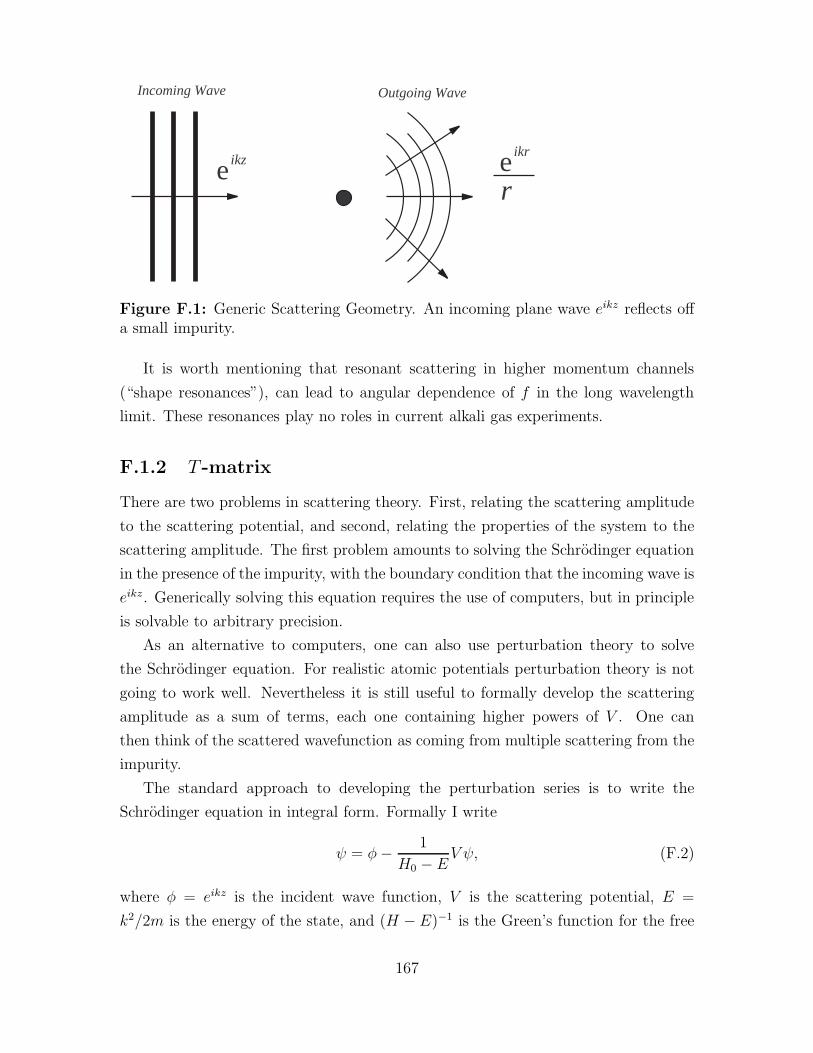
eikz
Incoming Wave Outgoing Wave
eikr
r
Figure F.1: Generic Scattering Geometry. An incoming plane wave eikz reflects offa small impurity.
It is worth mentioning that resonant scattering in higher momentum channels
(“shape resonances”), can lead to angular dependence of f in the long wavelength
limit. These resonances play no roles in current alkali gas experiments.
F.1.2 T -matrix
There are two problems in scattering theory. First, relating the scattering amplitude
to the scattering potential, and second, relating the properties of the system to the
scattering amplitude. The first problem amounts to solving the Schrodinger equation
in the presence of the impurity, with the boundary condition that the incoming wave is
eikz. Generically solving this equation requires the use of computers, but in principle
is solvable to arbitrary precision.
As an alternative to computers, one can also use perturbation theory to solve
the Schrodinger equation. For realistic atomic potentials perturbation theory is not
going to work well. Nevertheless it is still useful to formally develop the scattering
amplitude as a sum of terms, each one containing higher powers of V . One can
then think of the scattered wavefunction as coming from multiple scattering from the
impurity.
The standard approach to developing the perturbation series is to write the
Schrodinger equation in integral form. Formally I write
ψ = φ− 1
H0 − EV ψ, (F.2)
where φ = eikz is the incident wave function, V is the scattering potential, E =
k2/2m is the energy of the state, and (H − E)−1 is the Green’s function for the free
167

Schrodinger equation. Applying H0 − E to Eq. (F.2), one arrives at
(H0 − E)ψ = −V ψ, (F.3)
which is the conventional Schrodinger equation.
As can be verified directly, in momentum space and in real space, the Green’s
functions are given by
〈q| 1
H −E|q′〉 =
(2π)3δ3(q − q′)
q2/2m− E(F.4)
〈r| 1
H −E|r′〉 =
m
2π
exp(ik|r − r′|)|r − r′| , (F.5)
where E = k2/2m. On physical grounds, I have chosen outgoing boundary conditions
in Eq. (F.5). This latter result is only true in three dimensions. Getting away from
my schematic notation, one writes Eq. (F.2) in one of two forms,
ψ(k′) = (2π)3δ3(kz − k′) − 2m
∫
d3q
(2π)2
V (k′ − q)
q2 − (k′)2ψ(q), (F.6)
ψ(r) = eikz − m
2π
∫
d3r′eik|r−r′|
|r − r′|V (r′)ψ(r′), (F.7)
The first equation is in momentum space, the second in real space. In this Section
I only consider the real space equation (F.7), though later I will focus on (F.6). For
simplicity I assume that V (r) falls off over a lengthscale r0. Longer range potentials
can be treated, but such analysis is not particularly important for discussing neutral
atoms.
In the far field, r ≫ r0, one can expand the difference |r− r′| in the integral, to
arrive at the equation
ψ(r) = eikz − m
2π
eikr
r
∫
d3r′ eikr·r′V (r′)ψ(r′). (F.8)
Comparison with Eq. (F.1) gives an expression for the scattering amplitude,
f(k, r) = −m
2π
∫
d3r′ eikr·r′V (r′)ψ(r′). (F.9)
One generates a perturbative solution to Eq. (F.7) by a simple iterative scheme.
One starts by setting ψ(r) = eikz on the right hand side of (F.7). This first order
result is known as the Born approximation to scattering. This procedure is iterated
by substituting the new value of ψ into the right hand side. In a schematic notation,
one has
ψ =
(
1 − 1
H0 − EV +
1
H0 − EV
1
H0 −EV +
1
H0 − EV
1
H0 − EV
1
H0 −EV + · · ·
)
φ.
(F.10)
168

= + + ...+
= +
Figure F.2: Diagrammatic representation of the T-matrix equation. The T-matrix,designated by a dark dashed line connected to an “X”, comes from multiple scatteringoff the potential. The soft dashed lines represent bare potential scattering.
This expression is compactly written as
ψ = ψ0 −1
H0 − ETψ0, (F.11)
where the T-matrix is defined by
T = V + V1
H0 −EV + V
1
H0 − EV
1
H0 − EV + · · · (F.12)
= V + V1
H0 −ET. (F.13)
A diagrammatic representation of Eq. (F.12) is shown in Fig. F.2. The scattering
amplitude is then related to the on-shell T-matrix, by the expression
f(k) =−m2π~2
T (k). (F.14)
For the many-body problem, or for the problem of scattering off many impurities,
one in principle needs the off shell T-matrix.
To fully appreciate the structure of the T-matrix, one must go beyond s-wave
scattering, and consider the generic scattering amplitude f(k, r, k) defined by the
asymptotic form
ψ(r) = eik·r + f(k, k, r)eikr
r. (F.15)
The scattering amplitude is a function of the direction of the incoming wave k, the
direction of the outgoing wave r, and the energy of the scattering particle, k2/2m.
The T -matrix similarly is a function of three variables,
T (k,k′, q) ≡ 〈k′|T (E = q2/2m)|k〉 (F.16)
= 〈k′|V |k〉 + 〈k′|V 1
H0 −ET |k〉. (F.17)
The variables are the incoming momentum k, the outgoing momentum k′, and the
energy E = q2/2m. If one sets |k| = |k′| = q, one finds
f(k, k, r) = −m
2πT (kk, kr, k). (F.18)
169
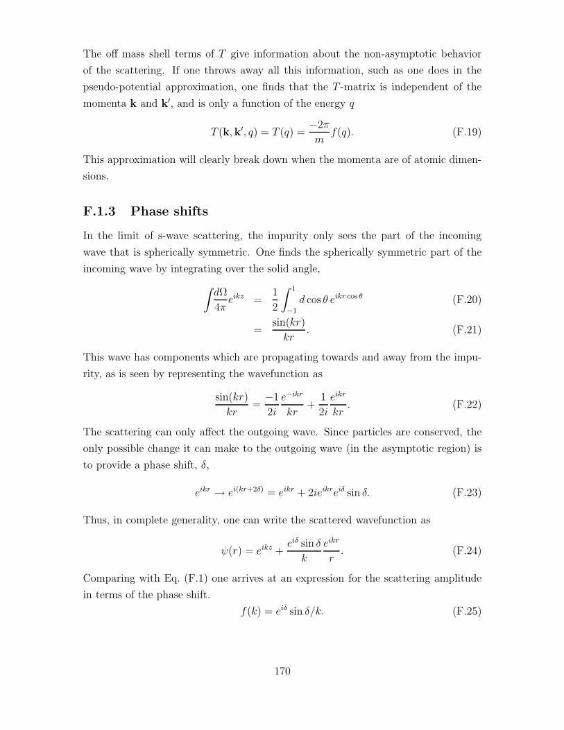
The off mass shell terms of T give information about the non-asymptotic behavior
of the scattering. If one throws away all this information, such as one does in the
pseudo-potential approximation, one finds that the T -matrix is independent of the
momenta k and k′, and is only a function of the energy q
T (k,k′, q) = T (q) =−2π
mf(q). (F.19)
This approximation will clearly break down when the momenta are of atomic dimen-
sions.
F.1.3 Phase shifts
In the limit of s-wave scattering, the impurity only sees the part of the incoming
wave that is spherically symmetric. One finds the spherically symmetric part of the
incoming wave by integrating over the solid angle,
∫
dΩ
4πeikz =
1
2
∫ 1
−1
d cos θ eikr cos θ (F.20)
=sin(kr)
kr. (F.21)
This wave has components which are propagating towards and away from the impu-
rity, as is seen by representing the wavefunction as
sin(kr)
kr=
−1
2i
e−ikr
kr+
1
2i
eikr
kr. (F.22)
The scattering can only affect the outgoing wave. Since particles are conserved, the
only possible change it can make to the outgoing wave (in the asymptotic region) is
to provide a phase shift, δ,
eikr → ei(kr+2δ) = eikr + 2ieikreiδ sin δ. (F.23)
Thus, in complete generality, one can write the scattered wavefunction as
ψ(r) = eikz +eiδ sin δ
k
eikr
r. (F.24)
Comparing with Eq. (F.1) one arrives at an expression for the scattering amplitude
in terms of the phase shift.
f(k) = eiδ sin δ/k. (F.25)
170

F.1.4 Meaning of the scattering amplitude and the phase
shift
On a microscopic level, δ has a clear meaning. It is the phase shift of the scattered
wave, relative to what it would be without the impurity. In the following section I
will show how this phase shift can be simply related to the density of states in the
presence of the impurity. The scattering amplitude, f , is the amplitude that the
particles are scattered. That is, σ = 4π|f |2 is the number of scattered particles per
unit flux of incoming particles. The cross section σ is the area that a classical target
would have to have for the scattering probability to be the same.
An equivalent way to understand f is to look at the equation
ψ = eikz + feikr
r. (F.26)
The length f gives the distance from the impurity at which the flux of scattered
particles equals the flux of incoming particles.
For small δ Eq. (F.25) can be expanded, and one finds that f ≈ δ/k.
F.2 Relationship of the scattering problem with
the standing wave problem
In elementary quantum mechanics, the first problem one learns to solve is the “particle
in a box.” One takes the Hamiltonian −~2∇2/2m, diagonalizes it via a Fourier series,
and finds the complete spectrum. Later one learns how to do scattering problems,
where one is not interested in the spectrum (which is continuous), but rather on
transmission and reflection amplitudes. The relationship between these two problems
is rarely completely clear.
One can connect the scattering problem and the standing wave problem by look-
ing at scattering in a finite size box. The three dimensional case (when limited to the
s-wave channel) is actually simpler than the one dimensional problem, so I will con-
centrate on it. I first “solve” the standing wave problem. Consider a small impurity
with a potential V (r) in the middle of a big spherical box of radius R. I wish to find
the eigenvalues of the Schrodinger equation,[−∇2
2m+ V (r)
]
ψ(r) = Eψ(r), (F.27)
with the boundary condition that ψ(R) = 0. I take ~ = 1, and restrict myself to
spherically symmetric states. By substituting ψ(r) = u(r)/r, one can write s-wave
171

sector of the Schrodinger equation as[−1
2m
d2
dr2+ V (r)
]
u(r) = Eu(r), (F.28)
with the boundary condition u(0) = u(R) = 0. For r larger than the range of
the potential, one can ignore V (r), and this equation is just a free one dimensional
Schrodinger equation. Thus in the asymptotic regime there is some δ such that the
solution to (F.28) is u(r) = sin(kr + δ). To satisfy the boundary conditions the
momentum k must obey kR + δ = nπ, for some integer n.
Now imagine one performs a scattering experiment on the same potential. One
sends in a wave u(r) ∼ e−ikr, and looks at what comes out. Thus one must solve
Eq. (F.28) with the condition that the incoming part of u is (−1/2i)e−ikr. Well, we
know one solution of Eq. (F.28), which asymptotically is u(r) = sin(kr + δ). Multi-
plying by −2ieiδ, one gets u(r) = e−ikr − eikre2iδ. Since solutions to the Schrodinger
equation with a given boundary condition are unique, this u must be the scattered
wavefunction. Comparing with Eq. (F.23), one sees that the δ which arises in solving
the standing wave problem is the same as the δ which appears in the scattering prob-
lem. With this relationship one can solve the scattering problem by using the powerful
computational techniques which have been developed for ground-state problems (see
for example [134]).
F.2.1 Energy shifts
The relationship between scattered states and standing waves gives rise to a very nice
graphical construction which allows one to relate the density of states to the phase
shifts. Imagine one knows the phase shifts δ(k) (for example, see Fig. F.3). If one
places the system in a box, the only states which obey the boundary conditions have
kR + δ = nπ for some integer n. Thus the allowed states have a wave vector given
by the intersection of the lines kR + δ = nπ and δ(k).
In the absence of an impurity the wave vectors allowed have kR = nπ. Thus
the shift in wave vector is δk = −δ/R, and the change in the energy of a state is
δE = k δk/m = −δ k/mR, which is proportional to δ. As a historical note, this result
was a point of confusion in the 1950’s in the context of the many-body problem [133].
In the limit of large box, it is more convenient to talk about a density of states,
rather than the energy of any particular state. Starting from the relation kR+δ = nπ,
one finds that the density of s-wave states in k-space is
∂n
∂k=R
π+δ′(k)
π, (F.29)
172
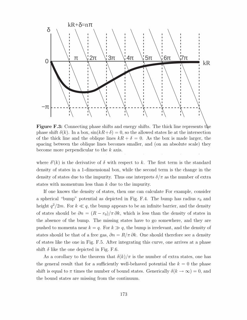
δ
0
−π
kRπ 2π 3π 4π 5π 6π 7π
kR+ =nδ π
Figure F.3: Connecting phase shifts and energy shifts. The thick line represents thephase shift δ(k). In a box, sin(kR+δ) = 0, so the allowed states lie at the intersectionof the thick line and the oblique lines kR + δ = 0. As the box is made larger, thespacing between the oblique lines becomes smaller, and (on an absolute scale) theybecome more perpendicular to the k axis.
where δ′(k) is the derivative of δ with respect to k. The first term is the standard
density of states in a 1-dimensional box, while the second term is the change in the
density of states due to the impurity. Thus one interprets δ/π as the number of extra
states with momentum less than k due to the impurity.
If one knows the density of states, then one can calculate For example, consider
a spherical “bump” potential as depicted in Fig. F.4. The bump has radius r0 and
height q2/2m. For k ≪ q, the bump appears to be an infinite barrier, and the density
of states should be ∂n = (R − r0)/π ∂k, which is less than the density of states in
the absence of the bump. The missing states have to go somewhere, and they are
pushed to momenta near k = q. For k ≫ q, the bump is irrelevant, and the density of
states should be that of a free gas, ∂n = R/π ∂k. One should therefore see a density
of states like the one in Fig. F.5. After integrating this curve, one arrives at a phase
shift δ like the one depicted in Fig. F.6.
As a corollary to the theorem that δ(k)/π is the number of extra states, one has
the general result that for a sufficiently well-behaved potential the k = 0 the phase
shift is equal to π times the number of bound states. Generically δ(k → ∞) = 0, and
the bound states are missing from the continuum.
173

xxxxxxxxxxxxxxxxxxxxxxxxxxxxxxxxxxxxxxxxxxxxxxxxxxxxxxxxxxxxxxxxxxxxxxxxxxxxxxxxxxxxxxxxxxxxxxxxxxxxxxxxxxxxxxxxxxxxxxxxxxxxxxxxxxxxxxxxxxxxxxxxxxxxxxxxxxxxxxxxxxxxxxxxxxxxxxxxxxxxxxxxxxxxxxxxxxxxxxxxxxxxxxxxxxxxxxxxxxxxxxxxxxxxxxxxxxxxxxxxxxxxxxxxxxxxxxxxxxxxxxxxxxxxxxxxxxxxxxxxxxxxxxxxxxxxxxxxxxxxxxxxxxxxxxxxxxxxxxxxxxxxxxxxxxxxxxxx
V(r)
q2
2m
r
Figure F.4: Energy states for a spherical bump in a box. States are pushed up bythe bump
Rπ
DOS
kq
R-rπ
Figure F.5: Density of states for a spherical bump in a box (schematic). Thepotential has a height of V0 = q2/2m, and width r.
kq
δ
Figure F.6: Phase shift for a spherical bump in a box (schematic). The height ofthe potential is q2/2m.
174
F.3 Sample phase shifts
In this section I plot a few illustrative phase shifts.
F.3.1 Hard wall
The simplest scattering potential is a hard wall:
V (r) =
∞ r < r0
0 r > r0.(F.30)
The wavefunction must vanish at the edge of the wall, so u(r) = sin(k(r − r0)) and
δ = −kr0. This example is pathological in that δ → ∞ as k → ∞.
F.3.2 Attractive well
A slightly more complicated simple potential is the attractive spherical well,
V (r) =
−V0 r < r0
0 r > r0.(F.31)
This potential is not realistic but it possesses many of the features of more sophis-
ticated atomic potentials. In particular there are low energy resonances whenever a
new bound state enters the well. To find the phase shifts I write the wavefunction as
u(r) =
A sin(k′r) r < r0
B sin(kr + δ) r > r0,(F.32)
where (k′)2/2m− V0 = k2/2m. Continuity of the wavefunction and its derivative are
guaranteed by matching the logarithmic derivative at r0, which gives
k′ cot(k′r0) = k cot(kr0 + δ). (F.33)
Solving for δ gives
tan δ =k sin k′r0 cos kr0 − k′ sin kr0 cos k′r0k′ cos k′r0 cos kr0 + k sin kr0 sin k′r0
. (F.34)
For different values of V0 I plot δ(k) in Fig. F.7. For simplicity I introduce the
momentum q, satisfying V0 = q2/2m, which marks the depth of the well. The most
striking feature of these graphs is that when cos(qr0) = 0, the phase shift at k = 0
jumps. This happens because a new bound state enters the well at this point.
175

δ
k/π0.5 1 1.5 2 2.5 3
0.5
1
1.5
2
2.5
3
Figure F.7: Phase shifts for a spherical well potential. The depth of the well isV0 = q2/2m and its radius is r0. All momenta are measured in terms of r0. Thevarious lines show different values of q, each differing by 0.1π/r0. Resonances occurat qr0 = (n+ 1/2)π.
176

0.5 1 1.5 2 2.5 3Hr0ΠL q
2.5
5
7.5
10
12.5
15
H2mR2Π2L E
Figure F.8: Energy levels for an attractive well of radius r0 and depth V0 = q2/2mwithin a box of size R. The energy is measured in terms of the quantization energyof the large box, π2/mR2. The horizontal axis shows qr0/π, a measure of the depthof the well. Resonances occur whenever qr0 = (n+ 1/2)π, and one of the continuumenergy states drops into the well. For this plot R = 50r0. Increasing R0 makes thejumps sharper.
It is instructive to put this system in a box of size R, and calculate the energy of
the first few levels as a function of q. As seen in Fig. F.8, whenever one passes through
a resonance, the lowest energy state becomes bound, and the next level replaces it.
What is happening is that each line has a fixed number of nodes, and at the resonance
one of the nodes moves from outside the well to inside the well, drastically reducing
the energy.
F.3.3 Resonant barrier
I next consider a resonant barrier potential, as shown in Fig. F.9,
V (r) =
0 r < r0
q2/2m r0 < r < 2r0
0 r > 2r0.
(F.35)
As opposed to the attractive well which possesses zero energy resonances, the resonant
barrier has finite energy resonances resulting from the quasi-bound states which are
177

V
r
q2
2m
r0 2r0
Figure F.9: Resonant barrier potential.
found at momenta where sin(kr0) ≈ 0. At these resonances, one finds an extra state.
From our understanding of δ′/π as the density of states, we should have a phase
change of π near this momentum. As seen in Fig. F.10, this is indeed the case.
F.4 The pseudopotential
Here I discuss an expansion of the scattering amplitude in powers of kr0, where r0 is
the length scale of the potential. This expansion takes the form
k cot δ = − 1
as+
1
2rek
2 + O((r0k)4). (F.36)
The parameters as and re are known as the scattering length and the effective range. I
emphasize that (F.36) is an expansion in r0k, and even when as is large, the remaining
terms can be small. The pseudopotential approximation amounts to taking only the
first term in this expansion.
One derives Eq. (F.36) via a matching argument. The Schrodinger equation
obeyed by u(r) = rψ(r) is(
k2 + ∂2r
2m− V (r)
)
u = 0. (F.37)
For r ≪ r0, V (r) dominates over k2, and one writes
u(r) = χ(r) + O(k2), r ≪ r0, (F.38)
where χ(r) is independent of k. For r ≫ r0, the potential V (r) vanishes and u takes
on its asymptotic form
u(r) = A sin(kr + δ), r ≫ r0. (F.39)
178

δ
k/π
0.5 1 1.5 2
-1
-0.8
-0.6
-0.4
-0.2
Figure F.10: Phase Shifts δ(k)/π for a resonant barrier potential. The momentumk is measured in units of π/r0. Each line corresponds to a different barrier height.
I match the logarithmic derivatives at r0, finding
k cot(kr0 + δ) = χ′/χ+ O(k2), (F.40)
which gives the desired expansion of k cot δ in powers of k2.
In terms of cot δ the scattering amplitude is
f =eiδ sin δ
k=
1
k cot δ + ik. (F.41)
So in the pseudo-potential approximation, the scattering amplitude is
f =−a
1 + ika. (F.42)
For small ak, this looks like a point interaction. For large values of ak, this looks like
a long-ranged 1/k potential.
179

a/r
qr10 20 30 40 50 60
-2
-1.5
-1
-0.5
0.5
1
1.5
2
Figure F.11: Scattering length a for a spherical well of radius r and depth V0 =q2/2m.
F.4.1 The pseudo-potential for an attractive spherical well
As an example, one can expand Eq. (F.34) in powers of k, finding
k cot δ =−1
as+rek
2
2(F.43)
as = r0 −tan qr0q
(F.44)
re = (1
q− r2
0q) cos qro + r0 sin qr0 +q2r3
0 cos2 qr0/3
sin qr0 − qr0 cos qr0. (F.45)
The effective range vanishes when as diverges. These quantities are plotted in Fig. F.11
and F.12.
F.5 Zero range potentials
For analytic calculations, the simplest potentials one can consider are zero-range
potentials. These play an important role in many theoretical works, so it is worth
considering them here. Zero range potentials are, by construction, singular. Thus,
despite their analytic simplicity, these potentials require taking careful limits.
180

re/r
qr20 40 60 80 100
-200
-100
100
200
300
400
Figure F.12: Effective range re for a spherical well of radius r and depth V0 = q2/2m.
F.5.1 A structureless point scatterer
Consider a point scatterer with a potential V (r) = V0δ(r− r′). In momentum space,
Vk = V0. Scattering off this potential is described by the T -matrix equation (F.17),
Tkk′(ω) = Vkk′(ω +∑
q
VkqG0(q)Tqk′(ω). (F.46)
Since Vkk′ is independent of the momentum indices, T will also be independent of
momentum. Using this result, the T -matrix is
T (ω) =V0
1 − V0Θ, (F.47)
where Θ is given by
Θ =∑
k
G0(q, ω) =∑
q
1
ω − q2/2m. (F.48)
Replacing the sum with an integral,
Θ =V
(2π)3
∫
d3q
ω − q2/2m(F.49)
=V
2π2
∫
dq q2
ω − q2/2m, (F.50)
181

one notices that the sum is ultraviolet divergent. This divergence is a consequence
of the short range of the potential, and reflects the fact that a point interaction is
unphysical. Any real potential will have a finite range, which will introduce a large q
cutoff, Λ in this integral. The integral is readily evaluated to be
Θ = Θ0 −imV
√2mω
2π(F.51)
Θ0 = −V mΛ
π2. (F.52)
The T -matrix is then of the form
T =2π
m
as
1 + ias
√2mω
, (F.53)
where the scattering length is
as ≡m
2π
V0
1 − V0Θ0
. (F.54)
Note that if one takes the cutoff Λ to infinity at fixed V0, then the scattering length
vanishes. In this sense, there is no scattering off a delta-function potential in three
dimensions. Only by scaling V0 with Λ can a non-zero as be produced. This scaling
of V0 with Λ is the simplest example of renormalization which can be discussed. As
previously discussed, a T -matrix of the form (F.53) gives a phase shift
δ = arg(T ) = − arctan(ask). (F.55)
F.5.2 Scattering from a zero-range bound state
A simple generalization of the structureless point scatterer is to associate a bound
state with the impurity. In such a case, the scattering is energy dependent, and
Vk = V0 +|α|2ω − ǫ
, (F.56)
where V0 is a static potential at the origin, α is an amplitude for entering the bound
state, and ǫ is the energy of the bound state. To illustrate the role of the bound state
I set V0 = 0, in which case
T =|α|2
ω −E + i(m/2π)|α|2√
2mω. (F.57)
The energy E is
E = ǫ+ |α|2Θ0. (F.58)
182
For E to be finite as Λ → ∞ one must scale ǫ with Θ0.
The T -matrix (F.57) leads to a phase shift of the form
cot(δ) = − 1
ask+ reffk
2/2, (F.59)
where
as =−m|α|2
2πE(F.60)
reff =−2π
m2|α|2 . (F.61)
A resonance occurs when E = 0.
The Green’s function for the bound state is T/|α|2. Thus E is the energy of the
bound. When E > 0, this state has a finite lifetime
1
τ=m
2π|α|2
√2mE, (F.62)
which is the result one would expect from Fermi’s golden rule.
F.6 Feshbach resonances
As is clear from the above examples, tuning a resonance near zero energy has dramatic
consequences for atomic scattering properties. Experimentally such tuning is carried
out by applying magnetic fields. The field induced resonance is known as a Feshbach
resonance.
The underlying principle is that due to the hyperfine interaction, two colliding
atoms can form a bound state whose magnetic moment is not equal to the sum of the
magnetic moments of the incoming atoms (total angular momentum is conserved, not
total magnetic moment). Consequently, when a magnetic field is applied, the Zeeman
shift of the bound state can be different from the shift of the scattering states. Thus
the energy of the bound state is tunable. When its energy is set to zero one is at
the resonance. The scattering properties near the resonance are described well by the
model of Section F.5.2.
F.7 Multiple scattering
I now turn to the question of scattering off several small impurities which are much
farther apart than the range of their potentials. As detailed in Section F.4, low energy
183

scattering off an individual impurity is described by the scattering length as. Letting
n denote the density of scatterers, I am particularly interested in the limit where na3s
is of order 1. In this limit one encounters localization effects, and the scattering off
of one impurity depends on the presence of all others.
F.7.1 Elementary approach
In this Section I frame the problem in terms of elementary quantum mechanics.
Imagine that one has static impurities at positions r1, r2, . . . , rn. The phase shifts
for scattering off any of these impurities is δ0(k). In a scattering experiment, the
asymptotic wavefunction will be
ψ(r) = eikz +∑
i
fieik|r−ri|
|r − ri|, (F.63)
where the fi’s will be independent of space. This wavefunction should be good, except
on atomic distances close to individual impurities. Comparing with Eq. (F.1), the
scattering amplitude for scattering from the collection of impurities is
f(k, r) =∑
i
fieikri ·r. (F.64)
The s-wave component of this scattering amplitude is
fs(k) =
∫
dΩ
4πf(k) =
∑
i
fisin kri
kri. (F.65)
In particular, when kri ≪ 1 then
fs(k) =∑
i
fi. (F.66)
My goal is to calculate the phase shift δ given by
fs =eiδ sin δ
k. (F.67)
I now determine the fi’s via the restriction that at each impurity, the phase shift
is δ0. Once we know fi we know f . Near the ith impurity, the spherically symmetric
part of ψ is defined by
ψ(s)i (|r − ri|) =
∫
dΩ′
4πψ(r = r′ + ri), (F.68)
184

where dΩ′ is a solid angle with respect to the variable r′, which is centered at the
impurity. The integration is straight forward and one finds
ψ(s)i (r − ri) =
(
eikzi +∑
j,j 6=i
fjeik|ri−rj |
|ri − rj|
)
sin k|r − ri|k|r − ri|
+ fieik|r−ri|
|r − ri|. (F.69)
I will use the symbol Ai for the term in large parentheses. We know that this term
must have the form
ψ(s)i (r − ri) =
sin(k|r − ri| + δ0)
k|r − ri|. (F.70)
Equating these two expressions, one arrives at
fi = Aieiδ0 sin δ0
k. (F.71)
Using this expression in the definition of Ai one finds that Ai satisfies the following
matrix equation,(
δij − eiδ0 sin δ0eik|ri−rj |
k|ri − rj|
)
Aj = eikzj . (F.72)
I denote the matrix on the left hand side of this equation by 1−g. Formally inverting
this matrix gives
A1
...
An
=1
1 − g
eikz1
...
eikzn
. (F.73)
The total scattering amplitude f is then
f(k, k, r) =eiδ0 sin δ0
k
(
e−ikr·r1 · · · e−ikr·rn) 1
1 − g
eikk·r1
...
eikk·rn
(F.74)
=eiδ0 sin δ0
k
∑
ij
eik(k·ri−r·rj)(
1
1 − g
)
ij
. (F.75)
Formally we are now done. If kri ≪ 1 we neglect the eikri’s and get
eiδ sin δ = eiδ0 sin δ0∑
ij
(
1
1 − g
)
ij
. (F.76)
In this same approximation
gij =
eiδ0 sin δ0k|ri−rj | i 6= j
0 i = j.. (F.77)
185
In the pseudo-potential approximation,
eiδ0 sin δ0 =−ask
1 + iask. (F.78)
It is useful to study the structure of (1−g)−1. The matrix g has the property that
gij is a function only of the distance |ri − rj |, and is essentially a scattering ampli-
tude times a propegator. One graphically thinks of gij as a directed line connecting
impurity i to impurity j. Then ((1− g)−1)ij is the sum over all paths connecting i to
j.
F.7.2 T-matrix approach
With less work (but using more machinery) one can derive the results as the last
Section by directly calculating the T -matrix, defined by
T = V + V1
H0 −ET. (F.79)
In the present case, V =∑
i Vi is the sum of the potentials for each scatterer. If one
defines Ti as the sum of scattering off an individual impurity,
Ti = Vi + Vi1
H0 −ETi, (F.80)
then T is given by a sum over all paths between scatters of Ti’s with propegators
between them,
T =∑
i
Ti +∑
i6=j
Ti1
H0 − ETj + · · · , (F.81)
=∑
i
Ti +∑
ij
Ti(1 − δij)1
H0 −ETj + · · · . (F.82)
I introduce a matrix Gij by
Gij = (1 − δij)1
H0 − ETj , (F.83)
so that the T-matrix is formally
T =∑
ij
Ti
(
1
1 −G
)
ij
. (F.84)
To go any farther one needs to choose a basis. The most convenient basis for
the current problem is in momentum space. If we treat the Ti’s within the pseudo-
potential approximation, then
Ti(k, k′, q) = 〈k′|Ti(E = q2/2m)|k〉 = ei(k−k′)ri
(−2π
mqeiδ0 sin δ0
)
. (F.85)
186
For notational simplicity, I use the symbol x for the parentheses. The operator
Ti(H0 −E)−1Tj is evaluated by inserting a resolution of the identity
〈k′|Ti(H0 − E)−1Tj |k〉 =
∫
d3k
(2π)3T (k, k, q)
2m
k2 − q2T (k, k′, q) (F.86)
= x2ei(krj−k′ri)m
2π
eiq|ri−rj |
q|ri − rj |. (F.87)
In Eq. (F.81) all of the eikri ’s cancel, except for the one at the end and the one at the
beginning. Thus T is given by
T (k, k′, q) = x∑
ij
ei(kri−k′rj)Mij(q), (F.88)
where Mij(q) is the sum of all paths going from i to j, each segment of the path going
from impurity µ to impurity ν contributing x(m/2π)eiq|rµ−rν |/(q|rµ − rν |), which is
readily seen to be identical to (F.75).
F.7.3 Two scatterers
Given the positions r1, r2, . . . , rn of the scatterers we can now calculate δ in terms
of δ0. The simplest example of this procedure uses two scatterers. The matrix gij is
given by
g =
(
0 x
x 0
)
(F.89)
x =eik|r1−r2|
k|r1 − r2|sin δ0e
iδ0 (F.90)
≈ −as(1 + ikr)/r
1 + ikas, (F.91)
where r ≡ |r1 − r2| and as is the scattering length for scattering off a single impurity.
Since g is proportional to a Pauli matrix, g2 = x2 is proportional to the identity.
Thus (1 − g)−1 is (1 − x2)−1(1 + g). The scattering amplitude is then
f =eiδ0 sin δ0
k
∑
ij
(
1
1 − g
)
ij
(F.92)
=eiδ0 sin δ0
k
1
1 − x2(2 + 2x) (F.93)
=−(
2as
1+as/r
)
1 + i(
2as
1+as/r
)
k. (F.94)
187

The last line follows from some simple algebraic rearrangements. The end result is
that the scattering from two impurities looks like scattering from a single one with
an effective scattering length
a2 =2as
1 + as/r. (F.95)
For as ≪ r the scattering is just additive. For as ≫ r the effective scattering length
is cut off by the distance between the two impurities, and a2 → 2r.
It should be clear from this result that when particles are packed closer than their
scattering lengths one cannot consider the scattering from each particle independently.
F.7.4 Low density limit
In the low density limit, na3s ≪ 1, the matrix elements gij are small, and the single
scattering dominates. The phase shift for scattering off the collection of impurities is
then additive, δ = Nδ0.
F.8 Scattering in the many body problem
This thesis is concerned with clouds of interacting atoms, described via a density n and
scattering length as. In the dilute limit na3s ≪ 1, multiple scattering is suppressed,
and the interaction can be treated perturbatively (see Chapter 2 and Appendix E).
Most alkali gas experiments are in this regime. By using Feshbach resonances one
should be able to tune the scattering length so that na3s is no longer small. Un-
derstanding this strongly interacting regime is a major challenge facing the cold gas
community.
188

References
[1] M. H. Anderson, J. R. Ensher, M. R. Matthews, C. E. Wieman, and E. A.Cornell, Science 269, 198 (1995).
[2] K. B. Davis, M.-O. Mewes, M. R. Andrews, N. J. van Druten, D. S. Durfee, D.M. Kurn, and W. Ketterle, Phys. Rev. Lett. 75, 3969 (1995).
[3] C. C. Bradley, C. A. Sackett, J. J. Tollett, and R. G. Hulet, Phys. Rev. Lett.75, 1687 (1995).
[4] M. Toda, R. Kubo, and N. Saito Statistical physics, Springer-Verlag, 1991.
[5] N. Wilkin, J. Gunn, and R. Smith, Phys. Rev. Lett. 80, 2265 (1998).
[6] P. Nozieres, in Bose-Einstein Condensation, edited by A. Griffin, D. W. Snoke,and S. Stringari (Cambridge University Press, 1995).
[7] T.-L. Ho and S. K. Yip, Phys. Rev. Lett. 84, 4031 (2000).
[8] R. Bowers, and T. Deeming Astrophysics II; Interstellar Matter and Galaxies(Jones and Bartlett, Sudbury, MA, 1984).
[9] H.-J. Miesner, D. M. Stamper-Kurn, J. Stenger, S. Inouye, A. P. Chikkatur,and W. Ketterle, Phys. Rev. Lett. 82, 2228 (1999).
[10] K. W. Madison, F. Chevy, W. Wohlleben, J. Dalibard, Phys. Rev. Lett. 84,806 (2000).
[11] C. Liu, Z. Dutton, C. H. Behroozi, L. V. Hau, Nature 409, 490 (2001).
[12] D. F. Phillips, A. Fleischhauer, A. Mair, R. L. Walsworth, and M. D. Lukin,Phys. Rev. Lett. 86, 783 (2001).
[13] F. Dalfovo, S. Giorgini, L. P. Pitaevskii, and S. Stringari, Rev. Mod. Phys. 71,463 (1999).
[14] C. J. Pethick and H. Smith, Bose-Einstein Condensation in Dilute Gases (Cam-bridge University Press, to be published).
[15] A. S. Parkin and D. F. Walls, Phys. Rep. 303, 1 (1998).
[16] A. J. Leggett, Rev. Mod. Phys. 73, 307 (2001).
189
[17] E. Cornell, J. Res. Nat. Inst. Stand. Technol. 101, 419 (1996).
[18] G. Baym and C. J. Pethick, Phys. Rev. Lett. 76, 6 (1996).
[19] D. G. Fried, T. C. Killian, L. Willmann, D. Landhuis, S. C. Moss, D. Kleppner,and T. J. Greytak, Phys. Rev. Lett. 81, 3811 (1998).
[20] F. P. Dos Santos, J. Leonard, J. Wang, C. J. Barrelet, F. Perales, E. Rasel, C.S. Unnikrishnan, M. Leduc and C. Cohen-Tannoudji, Phys. Rev. Lett. 86, 3459(2001).
[21] A. Robert, O. Sirjean, A. Browaeys, J. Poupard, S. Nowak, D. Boiron, C. I.Westbrook, A. Aspect Science 292, 461 (2001).
[22] A. G. Truscott, K. E. Strecker, W. I. McAlexander, G. Partridge,and R. G. Hulet, Science 291, 2570 (2001); B. DeMarco and D. S.Jin, Science 285, 1703-1706 (1999); J. Cubizolles , F. Schreck , K.Corwin , L. Khaykovich, G. Ferrari, C. Salomon, in preparation (seehttp://www.lkb.ens.fr/recherche/atfroids/anglais/lithium.html)
[23] M. R. Andrews, C. G. Townsend, H.-J. Miesner, D. S. Durfee, D. M. Kurn, andW. Ketterle, Science 275, 637 (1997).
[24] C.A. Sackett, H.T.C. Stoof, and R.G. Hulet, Phys. Rev. Lett. 80 2031, (1998);C.A. Sackett, C.C. Bradley, M. Welling, and R.G. Hulet, Appl. Phys. B 65 433,(1997); C.C. Bradley, C.A. Sackett, and R.G. Hulet, Phys. Rev. Lett. 78 985,(1997); C.C. Bradley, C.A. Sackett, and R.G. Hulet, Phys. Rev. A 55 3951,(1997).
[25] J. L. Roberts, N. R. Claussen, S. L. Cornish, E. A. Donley, E. A. Cornell, andC. E. Wieman, Phys. Rev. Lett. 86, 4211 (2001); S. L. Cornish, N. R. Claussen,J. L. Roberts, E. A. Cornell, and C. E. Wieman, preprint, cond-mat/0004290.
[26] C.A. Sackett, H.T.C. Stoof, and R.G. Hulet, Phys. Rev. Lett. 80 2031, (1998);Yu. Kagan, A.E. Muryshev, and G.V. Shlyapnikov, Phys. Rev. Lett. 81, 933,(1998).
[27] P.A. Ruprecht, M.J. Holland, K. Burnett, and M. Edwards, Phys. Rev. A 51,4704 (1995).
[28] S. L. Cornish, N. R. Claussen, J. L. Roberts, E. A. Cornell, and C. E. Wieman,Phys. Rev. Lett. 85 1795 (2000); J. L. Roberts, N. R. Claussen, J. P. Burke,Jr., C. H. Greene, E. A. Cornell, and C. E. Wieman, Phys. Rev. Lett. 81 5109(1998); S. Inouye, M. R. Andrews, J. Stenger, H.-J. Miesner, D. M. Stamper-Kurn, W. Ketterle, Nature 392 151 (1998).
[29] A. Einstein Sitzungsber. Kgl. Preuss. Akad. Wiss. 1925, 3 (1925).
[30] P. Gruter, D. Ceperley, and F. Laloe, Phys. Rev. Lett. 79, 3549 (1997).
190
[31] T. Toyoda, Ann. Phys. (N.Y.) 141, 154 (1982); K. Huang, in Studies in Sta-tistical Mechanics (North- Holland, Amsterdam, 1964), Vol. II; H. T. C. Stoof,Phys. Rev. A 45, 8398 (1992); M. Bijlsma and H. T. C. Stoof, Phys. Rev. A 54,5085 (1996).
[32] G. Baym, J.-P. Blaizot, M. Holzmann, F. Laloe and D. Vautherin, Phys. Rev.Lett. 83 1703 (1999).
[33] G. Baym, J.-P Blaizot, J. Zinn-Justin, Europhys. Lett. 49, 150 (2000).
[34] J. R. Ensher, D. S. Jin, M. R. Matthews, C. E. Wieman, and E. A. Cornell,Phys. Rev. Lett. 77, 4984 (1996).
[35] E. J. Mueller, G. Baym, and M. Holzmann, accepted for publication J. Phys. B;At. Mol. Opt. Phys (2001).
[36] N. Goldenfeld Lectures on phase transitions and the renormalization group,(Addison-Wesley, Reading, Massachusetts, 1992).
[37] M. Holzmann and W. Krauth, Phys. Rev. Lett. 83, 2687 (1999).
[38] M. Wilkens, F. Illuminati, and M. Kramer, J. Phys. B: At. Mol. Opt. Phys. 33(2000) L779 (2000).
[39] P. Arnold and G. Moore, cond-mat/0103228 (2001).
[40] V. Kashurnikov, N. Prokof’ev N, and B. Svistunov, cond-mat/0103149 (2001).
[41] G. Baym and C. Pethick Landau Fermi liquid theory: concepts and applications,(J. Wiley and Sons, New York, 1991).
[42] Illuminati F, Navez P, and Wilkens M 1999 J. Phys. B: At. Mol. Opt. Phys.32, L461.
[43] S. Giorgini, L. P. Pitaevskii, and S. Stringari, Phys. Rev. A 54, 4633 (1996).
[44] P. Arnold and B. Tomasik, cond-mat/0105147.
[45] O. Penrose, Phil. Mag. 42, 1373 (1951).
[46] O. Penrose and L. Onsager, Phys. Rev. 104, 576 (1956).
[47] P. Nozieres and D. Saint James, J. Physique 43, 1133 (1982).
[48] M. Girardeau, Phys. Fluids 5, 1468 (1962).
[49] F. Pollock, Phys. Fluids 10, 473 (1967).
[50] E. J. Mueller, T.-L. Ho, G. Baym, and M. Ueda, to be submitted to PhysicalReview A (2001).
[51] H. G. Vaidya and C. A. Tracy, Phys. Rev. Lett. 42, 3 (1979).
191

[52] P. C. Hohenberg and P. C. Martin, Ann. Phys. 34, 291 (1965).
[53] Yu. Kagan, V. A. Kashurnikov, A. V. Krasavin, N. V. Prokof’ev, and B. V.Svistunov, Phys. Rev. A 61, 043608 (2000); J. M. Kosterlitz and D. J. Thouless,J. Phys. C 6 1181 (1973).
[54] D.S. Petrov, G.V. Shlyapnikov, and J.T.M. Walraven cond-mat/0104373.
[55] Yu. Kagan and B. V. Svistunov Phys. Rev. Lett. 79, 3331 (1997).
[56] C. N. Yang, Rev. Mod. Phys. 34, 694 (1963).
[57] W. Kohn and D. Sherrington, Rev. Mod. Phys. 42, 1 (1970).
[58] I. Zapata, F. Sols, and A. J. Leggett, Phys. Rev. A. 57, R28 (1998).
[59] Y. Castin and C. Herzog, “Bose-Einstein condensates in symmetry breakingstates”, Lecture Notes of the Cargese School on Bose-Einstein condensates (July2000); reprinted as cond-mat/0012040.
[60] J. Javanainen and S. M. Yoo, Phys. Rev. Lett. 76, 161 (1996).
[61] Y. Castin and J. Dalibard, Phys. Rev. A 50, 4330 (1997).
[62] D. M. Stamper-Kurn, M. R. Andrews, A. P. Chikkatur, S. Inouye, H. J. Miesner,J. Stenger, and W. Ketterle, Phys. Rev. Lett. 80, 2027 (1998).
[63] C. K. Law, H. Pu, and N. P. Bigelow, Phys. Rev. Lett. 81, 5257 (1998).
[64] M. Koashi and M. Ueda, Phys. Rev. Lett. 84, 1066 (2000).
[65] T.-L. Ho, Phys. Rev. Lett. 81, 742 (1998); T. Ohmi and K. Machida, J. Phys.Soc. Jpn. 67, 1822 (1998).
[66] N. Bogoliubov, J. Phys. 11, 23 (1947).
[67] M. Ueda, Phys. Rev. A 63, 013601 (2001).
[68] J. Javanainen, J. Phys. B 33, 5493 (2000).
[69] W.-J. Huang, Phys. Rev. A 63, 015602 (2000).
[70] C.J. Pethick and L. Pitaevski, Phys. Rev. A 62, 033609 (2000).
[71] N. Mermin and H. Wagner, Phys. Rev. Lett. 17, 1133 (1966).
[72] M. Ueda and A. J. Leggett, Phys. Rev. Lett. 83, 1489 (1999).
[73] Y. Lyanda-Geller and P. M. Goldbart, Phys. Rev. A 61, 043609 (2000).
192

[74] B. P. Anderson and M. A. Kasevich in Proceedings of the International School ofPhysics ’Enrico Fermi’, Course CXL, Bose-Einstein Condensation in AtomicGases, (M. Inguscio, S. Stringari, and C. E. Wieman, Eds., IOS Press, Amster-dam, 1999), pp. 439-452.
[75] M. P. A. Fisher, P. B. Weichman, G. Grinstein, D. S. Fisher, Phys. Rev. B 40,546 (1988).
[76] D. Van Oosten, P. Van der Straten, and H. T. C. Stoof, Phys. Rev. A 63,053601 (2001).
[77] C.J. Myatt, E.A. Burt, R.W. Ghrist, E.A. Cornell and C.E. Wieman. Phys.Rev. Lett. 78, 586 (1997), H.-J. Miesner, D. M. Stamper-Kurn, J. Stenger, S.Inouye, A. P. Chikkatur, and W. Ketterle, Phys. Rev. Lett. 82, 2228 (1999).
[78] B. D. Esry, Phys. Rev. A, 58, 3399 (1998).
[79] B. D. Esry, and C. H. Greene, Phys. Rev. A, 59, 1457 (1999).
[80] M. R. Matthews, B. P. Anderson, P. C. Haljan, D. S. Hall, C. E. Wieman, andE. A. Cornell, Phys. Rev. Lett. 83, 2498 (1999).
[81] G. Baym, Phys. Rev. B 51, 11697 (1995).
[82] J. R. Abo-Shaeer, C. Raman, J. M. Vogels, W. Ketterle, Science, 292, 476(2001).
[83] G. J. Milburn, J. Corney, E. M. Wright, and D. F. Walls, Phys. Rev. A 55,4318(1997).
[84] R. W. Spekkens and J. E. Sipe, Phys. Rev. A 59, 3868 (1999).
[85] E. J. Mueller, P. Goldbart and Y. Lyanda-Geller, Phys. Rev. A 57, 1505 (1998)
[86] W. A. Little, Phys. Rev. 156, 396 (1967).
[87] J. Langer and V. Ambegaokar, Phys. Rev. 164, 498 (1967).
[88] D. McCumber and B. Halperin, Phys. Rev. B 1, 1054 (1970).
[89] See also M. Tinkham, Introduction to Superconductivity (McGraw-Hill, NY,1975), Chap. 7.
[90] D. S. Rokhsar, Phys. Rev. Lett. 79, 2164 (1997); D. S. Rokhsar, cond-mat/9709212.
[91] Y. Lyanda-Geller and P. M. Goldbart, Phys. Rev. A 61, 3609 (2000); M. Nishidaand S. Kurihara, J. Phys. Soc. Jpn. 68, 3778 (1999); K. G. Petrosyan, and L.You, Phys. Rev. A 59, 639 (1999); M. Benakli, S. Raghavan, A. Smerzi, S.Fantoni, and S. R. Shenoy, Europhys. Lett. 46, 275 (1999); L. D. Carr, C. W.Clark, W. P. Reinhard, Phys. Rev. A 62, 3610 (2000); L. Salasnich, A. Parola,L. Reatto, Physical Review A, vol. 59, 2990-2995 (1999).
193

[92] M.R. Matthews, B.P. Anderson,P.C. Haljan, D.S. Hall, C.E.Wieman, E.A. Cor-nell, Phys. Rev. Lett. 83, 2498 (1999), B. P. Anderson, P. C. Haljan, C. E.Wieman, E. A. Cornell, Phys. Rev. Lett. 85, 2845 (2000).
[93] E. M. Wright, J. Arlt, and K. Dholakia, Phys. Rev. A, 63, 013608 (2001)
[94] G. Birkl, F. B. J. Buchkremer, R. Dumke, and W. Ertmer, Opt. Comm. 191, 67(2001); J. Reichel, W. Hansel, P. Hommelhoff and T. W. Hansch, Appl. Phys.B 72, 81-89, (2000).
[95] J. S. Langer and M. E. Fisher, Phys. Rev. Lett. 19, 560 (1967); R. J. Donnelly,Quantized Vortices in Helium II (Cambridge University Press, 1991), Chap. 8.
[96] J. E. Williams, M. J. Holland Nature 401, 568(1999).
[97] M. R. Andrew, K. M. Kurn, H.-J. Miesner, D. S. Durfee, C. G. Townsend, S.Inouye, and W. Ketterle, Phys. Rev. Lett. 79, 553 (1997)
[98] E. J. Mueller and G. Baym, Phys. Rev. A 62, 053605 (2000).
[99] P.A. Ruprecht, M.J. Holland, K. Burnett, and M. Edwards, Phys. Rev. A 51,4704 (1995).
[100] M. J. Davis, D. A. W. Hutchinson, and E. Zaremba, J. Phys. B 32, 3993 (1999);T. Bergeman, Phys. Rev. A 55, 3658 (1997); M. Houbiers and H. T. C. Stoof,Phys. Rev. A 54, 5055 (1996); P.A. Ruprecht, M.J. Holland, K. Burnett, andM. Edwards, Phys. Rev. A 51, 4704 (1995).
[101] J. Tempere, F. Brosens, L. F. Lemmens and J. T. Devreese, Phys. Rev. A, 61,043605 (2000).
[102] H. Saito and M. Ueda, preprint cond-mat/0006410; Yu. Kagan, A. E. Mury-shev, and G. V. Shlyapnikov, Phys. Rev. Lett. 81, 933 (1998); 79, 2670 (1996);also see the experiments in Ref. [24, 25].
[103] C. Huepe, S. Metens, G. Dewel, P. Borckmans, and M. E. Brachet, Phys. Rev.Lett. 82, 1616 (1999); M. Ueda and A. J. Leggett, Phys. Rev. Lett. 80, 1576(1998); Yu. Kagan, G. V. Shlyapnikov, and J. T. M. Walraven, Phys. Rev. Lett.81, 933 (1998); H. T. C. Stoof, J. Stat. Phys. 87, 1353 (1997).
[104] A. Griffin, Excitations in a Bose-Condensed Liquid (Cambridge UniversityPress, Cambridge, 1993).
[105] N.N. Bogoliubov, J. Phys. USSR, 11, 23 (1947).
[106] N.D. Mermin, Ann. Phys. 18, 421, 454 (1962); 21, 99 (1963).
[107] P. Szepfalusy and I. Kondor, Ann. Phys. 82, 1 (1974).
[108] A. Minguzzi and M. P. Tosi, J. Phys: Condens. Matter 9, 10211 (1997).
194

[109] G. Baym, Phys. Rev. 127, l39l (1962).
[110] A. J. Moerdijk, H. M. J. M. Boesten, and B. J. Verhaar, Phys. Rev. A 53, 916(1996); C. A. Sackett, J. M. Gerton, M. Welling, and R. G. Hulet, Phys. Rev.Lett. 82, 876 (1999).
[111] J. Bardeen, L. N. Cooper, and J. R. Schrieffer, Phys. Rev. 108, 1175 (1957).
[112] H. T. C. Stoof, Phys. Rev. A 49, 3824 (1994).
[113] L.P. Kadanoff and G. Baym, Quantum Statistical Mechanics (W.A. Benjamin,New York, 1962).
[114] T. Isoshima, K. Machida, and T. Ohmi, Phys. Rev. A 60, 4857 (1999).
[115] For a similar theoretical account, see P. Ao, and S. T. Chui, J. Phys. B 33, 535(2000).
[116] T.-L. Ho, Phys. Rev. Lett. 81, 742 (1998).
[117] Similar excitation spectra are found in E.V. Goldstein and P. Meystre, Phys.Rev. A 55, 2935 (1997).
[118] J. W. Kane and L. P. Kadanoff, J. Math. Phys. 6, 1902 (1965).
[119] A. Griffin in Proceedings of the International School of Physics ’Enrico Fermi’,Course CXL, Bose-Einstein Condensation in Atomic Gases, (M. Inguscio, S.Stringari, and C. E. Wieman, Eds., IOS Press, Amsterdam, 1999), edited byM.Inguscio, S.Stringari and C. Wieman (Italian Physical Society,1999); cond-mat/9901172.
[120] M. Imamovic-Tomasovic and A. Griffin, Journ. of Low Temperature Physics,122, 617 (2001); T. Nikuni and A. Griffin, Phys. Rev. A63, 033608-033628(2001); M. Imamovic-Tomasovic and A. Griffin, in Recent Progress in Non-Equilibrium Green’s functions, ed. by M. Bonitz (World Scientific, Singapore,2000), p.404-417; A. Griffin, in Bose-Einstein Condensation: From atomicphysics to quantum liquids, ed. by C.M. Savage and M. Das (World Scientific,Singapore, 2001); E. Zaremba, T. Nikuni and A. Griffin, Journ. Low Temp.Phys., 116, 277 (1999); Milena Imamovic-Tomasovic and Allan Griffin, Phys.Rev. A60, 494 (1999).
[121] R. Walser, J. Williams, J. Cooper, M. Holland Phys. Rev. A 59, 3878 (1999).
195

[122] C. W. Gardiner and P. Zoller, Phys. Rev. A, 55, 2902 (1997); D. Jaksch, C.W. Gardiner, and P. Zoller, Phys. Rev. A. 55, 575 (1997); C. W. Gardiner,Phys. Rev. A 56, 1414 (1997); C. W. Gardiner, P. Zoller, R. Ballagh, and M.J. Davis, Phys. Rev. Lett. 79, 1793 (1997); D. Jaksch, C. W. Gardiner and P.Zoller, Phys. Rev. A. 56, 575 (1997); C. W. Gardiner, P. Zoller, Phys. Rev. A58, 536 (1998); D. Jaksch, C. W. Gardiner, K. M. Gheri and P. Zoller Phys.Rev. A 58, 1450 (1998); C. W. Gardiner M. D. Lee, R. J. Ballagh, M. J. Davisand P. Zoller, Phys. Rev. Lett. 81, 5266 (1998) ; C. W. Gardiner and P. Zoller,Phys. Rev. A 61, 033601 (2000); M. D. Lee and C.W. Gardiner, Phys. Rev. A62, 033606 (2000); M. J. Davis, C. W. Gardiner and R. J. Ballagh, Phys. Rev.A 62, 063608 (2000);
[123] U. Al Khawaja and H. T. C. Stoof Phys. Rev. A 62, 53602 (2000).
[124] S. L. Cornish, N. R. Claussen, J. L. Roberts, E. A. Cornell, C. E. Wieman,Phys. Rev. Lett. 85, 1795 (2000); S. L. Cornish, N. R. Claussen, J. L. Roberts,C. E. Wieman, Phys. Rev. Lett. 85, 728 (2000). S. Inouye, M.R. Andrews, J.Stenger, H.-J. Miesner, D.M. Stamper-Kurn, and W. Ketterle, Nature 392, 151(1998).
[125] J. Glanz, New York Times (Jan. 18, 2001).
[126] B. V. Svistunov and G. V. Shlyapnikov, Sov. Phys. JETP 70, 460 (1990); 71,71 (1990).
[127] R. M. Ziff, G. E. Uhlenbeck, and M. Kac, Phys. Rep. 32, 169 (1977).
[128] Robinson, Phys. Rev. 83, 678 (1951).
[129] Titchmarsh, The theory of the Riemann Zeta-Function, Oxford UniversityPress, 1951.
[130] Whittaker and Watson, Modern Analysis, Cambridge University Press, 1947.
[131] Morse and Feshbach, Methods of theoretical physics, Technology Press, 1946.
[132] N.D. Mermin, Ann. Phys. 18, 421 (1962); 454 (1962); 21,99 (1963).
[133] G. Mahan, Many-Particle Physics, Plenum Press, New York, 1981.
[134] J. Shumway and D. M. Ceperley, cond-mat/9907309.
196
Index
angular momentum, 51–55, 72, 74, 75,78
Bernoulli numbers, 126Bethe ansatz, 55Bogoliubov, 51, 52, 62, 103–105Boltzmann equation, 97, 153, 154boson Hubbard model, 56
coherence, 39experiments, 12length, 1, 70, 72, 98, 99
collapse, 2, 80–95experiment, 12
collision integral, 97, 101collisions, 105, 110, 115commensurability, 48conservation laws, 102, 104, 105, 145–
151cooling
Doppler, 4evaporative, 6
degeneracy, 2, 44, 48, 49, 56, 64density matrix
single particle, 40, 43, 50, 53, 57–59, 62, 64–66, 68
two particle, 50density of states, 21, 22, 130dipole, 114dissipation, 2divergences
infrared, 1, 20, 21, 31, 35, 130ultraviolet, 182
Doppler broadening, 115, 122
electromagnetically induced transparency,3, 16, 112–124
energy barrier, 55
experiment, 3–17coherence, 12collapse, 12cooling and trapping, 4–9electromagnetically induced trans-
parency, 16fermions, 11Feshbach resonance, 16helium, 11hydrogen, 11interference, 12, 46–48measurement, 9–11
atom detection, 11imaging, 10spectroscopy, 11
spin, 16
Fermi pressure, 81fermions, 11Feshbach resonance, 16, 105, 166, 183
experiment, 16finite size scaling, 20, 23–31fragmentation, 2, 39–68, 79free energy, 20–23, 29–32, 34, 73, 129–
136
Green’s function, 97–99, 102, 103, 112,119, 120, 124, 137, 142
Gross Pitaevskii equation, 70, 143
Hartree Fock, 85Hartree-Fock, 86
interactionsstrong, 18
Jeans instability, 80Josephson array, 56Josephson junction, 42, 61–65
197

asymmetric, 49, 63–65experimental parameters, 45regimes, 44
Josephson plasma frequency, 44
kinetics, 3, 72, 96–105
lithium, 12, 80–82, 87, 89, 90, 92local density approximation, 83localization, 45, 49, 56–58
Matsubara frequencies, 163measurement
experiment, 9fragmentation, 46–48phase slips, 78
Mellin transform, 127, 130metastability, 15, 69, 72, 73, 77, 81, 93microchannel plate, 11Monte-Carlo, 18
one dimensional gas, 54, 55optical lattices, 56optical molasses, 4
pairing, 2, 80, 91partition function, 20persistent currents, 2, 69–79perturbation theory, 18, 31–35phase diagram, 81, 82phase shifts, 170–171phase slip, 2, 69–79phase transition
BEC, 1, 18–37dimensionality, 21
liquid-gas, 85, 156localization-delocalization, 56
photons, 16, 112–115Poisson brackets, 99polaritons, 16, 112–124
dark, 116polarons, 16, 112, 117, 119, 124polylogarithm, 22, 26, 86, 126–129pseudo-potential, 178
quantum pressure, 81, 107quasicondensate, 41
quasiparticle, 96, 102, 104
random phase approximation, 85, 156rubidium, 12, 37, 77, 80–82, 87, 89, 90,
92, 115
scattering, 166–188multiple, 183resonances, 166
scattering amplitude, 166Schrodinger Cat, 65self-energy, 98, 120, 122, 146, 148sodium, 4, 115soliton, 55spectral density, 103, 109spin
fragmentation, 49–52phase separation, 2, 16textures, 55Zeeman splitting, 6
spin:phase separation, 93spinodal, 156squeezed states, 48Stern Gerlach experiment, 52Stirling numbers, 134sum rules, 141superfluidity, 2, 69symmetry breaking, 39–68sympathetic cooling, 12
T-matrix, 164, 167–169, 170, 186–187thermal activation, 72thermal pressure, 81trapping, 4, 83, 89two level model, 42–45, 55
uncertainty principle, 4
vortex, 52, 59, 60, 78
zero sound, 157zeta function, 22, 126
spectral, 131, 132
198

Vita
Erich Jon Mueller was born September 27, 1974, in Calgary, Canada. In 1996, herecieved an honours B.Sc. in mathematics and physics from the University of BritishColumbia in Vancouver, Canada; graduating top of his class. At UBC he studiedboth experimental and theoretical physics, first working with semiconductor quantumwells in the experimental laboratory of Jeff Young, then writing an undergraduatethesis on quantum measurement under the direction of Philip Stamp. Following hisundergraduate studies, he spent five years studying quantum degenerate gases withGordon Baym at the University of Illinois at Urbana-Champaign, earning his Ph.D.in theoretical physics in 2001. He is currently working with Tin-Lun Ho at the OhioState University in Columbus, Ohio. His publications include:
E.J. Mueller, G. Baym, and M. Holtzmann, “Finite size scaling and the role of thethermodynamic ensemble in the transition temperature of a dilute Bose gas,”cond-mat/0105359, To be published in J. Phys. B, (2001).
E.J. Mueller and G. Baym, “Finite Temperature Collapse of a Bose Gas with Attrac-tive Interactions,” Phys. Rev. A, 62, 053605 (2000).
E.J. Mueller, P.M. Goldbart, Y. Lyanda-Geller, “Multiply-connected Bose-Einsteincondensed alkali gases: Current-carrying states and their decay,” Phys. Rev. A,57, R1505 (1998).
S.M. Sadeghi, S.R. Leffler, J. Meyer, and E. Mueller, “Optical-Field-Dependent Electron-Electron Scattering Effects and Gain Generation in the Intersubband Transitionsof n-Doped Quantum Wells,” J. Phys: Cond. Mat., 10, 2489 (1998).
199