Clipping simple polygons with degenerate intersectionsErich L. Foster · Kai Hormann · Romeo Traian Popa

Abstract

Polygon clipping is a frequent operation in many fields, including computer graphics, CAD,and GIS. Thus, efficient and general polygon clipping algorithms are of great importance.Greiner and Hormann [5]propose a simple and time-efficient algorithm that can clip arbitrarypolygons, including concave and self-intersecting polygons with holes. However, the Greiner–Hormann algorithm does not properly handle degenerate intersection cases, without theundesirable need for perturbing vertices. We present an extension of the Greiner–Hormannpolygon clipping algorithm that properly deals with such degenerate cases.

Citation Info

JournalComputers & Graphics: X

Volume2, December 2019

PagesArticle 100007, 10 pages

1 Introduction

Polygon clipping is an indispensable tool in computer graphics [4], computer aided design (CAD) [7], geo-graphic information systems (GIS) [8], and computational sciences [3]. Applications such as VLSI circuitdesign [13] as well as numerical simulations typically require polygon clipping to be done thousands oftimes, and in GIS the polygons that are to be clipped are generally non-convex, possibly with holes and mayhave several thousands of vertices [12]. Therefore, efficient and general algorithms for polygon clipping arevery important.

Weiler and Atherton [17]were the first to present a clipping algorithm for convex and concave polygonswith holes. Their idea was developed further by Greiner and Hormann [5], who propose a simple and efficientalgorithm that can also deal with self-intersecting polygons, just like Vatti’s algorithm [14], which was thefirst to handle this most general setting.

The main advantage of the Greiner–Hormann algorithm, as compared to Vatti’s algorithm, lies in itssimplicity [1], but there is one serious limitation: degenerate intersections. If a vertex of one polygon lieson an edge or coincides with a vertex of the other polygon, then the algorithm fails. Greiner and Hormannsuggest perturbing polygon vertices to deal with degenerate cases, which is sufficient in computer graphics,since the result remains visually correct as long as the perturbations are smaller than the size of the screenpixels. However, in most other applications the inaccuracy caused by the perturbation is undesirable.

Kim and Kim [7]present an extension of the Greiner–Hormann algorithm that deals with these degeneratecases without the need for perturbing polygon vertices. However, the method requires calculating theinside/outside status of the midpoints of all edges adjacent to an intersection, inducing a considerableadditional computational cost. In the sections that follow we present an alternative approach for dealingwith degeneracies that avoids these costly computations. Another, albeit less efficient method that canhandle these cases is the flooding-based clipping algorithm by Wang and Manocha [15].

We start by briefly summarizing the problem (Section 2) and the original Greiner–Hormann algorithm,including its failure cases (Section 3), before presenting the proposed extensions (Section 4). In particular,the detection and classification of all possible degenerate intersections (Section 4.1) and the labelling ofintersections (Section 4.2) are discussed in detail. After presenting a number of examples (Section 5), weconclude the paper with a discussion of our algorithm’s advantages and limitations (Section 6).

2 Polygon clipping

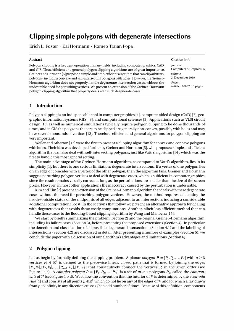
Let us begin by formally defining the clipping problem. A planar polygon P = [P1, P2, . . . , Pn ] with n ≥ 3vertices Pi ∈ R2 is defined as the piecewise linear, closed path that is formed by joining the edges[P1, P2], [P2, P3], . . . , [Pn−1, Pn ], [Pn , P1] that consecutively connect the vertices Pi in the given order (seeFigure 1 a,c). A complex polygon P = {P1, P2, . . . , Pm} is a set of m ≥ 1 polygons P j , called the compon-ents of P (see Figure 1 b,d). We follow the convention that the interior of P is determined by the even-oddrule [4] and consists of all points p ∈R2 which do not lie on any of the edges of P and for which a ray drawnfrom p to infinity in any direction crosses P an odd number of times. Because of this definition, components

1

(a)

P1

P2

Pn

Pi

P

(b)

P

P2

P1

P3

(c) (d)

Figure 1: Examples of a single simple polygon (a), a simple complex polygon with three components and one hole (b),a single self-intersecting polygon (c), and a complex self-intersecting polygon with three components (d), with theirinteriors shaded.

(a) (b) (c)

RP Q

Figure 2: Example of polygon clipping: the intersection of a simple polygon P with three components and one hole (a)and a self-intersecting polygon Q with one component (b) gives a result polygon R with two components, one of themsimple, the other self-intersecting (c).

that are inside other components are commonly referred to as holes (see Figure 1 b). For the sake of brevity,we consider single polygons as complex polygons with one component and refer to complex polygons simplyas polygons. A polygon is called simple if it does not cross itself, that is, its edges intersect only at commonendpoints, which in turn is equivalent to the property that its half-open edges do not intersect at all. Eachcomponent of a simple polygon is thus topologically equivalent to a circle (see Figure 1 a,b).

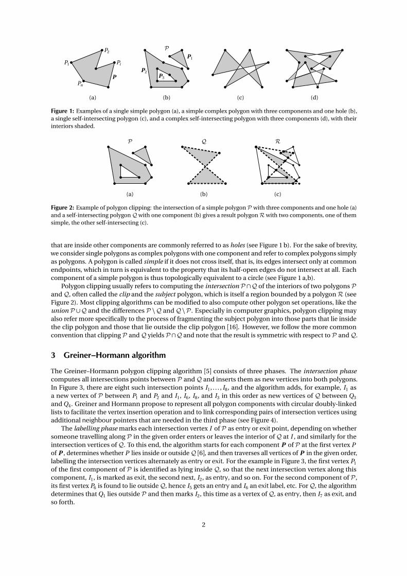
Polygon clipping usually refers to computing the intersection P ∩Q of the interiors of two polygons Pand Q, often called the clip and the subject polygon, which is itself a region bounded by a polygon R (seeFigure 2). Most clipping algorithms can be modified to also compute other polygon set operations, like theunion P ∪Q and the differences P \Q and Q \P . Especially in computer graphics, polygon clipping mayalso refer more specifically to the process of fragmenting the subject polygon into those parts that lie insidethe clip polygon and those that lie outside the clip polygon [16]. However, we follow the more commonconvention that clipping P and Q yields P ∩Q and note that the result is symmetric with respect to P and Q.

3 Greiner–Hormann algorithm

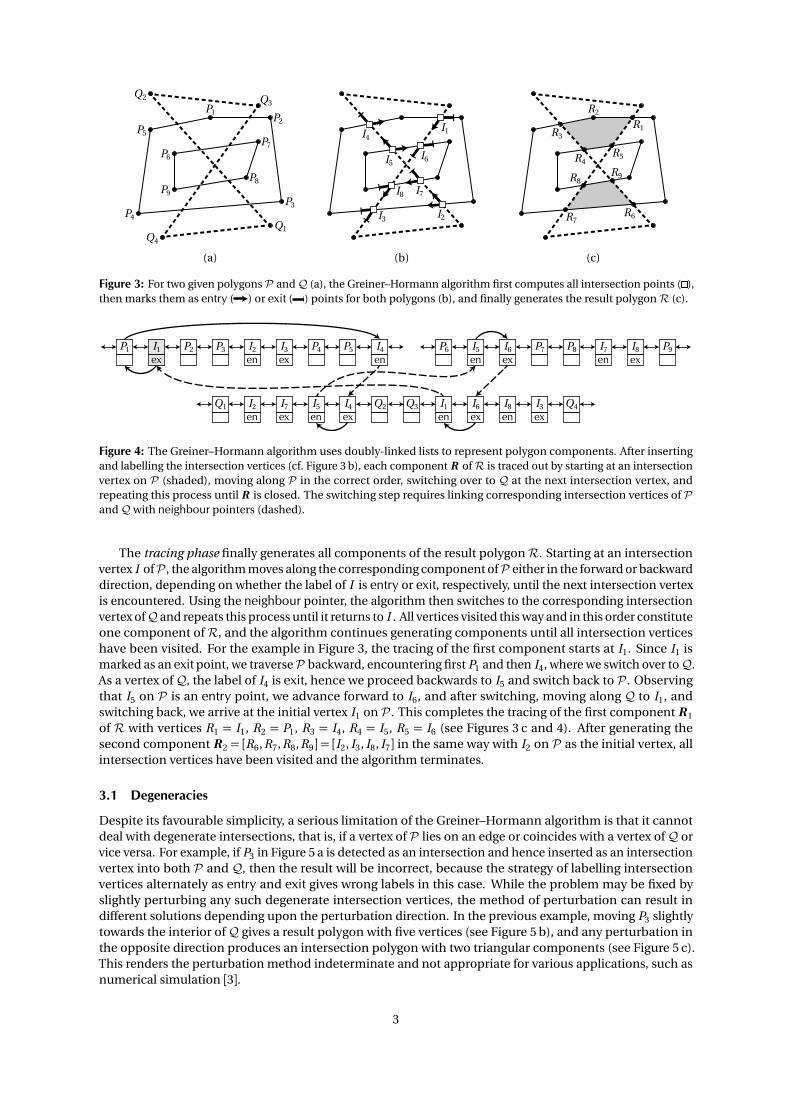
The Greiner–Hormann polygon clipping algorithm [5] consists of three phases. The intersection phasecomputes all intersections points between P and Q and inserts them as new vertices into both polygons.In Figure 3, there are eight such intersection points I1, . . . , I8, and the algorithm adds, for example, I1 asa new vertex of P between P1 and P2 and I1, I6, I8, and I3 in this order as new vertices of Q between Q3

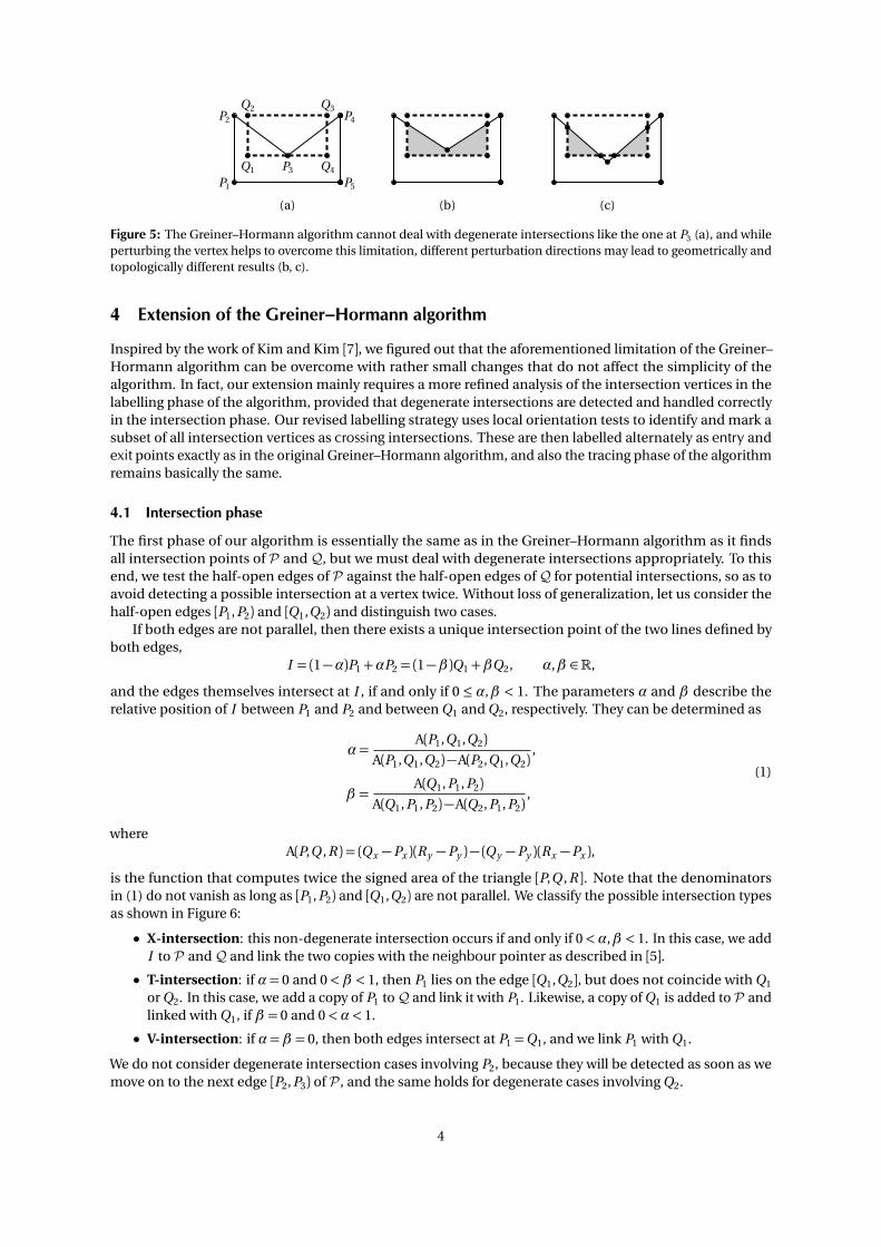
and Q4. Greiner and Hormann propose to represent all polygon components with circular doubly-linkedlists to facilitate the vertex insertion operation and to link corresponding pairs of intersection vertices usingadditional neighbour pointers that are needed in the third phase (see Figure 4).

The labelling phase marks each intersection vertex I of P as entry or exit point, depending on whethersomeone travelling along P in the given order enters or leaves the interior of Q at I , and similarly for theintersection vertices of Q. To this end, the algorithm starts for each component P of P at the first vertex Pof P , determines whether P lies inside or outside Q [6], and then traverses all vertices of P in the given order,labelling the intersection vertices alternately as entry or exit. For the example in Figure 3, the first vertex P1

of the first component of P is identified as lying inside Q, so that the next intersection vertex along thiscomponent, I1, is marked as exit, the second next, I2, as entry, and so on. For the second component of P ,its first vertex P6 is found to lie outside Q, hence I5 gets an entry and I6 an exit label, etc. For Q, the algorithmdetermines that Q1 lies outside P and then marks I2, this time as a vertex of Q, as entry, then I7 as exit, andso forth.

2

(a) (b) (c)

P4

P5

P1

P3

P2

P6

P7

P8P9

Q2

Q1

Q3

Q4

I4I1

I2I3

I5I6

I7I8

R3

R2

R1

R5R4

R6R7

R8R9

Figure 3: For two given polygons P and Q (a), the Greiner–Hormann algorithm first computes all intersection points ( ),then marks them as entry ( ) or exit ( ) points for both polygons (b), and finally generates the result polygon R (c).

I5 I6P6 P7 P8 P9I7 I8P4 P5P1 P3P2 I4I1 I2 I3

Q2Q1 Q3 Q4I4 I1I2 I3I5 I6I7 I8

enex ex ex ex

ex exen en

enen en

ex exen en

Figure 4: The Greiner–Hormann algorithm uses doubly-linked lists to represent polygon components. After insertingand labelling the intersection vertices (cf. Figure 3 b), each component R of R is traced out by starting at an intersectionvertex on P (shaded), moving along P in the correct order, switching over to Q at the next intersection vertex, andrepeating this process until R is closed. The switching step requires linking corresponding intersection vertices of Pand Q with neighbour pointers (dashed).

The tracing phase finally generates all components of the result polygon R. Starting at an intersectionvertex I ofP , the algorithm moves along the corresponding component ofP either in the forward or backwarddirection, depending on whether the label of I is entry or exit, respectively, until the next intersection vertexis encountered. Using the neighbour pointer, the algorithm then switches to the corresponding intersectionvertex ofQ and repeats this process until it returns to I . All vertices visited this way and in this order constituteone component of R, and the algorithm continues generating components until all intersection verticeshave been visited. For the example in Figure 3, the tracing of the first component starts at I1. Since I1 ismarked as an exit point, we traverse P backward, encountering first P1 and then I4, where we switch over to Q.As a vertex of Q, the label of I4 is exit, hence we proceed backwards to I5 and switch back to P . Observingthat I5 on P is an entry point, we advance forward to I6, and after switching, moving along Q to I1, andswitching back, we arrive at the initial vertex I1 on P . This completes the tracing of the first component R 1

of R with vertices R1 = I1, R2 = P1, R3 = I4, R4 = I5, R5 = I6 (see Figures 3 c and 4). After generating thesecond component R 2 = [R6, R7, R8, R9] = [I2, I3, I8, I7] in the same way with I2 on P as the initial vertex, allintersection vertices have been visited and the algorithm terminates.

3.1 Degeneracies

Despite its favourable simplicity, a serious limitation of the Greiner–Hormann algorithm is that it cannotdeal with degenerate intersections, that is, if a vertex of P lies on an edge or coincides with a vertex of Q orvice versa. For example, if P3 in Figure 5 a is detected as an intersection and hence inserted as an intersectionvertex into both P and Q, then the result will be incorrect, because the strategy of labelling intersectionvertices alternately as entry and exit gives wrong labels in this case. While the problem may be fixed byslightly perturbing any such degenerate intersection vertices, the method of perturbation can result indifferent solutions depending upon the perturbation direction. In the previous example, moving P3 slightlytowards the interior of Q gives a result polygon with five vertices (see Figure 5 b), and any perturbation inthe opposite direction produces an intersection polygon with two triangular components (see Figure 5 c).This renders the perturbation method indeterminate and not appropriate for various applications, such asnumerical simulation [3].

3

P2

P1

P3

P4

P5

Q1 Q4

Q2 Q3

(a) (b) (c)

Figure 5: The Greiner–Hormann algorithm cannot deal with degenerate intersections like the one at P3 (a), and whileperturbing the vertex helps to overcome this limitation, different perturbation directions may lead to geometrically andtopologically different results (b, c).

4 Extension of the Greiner–Hormann algorithm

Inspired by the work of Kim and Kim [7], we figured out that the aforementioned limitation of the Greiner–Hormann algorithm can be overcome with rather small changes that do not affect the simplicity of thealgorithm. In fact, our extension mainly requires a more refined analysis of the intersection vertices in thelabelling phase of the algorithm, provided that degenerate intersections are detected and handled correctlyin the intersection phase. Our revised labelling strategy uses local orientation tests to identify and mark asubset of all intersection vertices as crossing intersections. These are then labelled alternately as entry andexit points exactly as in the original Greiner–Hormann algorithm, and also the tracing phase of the algorithmremains basically the same.

4.1 Intersection phase

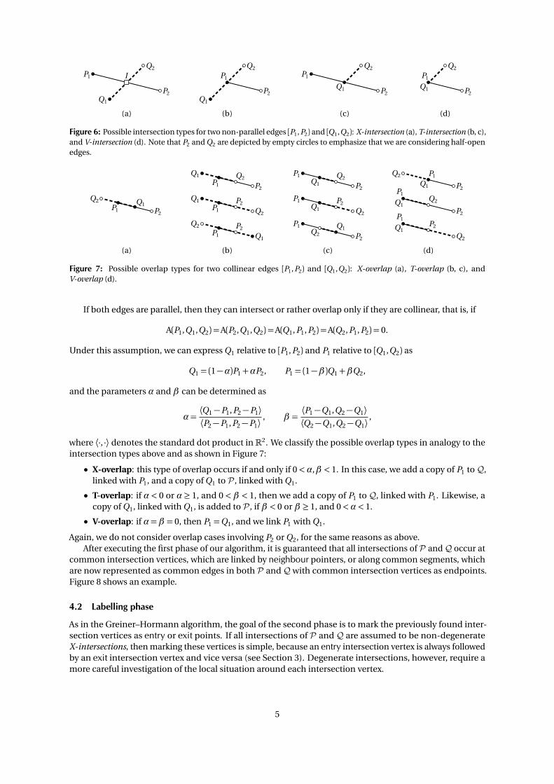
The first phase of our algorithm is essentially the same as in the Greiner–Hormann algorithm as it findsall intersection points of P and Q, but we must deal with degenerate intersections appropriately. To thisend, we test the half-open edges of P against the half-open edges of Q for potential intersections, so as toavoid detecting a possible intersection at a vertex twice. Without loss of generalization, let us consider thehalf-open edges [P1, P2) and [Q1,Q2) and distinguish two cases.

If both edges are not parallel, then there exists a unique intersection point of the two lines defined byboth edges,

I = (1−α)P1+αP2 = (1−β )Q1+βQ2, α,β ∈R,

and the edges themselves intersect at I , if and only if 0 ≤ α,β < 1. The parameters α and β describe therelative position of I between P1 and P2 and between Q1 and Q2, respectively. They can be determined as

α=A(P1,Q1,Q2)

A(P1,Q1,Q2)−A(P2,Q1,Q2),

β =A(Q1, P1, P2)

A(Q1, P1, P2)−A(Q2, P1, P2),

(1)

whereA(P,Q , R ) = (Qx −Px )(Ry −Py )− (Qy −Py )(Rx −Px ),

is the function that computes twice the signed area of the triangle [P,Q , R ]. Note that the denominatorsin (1) do not vanish as long as [P1, P2) and [Q1,Q2) are not parallel. We classify the possible intersection typesas shown in Figure 6:

• X-intersection: this non-degenerate intersection occurs if and only if 0<α,β < 1. In this case, we addI to P and Q and link the two copies with the neighbour pointer as described in [5].

• T-intersection: if α= 0 and 0<β < 1, then P1 lies on the edge [Q1,Q2], but does not coincide with Q1

or Q2. In this case, we add a copy of P1 to Q and link it with P1. Likewise, a copy of Q1 is added to P andlinked with Q1, if β = 0 and 0<α< 1.

• V-intersection: if α=β = 0, then both edges intersect at P1 =Q1, and we link P1 with Q1.

We do not consider degenerate intersection cases involving P2, because they will be detected as soon as wemove on to the next edge [P2, P3) of P , and the same holds for degenerate cases involving Q2.

4

P1

P2

Q2

Q1

P1

P2

Q2

Q1

P1

P2

Q2

Q1 P2

Q2

Q1

P1I

(a) (b) (d)(c)

Figure 6: Possible intersection types for two non-parallel edges [P1, P2) and [Q1,Q2): X-intersection (a), T-intersection (b, c),and V-intersection (d). Note that P2 and Q2 are depicted by empty circles to emphasize that we are considering half-openedges.

(a) (b) (c) (d)

P1

Q2

Q1

P1Q2

Q1

P2

P2

Q2Q1

P1

P1 P2

Q2 Q1 P1

Q1

Q2

P2

P1Q1 Q2

P2

Q2 P1

Q1

P2

P1 P2

Q1 Q2

P2

P1Q1 P2

Q2

Q2

Q1

P1P2

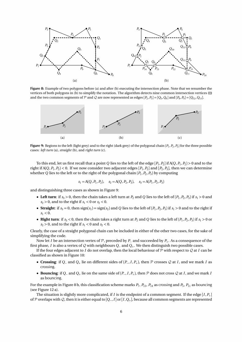
Figure 7: Possible overlap types for two collinear edges [P1, P2) and [Q1,Q2): X-overlap (a), T-overlap (b, c), andV-overlap (d).

If both edges are parallel, then they can intersect or rather overlap only if they are collinear, that is, if

A(P1,Q1,Q2) =A(P2,Q1,Q2) =A(Q1, P1, P2) =A(Q2, P1, P2) = 0.

Under this assumption, we can express Q1 relative to [P1, P2) and P1 relative to [Q1,Q2) as

Q1 = (1−α)P1+αP2, P1 = (1−β )Q1+βQ2,

and the parameters α and β can be determined as

α=⟨Q1−P1, P2−P1⟩⟨P2−P1, P2−P1⟩ , β =

⟨P1−Q1,Q2−Q1⟩⟨Q2−Q1,Q2−Q1⟩ ,

where ⟨·, ·⟩ denotes the standard dot product inR2. We classify the possible overlap types in analogy to theintersection types above and as shown in Figure 7:

• X-overlap: this type of overlap occurs if and only if 0<α,β < 1. In this case, we add a copy of P1 to Q,linked with P1, and a copy of Q1 to P , linked with Q1.

• T-overlap: if α < 0 or α≥ 1, and 0< β < 1, then we add a copy of P1 to Q, linked with P1. Likewise, acopy of Q1, linked with Q1, is added to P , if β < 0 or β ≥ 1, and 0<α< 1.

• V-overlap: if α=β = 0, then P1 =Q1, and we link P1 with Q1.

Again, we do not consider overlap cases involving P2 or Q2, for the same reasons as above.After executing the first phase of our algorithm, it is guaranteed that all intersections of P and Q occur at

common intersection vertices, which are linked by neighbour pointers, or along common segments, whichare now represented as common edges in both P and Q with common intersection vertices as endpoints.Figure 8 shows an example.

4.2 Labelling phase

As in the Greiner–Hormann algorithm, the goal of the second phase is to mark the previously found inter-section vertices as entry or exit points. If all intersections of P and Q are assumed to be non-degenerateX-intersections, then marking these vertices is simple, because an entry intersection vertex is always followedby an exit intersection vertex and vice versa (see Section 3). Degenerate intersections, however, require amore careful investigation of the local situation around each intersection vertex.

5

P1

P2

P3 P5

P4

P6

P7

P8

P9

Q2Q1

Q3

Q4

Q5

Q6

P1

P3

P4 P6

P5

P8

P9

P10

P12

P2

P7

P11P13P14

Q4Q1

Q6

Q8

Q10

Q11

Q2Q3

Q5

Q7 Q9Q12

Q13

(a) (b)

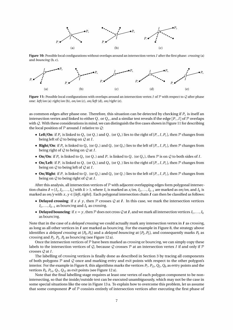
Figure 8: Example of two polygons before (a) and after (b) executing the intersection phase. Note that we renumber thevertices of both polygons in (b) to simplify the notation. The algorithm detects nine common intersection vertices ( )and the two common segments of P and Q are now represented as edges [P2, P3] = [Q5,Q6] and [P8, P9] = [Q12,Q13].

(b) (c)(a)

P1

P3

P2 P1

P3

P2P1

P3

P2

Figure 9: Regions to the left (light grey) and to the right (dark grey) of the polygonal chain (P1, P2, P3) for the three possiblecases: left turn (a), straight (b), and right turn (c).

To this end, let us first recall that a point Q lies to the left of the edge [P1, P2] if A(Q , P1, P2)> 0 and to theright if A(Q , P1, P2) < 0. If we now consider two adjacent edges [P1, P2] and [P2, P3], then we can determinewhether Q lies to the left or to the right of the polygonal chain (P1, P2, P3) by computing

s1 =A(Q , P1, P2), s2 =A(Q , P2, P3), s3 =A(P1, P2, P3)

and distinguishing three cases as shown in Figure 9:

• Left turn: if s3 > 0, then the chain takes a left turn at P2 and Q lies to the left of (P1, P2, P3) if s1 > 0 ands2 > 0, and to the right if s1 < 0 or s2 < 0.

• Straight: if s3 = 0, then sign(s1) = sign(s2) and Q lies to the left of (P1, P2, P3) if s1 > 0 and to the right ifs1 < 0.

• Right turn: if s3 < 0, then the chain takes a right turn at P2 and Q lies to the left of (P1, P2, P3) if s1 > 0 ors2 > 0, and to the right if s1 < 0 and s2 < 0.

Clearly, the case of a straight polygonal chain can be included in either of the other two cases, for the sake ofsimplifying the code.

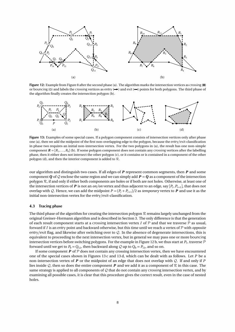
Now let I be an intersection vertex of P , preceded by P− and succeeded by P+. As a consequence of thefirst phase, I is also a vertex of Q with neighbours Q− and Q+. We then distinguish two possible cases.

If the four edges adjacent to I do not overlap, then the local behaviour of P with respect to Q at I can beclassified as shown in Figure 10:

• Crossing: if Q− and Q+ lie on different sides of (P−, I , P+), then P crosses Q at I , and we mark I ascrossing.

• Bouncing: if Q− and Q+ lie on the same side of (P−, I , P+), then P does not cross Q at I , and we mark Ias bouncing.

For the example in Figure 8 b, this classification scheme marks P7, P13, P14 as crossing and P5, P11 as bouncing(see Figure 12 a).

The situation is slightly more complicated, if I is the endpoint of a common segment. If the edge [I , P+]of P overlaps with Q, then it is either equal to [Q−, I ] or [I ,Q+], because all common segments are represented

6

(b) (c)(a)

P−

P+

I P−

P+I

P−

P+

I

Figure 10: Possible local configurations without overlaps around an intersection vertex I after the first phase: crossing (a)and bouncing (b, c).

(a) (b) (c) (e)(d)

P−

P+I

P−

P+

IP−

P+I

P−

P+

IP−

P+I

Figure 11: Possible local configurations with overlaps around an intersection vertex I of P with respect to Q after phaseone: left/on (a) right/on (b), on/on (c), on/left (d), on/right (e).

as common edges after phase one. Therefore, this situation can be detected by checking if P+ is itself anintersection vertex and linked to either Q− or Q+, and a similar test reveals if the edge [P−, I ] of P overlapswithQ. With these considerations in mind, we can distinguish the five cases shown in Figure 11 for describingthe local position of P around I relative to Q:

• Left/On: if P+ is linked to Q+ (or Q−) and Q− (or Q+) lies to the right of (P−, I , P+), then P changes frombeing left of Q to being on Q at I .

• Right/On: if P+ is linked to Q+ (or Q−) and Q− (or Q+) lies to the left of (P−, I , P+), then P changes frombeing right of Q to being on Q at I .

• On/On: if P+ is linked to Q+ (or Q−) and P− is linked to Q− (or Q+), then P is on Q to both sides of I .

• On/Left: if P− is linked to Q− (or Q+) and Q+ (or Q−) lies to the right of (P−, I , P+), then P changes frombeing on Q to being left of Q at I .

• On/Right: if P− is linked to Q− (or Q+) and Q+ (or Q−) lies to the left of (P−, I , P+), then P changes frombeing on Q to being right of Q at I .

After this analysis, all intersection vertices of P with adjacent overlapping edges form polygonal intersec-tion chains I = (I1, I2, . . . , Ik )with k > 1, where I1 is marked as x/on, I2, . . . , Ik−1 are marked as on/on, and Ik ismarked as on/y with x , y ∈ {left, right}. Each polygonal intersection chain I can then be classified as follows:

• Delayed crossing: if x 6= y , then P crosses Q at I . In this case, we mark the intersection verticesI1, . . . , Ik−1 as bouncing and Ik as crossing.

• Delayed bouncing: if x = y , thenP does not crossQ at I , and we mark all intersection vertices I1, . . . , Ik

as bouncing.

Note that in the case of a delayed crossing we could actually mark any intersection vertex in I as crossing,as long as all other vertices in I are marked as bouncing. For the example in Figure 8, the strategy aboveidentifies a delayed crossing at (P8, P9) and a delayed bouncing at (P2, P3), and consequently marks P9 ascrossing and P2, P3, P8 as bouncing (see Figure 12 a).

Once the intersection vertices of P have been marked as crossing or bouncing, we can simply copy theselabels to the intersection vertices of Q, because Q crosses P at an intersection vertex I if and only if Pcrosses Q at I .

The labelling of crossing vertices is finally done as described in Section 3 by tracing all componentsof both polygons P and Q once and marking entry and exit points with respect to the other polygon’sinterior. For the example in Figure 8, this algorithms marks the vertices P7, P13, Q2, Q9 as entry points and thevertices P9, P14, Q7, Q12 as exit points (see Figure 12 a).

Note that the final labelling stage requires at least one vertex of each polygon component to be non-intersecting, so that the inside/outside test can be executed unambiguously, which may not be the case insome special situations like the one in Figure 13 a. To explain how to overcome this problem, let us assumethat some component P of P consists entirely of intersection vertices after executing the first phase of

7

P3

P5

P8

P9

P2

P7

P11P13P14

Q6

Q11

Q2Q3

Q5

Q7 Q9Q12

Q13

R1

R2

R3

R4

R5

R6R7

R8

R9

R10R11

(a) (b)

Figure 12: Example from Figure 8 after the second phase (a). The algorithm marks the intersection vertices as crossing ( )or bouncing ( ) and labels the crossing vertices as entry ( ) and exit ( ) points for both polygons. The third phase ofthe algorithm finally creates the intersection polygon (b).

P1 P2

P3P5 P4

P6

P

Q2

Q1

Q3

Q4

Q5 Q6

Q

R5

R4

R7

R2

R1

R9

R6

R3

R8

(a) (b) (d)(c)

Figure 13: Examples of some special cases. If a polygon component consists of intersection vertices only after phaseone (a), then we add the midpoint of the first non-overlapping edge to the polygon, because the entry/exit-classificationin phase two requires an initial non-intersection vertex. For the two polygons in (a), the result has one non-simplecomponent R = [R1, . . . , R9] (b). If some polygon component does not contain any crossing vertices after the labellingphase, then it either does not intersect the other polygon (c), or it contains or is contained in a component of the otherpolygon (d), and then the interior component is added to R.

our algorithm and distinguish two cases. If all edges of P represent common segments, then P and somecomponent Q of Q enclose the same region and we can simply add P =Q as a component of the intersectionpolygon R, if and only if either both components are holes or if both are not holes. Otherwise, at least one ofthe intersection vertices of P is not an on/on vertex and thus adjacent to an edge, say [Pi , Pi+1], that does notoverlap with Q. Hence, we can add the midpoint P = (Pi +Pi+1)/2 as temporary vertex to P and use it as theinitial non-intersection vertex for the entry/exit-classification.

4.3 Tracing phase

The third phase of the algorithm for creating the intersection polygon R remains largely unchanged from theoriginal Greiner–Hormann algorithm and is described in Section 3. The only difference is that the generationof each result component starts at a crossing intersection vertex I of P and that we traverse P as usual,forward if I is an entry point and backward otherwise, but this time until we reach a vertex of P with oppositeentry/exit flag, and likewise after switching over to Q. In the absence of degenerate intersections, this isequivalent to proceeding to the next intersection vertex, but in general we may pass one or more bouncingintersection vertices before switching polygons. For the example in Figure 12 b, we thus start at P7, traverse Pforward until we get to P9 =Q12, then backward along Q up to Q9 = P13, and so on.

If some component P of P does not contain any crossing intersection vertex, then we have encounteredone of the special cases shown in Figures 13 c and 13 d, which can be dealt with as follows. Let P be anon-intersection vertex of P or the midpoint of an edge that does not overlap with Q. If and only if Plies inside Q, then so does the entire component P and we add it as a component of R in this case. Thesame strategy is applied to all components of Q that do not contain any crossing intersection vertex, and byexamining all possible cases, it is clear that this procedure gives the correct result, even in the case of nestedholes.

8

(a) (c)(b) (d)

P8

P9

Q7

P2

Q6

Q9Q1

Q8

P1

Q5P6

P7

P3Q2

R5

R1

R3

R7

R2R6

R4

PQ

P ′Q ′

R7

R1

R5

R3

R2R4

R6

Q3 P4

Q4P5

P−

P+

Q−

Q+

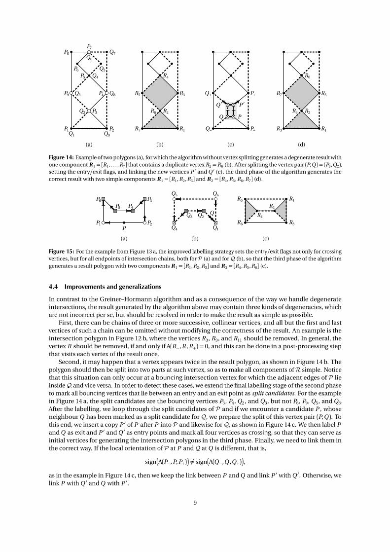
Figure 14: Example of two polygons (a), for which the algorithm without vertex splitting generates a degenerate result withone component R 1 = [R1, . . . , R7] that contains a duplicate vertex R2 =R6 (b). After splitting the vertex pair (P,Q ) = (P3,Q2),setting the entry/exit flags, and linking the new vertices P ′ and Q ′ (c), the third phase of the algorithm generates thecorrect result with two simple components R 1 = [R1, R2, R3] and R 2 = [R4, R5, R6, R7] (d).

(a) (b) (c)

P1 P2

P3

P5 P4

P6

P

Q2

Q1

Q3

Q4

Q5 Q6

Q

R1

R2

R5

R6

R4

R3

Figure 15: For the example from Figure 13 a, the improved labelling strategy sets the entry/exit flags not only for crossingvertices, but for all endpoints of intersection chains, both for P (a) and for Q (b), so that the third phase of the algorithmgenerates a result polygon with two components R 1 = [R1, R2, R3] and R 2 = [R4, R5, R6] (c).

4.4 Improvements and generalizations

In contrast to the Greiner–Hormann algorithm and as a consequence of the way we handle degenerateintersections, the result generated by the algorithm above may contain three kinds of degeneracies, whichare not incorrect per se, but should be resolved in order to make the result as simple as possible.

First, there can be chains of three or more successive, collinear vertices, and all but the first and lastvertices of such a chain can be omitted without modifying the correctness of the result. An example is theintersection polygon in Figure 12 b, where the vertices R3, R9, and R11 should be removed. In general, thevertex R should be removed, if and only if A(R−, R , R+) = 0, and this can be done in a post-processing stepthat visits each vertex of the result once.

Second, it may happen that a vertex appears twice in the result polygon, as shown in Figure 14 b. Thepolygon should then be split into two parts at such vertex, so as to make all components of R simple. Noticethat this situation can only occur at a bouncing intersection vertex for which the adjacent edges of P lieinside Q and vice versa. In order to detect these cases, we extend the final labelling stage of the second phaseto mark all bouncing vertices that lie between an entry and an exit point as split candidates. For the examplein Figure 14 a, the split candidates are the bouncing vertices P3, P4, Q2, and Q3, but not P6, P9, Q5, and Q8.After the labelling, we loop through the split candidates of P and if we encounter a candidate P , whoseneighbour Q has been marked as a split candidate for Q, we prepare the split of this vertex pair (P,Q ). Tothis end, we insert a copy P ′ of P after P into P and likewise for Q, as shown in Figure 14 c. We then label Pand Q as exit and P ′ and Q ′ as entry points and mark all four vertices as crossing, so that they can serve asinitial vertices for generating the intersection polygons in the third phase. Finally, we need to link them inthe correct way. If the local orientation of P at P and Q at Q is different, that is,

sign�

A(P−, P, P+)� 6= sign�

A(Q−,Q ,Q+)�

,

as in the example in Figure 14 c, then we keep the link between P and Q and link P ′ with Q ′. Otherwise, welink P with Q ′ and Q with P ′.

9

(a) (b) (c)

P1 P2Q2

Q1

Q3

Q4

P4 P3

Q6

Q5

R3 R2

R5R41

R2 R1

R4R3

R1

R6

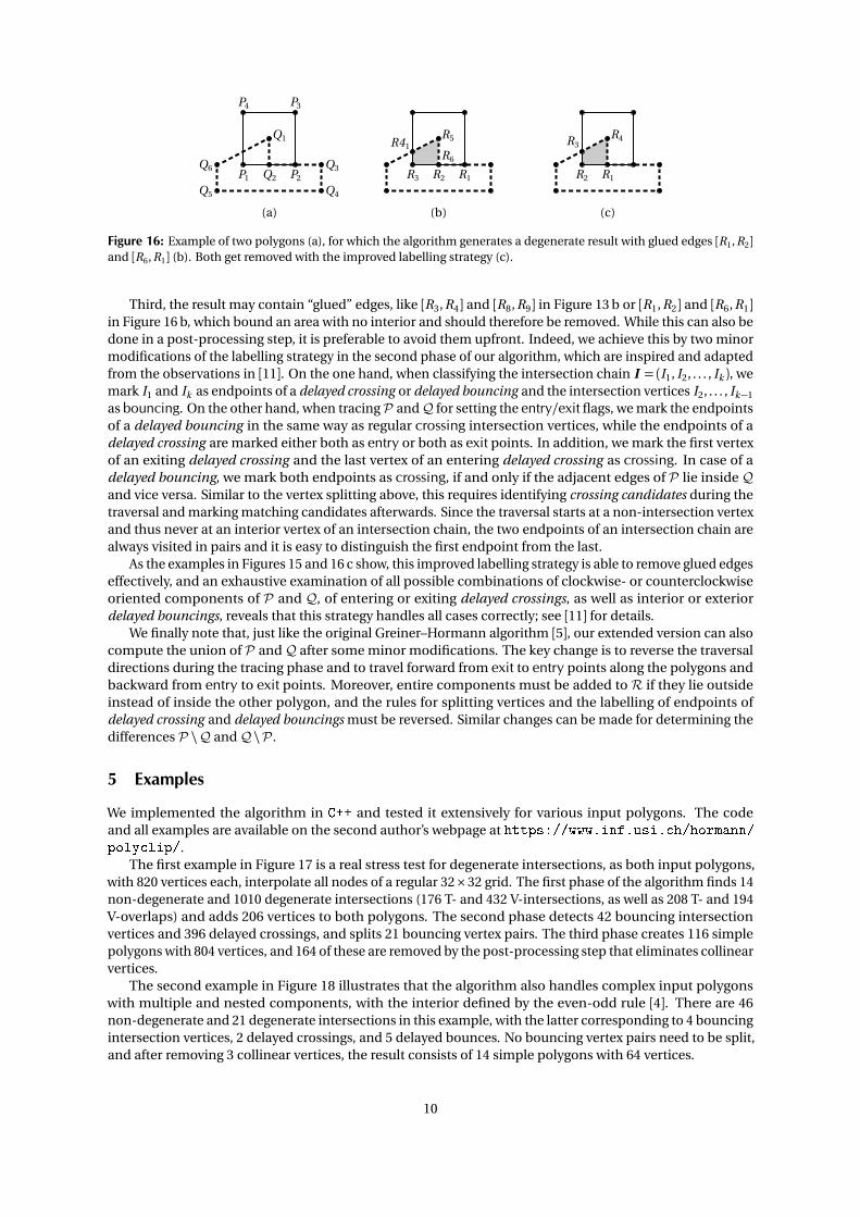
Figure 16: Example of two polygons (a), for which the algorithm generates a degenerate result with glued edges [R1, R2]and [R6, R1] (b). Both get removed with the improved labelling strategy (c).

Third, the result may contain “glued” edges, like [R3, R4] and [R8, R9] in Figure 13 b or [R1, R2] and [R6, R1]in Figure 16 b, which bound an area with no interior and should therefore be removed. While this can also bedone in a post-processing step, it is preferable to avoid them upfront. Indeed, we achieve this by two minormodifications of the labelling strategy in the second phase of our algorithm, which are inspired and adaptedfrom the observations in [11]. On the one hand, when classifying the intersection chain I = (I1, I2, . . . , Ik ), wemark I1 and Ik as endpoints of a delayed crossing or delayed bouncing and the intersection vertices I2, . . . , Ik−1

as bouncing. On the other hand, when tracing P and Q for setting the entry/exit flags, we mark the endpointsof a delayed bouncing in the same way as regular crossing intersection vertices, while the endpoints of adelayed crossing are marked either both as entry or both as exit points. In addition, we mark the first vertexof an exiting delayed crossing and the last vertex of an entering delayed crossing as crossing. In case of adelayed bouncing, we mark both endpoints as crossing, if and only if the adjacent edges of P lie inside Qand vice versa. Similar to the vertex splitting above, this requires identifying crossing candidates during thetraversal and marking matching candidates afterwards. Since the traversal starts at a non-intersection vertexand thus never at an interior vertex of an intersection chain, the two endpoints of an intersection chain arealways visited in pairs and it is easy to distinguish the first endpoint from the last.

As the examples in Figures 15 and 16 c show, this improved labelling strategy is able to remove glued edgeseffectively, and an exhaustive examination of all possible combinations of clockwise- or counterclockwiseoriented components of P and Q, of entering or exiting delayed crossings, as well as interior or exteriordelayed bouncings, reveals that this strategy handles all cases correctly; see [11] for details.

We finally note that, just like the original Greiner–Hormann algorithm [5], our extended version can alsocompute the union of P and Q after some minor modifications. The key change is to reverse the traversaldirections during the tracing phase and to travel forward from exit to entry points along the polygons andbackward from entry to exit points. Moreover, entire components must be added to R if they lie outsideinstead of inside the other polygon, and the rules for splitting vertices and the labelling of endpoints ofdelayed crossing and delayed bouncings must be reversed. Similar changes can be made for determining thedifferences P \Q and Q \P .

5 Examples

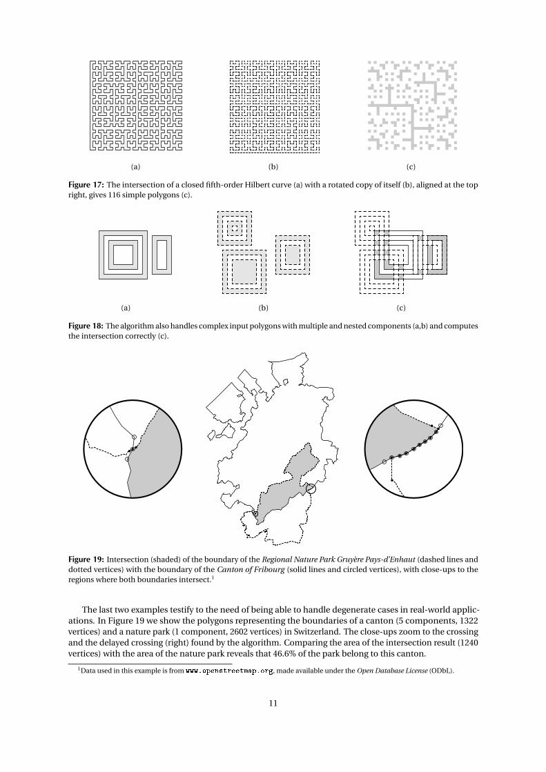
We implemented the algorithm in C++ and tested it extensively for various input polygons. The codeand all examples are available on the second author’s webpage at https://www.inf.usi.ch/hormann/polyclip/.

The first example in Figure 17 is a real stress test for degenerate intersections, as both input polygons,with 820 vertices each, interpolate all nodes of a regular 32×32 grid. The first phase of the algorithm finds 14non-degenerate and 1010 degenerate intersections (176 T- and 432 V-intersections, as well as 208 T- and 194V-overlaps) and adds 206 vertices to both polygons. The second phase detects 42 bouncing intersectionvertices and 396 delayed crossings, and splits 21 bouncing vertex pairs. The third phase creates 116 simplepolygons with 804 vertices, and 164 of these are removed by the post-processing step that eliminates collinearvertices.

The second example in Figure 18 illustrates that the algorithm also handles complex input polygonswith multiple and nested components, with the interior defined by the even-odd rule [4]. There are 46non-degenerate and 21 degenerate intersections in this example, with the latter corresponding to 4 bouncingintersection vertices, 2 delayed crossings, and 5 delayed bounces. No bouncing vertex pairs need to be split,and after removing 3 collinear vertices, the result consists of 14 simple polygons with 64 vertices.

10

(a) (b) (c)

Figure 17: The intersection of a closed fifth-order Hilbert curve (a) with a rotated copy of itself (b), aligned at the topright, gives 116 simple polygons (c).

(a) (b) (c)

Figure 18: The algorithm also handles complex input polygons with multiple and nested components (a,b) and computesthe intersection correctly (c).

Figure 19: Intersection (shaded) of the boundary of the Regional Nature Park Gruyère Pays-d’Enhaut (dashed lines anddotted vertices) with the boundary of the Canton of Fribourg (solid lines and circled vertices), with close-ups to theregions where both boundaries intersect.1

The last two examples testify to the need of being able to handle degenerate cases in real-world applic-ations. In Figure 19 we show the polygons representing the boundaries of a canton (5 components, 1322vertices) and a nature park (1 component, 2602 vertices) in Switzerland. The close-ups zoom to the crossingand the delayed crossing (right) found by the algorithm. Comparing the area of the intersection result (1240vertices) with the area of the nature park reveals that 46.6% of the park belong to this canton.

1Data used in this example is from www.openstreetmap.org, made available under the Open Database License (ODbL).

11

(a) (b) (c) (d)

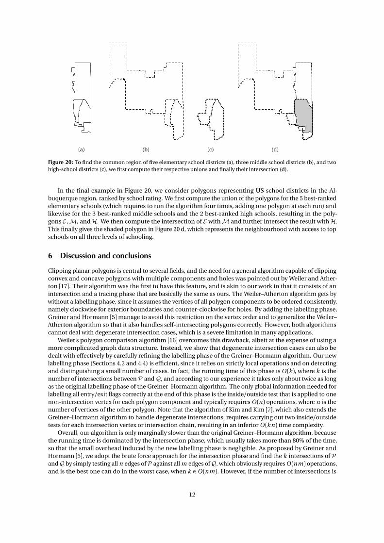
Figure 20: To find the common region of five elementary school districts (a), three middle school districts (b), and twohigh-school districts (c), we first compute their respective unions and finally their intersection (d).

In the final example in Figure 20, we consider polygons representing US school districts in the Al-buquerque region, ranked by school rating. We first compute the union of the polygons for the 5 best-rankedelementary schools (which requires to run the algorithm four times, adding one polygon at each run) andlikewise for the 3 best-ranked middle schools and the 2 best-ranked high schools, resulting in the poly-gons E , M, and H. We then compute the intersection of E with M and further intersect the result with H.This finally gives the shaded polygon in Figure 20 d, which represents the neighbourhood with access to topschools on all three levels of schooling.

6 Discussion and conclusions

Clipping planar polygons is central to several fields, and the need for a general algorithm capable of clippingconvex and concave polygons with multiple components and holes was pointed out by Weiler and Ather-ton [17]. Their algorithm was the first to have this feature, and is akin to our work in that it consists of anintersection and a tracing phase that are basically the same as ours. The Weiler–Atherton algorithm gets bywithout a labelling phase, since it assumes the vertices of all polygon components to be ordered consistently,namely clockwise for exterior boundaries and counter-clockwise for holes. By adding the labelling phase,Greiner and Hormann [5]manage to avoid this restriction on the vertex order and to generalize the Weiler–Atherton algorithm so that it also handles self-intersecting polygons correctly. However, both algorithmscannot deal with degenerate intersection cases, which is a severe limitation in many applications.

Weiler’s polygon comparison algorithm [16] overcomes this drawback, albeit at the expense of using amore complicated graph data structure. Instead, we show that degenerate intersection cases can also bedealt with effectively by carefully refining the labelling phase of the Greiner–Hormann algorithm. Our newlabelling phase (Sections 4.2 and 4.4) is efficient, since it relies on strictly local operations and on detectingand distinguishing a small number of cases. In fact, the running time of this phase is O (k ), where k is thenumber of intersections between P and Q, and according to our experience it takes only about twice as longas the original labelling phase of the Greiner–Hormann algorithm. The only global information needed forlabelling all entry/exit flags correctly at the end of this phase is the inside/outside test that is applied to onenon-intersection vertex for each polygon component and typically requires O (n ) operations, where n is thenumber of vertices of the other polygon. Note that the algorithm of Kim and Kim [7], which also extends theGreiner–Hormann algorithm to handle degenerate intersections, requires carrying out two inside/outsidetests for each intersection vertex or intersection chain, resulting in an inferior O (k n ) time complexity.

Overall, our algorithm is only marginally slower than the original Greiner–Hormann algorithm, becausethe running time is dominated by the intersection phase, which usually takes more than 80% of the time,so that the small overhead induced by the new labelling phase is negligible. As proposed by Greiner andHormann [5], we adopt the brute force approach for the intersection phase and find the k intersections of Pand Q by simply testing all n edges of P against all m edges of Q, which obviously requires O (nm ) operations,and is the best one can do in the worst case, when k ∈O (nm ). However, if the number of intersections is

12

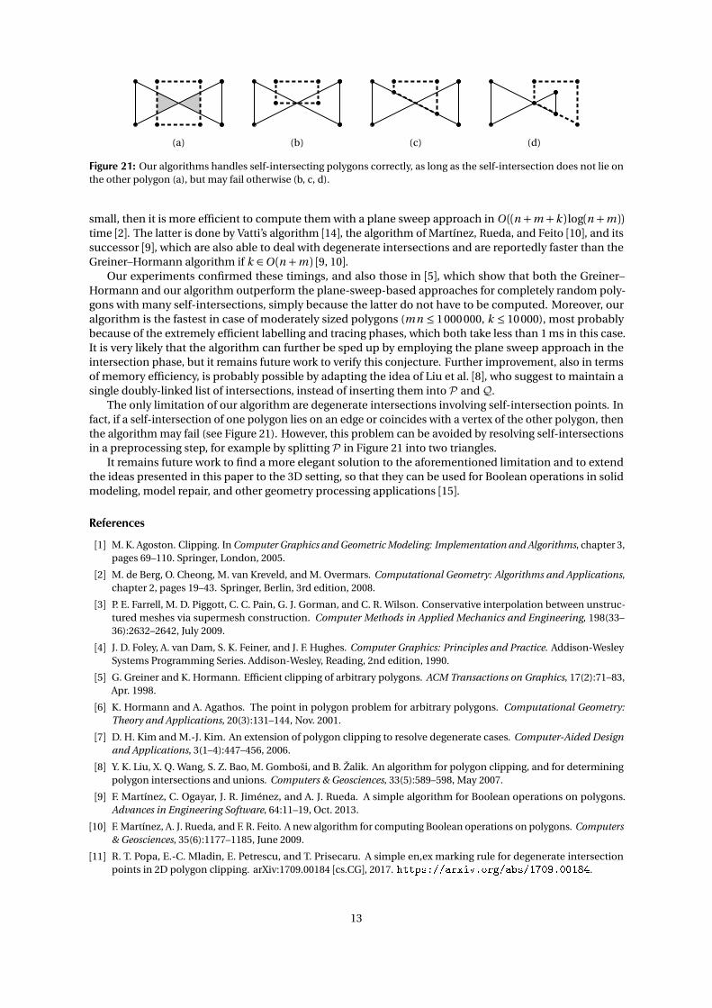
(a) (b) (c) (d)

Figure 21: Our algorithms handles self-intersecting polygons correctly, as long as the self-intersection does not lie onthe other polygon (a), but may fail otherwise (b, c, d).

small, then it is more efficient to compute them with a plane sweep approach in O ((n +m +k ) log(n +m ))time [2]. The latter is done by Vatti’s algorithm [14], the algorithm of Martínez, Rueda, and Feito [10], and itssuccessor [9], which are also able to deal with degenerate intersections and are reportedly faster than theGreiner–Hormann algorithm if k ∈O (n +m ) [9, 10].

Our experiments confirmed these timings, and also those in [5], which show that both the Greiner–Hormann and our algorithm outperform the plane-sweep-based approaches for completely random poly-gons with many self-intersections, simply because the latter do not have to be computed. Moreover, ouralgorithm is the fastest in case of moderately sized polygons (mn ≤ 1000000, k ≤ 10000), most probablybecause of the extremely efficient labelling and tracing phases, which both take less than 1 ms in this case.It is very likely that the algorithm can further be sped up by employing the plane sweep approach in theintersection phase, but it remains future work to verify this conjecture. Further improvement, also in termsof memory efficiency, is probably possible by adapting the idea of Liu et al. [8], who suggest to maintain asingle doubly-linked list of intersections, instead of inserting them into P and Q.

The only limitation of our algorithm are degenerate intersections involving self-intersection points. Infact, if a self-intersection of one polygon lies on an edge or coincides with a vertex of the other polygon, thenthe algorithm may fail (see Figure 21). However, this problem can be avoided by resolving self-intersectionsin a preprocessing step, for example by splitting P in Figure 21 into two triangles.

It remains future work to find a more elegant solution to the aforementioned limitation and to extendthe ideas presented in this paper to the 3D setting, so that they can be used for Boolean operations in solidmodeling, model repair, and other geometry processing applications [15].

References

[1] M. K. Agoston. Clipping. In Computer Graphics and Geometric Modeling: Implementation and Algorithms, chapter 3,pages 69–110. Springer, London, 2005.

[2] M. de Berg, O. Cheong, M. van Kreveld, and M. Overmars. Computational Geometry: Algorithms and Applications,chapter 2, pages 19–43. Springer, Berlin, 3rd edition, 2008.

[3] P. E. Farrell, M. D. Piggott, C. C. Pain, G. J. Gorman, and C. R. Wilson. Conservative interpolation between unstruc-tured meshes via supermesh construction. Computer Methods in Applied Mechanics and Engineering, 198(33–36):2632–2642, July 2009.

[4] J. D. Foley, A. van Dam, S. K. Feiner, and J. F. Hughes. Computer Graphics: Principles and Practice. Addison-WesleySystems Programming Series. Addison-Wesley, Reading, 2nd edition, 1990.

[5] G. Greiner and K. Hormann. Efficient clipping of arbitrary polygons. ACM Transactions on Graphics, 17(2):71–83,Apr. 1998.

[6] K. Hormann and A. Agathos. The point in polygon problem for arbitrary polygons. Computational Geometry:Theory and Applications, 20(3):131–144, Nov. 2001.

[7] D. H. Kim and M.-J. Kim. An extension of polygon clipping to resolve degenerate cases. Computer-Aided Designand Applications, 3(1–4):447–456, 2006.

[8] Y. K. Liu, X. Q. Wang, S. Z. Bao, M. Gomboši, and B. Žalik. An algorithm for polygon clipping, and for determiningpolygon intersections and unions. Computers & Geosciences, 33(5):589–598, May 2007.

[9] F. Martínez, C. Ogayar, J. R. Jiménez, and A. J. Rueda. A simple algorithm for Boolean operations on polygons.Advances in Engineering Software, 64:11–19, Oct. 2013.

[10] F. Martínez, A. J. Rueda, and F. R. Feito. A new algorithm for computing Boolean operations on polygons. Computers& Geosciences, 35(6):1177–1185, June 2009.

[11] R. T. Popa, E.-C. Mladin, E. Petrescu, and T. Prisecaru. A simple en,ex marking rule for degenerate intersectionpoints in 2D polygon clipping. arXiv:1709.00184 [cs.CG], 2017. https://arxiv.org/abs/1709.00184.

13

[12] A. Schettino. Polygon intersections in spherical topology: Applications to plate tectonics. Computers & Geosciences,25(1):61–69, Feb. 1999.

[13] L. J. Simonson. Industrial strength polygon clipping: A novel algorithm with applications in VLSI CAD. Computer-Aided Design, 42(12):1189–1196, Dec. 2010.

[14] B. R. Vatti. A generic solution to polygon clipping. Communications of the ACM, 35(7):56–63, July 1992.

[15] C. C. L. Wang and D. Manocha. Efficient boundary extraction of BSP solids based on clipping operations. IEEETransactions on Visualization and Computer Graphics, 19(1):16–29, Jan. 2013.

[16] K. Weiler. Polygon comparison using a graph representation. Computer Graphics, 14(3):10–18, July 1980. Proceedingsof SIGGRAPH.

[17] K. Weiler and P. Atherton. Hidden surface removal using polygon area sorting. Computer Graphics, 11(2):214–222,July 1977. Proceedings of SIGGRAPH.

14