Embed Size (px)
Citation preview

Mathematical Society of the Republic of Moldova
Vladimir Andrunachievici Institute of
Mathematics and Computer Science
Tiraspol State University
Information Society Development Institute
Proceedings IMCS-55
The Fifth Conference
of Mathematical Society
of the Republic of Moldova
dedicated to the 55th anniversary
of the foundation of Vladimir Andrunachievici Institute
of Mathematics and Computer Science
September 28 – October 1, 2019
Chisinau, Republic of Moldova, 2019

Copyright c© Vladimir Andrunachievici Institute of Mathematicsand Computer Science, 2019.All rights reserved.
VLADIMIR ANDRUNACHIEVICI INSTITUTE OF MATHE-MATICS AND COMPUTER SCIENCE5, Academiei street, Chisinau, Republic of Moldova, MD 2028Tel: (373 22) 72-59-82, Fax: (373 22) 73-80-27,E-mail: [email protected] address: http://www.math.md
Editors: Mitrofan Choban, Inga Titchiev.
Authors are fully responsible for the content of their papers.
This issue is supported by grant 19.00059.50.03A/MS, “IMCS-55 – The Fifth
Conference of the Mathematical Society of Moldova – international confer-
ence dedicated to the 55th anniversary of the foundation of the Vladimir An-
drunachievici Institute of Mathematics and Computer Science”.
CZU [51+004](478)(082)
C 65
Descrierea CIP a Camerei Naţionale a Cărţii
"Conference of Mathematical Society of the Republic of Moldova", (5 ; 2019 ;
Chişinău). The Fifth Conference of Mathematical Society of the Republic of
Moldova : dedicated to the 55th anniversary of the foundation of Vladimir
Andrunachievici Institute of Mathematics and Computer Science, September 28 –
October 1, 2019 Chisinau, Republic of Moldova : Proceedings IMCS-55 / ed.:
Mitrofan Choban, Inga Titchiev. – Chişinău : Vladimir Andrunachievici Institute
of Mathematics and Computer Science, 2019 (Tipogr. "Valinex"). – 346 p. : fig.,
tab.
Antetit.: Mathematical Vladimir Andrunachievici Inst. of Mathematics and
Computer Science Soc. of the Rep. of Moldova, , Tiraspol State Univ. [et al.]. –
Referinţe bibliogr. la sfârşitul art. – 150 ex.
ISBN 978-9975-68-378-4.
[51+004](478)(082)
ISBN 978-9975-68-378-4

Proceedings of the Fifth Conference of Mathematical Society of Moldova
IMCS-55, September 28 - October 1, 2019, Chisinau, Republic of Moldova
Preface
Vladimir Andrunachievici Institute of Mathematics and ComputerScience (IMCS), in this spring celebrates its 55th anniversary from thefoundation. With all certainty we can say that IMCS is a centre ofexcellence for advance research in the domains of pure mathematics,the applied one and computer science.
Founded by the illustrious mathematician Vladimir Andrunachievici,it is an organization with a valuable human potential and with re-markable results in all the mentioned domains. Currently the famousscientific schools in the theory of algebraic rings (founded by acad.V. Andrunachievici), in the qualitative theory of differential equations(founded by acad. C. Sibirschi), in the theory of quasigroups (foundedby Professor V. Belousov), in functional analysis (founded by cor.m. IGorhberg) and in mathematical logic (founded by Dr. A. Kuznetov)continue their successful work and development. More than 30 doctorsin habilitations and 400 PhDs were trained in the Institute.
During these 55 years over 3500 scientific papers and about 155monographs have been published. The Institute publishes the journal“Buletinul Academiei de Stiinte a Republicii Moldova. Matematica”(from 1989 to this day 90 volumes were out), also the journal “Com-puter Science Journal of Moldova” (from 1993 to this day 80 volumeswere out). Other journal in collaboration with colleagues from Poland,“Quasigroups and related systems”, has published 27 volumes.
In the last 25 years the Institute took part in executing more than60 projects with partners from advanced research centres in differentcountries of Europe, Asia, America.
The Fifth Conference of the Mathematical Society of
Moldova is the international conference dedicated to this anniversary
c©2019 by M.Choban, I. Titchiev
3

Mitrofan Choban, Inga Titchiev
and is a continuation of the tradition of reviewing new achievements inmathematics, informatics and information technology and informationexchange with colleagues from major research centers across borders.
The organizers of the IMCS-55 edition are: Mathematical Soci-ety of the Republic of Moldova, Vladimir Andrunachievici Institute ofMathematics and Computer Science in cooperation with Tiraspol StateUniversity and Information Society Development Institute.
During the IMCS-55, the solutions for the most current problemsthat appear in various fields of mathematics and computer science aswell as the socio-economic aspect of modern society are also addressed.The conference considers discussions between the research groups ofuniversities, research institutes and the commercial IT field. In thisregard, it is planned to establish scientific priorities for applying thesolutions found by researchers to specific problems in society, nationaleconomy and abroad as well.
The volume includes 77 papers, covering topics in major areas ofmathematics and informatics. It is divided in 3 chapters: Pure Math-ematics, Applied Mathematics and Computer Science.
We express our sincere thanks to all people who contributed to thesuccess of this event, especially from the Scientific Committee, whospent time carefully reviewing all the proposals submitted to IMCS-55 to insure a qualitative improvement of the papers, and from theOrganizing Committee which ensured its high level.
Mitrofan Choban
Inga Titchiev
4

Proceedings of the Fifth Conference of Mathematical Society of Moldova
IMCS-55, September 28 - October 1, 2019, Chisinau, Republic of Moldova
Section 1
Pure Mathematics
5

Proceedings of the 5th Conference of Mathematical Society of Moldova
6

IMCS-55
A computer-friendly alternative to
Morse-Novikov theory
Dan Burghelea
Abstract
Classical Morse-Novikov theory relates the “dynamics ele-ments” of a flow provided by a “Morse-Smale vector field” X
equipped with a Lyapunov closed differential one form (=action)on a closed manifold M to the algebraic topology of the under-lying manifold M .
The Alternative to Morse Novikov (AMN) theory I proposeextends considerably the class of spaces and flows the theoryapplies, providing the same relations. The new theory is based ondifferent intermediate concepts which happens to be “computer-friendly” as opposed to the ones in classical theory which mightnot be so.
There are substantial applications in topology, geometry, aswell as in Data Analysis.
In this talk I will review the classical Morse-Novikov theoryand introduce the audience to the Alternative to Morse-Novikovtheory. If the time permits a few comments on possible applica-tions will be inserted.
Dan Burghelea
Ohio State University, USAE–mail: [email protected]
7

Proceedings of the 5th Conference of Mathematical Society of Moldova
Algebraic Methods for Bloch-Iserles
Hamiltonian Systems
Vasile Brınzanescu
Abstract
We shall prezent the study of complete integrability of theBloch-Iserles Hamiltonian systems by using algebraic methods todescribe the invariant tori.
Vasile Brınzanescu
Simion Stoilow Institute of Mathematics of the Romanian Academy (IMAR),Bucharest, RomaniaE–mail: [email protected]
Gauss-Bonnet-Chern formulas on singular
manifolds
Sergiu Moroianu
Abstract
We give formulas for the Euler characteristic in terms of cur-vature invariants on Riemannian manifolds with three types ofsingularities: conical metrics, incomplete edge metrics, and com-plete fibered boundary metrics. The boundary contribution ineach case involves a new polynomial in the curvature tensor,called the odd Pfaffian. As consequences, we obtain obstructionsfor the existence of certain flat Riemannian cobordisms. Thiswork is joint with Daniel Cibotaru (Fortaleza).
Sergiu Moroianu
Simion Stoilow Institute of Mathematics of the Romanian Academy (IMAR),Bucharest, RomaniaE–mail: [email protected]
8

Proceedings of the Fifth Conference of Mathematical Society of Moldova
IMCS-55, September 28 - October 1, 2019, Chisinau, Republic of Moldova
Non-discrete topologizations of some countable
groups
Vladimir Arnautov, Galina Ermakova
Abstract
If G is a countable group such that for any finite subset M ⊆
G there exists an infinite set S ⊆ G such that m ·g = g ·m for anym ∈ M and any g ∈ S, then the group G admits a non-discreteHausdorff group topology.
Keywords: countable group, group topology, Hausdorfftopologies, lattice of group topologies, coatom in a lattice.
1 Introduction
The article is devoted to the study of the possibility of specifying non-discrete group topologies on countable groups.
The research on this issue was initiated in [1], in which there was in-dicated a criterion for existence of non-discrete Hausdorff group topolo-gies on a countable group. Later in [2] it was proved that any infinitecommutative group admits non-discrete Hausdorff group topology.
Finally, an example of a countable group which does not admitnon-discrete Hausdorff group topologies is given in [3].
It is known that for any group the set of all group topologies is acomplete lattice in which the discrete topology is the largest elementand the anti-discrete topology is the smallest element.
Properties of the lattice of all topologies of a countable group whichadmits a non-discrete Hausdorff group topology are studied in the ar-ticle [4].
c©2019 Vladimir Arnautov, Galina Ermakova
9

Vladimir Arnautov, Galina Ermakova
2 Main Results
Theorem. If for any finite subset of elements of a countable groupG there is an infinite set of elements in the group G, each of whichcommutes with any element of S, then the group G admits a non-discrete Hausdorff group topology.
Corollary 1. If the center Z of a countable group G is infinite, thenon the group G there exists a non-discrete Hausdorff group topology.
From ([5], Theorem 3.1.) and Theorem 5 it follows
Corollary 2. If G is a countable group such that for any finitesubset M ⊆ G there exists an infinite set S ⊆ G such that m ·g = g ·m
for any m ∈ M and any g ∈ S for any m ∈ M and any g ∈ S, then thefollowing statements are true:
1. The group G admits a continuum of non-discrete Hausdorffgroup topologies, in each of which the topological group has a countablefilter of neighborhoods of the unit and such that any two of which arecomparable with each other;
2. The group admits a continuum of non-discrete Hausdorff grouptopologies, in each of which the topological group has a countable filterof neighborhoods of the unit and such that it is a discrete topology forany two of these topologies;
3. The lattice of all group topologies on a group G contains 2 tothe power of continuum of coatoms.
We construct an example of a countable group in which the centeris a finite set, but for any finite subset, the group has an infinite subsetof elements, each of which commutes with any element of the set.
example. If G is a finite, simple, non-commutative group (as thegroup G one can take, for example, a group of invertible matrices oforder 2× 2 over the two-element field), then its center is a one-elementset e. Consider a group G that is a direct sum of a countable numberof groups, each of which is isomorphic to the group G.
It is easy to verify that the center of the group G is a singleton sete. Since for any element g the set i|pri(g) 6= e is a finite set, thenfor any finite subset M ⊆ G there is an infinite subset of elements, each
10

Non-discrete topologizations of some countable groups
of which commutes with any element from the set M .
References
[1] A.A. Markov. On absolutely closed sets, Mat. Sat, vol. 18, no. 1,(1945), pp. 3–28. (in Russian).
[2] A. Kertesz, T. Szele. On the existence of non-discrete patterns on
infinite Abelian groups, Publ. Math. 3, pp. 187–189, 1953.
[3] A.Yu. Olshansky. A remark on countable non-topologizable groups,Moscow State University Bulletin, ser. Mathematics and mechan-ics, no. 3, pp.103–103, 1980. (in Russian).
[4] V.I. Arnautov, G.N. Ermacova. Bul. Acad. Stiinte Repub.Moldova, Matematica, 2014, vol. 2 (72), pp. 3–16.
Vladimir Arnautov1, Galina Ermakova2
1Institute of Mathematics and Computer ScienceAcademy of Sciences of Moldova5 Academiei str., MD-2028, ChisinauMoldovaE–mail:[email protected]
2Transnistrian State University25 October str., 128, Tiraspol, 278000MoldovaE–mail: [email protected]
11

Proceedings of the Fifth Conference of Mathematical Society of Moldova
IMCS-55, September 28 - October 1, 2019, Chisinau, Republic of Moldova
On Einstein six-dimensional planar Hermitian
submanifolds of Cayley algebra
Galina Banaru
Abstract
A criterion in terms of second fundamental form for six-dimensional planar Hermitian submanifolds of Cayley algebra tobe Einstein manifolds is established.
Keywords: almost Hermitian manifold, Kahler manifold,Einstein manifold, six-dimensional Hermitian submanifold ofCayley algebra, planar submanifold.
1 Introduction
The existence of Brown-Cray 3-vector cross products in Cayley alge-bra [7], [8] gives a lot of important and substantive examples of almostHermitian (AH-) manifolds. As it is well known, a 3-vector cross prod-uct in Cayley algebra induces a 1-vector cross product, or what is thesame in this case, an almost Hermitian structure on its six-dimensionaloriented submanifold (see, for example, [2], [9], [11]). Such almost Her-mitian structures (in particular, Kahler, nearly Kahler, special Her-mitian, Hermitian etc) were studied by such remarkable geometers asAlfred Gray, Vadim Feodorovich Kirichenko, Kouei Sekigawa and LucVranchen. As the most important results in this domain, we mark outa complete classification of nearly Kahler [10], Kahler [11] and locallysymmetric Hermitian structures [12] on six-dimensional submanifoldsof the octave algebra obtained by Vadim Feodorovich Kirichenko. Inthe present paper, we consider six-dimensional Hermitian planar sub-manifolds of Cayley algebra, i.e. six-dimensional planar submanifolds
c©2019 by Galina Banaru
12

Galina Banaru
with integrable almost Hermitian structure. We shall study the casewhen such submanifolds of the octave algebra are Einstein.
2 Preliminaries
An almost Hermitian manifold is a 2n-dimensional manifold M2n
equipped with a Riemannian metric g = 〈·, ·〉 and an almost complexstructure J . Moreover, the following condition must hold
〈JX, JY 〉 = 〈X, Y 〉 , X, Y ∈ ℵ(M2n),
where ℵ(M2n) is the module of vector fields on M2n [13]. We state that
all considered manifolds, tensor fields and similar objects are assumedto be C
∞-smooth.The specification of an almost Hermitian structure on an arbitrary
manifold is equivalent to the setting of a G-structure, where G is theunitary group U(n) [13]. Its elements are the frames adapted to thestructure (A-frames). These frames look as follows:
(p, ε1, . . . , εn, ε1, . . . , εn ),
where εa are the eigenvectors corresponding to the eigenvalue i =√−1,
and εa are the eigenvectors corresponding to the eigenvalue −i. Herethe index a ranges from 1 to n, a = a+ n.
The fundamental form of an almost Hermitian manifold is deter-mined by the relation
F (X, Y ) = 〈X, JY 〉 , X, Y ∈ ℵ(M2n).
By direct computation, it is easy to obtain that the matrices of theoperator of the almost complex structure, of the Riemannian metricand of the fundamental form written in an A-frame look as follows,respectively:
(
Jk
j
)
=
iIn 0
0 −iIn
; (gkj) =
0 In
In 0
;
13

On Einstein submanifolds
(Fkj) =
0 iIn
−iIn 0
, (1)
where In is the identity matrix; k, j = 1, . . . , 2n.An almost Hermitian manifold is called Hermitian, if its almost
complex structure is integrable. The following identity characterizesthe Hermitian structure [13]:
∇X(F )(Y,Z)−∇JX(F )(JY,Z) = 0,
whereX,Y,Z ∈ ℵ(M2n). The first group of the Cartan structural equa-tions of a Hermitian manifold written in an A-frame looks as follows[2], [13]:
dωa = ω
a
b∧ ω
b +Babcω
c ∧ ωb,
dωa = −ωb
α ∧ ωb +Babcωc ∧ ω
b,
where
Babc
and Babc are components of the Kirichenko tensors of
M2n [1]; a, b, c = 1, 2, . . . , n; ωk are the components of the displace-
ment forms and ωkj are the components of the Levi-Civita connection
forms.
3 The main results
At first, let us use the Cartan structural equations of a Hermitianstructure on a six-dimensional Hermitian submanifold of Cayley alge-bra M
6 ⊂ O [3]:
dωa = ω
a
b∧ ω
b +1√2εabh
Dhcωc ∧ ωb;
dωa = −ωb
a∧ ωb +
1√2εabhD
hcωc ∧ ω
b; (2)
dωa
b= ω
a
c ∧ ωc
b−
(
1
2δah
bgDhdD
gc +∑
ϕ
Tϕ
acTϕ
bd
)
ωc ∧ ωd.
14

Galina Banaru
Here ϕ = 7, 8; a, b, c, d, g, h = 1, 2, 3; a = a+ 3; k, j = 1, 2, 3, 4, 5, 6;εabc = ε
123
abc, εabc = ε
abc
123are the components of third-order Kronecker
tensors; δah
bg= δ
a
bδh
g− δ
a
gδh
b; D
hc = Dhc; Dcj = ∓T
8
cj+ iT
7
cj, Dcj =
∓T8
cj− iT
7
cj, and
Tϕ
kj
are the components of the second fundamental
form of the immersion of the submanifold M6 into the octave algebra.
A Hermitian submanifold M6 ⊂ O is planar if and only if the
following conditions are fulfilled [4], [5]:
T8
ab= µT
7
ab; T
8
ab= µT
7
ab; µ ∈ C; µ − const. (3)
Really, if a six-dimensional submanifold of Cayley algebra M6 is planar
(i.e. M6 is a submanifold of a hyperplane in O), then the componentsT8
kjand T
7
kjare linearly dependent at an arbitrary point of M6. The
converse chain of arguments is evident. Remark that we do not con-sider the case even one of the components Tϕ
kjvanishes. Apropos, six-
dimensional Kahler submanifolds of the octave algebra are planar. Inthis case µ = i [3]. As examples of non-Kahler six-dimensional planarHermitian submanifolds of Cayley algebra we can consider introducedby Vadim Feodorovich Kirichenko locally symmetric Hermitian sub-manifolds M6 ⊂ O [6], [12].
As it is known, the manifold is called Einstein if its Ricci tensorsatisfies the condition:
ric = εg, ε− const.
Taking into account (1), we conclude that a Hermitian submanifoldM
6 ⊂ O is an Einstein manifold if and only if
ricab = ε δa
b, ric
ab= ε δ
b
a.
Using (2) we obtain
−∑
ψ
Tϕ
acTϕ
cb= ε δ
a
b; −
∑
ψ
Tϕ
ac Tϕ
cb= ε δ
b
a. (4)
15

On Einstein submanifolds
Finally, we use the formulae (3) that characterize namely six-dimensionalplanar submanifolds of Cayley algebra. We get
−(
1 + |µ|2)
T7
acT7
cb= ε δ
a
b; −
(
1 + |µ|2)
T7
acT7
ˆcb= ε δ
b
a. (5)
Now, we can state our first result.
Theorem 1. A six-dimensional planar Hermitian submanifold of the
octave algebra is an Einstein manifold if and only if its second funda-
mental form satisfies the conditions (5).
As we already have noted, the condition µ = i is a criterion for asix-dimensional planar Hermitian submanifold of Cayley algebra to beKahler. Substituting this condition in (5), we obtain our second result.
Theorem 2. A six-dimensional Kahler submanifold of the octave
algebra is an Einstein manifold if and only if the following equalities
are fulfilled:
−2T 7
acT7
cb= ε δ
a
b; −2T 7
ac T7
ˆcb= ε δ
b
a.
At the end, we observe that the constant ε is negative both forKahler and for non-Kahler six-dimensional planar Hermitian subman-ifolds of the octave algebra.
References
[1] A. Abu-Saleem, M. Banaru. Some applications of Kirichenko tensors,An. Univ. Oradea, Fasc. Mat., 2010, vol. 17, no 2, pp. 201–208.
[2] M. Banaru. A note on six-dimensional G1-submanifolds of octave algebra,Taiwanese Journal of Mathematics., 2002, vol. 6, no. 3, pp. 383–388.
[3] M.B. Banaru, G.A. Banaru.About six-dimensional planar Hermitian sub-
manifolds of Cayley algebra, Scientific Bulletin of the Politehnica Univer-sity of Timisoara. Transactions on Mathematics and Physics, 2001, vol.46(60), no 1, pp. 3–17.
16

Galina Banaru
[4] M.B. Banaru, G.A. Banaru. On spectra of some tensors of planar six-
dimensional Hermitian submanifolds of Cayley algebra, Proceedings ofVII International Seminar “Discrete Mathematics and Its Application”,Moscow State University, 2001, pp. 250–253. (in Russian).
[5] M.B. Banaru, G.A. Banaru. A note on six-dimensional planar Hermi-
tian submanifolds of Cayley algebra, Buletinul Academiei de Stiinte aRepublicii Moldova. Matematica, 2014, no. 1(74), pp. 23–32.
[6] M.B. Banaru, G.A. Banaru. 1-cosymplectic hypersurfaces axiom and six-
dimensional planar Hermitian submanifolds of the Octonian, SUT Jour-nal of Mathematics, 2015, vol. 51, no 1, pp. 1–9.
[7] R. Brown. A. Gray. Vector cross products, Comm. Math. Helv., 1967,vol. 42, pp. 222–236.
[8] A. Gray. Vector cross products on manifolds, Trans. Amer. Math. Soc.,1969, vol. 141, pp. 465–504.
[9] A. Gray. Six-dimensional almost complex manifolds defined by means of
three-fold vector cross products, Tohoku Math. J., 1969, vol. 21, no 4, pp.614–620.
[10] V.F. Kirichenko. On nearly-Kahlerian structures induced by means of 3-
vector cross products on six-dimensional submanifolds of Cayley algebra,Vestnik MGU, 1973, no 3, pp. 70–75.
[11] V.F. Kirichenko. Classification of Kahlerian structures, defined by means
of three-fold vector cross products on six-dimensional submanifolds of
Cayley algebra, Izvestia Vuzov. Math., 1980, no 8, pp. 32–38.
[12] V.F. Kirichenko. Hermitian geometry of six-dimensional symmetric sub-
manifolds of Cayley algebra, Vestnik MGU, 1994, no.3, pp.6–13.
[13] V.F. Kirichenko. Differential-geometric structures on manifolds, Pechat-
nyi Dom, Odessa, 2013. (in Russian).
Galina Banaru
Smolensk State UniversityE–mail: [email protected]
17

Proceedings of the Fifth Conference of Mathematical Society of Moldova
IMCS-55, September 28 - October 1, 2019, Chisinau, Republic of Moldova
On some almost contact metric hypersurfaces of
Kahlerian manifolds
Mihail Banaru
Abstract
It is proved that a minimal hypersurfaces of a Kahlerian mani-fold, equipped with an almost contact metric Kirichenko–Uskorevstructure, is totally umbilical if and only if it is totally geodesic.
Keywords: Kahlerian manifold, almost contact metric struc-ture, Kirichenko–Uskorev structure, minimal hypersurface, sec-ond fundamental form.
1 Introduction
It is known that the almost contact metric structure is one of themost important differential-geometrical structures on manifolds. Asthe most meaningful examples of almost contact metric structures wecan consider the cosymplectic structure, the nearly cosymplectic struc-ture and the Kenmotsu structure. These structures and their numerousgeneralizations are profoundly studied from the point of view of differ-ential geometry as well as from the point of view of modern theoreticalphysics.
In [5] Vadim F. Kirichenko and Ivan V. Uskorev have introduceda new class of almost contact metric structure. Namely, they havedefined the almost contact metric structure with a close contact formas the structures of cosymplectic type.
It is evident that a trivial example of Kirichenko–Uskorev (KU-)structure is the cosymplectic structure. As the non-trivial examples
c©2019 by Mihail Banaru
18

Mihail Banaru
of the almost contact metric KU-structure we can consider the nearlycosymplectic and Kenmotsu structures.
In this paper we consider almost contact metric minimal hypersur-faces in Kahlerian manifolds. The main result is the following:
Theorem 1. A minimal hypersurfaces of a Kahlerian manifold,
equipped with an almost contact metric Kirichenko–Uskorev structure,
is totally umbilical if and only if it is totally geodesic.
2 Preliminaries
Let N be an odd-dimensional smooth oriented manifold, η be a differ-ential 1-form called a contact form, ξ be a vector field called a charac-teristic vector, Φ be an endomorphism of the module ℵ(N) of smoothvector fields on N called a structure endomorphism. In this case thetriple Φ, ξ, η is called an almost contact structure on the manifoldN if the following conditions are fulfilled:
η(ξ) = 1, Φ(ξ) = 0, η Φ = 0, Φ2 = −id+ ξ ⊗ η.
If in addition there is a Riemannian metric 〈·, ·〉 on the manifold N
such that
〈ΦX,ΦY 〉 = 〈X,Y 〉 − η (X) η (Y ) , X, Y ∈ ℵ(N),
then the tensor system Φ, ξ, η, 〈·, ·〉 is called an almost contact metricstructure on this manifold [4].
We remind also that an almost Hermitian manifold is an even-dimensional manifold M
2n, equipped with a Riemannian metric g =〈·, ·〉 and an almost complex structure J . These objects must satisfythe following condition:
〈JX, JY 〉 = 〈X, Y 〉 , X, Y ∈ ℵ(M2n),
where ℵ(M2n) is the module of smooth vector fields on the manifoldM
2n [4]. The fundamental form F of an almost Hermitian manifold is
19

On almost contact metric hypersurfaces
determined by the relation
F (X, Y ) = 〈X, JY 〉 , X, Y ∈ ℵ(M2n).
An almost Hermitian structure is Kahlerian if ∇F = 0 , where ∇ isthe Riemannian connection of the metric g = 〈·, ·〉 [4].
In some papers (see for example, [1],[2] and [7]) the following Car-tan structural equations of an almost contact metric structure on ahypersurface of a Kahlerian manifold of dimension at least six wereconsidered:
dωα = ω
α
β∧ ω
β + iσα
βωβ ∧ ω + iσ
αβωβ ∧ ω;
dωα = −ωβ
α∧ ωβ − iσ
β
αωβ ∧ ω − iσαβω
β ∧ ω; (1)
dω = −iσα
βωβ ∧ ωα + iσnβω ∧ ω
β − iσβ
nω ∧ ωβ.
Here ωα, ωα are the components of the displacement forms (ωn =ω), and ωα
β are the components of the Riemannian connection forms;
σ is the second fundamental form of the immersion of the hypersurfaceN
2n−1 into a Kahlerian manifold M2n, n ≥ 3. Note that ωα = ω
α;α, β = 1, ... n − 1; a, b = 1, ... n; a = a+ n.
We note that all considered manifolds, tensor fields etc are assumedto be of the class C∞ .
3 Proof of the theorem
Vadim F. Kirichenko and Ivan V. Uskorev have proved [5] that thecondition
dω = 0
is a criterion for an arbitrary almost contact metric structure to be ofcosymplectic type. Taking in account the Cartan structural equations(1), we conclude that the fulfillment of the following equalities
1) σα
β= 0; 2) σβ
n = 0; 3) σnβ = 0
20

Mihail Banaru
is also a criterion for an arbitrary almost contact metric structure ona hypersurface of a Kahlerian manifold M
2n, n ≥ 3, to be Kirichenko–Uskorev. Evidently, only the components σαβ, σαβ and σnn, can notvanish. That is why the matrix of the second fundamental form ofthe immersion of the Kirichenko–Uskorev hypersurface N
2n−1 into aKahlerian manifold M
2n, n ≥ 3, looks as follows:
(σps) =
σαβ
0. . .
00
0 . . . 0 σnn 0 . . . 0
00. . .
0σαβ
, p, s = 1, ..., 2n − 1.
Now let N2n−1 be a minimal hypersurface of a Kahlerian manifoldM
2n, n ≥ 3. Then in accordance with the definition [6]
gpsσps = 0.
Taking into account that the matrix of the contravariant metric tensoris as follows [3]:
(gps) =
00. . .
0In−1
0 . . . 0 1 0 . . . 0
In−1
0. . .
00
, p, s = 1, ..., 2n − 1,
we obtain for a hypersurface with Kirichenko–Uskorev almost contactmetric structure of a Kahlerian manifold M
2n, n ≥ 3:
gpsσps = g
αβσαβ + g
αβσαβ
+ gαβ
σαβ + gαβ
σαβ
+ gnn
σnn =
21

On almost contact metric hypersurfaces
= gαβ
σαβ + gαβ
σαβ
+ gnn
σnn = σnn.
We get
gpsσps = 0 ⇔ σnn = 0 ⇔ σ(ξ, ξ) = 0.
So, we can represent more exact matrix of the second fundamentalform of the immersion of the minimal KU-hypersurface N
2n−1 into aKahlerian manifold M
2n, n ≥ 3:
(σps) =
0 00
σαβ
0 0 0 0 0
σαβ
00 0
. (2)
At the end of this section, let a hypersurface with Kirichenko–Uskorev almost contact metric structure N
2n−1 be a totally umbilicalsubmanifold of a Kahlerian manifold M
2n, n ≥ 3. Then σps = λgps,λ − const. Using (2), we obtain λ = 0, consequently the matrix (σps)vanish. That is why in this case the hypersurface N
2n−1 is totallygeodesic, Q.E.D.
4 Conclusion
Acknowledgments. The author sincerely thanks Professor AhmadAbu-Saleem for some useful comments on the subject of this commu-nication.
References
[1] A. Abu-Saleem, M. Banaru. Two theorems on Kenmotsu hypersur-
faces in a W3-manifold, Studia Universitatis Babes-Bolyai. Mathe-matica, 2005, vol. 53, no 3, pp. 3–11.
22

Mihail Banaru
[2] M.B. Banaru. On almost contact metric 1-hypersurfaces in
Kahlerian manifolds, Siberian Mathematical Journal, 2014, vol. 55,no 4, pp. 585–588.
[3] M.B. Banaru, V. F. Kirichenko. Almost contact metric structures on
the hypersurface of almost Hermitian manifolds, Journal of Mathe-matical Sciences (New York), 2015, vol. 207, no. 4, pp. 513–537.
[4] V.F. Kirichenko. Differential-geometric structures on manifolds,Pechatnyi Dom, Odessa, 2013 (in Russian).
[5] V.F. Kirichenko, I. V. Uskorev. Invariants of conformal transfor-
mations of almost contact metric structures, Mathematical Notes,2008, vol. 84, no. 5, pp. 783–794.
[6] A.P. Norden. The theory of surfaces, GITT, Moscow, 1956. (in Rus-sian).
[7] L.V. Stepanova, G.A. Banaru, M.B. Banaru. On quasi-Sasakian
hypersurfaces of Kahler manifolds, Russian Matematics, 2016, vol.60, no. 1, pp. 73–75.
Mihail Banaru
Smolensk State UniversityE–mail: [email protected]
23

Proceedings of the Fifth Conference of Mathematical Society of Moldova
IMCS-55, September 28 - October 1, 2019, Chisinau, Republic of Moldova
Configurations of invariant straight lines of the
type (2, 2, 1, 1) for a family of cubic systems
Cristina Bujac, Dana Schlomiuk, Nicolae Vulpe
Abstract
We construct all possible configurations of invariant straightlines for the classCSL
2r2c∞
(2,2,1,1). We prove that there are exactly 14
distinct such configurations and present corresponding examplesfor the realization of each one of the detected configurations.
Keywords: cubic system, affine transformation, invariantstraight line, infinite and finite singularities, multiplicity of aninvariant line and singularity, configuration of invariant straightlines.
1 IntroductionConsider real polynomial differential cubic systems
dx
∂t= P (x, y),
dy
∂t= Q(x, y), (1)
where P,Q ∈ R[x, y], i.e. are polynomials in x, y with real coefficientsand max(degP , degQ)= 3.
In this work we consider a particular case of systems which possessinvariant straight lines. A line f(x, y) = ux + vy + w = 0 over C
is an invariant line if and only if there exists K(x, y) ∈ C[x, y] whichsatisfies the following identity in C[x, y]: uP (x, y) + vQ(x, y) = (ux +vy + w)K(x, y).
It is well known that a system (1) could possess at most 9 invariantstraight lines, including the line at infinity. Such systems were inves-tigated in [6], where the authors detected 23 configurations. Systemspossessing one line less, i.e. 8 invariant straight lines, where the line atinfinity is considered, have been made in [1], [2], [3], [4] and 51 distinct
c©2019 by Cristina Bujac, Dana Schlomiuk, Nicolae Vulpe
24

Cristina Bujac, Dana Schlomiuk, Nicolae Vulpe
configurations have been detected. Here we continue this investigationfor system in CSL7, i.e. the class of systems having 7 invariant straightlines, including the infinite one.
We say that a cubic system belonging to CSL7 possesses a configu-
ration of the type (2, 2, 1, 1) if there exists two couples of parallel linesand two additional straight lines, every set with different slope (see [7]for the definition of configuration of invariant straight lines and type of
configuration). Such family of systems we will denote by CSL2r2c∞
(2,2,1,1).
We note that all configurations of the straight lines are presented onthe Poincare disc.
2 Main resultsTheorem 1. A cubic system in CSL
2r2c∞
(2,2,1,1)could possess only one of
the following 14 configurations of invariant straight lines Config. 7.1d–
Config. 7.14d given in Figure 1. Moreover applying the group of real
affine transformations and a time rescaling any system in this class
could be brought to one of the following 8 canonical systems which have
the indicated configurations, correspondingly:
x = (r − 2)x3 + 2sx2y + rxy
2, r(r − 1)(r − 2)(r − 3) 6= 0,
y = −sx3 + (r − 3)x2
y + sxy2 + (r − 1)y3
⇓Config. 7.1d ⇔ s 6= 0; Config. 7.2d ⇔ s = 0.
x =(
r3 − 9r + 9
)
x+ (r − 3)sx2 + (r − 2)x3 + rxy2 + 2sx2
y
−(r − 3)(2r − 3)xy, (r − 1)(r − 2)(r − 3) 6= 0,y = (r − 3)(r − 1)r(2r − 3)− r(2r − 3)sx+ (r − 3)sxy
−3(r − 1)(
r2 − 3r + 3
)
y + (r − 3)(2r − 3)x2 − sx3
+(r − 3)x2y + sxy
2 + (r − 1)y3
⇓
Config.7 .3d ⇔ s 6= 0, r < 1; Config.7 .4d ⇔ s 6= 0, 1 < r < 2;Config.7 .5d ⇔ s 6= 0, r > 2; Config.7 .6d ⇔ s = 0, r < 1;Config.7 .7d ⇔ s = 0, 1 < r < 2, Config.7 .8d ⇔ s = 0, r > 2.
x = (r − 2)x3 + rxy2 + (r − 2)x/(2r − 3)2 − xy,
y = (r − 3)x2y + (r − 1)y3 + (r − 2)y/(2r − 3)2 − y
2;(r − 2)(r − 3)(2r − 3) 6= 0
⇓
Config.7 .6d ⇔ r < 1; Config.7 .7d ⇔ 1 < r < 2;Config.7 .8d ⇔ r > 2; Config.7 .11d ⇔ r = 1.
25

Configurations of invariant straight lines of the type (2, 2, 1, 1)
Figure 1. Configurations of invariant straight lines for the class CSL2r2c∞
(2,2,1,1)
x = x[
(r − 2)(x2 − a) + ry2]
, r(r − 1)(r − 2)(r − 3)(2r − 3) 6= 0,y = y
[
(r − 3)x2 + (r − 1)(a+ y2)]
⇓Config. 7.9d ⇔ a 6= 0; Config. 7.2d ⇔ a = 0.
x = (x2 − 1)(x+ vy), y =(y2 + 1)(vx− y), v 6= 0⇓
Config. 7.13d..
x = x2(
2r − s2 − 3
)
+ (r − 1)(
s2 + 1
)
x−
−2(r − 1)sxy + (r − 2)x3 + rxy2 + 2sx2
y,
y = (r − 1)(
s2 + 1
)
y + xy(
2r − s2 − 3
)
−
−2(r − 1)sy2 + (r − 3)x2y + (r − 1)y3−
−sx3 + sxy
2, r(r − 1) 6= 0
⇓
Config.7 .5d ⇔ s 6= 0, r < 1;Config.7 .4d ⇔ s 6= 0, 1 < r < 2;Config.7 .3d ⇔ s 6= 0, r > 2; Config.7 .10d ⇔ s 6= 0, r = 2;Config.7 .8d ⇔ s = 0, r < 1; Config.7 .7d ⇔ s = 0, 1 < r < 2;Config.7 .6d ⇔ s = 0; r > 2, Config.7 .11d ⇔ s = 0, r = 2.
26

Cristina Bujac, Dana Schlomiuk, Nicolae Vulpe
x = −x− sx2 + xy + 2sx2
y − x3 + xy
2,
y = −y − sxy + y2 − sx
3 + sxy2 − 2x2
y
⇓Config. 7.10d ⇔ s 6= 0; Config. 7.11d ⇔ s = 0.
x = (1 + 2s2 + sv)x3 + (s+ v)x2y,
y = −sx3 + s(2s+ v)x2
y + vxy2 − y
3,
(s+ v)(3s+ v) 6= 0⇓
Config. 7.12d ⇔ s 6= 0; Config. 7.14d ⇔ s = 0.
Acknowledgments. The work of the second and the third authors was par-
tially supported by the grants: NSERC Grant RN000355; the first and the third
authors were partially supported by the grant SCSTD of ASM No. 12.839.08.05F.
References[1] C. Bujac. One subfamily of cubic systems with invariant lines of total multi-
plicity eight and with two distinct real infinite singularities. Bul. Acad. StiinteRepub. Mold., Mat. 2015, no.1(77), pp. 48–86.
[2] C. Bujac, N. Vulpe. Cubic differential systems with invariant straight lines of
total multiplicity eight and four distinct infinite singularities. J. Math. Anal.Appl. vol. 423, 2015, no. 2, pp. 1025–1080.
[3] C. Bujac, N. Vulpe. Cubic systems with invariant straight lines of total mul-
tiplicity eight and with three distinct infinite singularities. Qual. Theory Dyn.Syst. vol. 14, 2015, no. 1, pp. 109–137.
[4] C. Bujac, N. Vulpe. Cubic differential systems with invariant straight lines of
total multiplicity eight possessing one infinite singularity. Qual. Theory Dyn.Syst., vol. 16, 2017, no. 1, pp. 1–30.
[5] G. Darboux, Memoire sur les equations differentielles du premier ordre et du
premier degre. Bulletin de Sciences Mathematiques, 2me serie, vol. 2(1), 1878,pp. 60–96; 123–144; 151–200.
[6] J. Llibre, N. Vulpe. Planar cubic polynomial differential systems with the max-
imum number of invariant straight lines, Rocky Mountain J. Math., vol. 38,2006, pp. 1301–1373.
[7] D. Schlomiuk, N. Vulpe, Global classification of the planar Lotka–Volterra dif-
ferential systems according to their configurations of invariant straight lines,Journal of Fixed Point Theory and Applications, vol. 8, no.1, 2010, 69 pp.
Cristina Bujac1, Dana Schlomiuk2, Nicolae Vulpe1
1 Vladimir Andrunachievici Institute of Mathematics and Computer ScienceE–mail: [email protected]; [email protected]
2 Departement de Mathematiques et de Statistiques Universite de Montreal E–mail:[email protected]
27

Proceedings of the Fifth Conference of Mathematical Society of Moldova
IMCS-55, September 28 - October 1, 2019, Chisinau, Republic of Moldova
Some classes of polynomial bidimensional cubic
differential systems with the symmetry axis
Iurie Calin, Valeriu Baltag
Abstract
The autonomous bidimensional polynomial cubic systems ofdifferential equations with pure imaginary eigenvalues of theJacobian matrix at the singular point (0, 0) are considered inthis paper. For these cubic systems the necessary and suffi-cient GL(2,R)-invariant conditions to having the symmetry axis,which passes through the origin of the coordinates of the phaseplane, were obtained. Also, for the mentioned systems GL(2,R)-invariant sufficient center conditions for the origin of the coordi-nates of the phase plane were established.
Keywords: polynomial differential systems, invariant, comi-tant, transvectant, center conditions, symmetry axis.
1 Preliminaries
Let us consider the cubic system of differential equations
dx
dt= P1(x, y) + P2(x, y) + P3(x, y) = P (x, y),
dy
dt= Q1(x, y) +Q2(x, y) +Q3(x, y) = Q(x, y), (1)
where Pi(x, y), Qi(x, y) are homogeneous polynomials of degree i inx and y with real coefficients.
Definition 1 [1]. Let ϕ(x, y) and ψ(x, y) be homogeneous poly-
nomials in x and y with real coefficients of the degrees ρ1 ∈ N∗ and
c©2019 by Iurie Calin, Valeriu Baltag
28

Iurie Calin, Valeriu Baltag
ρ2 ∈ N∗, respectively, and j ∈ N
∗. The polynomial
(ϕ,ψ)(j) =(ρ1 − j)!(ρ2 − j)!
ρ1!ρ2!
j∑
i=0
(−1)i(
j
i
)
∂jϕ
∂xj−i∂yi
∂jψ
∂xi∂yj−i(2)
is called the transvectant of index j of polynomials ϕ and ψ.
Remark 1 [2]. If polynomials ϕ and ψ are GL(2,R)-comitants [3]of the degrees ρ1 ∈ N
∗ and ρ2 ∈ N∗, respectively, for the system (1),
then the transvectant of index j ≤ minρ1, ρ2 is a GL(2,R)-comitant
of the degree ρ1 + ρ2 − 2j for the system (1). If j > minρ1, ρ2, then(ϕ,ψ)(j) = 0.
The GL(2,R)-comitants of the first degree with respect to the co-efficients of the system (1) have the form
Ri = Pi(x, y)y−Qi(x, y)x, Si =1
i
(
∂Pi(x, y)
∂x+∂Qi(x, y)
∂y
)
, i = 1, 2, 3.
By using the comitants Ri and Si (i = 1, 2, 3), and the transvec-tant (2) the following GL(2,R)-invariants [3] of the system (1) wereconstructed:
I1 = S1, I2 = (R1, R1)(2), I4 = (R1, S3)
(2),
I18 = ((R3, R1)(2), S3)
(2), I20 = ((R2, R2)
(2), S3)
(2),
I22 = ((S3, S2)(1), S2)
(1), I38 = (((R2, R1)
(2), R1)
(1), S2)
(1),
I61 = (((R3, S3)(2), R1)
(1), S3)
(2),
I111 = ((((R3, R1)(2), R1)
(1), S2)
(1), S2)
(1),
I112 = (((R2, R1)(2), R1)
(1), (R2, S3)
(2))(1),
I125 = ((((R2, R1)(1), S2)
(1), S2)
(1), S2)
(1),
I174 = (((R2, S3)(2), S3)
(1), (R2, S3)
(2))(1),
I278 = (((((R3, R1)(1), S2)
(1), S2)
(1), S2)
(1), S2)
(1).
For the cubic systems (1) with I1 = 0, I2 > 0, 2S2 + 3S3 6≡ 0the necessary and sufficient GL(2,R)-invariant conditions to having
29

Some clases of cubic systems with the symmetry axis
the symmetry axis, which passes through the origin of the coordinatesof the phase plane of the system, were established in this paper. Inaddition, for the systems (1) with I1 = 0, I2 > 0 sufficient GL(2,R)-in-variant center conditions for the origin of the coordinates of the phaseplane of the system, were obtained.
2 GL(2,R)-invariant conditions for the systems
(1) with I1 = 0, I2 > 0, 2S2 + 3S3 6≡ 0 to having
the symmetry axis
Theorem 1. The system (1) with I1 = 0, I2 > 0, S3 ≡ 0 and S2 6≡ 0has the symmetry axis, which passes through the origin of the coordi-
nates of the phase plane of the system (1), if and only if the following
conditions are fulfilled: I38 = I111 = I125 = I278 = 0.
Theorem 2. The system (1) with I1 = 0, I2 > 0, S2 ≡ 0 and S3 6≡ 0has the symmetry axis, which passes through the origin of the coordi-
nates of the phase plane of the system (1), if and only if the following
conditions are fulfilled: I4 = I18 = I20 = I61 = I112 = I174 = 0.
Theorem 3. The system (1) with I1 = 0, I2 > 0, S2 6≡ 0 and S3 6≡ 0has the symmetry axis, which passes through the origin of the coordi-
nates of the phase plane of the system (1), if and only if the following
conditions are fulfilled: I4 = I22 = I38 = I111 = I125 = I278 = 0.
3 Sufficient GL(2,R)-invariant center conditions
for some classes of systems (1) with I1 = 0,
I2 > 0
Theorem 4. If the system (1) with I1 = 0, I2 > 0, S3 ≡ 0 fulfills the
conditions
I38 = I111 = I125 = I278 = 0,
30

Iurie Calin, Valeriu Baltag
then the origin of the coordinates of the phase plane of the system (1)is a singular point of the center type.
Theorem 5. If the system (1) with I1 = 0, I2 > 0, S2 ≡ 0 fulfills the
conditions
I4 = I18 = I20 = I61 = I112 = I174 = 0,
then the origin of the coordinates of the phase plane of the system (1)is a singular point of the center type.
Theorem 6. If the system (1) with I1 = 0, I2 > 0 and S2 6≡ 0 fulfills
the conditions
I4 = I22 = I38 = I111 = I125 = I278 = 0,
then the origin of the coordinates of the phase plane of the system (1)is a singular point of the center type.
Acknowledgments. This research was partially supported by theproject 15.817.02.03F.
References
[1] G.B. Gurevich. Foundations of the Theory of Algebraic Invariants.
Noordhoff, Groningen, 1964.
[2] D. Boularas, Iu. Calin, L. Timochouk, N. Vulpe. T-comitants of
quadratic systems: A study via the translation invariants, Report96-90, Delft University of Technology, Faculty of Technical Math-ematics and Informatics, 1996, pp. 1–36.
[3] K.S. Sibirsky. Introduction to the Algebraic Theory of Invariants
of Differential Equations. Manchester University Press, 1988.
Iurie Calin1,2, Valeriu Baltag1
1Vladimir Andrunachievici Institute of Mathematics and Computer Science,2Moldova State University, ChisinauE–mail: [email protected], [email protected]
31

Proceedings of the Fifth Conference of Mathematical Society of Moldova
IMCS-55, September 28 - October 1, 2019, Chisinau, Republic of Moldova
A class of bidimensional polynomial systems of
differential equations with nonlinearities of the
fourth degree with the symmetry axis
Iurie Calin, Stanislav Ciubotaru
Abstract
A class of the autonomous bidimensional polynomial systemsof differential equations with nonlinearities of the fourth degreewith pure imaginary eigenvalues of the Jacobian matrix at thesingular point (0, 0) is considered in this paper. For this classof differential systems the necessary and sufficient GL(2,R)-in-variant conditions to having the symmetry axis, which passesthrough the origin of the coordinates of the phase plane, wereobtained. Also, for the mentioned systems GL(2,R)-invariantsufficient center conditions for the origin of the coordinates ofthe phase plane of the system, were established.
Keywords: polynomial differential systems, invariant, comi-tant, transvectant, center conditions, symmetry axis.
1 Preliminaries
Let us consider the system of differential equations with nonlinea-rities of the fourth degree
dx
dt= P1(x, y) +P4(x, y) = P(x, y),
dy
dt= Q1(x, y) +Q4(x, y) = Q(x, y), (1)
where Pi(x, y), Qi(x, y) are homogeneous polynomials of degree i in xand y with real coefficients.
c©2019 by Iurie Calin, Stanislav Ciubotaru
32

Iurie Calin, Stanislav Ciubotaru
Definition 1 [1]. Let ϕ(x, y) and ψ(x, y) be homogeneous poly-
nomials in x and y with real coefficients of the degrees ρ1 ∈ N∗ and
ρ2 ∈ N∗, respectively, and j ∈ N
∗. The polynomial
(ϕ,ψ)(j) =(ρ1 − j)!(ρ2 − j)!
ρ1!ρ2!
j∑
i=0
(−1)i(
j
i
)
∂jϕ
∂xj−i∂yi
∂jψ
∂xi∂yj−i(2)
is called the transvectant of index j of polynomials ϕ and ψ.
Remark 1 [2]. If polynomials ϕ and ψ are GL(2,R)-comitants
[3,4] of the degrees ρ1 ∈ N∗ and ρ2 ∈ N
∗, respectively, for the system (1),then the transvectant of index j ≤ minρ1, ρ2 is a GL(2,R)-comitant
of the degree ρ1 + ρ2 − 2j for the system (1). If j > minρ1, ρ2, then(ϕ,ψ)(j) = 0.
The GL(2,R)-comitants of the first degree with respect to the co-efficients of the system (1) have the form
Ri = Pi(x, y)y−Qi(x, y)x, Si =1
i
(
∂Pi(x, y)
∂x+∂Qi(x, y)
∂y
)
, i = 1, 4.
By using the comitants Ri and Si (i = 1, 4) and the transvectant(2), the following GL(2,R)-invariants [3,4] of the system (1) were con-structed:
I1 = S1, I2 = (R1, R1)(2), I3 = (((S4, R1)
(2), R1)
(1), (S4, R1)
(2))(1),
I4 = ((((R4, R1)(2), R1)
(2), R1)
(1), ((R4, R1)
(2), R1)
(2))(1),
J1 = ((S4, S4)(2), R1)
(2), J2 = (((R4, S4)
(2), R1)
(2), R1)
(2),
J3 = ((((R4, R4)(2), S4)
(3), S4)
(2), R1)
(2),
J4 = ((((R4, R4)(4), R4)
(2), S4)
(2), R1)
(2),
J5 = ((((R4, R4)(4), R4)
(1), S4)
(3), R1)
(2),
J6 = ((((((R4, R4)(2), R4)
(1), S4)
(3), R1)
(2), R1)
(2), R1)
(2),
J7 = ((((R4, R4)(2), S4)
(3), R1)
(2) · ((R4, S4)(3), S4)
(2), R1)
(2),
J8 = (((R4, S4)(3) · (R4, S4)
(3), S4)
(3), (((R4, S4)
(3), S4)
(2), R1)
(1))(1),
J9 = 198 J2
1J4 + 45 J2
1J5 + 900 J1J7 − 200 I2J8,
J10 = 1619 I2J2
1J4 + 1260 I2J
2
1J5 + 20475 J2
1J6 + 9450 I2J1J7 + 6300 I2
2J8.
33

A class of differential systems with the symmetry axis
In the paper [5] the center-focus problem for the class of the au-tonomous bidimensional polynomial systems of differential equationswith nonlinearities of the fourth degree with I3 = I4 = 0 was in-vestigated. For this class of the systems the necessary and sufficientGL(2,R)-invariant center conditions for the origin of the coordinatesof the phase plane of the system were established.
In this paper a class of the autonomous bidimensional polynomialsystems of differential equations with nonlinearities of the fourth degreewith I1 = 0, I2 > 0 and I3 = 0 is considered. The conditions I1 = 0,I2 > 0 mean that the eigenvalues of the Jacobian matrix at the singularpoint (0, 0) are pure imaginary, i.e., the system has the center or aweak focus at (0, 0). For the system (1) with I1 = 0, I2 > 0, I3 = 0and S4 6≡ 0 the necessary and sufficient GL(2,R)-invariant conditionsto having the symmetry axis, which passes through the origin of thecoordinates of the phase plane of the system (1), were obtained. Also,for the system (1) with I1 = 0, I2 > 0 and I3 = 0 sufficient GL(2,R)-in-variant center conditions for the origin of the coordinates of the phaseplane of the system (1), were established.
2 GL(2,R)-invariant conditions for the system
(1) with I1 = 0, I2 > 0, I3 = 0 and S4 6≡ 0 to
having the symmetry axis
Theorem 1. The system (1) with I1 = 0, I2 > 0, I3 = 0 and S4 6≡ 0has the symmetry axis, which passes through the origin of the coor-
dinates of the phase plane of the system, if and only if the following
conditions are fulfilled: J2 = J3 = J9 = J10 = 0.
3 Sufficient GL(2,R)-invariant center conditions
for system (1) with I1 = 0, I2 > 0 and I3 = 0
Theorem 2. If the system (1) with I1 = 0, I2 > 0, I3 = 0 fulfills the
34

Iurie Calin, Stanislav Ciubotaru
conditions
J2 = J3 = J9 = J10 = 0,
then the origin of the coordinates of the phase plane of the system (1)is a singular point of the center type.
Acknowledgments. This research was partially supported by theproject 15.817.02.03F.
References
[1] G.B. Gurevich. Foundations of the Theory of Algebraic Invariants.
Noordhoff, Groningen, 1964.
[2] D. Boularas, Iu. Calin, L. Timochouk, N. Vulpe. T-comitants of
quadratic systems: A study via the translation invariants, Report96-90, Delft University of Technology, Faculty of Technical Math-ematics and Informatics, 1996, pp. 1–36.
[3] K.S. Sibirsky. Introduction to the Algebraic Theory of Invariants
of Differential Equations. Manchester University Press, 1988.
[4] N. I. Vulpe. Polynomial bases of comitants of differential systems
and their applications in qualitative theory, Shtiintsa, Kishinev,1986 (in Russian).
[5] Iu. Calin, S. Ciubotaru. The Lyapunov quantities and the cen-
ter conditions for a class of bidimensional polynomial systems of
diffrential equations with nonlinearities of the fourth degree. Bulet-inul Academiei de Stiinte a Republicii Moldova. Matematica, no.2(84), 2017, pp. 112–130.
Iurie Calin1,2, Stanislav Ciubotaru1
1Vladimir Andrunachievici Institute of Mathematics and Computer Science,2Moldova State University, ChisinauE–mails: [email protected], [email protected]
35

Proceedings of the Fifth Conference of Mathematical Society of Moldova
IMCS-55, September 28 - October 1, 2019, Chisinau, Republic of Moldova
Levitan Almost Periodic Solutions of Linear
Partial Differential Equation
David Cheban
Abstract
The known Levitan’s Theorem states that the finite-dimensi-onal linear differential equation
x′ = A(t)x + f(t) (1)
with Bohr almost periodic coefficients A(t) and f(t) admits atleast one Levitan almost periodic solution if it has a boundedsolution. The main assumption in this theorem is the separationamong bounded solutions of homogeneous equations
x′ = A(t)x . (2)
In this paper we prove that infinite-dimensional linear differen-tial equation (1) with Levitan almost periodic coefficients has aLevitan almost periodic solution, if it has at least one relativelycompact solution and the trivial solution of equation (2) is Lya-punov stable.
Keywords: almost periodic solution; abstract differentialequation.
1 Introduction
Let (X, ρ) be a complete metric space. Denote by C(R,X) thespace of all continuous functions ϕ : R → X equipped with thedistance
d(ϕ,ψ) := supL>0
minmax|t|≤L
ρ(ϕ(t), ψ(t)), L−1.
c©2019 by David Cheban
36

David Cheban
Let h ∈ R and ϕ ∈ C(R,X). Denote by ϕh the h-translation of
function ϕ, i.e., ϕh(t) := ϕ(t+ h) for any t ∈ R and by Nϕ := hk :ϕhk → ϕ.Definition 1. Let ε > 0. A number τ ∈ R is called ε-almost period
of the function ϕ ifρ(ϕ(t+ τ), ϕ(t)) < ε
for all t ∈ R. Denote by T (ϕ, ε) the set of ε-almost periods of ϕ.Definition 2. A function ϕ ∈ C(R,X) is said to be Bohr almost
periodic if the set of ε-almost periods of ϕ is relatively dense for eachε > 0, i.e., for each ε > 0 there exists l = l(ε) > 0 such that T (ϕ, ε) ∩[a, a+ l] 6= ∅ for all a ∈ R.
Definition 3. Let ϕ ∈ C(R,X) and ψ ∈ C(R, Y ). A functionϕ ∈ C(R,X) is called Levitan almost periodic if there exists a Bohralmost periodic function ψ ∈ C(R, Y ) such that Nψ ⊆ Nϕ, where Y issome metric space (generally speaking Y 6= X).
B. M. Levitan (1939) studied the problem of existence of Levitanalmost periodic solutions of equation
x′ = A(t)x+ f(t) (x ∈ R
n) (3)
with the matrix A(t) and vector-function f(t) Levitan almost periodic.Along with equation (3), consider the homogeneous equation
x′ = A(t)x . (4)
Theorem 1. (Levitan’s theorem [2]) Linear differential equation(3) with Bohr almost periodic coefficients admits at least one Levitanalmost periodic solution, if it has a bounded solution and each boundedon R solution ϕ(t) of equation (4) is separated from zero, i.e.
inft∈R
|ϕ(t)| > 0.
Open problem (V. V. Zhikov [3]). Can we state that every equa-tion (3) admits at least one Levitan almost periodic solution if (3) hasa bounded on R solution?
37

Levitan Almost Periodic Solutions of Linear Partial Differential . . .
From our result [1] it follows the positive answer to this question.In this paper we generalize this result for infinite-dimensional equations(3).
2 Levitan almost periodic solutions of linear
partial differential equations
Let Λ be some complete metric space of linear closed operators act-ing into Banach space B and f ∈ C(R,B). Consider a linear non-homogeneous differential equation
x′ = A(t)x+ f(t), (5)
where A ∈ C(R,Λ). Along this equation (5) consider the correspondinghomogeneous equation
x′ = A(t)x (6)
and its H-class, i.e., the following family of equations
x′ = B(t)x, (7)
where B ∈ H(A). We assume that the following conditions are fulfilledfor equation (6) and its H-class (7):
a. for any u ∈ B and B ∈ H(A) equation (7) has exactly one mildsolution ϕ(t, u,B) and the condition ϕ(0, u,B) = v;
b. the mapping ϕ : (t, u,B) → ϕ(t, u,B) is continuous in the topol-ogy of R+ ×B× C(R; Λ).
Denote by (H(A),R, σ) the shift dynamical system on H(A). Un-der the above assumptions equation (6) generates a linear cocycle〈B, ϕ, (H(A),R, σ)〉 over dynamical system (H(A),R, σ) with the fiberB. Denote by ψ the mapping from R+ ×B×H(A) into B defined byequality
ψ(t, u, (B, g)) := U(t, B)u+
∫
t
0
U(t− τ,Bτ )g(τ)dτ .
Theorem 2. Assume that the following conditions are fulfilled:
38

David Cheban
1. B is a uniformly convex Banach space;
2. Bs
A:= u ∈ B| sup
t≥0
|ϕ(t, u,A)| <∞ is a subspace of the Banach
space B, where ϕ is a linear cocycle generated by equation (6);
3. the function f ∈ C(R,B) and operator-function A ∈ C(R,Λ) arejointly Poisson stable;
4. there exits a relatively on R+ solution ψ(t, u0, A, f) of equation(5).
Then there exists at least one Levitan almost periodic solution ofequation (5).
References
[1] David Cheban. Levitan Almost Periodic Solutions of Linear Dif-
ferential Equations. Submitted, 2019. arXiv:1907.02512v1
[2] B. M. Levitan and V. V. Zhikov. Almost Periodic Functions and
Differential Equations. Moscow State University Press, Moscow,1978, 2004 p. (in Russian). [English translation: Almost Peri-odic Functions and Differential Equations. Cambridge Univ. Press,Cambridge, 1982, xi+211 p.]
[3] V. V. Zhikov. The existence of Levitan almost-periodic solutions
of linear systems (second complement to Favard’s classical theory).
Mat. Zametki, vol. 9, no. 4, 1971, pp. 409–414. [English transla-tion: Math. Notes, 9 (1971), pp. 235–238.]
David Cheban
State University of MoldovaE–mail: [email protected], [email protected]
39

Proceedings of the Fifth Conference of Mathematical Society of Moldova
IMCS-55, September 28 - October 1, 2019, Chisinau, Republic of Moldova
On Topological AG-groupoids and
Homogeneous Isotopies
Liubomir Chiriac, Natalia Lupasco, Natalia Josu
Abstract
This paper studies some properties of (n,m)-homogeneousisotopies of topological paramedial groupoids and associativegroupoids with (n,m)-identities.
Keywords: groupoids with (n,m)-identities, homogeneousisotopies.
1 Introduction
In this work we study the (n,m)-homogeneous isotopies of paramedialgroupoids and associative commutative groupoids with multiple iden-tities. The results established in this paper are related to the resultsof M. Choban and L. Kiriyak in [2] and to the research papers [3].
2 Basic Notions
A non-empty set G is said to be a groupoid relative to a binary oper-ation denoted by ·, if for every ordered pair (a, b) of elements of Gthere is a unique element ab ∈ G.
If the groupoid G is a topological space and the multiplication oper-ation (a, b) → a·b is continuous, then G is called a topological groupoid.
An element e ∈ G is called an identity if ex = xe = x for everyx ∈ X.
A quasigroup with an identity is called a loop. A groupoid G iscalled medial if it satisfies the law xy · zt = xz · yt for all x, y, z, t ∈ G.
c©2019 by Liubomir Chiriac, Natalia Lupasco, Natalia Josu
40

Liubomir Chiriac, Natalia Lupasco, Natalia Josu
A groupoid G is called paramedial if it satisfies the law xy · zt =ty · zx for all x, y, z, t ∈ G.
A groupoid G is called bicommutative if it satisfies the law xy ·zt =tz · yx for all x, y, z, t ∈ G.
If a groupoid G contains an element e such that e · x = x(x · e = x)for all x in G, then e is called a left (right) identity element of G.
A groupoid (G, ·) is called a groupoid Abel-Grassmann or AG-groupoid if it satisfies the law (a · b) · c = (c · b) · a for all a, b, c ∈ G.We shall use the notations and terminology from [1-3].
3 Groupoids with multiple identities
Consider a groupoid (G,+). For every two elements a, b from (G,+)we denote:
1(a, b,+) = (a, b,+)1 = a+ b, and n(a, b,+) = a+ (n− 1)(a, b,+),(a, b,+)n = (a, b,+)(n − 1) + b
for all n ≥ 2.
If a binary operation (+) is given on a set G, then we shall use thesymbols n(a, b) and (a, b)n instead of n(a, b,+) and (a, b,+)n.
Definition 1. Let (G,+) be a groupoid and let n,m ≥ 1. The
element e of the groupoid (G,+) is called:
- an (n,m)-zero of G if e + e = e and n(e, x) = (x, e)m = x for
every x ∈ G;- an (n,∝)-zero if e+ e = e and n(e, x) = x for every x ∈ G;
- an (∝,m)-zero if e+ e = e and (x, e)m = x for every x ∈ G.
Clearly, if e ∈ G is both an (n,∝)-zero and an (∝,m)-zero, then itis also an (n,m)-zero. If (G, ·) is a multiplicative groupoid, then theelement e is called an (n,m)-identity. The notion of (n,m)-identitywas introduced in [2].
Example 1. Let (G, ·) be an AG-groupoid, e ∈ G and ex = x for
every x ∈ G. Then (G, ·) is AG-groupoid with (1, 2)-identity e in G.
Really, if x ∈ G, then xe · e = e · ex = e · x = x.
41

On Topological AG-groupoids and Homogeneous Isotopies
Let (G,+) be a topological groupoid. A groupoid (G, ·) is called ahomogeneous isotope of the topological groupoid (G,+) if there existtwo topological automorphisms ϕ,ψ : (G,+) → (G,+) such that x·y =ϕ(x) + ψ(y), for all x, y ∈ G.
For every mapping f : X → X we denote f1(x) = f(x) andfn+1(x) = f(fn(x)) for any n ≥ 1.
Definition 2. Let n,m ≤ ∞. A groupoid (G, ·) is called an (n,m)-homogeneous isotope of a topological groupoid (G,+) if there exist two
topological automorphisms ϕ,ψ : (G,+) → (G,+) such that:
1. x · y = ϕ(x) + ψ(y) for all x, y ∈ G;
2. ϕϕ = ψψ;
3. If n <∞, then ϕn(x) = x for all x ∈ G;
4. If m <∞, then ψm(x) = x for all x ∈ G.
Definition 3. A groupoid (G, ·) is called an isotope of a topological
groupoid (G,+) if there exist two homeomorphisms ϕ,ψ : (G,+) →
(G,+) such that x · y = ϕ(x) + ψ(y) for all x, y ∈ G.
Under the conditions of Definition 3 we shall say that the iso-tope (G, ·) is generated by the homeomorphisms ϕ,ψ of the topologicalgroupoids (G,+) and write (G, ·) = g(G,+, ϕ, ψ).
Example 2. Let (R,+) be a topological Abelian group of real num-
bers.
1. If ϕ(x) = 3x, ψ(x) = x and x · y = 3x + y, then (R, ·) =g(R,+, ϕ, ψ) is a commutative locally compact medial quasigroup. By
virtue of Theorem 7 from [2], there exists a left invariant Haar measure
on (R, ·).2. If ϕ(x) = 7x, ψ(x) = 9x and x · y = 7x + 9y, then (R, ·) =
g(R,+, ϕ, ψ) is a commutative locally compact medial quasigroup and
on (R, ·) as above, by virtue of Theorem 7 from [2], does not exist any
left or right invariant Haar measure.
Example 3. Denote by Zp = Z/pZ = 0, 1, ..., p − 1 the
cyclic Abelian group of order p. Consider the commutative group
(G,+) = (Z5,+), ϕ(x) = 2x, ψ(x) = 3x and x · y = 2x + 3y. Then
42

Liubomir Chiriac, Natalia Lupasco, Natalia Josu
(G, ·) = g(G,+, ϕ, ψ) is a medial, paramedial and bicommutative quasi-
group with (4, 4)-identity in (G, ·), which coincides with the zero ele-
ment in (G,+).
4 Main Results
The following theorems have been proved:Theorem 1. If (G,+) is a paramedial groupoid and e is an (1, p)-
zero, then every (n, 1)-homogeneous isotope (G, ·) of the topological
groupoid (G,+) is AG-groupoid with (1, np)-identity e in (G, ·).
Theorem 2. If (G,+) is an associative and commutative groupoid
and e is an (1, p)-zero, then every (n, 1)-homogeneous isotope (G, ·) of
the topological groupoid (G,+) is AG-groupoid with (1, np)-identity ein (G, ·) and a · b+ c = a+ c · b, for all a, b, c ∈ G and n, p ∈ N .
References
[1] V.D. Belousov. Foundations of the theory of quasigroups and loops,Moscow, Nauka, 1967, 223 pp.
[2] M.M. Choban, L.L. Kiriyak. The topological quasigroups with mul-
tiple identies, Quasigroups and Related Systems, no. 9, 2002, pp.19–31.
[3] N. Bobeica, L. Chiriac. On topological AG-groupoids and parame-
dial quasigroups wiht multiple identities. Romai Journal, vol. 6,no. 1, 2010, pp. 5–14.
Liubomir Chiriac1, Natalia Lupasco2,Natalia Josu3
1 Tiraspol State UniversityE–mail: [email protected]
2Tiraspol State UniversityE–mail: [email protected]
3Tiraspol State UniversityE–mail: [email protected]
43

Proceedings of the Fifth Conference of Mathematical Society of Moldova
IMCS-55, September 28 - October 1, 2019, Chisinau, Republic of Moldova
Convex families of sets on topological spaces
Mitrofan M. Choban and Ekaterina P. Mihaylova
Abstract
In the present article the E. Michael’s [10] concept of convex-ity is extended on arbitrary topological spaces. Some problemsabout selections of set-valued mappings and distinct applicationsare examined.
Keywords: convex families of sets, metrizable families ofsets, selection, set-valued mappings.
1 Introduction
All spaces are assumed to be T0-spaces. By definition, any paracompactspace is a Hausdorff space.
The set-valued mapping F : X −→ Y is called a lower (upper)semicontinuous mapping if the set F−1(H) = x ∈ X : F (x) ∩H 6= ∅
is an open (a closed) subset of the space X for any open (closed) subsetH of the space Y .
Let E be a space. The set ∆(E) = (x, x) : x ∈ E is the diagonalof E. If ∆(X) ⊂ U ⊂ E × E, then U is called an entourage of thediagonal and U
−1 = (x, y) : (y, x) ∈ U. If U , V are entourages,then U V = (x, y) : (x, z) ∈ U, (z, y) ∈ V for some z ∈ E. Theentourage U of the diagonal is an uniform entourage of the space Eif there exists a sequence Vn : n ∈ N of open entourages such thatVn+1 Vn+1 ⊂ Vn = V
−1n
⊂ U for each n ∈ N. Let A be a subset of Eand U be an entourage of the diagonal of E. Then we define U(A) =y ∈ E : (x, y) ∈ U for some x ∈ E. In particular, U(x) = U(x)for any point x ∈ E. Denote by U∗(E) the family of all entourages
c©2019 by Mitrofan Choban and Ekaterina Mihaylova
44

Mitrofan Choban, Ekaterina Mihaylova
U of ∆(E) for which there exists an open uniform entourage V of thespace E such that ∆(E) ⊂ V ⊂ U . In this case U∗(E) is the maximalcontinuous uniformity (not obligatory separated) on the space E.
The subfamily V ⊂ U∗(E) is complete if: if U, V ∈ V, then U−1, U∩
V ∈ V; if ∆(E) ⊂ U ⊂ V and U ∈ V, then V ∈ V; for any U ∈ V thereexists V ∈ V such that V −1 = V ⊂ V V ⊂ U ; for each x ∈ E andeach U ∈ U∗(E) there exists V ∈ V such that V (x) ⊂ U(x). In thiscase V is a continuous uniformity on the space E and the uniformitiesU∗(E), V generate the same topologies on the set E.
A (uniform) sub-convex structure on a topological space E assignsa complete family U of entourages of the diagonal ∆(E) and to eachpositive integer n ∈ N a subset Mn of En and a function kn : Mn ×
Pn −→ E such that: (a) If x ∈ M1, then k1(x, 1) = x; (b) If i, n ∈ N,n ≥ 2 and i ≤ n,then ∂(n,i)(Mn) ⊂Mn−1; (c) If i, n ∈ N, n ≥ 2, i ≤ n+1, x ∈Mn+1 and t ∈ Pn, then kn+1(x, (n,i)(t)) = kn(∂(n+1,i)(x), t); (d)If i, n ∈ N, i ≤ n, x = (x1, x2, ..., xn+1) ∈ Mn+1, t = (t1, t2, ..., tn+1) ∈Pn, xi = xi+1, x
′ = (x1, x2, ..., xi, xi+2, ..., xn+1) = ∂(n+1,i+1)(x) andt′ = (t1, t2, ..., ti+ ti+1, xi+2, ..., xn+1), then kn+1(x, t) = kn(x
′, t
′); (e) Ifx ∈Mn, then the mapping k(n,x) : Pn −→ E, where k(n,x)(t) = kn(x, t)for each t ∈ Pn, is continuous; (fs) For any uniform entourage V ∈ U
and any number n ∈ N there exists a (uniform) open entourageW (W ∈
U) such that for all x, y ∈Mn and t ∈ Pn we have (kn(x, t), kn(y, t)) ∈ V
provided (x, y) ∈Wn.
A (uniform) convex structure on a topological space E assigns acomplete family U of entourages of the diagonal ∆(E) and to eachpositive integer n ∈ N a subset Mn of En and a function kn : Mn ×
Pn −→ E such that Mn, kn,U : n ∈ N is a (uniform) sub-convexstructure with the property: (f) For any uniform entourage V ∈ U thereexists a (uniform) entourageW (W ∈ U) such that (kn(x, t), kn(y, t)) ∈V for all n ∈ N, t ∈ Pn and (x, y) ∈W
n with x, y ∈Mn.
A subset A of a space E with a sub-convex structure is admissibleif An ⊂ Mn for each n ∈ N. Let A be an admissible set of a space Ewith sub-convex structure. Then 1-conv(A) = ∪kn(A
n×Pn) : n ∈ N
is the 1-convex hull of A, 1-conv(n-1)-conv(A)) is the n-convex hull of
45

Convex families of sets on topological spaces
A and conv(A) = ∪n-conv(A) : n ∈ N is the convex hull of A. Theset A is convex if A = 1-conv(A).
2 Convex structures on spaces with a fixed
pseudo-metric
A family A of subsets of a space E is called metrizable by the pseudo-metric ρ on E if ρ is a continuous pseudo-metric on the space E and forany L ∈ A, any point x ∈ L and any open subset U of E with x ∈ U
there exist an open subset V of E and a number ǫ > 0 such that x ∈ V
and V (x, ρ, ǫ) ∩M ⊆ U provided M ∈ A and M ∩ V 6= ∅. We observethat any set L ∈ A is metrizable by the metric ρ on L.
A family A of subsets of a space E is called a convex (sub-convex)metrizable family by the pseudo-metric ρ on E if ρ is a continuouspseudo-metric on the space E, a family A is metrizable by the pseudo-metric ρ, there exists a convex (sub-convex) structure Mn, kn,U : n ∈
N on E for which conv(L) ∈ A for any L ∈ A and ρ is a uniformpseudo-metric.
By virtue of reduction results from [2, 3], the following two theoremsare true.
Theorem 1. Let A be a convex metrizable family of subsets by
the pseudo-metric ρ on a space E relatively to a convex structure
Mn, kn,U : n ∈ N on the space E. Suppose that F : X −→ E is
a lower semicontinuous set-valued mapping of a paracompact space X
into the space E and clE(1-conv(F (x))) is complete metrizable by ρ
for each x ∈ X. Then there exists a continuous single-valued mapping
f : X −→ E such that f(x) ∈ clE(1-conv(F (x))) for each point x ∈ X.
Theorem 2. Let A be a sub-convex metrizable family of subsets
by the pseudo-metric ρ on a space E relatively to a sub-convex struc-
ture Mn, kn,U : n ∈ N on the space E. Suppose that F : X −→ E
is a lower semicontinuous set-valued mapping of a paracompact space
X with finite dimension dimX < +∞ into the space E and clE(1-conv(F (x))) is complete metrizable by ρ for each x ∈ X. Then there
46

Mitrofan Choban, Ekaterina Mihaylova
exists a continuous single-valued mapping f : X −→ E such that
f(x)) ∈ clE(1-conv(F (x))) for each point x ∈ X.
3 Constructions related to convexity
A term ”convexity” is very large and it is used in various branches ofmathematics (see [6, 7, 5, 9, 10]). Our interest is focused on such typesof convexity that generate convexities like E. Michael’s.
Let d be a pseudo-metric on the space E. If a, b ∈ E, then [a, b]d =x ∈ E : d(a, b) = d(a, x)+ d(x, b) is the d-interval with the endpointsa, b. A subspace H of L is d-convex in sense of K. Menger (see [9]) if dis a metric on H and for any two distinct points a, b ∈ H there existsa point c ∈ H ∩ [a, b]d such that c 6∈ a, b. If the subspace (H, d) isd-convex and a complete metric space, then for any two distinct pointsa, b ∈ H there exists a homeomorphic embedded ψ : I −→ H ∩ [a, b]dsuch that ψ(0) = a and ψ(1) = b. This fact permits to introduce thefollowing notion.
An M -convex structure on a topological space E assigns a non-empty subset M of E2 and a mapping µ : M × I −→ E with theproperties: a) µ(x, x, t) = x for all t ∈ I and (x, x) ∈ M ; b) µ(0, x, y)= x and µ(1, x, y) = y for any (x, y) ∈ M ; c) if (x, y) ∈ M , t ∈ I
and (µ(x, y, t), x) ∈M , then µ(µ(x, y, t), y, s) = µ((x, y, t+s(1− t)) forall s ∈ I; d) for any (x, y) ∈ M the mapping µ(x,y) : I −→ E, whereµ(x,y)(t) = µ(x, y, t), is continuous. The notion of continuousM -convexstructure is due to I.N. Herstain and S. Milnor [7, 6]. In [1] R. Cauty hasproved that each compact with continuous M -convex structure (withconditions (a) and (b)) has the point fix property. Distinct applicationswere indicated in [4].
An M -convex structure (M,µ) on a topological space E is called ageodesic structure (E. Michael [10]) if there is given a complete fam-ily U of entourages of the diagonal ∆(E) such that for any uniformentourage V ∈ U there exists a uniform entourage W ∈ U such that(µ(x, y, t), µ(x′, y′, t)) ∈ V for all t ∈ Pn provided and (x, x′) ∈ V ,(y, y′) ∈ W and (x, y), (x′, y′) ∈ M . Some convex structures on topo-
47

Convex families of sets on topological spaces
logical groups are studied too. In particular, we proved
Theorem 3. Let H be a convex complete metrizable subgroup of
a topological group E and ψ : E −→ E/H be the quotient mapping
of E onto quotient space E/H. Then for any continuous single-valued
mapping f : X −→ E/H of a paracompact space X into E/H there
exists a continuous single-valued mapping g : X −→ E such that f
= ψ g. In particular, if Y is a paracompact subspace of the space
E/H, then there exists a subspace Z of E such that ψ(Z) = Y and
ψ|Z : Z −→ Y is a homeomorphism.
Corollary 1. Let H be a convex complete metrizable by a left-
invariant metric subgroup of a topological group E and ψ : E −→ E/H
be the quotient mapping of E onto quotient space E/H. Then for any
continuous single-valued mapping f : X −→ E/H of a paracompact
space X into E/H there exists a continuous single-valued mapping g :X −→ E such that f = ψ g. In particular, if E is a k-space and
E/H is a paracompact space or H is a normal subgroup of E, then
there exists a subspace Z of E such that ψ(Z) = E/H, ψ|Z : Z −→ Y
is a homeomorphism and g : Z ×H −→ E, where g(z, x) = z · x, is a
homeomorphism of Z ×H onto E.
For H a linear closed subspace of a Banach space E Corollary 1 wasproved by R. Bartle and L. M. Graves, E. Michael and P. Kenderov(see [10, 8]). Applying results of A. Nijenhuis [11], E. Michail ([10],Proposition 6.2) proved the existence of geodesic structures on everycompact Riemannian manifold.
References
[1] R. Cauty. Solution du problem de point fixe de Schauder. Fund.Math., vol. 170, 2001, pp. 231–246.
[2] M.M. Choban. Reduction theorems on existence of continuous se-
lections. Selections under subsets of the quotient spaces of topolog-
ical groups. Mat. Issled., Shtiintsa, Kishinev, vol. VIII(4), 1973,pp. 111–156.
48

Mitrofan Choban, Ekaterina Mihaylova
[3] M. Choban. Reduction principles in the theory of selections.Topology and its applications, vol. 155, 2008, pp. 787–796.
[4] M. Choban. Selections and fixed points theorems for mapping de-
fined on convex spaces. ROMAI Journal 10 (2014), no. 2, pp. 11–44.
[5] T. Dobrowolski and J. van Mill. Selections and near-selections in
linear spaces without local convexity. Fund. Math., vol. 192, 2006,pp. 215–232.
[6] M. Hausner. Multidimensional utilities. – In R.M.Thrall et all(eds), Decision Processes. New York, Wiley, 1954.
[7] I.N.Herstein and J.Milnor. An axiomatic approach to measurable
utility. Econometrica, vol. 21, 1953, pp. 291–297.
[8] P. Kenderov. On homomorphisms of locally convex spaces. VestnikMoskov. Universiteta, vol. 1, 1971, pp. 61–64.
[9] K. Menger. Untersuchungen uber allgemeine Metrik, I, II, III.Math. Ann., vol. 100, 1928, pp. 75–163.
[10] E. Michael. Convex structures and continuous selections. Canad.J. Math., vol. 11, 1959, pp. 556–575.
[11] A. Nijenhuis. A note on hyperconvexity in Riemannian manifolds.Canad. J. Math., vol. 11, 1959, pp. 576–582.
Mitrofan M. Choban1, Ekaterina P. Mihaylova2
1Department of Mathematics, Tiraspol State University, Chisinau, MD 2069,Republic of MoldovaE–mail: [email protected]
2University of Architecture, Civil-engineering and Geodesy, Sofia, Bulgaria,E–mail: katiamih [email protected]
49

Proceedings of the Fifth Conference of Mathematical Society of Moldova
IMCS-55, September 28 - October 1, 2019, Chisinau, Republic of Moldova
Integrating factors of a cubic system with two
parallel invariant lines and one invariant cubic
Dumitru Cozma, Angela Matei
Abstract
We determine the center conditions for a cubic differentialsystem with two parallel invariant straight lines and one invariantcubic by constructing Darboux integrating factors.
Keywords: cubic differential system, invariant algebraiccurves, Darboux integrability, the problem of the center.
1 Introduction
We consider the cubic differential system
x = y + ax2 + cxy + fy
2 + kx3 +mx
2y + pxy
2 + ry3 ≡ P (x, y),
y = −x− gx2 − dxy − by
2 − sx3 − qx
2y − nxy
2 − ly3 ≡ Q(x, y),
(1)
where P (x, y) and Q(x, y) are real and coprime polynomials in thevariables x and y. The origin O(0, 0) is a singular point of a centeror a focus type for (1). In this paper we obtain the center conditionsfor cubic system (1), with two parallel invariant straight lines and oneirreducible invariant cubic, using the method of Darboux integrability.
The integrability conditions for cubic systems (1) with two invari-ant straight lines and one invariant conic were obtained in [1] and forsome families of cubic systems with two invariant straight lines and oneinvariant cubic were determined in [2].
c©2019 by Dumitru Cozma, Angela Matei
50

Dumitru Cozma, Angela Matei
2 Algebraic solutions
We study the problem of the center for cubic system (1) with irreducibleinvariant algebraic curves, called algebraic solutions of (1).
Let the cubic system (1) have two parallel invariant straight linesl1 = 0 and l2 = 0 real or complex (l2 = l1). Without loss of generalitywe can assume that the lines are parallel to the axis of ordinates (Oy)
l1,2 ≡ 1 +c±
√c2 − 4m
2x = 0. (2)
In [1] it was proved the following Theorem.Theorem 1.The cubic system (1) has two parallel invariant straight
lines of the form (2) if and only if the following conditions hold
a = f = k = p = r = 0, m(c2 − 4m) 6= 0. (3)
According to [1] the cubic system (1) can have real invariant cubiccurves of the form
Φ ≡ a30x3 + a21x
2y + a12xy
2 + a03y3 + x
2 + y2 = 0 (4)
orΦ ≡ a30x
3 + a21x2y + a12xy
2 + a03y3+
+ a20x2 + a11xy + a02y
2 + a10x+ a01y + 1 = 0,(5)
where (a30, a21, a12, a03) 6= 0, aij ∈ R.
3 Darboux integrating factors
It is known [1] that a singular point O(0, 0) is a center for system (1) ifand only if the system has a holomorphic integrating factor of the formµ(x, y) = 1+
∑
∞
k=1µk(x, y), where µk are homogeneous polynomials of
degree k in some neighborhood of O(0, 0).The function µ = µ(x, y) 6= 0 is an integrating factor of a system
(1) if and only if
P (x, y) ·∂µ
∂x+Q(x, y) ·
∂µ
∂y+ µ
(
∂P
∂x+
∂Q
∂y
)
≡ 0. (6)
51

First integrals of a cubic system...
An integrating factor constructed from invariant algebraic curvesfj(x, y) = 0, j = 1, q
µ = fα1
1fα2
2· · · f
αq
q (7)
with αj ∈ C not all zero is called a Darboux integrating factor.
In this paper we give the conditions under which the cubic system(1) has Darboux integrating factors of the form (7) composed of twoparallel invariant straight lines l1 = 0, l2 = 0 and one irreducibleinvariant cubic Φ = 0, where αj ∈ C.
Theorem 2. The cubic system (1) has an integrating factor of the form
(7), composed of two parallel invariant straight lines and one invariant
cubic, if and only if one of the sets of conditions (i)–(v) is satisfied:
(i) a = f = k = p = r = 0, l = [d(5b−c+4g)]/9, q = [d(c−2b−g)]/3,m = 2(c − 2b − 2g)(b + g), n = [(5b − c + 4g)(2b − c + 4g)]/3,s = [(c− 2b− 4g)(2b− c+ g)]/9, d2 = (4b+ c+2g)(2b− c+4g);
(ii) a = f = k = l = p = r = 0, g = b + c, n = b(2b + c),m = −2n, s = −n, q = [16b2(2b+ c)]/(3d), 16b2 − 3d2 = 0;
(iii) q = s = 0, m = 3(c − 3b− 3g)(b + g), n = 2(3b − c+ 3g)(b + g),l = [(b+ g)d]/3, 3(c− 4g − 3b)(3b+ 2g) + d
2 = 0;
(iv) l = −d(b + g)/6, q = [3d(b + g)]/2, s = [3(−3b2 − 4bg − g2)]/4,
3(3b+g)(c−g)+2d2 = 0, (3(3b+g)2+d2)(b+g)−3(3b+g)n = 0,
(27b2 + 18bg + 4d2 + 3g2)(b+ g) + 4m(3b+ g) = 0;
(v) l = [d(c − 2g − 2b)]/3, m = (2c − 3g − 3b)(3b + 3g − c), s = −n,n = (c − 2g − 3b)(c − 3g − 3b), q = d(3b − c + 3g), d2 + 3(3b +2g − c)(c − g) = 0.
Proof. First we consider the cubic curves of the form (4). Thenidentifying the coefficients of the monomials x
iyj in (6), we obtain a
system of fifteen equations for the unknowns a30, a21, a12, a03, α1, α2,
α3 and the coefficients of system (1). Solving the system we find thesets of conditions (i) and (ii) from Theorem 2.
Let system (1) have invariant cubics of the form (7). Then identi-fying the coefficients of the monomials xiyj in (6), we obtain a systemof twenty equations for the unknowns a30, a21, a12, a03, a20, a11, a02,
52

Dumitru Cozma, Angela Matei
a10, a01, α1, α2, α3 and the coefficients of system (1). From this systemwe get the sets of conditions (iii), (iv) and (v). In each of these caseswe have an integrating factor of the form (7):
In Case (i): l1 = 1 + 2(b + g)x, l2 = 1 + (c − 2b − 2g)x, Φ =3(x2 + y
2) + (2b + 4g − c)x3 + 2dx2y + (4b + c + 2g)xy2 and α1 = 0,α2 = (−3)/2, α3 = (−1)/2.
In Case (ii): l1 = 1− 2bx, l2 = 1 + (2b+ c)x, Φ = 12(bx− 1)(x2 +y2)− d(9x2 + y
2)y and α1 = −1, α2 = 0, α3 = (−4)/3.In Case (iii): l1 = 1 + 3(b + g)x, l2 = 1 + (c − 3b − 3g)x, Φ3 =
(b + g)d3y3 + 3(3b + 2g)(3(1 + gx)2 + 3d(1 + gx)y + d2y2) and α1 =
(−1)/3, α2 = −1, α3 = −1.In Case (iv): l1 = 6(3b+ g)− [3(3b+ g)2 +4d2]x, l2 = 2+3(b+ g)x,
Φ3 = (b+g)(9bx+3gx−2dy)3−6(3b+g)[3(3b+g)(3b+5g)x2−12dgxy−4d2y2 + 6(3b− g)x− 12dy − 12] and α1 = −1, α2 = (−2)/3, α3 = −1.
In Case (v): l1 = 3(c− g) + (d2 + 3(c− g)2)x, l2 = 3(g − c) + (d2 +3g2−3cg)x, Φ3 = (c−3b−2g)[3(3b−c+3g)(3b−c+2g)x3 +3d(c−3b−3g)x2y+3(c−g)(c−3b−3g)xy2+d(2b+2g−c)y3]+3(3b−c+2g)(3b−c+ 4g)x2 − 3dgxy + 3(3b+ 2g − c)(c− g)y2 + 3(3b+ g − c)x− 3dy − 3and α1 = (−1)/3, α2 = (−2)/3, α3 = −1.
We note that the center conditions (i) and (ii) where obtained inthe paper [2].
References
[1] D. Cozma. Integrability of cubic systems with invariant straight
lines and invariant conics. Chisinau: Stiinta, 2013.
[2] A. Dascalescu. Integrability of cubic differential systems with lines
and cubics invariants. PhD Thesis in Mathematics, Chisinau, 2019.
Dumitru Cozma, Angela Matei
Tiraspol State University, Republic of MoldovaE–mail: [email protected]
53

Proceedings of the Fifth Conference of Mathematical Society of Moldova
IMCS-55, September 28 - October 1, 2019, Chisinau, Republic of Moldova
Construction of a hyperbolic 5-manifold
with cusps
Florin Damian
Abstract
A method of construction of complete noncompact hyperbolic5-manifolds with finite volume is given. Possibilities of metricreconstruction of such manifolds are discussed.
Keywords: hyperbolic 5-manifold, 24-cells, submanifold,isometry group, metric reconstruction, cusps.
In H5 let U24 be a parabolic bundle of 24 hyperplanes which cut a
regular 24-cells on the orthogonal to the bundle horosphere Σ4. We notetwo significant features of this polyhedron: firstly it is self-dual, andsecondly it is one of four-dimensional Euclidean parallelohedra. Thesecond parabolic bundle is obtained as the image of the bundle U24
when reflected in the hyperplane orthogonal to the axis of symmetryof the bundle of hyperplanes and rotated to the dual position of initial24-cells. Denote it by U ′
24. As a whole, each of these two bundles
can be moved along their common symmetry line by sliding, bringingthem close each to other or pushing them away. The presence of metricparameter makes it possible to obtain, for the dihedral angle betweenthe hyperplanes of the first bundle and the second bundle, some valuesof the form 2π/k.
As a result of the intersection of these two bundles, vertices of twotypes are formed. The combinatorial structure of a vertex of the firsttype is a regular pyramid over three-dimensional cube, where dihedralangles between hyperplanes at the apex of pyramid are equal to 2π/3and the angle φ at the base of the pyramid varies and depends on
c©2019 by Florin Damian
54

Florin Damian
the position of the bundles U24 and U ′
24. The bundles can be moved
until the one-dimensional edges of any bundle become parallel to theirdual hyperplanes of the other bundle, and the new vertex becomes,therefore, improper, i.e. being on the absolute. In this case, the bundleof hyperplanes that defined a vertex and was elliptic becomes parabolic.The vertex figure will be a four-dimensional Euclidean regular pyramidover the cube K
3 with the value of dihedral angles at the apex beingequal to 2π/3, which implies the values of dihedral angles at the baseof the pyramid being equal to π/4. Vertices of the second type alsoarise, but their structure is more difficult to be described, and we giveonly a final result: a four-dimensional simplex with dihedral angles of2π/3 at 2-faces incident to one edge and with angles of same value at2-faces that have no common vertices with the specified edge, for theremained six 2-faces the angle is equal to φ. For φ = π/4 such a simplexis Euclidean, and therefore the vertices of the second type are alsoon the absolute. The volume of such a noncompact five-dimensionalpolyhedron will be finite, since the formed vertices did not go beyondthe absolute.
The identification of opposing facets in each of the bundles bythe horospherical rotation (the reduction on Σ4 is a parabolic trans-lation) yields the construction of a complete noncompact hyperbolic5-manifold with finite volume. The cycles of (n − 2)-faces in the bun-dles U24 and U ′
24are nonessential. It suffices to consider the reduction
of this identification to Σ4. A regular 24-cells is known as one of theparallelohedra in E
4, and the identification of its opposite faces bytranslations gives one of the richest Euclidean geometries on a four-dimensional torus. In the isometry group of this torus, the stabilizerof each point is isomorphic to the group F4 which is the symmetrygroup of a regular 24-cells. Thus, the obtained 5-dimensional manifoldhas cusps over such a torus. In the study of complete noncompacthyperbolic manifolds with finite volume an important role is playedby the geometry of its cusps, which can be in particular a Euclideangeometry on a torus, or a geometry on another Euclidean spatial form,different from the torus. We can check that the cycles of (n− 2)-faces
55

Construction of a hyperbolic 5-manifold with cusps
of the intersection of hyperfaces, belonging to two different bundles,are nonessential cycles of 3-faces (in each such cycle there are eight3-faces).
Hyperplanes of reflections of a fundamental polyhedron which con-tain its symmetry axis, retain the above identification of facets. Reflec-tions in these facets belong to the normalizer of the fundamental group(the so-called normalizing reflections). The hyperplanes themselves de-termine totally geodesic submanifolds on the manifold. The mentionedabove four-dimensional submanifolds are geodesically embedded two-sided and have rather rich symmetry group. Cutting the 5-manifoldalong any such submanifold yields a connected manifold with two com-ponents of boundary. Different ways of gluing again boundaries givenew manifolds, in particular non-orientable ones. The manifold admitscutting along a bundle of totally geodesic submanifolds, which allowsus to build multisheeted coverings not only with cyclic slip group. Thereconstruction of the latter makes it possible to build quite a lot of five-dimensional manifolds which do not cover the initial one. We only notethe fact that synthetic methods in geometry (and combinatorial topol-ogy) remain rather effective in dimensions 4 and 5. Some examples ofthis approach in dimension 4 are proposed for Davis manifold. The de-scribed method can be also applied to the construction of noncompacthyperbolic 4- and 5-manifold with cusps (and with finite volume) overa Euclidean spatial form different from the torus.
Florin Damian
Vladimir Andrunachievici Institute of Mathematics and Computer ScienceE–mail: fl [email protected]
56

Proceedings of the Fifth Conference of Mathematical Society of Moldova
IMCS-55, September 28 - October 1, 2019, Chisinau, Republic of Moldova
Units in quasigroups with non-classical
Bol-Moufang type identities
Natalia Didurik, Victor Shcherbacov
Abstract
We research the existence of units in quasigroups with someidentities of non-classical Bol-Moufang type.
Keywords: quasigroup, left unit, right unit, Bol-Moufangtype identity.2000 Mathematics Subject Classification: 20N05
1 Introduction
Information about quasigroups can be found in [1, 6, 7]. An identitybased on a single binary operation is of classical Bol-Moufang type “ifboth sides consist of the same three different letters taken in the sameorder but one of them occurs twice on each side”[3].
Here we will name Bol-Moufang type identities as “non-classical”,if both sides of identity consist of the same three different letters takenin different order, but one of them occurs twice on each side. List of allnon-classical type Bol-Moufang identities up to an equivalence is givenin [2].
Notice, that both classical and non-classical Bol-Moufang type iden-tities in [2] are named as Bol-Moufang identifies of generalized type.
Definition 1. An element f ∈ Q is a left unit of (Q, ·) if and only if
f · x = x for all x ∈ Q. An element e ∈ Q is a right unit of (Q, ·) if
and only if x · e = x for all x ∈ Q. An element e ∈ Q is a (two–sided)unit of (Q, ·) if and only if it is both left and right unit. An element
m ∈ Q is a middle unit of (Q, ·) if and only if x · x = m for all x ∈ Q.
c©2019 by Natalia Didurik, Victor Shcherbacov
57

Natalia Didurik, Victor Shcherbacov
Definition 2. A quasigroup is a left (right) loop if it has a left (right)
unit. A quasigroup is a loop if it has both left and right units.
We use Prover 9 [5] and Mace 4 [4].
2 Results
Commutative C-loops are defined with the help of identity
(y(xy))z = x(y(yz)). (1)
The following quasigroup (Q, ∗) (see Table 1) satisfies identity (1)and it has not left, right, and middle unit.
∗ 0 1 2
0 1 0 21 0 2 12 2 1 0
Table 1.
Commutative Alternative Loops are defined with the help of iden-tity
((xx)y)z = z(x(yx)). (2)
Quasigroup with identity (2) is a loop but it is not a group. Quasigroupwith identity (2) does not have middle unit. See Table 2. Notice, theelement 2 is left and right unit in Table 2.
Identity
((xx)y)z = (xx)(zy) (3)
is called Commutative Nuclear Square identity.
Quasigroup with identity (3) is a commutative loop. This loop doesnot have middle unit. Quasigroup with Cayley Table 2 satisfies identity(3).
58

Units in quasigroups
∗ 0 1 2
0 1 2 01 2 0 12 0 1 2
Table 2.
Identity((yx)x)z = z(x(yx)) (4)
is called Commutative Loop identity.Quasigroup (Q, ∗) with Cayley table (see Table 1) satisfies identity
(4). Therefore quasigroup with this identity has no units.Identity
x((xy)z) = (yx)(xz) (5)
is called Cheban I identity (in memory of Andrei Martynovich Cheban).The following quasigroup (Q, ) (see Table 3) satisfies identity (5)
and it has not left, right, and middle unit.
0 1 2 3
0 0 2 3 11 3 1 0 22 1 3 2 03 2 0 1 3
Table 3.
Identityx((xy)z) = (y(zx))x (6)
is called Cheban II identity.Quasigroup (Q, ) (see Table 3) satisfies identity (6) and it has not
left, right, and middle unit.
59

Natalia Didurik, Victor Shcherbacov
References
[1] V.D. Belousov. Foundations of the Theory of Quasigroups and
Loops. Nauka, Moscow, 1967. (in Russian).
[2] B. Cote, B. Harvill, M. Huhn, and A. Kirchman. Classification ofloops of generalized Bol-Moufang type. Quasigroups Related Sys-
tems, 19(2):193–206, 2011.
[3] F. Fenyves. Extra loops. II. On loops with identities of Bol-Moufangtype. Publ. Math. Debrecen, 16:187–192, 1969.
[4] W. McCune. Mace 4. University of New Mexico,www.cs.unm.edu/mccune/prover9/, 2007.
[5] W. McCune. Prover 9. University of New Mexico,www.cs.unm.edu/mccune/prover9/, 2007.
[6] H.O. Pflugfelder. Quasigroups and Loops: Introduction. Helder-mann Verlag, Berlin, 1990.
[7] Victor Shcherbacov. Elements of Quasigroup Theory and Applica-
tions. CRC Press, Boca Raton, 2017.
Natalia Didurik1, Victor Shcherbacov2
1Ph.D. Student/ Dimitrie Cantemir State University, MoldovaE–mail: [email protected]
2Principal Researcher/ Vladimir Andrunakievich Institute of Mathematics andComputer Science, MoldovaE–mail: [email protected]
60

Proceedings of the Fifth Conference of Mathematical Society of Moldova
IMCS-55, September 28 - October 1, 2019, Chisinau, Republic of Moldova
On the Coalitional Rationality and the
Egalitarian Nonseparable Contribution
Irinel Dragan
Abstract
In earlier works, we introduced the Inverse Problem, relativeto the Shapley Value, then relative to Semivalues. In the ex-plicit representation of the Inverse Set, the solution set of theInverse Problem, we built a family of games, called the almostnull family, in which we determined more recently a game wherethe Shapley Value and the Egalitarian Allocation are coalitionalrational. The Egalitarian Nonseparable Contribution is anothervalue for cooperative transferable utilities games (TU games),showing how to allocate fairly the win of the grand coalition, incase that this has been formed. In the present paper, we solvethe similar problem for this new value: given a nonnegative vec-tor representing the Egalitarian Nonseparable Contribution of aTU game, find out a game in which the Egalitarian NonseparableContribution is kept the same, but it is coalitional rational. Thenew game will belong to the family of almost null games in theInverse Set, relative to the Shapley Value, and it is proved thatthe threshold of coalitional rationality will be higher than the onefor the Shapley Value. Some numerical examples are illustratingthe procedure of finding the new game.
Keywords: Shapley Value, the Egalitarian NonseparableContribution, Inverse Set, Familly of almost null games, Coali-tional Rationality.
Irinel Dragan
University of Texas at Arlington, Mathematics, Arlington, Texas USAE–mail: [email protected]
c©2019 by Irinel Dragan
61

Proceedings of the Fifth Conference of Mathematical Society of Moldova
IMCS-55, September 28 - October 1, 2019, Chisinau, Republic of Moldova
Riemann space in theory of the Navier-Stokes
Equations
Valery Dryuma
Abstract
The Navier-Stokes system of incompressible fluids of equa-tions is studied based on the 14-dimensional Riemann metrics.The connections between geometrical and analytical propertiesof the system are discussed.
Keywords: Riemann metrics, Navier-Stokes system, geode-sics.
1 Introduction
A famous Navier-Stokes system of the equations
~Ut + (~U · ~∇)~U − µ∆~U + ~∇P = 0, (~∇ · ~U) = 0, (1)
which describes the flows of incompressible liquids and relates to vari-ous branches of modern mathematical physics, is a subject of intensiveinvestigation. Numerous articles are devoted to studying of its solu-tions and properties. In this work we develop geometrical approach toconstruct new examples of solutions of given system and the relationswith known results are considered.
2 14D-metrics and NS-equations
Let us introduce the 14-dim space with the metrics in the local coor-dinates x, y, z, t, η, ρ,m, u, v, w, p, ξ, χ, n
14ds
2 = 2 dxdu+ 2 dydv + 2 dzdw + 2 dtdp+ (−Uu− V v −Ww) dt2+
c©2019 by Valery Dryuma
62

Valery Dryuma
+(
−u (U)2− uP − Up+ uµUx − vUV + vµUy − wUW + wµUz
)
dη2+
dηdξ +(
uµVx + vµVy − V p− wVW + wµVz − v (V )2 − vP − uUV
)
dρ2+
+(
−wP −Wp+ uµWx + vµWy + wµWz − vV W − w (W )2− uUW
)
dm2+
+2 dmdn+ 2 dρdχ, (2)
where U = U(x, y, z, t), V = V (x, y, z, t), W (x, y, z, t) and P =P (x, y, z, t).
Theorema 1. The Ricci-tensor of the metrics (2) has the components
R44 = Ux + Vy +Wz,
R55 = 2UUx − µUxx + Px + V Uy +UVy − µUyy +UzW +UWz − µUzz +Ut
R66 = UxV + UVx − µVxx + 2V Vy − µVyy + Py + VzW + VWz − µVzz + Vt
R77 = UxW+UWx−µWxx+VyW+VWy−µWyy+2WWz−µWzz+Pz+Wt
and it is equal to zero on solutions of the Navier-Stokes system of
equations
The metrics D14 belongs to the class of spaces of Riemann exten-
sions of affine connected spaces.Namely, if we have the N -dim space in the coordinates ~x with
the Affine Connection Πk
ij(~x), then it is possible to construct the 2N -
dimensional space in the coordinates ~x, ~Ψl equipped by the Riemannmetrics of the form
2nds
2 = −2Πk
ijΨkdxidx
j + 2dxldΨl.
Wherein full system of geodesics consists of two parts
d2xk
ds2+Πk
ij
dxi
ds
dxj
ds= 0 and
δ2Ψk
ds2+R
l
kij
dxi
ds
dxj
dsΨl = 0,
whereδΨk
ds=
dΨk
ds−Πl
jk
dxj
dsΨl.
63

Riemann space in theory of the Navier-Stokes Equations
3 Geodesics
Part of geodesics of the metrics has the form
d2
ds2ξ(s) = 0,
d2
ds2χ(s),
d2
ds2n(s) = 0,
d2
ds2η(s) = 0,
d2
ds2ρ(s),
d2
ds2m(s) = 0, (3)
from where it follows
ξ(s) = a1 s, χ(s) = a2 s, n(s) = a3 s, m(s) = a4 s,
ρ(s) = a5 s, η(s) = a6 s.
The remaining eight equations are of the form
d2
ds2x(s)− 1/2U
(
d
dst(s)
)2
+ 1/2 a62µ
∂
∂xU − 1/2 a6
2U
2−
−1/2 a62P − 1/2 a5
2UV + 1/2 a5
2µVx − 1/2 a4
2UW + 1/2 a4
2µWx = 0,
d2
ds2y(s)− 1/2V
(
d
dst(s)
)2
− 1/2 a62UV + 1/2 a6
2µUy + 1/2 a5
2µ
∂
∂yV−
−1/2 a52V
2 − 1/2 a52P − 1/2 a4
2VW + 1/2 a4
2µWy = 0,
d2
ds2z(s)− 1/2W
(
d
dst(s)
)2
− 1/2 a62UW + 1/2 a6
2µUz − 1/2 a5
2VW+
+1/2 a52µVz + 1/2 a4
2µWz − 1/2 a4
2W
2 − 1/2 a42P = 0,
d2
ds2t(s)− 1/2Ua6
2 − 1/2V a52 − 1/2Wa4
2 = 0,
and the linear system of the second order ODE’s to the coordinatesu(s), v(s), w(s), p(s).
Theorema 2. Elimination of the variables u, v, w, p from the condi-
tions to the non zero components of the Ricci-tensor
Rij − λ gij = 0,
64

Valery Dryuma
lead to the condition on the
−µUyUV P+µ2WyUxV W−µ
2UVWyUz−P
2V
2−U2P
2+µ2UWVyUz−
−µWyPVW−µ2VxWyUW−µWxPUW+µ
2WxVyUW−µ
2UyWxVW−
−P2W
2 + µPVyW2 − µVxUV P + µ
2VxUyW
2 + µ2WxV
2Uz+
+µUxPW2 − µ
2UxVyW
2 − µUWPUz − µ2VxVWUz − µ
2UyUWz−
−µ2UVWxVz − µVWPVz + µ
2WyU
2Vz + µ
2VWUxVz + µ
2U
2V
2
y +
+µ2U
2
xV2 − µ
2VxUV Ux + Vyµ
2UxV
2 − VyµPV2 − UxµU
2P+
+Uxµ2U
2Vy − µ
2VxUV Vy − µ
2UyUV Ux − µ
2UyUV Vy = 0,
which can be used to the theory of the NS-equations.
4 Conclusion
As it was shown, the system of the Navier-Stokes equations, which de-scribes a flow of incompressible liquids, admits geometric considerationon the basis of Riemann metrics of 14-dim space. In such a way, newpossibilities for investigation of its properties arise.
Acknowledgments. The article has been supported by SCSTDof ASM (project No. 15-817-023.03F).
References
[1] V. Dryuma, The Ricci flat space related with the Navier-Stokes
equations. Buletinul Academiei de Stiintse a Republicii Moldova,Matematica, no. 2(69), 2012, p.99–102.
Valery Dryuma
Vladimir Andrunachievichi Institute of Mathematics and Computer ScienceE–mail: [email protected]
65

Proceedings of the Fifth Conference of Mathematical Society of Moldova
IMCS-55, September 28 - October 1, 2019, Chisinau, Republic of Moldova
On extensions of d-lattice bimorphisms
Omer Gok
Abstract
In this note, we show that every d-lattice bimorphism on thecartesian product of a vector lattice with itself can be extended toa d-lattice bimorphism on the cartesian product of the Dedekindcompletion with itself.
Keywords: f -algebra, almost f -algebra, d-algebra, latticeordered algebra, lattice bimorphism, Dedekind completion.
1 Introduction
Let E be an Archimedean vector lattice; let Eδ be its Dedekind com-pletion; let F be a Dedekind complete vector lattice. In the paper, weprove that if ψ : E × E → F is a d-lattice bimorphism, then we canextend ψ to the d-lattice bimorphism Ψ : Eδ × E
δ → F . In [11], theauthor proved that every orthosymmetric lattice bilinear map on thecartesian product of a vector lattice with itself can be extended to anorthosymmetric lattice bilinear map on the cartesian product of theDedekind completion with itself. In [12], the author proved that everyd-bimorphism on the cartesian product of a vector lattice with itselfcan be extended to a d-bimorphism on the cartesian product of the or-der continuous order bidual of vector lattice with itself. It was provedby using Arens multiplication [2] called triadjoint mapping. Extensionsproblem is given by Huijsmans in [9]. In [9], the author asked whetheror not multiplication of d-algebra can be extended to its Dedekindcompletion. The same problem was asked for almost f -algebras andlattice ordered algebras in [9]. It is well-known that the multiplication
c©2014 by Omer Gok
66

Omer Gok
in an Archimedean f -algebra A can be extended to multiplication toits Dedekind completion of A. It means that the Dedekind completionof A is an f -algebra with respect to this extended multiplication. Alot of mathematicians given in references were studied on these exten-sions problem [3], [4], [5], [6], [7], [8], [11], [12]. For notations, conceptsand terminology that are not explained here we adhere to the standardbooks [1], [10], [13].
2 d-lattice bimorphisms and their extensions
A real vector lattice (Riesz space) A which is simultaneously an asso-ciative algebra with the property that ab ∈ A
+ for all a, b ∈ A+, where
A+ is the positive cone of A, is said to be a lattice ordered algebra (or
Riesz algebra). The lattice ordered algebra A is called an f -algebrawhenever x∧ y = 0 and z ∈ A
+ imply zx∧ y = xz ∧ y = 0. The latticeordered algebra A is called a d-algebra whenever x∧ y = 0 and z ∈ A
+
imply zx ∧ zy = xz ∧ yz = 0. The lattice ordered algebra A is calledan almost f -algebra whenever x∧ y = 0 implies xy = 0. Any f -algebrais a d-algebra and almost f -algebra, but not conversely. Archimedeand-algebras have no positive squares and are not commutative. But,an Archimedean f -algebra is both commutative and associative andhas positive squares. A vector lattice E is called Dedekind complete ifevery non-empty subset of E which is bounded from above has a supre-mum. A Dedekind complete vector lattice M is said to be a Dedekindcompletion of the vector lattice E whenever E is Riesz isomorphic to amajorizing order dense Riesz subspace of M . Every Archimedean vec-tor lattice has a unique Dedekind completion. Eδ denotes the Dedekindcompletion of E. A vector lattice E is said to be universally completeif E is Dedekind complete and every pairwise disjoint positive vectorsin E has a supremum in E. Every Archimedean vector lattice E havea universal completion denoted by Eu. This means that there exists aunique (up to a lattice isomorphism) universally complete vector latticeE
u such that E is Riesz isomorphic to an order dense Riesz subspaceof Eu. E
δ is the order ideal generated by E in Eu. So, the Riesz
67

On extensions of d-lattice bimorphisms
subspace inclusions E ⊆ Eδ ⊆ E
u hold such that E is order densein Eu. The vector lattice Eu is equal to C∞(X) for some extremallydisconnected compact Hausdorff topological space X. Extremally dis-connected space X means that the closure of every open set of X isopen.
Let E,F,G be vector lattices. A linear operator T : E → F is calleda lattice homomorphism if T (x ∨ y) = Tx ∨ Ty for every x, y ∈ E. Abilinear map ψ : E×F → G is called positive if | ψ(x, y) |≤ ψ(| x |, | y |)for all x ∈ E and y ∈ F . The bilinear map ψ : E × F → G is calledlattice bimorphism or lattice bilinear map if whenever it is separatelylattice homomorphisms for each variable or equivalently, | ψ(x, y) |=ψ(| x |, | y |) for all x ∈ E and y ∈ F . A bilinear map ψ : E×E → F iscalled orthosymmetric if x ∧ y = 0 implies ψ(x, y) = 0 for all x, y ∈ E.
Let E,F be vector lattices and G be a Dedekind complete vec-tor lattice. Grobler and Labuschagne in [8] proved that every latticebimorphism φ : E × F → G can be extended to a lattice bimor-phism ϕ : Eδ × F
δ → G. Our problem is that every d-lattice bi-morphism ψ : E × E → G can be extended to a d-lattice bimorphismΨ : Eδ × E
δ → G.
Definition 1 [12]. A lattice bilinear map ψ : E ×E → F is called
d-lattice bimorphism if x ∧ y = 0 implies ψ(x, z) ∧ (y, z) = 0 for every
z ∈ E+.
Theorem 1. Let E be an Archimedean vector lattice, and let Ed
be its Dedekind completion, and let F be a Dedekind complete vector
lattice. If ψ : E × E → F is a d-lattice bimorphism, then ψ can be
extended to a d-lattice bimorphism Ψ : Eδ × Eδ → F .
References
[1] C.D. Aliprantis and O.Burkinshaw. Positive Operators. AcademicPress, Orlando, 1985.
[2] R. Arens. The adjoint of bilinear operations Proc. Amer. Math.Soc., 1951, pp. 839–845.
68

Omer Gok
[3] S.J. Bernau and C.B. Huijsmans. Almost f-algebras and d-algebras.
Math.Proc. Camb.Phil. Soc., vol. 107, 1990, pp. 287–308.
[4] S.J. Bernau and C.B. Huijsmans. The order bidual of almost f-
algebras and d-algebras, Trans.Amer.Math.Soc., vol. 347, 1995, pp.4259–4275.
[5] K.Boulabair and E.Chil. On the structure of Archimedean almost
f-algebras, Demonstr. Math., vol. 34, 2001, pp. 749–760.
[6] G.Buskes and A.van Rooij. Almost f-algebras: structure and the
Dedekind completion, Positivity, vol. 4(3), 2000, pp. 233–243.
[7] E. Chil. The Dedekind completion of d-algebras, Positivity, vol. 8,2004, pp. 257–267.
[8] 8) J.J. Grobler and C.C.A. Labuschagne. The tensor product of
Archimedean ordered vector spaces, Math. Proc. Camb.Phil. Soc.,vol. 104, 1988, pp.331–345.
[9] C.B. Huijsmans. Lattice-ordered algebras and f-algebras: A survey,in: Studies in Economic Theory 2, Positive Operators, Riesz spacesand Economics, Springer, Berlin, 1990, pp. 151–169.
[10] W.A.J. Luxemburg and A.C. Zaanen. Riesz Spaces I, North-Holland, Amsterdam, 1971.
[11] M. A. Toumi. On extensions of orthosymmetric lattice bimor-
phisms, Math. Bohemica, vol. 198, 2013, pp. 425–437.
[12] R. Yilmaz. A note on bilinear maps on vector lattices, New TrendsMath. Sci., vol. 5, no.3, 2017, pp. 168–174.
[13] A.C. Zaanen. Riesz Spaces II, North-Holland, Amsterdam, 1973.
Omer Gok
Yıldız Technical University, Faculty of Arts and Sciences,Department of Mathematics, Esenler-Istanbul, TurkeyE–mail: [email protected]
69

Proceedings of the Fifth Conference of Mathematical Society of Moldova
IMCS-55, September 28 - October 1, 2019, Chisinau, Republic of Moldova
On Generalized Brioschi’s Formula
and its Applications
Taras Goy
Abstract
In this paper, we consider determinants for some families ofHessenberg matrices having various translates of the Fibonaccinumbers for the nonzero entries. These determinant formulasmay also be rewritten as identities involving sums of products ofFibonacci numbers and multinomial coefficients.
Keywords: Fibonacci numbers, Lucas numbers, Hessenbergmatrix, Brioschi’s formula, multinomial coefficient.
1 Introduction
Formulas relating determinants to Fibonacci numbers have been anobject of interest for a long time, especially from the viewpoint ofapplications. In some cases, this sequence arises as determinants forcertain families of matrices having integer entries, while in other casesthis sequence is the actual entries of the matrix whose determinant isbeing evaluated (see, e.g., [1–6, 8] for the complete bibliography).
Consider the n× n Hessenberg matrix having the form
Hn(a1, a2, . . . , an) =
k1a1 1k2a2 a1 1 0...
.... . .
. . .
kn−1an−1 an−2 an−3 · · · a1 1knan an−1 an−2 · · · a2 a1
,
where ai 6= 0 for at least one i > 0.
c©2019 by Taras Goy
70

Taras Goy
In [9], Zatorsky and Stefluk proved that
det(Hn) =∑
σn=n
(−1)n−|sn|
|sn|
(
n∑
i=1
siki
)
mn(s)as1
1· · · asnn , (1)
where σn = s1+2s2+ · · ·+nsn, |sn| = s1+ · · ·+sn, mn(s) =(s1+···+s
n)!
s1!···sn!
is the multinomial coefficient, and the summation is over all n-tuples(s1, . . . , sn) of integers si ≥ 0 satisfying the Diophantine equationσn = n.
In the case k1 = . . . = kn = 1 we have well-known Brioschi’s
formula [6, pp. 208–209].Note that s1+2s2+ · · ·+nsn = n is partition of the positive integer
n, where each positive integer i appears si times.In the next section, we will investigate a particular case of deter-
minants det(Hn), in which ki = i. For the sake of brevity, we will usethroughout the notation
det(a1, a2, . . . , an) = det(
Hn(a1, a2, . . . , an))
.
2 Fibonacci–Lucas multinomial identities
Let Fn denote the n-th Fibonacci number and Ln the n-th Lucas num-ber, both satisfying the recurrence
wn = wn−1 + wn−2,
but with the respective initial conditions F0 = 0, F1 = 1 and L0 = 2,L1 = 1 (see [6] and the references given there).
Theorem 1. For n ≥ 1, the following formulas hold :
det(F0, F1, . . . , Fn−1) = (−1)n−1(Ln − 1),
det(−F0,−F1, . . . ,−Fn−1) = 2n + (−1)n − Ln,
det(F1, F2, . . . , Fn) = (−1)n−1 (Ln − 1− (−1)n) ,
det(F2, F3, . . . , Fn+1) = (−1)n−1Ln,
det(F3, F4, . . . , Fn+2) = (−1)n−1Ln + 1.
71

On Generalized Brioschi’s Formula and its Applications
Theorem 1 may be proved in the same way as Theorems 1 and 2 in[2].
Next, we focus on multinomial extensions of Theorem 1. Formula(1), coupled with Theorem 1 above, yields the following combinatorialidentities expressing the Lucas numbers in terms of Fibonacci numbers.
Theorem 2. For n ≥ 1, the following formulas hold :
Ln = 1− n
∑
σn=n
(−1)|sn|
|sn|mn(s)F
s1
0F
s2
1· · ·F s
n
n−1,
Ln = 2n + (−1)n − n
∑
σn=n
1
|sn|mn(s)F
s1
0F
s2
1· · ·F s
n
n−1,
Ln = 1 + (−1)n − n
∑
σn=n
(−1)|sn|
|sn|mn(s)F
s1
1F
s2
2· · ·F s
n
n,
Ln = −n
∑
σn=n
(−1)|sn|
|sn|mn(s)F
s1
2F
s2
3· · ·F s
n
n+1,
Ln = (−1)n − n
∑
σn=n
(−1)|sn|
|sn|mn(s)F
s1
3F
s2
4· · ·F s
n
n+2,
where σn = s1+2s2+· · ·+nsn, |sn| = s1+· · ·+sn, mn(s) =(s1+···+s
n)!
s1!···sn!,
and the summation is over nonnegative integers si satisfying equation
σn = n.
3 Conclusion
In this paper, we evaluate several families of some Hessenberg matri-ces whose entries are Fibonacci numbers with sequential subscripts.In particular, we establish a connection between the Lucas and theFibonacci sequences via Hessenberg determinants. Using generalizedBrioschi’s formula, we rewrite the obtained formulas as identities in-volving Lucas numbers, sums of products of Fibonacci numbers, andmultinomial coefficients.
72

Taras Goy
References
[1] T. Goy. Fibonacci and Lucas numbers via the determinants of tridi-
agonal matrix. Notes Number Theory Discrete Math., vol. 24, no.1, 2018, pp. 103–108.
[2] T. Goy. On some fibinomial identities. Chebyshevskii Sb., vol. 19,no. 2, 2018, pp. 56–66. (in Russian)
[3] T. Goy, R. Zatorsky. On Oresme mumbers and their connection
with Fibonacci and Pell numbers. Fibonacci Quart., vol. 57, no. 3,2019, pp. 238–245.
[4] A. Ipek, K. Arı. On Hessenberg and pentadiagonal determinants re-
lated with Fibonacci and Fibonacci-like numbers. Appl. Math. Com-put., vol. 229, 2014, pp. 433–439.
[5] E. Kılıc, T. Arıkan. Evaluation of Hessenberg determinants via gen-
erating function approach. Filomat, vol. 31, no. 15, 2017, pp. 4945–4962.
[6] T. Koshy. Fibonacci and Lucas Numbers and Applications, Wiley,New York, 2017.
[7] T. Muir. The Theory of Determinants in the Historical Order of
Development, vol. 3, Dover Publications, New York, 1960.
[8] A. Tangboonduangjit, T. Thanatipanonda. Determinants contain-
ing powers of generalized Fibonacci numbers. J. Integer Seq., vol.19, 2016, Article 16.7.1.
[9] R. Zatorsky, S. Stefluk. On one class of partition polynomials. Al-gebra Discrete Math., vol. 16, no. 1, 2013, pp. 127–133.
Taras Goy
Vasyl Stefanyk Precarpathian National University, Ivano-Frankivsk, UkraineE–mail: [email protected]
73

Proceedings of the Fifth Conference of Mathematical Society of Moldova
IMCS-55, September 28 - October 1, 2019, Chisinau, Republic of Moldova
On tiling H3by polyhedra with irrational
relative to π dihedral angles
Ivan Gutsul
Abstract
In the communication we construct a countable series of hy-perbolic 3-manifolds whose fundamental polyhedron has all dihe-dral angles irrational relative to π.
Keywords: hyperbolic space, fundamental polyhedron, 3-manifold.2000 Mathematics Subject Classification: 52B70, 57M50
In the communication we will construct a countable series of three-dimensional manifolds with finite volume and such that dihedral anglesof fundamental polyhedra of these manifolds are irrational relative toπ. On the hyperbolic plane ω consider a regular 2k-gon P with sideh, where ch(h) = 3 and k = 2, 3, . . . . It is not difficult to prove theexistence of such a polygon. The measure of inner angle of the polygonP can be calculated by the formula:
sin(α2) = cos(π(2k))/√2, k = 2, 3, . . . .
Using facts from number theory, one can show that for every k =3, 4, · · · , the angle α is irrational with respect to π (i.e. α 6= (mn)π,where m and n are integers); however the proof of this assertion israther tedious. In the case k = 2 we have α = π/6. At the vertices ofthe 2k-gon P draw straight lines b1, b2, . . . , b2k orthogonal to the planeω, numbering anticlockwise. At the center point of polygon P also drawthe straight line b orthogonal to ω. Through pairs of neighbouringlines bi and bi+1 draw planes βi, i = 1, 2, . . . , 2k − 1, and the plane
c©2019 by Ivan Gutsul
74

Ivan Gutsul
β2k goes through lines b1 and b2k. It is not difficult to see that thereexist planes τ1 and τ2 such that they are situated in opposite directionsfrom plane ω, are orthogonal to line b and parallel to each of lines bi,i = 1, 2, . . . , 2k. Let τ1 lie below the plane ω and τ2 lie above the planeω. Both planes τ1 and τ2 intersect with planes βi, i = 1, 2, . . . , 2k.Denote lines of the intersection of plane τ1 with planes βi by ai andlines of the intersection of plane τ2 with planes βi by ci,
i.e. ai = τ1 ∩ βi, ci = τ2 ∩ βi, i = 1, 2, · · · , 2k.
One can prove by means of hyperbolic geometry that dihedral anglesat straight lines ai and ci i = 1, 2, . . . , 2k, are equal to π/2−α/2. In thehyperbolic space H3 consider the polyhedron Rk that appears in theintersection of planes τ1, τ2 and βi, i = 1, 2, . . . , 2k. The polyhedron Rk
is a prism with all its vertices being on the absolute, i.e. it is unboundedbut has a finite volume. Its faces τ1 and τ2 are regular polygons with allvertices being infinitely remote, τ1 is the bottom base, τ2 is the upperbase of the prism. The lateral faces of prism Rk are squares with allvertices being infinitely remote. Any dihedral angle of the prism Rk
is equal either to α (at vertical edges) or to π/2 − α/2 (at horizontaledges). So, for k > 2 all the dihedral angles of the polyhedra Rk areirrational relative to π.
Now show that polyhedron Rk is a fundamental polyhedron for agroup Γk without elements of finite order (i.e. torsion-free). In thiscase factorizing H3 by the group Γk we obtain a hyperbolic manifoldMk which is non-compact but has a finite volume, i.e. Mk = H
3/Γk.
For the construction of group Γk we indicate the identification offaces of polyhedron Rk. We identify each lateral face of the polyhedronby a helical motion with opposite lateral face:
βi ϕi βi+k, i = 1, 2, . . . , k,
where the translation distance is equal to the distance between twofaces and rotation angle is equal to π/2. The bottom base τ1 of theprism can be identified with the upper base τ2 also by a helical motionψ, where the translation distance is equal to the distance between thebases and rotation angle is equal to (k − 1)× π/k (clockwise).
75

On tiling H3
Write cycles of edges of prism induced by the above motions ψ andϕi, i = 1, 2, . . . , k, as follows: first indicate the initial edge, then inparentheses the faces that intersect along this edge, then motion whichsends the edge into an equivalent edge, then in parentheses the facesthat intersect along the edge, and so on until the cycle is closed. As aresult we obtain the following cycles:
ai(βi ∩ τ1) ϕi bi+k(βi+k ∩ βi+k+1)
ϕ−1
i+1ci+1(βi+1 ∩ τ2) ψ
−1ai+k(βi+k ∩ τ1)
ϕ−1
ibi(βi ∩ βi+1) ϕi+1 ci+k+1(βi+k+1 ∩ τ2)
ψ−1
ai(βi ∩ τ1), i = 1, 2, . . . , k.
It is not difficult to see that the cycle of any edge is unessential, i.e.the sum of dihedral angles at edges of a cycle is equal to 2π. So thefollowing theorem is true.
Theorem. The motions ψ and ϕi, i = 1, 2, . . . , k, generate in the
hyperbolic space H3 a discrete group Γk without elements of finite order,
and the polyhedron Rk is a fundamental polyhedron for this group, i.e.
Mk = H3/Γk is a three-dimensional manifold with finite volume. The
manifolds Mk will have k cusps.
Ivan Gutsul
Vladimir Andrunakievich Institute of Mathematics and Computer Science, MoldovaE–mail: [email protected]
76

Proceedings of the Fifth Conference of Mathematical Society of Moldova
IMCS-55, September 28 - October 1, 2019, Chisinau, Republic of Moldova
On Groupoids With Classical Bol-Moufang
Type Identities
Grigorii Horosh, Victor Shcherbacov,
Alexandr Tcachenco, Tatiana Yatsko
Abstract
We count number of groupoids of order 2 with classical Bol-Moufang type identities which are listed in Fenvesh’ article [8, 10]up to isomorphism and up to anti-isomorphism.
Keywords: groupoid, classical Bol-Moufang type identity,(12)-parastrophe, (12)-parastrophic identity.2000 Mathematics Subject Classification: 20N05 20N02
1 Introduction
For groupoids the following natural problem is researched: how manygroupoids with some identities of small order there exist? A list ofnumbers of semigroups of orders up to 8 is given in [15], of order 9 –in [7]; a list of numbers of quasigroups up to 11 is given in [13, 17].
An identity based on a single binary operation is of classical Bol-Moufang type if “both sides consist of the same three different letterstaken in the same order but one of them occurs twice on each side”[8].We use list of 60 Bol-Moufang type identities given in [10].
We continue the study of groupoids with Bol-Moufang type iden-tities [12, 2, 16, 5, 3, 4, 9]. Some results presented in this paper aregiven in [3, 4, 9] by another name of identity. We use almost the samealgorithm and program as in [3, 4, 9].
Various properties of Bol-Moufang type identities in quasigroupsand loops are studied in [8, 14, 6, 1].
c©2019 by Grigorii Horosh et al.
77

Grigorii Horosh, et al.
We recall, groupoid (Q, ∗) is called a quasigroup, if the followingconditions are true [2]: (∀u, v ∈ Q)(∃!x, y ∈ Q)(u ∗ x = v& y ∗ u = v).
Groupoid (G, ·) is isomorphic to groupoid (G, ) if there exists apermutation α of symmetric group SG such that x y = α
−1(αx · αy)for all x, y ∈ G.
Groupoid (G, ·) is anti-isomorphic to groupoid (G, ) if there existsa permutation α of symmetric group SG such that xy = α
−1(αy ·αx)for all x, y ∈ G.
Below quadruple 22 12 means groupoid of order 2 with the followingCayley table:
∗ 1 2
1 2 22 1 2
and so on.
2 Results
2.1 (12)-parastrophes of identities
We recall, (12)-parastroph of groupoid (G, ·) is a groupoid (G, ∗), whereoperation “∗ ” is obtained by the following rule:
x ∗ y = y · x. (1)
It is clear that for any groupoid (G, ·) there exists its (12)-parastroph groupoid (G, ∗).
Cayley table of groupoid (G, ∗) is mirror image of the Cayley tableof groupoid (G, ·) relative to the main diagonal.
Suppose that an identity F is true in groupoid (G, ·). Then we canobtain (12)-parastrophic identity (F ∗) of the identity F replacing theoperation “·” on the operation “∗” and changing the order of variablesusing rule (1).
It is clear that an identity F is true in groupoid (G, ·) if and onlyif in groupoid (Q, ∗) identity F
∗ is true.
78

On groupoids with classical Bol-Moufang type identities
Proposition 1. The number of groupoids of a finite fixed order, in
which the identity F is true, coincides with the number of groupoids in
which the identity F∗ is true.
See [9] for more details.
Theorem 1. (F1)∗ = F3, (F2)
∗ = F4, (F5)∗ = F10, (F6)
∗ = F6,
(F7)∗ = F8, (F9)
∗ = F9, (F11)∗ = F24, (F12)
∗ = F23, (F13)∗ = F22,
(F14)∗ = F21, (F15)
∗ = F30, (F16)∗ = F29, (F17)
∗ = F27, (F18)∗ = F28,
(F19)∗ = F26, (F20)
∗ = F25, (F31)∗ = F34, (F32)
∗ = F33, (F35)∗ = F40,
(F36)∗ = F39, (F37)
∗ = F37, (F38)∗ = F38, (F41)
∗ = F53, (F42)∗ = F54,
(F43)∗ = F51, (F44)
∗ = F52, (F45)∗ = F60, (F46)
∗ = F56, (F47)∗ = F58,
(F48)∗ = F57, (F49)
∗ = F59, (F50)∗ = F55.
Remark 1. Identities F6, F9, F37, F38 coincide with their (12)-parastro-phe identities.
Remark 2. In quasigroup case analog of Theorem 1 is given in [11].
Proposition 2. Any from the following groupoids 11 11, 22 22, 11 12,12 22, 11 22, 12 12 satisfies any from the identities F1–F60.
Proof. It is possible to use direct calculations.
2.2 Number of groupoids
We count number of groupoids of order two with classical Bol-Moufangtype identities given in [10] including and number of non-isomorphicand number of non-isomorphic and non-anti-isomorphic groupoids oforder 2. See Table 1. Notice, in some places Table 1 coincides withcorresponding table from [9].
Table 1 is organised as follows: in the first column it is given nameof identity in Fen’vesh list; in the second it is given abbreviation of thisidentity, if this identity has a name; in the third it is given identity;in the fourth column it is indicated the number of groupoids of order2 with corresponding identity; in the fifth column – of non-isomorphicgroupoids; and, in the sixth column – non-isomorphic and non-anti-isomorphic groupoids with corresponding identity.
79

Grigorii Horosh, et al.
Table 1: Number of groupoids of order 2 with classical Bol-Moufang identities
Na- Abb. Ident. 2 n.- n.-
is.,
me is. an.
F1 xy · zx = (xy · z)x 10 6 5
F2 xy · zx = (x · yz)x 9 6 5
F3 xy · zx = x(y · zx) 10 6 5
F4 middleMouf.
xy · zx = x(yz · x) 9 6 5
F5 (xy ·z)x = (x ·yz)x 11 7 6
F6 extraident.
(xy ·z)x = x(y ·zx) 10 7 5
F7 (xy ·z)x = x(yz ·x) 9 6 5
F8 (x ·yz)x = x(y ·zx) 9 6 5
F9 (x ·yz)x = x(yz ·x) 10 6 5
F10 x(y ·zx) = x(yz ·x) 11 7 6
F11 xy · xz = (xy · x)z 8 5 4
F12 xy · xz = (x · yx)z 9 7 6
F13 extraident.
xy · xz = x(yx · z) 9 6 5
F14 xy · xz = x(y · xz) 10 6 5
F15 (xy ·x)z = (x ·yx)z 11 7 6
F16 (xy ·x)z = x(yx ·z) 11 7 6
F17 leftMouf.
(xy ·x)z = x(y ·xz) 10 7 5
80

On groupoids with classical Bol-Moufang type identities
F18 (x ·yx)z = x(yx ·z) 8 5 4
F19 left Bol (x ·yx)z = x(y ·xz) 9 6 5
F20 x(yx ·z) = x(y ·xz) 9 6 5
F21 yx · zx = (yx · z)x 10 6 5
F22 extraident.
yx · zx = (y · xz)x 9 6 5
F23 yx · zx = y(xz · x) 9 6 5
F24 yx · zx = y(x · zx) 8 5 4
F25 (yx ·z)x = (y ·xz)x 9 6 5
F26 rightBol
(yx ·z)x = y(xz ·x) 9 6 5
F27 rightMouf.
(yx ·z)x = y(x ·zx) 10 7 5
F28 (y ·xz)x = y(xz ·x) 8 5 4
F29 (y ·xz)x = y(x ·zx) 11 7 6
F30 y(xz ·x) = y(x ·zx) 11 7 6
F31 yx · xz = (yx · x)z 8 5 4
F32 yx · xz = (y · xx)z 9 6 5
F33 yx · xz = y(xx · z) 9 6 5
F34 yx · xz = y(x · xz) 8 5 4
F35 (yx ·x)z = (y ·xx)z 9 6 5
F36 RCident.
(yx ·x)z = y(xx ·z) 9 6 5
F37 C ident. (yx ·x)z = y(x ·xz) 10 7 5
F38 (y ·xx)z = y(xx ·z) 8 5 4
81
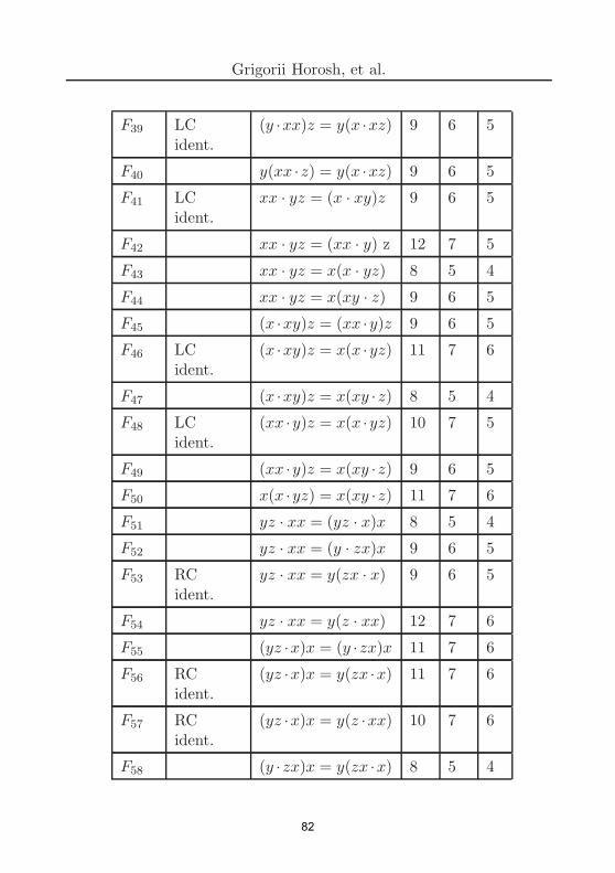
Grigorii Horosh, et al.
F39 LCident.
(y ·xx)z = y(x ·xz) 9 6 5
F40 y(xx ·z) = y(x ·xz) 9 6 5
F41 LCident.
xx · yz = (x · xy)z 9 6 5
F42 xx · yz = (xx · y) z 12 7 5
F43 xx · yz = x(x · yz) 8 5 4
F44 xx · yz = x(xy · z) 9 6 5
F45 (x ·xy)z = (xx ·y)z 9 6 5
F46 LCident.
(x ·xy)z = x(x ·yz) 11 7 6
F47 (x ·xy)z = x(xy ·z) 8 5 4
F48 LCident.
(xx ·y)z = x(x ·yz) 10 7 5
F49 (xx ·y)z = x(xy ·z) 9 6 5
F50 x(x ·yz) = x(xy ·z) 11 7 6
F51 yz · xx = (yz · x)x 8 5 4
F52 yz · xx = (y · zx)x 9 6 5
F53 RCident.
yz · xx = y(zx · x) 9 6 5
F54 yz · xx = y(z · xx) 12 7 6
F55 (yz ·x)x = (y ·zx)x 11 7 6
F56 RCident.
(yz ·x)x = y(zx ·x) 11 7 6
F57 RCident.
(yz ·x)x = y(z ·xx) 10 7 6
F58 (y ·zx)x = y(zx ·x) 8 5 4
82

On groupoids with classical Bol-Moufang type identities
F59 (y ·zx)x = y(z ·xx) 9 6 5
F60 y(zx ·x) = y(z ·xx) 9 6 5
References
[1] Reza Akhtar, Ashley Arp, Michael Kaminski, Jasmine Van Exel, DavianVernon, and CoryWashington. The varieties of Bol-Moufang quasigroupsdefined by a single operation. Quasigroups Related Systems, 20(1), pp.1–10, 2012.
[2] V.D. Belousov. Foundations of the Theory of Quasigroups and Loops.Nauka, Moscow, 1967. (in Russian).
[3] Vladimir Chernov, Alexander Moldovyan, and Victor Shcherbacov. Onsome groupoids of order three with Bol-Moufang type of identities. InProceedings of the Conference on Mathematical Foundations of Informat-
ics MFOI2018, July 2-6, 2018, Chisinau, pp. 17–20, Chisinau, Moldova,2018.
[4] Vladimir Chernov, Alexander Moldovyan, and Victor Shcherbacov. Onsome groupoids of small orders with Bol-Moufang type of identities, 2018.arXiv:1812.02511.
[5] Vladimir Chernov, Nicolai Moldovyan, and Victor Shcherbacov. On somegroupoids of small order. In The Fourth Conference of Mathematical So-
ciety of the Republic of Moldova dedicated to the centenary of Vladimir
Andrunachievici (1917-1997), June 28 - July 2, 2017, Chisinau, Pro-
ceedings CMSM4’, pp. 51–54, Chisinau, Moldova, 2017.
[6] B. Cote, B. Harvill, M. Huhn, and A. Kirchman. Classification of loopsof generalized Bol-Moufang type. Quasigroups Related Systems, 19(2),pp. 193–206, 2011.
[7] Andreas Distler and Tom Kelsey. The semigroups of order 9 and theirautomorphism groups. Semigroup Forum, 88(1), pp. 93–112, 2014.
[8] F. Fenyves. Extra loops. II. On loops with identities of Bol-Moufangtype. Publ. Math. Debrecen, 16, pp. 187–192, 1969.
83

Grigorii Horosh, et al.
[9] Grigorii Horosh, Victor Shcherbacov, Alexandru Tcachenco, and TatianaYatsko. On some groupoids with Bol-Moufang type identities. In Proceed-
ings of the 5-th Conference on Mathematical Foundations of Informatics,
MFOI 2019, July 3-6, pp. 149–158, Iasi, Romania, July 2019.
[10] T.G. Jaıyeola, E. Ilojide, M. O. Olatinwo, and F. Smarandache. On theClassification of Bol-Moufang Type of Some Varieties of Quasi Neutro-sophic Triplet Loop (Fenyves BCI-Algebras). Symmetry, 10, pp. 1–16,2018. doi:10.3390/sym10100427.
[11] K. Kunen. Quasigroups, loops and associative laws. J. Algebra, 185(1),pp. 194–204, 1996.
[12] B. V. Novikov. On decomposition of Moufang groupoids. Quasigroups
and related systems, 16(1), pp. 97–101, 2008.
[13] H.O. Pflugfelder. Quasigroups and Loops: Introduction. HeldermannVerlag, Berlin, 1990.
[14] J. D. Phillips and Petr Vojtechovsky. The varieties of loops of Bol-Moufang type. Algebra Universalis, 54(3), pp. 259–271, 2005.
[15] S. Satoh, K. Yama, and M. Tokizawa. Semigroups of order 8. Semigroup
forum, 49, pp. 7–29, 1994.
[16] Victor Shcherbacov. Elements of Quasigroup Theory and Applications.CRC Press, Boca Raton, 2017.
[17] Wikipedia. Semigroup with two ele-ments, 2015. https://en.wikipedia.org/wiki/Semigroup with two elements.
Grigorii Horosh1, Victor Shcherbacov2, Alexandr Tcachenco3, Tatiana Yatsko4
1Ph.D. Student/Vladimir Andrunakievich Institute of Mathematics and ComputerScience, MoldovaE–mail: [email protected]
2Principal Researcher/Vladimir Andrunakievich Institute of Mathematics and Com-puter Science, MoldovaE–mail: [email protected]
3Master Student /Vladimir Andrunakievich Institute of Mathematics and ComputerScience, MoldovaE–mail: [email protected]
4Master Student/Shevchenko Transnistria State UniversityE–mail: [email protected]
84

Proceedings of the Fifth Conference of Mathematical Society of Moldova
IMCS-55, September 28 - October 1, 2019, Chisinau, Republic of Moldova
On functionally completeness of quasigroups
Izbash Olga, Izbash Vladimir
Abstract
A continuum of nonisomorphic functionally complete quasi-groups is constructed.
Keywords: functionally complete algebra, functionally com-plete quasigroups , monoquasigroups.
By a functionally complete algebra A we mean a finite algebra withunderlying set A and with basic operations f1, f2, ..., fk such that forevery nonnegative integer n and for every function f : An → A thereis a polynomial expression p(x1, x2, ..., xn) over A such that for everyn-tuple (a1, a2, ..., an) we have p(a1, a2, ..., an) = f(a1, a2, ..., an), thatis for each n all functions f : An → A are definable in terms of theoperations f1, f2, ..., fk. Every functionally complete algebra with afinite signature has no more than countable cardinality.
No semigroup (in particular, no group) can be functionally completedue to the fact that in every finite semigroup there is an idempotent. Noloop, no ring can also be functionally complete. Functionally completequasigroups not loops exist. Functionally complete quasigroups are ofgreat importance in the context of cryptographic applications. One ofthe oldest algebraic questions, equally important in computer science,is to decide whether or not an equation or a system of equations has asolution over an algebra. For every finite functionally complete algebrathis problem is in NP. In [1] it is proved that a finite algebra (A,ω)with a single operation is complete if and only if it has no propersubalgebras, automorphisms or congruences.
In [2] the following theorem is proved:
c©2019 by Izbash Olga, Izbash Vladimir
85

Izbash Olga, Izbash Vladimir
Theorem. a) Any quasigroup (Q, ·) for which 2 ≤ |Q| ≤ ℵ0 is isotopic
to some quasigroup without subquasigroups and congruences. b) Any
quasigroup (Q, ·) for which 5 ≤ |Q| ≤ ℵ0 is isotopic to some quasigroup
without subquasigroups, automorphisms and congruences.
It is also shown that there is a continuum of nonisomorphic quasi-groups without subquasigroups, without automorphisms and withoutcongruences. All these quasigroups are functionally complete.
References
[1] G. Rousseau. Completeness in finite algebras with a single opera-
tion. Proceedings of the American Mathematical Society, vol. 18,1967, pp. 1009–1013.
[2] 6. V. Izbash. Monoquasigroups without congruences and automor-
phisms. Izv. Akad. Nauk R. Moldova. Mathematica, 1992, no. 4,pp. 66–76.
Izbash Olga1, Izbash Vladimir2
1 Vladimir Andrunachievici Institute of Mathematics and Computer ScienceE–mail: [email protected]
2Vladimir Andrunachievici Institute of Mathematics and Computer ScienceE–mail: [email protected]
86

Proceedings of the Fifth Conference of Mathematical Society of Moldova
IMCS-55, September 28 - October 1, 2019, Chisinau, Republic of Moldova
Group-theoretic-free proof of Hall’s theorem
about finite sharply 2-transitive permutation
group
Eugene Kuznetsov
Abstract
In this article a scheme of group-theoretic-free proof of well-known Hall’s theorem about description of finite sharply 2-transitive permutation group is given.
Keywords: sharply 2-transitive permutation group, looptransversals, normal subgroup.
1 Introduction
In the theory of finite multiply transitive permutation groups the M.Hall’s theorem is well-known [4]. The proof of this theorem in his bookis group-theoretic. The author of this article will show the anotherproof of this theorem without using the group theory. The scheme ofthe loop-theoretic proof of the Hall’s theorem will be given below.
2 Definitions
Definition 2.1. A set M of permutations on a set X is called sharply
2-transitive, if for any two pairs (a, b) and (c, d) of different elements
from X there exists a unique permutation α ∈ M satisfying the follow-
ing conditions
α(a) = c, α(b) = d.
c©2019 by Eugene Kuznetsov
87

Eugene Kuznetsov
Definition 2.2. [11] Let G be a group and H be its subgroup. Let
Hii∈E be the set of all left cosets in G to H. A set T = tii∈E of
representativities of the left (right) cosets (by one from each coset Hi,
i.e. ti ∈ Hi) is called a left generalized transversal in G to H.
Definition 2.3. [1] A left generalized transversal T = tii∈E in G to
H which satisfies the following conditions: ti0 = e for some i0 ∈ E and
H = H1, is usually called a left transversal in G to H.
Definition 2.4. Let T = tii∈E be a left generalized transversal in G
to H. Define the following operation on the set E:
x(T )
· y = z ⇔ txty = tzh, h ∈ H.
Theorem 1. For an arbitrary left generalized transversal T = tii∈Ein G to H the following statements are true:
1. There exists an element a0 ∈ E such that the system
(
E,(T )
· , a0
)
is a left quasigroup with right unit a0.
2. If T = tii∈E is a left transversal in G to H, then the system(
E,(T )
· , 1
)
is a left loop with unit 1.
3 Transversals with isotopic and isomorphic
transversal operations
Theorem 2. [11] For an arbitrary left generalized transversal T =tii∈E in G to H the following statements are true:
1. If P = pii∈E is a left generalized transversal in G to H such
that for every x ∈ E:
P = Th0, px′ = txh0,
88

Group-theoretic-free proof ...
where h0 ∈ H is an arbitrary fixed element, then the transver-
sal operation
(
E,(P )
·
)
is isotopic to the transversal operation(
E,(T )
·
)
.
2. If S = sii∈E is a left generalized transversal in G to H such
that for every x ∈ E:
S = πT, sx′ = πtx,
where π ∈ G is an arbitrary fixed element, then the transversal op-
eration
(
E,(S)
·
)
is isotopic to the transversal operation
(
E,(T )
·
)
.
Lemma 3.1. [8] Let T = txx∈E be a fixed loop transversal in G to
H and h0 ∈ NSt1(SE)(H). Define the set of permutations:
px′
def
= h−1
0txh0 ∀x ∈ E.
Then
1. P = px′
x′∈E
is a loop transversal in G to H;
2. The transversal operations
(
E,(P )
· , 1
)
and
(
E,(T )
· , 1
)
are iso-
morphic, and the isomorphism is set up by the mapping ϕ(x) =h0(x).
Lemma 3.2. [10] Let T = txx∈E be a fixed loop transversal in G to
H. Let h0 ∈ NSt1(SE)(H) be an element such that:
tx′
def
= h−1
0txh0 ∀x ∈ E.
Then ϕ ≡ h0 ∈ Aut
(
E,(T )
· , 1
)
.
89

Eugene Kuznetsov
4 A finite sharply 2-transitive group of permu-
tations degree n
Theorem 3. Let G be a sharply 2-transitive permutation group on a
finite set of symbols E, i.e.
1. G is a 2-transitive permutation group on E;
2. only identity permutation id fixes two symbols from the set E.
Then
1. the identity permutation id with the set of all fixed-point-free per-
mutations from the group G forms a transitive invariant subgroup
A in the group G;
2. group G is isomorphic to the group of linear transformations
GK = α |α(x) = x · a+ b, a, b ∈ E, a 6= 0
of a some near-field K = 〈E,+, ·, 0, 1〉.
5 A scheme of my proof of Hall’s Theorem
Lemma 5.1. [7] Let G be a sharply 2-transitive permutation group of
degree n on a set E. Then the set T of all fixed-point-free permutations
from G with the identity permutation id form a unique loop transversal
in G to H = St0(G) = α ∈ G|α(0) = 0, 0 ∈ E.
Lemma 5.2. Let T be the loop transversal in G to H from the previous
Lemma. Then the following propositions are true:
1. ∀a ∈ E the set Sa = T · t−1a (where ta ∈ T ) is a loop transversal
in G to H.
2. ∀a ∈ E the set Ra = ta · T (where ta ∈ T ) is a loop transversal
in G to H.
90

Group-theoretic-free proof ...
Lemma 5.3. The transversal T from the previous Lemmas is a group
transversal in G to H.
Lemma 5.4. 1. The group transversal operation (T, ·) has a sharply
transitive automorphism group.
2. The group (T, ·) is a primary cyclic group of order n = pm, p is
a prime number.
References
[1] R. Baer. Nets and groups.1. Trans Amer. Math. Soc., vol. 46, 1939,pp. 110–141.
[2] F. Bonetti, G. Lunardon, K. Strambach. Cappi di permutazionni,
Rend. math., vol. 12, 1979, no. 3–4, pp. 383–395.
[3] I. Burdujan. Some remarks about geometry of quasigroups (Rus-sian), Mat. Issled., Chishinau, ”Shtiintsa”, vol. 39, 1976, pp. 40–53.
[4] M. Hall. Group theory,(Russian) IL, Moscow, 1962.
[5] E.A. Kuznetsov. Sharply 2-transitive permutation groups.1, Quasi-groups and related systems, vol. 2, 1995, pp. 83–100.
[6] E.A. Kuznetsov. Transversals in groups.2.Loop transversals in a
group by the same subgroup, Quasigroups and related systems, vol.6, 1999, pp. 1–12.
[7] Kuznetsov E. A loop transversal in a sharply 2-transitive permuta-
tion loop. Bulletin of the Academy of Sciences of Moldova, Math-ematics, no. 3(49), 2005, pp. 101–114.
[8] E.A. Kuznetsov, S.V. Botnari. Invariant transformations of loop
transversals. 1. The case of isomorphism. Bulletin of the Academyof Sciences of Moldova, Mathematics, no. 1(62), 2010, pp. 65–76.
91

Eugene Kuznetsov
[9] E.A. Kuznetsov, S.V. Botnari. Invariant transformations of loop
transversals.2. The case of isotopy, Bulletin of the Academy ofSciences of Moldova, Matematica, no. 3(70), 2012, pp. 72–80.
[10] E.A. Kuznetsov, S.V. Botnari. Invariant transformations of
loop transversals.1a. The case of automorphism, Bulletin of theAcademy of Sciences of Moldova, Matematica, no. 1(74), 2014,pp. 113–116.
[11] E.A. Kuznetsov. General form transversals in groups, Bulletin ofthe Academy of Sciences of Moldova, Matematica, no. 2(81), 2016,pp. 93–106.
Eugene Kuznetsov
Vladimir Andrunachievici Institute of Mathematics and Computer Science,Chisinau, MoldovaE–mail: [email protected]
92

Proceedings of the Fifth Conference of Mathematical Society of Moldova
IMCS-55, September 28 - October 1, 2019, Chisinau, Republic of Moldova
On the theory of finite crystallographic groups
of cyclical Wp-symmetry
Alexandru Lungu
Abstract
In this paper there are studied the groups of Wp-symmetrytransformations of the geometrical finite figures regularly weightedby ”physical” scalar tasks. Some finite crystallographic groupsof cyclical Wp-symmetry are analysed.
Keywords: groups, symmetry, quasi-homeomorphisms, wreathproducts.
1 Introduction
Wp-symmetry [1-5] is one of the main generalizations of classical sym-metry. In this case the transformations of the qualities, attributed tothe points, essentially depend on the choice of points. The set of trans-formations of Wp-symmetry of the given “indexed” geometrical figure
F(N) forms a group G
(Wp) with the operation g
(wi)
ig
(wj)
j= g
(wk)
k, where
gk = gigj , wk = wgj
iwj and w
gj
i(gs) = wi(gjgs). The group G
(Wp) is
called major, minor or V-middle if w0 < V = W′ = W,w0 = V < W
′ =W or w0 < V < W
′ = W , respectively, where w0 is the unit of groupW , W ′ = w|g(w) ∈ G
(Wp) ⊆ W and V = G
(Wp) ∩W = G
(Wp) ∩W
′ isthe subgoup of W -identical transformations of the group G
(Wp). If W ′
is a non-trivial subgroup of W , then the group G(W
p) is called W
′-semi-major, W ′-semi-minor or (W ′
, V )-semi-middle according to the caseswhen w0 < V = W
′, w0 = V < W
′ or w0 < V < W′. If W ′ ⊂ W ,
but W ′ is not a group, the group G(W
p) is called W
′-pseudo-minor or(W ′
, V )-pseudo-middle when w0 = V ⊂ W′ or w0 < V ⊂ W
′.
c©2019 by Alexandru Lungu
93

Alexandru Lungu
2 About general properties of the groups of
Wp-symmetry
The cristallographic punctual groups G(W
p) of Wp-symmetry are sub-
groups of left direct wreath product of initial group P with the gener-ating group G, accompanied with a fixed isomorphism ϕ : G → AutW
(where W is the direct product of isomorphic copies of group P whichare indexed by elements of group G). We will mention that the majorWp- symmetry group is constructed in the form of the left-direct wreathproduct of the initial definition group P with the generator group G,accompanied with a fixed isomorphism ϕ : G → AutW .
Of all the specific properties of crystallographic punctual groups ofWp-symmetry, that relate to their overall structure, we shall mentiononly main ones.
1) The application µ of the group G(Wp) onto the set W
′ =w|g(w) ∈ G
(Wp) ⊆ W with the unit w0 of the group W by the rule
µ[g(w)] = w is a left quasi-homomorphism with the kernel H, where His the symmetry subgroup in G
(Wp).
2) The application ϕ of the group G(W
p) onto the group G by the
rule ϕ[g(w)] = g is homomorphic with the kernel V .
3) Vg = wV w
−1 for all components g and w of transformationsg(w) of group G
(Wp).
4) Any element of the class of residues Hg is combined in pairs witheach element of residues class wV , but the elements of different classesHgi and Hgj are combined with the elements of different classes wiV
and wjV , respectively.
5) The group G(W
p) contains as its subgroup a group G
(W1)
1of P -
symmetry (which is determined by initial group P of permutations,where W1 ≤ DiagW ∼= P and W1 ⊂ W
′) from the family with the gen-erating group G1 (G1 ≤ G), with the symmetry subgroup H (whereH E G1 but H 6= G) and with the subgroup V1 of W -identical trans-formations (where V1 = V ∩DiagW ).
94

Finite crystallographic groups of cyclical Wp-symmetry
3 On methods of deriving groups of Wp-symmetry
of different types
Any W′-semi-major finite group of Wp-symmetry with initial group P
and generating group G can be derived from G and P by the followingsteps: 1) we construct the direct product W of isomorphic copies ofthe group P which are indexed by elements of G; 2) we construct for
each g of G the automorphism
g of the group W , which acts on theelements w in W as g-moving to the left of the components; 3) wefind in W such non trivial subgroups W
′ which verify the conditions
g (W ′)W ′ = W′; 4) we combine pairwise each g of group G with
each w of subgroup W′; 5) we introduce into the set of all these pairs
the operation giwi gjwj = gkwk, where gk = gigj , wk = wgj
iwj and
wgj
i(gs) = wi(gjgs).
Any W′-semi-minor finite group of Wp-symmetry with initial group
P , generating group G and symmetry subgroup H can be derived fromG and P by the following steps: 1) we construct the left direct productW of isomorphic copies of the group P , indexed by elements of G;
2) we construct for each g of G the automorphism
g of the groupW , which acts on the elements w in W as g-moving to the left ofthe components; 3) we find in W such non trivial subgroups W ′ which
verify the conditions
g (W ′)W ′ = W′; 4) we construct an exact natural
left quasi-homomorphism µ with the kernel H of the group G onto thesubgroup W
′ by the rule µ(Hg) = w ; 5) we combine pairwise each g
of class Hg with w= µ(Hg); 6) we introduce into the set of all thesepairs the operation giwi gjwj = gkwk, where gk = gigj , wk = w
gj
iwj
and wgj
i(gs) = wi(gjgs).
In the case of the pseudo-minor groups the method of deducingthem from the given groups G and P is completely analogous to thatfor the semi-minor groups with the only difference: in this case W
′ isnot a non-trivial subgroup but is a subset that contains the unit of thegroup W as an element.
95

Alexandru Lungu
4 Conclusion
From the non trivial crystallographic punctual groups G (cyclic andnon cyclicals) with the order 2,3,4, 6 and the group P (P ∼= C2), weobtained: 1) 14 major groups, 2) 39 W
′-semi-major groups; 3) 15 semi-minor groups, 4) 41 pseudo-minor groups of Wp-symmetry.
Acknowledgments. The project 15.817.02.26F has supportedpart of the research for this paper.
References
[1] V.A. Koptsik and I.N. Kotsev. To the theory and classification
of color symmetry Groups. II. W -symmetry. (Russian). OIYI Re-ports, R4-8068, Dubna, 1974.
[2] A.P. Lungu. Classification of groups of W -symmetry. Studies inmodern algebra and geometry, pp. 79–84, Chisinau: Shtiintsa,1983. (in Russian).
[3] A. Lungu. The general theory of Wp-symmetry groups. (Roma-nian). Symposium septimum Tiraspolense ”Generalis topologiaeet suae applicationum”. 1996. Chisinau: Tehnica UTM, pp. 140–143.
[4] A. Lungu. On some properties of Wp-symmetry groups. First Con-ference of the Mathematical Society of the Republic of Moldova,Chisinau, august 16-18, 2001. Abstracts. pp. 90–91.
[5] A. Lungu. Grupuri punctuale cristalografice de Wp-simetrii ciclice.Studia Universitatis Moldaviae. Revista stiintifica. Seria “Stiinteexacte si economice”, Chisinau, CEP USM. no. 2 (102), 2017, pp.3–12. (in Romanian).
Alexandru Lungu
Chisinau/State University of MoldovaE–mail: [email protected]
96

Proceedings of the Fifth Conference of Mathematical Society of Moldova
IMCS-55, September 28 - October 1, 2019, Chisinau, Republic of Moldova
Construction of linear binary codes using
orthogonal systems of Latin squares
Nadezhda Malyutina, Alexei Shcherbacov,
Victor Shcherbacov
Abstract
Using orthogonal systems of Latin squares we construct linearbinary codes with the length of code words (n2+(r+2)n) whichcan correct up to r+2
2errors, where r ∈ N.
Keywords: quasigroup, Latin square, binary code, vectorspace, error, orthogonal binary groupoids.
2000 Mathematics Subject Classification: 20N05 05B1594B05 94B65
1 Introduction
Necessary information about linear codes, quasigroups and their or-thogonality can be found in [2, 4, 5, 1, 6].
Let the incoming binary information be divided into blocks of con-stant length n
2 (binary vectors). In total there are 2n2
possible differentblocks. We can define on this set of blocks the operations + (additionof vectors) and · (multiplication of vectors by a number from the fieldGF (2)). This set with these operations is transformed into linear vectorspace E
n2
of dimension n2 over the field GF (2).
We can associate with this vector space a linear binary code C withcode words of length n
2+(2+r)n, i.e., we can define linear vector spaceE
n2+(2+r)n which contains 2n
2
code words.
c©2019 by Nadezhda Malyutina, Alexei Shcherbacov, Victor Shcherbacov
97

Nadezhda Malyutina, et al.
2 Construction
The check matrix H of this code C [6, 1] we construct as follows.
Suppose that we have r mutually (in pairs) orthogonal Latinsquares L1, L2, . . . , Lr and two selectors F and E defined on the set1, 2, . . . , n.
F =
1 1 . . . 12 2 . . . 2...
.... . .
...n n . . . n
, E =
1 2 . . . n
1 2 . . . n
......
. . ....
1 2 . . . n
Notice, that evaluations of the number of mutually (in pairs) or-thogonal Latin squares is given in [3, 5]. For example, if q is prime,then this number is equal to (q − 1).
We put in correspondence to every table from the setK = F,E,L1,
L2, . . . , Lr a rectangular matrix D of size n×n2 as follows. Using table
of size n × n we build n matrices C1, C2, . . . , Cn of size n × n: matrixCi consists of units at the locations of the element i in the matrix fromthe set K and zeros in other places, i = 1, 2, . . . , n.
With each of the matrices D we associate row vectors vi, i =1, 2, . . . , n which consist of the rows of the matrix D, written one afteranother in order, starting from the first. The length of the vector vi isn2.
We associate each of the matrices F,E,L1, . . . , Lr with matricesF
′, E
′, L
′
1, . . . , L
′
rin the way described above.
We form the check matrixH, writing the matrices F ′, E
′, L
′
1, . . . , L
′
r
one under the other, and add the identity matrix to the resulting ma-trix on the right, i.e., we add a square matrix Em ( m = (r + 2)n))whose order is equal to the total number of rows in all matricesF
′, E
′, L
′
1, . . . , L
′
r.
98

Linear binary codes
H =
E′
F′
L′
1
L′
2
...L′
r
Em
.
The matrix H has dimension ((r + 2)n)× (n2 + (r + 2)n).
The coding is carried out according to the rule: each vector a ofzeros and units of length n
2 is associated with a vector b = aG, whereGH
T = 0, i.e., G is the generating code matrix.
Hamming distance of this code is d = r+3. Hence the code is ableto correct up to r+2
2errors.
Due to the pairwise orthogonality of the squares F,E,L1, . . . , Lr
for each of the information symbols αi, (i = 1, 2, . . . , n2) we obtain inaccordance with the matrix H r+2 orthogonal checks, which makes itpossible to fix r+2
2errors.
Example 1. We take matrices over the set 0, 2. It is easy to check
that the cyclic group of order 3 (Z3,+), quasigroup (Z3, ) of the form
x y = x + 2 · y, where x, y ∈ R3, (here (R3,+, ·) means the ring
residues modulo 3), selectors F and E are orthogonal in pairs. The
matrix D(Z3,+) has the following form:
D(Z3,+) =
1 0 0 0 1 0 0 0 10 0 1 1 0 0 0 1 00 1 0 0 0 1 1 0 0
.
In this case r = 2, m = (2+2)3 = 12. The matrix H has dimension
12 × 21. The constructed code can correct two errors. The length of
code words is equal to 21. The generating matrix G of this code has
dimension 9× 21. This code contains 2 9 = 512 code words.
99

Nadezhda Malyutina, et al.
3 Concluson
Taking into consideration that concept of orthogonality admits differ-ent generalization in various directions we can say that the describedconstruction can be generalised and improved.
References
[1] M. N. Arshinov and L. E. Sadovskii. Codes and Mathematics.Nauka, Moscow, 1983. (in Russian).
[2] V.D. Belousov. Foundations of the Theory of Quasigroups and
Loops. Nauka, Moscow, 1967. (in Russian).
[3] J. Denes and A. D. Keedwell. Latin Squares and their Applications.Academiai Kiado, Budapest, 1974.
[4] H.O. Pflugfelder. Quasigroups and Loops: Introduction. Helder-mann Verlag, Berlin, 1990.
[5] Victor Shcherbacov. Elements of Quasigroup Theory and Applica-
tions. CRC Press, Boca Raton, 2017.
[6] F. I. Solov’eva. Introduction to the Code Theory. Novosibirsk StateUniversity, 2006. (in Russian).
Nadezhda Malyutina1, Alexei Shcherbacov2, Victor Shcherbacov3
1Ph.D. Student/Dimitrie Cantemir State University, MoldovaE–mail: [email protected]
2M.Sc., Theoretical Lyceum C. Sibirschi, MoldovaE–mail: [email protected]
3Principal Researcher/Vladimir Andrunakievich Institute of Mathematics and Com-puter Science of MoldovaE–mail: [email protected]
100

Proceedings of the Fifth Conference of Mathematical Society of Moldova
IMCS-55, September 28 - October 1, 2019, Chisinau, Republic of Moldova
On Defining 4-Dimensional Finite
Non-Commutative Associative Algebras Over
GF (2s)
Dmitrii Moldovyan, Alexander Moldovyan,
Victor Shcherbacov
Abstract
Finite non-commutative associative algebras are attractive ascarriers of the post-quantum public-key cryptoschemes. The 4-dimensional algebras defined over the fields GF (2s) representpractical interest to provide higher performance. Properties ofseveral different algebras of such type are considered.
Keywords: non-commutative algebra, 4-dimensional asso-ciative algebra, post-quantum cryptoscheme.
1 Introduction
The m-dimensional finite non-commutative associative algebras(FNAAs; m ≥ 4) represent practical interest as carriers of the hiddendiscrete logarithm problem (HDLP) that was proposed as the basicprimitive of the public-key post-quantum cryptoschemes [1, 2]. The useof the 4-dimensional FNAA allows one to get higher performance of thecryptographic algorithms and protocols. To provide cheaper hardwareimplementation it is attractive to use the 4-dimensional FNAA set overthe fields GF (2s). The finite algebra of quaternions represents the wellknown case of the 4-dimensional FNAA set over the fieldsGF (p), wherep ≥ 3 is a prime, however there exists no quaternion algebra set overGF (2s). This is due to the fact that there exists only one square root
c©2019 by Dmitrii Moldovyan, Alexander Moldovyan, Victor Shcherbacov
101

Dmitrii Moldovyan, et al.
from an arbitrary fixed element of the field GF (2s) for arbitrary fixednon-negative integer s.
In this paper we consider several different types of the 4-dimensionalFNAA and some of their properties.
2 Preliminaries
The finite m-dimensional vector space with the additionally definedoperation of multiplying arbitrary two vectors, which is distributiverelatively the addition operation, represents the algebraic structurecalled the m-dimensional finite algebra. Suppose e0, e1, ... em−1
are the basis vectors. The vector A of a vector space defined overthe finite field GF (2s) can be denoted in the following two forms:A = (a0, a1, . . . , am−1) and A = a0e0 + a1e1 + · · · + am−1em−1, wherea0, a1, . . . , am−1 ∈ GF (2s) are called coordinates. The multiplicationoperation (denoted as ) of two vectors A and B =
∑
m−1
j=0bjej is usu-
ally defined as follows
A B =
m−1∑
i=0
m−1∑
j=0
aibj(ei ej),
where each of the products ei ej is to be substituted by a single-component vector λek, where λ ∈ GF (2s) is called structural constant,indicated in the respective cell of so called basis vector multiplicationtable (BVMT). It is usually assumed that the intersection of the ithrow and jth column defines the cell indicating the value of the producteiej . If the defined vector multiplication is non-commutative and asso-ciative, then we have FNAA. To define associative vector multiplicationone should compose the BVMT that defines associative multiplicationof all possible triples of the basis vectors (ei, ej , ek):
(ei ej) ek = ei (ej ek) .
For arbitrary fixed natural number s ≥ 2 a set of all binary polynomialsof the degree d < s, in which the multiplication of two polynomials is
102

On Defining 4-dimensional associative algebras
defined modulo an irreducible binary polynomial ρ of the degree s,
represents a field GF (2s). One can set different fields GF (2s) selectingdifferent values ρ, all of such fields being isomorphic.
3 The FNAAs with global two-sided unit
The BVMT shown as Table 1 sets the non-commutative multiplica-tion operation of the 4-dimensional vectors that are defined over anarbitrary fixed finite field, including the fields GF (2s). The respec-tive 4-dimensional FNAA contains the global two-sided unit E =(e0, e1, e2, e3) that is described as follows:
E =
(
σ
λσ − 1,
1
1− λσ,
1
1− λσ,
λ
λσ − 1
)
. (1)
For some invertible vector A = (a0, a1, a2, a3) the equation X
A = E, where X = (x0, x1, x2, x3) is the unknown value, has solutionX = A
−1 that can be obtained solving the following two independentsystems of two linear equations with the unknowns (x0, x1) and (x2, x3)correspondingly:
(λa0 + a2) x0 + (a0 + σa2)x1 = e0;
(λa1 + a3) x0 + (a1 + σa3)x1 = e1;(2)
(λa0 + a2) x2 + (a0 + σa2)x3 = e2;
(λa1 + a3) x2 + (a1 + σa3)x3 = e3.(3)
Each of the systems (2) and (3) has the same main determinant ∆A :
∆A = (λa0 + a2) (a1 + σa3)− (λa1 + a3) (a0 + σa2) =
= (1− λσ) (a1a2 − a0a3) .(4)
From the condition ∆A 6= 0 we have the following invertibility conditionof the elements of the considered 4-dimensional FNAA:
a1a2 6= a0a3. (5)
103

Dmitrii Moldovyan, et al.
Table 1. The BVMT setting the 4-dimensional FNAA over GF (2s)(λσ 6= 1).
e0 e1 e2 e3
e0 λe0 λe1 e0 e1
e1 e0 e1 σe0 σe1
e2 λe2 λe3 e2 e3
e3 e2 e3 σe2 σe3
Another 4-dimensional FNAA can be set over the fields GF (2s)with the BVMT shown in Table 2 that is constructed using the unifiedmethod for defining the FNAAs of arbitrary even dimensions [3]. TheFNAA defined by Table 2, where τ 6= 1, contains the global bi-sidedunit
E =
(
1
1− τ,
1
1− τ,
τ
τ − 1,
1
τ − 1
)
.
Vectors A = (a0, a1, a2, a3), coordinates of which satisfy the condition
a0a1 6= a2a3, (6)
are invertible.From the invertibility conditions (5) and (6) one can derive the
following formula for number Ω of the invertible elements in each ofthe described 4-dimensional FNAAs:
Ω = 2s (2s − 1)2 (2s + 1) . (7)
4 The FNAAs containing the set of 22s global
right-sided units
Table 3 sets the 4-dimensional FNAA containing no global two-sidedunit. This algebra is characterized in that it contains a large set of
104
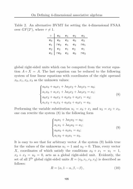
On Defining 4-dimensional associative algebras
Table 2. An alternative BVMT for setting the 4-dimensional FNAAover GF (2s), where τ 6= 1.
e0 e1 e2 e3
e0 e0 e3 e0 e3
e1 τe2 e1 e2 τe1
e2 e2 e1 e2 e1
e3 τe0 e3 e0 τe3
global right-sided units which can be computed from the vector equa-tion A X = A. The last equation can be reduced to the followingsystem of four linear equations with coordinates of the right operandx0, x1, x2, x3 as the unknown values:
a0x0 + a0x1 + λa2x2 + λa2x3 = a0;
a1x0 + a1x1 + λa3x2 + λa3x3 = a1;
a0x2 + a0x3 + a2x0 + a2x1 = a2;
a1x2 + a1x3 + a3x0 + a3x1 = a3.
(8)
Performing the variable substitution u1 = x0 + x1 and u2 = x2 + x3,
one can rewrite the system (8) in the following form
a0u1 + λa2u2 = a0;
a1u1 + λa3u2 = a1;
a0u2 + a2u1 = a2;
a1u2 + a3u1 = a3.
(9)
It is easy to see that for arbitrary vector A the system (9) holds truefor the values of the unknowns u1 = 1 and u2 = 0. Thus, every vectorX, coordinates of which satisfy the conditions x0 + x1 = u1 = 1,x2 + x3 = u2 = 0, acts as a global right-sided unit. Evidently, theset of all 22s global right-sided units R = (r0, r1, r2, r3) is described asfollows:
R = (α, 1 − α, β,−β) , (10)
105

Dmitrii Moldovyan, et al.
Table 3. The BVMT setting the 4-dimensional FNAA with 22s globalright-sided units (λ ∈ GF (2s); λ 6= 0).
e0 e1 e2 e3
e0 e0 e0 e2 e2
e1 e1 e1 e3 e3
e2 e2 e2 λe0 λe0
e3 e3 e3 λe1 λe1
where α, β ∈ GF (2s).
One can show that every vector A = (a0, a1, a2, a3), coordinates ofwhich satisfy the condition
(a0 + a1)2 = λ (a2 + a3)
2, (11)
is a locally invertible element of the considered FNAA, i. e., a localtwo-sided unit EA relates to such vector A. Besides, the vector A is agenerator of finite cyclic group contained in the algebra. Evidently, thelocal unit EA is the group unit of the mentioned cyclic group.
Local two-sided units are contained in the set (10) and every globalright-sided unit is simultaneously a local two-sided unit relating to someinvertible vector. All invertible vectors relating to some fixed localtwo-sided unit compose a finite multiplicative group. The consideredFNAA is divided into 22s groups, since every global right-sided unitsets a group.
From the condition (11) one can find the number of invertible vec-tors Ω:
Ω = 23s (2s − 1) .
One can show every of the mentioned finite groups has the same orderΩ′. Since every invertible vector is contained only in one of the groups,
we have the following formula for the value Ω′:
Ω′ = 2s (2s − 1) .
106

On Defining 4-dimensional associative algebras
5 On some applications
The FNAAs described in Sections 2 can be used to implement post-quantum digital signature schemes proposed in [4] on the basis of thefinite algebra of quaternions. The FNAAs described in Section 3 can beused as algebraic carrier of post-quantum public key-agreement schemeproposed in [5]. In both cases we will get higher performance of thecryptoschemes.
6 Conclusion
One can propose different types of the BVMT for setting 4-dimensionalFNAAs over the finite fields GF (2s). Using such FNAAs as carries ofthe public-key post-quantum schemes one can get higher perfomanceof the cryptoschemes.
Acknowledgments. The authors thank Referee for valuable re-marks.
References
[1] D.N. Moldovyan. Non-Commutative Finite Groups as Primitive
of Public-Key Cryptoschemes, Quasigroups and Related Systems,2010, vol. 18. no. 2, pp. 165–176.
[2] A.S. Kuzmin, V.T. Markov, A.A. Mikhalev, A.V. Mikhalev, andA.A. Nechaev. Cryptographic Algorithms on Groups and Algebras,Journal of Mathematical Sciences, 2017, vol. 223. vo. 5, pp. 629–641.
[3] N.A. Moldovyan and A.A. Moldovyan. Finite Non-commutative
Associative Algebras as carriers of Hidden Discrete Logarithm
Problem, Bulletin of the South Ural State University. Ser. Mathe-matical Modelling, Programming & Computer Software (BulletinSUSU MMCS), 2019, vol. 12. no. 1, pp. 66–81.
107

Dmitrii Moldovyan, et al.
[4] N. A. Moldovyan and I. K. Abrosimov. Post-quantum elec-
tronic digital signature scheme based on the enhanced form
of the hidden discrete logarithm problem, Vestnik of SaintPetersburg University. Applied Mathematics. Computer Sci-ence. Control Processes, 2019, vol. 15, iss. 2, pp. 212–220.https://doi.org/10.21638/11702/spbu10.2019.205. (In Russian).
[5] D.N. Moldovyan. Post-quantum public key-agreement scheme
based on a new form of the hidden logarithm problem, ComputerScience Journal of Moldova, 2019, vol. 27, no. 1(79), pp. 56–72.
Dmitrii Moldovyan1, Alexander Moldovyan2, Victor Shcherbacov3
1 St. Petersburg Institute for Informaticsand Automation of Russian Academy of SciencesSt. Petersburg, Russian FederationE–mail: [email protected]
2 St. Petersburg Institute for Informaticsand Automation of Russian Academy of SciencesSt. Petersburg, Russian FederationE–mail: [email protected]
3 Institute of Mathematics and Computer ScienceChisinau, MoldovaE–mail: [email protected]
108

Proceedings of the Fifth Conference of Mathematical Society of Moldova
IMCS-55, September 28 - October 1, 2019, Chisinau, Republic of Moldova
Finite Non-commutative Algebras as Carriers of
Post-quantum Public-key Cryptoschemes
Alexandr Moldovyan and Nicolai Moldovyan
Abstract
Hidden logarithm problem defined in finite non-commutativeassociative algebras had been proposed as the base primitiveof the post-quantum public-key cryptoschemes. Different typesof the algebras are considered as the carriers of different post-quantum public-key cryptoschemes. Related research tasks areconsidered.
Keywords: finite non-commutative algebra, associative al-gebra, public-key cryptography, post-quantum cryptoscheme.
1 Introduction
Development of the post-quantum public-key cryptoschemes representsthe modern challenge in the area of applied and theoretic cryptogra-phy [1, 2, 3]. Different forms of the hidden discrete logarithm problem(HDLP) defined over the finite non-commutative associative algebras(FNAAs) were proposed as the base primitive of the post-quantumpublic key-agreement [4, 5, 6] and digital signature schemes [7, 8, 9].
In this report we summarize the current results on application ofthe FNAAs as algebraic carrier of the post-quantum cryptoschemesand some research items connected with the development of the post-quantum cryptographic algorithm and protocols.
2 Preliminaries
For using as cryptographic primitive, the DLP is set in a finite cyclicgroup Γ of the order Ω containing a large prime divisor q as follows:
Y′ = G
x,
c©2019 by Alexandr Moldovyan and Nicolai Moldovyan
109

Alexandr Moldovyan and Nicolai Moldovyan
where Y′ is the public key; G is a generator of the group; and the
non-negative integer x < Ω is the unknown (private key). Findingthe value x, when the values G and Y
′ are known, is called DLP. TheHDLP represents a universal cryptographic primitive on the basis ofwhich different types of the public-key algorithms and protocols weredeveloped, including various cryptographic standards. Unfortunatelythe DLP can be solved in polynomial time on the hypothetic quantumcomputer [10]. The last means the DLP-based cryptoschemes will benot secure in the comming age of quantum computations [11].
To provide security to quantum attacks the HDLP was proposed.The HDLP is defined so that one of the values G and Y
′ or both ofthem are masked (hidden). Thus, it is supposed the HDLP is set insome finite algebraic structure containing a large variety of finite cyclicgroups. The FNAAs suite well as algebraic carriers of the HDLP. Themain contribution to the security is introduced by the exponentiationoperation G
x that is called the base operation. The operation usedto hide the values G and Y
′ are called the masking operations. Toprovide possibility to design the HDLP-based public-key cryptoschemesone should use the masking operations that are mutually commutativewith the base operation. Therefore, the automorphism-map operationsand the homomorphism-map operations are attractive to be applied asmasking operations. Using different types of the masking operationsone can set different versions of the HDLP.
For the first time the HDLP was defined in the finite algebra ofquaternions [4, 12] as follows:
Y = Qw Gx Q−w = α (Gx) , (1)
where Q G 6= G Q; the variable V takes on all values in the quater-nion algebra; α (V ) is the automorphism-map operation. The formof HDLP descibed by the formula (1) was applied to design a publickey-agreement scheme and commutative encryption algorithm [4, 12].However, reducibility of the first form of the HDLP to the DLP in thefinite field GF (p2) was shown in the paper [5].
Recently [7, 13] several new FNAAs and new versions of the HDLP
110

Finite algebras as carriers of post-quantum cryptoschemes
were introduced and used to develop the post-quantum digital signatureprotocols. For example, in the digital signature scheme defined in theFNAA containing global two-sided unit the public key represents thetriple of vectors (Y,Z, T ) defined as follows [13]:
Y = Q Gx Q−1, Z = H G H−1; T = Q E H−1
, (2)
where Q G 6= G Q; H G 6= H Q; E is a randomly selected vectorfrom the set of local units related to the non-invertible vector G. TheHDLP consists in finding the value x in the case, when only the publickey is known.
In the signature scheme defined in the FNAA containing a large setof global left-sided units the public key represents the pair of vectors(Y,Z) defined as follows [7]:
Y = H Gx D, Z = J G T, (3)
where D G 6= GD; D H = L1; D J = L2; T J = L3; L1, L2, andL3 are global left-sided units. The HDLP consists in finding the valuex in the case, when only the values Y and Z are known.
3 Types of the FNAAs suitable for setting the
HDLP
The FNAAs suitable for application as algebraic carriers of the cryp-toschemes based on the HDLP can be classified by type of the maskingoperations that can be potentially used. The masking operations rep-resent some homomorphism-map and automorphism-map operationsand setting the operations of the last two kinds is connected with thetypes of the unit elements contained in a fixed FNAA, therefore them-dimensional FNAAs (m ≥ 4) can be classified by types of the unitsavailable in the frame of the fixed FNAA.
The FNAAs containing the global two-sided unit are attractive forusing them as algebraic carriers of the digital signature and blind digitalsignature schemes. Setting of different types of HDLP is connected withusing the automorphism-map operations.
111

Alexandr Moldovyan and Nicolai Moldovyan
The FNAAs containing the large set of the global single-sided(left-sided or right-sided) units can be applied as algebraic carriers ofthe digital signature and blind digital signature schemes, public key-agreement protocols, public-encryption and commutative-encryptionalgorithms. Setting different types of HDLP is connected with usingthe homomorphism-map operations of two different kinds.
4 Defining the FNAAs of different dimensions
One can define the m-dimensional FNAA for an arbitrary fixed valuem ≥ 2, however, the cases of even dimensions m ≥ 4 represent themain interest for their application as algebraic carriers of the post-quantum cryptoschemes. The non-commutative multiplication opera-tion in the FNAAs is defined with so called basis vector multiplicationtables (BVMTs). For the case m = 4 different BVMTs can be selectedusing the exhaustive-search method that is not efficient for the casesm ≥ 6.
In the last case it is interesting to use some unified methods fordescribing the BVMTs for different values m. The paper [14] considersa method for defining the FNAAs of arbitrary fixed dimension m > 1and general description of the properties of the defined class of algebras.
The paper [7] had introduced a method for defining the FNAAs ofarbitrary even dimension m > 2. Using that method one can define4-dimensional FNAAs with global two-sided unit and 6-dimensionalFNAAs containing sets of the global single-sided units.
The paper [15] had introduced a method for defining the FNAAsof arbitrary even dimension m > 2. Using that method one can define4-dimensional FNAAs with global two-sided unit and 6-dimensionalFNAAs containing sets of the global single-sided units.
Each of the unified methods is introduced as respective mathe-matical formula describing the class of the BVMTs defining the non-commutative associative multiplication operation. One of the meritsof the unified methods for defining the FNAAs is the general proof ofthe associativity property for all given values m.
112

Finite algebras as carriers of post-quantum cryptoschemes
5 Conclusion
Currently the HDLP can be considered as universal post-quantumcryptographic primitive. Different FNAAs are proposed as algebraiccarriers of different forms of the HDLP used to propose candidatesfor post-quantum signature schemes, public key-agreement proptocols,public-encryption and commutative encryption algorithms. The mainresearch task connected with the post-quantum security estimation ofthe proposed candidates consists in the investigation of the reducibilityof different forms of the HDLP to the DLP in a finite field.
Study of the structure of FNAAs and designing new forms of theHDLP are also important research tasks in the area of development ofthe post-quantum cryptoschemes based on computations in FNAAs.
Development of the HDLP-based cryptoschemes using the FNAAsdefined over the finite field GF (2s) represents significant practical in-terest.
References
[1] First NIST standardization conference - April 11–13, 2018.http://prometheuscrypt.gforge.inria.fr/2018-04-18.pqc2018.html
[2] Proceedings of the 7th International Workshop on Post-Quantum Cryp-tography, PQCrypto 2016. Fukuoka, Japan, February 24-26, 2016. Lec-ture Notes in Computer Science series. Springer, 2016, vol. 9606.
[3] Post-Quantum Cryptography. Proceedings of the 7th 9th InternationalConference, PQCrypto 2018, Fort Lauderdale, FL, USA, April 9-11,2018. Lecture Notes in Computer Science series. Springer, 2018, vol.10786.
[4] D.N. Moldovyan. Non-Commutative Finite Groups as Primitive of
Public-Key Cryptoschemes, Quasigroups and Related Systems, vol. 18,no. 2, 2010, pp. 165–176.
[5] A.S. Kuzmin, V.T. Markov, A.A. Mikhalev, A.V. Mikhalev, A.A.Nechaev. Cryptographic Algorithms on Groups and Algebras, Journal ofMathematical Sciences, vol. 223, no. 5, 2017, pp. 629–641.
[6] Moldovyan D.N. Post-quantum public key-agreement scheme based on anew form of the hidden logarithm problem // Computer Science Journal
of Moldova. 2019. Vol. 27. No. 1(79), pp. 56–72.
113

Alexandr Moldovyan and Nicolai Moldovyan
[7] N.A. Moldovyan, A.A. Moldovyan. Finite Non-commutative Associative
Algebras as carriers of Hidden Discrete Logarithm Problem, Bulletin ofthe South Ural State University. Ser. Mathematical Modelling, Program-ming & Computer Software (Bulletin SUSU MMCS), vol. 12. no. 1, 2019,pp. 66–81.
[8] N.A. Moldovyan, I.K. Abrosimov. Post-quantum electronic digital signa-
ture scheme based on the enhanced form of the hidden discrete logarithm
problem, Vestnik of Saint Petersburg University. Applied Mathematics.Computer Science. Control Processes, vol. 15, iss. 2, 2019, p. 212–220.https://doi.org/10.21638/11702/spbu10.2019.205 (In Russian).
[9] N.A. Moldovyan. Finite Non-commutative Associative Algebras for Set-
ting the Hidden Discrete Logarithm Problem and Post-quantum Cryp-
toschemes on its Base, Buletinul Academiei de Stiinte a RepubliciiMoldova. Matematica, no. 1(89), 2019, pp. 71–78.
[10] P.W. Shor. Polynomial-time algorithms for prime factorization and dis-
crete logarithms on quantum computer, SIAM Journal of Computing,vol. 26, 1997, pp. 1484–1509.
[11] S.Y. Yan. Quantum Attacks on Public-Key Cryptosystems, Springer,2014, 207 p.
[12] D.N. Moldovyan, N.A. Moldovyan.Cryptoschemes over hidden conjugacy
search problem and attacks using homomorphisms, Quasigroups RelatedSystems, vol. 18, no. 2, 2010, pp. 177–186.
[13] A.A. Moldovyan, N.A. Moldovyan. Post-quantum signature algorithms
based on the hidden discrete logarithm problem, Computer Science Jour-nal of Moldova, vol. 26, no. 3(78), 2018, pp. 301–313.
[14] A.A. Moldovyan. General Method for Defining Finite Non-commutative
Associative Algebras of Dimension m > 1, Buletinul Academiei de Stiintea Republicii Moldova. Matematica, no. 2(87), 2018, pp. 95–100.
[15] N.A. Moldovyan.Unified Method for Defining Finite Associative Algebras
of Arbitrary Even Dimensions, Quasigroups Related Systems, vol. 26, no.2, 2018, pp. 263–270.
Alexander Moldovyan, Nicolai Moldovyan
St. Petersburg Institute for Informaticsand Automation of Russian Academy of SciencesSt. Petersburg, Russian FederationE–mail: [email protected]; [email protected]
114
Proceedings of the Fifth Conference of Mathematical Society of Moldova
IMCS-55, September 28 - October 1, 2019, Chisinau, Republic of Moldova
Numerical approximation for a nonlocal
Allen-Cahn equation supplied with
non-homogeneous Neumann boundary
conditions
Costica Morosanu
Abstract
We propose a first-order implicit difference scheme to numer-ically solve the nonlocal Allen-Cahn equation subject to non-homogeneous Neumann boundary conditions.
Keywords: Nonlinear equations; Reaction-diffusion equa-tions; Finite difference methods; thermodynamics; phase changes.
1 Introduction
Consider the following problem
αξ∂
∂tϕ(t, x) = ξ∆ϕ(t, x) +
1
2ξf(ϕ(t, x)) +
1
|Ω|
∫
Ω
f(ϕ(t, y))dy
ξ∂
∂nϕ(t, x) = w(t, x)ϕ(0, x) = ϕ0(x)
(1)
The nonlinear problem (1) (see [1]) was introduced to describe themotion of anti-phase boundaries in crystalline solids, and it has beenwidely applied to many complex moving interface problems, e.g., themixture of two non compressible fluids, the nucleation of solids, thevesicle membranes (see for instance P. W. Bates, S. Brown and J. Han[2], J. Zhang and Q. Du [5] and the references therein).
c©2019 by Costica Morosanu
115

Costica Morosanu
2 Numerical method
We are concerned with the numerical approximation of the solutionϕ(t, x) in (1), denoted by V (t, x) in the sequel. We will work in onedimension and then ∆ϕ = ∆V = Vxx. Let Ω = [0, c] ⊂ IR+ and given apositive value T , we denote by V
i
jthe approximate values in the point
(ti, xj) of the unknown function V (t, x) (see [4] for more details).
To approximate the partial derivative with respect to time, we em-ployed a first-order scheme:
∂
∂tV (ti+1, xj) ≈
Vi+1
j− V
i
j
εi = 1, 2, . . . ,M−1, j = 1, 2, . . . , N. (2)
The Laplace operator (the diffusion term) will be approximated by asecond order centered finite differences, namely:
Vxx(ti, xj) = ∆dxVi
j≈
Vi
j−1− 2V i
j+ V
i
j+1
dx2i = 1, 2, ...,M, j = 1, 2, ..., N,
(3)(∆dx is the discrete Laplacian depending on the step-size dx).
Next, to approximate the nonlinear term (reaction term)1
2ξf(V (t, x)) =
V (t, x)− V3(t, x) in (1), we will involve an implicit formula, i.e.:
[
V (ti, xj)− V3(ti, xj)
]
≈[
Vi
j− (V i
j)3]
i = 1, 2, . . . ,M, j = 1, 2, . . . , N.
(4)
The mass conserving term will be approximated by
1
|Ω|
∫
Ω
[
V (t, y)− V3(t, y)
]
dy ≈1
|Ω|
N∑
j=1
Vi
j− (V i
j)3
dx. (5)
First-order Implicit Backward Difference Formula (1-IMBDF).By replaying in (1) the approximations stated in (2)-(5); we get:
αξ
εV
i+1
j+ ξ
[
Vi
j−1− 2V i
j+ V
i
j+1
dx2
]
+1
2ξ
[
(
Vi+1
j
)3
− Vi+1
j
]
=
= αξ
εV
i
j+ 1
|Ω|
∑
N
j=1
Vi
j
−(Vi
j
)3
dx,
(6)
116

Numerical approximation for a nonlocal Allen-Cahn equation
for i = 1, 2, . . . ,M − 1 and j = 1, 2, . . . , N .In order to approximate the vector-solution V
i in (6) for time leveli, i = 2, 3, . . . ,M , the usual iterative Newton method was involved (see[3] for details).
As a numerical experiment taking T = 0.1, c = 2, M = 101,N = 201, α = 1.0, ξ = .5, Figure 1 shows the numerical results att = 0.002, t = 0.005 and t = 0.1, corresponding to w = 0.
Figure 1. The approximate solutions V i at different levels of time andw = 0.
3 Conclusions
As a novelty of this work we refer to the numerical scheme intro-duced by (6) in order to approximate the solution to the nonlo-cal reaction-diffusion problem (1) in presence of the cubic nonlin-earity f(ϕ(t, x)) = ϕ(t, x) − ϕ
3(t, x) and the mass conserving term1
|Ω|
∫
Ω
[
ϕ(t, y)− ϕ3(t, y)
]
dy.
117

Costica Morosanu
Not least, let’s point out (as an open problem) that the approximatesolutions obtained by implementing the numerical scheme (6) can beregarded as admissible for the corresponding boundary optimal controlproblem.
References
[1] S. M. Allen and J. W. Cahn. A microscopic theory for antiphase
boundary motion and its application to antiphase domain coarsen-
ing, Acta Metallurgica, vol. 27, no. 6, pp. 1085–1095, 1979.
[2] P. W. Bates, S. Brown, and J. Han. Numerical analysis for a non-
local Allen-Cahn equation. Int. J. Numerical Analysis and Model-ing, vol. 6, no. 1, pp. 33–49, 2009.
[3] C. Morosanu. Analysis and Optimal Control of Phase-Field Tran-
sition System: Fractional Steps Methods. Bentham Science Pub-lishers Ltd, 2012.
[4] C. Morosanu and A.-M. Mosneagu. On the numerical approxi-
mation of the phase-field system with non-homogeneous Cauchy-
Neumann boundary conditions. Case 1D. ROMAI J., vol. 9, no. 1,pp. 91–110, 2013.
[5] J. Zhang and Q. Du. Numerical studies of discrete approximations
to the Allen-Cahn equation in the sharp interface limit. SIAM J.Sci. Comput., vol. 31, no. 4, pp. 3042–3063, 2009.
Costica Morosanu,
Faculty of Mathematics, “Al. I. Cuza” University,Bd. Carol I, No. 11, 700506, Iasi, RomaniaE–mail: [email protected]
118

Proceedings of the Fifth Conference of Mathematical Society of Moldova
IMCS-55, September 28 - October 1, 2019, Chisinau, Republic of Moldova
Center-affine invariant stability conditions of
unperturbed motion governed by critical cubic
differential system
Natalia Neagu, Victor Orlov, Mihail Popa
Abstract
Center-affine invariant Lyapunov stability conditions of un-perturbed motion governed by critical cubic differential systemwere obtained.
Keywords: differential system, comitant, transvectant, Lya-punov stability.
1 Introduction
The cubic differential system s(1, 2, 3) is of particular interest not onlyin theoretical, but in a number of applied problems of differentialequations. Therefore, the obtaining Lyapunov stability [1] invariantconditions for unperturbed motion governed by the differential systems(1, 2, 3) is relevant. But, this problem turned out to be very difficult.We couldn’t find the regularity in construction of Lyapunov series co-efficients, which play an important role in determination of stability ofunperturbed motion governed by differential systems s(1, 2, 3) in crit-ical case. Then we decided to examine the different particular casesof the differential system s(1, 2, 3): when quadratic part or cubic parthave the Darboux form [2]. This allowed us to understand how theproblem of stability of unperturbed motion governed by the criticaldifferential systems s(1, 2, 3) can be solved in general terms.
c©2019 by Natalia Neagu, Victor Orlov, Mihail Popa
119

Natalia Neagu, et al.
2 Invariants and comitants of cubic differential
system
Let us consider the system of differential equations
dx
dt=
3∑
i=1
Pi(x, y),dy
dt=
3∑
i=1
Qi(x, y), (1)
where Pi(x, y), Qi(x, y) are homogeneous polynomials of degree i =1, 2, 3 in the phase variables x and y. Coefficients and variables in (1)are given over the field of real numbers R.
Let f and ϕ be two center-affine comitants [3] of the system (1) ofdegree r and ρ respectively in the phase variables x and y. Accordingto [4], [5] and [6] the polynomial
(f, ϕ)(k) =(r − k)!(ρ− k)!
r!ρ!
k∑
h=0
(−1)h(
k
h
)
∂kf
∂xk−h∂yh
∂kϕ
∂xh∂yk−h(2)
also is a center-affine comitant of the system (1) and is called a transvec-tant of order k in polynomials f and ϕ.
The following GL(2;R)-comitants [3] have the first degree with re-spect to the coefficients of the system (1):
Ri = Pi(x, y)y −Qi(x, y)x, (i = 1, 2, 3),
Si =1
i
(
∂Pi(x, y)
∂x+
∂Qi(x, y)
∂y
)
, (i = 1, 2, 3), (3)
Using the comitants (3) and the transvectant (2), in [7, 8] the fol-lowing invariants and comitants of the system (1) were constructed:
K1 = S1, K2 = R1, K3 = (R1, R1)(2)
, K4 = R2, K5 = S2,
K6 = (R2, R1)(1)
, K7 = (R2, R1)(2)
, K8 = R3, K9 = (R3, R1)(1)
,
K10 = (R3, R1)(2)
, K11 = (K10, R1)(1)
, K12 = (K10, R1)(2)
,
K13 = (K7, R1)(1)
, K14 = (S2, R1)(1)
, K15 = S3,
K16 = (S3, R1)(1)
, K17 = (S3, R1)(2)
.
(4)
120

Center-affine invariant stability conditions of unperturbed motion...
Later on, we will need the following comitants and invariants ofsystem (1):
M1 = 3K1K7 − 4K1K14 + 2K2
1K5 − 6K13,
M2 = −8K1K11+6K1K2K17+4K2
1K10−6K2
1K16+3K3
1K15+8K2K12,
M3 = 6K1K2K7+4K1K2K14−2K2
1K2K5+6K2
1K6+3K3
1K4+12K2K13,
M4 = −K1K5 + 2K14, M5 = 3K1K5 + 6K7 − 2K14,
M6 = 4K1K2K11 − 4K2
1K2K10 + 2K3
1K9 −K4
1K8 − 2K2
2K12,
M7 = K1K17+2K12, M8 = −3K1K2K7+2K2
1K6−K3
1K4+2K2K13,
M9 = −3K1K7 + 4K1K14,
M10 = 2K1K2K17 +8K1K11+4K2
1K10 +2K2
1K16 +K3
1K15+8K2K12,
M11 = 2K1K2K17 +8K1K11− 4K2
1K10 − 2K2
1K16 +K3
1K15− 8K2K12,
M12 = 4K1K2K11 + 4K2
1K2K10 + 2K3
1K9 +K4
1K8 + 2K2
2K12,
M13 = K1K17 − 2K12,
M14 = −8K1K11+6K1K2K17−4K2
1K10+6K2
1K16+3K3
1K15−8K2K12,
M15=−8K1K11+6K1K2K17+4K2
1K10+3K3
1K15−6K2
1K16+8K2K12.
(5)were Ki (i = 1, 17) are from (4).
3 Invariant stability conditions of unperturbed
motion
In [9, 10] the stability conditions of unperturbed motion for criticalsystem (1) expressed through coefficients of this system were provided.Using these results, all cases of critical system (1) are separated by twosets of center-affine conditions:
a) S1 < 0, S2
1 + 2K3 = 0, M8 6≡ 0;
b) S1 < 0, S2
1 + 2K3 = 0, M8 ≡ 0.(6)
121

Natalia Neagu, et al.
Taking into account the center-affine invariants and comitants (3)-(5), all invariant stability conditions of unperturbed motion for system(1) in the case a) from (6) are obtained. These conditions are largetherefore not included here. We will bring here results obtained in caseb) from (6).
Theorem 1. If S1 < 0, S21+ 2K3 = 0 and M8 ≡ 0, then the stability
of the unperturbed motion described by system (1) is characterized by
one of the following 13 possible cases:
I. M1 6≡ 0, then the unperturbed motion is unstable;
II. M1 ≡ 0, M15 < 0, then the unperturbed motion is unstable;
III. M1 ≡ 0, M15 > 0, then the unperturbed motion is stable;
IV. M1 ≡ M15 ≡ 0, M5M6 6≡ 0, then the unperturbed motion is
unstable;
V. M1 ≡ M15 ≡ M5 ≡ 0, M6M7 > 0, then the unperturbed motion is
unstable;
VI. M1 ≡ M15 ≡ M5 ≡ 0, M6M7 < 0, then the unperturbed motion
is stable;
VII. M1 ≡ M15 ≡ M5 ≡ M7 ≡ 0, M3M6 6≡ 0, then the unperturbed
motion is unstable;
VIII. M1 ≡ M15 ≡ M5 ≡ M7 ≡ M3 ≡ 0, M6 6≡ 0, M10 < 0, then the
unperturbed motion is unstable;
IX. M1 ≡ M15 ≡ M5 ≡ M7 ≡ M3 ≡ 0, M6 6≡ 0, M10 > 0, then the
unperturbed motion is stable;
X. M1 ≡ M15 ≡ M5 ≡ M7 ≡ M3 ≡ M10 ≡ 0, M6M12 > 0, then the
unperturbed motion is unstable;
XI. M1 ≡ M15 ≡ M5 ≡ M7 ≡ M3 ≡ M10 ≡ 0, M6M12 < 0, then the
unperturbed motion is stable;
XII. M1 ≡ M15 ≡ M5 ≡ M7 ≡ M3 ≡ M10 ≡ M12 ≡ 0, M6 6≡ 0, thenthe unperturbed motion is stable;
XIII. M1 ≡ M15 ≡ M6 ≡ 0, then the unperturbed motion is stable.
In the last two cases, the unperturbed motion belongs to some con-
tinuous series of stabilized motion. Moreover, for sufficiently small per-
turbations, any perturbed motion will asymptotically approach to one of
the stabilized motions of the mentioned series.
122

Center-affine invariant stability conditions of unperturbed motion...
The expressions S1, K3, M1, M3, M5, M6, M7, M10, M12, M15,
are from (3)-(5).
Acknowledgments. This research was partially supported bygrants 15.817.02.03F, 15.817.02.18F and 16.80012.02.01F.
References
[1] A.M. Lyapunov. Obshchaia zadacha ob ustoichivosti dvijenia. So-branie sochinenii, II– Moskva-Leningrad: Izd. Acad. Nauk SSSR,1956 (in Russian).
[2] N. Neagu, V. Orlov, M. Popa. Invariant conditions of stability
of unperturbed motion described by cubic differential system with
quadratic part of Darboux type. The 26th Conference on Appliedand Industrial Mathematics (CAIM 2018), 20-23 September, 2018,Technical University of Moldova, Chisinau, Moldova, pp.37–39.
[3] K. S. Sibirsky. Introduction to the Algebraic Theory of Invariants
of Differential Equations. Manchester University Press, 1988.
[4] N. I. Vulpe. Polynomial bases of comitants of differential systems
and their applications in qualitative theory. Kishinev, Stiinta, 1986(in Russian).
[5] G. B. Gurevich. Foundations of the Theory of Algebraic Invari-
ants. Noordhoff, Groningen, 1964.
[6] D. Boularas, Iu. Calin, L. Timochouk, N. Vulpe. T-comitants of
quadratic systems: A study via the translation invariants, Report96-90, Delft University of Technology, Faculty of Technical Math-ematics and Informatics, 1996, pp. 1–36.
[7] Iu. Calin. On rational bases of GL(2, R)-comitants of planar poly-
nomial systems of differential equations. Bul. Acad. Stiinte Repub.Mold. Mat., 2003, no. 2(42), pp. 69–86.
123

Natalia Neagu, et al.
[8] Iu. Calin, V. Orlov. A rational basis of GL(2, R)-comitants for
the bidimensional polynomial system of differential equations of
the fifth degree. The 26th Conference on Applied and IndustrialMathematics (CAIM 2018), 20-23 September, 2018, Technical Uni-versity of Moldova, Chisinau, Moldova, pp. 27–29.
[9] N. Neagu, V. Orlov, M. Popa. Invariant stability conditions of un-
perturbed motion governed by critical differential systems s(1, 2, 3)in a nonsingular case. International Conference “Mathematics &IT: Research and Education” (MITRE-2019), Chisinau, Republicof Moldova, June 24-26, 2019, pp. 49–51.
[10] N. Neagu, V. Orlov, M. Popa. Invariant stability conditions of un-
perturbed motion governed by critical differential system s(1, 2, 3)on a singular invariant manifold. The 27th Conference on Appliedand Industrial Mathematics (CAIM 2019), 19-23 September, 2019,“Valahia” University of Targoviste, Targoviste, Romania, 2p, (ac-cepted).
Natalia Neagu1, Victor Orlov2, Mihail Popa3
1Tiraspol State University andIon Creanga State Pedagogical UniversityE–mail: neagu [email protected]
2Technical University of Moldova andVladimir Andrunachievici Institute of Mathematics and Computer Science,E–mail: [email protected]
3 Vladimir Andrunachievici Institute of Mathematics and Computer Science andTiraspol State UniversityE–mail: [email protected]
124

Proceedings of the Fifth Conference of Mathematical Society of Moldova
IMCS-55, September 28 - October 1, 2019, Chisinau, Republic of Moldova
Equivalence of some algebras of singular integral
operators. Noetherian criteria
Vasile Neagu
Definition. Two algebras A1 (⊂ L(B1)) and A2 (⊂ L(B2)) will becalled equivalent if there are invertible operators M ∈ L(B1, B2) suchthat the set of operators of the form MAM
−1 (A ∈ A1) coincides withthe algebra A2.
Having an algebra A1 and if we prove that it is equivalent to analgebra A2, then many properties known for the operators of algebra A2
can be extended for operators of algebra A1. For example, if conditionsof invertibility of operators from algebra A2 are known (the left andthe right ones), then we make the respective conclusions for operatorsfrom algebra A1.
In this work the equivalence of algebras is used in order to determineNoetherian conditions for some classes of integral operators in variousspaces with weights.Theorem 1. The algebra Σ(Γ, ρ;V ) is equivalent with algebraΣ2(˜Γ0, ρ0), where ρ0(t) = (1− t)βt−1/2, ˜Γ0 = [0, 1].Theorem 2. The operator A ∈ Σ(Γ, ρ;V ) is Noetherian in the spaceLp(Γ, ρ) if and only if its symbol is different of zero. If this conditionis satisfied, then the following is true:
IndA = −1
2π
arg detA(t, µ)/ det a22(t, 0)
0≤t, µ≤1
.
References[1] A. Botcher, I. Gohberg, Yu. Karlovich, N. Krupnik. Banach algebras generated
by idempotents and applicatons. Operator Theory: Advances and Applications,BirkhuserVerlag, Basel, vol. 90, 1996, pp. 19–54.
Vasile Neagu
Moldova State University, Republic of Moldova; E–mail: [email protected]
c©2019 by Vasile Neagu
125
Proceedings of the Fifth Conference of Mathematical Society of Moldova
IMCS-55, September 28 - October 1, 2019, Chisinau, Republic of Moldova
On Set-Valued Continuous Periodic Functions
on Topological Spaces
Dorin Pavel
Abstract
In the present article the almost periodic continuous compact-valued functions are studied.
Keywords: Pompeiu-Hausdorff distance, almost periodicity,set-valued function.
1 Introduction
Let A and B be two non-empty subsets of a metric space (G, d).We define their Pompeiu-Hausdorff distance dP (A,B) by dP (A,B) =maxsupinfd(x, y) : y ∈ B) : x ∈ A, supinfd(x, y) : x ∈ A) :y ∈ B. Denote by d the Euclidean distance on the space R of re-als and B(R) the space of all non-empty bounded subsets of R withthe Pompeiu-Hausdorff distance dP (A,B). The space (B(R), dP ) is acomplete metric space. Fix a topological space G. By T (G) denote thefamily of all single-valued continuous mappings of G into G. Relativelyto the operation of composition, the set T (G) is a monoid (a semigroupwith unity).
A single-valued ϕ : G −→ B(R) is called a set-valued function on G.For any two set-valued functions ϕ,ψ : G −→ B(R) and t ∈ R there aredetermined the distance ρ(ϕ,ψ) = supdP (ϕ(x), ψ(x)) : x ∈ G andthe set-valued functions ϕ + ψ, ϕ · ψ, −ϕ, ϕ ∪ ψ, where (ϕ ∪ ψ)(x) =(ϕ(x) ∪ ψ(x), and tϕ. We put (ϕ f)(x) = ϕ(f(x)) for all f ∈ T (G),ϕ ∈ SF (G) and x ∈ G. The set-valued function ϕ : G −→ B(R) islower (upper) semi-continuous if for any open (closed) subset H of R
c©2019 by Dorin Pavel
126

Dorin Pavel
the set ϕ−1(H) = x ∈ G : ϕ(x) ∩ H 6= ∅ is open (closed) in G. Afunction ϕ is continuous if it is lower and upper semi-continuous.
Let SFc(G) be the family of all compact-valued functions on G. Thespace (SFc(G), ρ) is a complete metric space. The subspace CSFc(G)of all continuous compact-valued functions is closed in SFc(G). Thesubspace MFc(G) of all compact-valued and convex-valued functionsis closed in SFc(G) too. We denote CMFc(G) = MFc(G) ∩CSFc(G).
2 Almost periodic set-valued functions
Fix a topological space G. On SFc(G) we consider the topology gener-ated by the distance ρ. If ϕ ∈ SF (G) and f ∈ T (G), then ϕf = ϕ f
and ϕf (x) = ϕ(f(x)) for any x ∈ G). Evidently, ϕf ∈ SFc(G).
Fix a submonoid P of the monoid T (G). We say that P is a monoidof continuous translations of G. The set P is called a transitive set oftranslations of G if for any two points x, y ∈ G there exists f ∈ P suchthat f(x) = y.
For any function ϕ ∈ C(G) we put P (ϕ) = ϕf : f ∈ P.
Remark 2.1. The following assertions are true: (1) If ϕ ∈ MFc(G),then clSF
c(G)P (ϕ) ⊆MFc(G).
(2) If ϕ ∈ CSFc(G), then clSFc(G)P (ϕ) ⊆ CSFc(G).
(3) If ϕ ∈ CMFc(G), then clSFc(G)P (ϕ) ⊆ CMFc(G).
Definition 2.2. A function ϕ ∈ SFc(G) is called an almost P -periodic
function on a space G if the closure P (ϕ) of the set P (ϕ) in the space
SFc(G) is a compact set.
Denote by P -aps(G) the subspace of all P -periodic set-valued func-tions on the space G.
Theorem 2.3. Let ϕ : G → R be a compact-valued and convex-
valued continuous function on G. We put ϕmin(x) = min(ϕ(x) and
ϕmax(x) = max(ϕ(x) for any x ∈ G. The following assertions are
equivalent:
1. ϕ is an almost periodic set-valued function.
2. ϕmax, ϕmin are almost periodic continuous single-valued func-
tions on G.
127

On Set-Valued Periodic Functions
Proof. We prove the following assertions.
Assertion 1. If ϕ is continuous and compact-valued, then ϕmax, ϕmin
are continuous single-valued functions.
Fix x0 ∈ G, ε > 0 and let ϕmin(x0) = y0. We put U1 = t ∈ R :|t− y0| < ε/2 and U2 = t ∈ R : inf|t− y| : y ∈ ϕ(x0) < ε/2. Thesets U1 and U2 are open in R.
Since ϕ is lower semicontinuous, the set V1 = x ∈ G : ϕ(x)∩U1 6=∅ is open in G. Since ϕ is upper semicontinuous, the set V2 = x ∈
G : ϕ(x) ⊆ U2 is open in G.
By construction x0 ∈ V = V1 ∩ V2. Let x ∈ V and y1 = ϕmin(x1).Assume |y1−y0| ≥ ε. We have that |y1−y0| = |ϕmin(x1)−ϕmin(x0)| ≥ε.
We have two possible cases.
Case 1. y1 < y0. Since x1 ∈ V2 and y1 ∈ ϕ(x1), there exists t ∈ ϕ(x0)such that |t− y1| < ε/2. Hence y1 < y0 ≤ t, |y1− y0| ≥ ε and |t− y1| <
ε/2, a contradiction. This case is impossible.
Case 2. y1 > y0. Since x1 ∈ V1, there exists t ∈ ϕ(x1) such that|y0 − t| < ε/2. Hence y0 < y1 ≤ t, |y1 − y0| ≥ ε and |t − y0| < ε/2, acontradiction. This case is impossible too.
Therefore |ϕmin(x) − ϕmin(x0)| ≥ ε for any x ∈ V . Hence thefunction ϕmin is continuous. In the similar way we prove that ϕmax iscontinuous.
Assertion 2. Let CSFc(G) be the space of all compact-valued contin-
uous functions C(G) the space of all single-valued continuous functions
on G in the topology of uniform convergence. Then C(G) ⊆ CSFc(G)and the mapping ψmin : CSFc(G) → C(G) and ψmax : CSFc(G) →
C(G), where ψmin(ϕ) = ϕmin and ψmax(ϕ) = ϕmax for any ϕ ∈
CF (G), are continuous mappings.
If dP (ϕ,ψ) < ε, then dP (ϕmin, ψmin) < ε and dP (ϕmax, ψmax) < ε.
Hence ψmin, ψmax are continuous functions.
Assertion 3. If ϕ is almost periodic continuous compact-valued func-
tion, then the functions ϕmin, ϕmax are almost periodic.
The space (CSFc(G), dP ) and (C(G), dP ) are complete and C(G)is closed subspace of CSFc(G). If h ∈ P, ψ = ϕh and f = ϕmin,
128

Dorin Pavel
then fh = ψmin. Hence ψmin(ϕh : h ∈ P) = ϕ(min, h) : h ∈ P.Since ψmin is a continuous mapping and the set clCSF
c(G)ϕh : h ∈ P
is compact, the set clC(G)ϕmin,h) : h ∈ P is compact too. Hencethe function ϕmin is almost periodic. The proof that ϕmax is almostperiodic is similar.Assertion 4. For any two functions f, g ∈ C(G) we put ϕ(f,g)(x) =[f(x), g(x)], if f(x) ≤ g(x), and ϕ(f,g)(x) = [g(x), f(x)] if g(x) ≤ f(x).Then:
1. ϕ(f,g) is a compact-valued continuous function.
2.ϕ : C(G)×C(G) → CF (G), where ϕ(f, g) = ϕ(f,g), is a continu-
ous mapping.
3. If f, g are almost periodic functions, then ϕ(f,g) is almost peri-
odic.
We can assume that f(x) ≤ g(x) for any x ∈ G. We put ϕt(x) =tf(x) + (1 − t)g(x). Then ϕt is a continuous function and ϕ(f,g)(x) =ϕt(x) : t ∈ [0, 1]. This fact proved the assertion 1 and 2. Assumethat f and g are almost periodic. Then there exists a compact subsetΦ of C(G) such that fh : h ∈ P∪ gh : h ∈ P ⊆⊆ Φ. If ψ = ϕ(f, g),the ψh : h ∈ P ⊆ ϕ(Φ××Φ. Assertion 4 is proved.Assertion 5. If ϕ is a compact-valued convex-valued function, then
ϕ = ϕ(ϕmin, ϕmax.Proof. Is obvious.
Theorem follows from the above assertions.
Dorin I. Pavel
Department of Computer Sciences, Tiraspol State University, Chisinau, MD 2069,Republic of MoldovaE–mail: [email protected]
129

Proceedings of the Fifth Conference of Mathematical Society of Moldova
IMCS-55, September 28 - October 1, 2019, Chisinau, Republic of Moldova
Convergence estimates for some abstract second
order differential equations in Hilbert spaces
Andrei Perjan, Galina Rusu
Abstract
In a real Hilbert space H we consider the following perturbedCauchy problem
ε u′′
εδ(t) + δ u
′
εδ(t) +Auεδ(t) +B(uεδ(t)) = f(t), t ∈ (0, T ),
uεδ(0) = u0, u′
εδ(0) = u1,
(Pεδ)where u0, u1 ∈ H , f : [0, T ] 7→ H and ε, δ are two small param-eters, A is a linear self-adjoint operator, B is a locally Lipschitzand monotone operator.
We study the behavior of solutions uεδ to the problem (Pεδ)in two different cases:
(i) when ε → 0 and δ ≥ δ0 > 0;
(ii) when ε → 0 and δ → 0.
We establish that the solution to the unperturbed problem hasa singular behavior, relative to the parameters, in the neighbor-hood of t = 0. We show the boundary layer and boundary layerfunction in both cases.
Keywords: Singular perturbation; abstract second orderCauchy problem; boundary layer function; a priori estimate.
Let H and V be two real Hilbert spaces endowed with norms | · |
and || · ||, respectively. Denote by (·, ·) the scalar product in H.The framework of our studying is determined by the following con-
ditions:(H) V ⊂ H densely and continuously, i.e.
||u|| ≥ ω0 |u|, ∀u ∈ V, ω0 > 0.
c©2019 by Andrei Perjan, Galina Rusu
130

A. Perjan, G. Rusu
(HA) A : D(A) = V 7→ H is a linear, self-adjoint and positive definite
operator, i.e.
(Au, u) ≥ ω |u|2, ∀u ∈ V, ω > 0.
(HB1) Operator B : D(B) ⊆ H → H is A1/2 locally Lipschitz, i. e.
D(A1/2) ⊂ D(B) and for every R > 0 there exists L(R) ≥ 0 such that
|B(u1)−B(u2)| ≤ L(R)|A1/2(u1 − u2)|, ∀ui ∈ D(A1/2), |A1/2ui| ≤ R;
(HB2) Operator B is the Frechet derivative of some convex and posi-
tive functional B with D(A1/2) ⊂ D(B).(HB3) Operator B possesses the Frechet derivative B
′ in D(A1/2)and there exists constant L1(R) ≥ 0 such that
∣
∣
(
B′(u1)−B
′(u2))
v∣
∣ ≤ L1(R)∣
∣A1/2(u1−u2)
∣
∣ |A1/2v|, ∀ui, v ∈ D(A1/2),
|A1/2ui| ≤ R, i = 1, 2.
The hypothesis (HB2) implies, in particular, that operator B is mono-tone and verifies condition
d
dtB(u(t)) =
(
B(u(t)), u′(t))
, ∀t ∈ [a, b] ⊂ R,
in the case when u ∈ C([a, b],D(A1/2)) ∩ C1([a, b],H).
Consider the following perturbed Cauchy problem
ε u′′
εδ(t) + δ u
′
εδ(t) +Auεδ(t) +B(uεδ(t)) = f(t), t ∈ (0, T ),
uεδ(0) = u0, u′
εδ(0) = u1,
(Pεδ)
where u0, u1 ∈ H, f : [0, T ] 7→ H and ε, δ are two small parameters.We study the behavior of solutions uεδ to the problem (Pεδ) in two
different cases:(i) ε → 0 and δ ≥ δ0 > 0, relative to the following unperturbed system:
δl′
δ(t) +Alδ(t) +B(lδ(t)) = f(t), t ∈ (0, T ),
lδ(0) = u0,(Pδ)
131

Convergence estimates ...
(ii) ε → 0 and δ → 0, relative to the following unperturbed problem:
Av(t) +B(v(t)) = f(t), t ∈ [0, T ). (P0)
The problem (Pεδ) is the abstract model of singularly perturbedproblems of hyperbolic-parabolic type in the case (i) and of hyperbolic-parabolic-elliptic type in the case (ii). Such kind of problems arisesin the mathematical modeling of elasto-plasticity phenomena. Theseabstract results can be applied to singularly perturbed problemsof hyperbolic-parabolic-elliptic type with stationary part defined bystrongly elliptic operators.
For the case δ ≥ δ0 > 0, in conditions (H), (HA), (HB1),(HB2) and (HB3), using results obtained in [1], we obtain some a
priori estimates of solutions to the perturbed problem, which are uni-form with respect to parameters, and get the relationship between thesolutions to the problems (Pεδ) and (Pδ) emphasised in the followinginequalities
||uεδ − lδ||C([0,T ];H) + ||A1/2uεδ −A
1/2lδ||L2(0,T ;H) ≤ C ε
β,
||u′εδ−l
′
δ+Hεδe
−δ2t/ε||C([0, T ] ;H)+
∣
∣
∣
∣A1/2
(
u′
εδ−l
′
δ+Hεδe
−δ2t/ε
)∣
∣
∣
∣
L2(0,T ;H)≤
≤ C εβ,∀ε ∈ (0, ε0], T > 0, p > 1,
where uεδ and lδ are strong solutions to problems (Pεδ) and (Pδ) respec-tively, ε0 = ε0(ω0, ω, T, δ0, u0, u1, f) ∈ (0, 1), β = min1/4, (p−1)/2p,C = C(T, p, δ0, ω0, ω, u0, u1,Hεδ, f) > 0,
Hεδ = δ−1
f(0)− u1 − δ−1
Au0 − δ−1
B(u0).
For the case ε → 0, δ → 0, in conditions (H), (HA), (HB1) and(HB2), in [2] we established the relationship between the solutions tothe problems (Pεδ) and (Pδ) emphasised in the following inequality
||uεδ − v − hδ||C([0,T ];H) ≤ C Θ(ε, δ), ∀ε ∈ (0, ε0], ∀δ ∈ (0, 1],
where uεδ and v are strong solutions to problems (Pεδ) and (P0) respec-tively, ε0 = ε0(ω0, ω, T, δ0, u0, u1, f) ∈ (0, 1), β = min1/4, (p−1)/2p,
132

A. Perjan, G. Rusu
C = C(T, p, ω0, ω, u0, u1, f) > 0, the function hδ is the solution to theproblem
δh′
δ(t) +Ahδ(t) +B(lδ(t))−B
(
v(t)) = 0, t ∈ (0, T ),
hδ(0) = u0 − (A+B)−1f(0),
Θ(ε, δ) =ε1/4
δ7/4+1/p+
√δ.
From the last three inequalities we can state that the solution tothe unperturbed problem has a singular behavior, relative to the pa-rameters, in the neighborhood of t = 0 in both cases.
Acknowledgments. Researches supported by the Program15.817.02.26F.
References
[1] A. Perjan, G. Rusu. Convergence estimates for abstract second
order singularly perturbed Cauchy problems with monotone non-
linearities. Ann. Acad. Rom. Sci. Ser. Math. Appl., vol. 4, no. 2,2012, pp. 128–182.
[2] A. Perjan. G. Rusu. Convergence estimates for abstract second or-
der differential equations with two small parameters and monotone
nonlinearities. Topological Methods in Nonlinear Analysis, 17 p.(ACCEPTED)
Galina Rusu1, Andrei Perjan2
1 Moldova State UniversityE–mail: [email protected]
2 Moldova State UniversityE–mail: [email protected]
133

Proceedings of the Fifth Conference of Mathematical Society of Moldova
IMCS-55, September 28 - October 1, 2019, Chisinau, Republic of Moldova
On the structure of some LCA groups
with commutative π-regular ring
of continuous endomorphisms
Valeriu Popa
Abstract
We determine here, for some interesting classes S of LCAgroups, the structure of those groups in S whose ring of contin-uous endomorphisms is commutative and π-regular.
Keywords: LCA groups, rings of continuous endomor-phisms, commutative rings, π-regular rings.
Let L be the class of all LCA groups. For X ∈ L, let E(X) denotethe ring of all continuous endomorphisms of X. One may ask:
For which groups X ∈ L, the ring E(X) is commutative and π-regular?
In the following, we answer this question for different types ofgroups in L. Let us fix some notations. Given X ∈ L, we setXω = ∩n>1nX and denote by t(X) the torsion subgroup of X. If(Xi)i∈I is a family of groups in L and, for each i ∈ I, Ui is a compactopen subgroup of Xi, we let
∏
i∈I(Xi;Ui) denote the local direct prod-
uct of the groups Xi with respect to the subgroups Ui. Further, givena prime number p and a positive integer n, we denote by Z(pn) the dis-crete group of integers modulo p
n, by Zp the group of p-adic integers,
and by Qp the group of p-adic numbers, both taken with their usualtopologies. We also use the discrete group of rationals Q, the charactergroup Q
∗ of Q and the reals R, both with their usual topologies.
c©2019 by Valeriu Popa
134

Valeriu Popa
Definition 1. A group X ∈ L is called topologically completely de-composable if X is topologically isomorphic to a group of the form∏
i∈I(Xi;Ui), where, for each i ∈ I, Xi is a group in L of special rank
one and Ui is a compact open subgroup of Xi.
Definition 2. Let P1 and P2 be properties of LCA groups. A groupX ∈ L is said to be P1-by-P2 if X has a closed subgroup C satisfyingP1 such that the quotient group X/C satisfies P2.
Theorem 1. Let X ∈ L be torsion-free and topologically completelydecomposable-by-bounded order. The following statements are equi-valent:
(i) E(X) is commutative and π-regular.
(ii) X is topologically isomorphic with one of the groups: Q∗, Q
(α),
or∏
p∈SQp;Zp
)
, where α is a cardinal number and S is a set
of prime numbers.
Theorem 2. Let X ∈ L be densely divisible and bounded order-by-topologically completely decomposable. The following statements areequivalent:
(i) E(X) is commutative and π-regular.
(ii) X is topologically isomorphic with one of the groups: Q, (Q∗)α,
or∏
p∈SQp;Zp
)
, where α is a cardinal number and S is a set
of prime numbers.
Theorem 3. Let X be a mixed, residual group in L such that t(X)splits topologically from X. The following statements are equivalent:
(i) E(X) is commutative and π-regular.
135
Commutative π-regular rings of continuous endomorphisms
(ii) X is topologically isomorphic with⊕
p∈S1Z(pnp)×
∏
p∈S2Qp;Zp
)
,
where S1 and S2 are sets of prime numbers and the np’s are natu-ral numbers.
Definition 3. A group X ∈ L is called
(i) comixed if 0 6= Xω 6= X.
(ii) residual if the maximal divisible subgroup of X is dense in X andthe maximal divisible subgroup of X∗
, the character group of X,
is dense in X∗
(iii) nonresidual if X is not a residual group.
Theorem 4. Let X be a comixed, residual group in L such that X/Xω
is compact-by-bounded order. The following statements are equivalent:
(i) Xω splits topologically from X and E(X) is commutative
and π-regular.
(ii) X is topologically isomorphic with∏
p∈S1Z(pnp)×
∏
p∈S2Qp;Zp
)
,
where S1 and S2 are sets of prime numbers and the np’s are natu-ral numbers.
Theorem 5. Let X be a mixed, nonresidual group in L such that t(X)splits topologically from X. The following statements are equivalent:
(i) E(X) is commutative and π-regular.
(ii) X is topologically isomorphic with one of the groups:
R×⊕
p∈S1
Z(pnp)×∏
p∈S2
Qp;Zp
)
,
Q×⊕
p∈S
Z(pnp), or Q∗ ×
⊕
p∈S
Z(pnp),
where S1, S2 and S are sets of prime numbers and the np’s arenatural numbers.
136

Valeriu Popa
Theorem 6. Let X be a comixed, nonresidual group in L such thatX/Xω is compact-by-bounded order. The following statements areequivalent:
(i) Xω splits topologically from X and E(X) is commutative
and π-regular.
(ii) X is topologically isomorphic with one of the groups:
R×∏
p∈S1
Z(pnp)×∏
p∈S2
Qp;Zp
)
,
Q×∏
p∈S
Z(pnp), or Q∗ ×
∏
p∈S
Z(pnp),
where S1, S2 and S are sets of prime numbers and the np’s arenatural numbers.
Valeriu Popa
Vladimir Andrunachievici Institute of Mathematics and Computer Science,Chisinau, MoldovaE–mail: [email protected]
137

Proceedings of the Fifth Conference of Mathematical Society of Moldova
IMCS-55, September 28 - October 1, 2019, Chisinau, Republic of Moldova
Classification of cubic systems with invariant
straight lines along one direction of total
multiplicity at least seven
Vadim Repesco
Abstract
The Darboux integrability of a polynomial differential systemdepends on the multiplicities of its invariant curves. We showthat there are 34 canonical forms of cubic systems which havereal or complex invariant straight lines of total multiplicity sevenalong one direction including the straight line at the infinity.
Keywords: invariant straight lines, canonical forms.
1 Introduction
Let’s consider a differential system
x = P (x; y), y = Q(x; y), (1)
and its associated vector field X = P (x; y) ∂
∂x+Q(x; y) ∂
∂y, where P ;Q ∈
R[x, y], maxdegP,degQ = 3 and GCD(P,Q) = 1.Definition 1. An algebraic curve f(x, y) = 0, f ∈ C[x, y] is called
invariant algebraic curve for the system (1), if there exists a polynomial
Kf ∈ C[x, y], such that the following identity holds:
X(F ) = f(x, y)Kf (x, y).
According to [1], it is possible to calculate a Darboux first integralfor this system, if this system has sufficiently many invariant straight
c©2019 by Vadim Repesco
138

Vadim Repesco
lines considered with their multiplicities. Therefore, it is of high in-terest to do investigations of polynomial differential systems with in-variant straight lines. These studies are done using different types ofmultiplicities of the invariant straight lines, for example: parallel mul-tiplicity, geometric multiplicity; algebraic multiplicity etc [2]. In thiswork we will use the notion of algebraic multiplicity of an invariantstraight line. In [3] we showed that there are exactly 26 canonicalforms of cubic differential systems which possess real invariant straightlines of total multiplicity at least seven (including the invariant straightline at the infinity) along one direction. Considering complex invariantstraight lines we’ll expand these result. And we’ll show that there are8 more canonical forms.
2 Obtaining the canonical forms
If the system (1) has an invariant straight lines αx + βy + γ = 0,then we can bring this straight line to the form x = 0 using the affinetransformation x = αx+βy+γ, y = y. The invariant straight line f = 0has the algebraic multiplicity k, if k is the greatest positive integer suchthat f
k divides detMr ≡ PX(Q) − QX(P ). To study the multiplicityof the invariant straight line at the infinity we carry out the Poincaretransformation x = 1/x, y = y/x. The multiplicity of the invariantstraight line at the infinity is equal with multiplicity of the invariant
straight line x = 0 of the system x = y x3P
(
1
x,y
x
)
− x3Q
(
1
x,y
x
)
,
y = x4P
(
1
x,y
x
)
.
We emphasize that the computations in determining of the canoni-cal forms were quite large, therefore we’ll describe how a single canon-ical form can be obtained. Let’s note by (d1(m1)r + d2(m2)i + d3r) +I(M) a configuration of invariant straight lines, where di is the numberof straight lines, mi – their corresponding multiplicities, r and i suffixshows if the straight lines are real or complex and M is the multiplicityof the invariant straight line at the infinity. If mi = 1, then we willnot write it. For example, the notation (1(4)r+2i)+I(2) indicates that
139

Classification of some cubic systems with invariant straight lines
there are three parallel invariant straight lines, where one of them isreal with the multiplicity equal to four, the other two are complex withtheir multiplicities equal to one and the straight line at the infinity hasmultiplicity equal to 2. The configurations of the invariant straightlines, of which at least one is complex, are the following:1) (1(4)r + 2i) + I(1); 2) (1(2)r + 1(2)i + 1(2)i) + I(1);3) (1(3)r + 2i) + I(2); 4) (1r + 1(2)i + 1(2)i) + I(2);5) (1(2)r + 2i) + I(3); 6) (1(2)i + 1(2)i) + I(3);7) (1r + 2i) + I(4); 8) (2i) + I(5).
1) Asking for the system (1) that the straight line x = 0 to be invari-ant with the multiplicity equal to 4 system, we obtain the following 4systems:
x = a30x3, y = b00 + b10x+ b20x
2 + b11xy + b30x3 + (b21 + b12)x
2y;
x = x2(a20 + a30x), y = b00 + b10x+ b20x
2 +2a20xy+ b30x3 + b21x
2y;
x = x2
(
a20 +2a2
20+ a21b10 − a20b11
b01x+ a21y
)
,
y=a20b01
a21+b10x+b01y+b20x
2 + b11xy + b30x3 + b21x
2y + 2a21
2xy
2;
x = x
(
a10 +
(
b11 −b00b12
a10
)
x+ b21x2 + b12xy
)
,
y = b00 +a10b00b11 − b00
2b12
a102
x+ a10y +b00b21
a10x2 + b11xy + b30x
3+
+b21x2y + b12xy
2;
From these, only the last system can have the algebraic curve f ≡
x2 + 1 = 0 (the complex straight lines x = ±i) as an invariant curve.
After obeying the condition that x = ±i are invariant, this system hasthe form x = a10x(x
2 + 1), y = b00 + a10y + b00x2 + b30x
3 + a10x2y,
where b00, a10, b30 (b30 · a10 6= 0) are some coefficients of the system.Using the transformation x → x, y → a10
b30y − b00a10
3, t → a10τ , we
obtain the system (c1) from Theorem 1.
140

Vadim Repesco
3 Conclusion
Theorem 1. Any cubic differential system with real or complex
invariant straight lines along one direction with total algebraic multi-
plicity equal to at least 7 including the invariant straight line at the
infinity, by an affine transformation and time rescaling can be brought
to one of 34 canonical forms. If the invariant straight lines are real,
then the corresponding systems are given in [3] and if any of them are
complex, then the corresponding systems have one of the following 8
forms:
(c1)
x = x(x2 + 1),y = y + x
3 + x2y.
(c2)
x = x(x2 + 1), a ∈ R
y = a+ x+ y + 3x2y.
(c3)
x = x(x2 + 1), a ∈ R
y = y + ax2 + x
3.
(c4)
x = x(x2 + 1), a ∈ R
y = ax− 2y + bx2 + x
3.
(c5)
x = x(x2 + 1), a ∈ R
y = ax+ y + x3.
(c6)
x = x2 + 1, a ∈ R
y = a+ 2xy + x3.
(c7)
x = x(x2 + 1), a ∈ R
y = −2y + ax3.
(c8)
x = x(x2 + 1),y = 1.
References
[1] J. Llibre, X. Zhang. On the Darboux Integrability of Polynomial Differ-
ential Systems. Qual. Theory Dyn. Syst., 2012.
[2] C. Christopher, J. Llibre, J. V. Pereira. Multiplicity of invariant alge-
braic curves in polynomial vector fields. Pacific Journal of Mathematics,vol. 329, no. 1, 2007, pp. 63–117.
[3] V. Repesco. Canonical forms of cubic differential systems with real In-
variant straight lines of total multiplicity seven along one direction.
ACTA ET COMMENTATIONES Stiinte Naturale si Exacte, no. 2(6),2018, ISSN: 2537-6284, pp. 122–130.
Vadim Repesco
Tiraspol State UniversityE–mail: [email protected]
141

Proceedings of the Fifth Conference of Mathematical Society of Moldova
IMCS-55, September 28 - October 1, 2019, Chisinau, Republic of Moldova
On completeness as to ¬-expressibility in a
4-valued provability logic
Andrei Rusu, Elena Rusu
Abstract
The simplest non-trivial 4-valued extension GL4 of the propo-sitional provability logic GL is considered together with the no-tion of ¬-expressibility of formulas in GL. The necessary andsufficient conditions when a system of formulas of GL4 is com-plete relative to ¬-expressibility are found out which is formu-lated in terms of classes formulas that are pre-complete relativeto ¬-expressibility.
Keywords: provability logic, expressibility of formulas, com-pleteness relative to ¬-expressibility.
1 Introduction
We consider the simplest 4-valued non-trivial extension of the propo-sitional provability logic GL [1]. A light modification of the notion ofexpressibility of formulas considered by A.V. Kuznetsov [2] is investi-gated. The results obtained are similar to the well-known result of E.Post concerning Boolean functions [3].
2 Preliminaries
2.1 Propositional provability logic GL
The propositional provability logic GL is based on propositional vari-ables, logical connectives &,∨,⊃,¬,∆ [1]. Axioms of GL are the usual
c©2019 by Andrei Rusu, Elena Rusu
142

Andrei Rusu, Elena Rusu
axioms of the classical propositional logic together with the following((∆(p ⊃ q)) ⊃ (∆p ⊃ ∆q)), ∆p ⊃ ∆∆p, (∆(∆p ⊃ p) ⊃ ∆p). Rules ofinference of the logic L are:
1. substitution rule allowing to pass from any formula F to the resultof substitution in F instead of a variable p of F by any formulaG (denoted by F (p/G), or by F (G)),
2. modus ponens rule which permits to pass from two formulas F
and F ⊃ G to the formula G, and
3. rule of necessity admitting to go from formula F to ∆F .
As usual, by the logic of the calculus GL we understand the set ofall formulas that can be deduced in the claculus GL and it is closedwith respect to its rules of inference, and we call it the propositionalprovability logic of Godel-Lob, denoted also by GL. They say logic L2
is an extension of the logic L1 if L1 ⊆ L2 (as sets).
2.2 Diagonalizable algebras
A diagonalizable algebra [4] D is a boolean algebra A = (A; &,∨,⊃
,¬,0,1) with an additional operation ∆ satisfying the relations:
∆(x ⊃ y) = (∆x ⊃ ∆y),∆x = ∆∆x,
∆(∆x∆x) = ∆x,
∆1 = 1,
where 1 is the unit of A. The diagonalizable algebras serve as algebraicmodels for propositional provability logic GL [1].
It is known [5, 6] that diagonalizable algebras can serve as algebraicmodels for propositional provability logic. Interpreting logical connec-tives of a formula F by corresponding operations on a diagonalizablealgebra D we can evaluate any formula of GL on any algebra D. If forany evaluation of variables of F by elements of D the resulting value ofthe formula F on D is 1, they say F is valid on D. The set of all valid
143

¬-expressibility in a 4-valued provability logic
formulas on the given diagonalizable algebra D is an extension of GL
[7], denoted by LD. So, if diagonalizable algebra D2 is a subalgebraof the diagonalizable algebra D1, then LD1 ⊆ LD2, i.e. LD2 is anextension of LD1.
Consider the 4-valued diagonalizable algebra B2 = (0, ρ, σ,1; &,
∨,⊃,¬,∆), where ∆0 = ∆ρ = σ,∆σ = ∆1 = 1 and its corresponding4-valued provability logic LB2.
2.3 ¬-expressibility of formulas
They say formula F of the logic L is ¬-expressible (see for example dedefinition of expressibility in [2]) via a system of formulas Σ in L if Fcan be obtained from variables and Σ∪¬p using finitely many timesany of the two rules: weak rule of substitution allowing to pass fromany formulas A and B to the result of substitution of any of them inother one instead of any variable, and rule of replacement by equivalentformula (if formulas A and A ∼ B are given, then we have also B).
3 Main result
Theorem 1. There is a relative simple algorithm which allows to
determine whether a system of formulas Σ is complete relative to ¬-
expressibility of formulas in the provability logic LB2.
4 Conclusion
We can also examine other types of expressibility for formulas, such as:parametric expressibility, existential expressibility, weak expressibility.The case of explicit expressibility was examined earlier in [8].
Acknowledgments. Research institutional project 15.817.02.02A”Models and Technologies for Intelligent Systems and High Perfor-mance Computing” has supported part of the research for this paper.
144

Andrei Rusu, Elena Rusu
References
[1] Solovay R.M. Solovay. Provability interpretations of modal logic.
Israel J. Math., vol. 25, 1975, pp. 287–304.
[2] A.V. Kuznetsov. On functional expressibility in superintuitionis-
tic logics (Russian), Matematicheskie Issledovaniya, vol. 6, no. 4,1971, pp. 75–122.
[3] E.L. Post. Introduction to a general theory of elementary proposi-
tions. Amer. J. Math., vol. 43, 1921, pp. 163–185.
[4] R. Magari. The diagonalizable algebras. Boll. Unione Mat. Ital.,vol. 12, no. 3, 1975, pp. 117–125.
[5] C. Bernardi. Modal diagonalizable algebras. Boll. Unione Mat.Ital., vol. 15-B, no. 1, 1979, pp. 15–30.
[6] W.J. Blok. Pretabular varieties of modal algebras. Studia Logica,vol. 39, no. 2–3, 1980, pp. 101–124.
[7] L.L. Maksimova. Continuum of normal extensions of the modal
logic of provability with the interpolation property. Sib. Math. J.,vol. 30, no. 6, 1989, pp. 935–944.
[8] A.G. Russu. A completeness criterion for expressibility in a four-
valued extension of provability logic (Romanian), Bul. Acad. St.Repub. Mold. Mat., vol. 20, no. 1, 1996, pp. 75–86.
Andrei Rusu1, 2, Elena Rusu3
1Vladimir Andrunachievici Institute of Mathematics and Computer ScienceE–mail: [email protected]
2Ovidius University of ConstantaE–mail: [email protected]
3Technical University of MoldovaE–mail: [email protected]
145

Proceedings of the Fifth Conference of Mathematical Society of Moldova
IMCS-55, September 28 - October 1, 2019, Chisinau, Republic of Moldova
About orthogonality of multiary operations
Fedir Sokhatsky
Abstract
In this article orthogonality of multiary quasigroups and Latinhypercubes are under consideration. In particular, criteria oforthogonality of n-ary operations are systematized and a criterionfor an operation in a set of orthogonal operations to be invertibleis found. Corollaries for ternary case are given.
Keywords: n-ary quasigroup, Latin hypercubes, orthogonalquasigroups, orthogonal n-ary operations.
1 Introduction
The notions of Latin square and its generalization Latin hypercube andalso their orthogonal sets are well-known and applicable in various areasincluding orthogonal and projective geometries, cryptology, functionalequations. In this article, we continue their investigation (for example,see [1]–[4]).
2 Preliminaries
An n-ary operation f defined on a set Q is called invertible if there areinverses [i]
f of f for every i = 1, . . . , n:
[i]f(x1, . . . , xn) = xn+1 :⇔ f(x1, . . . , xi−1, xn+1, xi+1, . . . , xn) = xi,
(1)This is a partial case of a parastrophe σ
f of an invertible operation f :
σf(x1, . . . , xn) = xn+1 :⇔ f(x1σ, . . . , x(n)σ) = x(n+1)σ , σ ∈ Sn+1.
(2)The algebra (Q; f, [1]f, . . . , [n]f) is called a quasigroup.
c©2019 by Fedir Sokhatsky
146

Fedir Sokhatsky
3 Equivalent definitions of orthogonality
α : A → B is complete, if all pre-images have the same cardinality.A k-tuple (f1, . . . , fk) of operations defined on Q (m := |Q| < ∞)
is called orthogonal, if for all a1, . . . , ak in Q the system
f1(x1, . . . , xn) = a1,
. . . . . . . . . . . . . . . . . . .fk(x1, . . . , xn) = ak
(3)
has exactly mn−k solutions. A k-tuple (f1, . . . , fk) of operations is
called embeddable into an m-tuple (g1, . . . , gm) of operations, if each ofthe operations f1, . . . , fk is an entry in (g1, . . . , gm), i.e., gi1 = f1, . . . ,gi
k
= fk, for some i1, . . . ik ∈ 1, . . . ,m.A mapping f from Q
n in Qk is called a multioperation of the arity
n and the rank k or (n, k)-multioperation. Every (n, k)-multiopertionf uniquely defines and is uniquely defined by a k-tuple (f1, . . . , fk):
f(x1, . . . , xn) = (f1(x1, . . . , xn), . . . , fk(x1, . . . , xn)).
For briefly, f = (f1, . . . , fk). The tuple is coordinates of f . Therefore,
f(x1, . . . , xn) = (f1(x1, . . . , xn), . . . , fk(x1, . . . , xn)).
Some multioperations are complete. For example, the multioperation
ι1,...,k := (ι1, . . . , ιk), ι1,...,k(x1, . . . , xn) := (x1, . . . , xk)
is complete because preimage of each tuple (a1, . . . , ak) is
ι−1
1,...,k(a1, . . . , ak) = (a1, . . . , ak, xk+1, . . . , xn) | xk+1, . . . , xn ∈ Q
and it has mn−k elements.Theorem 1. Let f = (f1, . . . , fk) be an (n, k)-multioperation defined
on a finite set Q (m := |Q|) and let k < n, then the following assertions
are equivalent:
1. the multioperation f is complete;
147

About orthogonality of multiary operations
2. each preimage under f has mn−k elements;
3. the tuple (f1, . . . , fk) of n-ary operations is orthogonal;
4. there exists a bijection θ : Qn → Qn such that f = ι1,...,kθ;
5. the tuple (f1, . . . , fk) of n-ary operations is embeddable into an
orthogonal n-tuple of n-ary operations.
4 Orthogonality of hypercubes
A hypercube or cube of dimension mn over a set Q (|Q| = m) is a table
of the dimension mn whose each cell contains an element from Q called
an entry. A table of results (i.e., Cayley table) of an n-ary operationf defined on Q is a cube of the dimension m
n with entries from theset Q. The cube is called Latin if all entries in each line are pairwisedifferent. Cayley table of a function is Latin if and only if the functionis invertible.
Let C1, . . . , Cn be n-ary cubes defined over the same set Q. Let ussuperimpose all of them. As a result, we obtain a cube C1,...,n such thateach its cell contains one n-tuple of elements from Q. If all of the tuplesare pairwise different, the cubes C1, . . . , Cn are called orthogonal. It iseasy to verify that cubes are orthogonal iff the corresponding functionsare orthogonal.
The following question is natural: When n − 1 n-ary cubes have a
Latin compliment?
The set of all cells taken exactly one from each line of an n-arytable is called its (n− 1)-ary diagonal.
Lemma 1. A set d of cells of an n-ary table is its diagonal if and
only if there exists an (n− 1)-ary invertible operation g such that
d = (x1, . . . , xn−1, g(x1, . . . , xn−1)) | x1, . . . , xn−1 ∈ Q. (4)
148

Fedir Sokhatsky
A diagonal partition of a table will be called its partition whoseblocks are diagonals of the table. A natural partition of a cube will becalled its partition whose blocks are sets of cells containing the sameelement. An (n − 1)-ary diagonal d of n-ary cubes C1, . . . , Cn−1 willbe called their transversal, if sub-cubes of these cubes defined by d
are orthogonal. A transversal partition of n − 1 n-ary cubes of thesame order will be called their diagonal partition, if each block is atransversal of the cubes.Theorem 2. n-ary cubes C1, . . . , Cn−1 of the same dimension have
a Latin compliment iff they have a transversal partition.
References
[1] G. Belyavskaya, G.L. Mullen. Orthogonal hypercubes and n-ary
operations. Quasigroups Related Systems, 2005, vol. 13, no. 1, pp.73–86.
[2] G. Belyavskaya. S-systems of n-ary quasigroups. Quasigroups Re-lated Systems, 2007, vol. 15, no. 2, pp. 251–260.
[3] S.T. Dougherty, T.A. Szczepanski. Latin k-hypercubes. Australas.J. Combin., 2008, vol. 40, pp. 145–160.
[4] S. Markovski, A. Mileva. On construction of orthogo-
nal d-ary operations. Publication de l’institute mathema-tique, Nouvelle serie, tom 101(115), 2017, pp. 109–119.https://doi.org/10.2298/PIM1715109M.
Fedir Sokhatsky
E–mail: [email protected]
149

Proceedings of the Fifth Conference of Mathematical Society of Moldova
IMCS-55, September 28 - October 1, 2019, Chisinau, Republic of Moldova
Center problem and classification of cubic
differential systems with the line at infinity of
multiplicity three and an invariant affine
straight line of multiplicity two
Alexandru Suba, Silvia Turuta
Abstract
In this work, the cubic differential systems with a nonde-generate monodronomic critical point, and with the line at in-finity of multiplicity three and an invariant affine straight lineαx + βy + γ = 0 of multiplicity two are classified. For thesesystems the problem of the center is solved.
Keywords: cubic differential system, the problem of the cen-ter, multiple invariant straight line.
We consider the real cubic system of differential equations
x = y+ax2+cxy+fy
2+kx3+mx
2y+pxy
2+ry3 ≡ p (x, y) ,
y = −(x+gx2+dxy+by
2+sx3+qx
2y+nxy
2+ ly3) ≡ q (x, y) ,
gcd(p, q)=1, sx4+(k+q)x3y+(m+n)x2y2+(l+p)xy3+ry4 6≡ 0.
(1)
The critical point (0, 0) of system (1) is either a focus or a center,i.e. is monodromic. The problem of distinguishing between a centerand a focus is called the problem of the center.
The straight line αx + βy + γ = 0, α, β, γ ∈ C is called invariant
for (1) if there exists a polynomial K ∈ C[x, y] such that the identityαp(x, y) + βq(x, y) ≡ (αx+ βy + γ)K(x, y), (x, y) ∈ R
2 holds.
c©2019 by Alexandru Suba, Silvia Turuta
150

Alexandru Suba, Silvia Turuta
The homogeneous system associated to the system (1) has the form
x = yZ2+(ax2+cxy+fy
2)Z+kx3+mx
2y+pxy
2+ry3 ≡ P (x, y, Z) ,
y = −(xZ2+(gx2 + dxy + by2)Z + sx
3+qx2y+nxy
2+ ly3)
≡ Q (x, y, Z) .
Denote X = p (x, y) ∂
∂x+ q (x, y) ∂
∂yand X∞ = P (x, y, Z) ∂
∂x+
Q (x, y, Z) ∂
∂y.
We say that the invariant straight line αx+βy+γ = 0 (respectively,the line at infinity Z = 0) has multiplicity ν (respectively, ν+1) if ν isthe greatest positive integer such that (αx+βy+γ)ν (respectively, Zν)divides E = p·X(q)−q·X(p) (respectively, E∞ = P ·X∞(Q)−Q·X∞(P ))[1].Theorem 1. The system (1) has an invariant affine real straight line
L = 0 of multiplicity two and the line at infinity Z = 0 of multiplicity
three if and only if one of the following ten sets of conditions holds:
a = c = f = k = l = m = p = r = 0, s = b2(1 + b
2B
2),g = −b(2 + b
2B
2), n = (1 + b2B
2)/B2, q = 2b(1 + b
2B
2)/B,
d = −2/B. The invariant straight line isL = bBx+ y −B;(2)
a = c = f = k = m = p = r = 0, d = −(b4 − 16l2)/(4bl),g = −b, n = −(b4 − 8l2)/(2b2), q = (b4 − 32l2)/(16l), s = b
2/4.
L = b2x− 4ly − 2b;
(3)
a = (±2q2s± 4s3 + gqδ)/(2sδ),b = q(±2q2s± 8s3 + gqδ)/(4s2δ),c = q(±2q2s± 4s3 + gqδ)/(2s2δ),d = (±q
2s± 4s3 + gqδ)/(sδ),
f = q2(±2q2s± 4s3 + gqδ)/(8s3δ), n = q
2/(4s),
k = l = m = p = r = 0, δ =√
s(q2 + 4s2).L = 2qsx+ q
2y ∓ 2δ;
(4)
a = b = c = 0, d = −2/γ, n = 1/γ2,g = k = l = m = p = q = r = s = 0.L = y − γ;
(5)
151

Center problem and classification of cubic differential systems...
a = f = k = l = m = n = p = r = s = 0, b = −c, g = c, q 6= 0.L = cx+ 1;
(6)
a = 0, b = −pγ, c = −2pγ, d = −2/γ, g = k = 0, n = 1/γ2,l = p, m = q = 0, r = p
2γ2, s = 0.
L = y − γ;(7)
a = b = 0, c = −2/B, d = −2Bq, f = g = 0,k = l = 0, m = 1/B2
, n = p = r = s = 0, q 6= 0.L = x−B;
(8)
a = 2Br, b = 2A(B2r − 1)/B, c = 2(A2 − 1)Br/A,
d = 2(1 −A2)(B2
r − 1)/B, f = −2Br, m = (A2 − 2)r,g = 2A(1−B
2r)/B, k = Ar, l = A(1−B
2r)/B2
,
n = 2A2 − 1)(B2r − 1)/B2
, p = (1− 2A2)r/A,q = A(2−A
2)(B2r − 1)/B2
, s = A2(1−B
2r)/B2
.
L = Ax− y +B;
(9)
a = −Au(ABu+A3Bu±A
2 ± 2),b = (ABu± 1)(Bu+A
2Bu∓A)/B,
c = 2u(ABu+A3Bu± 1),
d = −2(ABu± 1)(ABu+A3Bu± 1)/B,
f = −u(Bu+A2Bu∓A),
g = A(ABu± 1)(ABu+A3Bu± 2±A
2)/B,
k = −A2(1 +A
2)u(ABu± 1)/B,
l = −(1 +A2)u(ABu± 1)/B,
m = A(1 +A2)u(3ABu± 2)/B,
n = (1 +A2)(ABu± 1)(3ABu ± 1)/B2
,
p = −(1 +A2)u(3ABu± 1)/B, r = u
2(1 +A2),
q = −A(1 +A2)(ABu± 1)(3ABu ± 2)/B2
,
s = A2(1 +A
2)(ABu± 1)2/B2.
L = Ax− y +B;
(10)
b = −g = s(1 +Bf)/(Bk), d=(Bfs2−2k2−Bfk
2)/(Bk2),
c = (Bfs2 − k
2 −Bfk2 − s
2)/(Bks), m = (2k2 − s2)/s,
a=−f, l = −k, n=(k2 − 2s2)/s, p = k(k2 − 2s2)/s2,q = (2k2 − s
2)/k, r = −k2/s.
L = sx+ ky −Bk;
(11)
152

Alexandru Suba, Silvia Turuta
b = (Ak − aABk −A2s− aBs)/(AB(Ak + s)),
c = 2(Ak +A3k − aABk − aBs)/(AB(Ak + s)),
d=2(aB − 1)/B, p = k(s − 2Ak)/(A2s),
f=(aABk+aBs−2Ak−2A3k)/(A2
B(Ak+s)),g=(A2−aA
2B+AB
2k+B
2s)/(AB), l=k/A
2,
m=k(Ak−2s)/(As),n = (s− 2Ak)/A2,
q = (Ak − 2s)/A, r = k2/(A2
s),A
2B
2k2 −A
2s−A
4s+ 2AB2
ks+B2s2 = 0.
L = Ax− y +B.
(12)
Theorem 2. Any cubic system (1), with the line at infinity of mul-
tiplicity three and an invariant affine real straight line of multiplicity
two, has a center at the origin (0, 0) if and only if the first Lyapunov
quantity vanishes.
Theorem 3. The cubic system (1), with the line at infinity of multi-
plicity three and an invariant affine real straight line αx+ βy + γ = 0of multiplicity two, has a center at the origin (0, 0) if and only if the
system has the integrating factor 1/(αx+ βy + γ)2.
References
[1] C. Christopher, J. Llibre and J.V. Pereira. Multiplicity of invari-
ant algebraic curves in polynomial vector fields. Pacific J. of Math.vol. 329, no. 1, 2007, pp. 63–117.
Alexandru Suba1,2, Silvia Turuta1
1Vladimir Andrunachievici Institute of Mathematics and Computer Science,2Tiraspol State University,Chisinau, Republic of MoldovaE–mails: [email protected], poderioghin [email protected]
153

Proceedings of the Fifth Conference of Mathematical Society of Moldova
IMCS-55, September 28 - October 1, 2019, Chisinau, Republic of Moldova
On total inner mapping groups
of middle Bol loops
Parascovia Syrbu, Ion Grecu
Abstract
We consider total inner mapping groups of middle Bol loopsin the present work. In particular, it is shown that the usualinner mapping group of a middle Bol loop is a normal subgroupof the total inner mapping group while the right Bol loops do nothave this property.
Keywords: middle Bol loop, total multiplication group, to-tal inner mapping group.
1 Introduction
Let (Q, ·) be a quasigroup and x ∈ Q. The left, right and middle trans-lations by x, denoted by Lx, Rx, Dx, respectively, are mappings fromthe symmetric group SQ, defined as follows: Lx(y) = x·y, Rx(y) = y ·x,
Dx(y) = y\x, ∀x, y ∈ Q. The groups Mlt(Q, ·) = 〈Lx, Rx|x ∈ Q〉
and TMlt(Q, ·) = 〈Lx, Rx,Dx|x ∈ Q〉 are called the multiplicationgroup and the total multiplication group of (Q, ·), respectively. If(Q, ·) is a loop, then its inner mapping group (the stabilizer of itsunit in Mlt(Q)) is denoted by Inn(Q) and the stabilizer of the unitin TMlt(Q)) is called the total inner mapping group of (Q, ·) and isdenoted by TInn(Q).
The total multiplication groups and total inner mapping groupshave been introduced by Belousov at the end of 60’s [1]. Total innermapping groups of middle Bol loops are considered in the present work.In particular, it is shown that the inner mapping group of a middle Bolloop is a normal subgroup of the total inner mapping group.
c©2019 by Parascovia Syrbu, Ion Grecu
154

Parascovia Syrbu, et al.
2 Inner mappings of middle Bol loops
Let (Q, ·) be a loop, x, y ∈ Q, and let consider the mappings:Rx,y = R
−1xy
RyRx, Tx = L−1x
Rx, Lx,y = L−1xy
LxLy, Px,y = R−1y
LxDyDx,
Kx,y = L−1x
RyD−1x
D−1y
, Vx = D−1x
Rx, Ux = DxRx. It is clear thatRx,y, Lx,y, Tx, Px,y,Kx,y, Vx, Ux ∈ TInn(Q), ∀x, y ∈ Q. Indeed, let e
be the unit of the loop (Q, ·), then Vx(e) = D−1x
Rx(e) = x/x = e,
Ux(e) = DxRx(e) = x \ x = e. For the remaining two mappingswe have: x = e\x ⇔ x \ y = (e\x) \ y ⇔ x · [(e\x) \ y] =y ⇔ LxDyDx(e) = Ry(e) ⇔ R
−1y LxDyDx(e) = e ⇔ Px,y(e) = e;
y = y/e ⇔ x/y = x/(y/e) ⇔ [x/(y/e)] · y = x ⇔ RyD−1x D
−1y (e) =
Lx(e) ⇔ L−1x RyD
−1x D
−1y (e) = e ⇔ Kx,y(e) = e.
Theorem 1. Let (Q, ·) be a loop. Then
TInn(Q, ·) = 〈Rx,y, Lx,y, Tx, Px,y, Ux|x, y ∈ Q〉.
Proof. It was shown in [2] thatTInn(Q, ·) = 〈Rx,y, Lx,y, Tx, Px,y,Kx,y, Vx, Ux|x, y ∈ Q〉.
So, we will prove that Vx,Kx,y ∈ 〈Rx,y, Lx,y, Tx, Px,y, Ux | x, y ∈ Q〉.
As Kx,x = TxD−2x and VxU
−1x = D
−2x , we get D
2x = K
−1x,xTx = UxV
−1x ,
which implies Vx = T−1x Kx,xUx. Also, Px,x = T
−1x D
2x ⇒ Tx = D
2xP
−1x,x =
UxV−1x P
−1x,x, hence
Vx = T−1
xKx,xUx = P
−1
x,xT−1
xUx. (1)
Now, let consider the equalities TxyRx,y = L−1xyRyRx and T
−1xy Lx,y =
R−1xy
LxLy, which imply
L−1
xyRy = TxyRx,yR−1
x , R−1
xy Lx = T−1
xy Lx,yL−1
y . (2)
Using the first equality from (2), we get: Kxy,y = L−1xy
RyD−1xy
D−1y
=TxyRx,yR
−1x D
−1xy D
−1y = TxyRx,yV
−1x (DyDxyDx)
−1, hence
Kxy,y = TxyRx,yV−1
x(DyDxyDx)
−1. (3)
Analogously, using the second equality from (2), we have:Px,xy = R
−1xy LxDxyDx = T
−1xy Lx,yL
−1y DxyDx = T
−1xy Lx,yTyR
−1y DxyDx =
155

On total inner mapping groups of middle Bol loops
= T−1xy Lx,yTyU
−1y (DyDxyDx), so
(DyDxyDx)−1 = P
−1
x,xyT−1
xyLx,yTyU
−1
y. (4)
From (3), (4) and (1), it follows:Kxy,y = TxyRx,yU
−1x
TxPx,xP−1x,xy
T−1xy
Lx,yTyU−1y
.
Now, denoting xy = z in the last equality, we finish the proof.
Corollary 1. If (Q, ·) is a power associative loop, then
TInn(Q, ·) = 〈Rx,y, Lx,y, Px,y, Ux | x, y ∈ Q〉.
Proof. If (Q, ·) is a power associative loop, then −1x = x
−1, whichimplies D
2e = ε, where e is the unit of (Q, ·) and ε is the identity
mapping on Q. Thus UxPe,xUeP−1x,x
= DxRxR−1x
DxD2eD
−2x
L−1x
Rx =D
2xD
−2x
L−1x
Rx = Tx, i.e. Tx ∈ 〈Rx,y, Lx,y, Px,y, Ux | x, y ∈ Q〉.
Recall that a loop (Q, ·) is called middle Bol if it satisfies the identity
x(yz \ x) = (x/z)(y \ x). (5)
It is known that the class of middle Bol loops coincides with the classof loops with universal (i.e. invariant under the isotopy of loops) anti-automorphic inverse property: (xy)−1 = y
−1x−1 .
Theorem 2. If (Q, ·) is a middle Bol loop, then
TInn(Q) = 〈Rx,y, Px,y, Ux|x, y ∈ Q〉.
Proof. Let (Q, ·) be a middle Bol loop. As Q is power associative,TInn(Q) = 〈Lx,y, Rx,y, Px,y, Ux|x, y ∈ Q〉, so we will show that Lx,y ∈
〈Rx,y, Px,y, Ux|x, y ∈ Q〉. From x−1 =−1
x and (x−1)−1 = x, ∀x ∈ Q,denoting I : Q 7→ Q, I(x) = x
−1, we obtain that I2 = ε – the identicalmapping on Q. Also, middle Bol loop satisfies the anti-authomorphicinverse property, so ILxI = Rx−1 , which implies ILx,yI = Ry−1,x−1 , forevery x, y ∈ Q, thus Lx,y = IRy−1,x−1I = UeRy−1,x−1Ue, where e is theunit of (Q, ·).
Theorem 3. If (Q, ·) is a middle Bol loop, then Inn(Q) E TInn(Q).
Proof. Let (Q, ·) be a middle Bol loop. From (5) it follows:LxDxRz(y) = Lx/zDx(y) and LxDxLy(z) = Ry\xD
−1x
(z), so
DxRz = L−1
x Lx/zDx, DxLyD−1
x = L−1
x Ry\xD−2
x , (6)
156

Parascovia Syrbu, et al.
for every x, y, z ∈ Q. Taking y = e in (5), we have x · (z\x) = (x/z) ·x,i.e. LxDx(z) = RxD
−1x
(z), which implies D−2x
= R−1x
Lx, ∀x ∈ Q.From the second equality of (6) and the last one we get
DxLy = L−1
x Ry\xR−1
x LxDx, (7)
for every x, y ∈ Q. According to (6) and (7), for every σ ∈ TMlt(Q)and every ϕ ∈ Mlt(Q), σϕσ−1 ∈ Mlt(Q).Moreover, if σ(e) = e = ϕ(e),then σϕσ
−1(e) = e, so σϕσ−1 ∈ Inn(Q), for ∀σ ∈ TInn(Q),∀ϕ ∈
Inn(Q), i.e. Inn(Q, ·) is a normal subgroup of TInn(Q, ·).
Remark. Using GAP System for Computational Discrete Algebra(https : //www.gap − system.org/), there were found right Bol loopsof order 12 the inner mapping group of which is not a normal subgroupof the total inner mapping group.
References
[1] V. Belousov. On the associated groups of quasigroups. Matem.issled., 1969, pp. 21–39. (in Russian)
[2] P. Syrbu.On a generalization of the inner mapping group. Proceed.of the 4th Conf. of Math. Society of the Rep. of Moldova, Chisinau,2017, pp. 161–164.
Parascovia Syrbu 1, Ion Grecu 2
1 Moldova State UniversityE–mail: [email protected]
2 Moldova State UniversityE–mail: [email protected]
157

Proceedings of the Fifth Conference of Mathematical Society of Moldova
IMCS-55, September 28 - October 1, 2019, Chisinau, Republic of Moldova
When a commutator of two matrices has rank
one?
Victor Ufnarovski
Abstract
Let A be a square matrix. We construct matrix B such thatthe commutator C = AB −BA has rank 1.
Keywords:rank one, commutator, eigenvectors.
Let A,B be square matrices and C = AB−BA is their commutator.In [1] one can find several different proofs that if C has rank one, thenA and B have non-trivial common invariant subspace. In this articlewe want to study the related question: for which square matrix A thereexists a matrix B such that the commutator C has rank one.
An obvious observation is that this never happens if A is a scalarmatrix cI because it commutes with any matrix B. Surprisingly this isthe only exception if the main field is algebraically closed.
Theorem 1. For any non-scalar square matrix A over an algebraically
closed field there exists a square matrix B such that the commutator
C = AB −BA has rank one.
Proof. We will try to find B in the form B = A + XYT , for some
column-vectors X and Y of appropriate size. Then
C = AB −BA = AXYT −XY
TA.
If we choose X as an eigenvector for A, say AX = λX, we get
C = AXYT −XY
TA = λXY
T −XYTA = X(λY T − Y
TA).
c©2019 by Victor Ufnarovski
158

Victor Ufnarovski
This is the matrix of rank one or zero and we need only to avoidthe condition
λYT = Y
TA ⇔ A
TY = λY
to get the matrix of rank 1, so Y can be chosen as any vector differentfrom eigenvector of the transposed matrix A
T with eigenvalue λ whichis always possible for non-scalar matrix.
When we get an easy proof we need to understand what and howcan be generalized. First of all do we really need an algebraically closedfield? We have used it to get an eigenvector, but may be the statementis valid without such restrictions? Unfortunately this is not the case.
Theorem 2. For any 2× 2 real matrix A without real eigenvalues and
arbitrary square matrix B the commutator C = AB − BA has either
rank zero or rank two.
Proof. Suppose the opposite, that the rank is one. As it was shown in[1], A and B should have a common invariant subspace which shouldbe one-dimensional and provide a real eigenvector for A.
We can give an alternative proof. Considering A and B over com-plex numbers we can find a common complex eigenvector X. We have
AX = λX ⇒ AX = λX
and similarly for B. Thus in the basis X,X the matrices A and B canbe diagonalized simultaneously and therefore commute.
Let us go back to the case of the algebraically closed field. We knowthat A and B should have a common eigenvector when C has rank one.Can we find it in our proof? Almost directly, it is X, because
XYTX = X(Y,X) = (Y,X)X ⇒ BX = (λ+ (Y,X))X,
where we have used that the 1× 1 matrix YTX can be identified with
the inner product (Y,X).What we can find more in our proof? If we take Y as eigenvector
for AT , say ATY = µY ⇔ Y
TA = µY
T, then we can still get rank one:
159

When a commutator of two matrices has rank one?
C = AXYT −XY
TA = AXY
T − µXYT = (AX − µX)Y T
.
Now the demand is that X should be different from any eigenvectorwith eigenvalue µ.
But we can improve our statement more. The important observa-tion is that we can replace A by any matrix commuting with A, e.g.p(A) for any polynomial p(x). Thus with the same proof as above wecan formulate more general statement.
Theorem 3. For any non-scalar square matrix A and any matrix A′
commuting with A consider the square matrix B = A′ + XY
T , where
X,Y are non-zero column-vectors and either X is eigenvector for A or
Y is an eigenvector for AT. If both are eigenvectors, we demand that
their eigenvalues should be different. In the both cases the commutator
matrix C = AB −BA has rank one.
As the example consider the matrix
A =
(
1 24 3
)
.
We can easily find eigenvectors:
A
(
1−1
)
= (−1)
(
1−1
)
, A
(
12
)
= 5
(
12
)
,
AT
(
2−1
)
= (−1)
(
2−1
)
, AT
(
11
)
= 5
(
11
)
.
Now we can create many examples, for example:
X =
(
10
)
, Y =
(
11
)
,
B = 3eAt +XYT =
(
e5t + 2e−t + 1 e
5t − e−t + 1
2e5t − 2e−t 2e5t + e−t
)
,
160

Victor Ufnarovski
C = AB −BA =
(
−4 −44 4
)
.
Can the last theorem be reversed, thus is this true that for anysquare matrices A,B such that the rank of the commutator AB −BA
is equal to one, the matrix B can be written as B = A′ +R, for some
matrix A′ commuting with A and some matrix R of rank one?
This is true if the size of matrices is not greater than 3, but forn = 4 we can construct the following example.
A =
0 1 0 00 0 1 00 0 0 10 0 0 0
, B =
0 0 0 00 0 1 00 0 1 10 0 0 1
.
We have that
AB −BA =
0 0 1 00 0 1 00 0 0 00 0 0 0
is of rank one, but any matrix commuting with A has the form
A′ =
a b c d
0 a b c
0 0 a b
0 0 0 a
.
Now obviously B −A′ cannot have rank one.
References
[1] V. Ufnarovski. On the commutator of two operators and sand-
wiches, Izv. Akad. Nauk. Repub. Moldova, 1993, no. 2, pp. 35–38.
Victor Ufnarovski
Lund Institute of Technology/ Centre for Mathematical Sciences.E–mail: [email protected]
161

Proceedings of the Fifth Conference of Mathematical Society of Moldova
IMCS-55, September 28 - October 1, 2019, Chisinau, Republic of Moldova
Building BCK-Algebras of higher order using
new BCK Extensions
Radu Vasile
Abstract
First of all, we remark that this talk is based on the paper[5]. Starting from some results obtained in the papers [6], [4],we provide some examples of finite bounded commutative BCK-algebras, using the Wajsberg algebra associated to a boundedcommutative BCK-algebra. This method is an alternative to theIseki’s construction, since by Iseki’s extension some properties ofthe obtained algebras are lost.
Keywords: Bounded commutative BCK Algebras, WajsbergAlgebras.
1 Introduction
BCK-algebras were first introduced in mathematics in 1966 by Y. Imaiand K. Iseki, through the paper [7]. In [8] the reader can find thedefinition and properties of BCI and BCK algebras. For our purposewe present only the following definition:
Definition 1.1. I)A BCK-algebra (X, ∗, θ) is called commutative
if
x ∗ (x ∗ y) = y ∗ (y ∗ x),
for all x, y ∈ X
II) If in the BCK-algebra (X, ∗, θ) there is an element 1 such that x ≤ 1,for all x ∈ X, therefore the algebra X is called a bounded BCK-algebra.In a bounded BCK-algebra, we denote 1 ∗ x = x.
c©2019 by Radu Vasile
162

Radu Vasile
Also in [8] (Theorem 3.6), the Iseki Extension and its propertiesare presented. From there we underline the following result:
Remark 1.2. [8] The Iseki’s extension of a commutative BCK-algebra is not a commutative BCK-algebra.
2 Connections between finite bounded com-
mutative BCK-algebras and Wajsberg alge-
bras
In the following, we will give some examples of finite bounded commu-tative BCK-algebras. In the finite case, it is very useful to have manyexamples of such algebras. But, such examples, in general, are notso easy to find. A method for finding bounded BCK algebras can beIseki’s extension. But, from the above, we remark that the Iseki’s ex-tension can’t be used to obtain examples of finite commutative boundedBCK-algebras, since the commutativity is lost. From this reason, weuse other technique to provide examples of such algebras. We use theconnections between finite commutative bounded BCK-algebras andWajsberg algebras and the algorithm and examples given in the papers[4] and [6].
In [1] the mv-algebra definition is presented and in [9] there aredefined alternative multiplications for such an algebra.
In [2], Theorem 1.7.1, an equivalence between bounded commuta-tive algebras and MV-algebras is presented.
In [2], Definition 4.2.1 the Wajsberg algebra is defined and inLemma 4.2.2 and Theorem 4.2.5 an equivalence between Wajsberg Al-gebras and MV-algebras is presented.
Remark 2.1. From the above, if (W, , , 1) is a Wajsberg algebra,therefore (W,⊕,⊙, , 0, 1) is an MV-algebra, with
x⊖ y = (x⊕ y) = (x y). (2.1.)
Definingx ∗ y = (x y), (2.2.)
163

Building BCK-Algebras of higher order using new BCK Extensions
we have that (W, ∗, θ, 1) is a bounded commutative BCK-algebra.Using the above remark, starting from some known finite examples
of Wajsberg algebras given in the papers [4] and [6], we can obtainexamples of finite commutative bounded BCK-algebras, using the fol-lowing algorithm.
The Algorithm
1) Let n be a natural number, n 6= 0 and
n = r1r2...rt, ri ∈ N, 1 < ri < n, i ∈ 1, 2, ..., t,
be the decomposition of the number n in factors. The decompositionswith the same terms, but with other order of them in the product, willbe counted one time. The number of all such decompositions will bedenoted with πn.2) There are only πn non isomorphic, as ordered sets, Wajsberg alge-bras with n elements. We obtain these algebras as a finite product oftotally ordered Wajsberg algebras (see [6] Theorem 4.8).3) Using Remark 2.4 from above, to each Wajsberg algebra a commu-tative bounded BCK-algebra can be associated.
3 Conclusion
We provided an algorithm for finding examples of finite commutativebounded BCK-algebras, using their connections with Wajsberg alge-bras. This algorithm allows us to find such examples no matter theorder of the algebra. This thing is very useful, since examples of suchalgebras are very rarely encountered in the specialty books.
References
[1] C.C. Chang. Algebraic analysis of many-valued logic. Trans.Amer. Math. Soc., 88, 1958, pp. 467–490.
[2] R. L. O. Cignoli, I. M. L. D. Ottaviano, D. Mundici. Algebraicfoundations of many-valued reasoning. Trends in Logic, Studia
164

Radu Vasile
Logica Library, Dordrecht, Kluwer Academic Publishers, vol, 7,2000.
[3] W.A. Dudek. On embedding Hilbert algebras in BCK-algebras,Mathematica Moravica, vol. 3, 1999, pp. 25–28.
[4] C. Flaut, S. Hoskova-Mayerova, A.B. Saeid, R. Vasile. Wajsberg
algebras of order n, n ≤ 9,https://arxiv.org/pdf/1905.05755.pdf.
[5] C. Flaut, S. Hoskova-Mayerova, R. Vasile.Some remarks regard-
ing finite bounded commutative BCK-algebras.C. Flaut et all, Al-gorithms as an approach of applied mathematics, Springer book,2020.
[6] C. Flaut, R. Vasile. Wajsberg algebras arising from binary block
codes. https://arxiv.org/pdf/1904.07169.pdf.
[7] Y. Imai, K. Iseki. On axiom systems of propositional calculi. Proc.Japan Academic, vol. 42, 1966, pp. 19–22.
[8] J. Meng, Y.B. Jun. BCK-algebras. Kyung Moon Sa Co. Seoul,Korea, 1994.
[9] D. Mundici. MV-algebras-a short tutorial. Department of Mathe-matics Ulisse Dini, University of Florence, 2007.
Radu Vasile
Doctoral School of mathematics, Ovidius University, Constanta, RomaniaE–mail: [email protected]
165

Proceedings of the Fifth Conference of Mathematical Society of Moldova
IMCS-55, September 28 - October 1, 2019, Chisinau, Republic of Moldova
Some remarks regarding Fibonacci and Lucas
numbers
Mariana-Geanina Zaharia
Abstract
First of all, we must remark that this presentation is basedon the paper [3].We present new applications of Fibonacci and Lucas numbers.We generalized Fibonacci and Lucas numbers by using an arbi-trary binary relation over the real fields instead of addition ofthe real numbers and we give properties of the new obtainedsequences.
1 Introduction
There have been numerous papers devoted to the study of the prop-erties and applications of Fibonacci and Lucas sequences. Due to thisfact, to obtain new results in this direction is not always an easy prob-lem. Our purpose in this talk is to provide new applications of thesesequences.
2 Some remarks regarding Fibonacci and Lu-
cas numbers
Let (fn)n≥0be the Fibonacci sequence
fn = fn−1 + fn−2, n ≥ 2, f0 = 0; f1 = 1,
c©2019 by Mariana-Geanina Zaharia
166

Mariana-Geanina Zaharia
and (ln)n≥0be the Lucas sequence
ln = ln−1 + ln−2, n ≥ 2, l0 = 2; l1 = 1.
First of all, we recall some elementary properties of the Fibonacciand Lucas numbers, properties which will be used in this chapter.Let (fn)n≥0 be the Fibonacci sequence and let (ln)n≥0 be the Lucas
sequence. Let α = 1+√
5
2and β = 1−
√
5
2, be two real numbers.
The following formulae are well known:
Binet’s formula for Fibonacci sequence
fn =αn − β
n
α− β=
αn − β
n
√5
, n ∈ N.
Binet’s formula for Lucas sequence
ln = αn + β
n, n ∈ N.
Fibonacci numbers are defined by using the addition operation over thereal field. It will be interesting to search what happens when, insteadof addition, we use an arbitrary binary relation over R. Therefore, wewill consider ”∗” a binary relation over R and a, b ∈ R. We define thefollowing sequence
ϕn = ϕn−1 ∗ ϕn−2, ϕ0 = a, ϕ1 = b.
We call this sequence the left Fibonacci type sequence attached to the
binary relation ”∗”, generated by a and b.The following sequence
ϕn = ϕn−2 ∗ ϕn−1, ϕ0 = a, ϕ1 = b
is called the right Fibonacci type sequence attached to the binary rela-
tion ”∗”, generated by a and b.
Proposition 1. Let A,B ∈ R such that ∆ = A2 + 4B > 0. We
define on R the following binary relation
x ∗ y = Ax+By, x, y ∈ R.
167

Some remarks regarding Fibonacci and Lucas numbers
We consider (ϕn)n∈N the left Fibonacci type sequence attached to the
binary relation ”∗”. Therefore, we have
ϕn+1 =1
β − α
[
(−b+ aβ)αn+1 + (b− aα) βn+1]
, (3.1.)
where α = A+√
∆
2, β = A−
√
∆
2and
L = limϕn+1
ϕn
= maxα, β. (3.2.)
Remark 2. 1) Similar results can be obtained for the right Fi-bonacci type sequences.2) The above formula (3.1) is a Binet’s-type formula. Indeed, forA = B = 1, a = 0, b = 1, we obtain the Binet’s formula for Fibonaccisequence.3) The limit L, from relation (3.2) is a Golden-ratio type number. In-deed, for A = B = 1, a = 0, b = 1, we obtain the Golden-ratio.
Proposition 3. With the above notations, if g1 ∗ g0 = g0 ∗ g1, thefollowing relation holds:
ϕn = gdn
1∗ g
dn−1
0. (3.3.)
3 Conclusion
The study of equations in quaternions and octonions algebras, in thecontext of this paper, refers to the study of particular cases of suchequations, the cases in which the coefficients have the form of one ofthe elements defined before: Fibonacci Quaternion, Generalized Fi-bonacci Quaternion, Lucas Quaternion. It is possible that solutions tosuch equations can be found exactly because of the properties andparticularities of these relationships of recurrence. The topics dis-cussed by me today also appear in “Some applications of Fibonacciand Lucas numbers”, a chapter in the Springer Book: “Algorithms asan approach of Applied Mathematics”, Editors Cristina Flaut, SrkaHoskova-Mayerova, F. Maturo.
168

Mariana-Geanina Zaharia
References
[1] http://www.maths.surrey.ac.uk/hosted-sites/R.Knott/Fibonacci/fib.html.
[2] C. Flaut, D. Savin. Quaternion Algebras and Generalized
Fibonacci-Lucas Quaternions. Adv. Appl. Clifford Algebras, vol.25(4), 2015, pp. 853–862.
[3] C. Flaut, D. Savin, G. Zaharia. Some applications of Fibonacci
and Lucas numbers. C. Flaut et all, Algorithms as an approach ofapplied mathematics, Springer book, 2020.
[4] C. Flaut, V. Shpakivskyi. On Generalized Fibonacci Quaternions
and Fibonacci-Narayana Quaternions. Adv. Appl. Clifford Alge-bras, vol. 23(3), 2013, pp. 673–688.
[5] J.S. Han, H.S. Kim, J. Neggers. Fibonacci sequences in groupoids.Advances in Difference Equations 2012, 2012:19.
[6] A. F. Horadam. Complex Fibonacci Numbers and Fibonacci
Quaternions. Amer. Math. Monthly, vol. 70, 1963, pp. 289–291.
Mariana-Geanina Zaharia
Ovidius University of Constanta, RomaniaE–mail: [email protected]
169

Proceedings of the Fifth Conference of Mathematical Society of Moldova
IMCS-55, September 28 - October 1, 2019, Chisinau, Republic of Moldova
On normal 3-isohedral spherical tilings for group
series ∗nn, nn, ∗22n and n∗
Elizaveta Zamorzaeva
Abstract
Tilings of the sphere with disks that fall into 3 transitivityclasses under the group action are studied. For group series ∗nn,nn, ∗22n and n∗, all normal 3-isohedral spherical tilings are enu-merated.
Keywords: 3-isohedral tilings, sphere, normal tilings, groupseries
The classification of isohedral, isogonal and isotoxal tilings of the sphereas well as the survey of earlier results can be found in [1]. In [2] theauthor developed some general methods for finding k-isohedral (k ≥ 2)tilings of a two-dimensional space of constant curvature (i.e. the Eu-clidean plane, the sphere and the hyperbolic plane) from the knownisohedral tilings. Applying these methods the author obtained a com-plete classification of 2-isohedral tilings of the sphere. All the normalfundamental 2-isohedral tilings of the sphere were given in [3]. Thesame methods in terms of Delaney-Dress symbols were implemented[4] in algorithms and computer programs (see also [5]).
Now define basic concepts. Let W be a tiling of the 2-dimensonalsphere with topological disks and G be a discrete isometry group of thesphere.
Definition 1. The tiling W is called k-isohedral with respect to the
group G if G maps W onto itself and the tiles of W fall into exactly k
transitivity classes under the group G.
Definition 2. Consider all possible pairs (W,G), where the tiling
W of the sphere is k-isohedral with respect to the group G. Two pairs
c©2019 by Elizaveta Zamorzaeva
170

Elizaveta Zamorzaeva
(W,G) and (W ′, G
′) are said to belong to the same Delone class if there
exists a homeomorphism ϕ of the sphere which maps the tiling W onto
the tiling W′ and the relation G = ϕ
−1G
′ϕ holds.
In a tiling of the sphere with disks we define a connected componentof the intersection of two or more different disks to be a vertex of thetiling if it is a single point or to be an edge of the tiling otherwise. Wedistinguish between fundamental and non-fundamental Delone classesdepending on whether the group G acts one time (or simply) transi-tively on the set of tiles or not.
We use the Conway’s orbifold symbol for discrete isometry groups ofthe sphere. The symbol characterizes the orbifold which is the quotientof the sphere by the group. Altogether there are 7 countable series and7 sporadic discrete isometry groups of the sphere.
A tiling of the sphere is called normal if it satisfies the followingconditions [1]:
SN1. Each tile is a topological disk.
SN2. The intersection of any set of tiles is a connected (possiblyempty) set.
SN3. Each edge of the tiling has two endpoints which are verticesof the tiling.
In a normal tiling of the sphere every tile contains at least threeedges on its boundary and the valency of each vertex is at least three.
Our method for finding Delone classes of k-isohedral tilings uses thesplitting procedure applied to the known fundamental (k−1)-isohedraltilings of the sphere with disks [2]. Earlier the splitting procedurewas applied to all fundamental isohedral (1-isohedral) tilings of thesphere with disks resulting in the classification of Delone classes offundamental 2-isohedral tilings of the sphere with disks [3].
The application of the splitting procedure to fundamental 2-isohedral tilings of the sphere with disks has yielded 41 Delone classesof fundamental 3-isohedral tilings of the sphere with disks for groupseries ∗nn (n = 1, 2, . . . ), 43 Delone classes for group series nn (n = 1,2, . . . ), 194 Delone classes for group series ∗22n (n = 1, 2, . . . ) and 168Delone classes for group series n∗ (n = 1, 2, . . . ). All the 4 numbers
171

On normal 3-isohedral spherical tilings
coincide with the numerical results given in [5].
Now we select among the obtained 3-isohedral tilings those whichsatisfy the above normality conditions SN1 – SN3. We are going toenumerate the obtained Delone classes of 3-isohedral tilings by listing3 cycles of vertex valencies for each Delone class.
For group series ∗nn (n = 1, 2, . . . ), which corresponds to se-ries of 3-dimensional point isometry groups N · m, there are 4 se-ries of Delone classes of normal 3-isohedral tilings of the sphere:[3.42; 3.4.2n.4; 3.4.2n.4], [42.2n; 42.2n; 44], [3.4.4n; 3.4.4n; 3.4.4n] and[42.6; 4.6.2n; 4.6.2n].
For group series nn (n = 1, 2, . . . ), which corresponds to se-ries of 3-dimensional point isometry groups N , there are 10 se-ries of Delone classes of normal 3-isohedral tilings of the sphere:[34; 34.n; 34.n], [33.n; 33.n; 36], [3.4.3.4; 3.4.3.n; 3.4.3.n], [33; 34.n; 35.n],[32.4; 4.3.4.n; 32 .4.3.n], [42.n; 33.n; 32.42], [32.2n; 33.2n; 34.n], [3.52; 52.n;3.5.3.n], [3.4.2n; 3.4.2n; 4.3.4.n] and [42.n; 42.n; 44].
For group series ∗22n (n = 1, 2, . . . ), which corresponds to se-ries of 3-dimensional point isometry groups m · N : m, there are 32series of Delone classes of normal 3-isohedral tilings of the sphere:[3.43; 3.43; 3.4.2n.4], [3.42; 3.43; 3.42.2n.4], [3.42; 3.43; 3.42.2n.4], [3.42;3.4.2n.4; 3.44 ], [43; 44; 43.2n], [3.4.8; 3.43 ; 3.4.2n.8], [3.4.8; 3.42 .8;3.4.2n.4], [3.42; 3.42.8; 3.4.2n.8], [3.42; 3.42.4n; 3.42.4n], [42.2n; 44; 44],[3.4.4n; 3.43 ; 3.42.4n], [43; 43; 44.2n], [3.4.8; 3.4.8; 3.42 .2n.4], [43; 42.2n;45], [3.4.4n; 3.4.4n; 3.44 ], [42.6; 42.6; 42.6.2n], 2 different series [42.6; 42.6;4.6.4.2n], [3.4.8; 3.82 ; 3.4.2n.8], [43; 4.8.2n; 43.8], 2 different series [42.6;4.6.2n; 43.6], [42.8; 42.2n; 43.8], [43; 42.4n; 43.4n], [3.4.8; 3.8.4n; 3.42 .4n],[3.4.4n; 3.8.4n; 3.42 .8], [42.6; 4.6.8; 6.8.2n], [4.6.8; 4.6.8; 4.6.2n], [42.12;42.12; 4.12.2n], [42.6; 4.6.4n; 4.6.4n], [3.82; 3.8.4n; 3.8.4n] and [42.6n;42.6n; 42.6n].
For group series n∗ (n = 1, 2, . . . ), which corresponds to series of3-dimensional point isometry groups N : m, there are 41 series of De-lone classes of normal 3-isohedral tilings of the sphere: [34; 34.n; 34.42],[33.n; 33.42; 36], [32.42; 33.42; 34.n], [3.4.3.4; 3.4.3.n; 3.4.3.42 ], [43; 33.n;33.42], [33.6; 32.62; 34.n], [3.43; 3.43; 3.4.n.4], [33; 34.42; 35.n], [33; 34.n;
172

Elizaveta Zamorzaeva
35.42], [32.4; 3.44; 32.4.3.n], [32.6; 33.62; 34.n], [42.n; 33.42; 33.42], [33;32.42; 32.42.32.n], [3.42; 33.n; 35.42], [33; 32.62; 32.6.32.n], [32.4; 3.4.n.4;32.4.3.42], [3.42; 33.4; 32.42.3.n], [3.62; 33.n; 35.6], [32.2n; 33.2n; 34.42],[43; 3.4.3.n; 3.44 ], [3.4.6; 32.4.6; 32.6.3.n], [32.2n; 32.42; 3.42.3.2n], [3.42;3.42.2n; 3.42.2n], [3.52; 42.52; 3.5.3.n], [3.4.6; 3.4.62 ; 3.4.n.4], [4.62;3.4.6.4; 3.4.3.n], [42.n; 44; 44], [32.2n; 32.62; 3.6.3.2n], [3.42; 42.n;3.42.3.42], [32.6; 3.4.6; 32 .4.6.3.n], [43; 43; 44.n], [3.52; 52.n; 3.42.3.5],[3.62; 42.n; 3.42.3.5], [32.8; 3.82; 32.8.3.n], [3.4.2n; 3.4.2n; 3.44 ], [42.5;52.n; 42.52], [3.4.6; 3.6.2n; 3.4.6.2n], [42.6; 42.6; 4.6.4.n], [52.6; 5.62; 52.n],[3.82; 3.8.2n; 3.8.2n] and [42.3n; 42.3n; 42.3n].
Acknowledgments. The SCSTD Project 15.817.02.04F has sup-ported part of the research for this paper.
References
[1] B. Grunbaum, G. C. Shephard. Spherical tilings with transitivity proper-
ties. The Geometric Vein. The Coxeter Festschrift. Springer-Verlag, NewYork-Heidelberg-Berlin, 1982, pp. 65–98.
[2] E. A. Zamorzaeva. On sorts of two-dimesional multiregular tilings. Izv.Akad. Nauk Respub. Moldova. Matematika, no. 1, 1992, pp. 59–66 (inRussian).
[3] E. A. Zamorzaeva. Classification of 2-isohedral tilings of the sphere. Bul.Acad. St. Rep. Moldova. Matematica, no. 3, 1997, pp. 74–85 (in Russian).
[4] D. H. Huson. The generation and classification of tile-k-transitive tilings
of the Euclidean plane, the sphere and the hyperbolic plane. Geom. Ded-icata, vol. 47, 1993, pp. 269–296.
[5] L. Balke, D. H. Huson. Two-dimensional groups, orbifolds and tilings.
Geom. Dedicata, vol. 60, 1996, pp. 89–106.
Elizaveta Zamorzaeva
Vladimir Andrunachievici Institute of Mathematics and Computer ScienceE–mail: [email protected]
173

Proceedings of the Fifth Conference of Mathematical Society of Moldova
IMCS-55, September 28 - October 1, 2019, Chisinau, Republic of Moldova
Section 2
Applied Mathematics
174

Proceedings of the 5th Conference of Mathematical Society of Moldova
175

Proceedings of the Fifth Conference of Mathematical Society of Moldova
IMCS-55, September 28 - October 1, 2019, Chisinau, Republic of Moldova
An algorithm based on continuation techniques
for minimization problems with non-linear
equality constraints
Elisabete Alberdi, Joseba Makazaga, Ander Murua,
Mikel Antonana
Abstract
We present a technique to solve numerically minimizationproblems with equality constraints. We focus on problems witha great number of local minima which are hard to obtain by localminimization algorithms with random starting guesses, makingit difficult to find the global minimum.
The described technique has been applied to search 10th-orderoptimized time-symmetric composition integrators. By applyingour technique, we are able to obtain 10th order integrators withsmaller 1-norm than any other integrator found in the literatureup to now.
Keywords: Global optimization, solving polynomial sys-tems, constrained minimization problems, composition methods.
1 Introduction
We present a technique to solve numerically minimization problemswith equality constraints. We focus on problems with a great number oflocal minima which are hard to obtain by local minimization algorithmswith random starting guesses, making it difficult to find the globalminimum. We are particularly interested in constrained problems thatarise in the context of optimized differential equation solvers.
c©2019 by Elisabete Alberdi, Joseba Makazaga, Ander Murua, Mikel
Anto~nana
176

Elisabete Alberdi, et al.
We propose a method to solve constrained minimization problemsin which the set of (equality) constraints is highly non-linear (typicallypolynomial), with a great number of local minima with tiny basins ofattraction of typical local minimization algorithms. We aim at comput-ing a large set of local minima that hopefully will contain the globalminimum of the target problem (or at least, a local minimum closeto it). We formulate the minimization problem in terms of Lagrangemultipliers. The proposed algorithm starts computing a set of pointsthat locally minimize the objective function subject to some of the con-straints. Then, the algorithm subsequently computes (using continua-tion techniques) new sets of points that locally minimize the objectivefunction subject to one additional constraint at each step.
2 Results
The described technique has been applied to search 10th-order opti-mized time-symmetric composition integrators. Such an integrator isconsidered optimal by several authors if the 1-norm of its coefficients isminimized subject to certain polynomial constraints (order conditions).By applying our technique, we are able to obtain 10th order integratorswith smaller 1-norm than any other integrator found in the literatureup to now.
Acknowledgments.
All authors have received funding from the European Union’s Hori-zon 2020 research and innovation program under the Marie Sklodowska-Curie grant agreement No 777778. All of them were also partiallyfunded by the Basque Government Consolidated Research Group GrantIT649-13 on “Mathematical Modeling, Simulation, and Industrial Ap-plications (M2SI)” and the Project of the Spanish Ministry of Economyand Competitiveness with reference MTM2016-76329-R (AEI/FEDER,EU).
This work has been possible thanks to the support of the computinginfrastructure of the i2BASQUE academic network.
177

An algorithm based on continuation for minimization problems
References
[1] A. Blake, A. Zisserman. Visual reconstruction, vol. 2, MIT pressCambridge, 1987.
[2] E. Hairer, C. Lubich, and G. Wanner. Geometric Numerical Inte-
gration. Structure-Preserving Algorithms for Ordinary Differential
Equations, Springer, 2004.
[3] W. Kahan and R. C. Li. Composition constants for raising the or-
ders of unconventional schemes for ordinary differential equations,Math. Comput., vol. 66, pp. 1089-–1099, 1997.
[4] M. Sofroniou and G. Spaletta. Derivation of symmetric composi-
tion constants for symmetric integrators, Optim. Method. Softw.,vol. 20, pp. 597-–613, 2005.
Elisabete Alberdi1, Joseba Makazaga2, Ander Murua2, Mikel Antonana3
1Applied Mathematics, Faculty of Engineering of Bilbao, University of the BasqueCountry (UPV/EHU)E–mail: [email protected]
2Konputazio Zientzia eta Adimen Artifiziala Informatika Fakultatea, University ofthe Basque Country (UPV/EHU)E–mail: [email protected], [email protected]
3Applied Mathematics, Faculty of Engineering of Gipuzkoa, University of the BasqueCountry (UPV/EHU)E–mail: [email protected]
178

Proceedings of the Fifth Conference of Mathematical Society of Moldova
IMCS-55, September 28 - October 1, 2019, Chisinau, Republic of Moldova
On averaging in multifrequency systems with
linearly transformed arguments
Yaroslav Bihun, Roman Petryshyn, Ihor Skutar
Abstract
The research deals with the existence of the solution of theinitial problem for hyperbolic equation under the multifrequencydisturbances, which are described by the system of ordinary dif-ferential equations (ODE) with multipoint and integral condi-tions. The averaging method over fast variables is grounded, andestimation of accuracy of the method which obviously dependson the small parameter was found.
Keywords: averaging method, multifrequency problem, sys-tem, resonance, small parameter, integral conditions.
1 Statement of the problem, the condition
of passing through resonance and averaging
problem
Multifrequency systems of the form
da
dt= εX(τ, a, ϕ),
dϕ
dt= ω(τ, a) + εY (τ, a, ϕ), (1)
by means of averaging method were researched in the works [1-2] andin many others. Here a ∈ D ⊂ R
n, ϕ ∈ Rm, m ≥ 2, ε – a small
parameter, τ = εt – slow time, vector-function X and Y 2π-periodicby variables ϕν , ν = 1,m.
The question of existence and uniqueness of the solution andgrounding of the averaging method for multifrequency systems with
c©2019 by Yaroslav Bihun, Roman Petryshyn, Ihor Skutar
179

Yaroslav Bihun, Roman Petryshyn, Ihor Skutar
stable and changeable delay, the solutions of which meat initial or in-tegral conditions, are solved in [3,4], etc.
In this paper we consider a problem
∂2u
∂t2= c
2∂2u
∂x2+ b(x, τ)u+ f(τ, u∆, aΛ, ϕΘ, ε) (2)
u(z, 0) = v(z),∂u(z, 0)
∂t= w(z), z ∈ R. (3)
where a, ϕ – are solutions of the multifrequency system of equations
da
dτ= X(τ, aΛ, ϕΘ),
dϕ
dτ=
ω(τ)
ε+ Y (τ, aΛ, ϕΘ), (4)
with the conditions
r∑
ν=1
c(tν)a(tν) = d1, 0 ≤ t1 < . . . tr ≤ L, (5)
τ1∫
0
q∑
ν=1
[
g1,ν(τ, aΛ(τ))ϕθν
(τ) + f1(τ, aΛ(τ), ϕΘ(τ))]
dτ+
+
L∫
τ2
q∑
ν=1
[
g2,ν(τ, aΛ(τ))ϕθν
(τ) + f2(τ, aΛ(τ), ϕΘ(τ))]
dτ = d2. (6)
Here 0 ≤ τ ≤ L, (0, ε0] ∋ ε – a small parameter, 0 < τ1 < τ2 < L,a ∈ D ⊂ R
n, ϕ ∈ Tm, m ≥ 1, ∆ = (δ1, . . . , δκ), Λ = (λ1, . . . , λp),
Θ = (θ1, . . . , θq), δi, λj , θν ∈ (0, 1), aλj
(τ) = a(λjτ), ϕθν
(τ) = ϕ(θντ),uδ
i
(x, τ) = u(x, δiτ), aΛ(τ) = (aλ1(τ), . . . , aλ
p
(τ)).
The main condition of the research of the multifrequency systemsis the condition of passage of the system through resonance. For thesystem (1) the condition of resonance (k, ω(τ, a(τ, ε))) ≈ 0,Zm ∋ k 6=0, (·, ·) – scalar product. For the system with transformed arguments acondition is found [3,4]:
180

On averaging in multifrequency systems with . . .
q∑
ν=1
θν(kν , ω(θντ)) = 0, kν ∈ Rm, ‖k‖ 6= 0.
If V (τ) 6= 0, τ ∈ [0, L], where V (τ) – Wronsky determinant by thesystem of functions ω(θ1τ), . . . , ω(θqτ) , then the system gets outof resonance. For q = 1, θ1 = 1 such a condition is offered in [1,2].For one-frequency system with one linearly transformed argument theWronsky determinant is:
V (τ) =
∣
∣
∣
∣
∣
∣
ω(τ) ω(z)dω(τ)
dτθdω(z)
dz
∣
∣
∣
∣
∣
∣
, z = θτ, θ ∈ (0, 1).
In problems (2) - (6) equations as well as integral conditions areaveraged over fast variables. Averaging system of equations takes theform of
∂2u
∂τ2= c
2∂2u
∂x2+ b(x, τ)u + f0(τ, u∆, aΛ), (7)
da
dτ= X0(τ, aΛ),
dϕ
dτ=
ω(τ)
ε+ Y0(τ, aΛ). (8)
For solutions of the system of equations (7), (8) condition (5) hasthe same form. In condition (6) vector-functions f1 and f2 are averagedover fast variables ϕθ
ν
, ν = 1, q
2 Main result
Averaged problem is remained a problem with delay, but it is muchmore simple, than (2)–(6), because the equations for u, a do not dependon the fast variables ϕΘ, and also because finding ϕ is reduced to theproblem of integration, if we know a(τ).
Theorem. Suppose, that conditions are true:1) functions ων ∈ C
sm−1[0, L], ν = 1,m, vector-functions X,Y, c, f ,fi, gi, i = 1, 2 are twice continuously differentiable over variables τ ,aΛ, u∆, ε, and (mq + 1) – is once continuously differentiable over fastvariables ϕ(Θ) in corresponding areas;
181

Yaroslav Bihun, Roman Petryshyn, Ihor Skutar
2) functions b, v, w – are continuous and limited, τ ∈ [0, L], x ∈ R;3) Wronsky determinant by the system of functions ωi(θντ), i =
1,m, ν = 1, q, is not equal to zero on [0, L];4) a unique solution for the averaged problem exists, while the
component of the solution a = a(τ), a(0) = y ∈ D, lies in the area D
together with certain ρ-neighbourhood.Then for quite small ε0 > 0 a unique solution for the problem
exists (2)–(8), such that for all (x, τ, ε) ∈ R× [0, L]× (0, ε0] inequalityis satisfied (7) and
‖a(τ, ε) − a(τ)‖+ ‖ϕ(τ, ε) − ϕ(τ, ε)‖ + |u(x, τ, ε) − u(x, τ)| ≤ c1εα,
where α = (mq)−1, c1 > 0 and not depending on ε.Acknowledgments. This work was supported by Ministry of Ed-
ucation of Ukraine (project 0118U00140).
References
[1] E.A. Grebenikov. Averaging Method in Applied Problems, Moscow,Nauka, 1986.
[2] A.M. Samoilenko, R.I. Petryshyn. Multifrequency Oscillations
of Nonlinear Systems, Dordrecht-Boston-London, Netherlands,Kluwer, 2004.
[3] Ya. Bihun. Existence of a Solution and Averaging of Nonlinear
Multifrequency Problems with Delay, Ukr. Math. Journal, vol. 59,no, 4, 2007, pp. 485–499.
[4] Ya. Bihun, R. Petryshyn, I. Krasnokutska. Averaging in Multifre-
quency Systems with Linearly Transformed Arguments and with
Point and Integral Conditions, Bukovinian Math.Journal, vol. 4,no. 3–4, 2016, pp. 30–35.
Yaroslav Bihun, Roman Petryshyn, Ihor Skutar
Yuriy Fedkovych Chernivtsi National UniversityE–mails: [email protected], [email protected],
182

Proceedings of the Fifth Conference of Mathematical Society of Moldova
IMCS-55, September 28 - October 1, 2019, Chisinau, Republic of Moldova
On the maximum nontrivial convex cover
number of the join of graphs
Radu Buzatu
Abstract
Given a connected graph G, a set S ⊆ X(G) is convex in G if,for any two vertices x, y ∈ S, all vertices of every shortest pathbetween x and y are in S. If 3 ≤ |S| ≤ |X(G)| − 1, then S is anontrivial set. The greatest p ≥ 2 for which there is a cover ofG by p nontrivial convex sets is the maximum nontrivial convexcover number of G. In this paper, we establish the maximumnontrivial convex cover number of the join of graphs.
Keywords: nontrivial convex cover, join of graphs.
1 Introduction
We denote by G a graph with vertex set X(G) and edge set U(G). Theneighborhood of x ∈ X(G) is the set of all vertices y ∈ X(G), y ∼ x
(i.e. adjacent to x), and it is denoted by Γ(x). A set S ⊂ X(G) iscalled nontrivial if 3 ≤ |S| ≤ |X(G)| − 1. A vertex x ∈ X(G) is calleduniversal if Γ(x) = X(G)\x. A dominating set of a graph G is asubset D of X(G) such that every vertex not in D is adjacent to atleast one member of D. A minimum dominating set is a dominatingset of the smallest size in a given graph. The domination number γ(G)is the number of vertices in a minimum dominating set of G. A setS ⊆ X(G) is called convex in G if, for any two vertices x, y ∈ S, allvertices of every shortest path between x and y are in S. The convex
hull of S ⊆ X(G), denoted by d − conv(S), is the smallest convex setcontaining S. A nontrivial convex cover P(G) of G is a family of sets
c©2019 by Radu Buzatu
183

Radu Buzatu
that satisfies the following conditions: every set of P(G) is nontrivialand convex in G; X(G) =
⋃
S∈P(G)S; S 6⊆
⋃
C∈P(G),C 6=SC for every
S ∈ P(G). The greatest p ≥ 2 for which there is a cover of G by p
nontrivial convex sets is the maximum nontrivial convex cover number
of G, denoted by ϕmaxcn (G). The maximum nontrivial convex cover of a
graph G is a nontrivial convex cover of G that contains exactly ϕmaxcn (G)
sets, and it is denoted by Pϕmax
cn
(G).
Since the nontrivial convex cover problem of a graph is NP-complete[1], it is of interest to determine the maximum nontrivial convex covernumber for different classes of graphs, including graphs resulting fromsome graph operations. In this paper we establish the maximum non-trivial convex cover number of graphs resulting from join of graphs.
2 Main results
Let D be a minimum dominating set of a graph G, where |X(G)| ≥ 2.We define an association of minimum dominating set D as a set oftuples: AG(D) = (d1, a1), (d2, a2), . . . , (dγ(G), aγ(G)), where di ∈ D,ai ∈ X(G)\D, ai ∼ di, for each i, 1 ≤ i ≤ γ(G), and di 6= dj , ai 6= aj,for any two i, j ∈ 1, 2, . . . , γ(G).
Lemma 1. Let G be a connected graph of order n ≥ 2 and D a
minimum dominating set of G. There exists an association of minimum
dominating set D.
Proof. Assume that there is no an association of minimum domi-nating set D. This implies that there are two competing vertices d andd′ in D relating to a vertex a of X(G)\D. This means that all vertices
of (Γ(d)⋃
Γ(d′))\a are dominated by some vertices of D\d, d′ orare in D. Since d and d
′ are already dominated by vertex a, we define anew minimum dominating set D′ = (D\d, d′)
⋃
a, |D′| < |D|. So,we obtain a contradiction.
The join of graphs G and H is the graph G + H on vertex setX(G+H) = X(G)∪X(H) and edge set U(G+H) = U(G)∪U(H)∪xy :x ∈ X(G), y ∈ X(H), where xy is an edge joining vertices x and y.
184

On the maximum nontrivial convex cover number of the join of graphs
Theorem 1. Let G be a connected graph of order n and Km the
complete graph of order m.
1. ϕmax
cn(G+Km) ≥ n− γ(G) if m = 1 and n ≥ 3;
2. ϕmaxcn (G +Km) = n +m− 2 if m ≥ 3 and n = 1, or m ≥ 2 and
n ≥ 2.
Proof. 1) Assume that m = 1 and n ≥ 3. Let D be a min-imum dominating set of graph G. We define a family of nontriv-ial convex sets P(G + K1) = ∅ that will cover graph G + K1. ByLemma 1, there exists an association of minimum dominating setAG(D) = (d1, a1), (d2, a2), . . . , (dγ(G), aγ(G)). First, we add setdi, ai, k to P(G + K1) for each (di, ai) ∈ AG(D), 1 ≤ i ≤ γ(G),where X(K1) = k. For each vertex v ∈ X(G)\(D ∪
⋃
(d,a)∈AG(D)
a),
we add set d, v, k to P(G + K1), where d ∈ D, d ∼ v. Clearly,|P(G+K1)| = n− γ(G) and ϕ
maxcn (G+K1) ≥ n− γ(G).
2) Assume that m ≥ 3 and n = 1. We define a family of nontrivialconvex sets P(G+Km) = ∅ that will cover G+Km, and choose twovertices x, y ∈ X(Km), x 6= y. Then, for each z ∈ X(G +Km)\x, y,we add set x, y, z to P(G + Km). Since every set of P(G + Km)consists of three vertices, two of which are x and y, and the third vertexis resident in P(G + Km), it follows that P(G + Km) is a maximumnontrivial convex cover of graph G+Km and ϕ
max
cn(G+Km) = n+m−2.
Similarly, if m ≥ 2 and n ≥ 2, then ϕmax
cn(G+Km) = n+m− 2.
Lemma 2 [2]. Let G and H be connected noncomplete graphs. Then
a proper subset C = S1 ∪ S2 of X(G + H), where S1 ⊂ X(G) and
S2 ⊂ X(H), is convex in G+H if and only if S1 and S2 are cliques in
G and H respectively.
Theorem 2. Let G and H be connected noncomplete graphs of order
n and m respectively. Then ϕmaxcn (G +H) ≥ n+m− 4.
Proof. We define a family of nontrivial convex sets P(G+H) = ∅
that will cover G + H. Now, we choose two vertices g1, g2 ∈ X(G),g1 ∼ g2, and two vertices h1, h2 ∈ X(H), h1 ∼ h2. Then, we addset g1, g2, h to P(G +H) for each h ∈ X(H)\h1, h2, and add set
185

Radu Buzatu
h1, h2, g to P(G +H) for each g ∈ X(G)\g1 , g2. It can be easilyverified that |P(G+H)| = n+m− 4. So, ϕmax
cn(G+H) ≥ n+m− 4.
The theorem is proved.
Theorem 3. Let G and H be connected noncomplete graphs of order
n and m respectively. Then ϕmaxcn (G +H) = n +m − 2 if and only if
there are two universal vertices in G+H.
Proof. Let Pϕmax
cn
(G+H) be a maximum nontrivial convex coverof G +H such that ϕ
maxcn (G +H) = n +m − 2. This yelds that each
set S ∈ Pϕmax
cn
(G + Km) satisfies the equality |S| = 3 and containsexactly one resident vertex in Pϕmax
cn
(G + H) and two vertices x, y ofX(G + H), which are common for all sets of Pϕmax
cn
(G + H). Noticethat x ∼ y, otherwise the connectivity of nontrivial convex sets ofPϕmax
cn
(G +H) implies that Γ(x) = Γ(y) = X\x, y and furthermored− conv(x, y) = X(G +H). Moreover, from the structure of graphG+H and by Lemma 2, it follows that any vertex of X(G+H)\x, yis adjacent to x and to y. So, vertices x and y are universal in G+H.
Assume that there are two universal vertices x and y in G+H. Wedefine a family of nontrivial convex sets P(G+H) = ∅ that will coverG +H. We add set x, y, z to P(G +H) for each z ∈ X(H)\x, y.It is clear that |P(G+H)| = ϕ
maxcn (G +H) = n+m− 2.
References
[1] R. Buzatu, S. Cataranciuc. Convex graph covers. Computer Sci-ence Journal of Moldova, vol. 23, no.3(69), 2015, pp. 251–269.
[2] S.R. Canoy, I.J.L. Garces. Convex sets under some graph opera-
tions. Graphs Combin, vol. 18(4), 2002, pp. 787–793.
Radu Buzatu
Department of MathematicsMoldova State University
E–mail: [email protected]
186

Proceedings of the Fifth Conference of Mathematical Society of Moldova
IMCS-55, September 28 - October 1, 2019, Chisinau, Republic of Moldova
Linear stability interval for geometrical
parameter of the Newtonian eight bodies
problem
Elena Cebotaru
Abstract
We consider the Newtonian restricted eight bodies problemwith incomplete symmetry. The linear stability of stationarypoints of this problem are investigated by some numerical meth-ods. For geometric parameter the intervals of stability and in-stability are found. All relevant and numerical calculations aredone with the computer algebra system Mathematica.
Keywords: Newtonian problem; differential equation of mo-tion; configuration; stationary points; linear stability.
1 Introduction
At present, qualitative studies of dynamical models of space are basedon the search for exact particular solutions of differential equationsof motion and subsequent analysis of their stability using the latestadvances in computer mathematics. For this, it is required, first ofall, to develop mathematical methods and algorithms for constructingexact partial solutions, since in the case of the Newtonian many bodiesproblem, for example, the number of solutions found is very limited.
Most of the exact solutions found for the Newtonian n-bodies prob-lem belong to the class of so-called homographic solutions, the sufficientconditions for their existence were obtained by A. Wintner in the firsthalf of the twentieth century, and the necessary conditions were formu-lated later by E. A. Grebenikov (see [3]).
c©2019 Elena Cebotaru
187

Elena Cebotaru
The research method is based on the application of the analyticand qualitative theory of differential equations, the stability theory ofLyapunov-Poincare, and also on the use of the capabilities of mod-ern computer algebra systems for performing numerical calculations,processing symbolic information, and visualizing the obtained results.
2 Description of the configuration
We will study a particular case of the n-bodies problem describingin a non-inertial space P0xyz the motion of seven bodies P0, P1, P2,P3, P4, P5, P6, with the masses m0, m1, m2, m3, m4, m5, m6, whichattract each other in accordance with the law of universal attraction.We will investigate the planar dynamic pattern formed by a square inthe vertices of which the points P1, P2, P3, P4, are located, the othertwo points P5, P6, having the masses m5 = m6 are on the diagonalP1P3 of the square at equal distances from point P0, in around whichthis configuration rotates with a constant angular velocity ω which isdetermined from the model parameters. We can assume that P1(1, 1),P2(−1, 1), P3(−1,−1), P4(1,−1), P5(α,α), P6(−α,−α), f = 1,m0 = 1,m5 = m6. Then out of the differential equations of the motion weobtain the existence conditions of this configuration:
m1 = m3, m2 = m4 = f1 (m1, α) ,
m5 = m6 = f2 (m1, α) , ω2 = f3 (m1, α) .
(1)
Intervals of admissible values for the parameter α are determinedby the conditions
m2 = m4 > 0;m5 = m6 > 0;ω2> 0. (2)
It is known that this dynamic model generates a new problem – therestricted problem of eight bodies. It will be studied the motion of thebody P with a infinitely small mass (the so-called passive gravitationalbody) in the gravitational field by the given seven bodies.
188

Linear stability intervals
Differential equations that describe motion of the body P (x; y; z)which gravitates passively in the field of the other seven bodies in therotating space have the form (see [2]):
d2X
dt2
− 2ωdY
dt= ω
2X −
fm0X
r3
+ ∂R
∂X,
d2Y
dt2+ 2ωdX
dt= ω
2Y −
fm0Y
r3
+ ∂R
∂Y,
d2Z
dt2
= −fm0Z
r3
+ ∂R
∂Z,
(3)
where
R = f
6∑
j=1
mj
(
1∆kj
−XXj + Y Yj + ZZj
r3
j
)
,
∆2
j= (Xj −X)2 + (Yj − Y )2 + (Zj − Z)2 ,
r2
j= X
2
j+ Y
2
j+ Z
2
j, r
2 = X2 + Y
2 + Z2,
j = 1, 2, ..., 6,
(4)
(Xj ;Yj ;Zj = 0) are the respective coordinates of the bodies P1, P2,P3, P4, P5, P6 and are determined by the conditions of existence of thestudied configuration.
3 Determination of stationary points
Using the graphical possibilities of the system Mathematica, the sta-tionary points of the system (3) were determined. For this we use analgorithm similar to the algorithms from [1] (see [3] for other configura-tions). For concrete values of m1 and α we obtain concrete stationarypoints. Their linear stability is studied.
Theorem. There are values of the parameters m1 and α for which the
bisectorial stationary points in the restricted eight bodies problem are
stable in the first approximation.
189

Elena Cebotaru
4 Determination of the admissible variations
intervals for the parameters
Moreover, we obtain that only for 0.85812 < α < 0.85854 and m1
= 0.01 there are stationary points in the research problem that arelinearly stable.
5 Concluding remarks
We have determined sufficient existence conditions of configuration de-scribing the restricted Newtonian eight bodies problem. We have usedsome built in functions of the Mathematica programming environmentin order to determine the stationary points. Their linear stability hasbeen studied. It has been demonstrated that there are values of theparameters m1 and α for which the bisectorial stationary points arestable in the first approximation. Intervals of stability and instabilityfor geometric parameter are found.
References
[1] E. Cebotaru. The application of Mathematica to research the
restricted eight bodies problem. Computer Science Journal ofMoldova, vol. 26, no. 2(77), 2018, pp. 182-189.
[2] E. Cebotaru. On the restricted eight bodies problem. Romai Jour-nal, vol. 14, no. 1, 2018, pp. 43–62.
[3] E. A. Grebenikov. On a mathematical problems of homographic
dynamics. Moscow: MAKS Press, 2010, 253 p. (in Russian)
Cebotaru Elena
Technical University of MoldovaStefan cel Mare str. 168,Chisinau, MD-2004, Republic of Moldova
E–mail: [email protected]
190

Proceedings of the Fifth Conference of Mathematical Society of Moldova
IMCS-55, September 28 - October 1, 2019, Chisinau, Republic of Moldova
Parallel algorithm for solving 2D block-cyclic
distributed bimatriceal games
Boris Hancu, Emil Cataranciuc
Abstract
The ways for solving 2D block-cyclic distributed bimatricealgames are discussed. Also the parallel algorithm for clusters par-allel systems with shared and distributed memory to determinethe Nash solutions in the bimatrix games are presented.
Keywords: non cooperative game, payoff function, set ofstrategies, Nash equilibrium, parallel algorithms, distributedmemory clusters.
1 Processing grid and block-cyclic distribution
of the matrices
The P processes of an abstract parallel computer are often representedas a one-dimensional linear array of processes labeled 0, 1, . . . , P. It isoften more convenient to map this one-dimensional array of processesinto a two-dimensional rectangular grid, or process grid by using row-major order. This grid will have lmax process rows and cmax processcolumns, where lmax+cmax = P . A process can now be referenced by itsrow and column coordinates, (l, c), within the grid, where 0 ≤ l ≤ lmax,
and 0 ≤ c ≤ cmax.The choice of an appropriate data distribution heavily depends on
the characteristics or flow of the computation in the algorithm. Fordense matrix computations, we assume the data to be distributed ac-cording to the two-dimensional block-cyclic data layout scheme (2D-cyclic algorithm) [1]. The block-cyclic data layout has been selected for
c©2019 by Boris Hancu, Emil Cataranciuc
191

Boris Hancu, Emil Cataranciuc
the dense algorithms implemented in DMM parallel systems principallybecause of its scalability, load balance, and efficient use of computationroutines (data locality). The block-partitioned computation proceedsin consecutive order just like a conventional serial algorithm. Accord-ing to the two-dimensional block cyclic data distribution scheme, an mby n dense matrix is first decomposed into m A rows by n A columnsblocks starting at its upper left corner. These blocks are then uniformlydistributed in each dimension of the process grid. Thus, every processowns a collection of blocks, which are locally and contiguously storedin a two-dimensional column major array.
2 Nash equilibrium profiles in the block-cyclic
distributed bimatriceal games
We consider the bimatrix game in the following strategic form: Γ =〈I, J,A,B〉, where I = 1, 2, .., n is the set of strategies of the player 1,J = 1, 2, ..,m the set of strategies of the player 2 and A = ||aij ||
j∈J
i∈I,
B = ||bij ||j∈J
i∈Iare the payoff matrices of player 1 and player 2, re-
spectively. All players know exactly the payoff matrices and the setsof strategies. So the game is in complete and imperfect information.Players maximize their payoffs. The matrices A and B are called globalmatrices. Denote by NE[Γ] the set of all Nash equilibrium profiles inthe game Γ.
Suppose that the global matrix A and B are distributed on theL × C process grid according to the two-dimensional block cyclicdata distribution scheme. And so, the process can now be ref-erenced by its row and column coordinates, (c, l), within the gridL × C, where L = 1, .., l, ..., lmax is the number of rows processand C = 1, .., c, ..., cmax is the number of column process. Denote
by A(c,l) =∥
∥
∥ai(l,c)j(l,c)
∥
∥
∥
j(l,c)=1,|J(l,c)|
i(l,c)=1,|I(l,c)|and B(c,l) =
∥
∥
∥bi(l,c)j(l,c)
∥
∥
∥
j(l,c)=1,|J(l,c)|
i(l,c)=1,|I(l,c)|submatrices, from global matrices A and B, that are distributed tothe (c, l) ∈ L× C process. So we obtain the series of bimatriceal sub-
192

Parallel algorithm for solving 2D block-cyclic distributed bimatriceal...
games in complete and perfect information in the following strategicform Γ(c,l) =
⟨
I(c,l), J(c,l), A(c,l), B(c,l)
⟩
. Denote by NE[
Γ(c,l)
]
the setof all Nash equilibrium profiles in the game Γ(c,l).
After the distribution of global matrices A,B that takes place onthe process grid based on the 2D-cyclic algorithm, each process (l, c) ∈
L × C determines the equilibrium profile(
i∗
(l,c), j
∗
(l,c)
)
∈ NE[
Γ(c,l)
]
based on the following algorithm.
1. for each fixed column j(l,c) ∈ J(l,c), respectively line i(l,c) ∈ I(l,c),there is determined i
∗
(l,c)(j(l,c)) = arg max
i(l,c)∈I(l,c)
ai(l,c)j(l,c), and re-
spectively j∗(l,c)
(i(l,c)) = arg maxj(l,c)∈J(l,c)
bi(l,c)j(l,c).
2. The graphics gr i∗
(l,c), gr j
∗
(l,c)of the point-to-set mappings
i∗
(l,c)(·) , j∗
(l,c)(·) are built and NE
[
Γ(c,l)
]
= gr i∗
(l,c)∩ gr j∗
(l,c).
We will introduce the following applications that compute theglobal row or column index of a distributed matrix A(l,c), B(l,c) entrypointed to by the local index, namely ϕ(l,c) : I(l,c) → I, ψ(l,c) : J(l,c) → J
for which the following conditions are fulfilled:
∀i ∈ I ,∃l = 1, lmax, c = 1, cmax, i(l,c) ∈ I(l,c), i = ϕ(l,c)
(
i(l,c)
)
, (1)
∀j ∈ J ,∃l = 1, lmax, c = 1, cmax, j(l,c) ∈ J(l,c), j = ψ(l,c)
(
j(l,c)
)
.(2)
It can easily be shown that for the 2D-cyclic algorithm the functionsϕ(l,c) and ψ(l,c) in addition to the conditions (1-2), may also fulfil thefollowing conditions:
a) for all fixed l = 1, lmax, ϕ(l,c)
(
i(l,c)
)
= ϕ(l,c)
(
i(l,c)
)
for all c =1, cmax, c = 1, cmax and c 6= c.
b) for all fixed c = 1, cmax, ψ(l,c)
(
j(l,c)
)
= ψ(l,c)
(
j(l,c)
)
for all l =
1, lmax,˜l = 1, lmax and l 6= ˜l.
Using the above, we can prove the following theorem.Theorem. Let there is a process (l, c) ∈ L × C for which
(
i∗
(l,c), j
∗
(l,c)
)
∈ NE[(
A(l,c), B(l,c)
)]
.Then if
193

Boris Hancu, Emil Cataranciuc
1. for all process (˜l, c), ˜l 6= l from the column c of the process grid
L×C for which it exists(
i∗
(l,c), j
∗
(l,c)
)
∈ NE[(
A(l,c)
, B(l,c)
)]
, the
following condition is fulfilled ai(l,c),j(l,c) ≥ ai∗(l,c)
,j∗
(l,c)
.
2. for all process (l, c), c 6= c from the line l of the process grid
L × C for which it exists(
i∗
(l,c), j
∗
(l,c)
)
∈ NE[(
A(l,c), B(l,c)
)]
the
following condition is fulfilled bi(l,c),j(l,c) ≥ bi∗(l,c)
,j∗
(l,c).
Then(
ϕ(l,c)
(
i∗
(l,c)
)
, ψ(l,c)
(
j∗
(l,c)
))
∈ NE[Γ].
3 Conclusion
One of the main problem in constructing and soft implementation ofparallel algorithms on the DMM clusters systems is the data paral-lelizations. In this article we use the two-dimensional block cyclic datadistribution scheme for data parallelizations. For the described abovealgorithm there has been developed a C++ program using MPI func-tions and ScaLAPACK routines. Program has been testing on thecontrol examples on the Moldova State University HPC cluster. Thetest results were consistent with theoretical results.
Acknowledgments. Project 15.817.02.37A “Mathematical mod-els and efficient calculation in solving problems of applicative charac-ter” has supported part of the research for this paper.
References
[1] ScaLAPACK—Scalable Linear Algebra PACKage.
http://www.netlib.org/scalapack/.
Boris Hancu1, Emil Cataranciuc2
1 Moldova State UniversityE–mail: [email protected]
2 Moldova State UniversityE–mail: [email protected]
194

Proceedings of the Fifth Conference of Mathematical Society of Moldova
IMCS-55, September 28 - October 1, 2019, Chisinau, Republic of Moldova
Green’s function for the telegraph equation on
the unit sphere in R3
Alexander D. Kolesnik
Abstract
We consider the telegraph equation on the surface of unitsphere in the Euclidean space R3. The explicit formula for theGreen’s function of the respective Cauchy problem, is given.
Keywords: Telegraph equation, Cauchy problem, Green’sfunction, unit sphere
Consider the following hyperbolic diffusion equation, also known astelegraph equation (see [1]) or relativistic diffusion equation on sphere:
1
c2
∂2p(x, t)
∂t2+
1
D
∂p(x, t)
∂t= k
2∆S2p(x, t), (1)
with the initial conditions:
p(x, t)|t=0 = δ(x),∂p(x, t)
∂t
∣
∣
∣
∣
t=0
= 0, (2)
x = (x1, x2, x3) ∈ S2, t ≥ 0,
where c > 0, D > 0, k, are some constants, ∆S2is the Laplace operator
on the unit sphere S2 and δ(x) is the Dirac delta-function.By passing to unit spherical coordinates, equation (1) becomes:
1
c2
∂2p(θ, ϕ, t)
∂t2+
1
D
∂p(θ, ϕ, t)
∂t= k
2∆(θ,ϕ) p(θ, ϕ, t), (3)
θ ∈ [0, π), ϕ ∈ [0, 2π), t > 0,
c©2019 by Alexander D. Kolesnik
195

Alexander D. Kolesnik
where
∆(θ,ϕ) =1
sin θ
∂
∂θ
(
sin θ∂
∂θ
)
+1
sin2 θ
∂2
∂ϕ2(4)
is the Laplace-Beltrami operator on sphere.
It is known (see, i.e., [2, p.72]) that the eigenvalue problem forLaplace operator on sphere has the following exact solution:
∆S2Ylm(x) = −l(l+1)Ylm(x), l = 0, 1, 2, . . . , m = −l, . . . , 0, . . . , l,
where Ylm(x) is the system of spherical harmonics. Therefore, it isnatural to seek a solution of Cauchy problem (1)-(2) in the form:
p(x, t) =∞∑
l=0
l∑
m=−l
blm(t) Ylm(x), (5)
where
blm(t) =
∫
S2
p(x, t) Y ∗
lm(x) σ(dx), σ(dx) = sin θdθdϕ (6)
and Y∗
lm(x) means the complex conjugation of Ylm(x).
By substituting function (5) into equation (1), we obtain:
∞∑
l=0
l∑
m=−l
[
1
c2
∂2blm(t)
∂t2+
1
D
∂blm(t)
∂t+ l(l + 1)k2blm(t)
]
Ylm(x) = 0.
(7)To find particular solutions of (7), we need to solve the equation
1
c2
∂2blm(t)
∂t2+
1
D
∂blm(t)
∂t+ l(l + 1)k2blm(t) = 0. (8)
The initial conditions for equation (8) determined from (6) and (2) are:
blm(t)|t=0 = 4πY ∗
lm(0),
∂blm(t)
∂t
∣
∣
∣
∣
t=0
= 0. (9)
196

Green’s function for the telegraph equation on sphere
Characteristic equation for (8) reads:
1
c2z2 +
1
Dz + l(l + 1)k2 = 0, (10)
whose roots are: z1,2 = − c2
2D±
√
c4
4D2 − c2l(l + 1)k2.
Then the general solution of equation (8) is: blm(t) = K1ez1t +
K2ez2t, where K1,K2 are some constants. From initial conditions (9)
we obtain the system of linear equations for determining these coef-ficients: K1 + K2 = 4πY ∗
lm(0), z1K1 + z2K2 = 0, whose solution is:
K1,2 = 4π
(
1
2± c
2
4D
√c4
4D2−c2l(l+1)k2
)
Y∗
lm(0).
Thus, the solution of Cauchy problem (8)-(9) has the form:
blm(t) = 4π
1
2+
c2
4D√
c4
4D2 − c2l(l + 1)k2
Y∗
lm(0)
× exp
[
−t
(
c2
2D−
√
c4
4D2− c2l(l + 1)k2
)]
+ 4π
1
2−
c2
4D√
c4
4D2 − c2l(l + 1)k2
Y∗
lm(0)
× exp
[
−t
(
c2
2D+
√
c4
4D2− c2l(l + 1)k2
)]
.
Returning now to (5), we obtain the solution of Cauchy problem(1)-(2) in the form:
197

Alexander D. Kolesnik
p(x, t) =4π exp
(
−c2t
2D
)
∞∑
l=0
Ql(x)
×
(
1
2+
c2
4D√
c4
4D2 − c2l(l + 1)k2
)
e
√c4
4D2−c2l(l+1)k2
+
(
1
2−
c2
4D√
c4
4D2 − c2l(l + 1)k2
)
e−
√c4
4D2−c2l(l+1)k2
,
(11)where Ql(x) =
∑
l
m=−lY
∗
lm(0) Ylm(x).
Some simple transformations in (11) yield the final formula for theGreen’s function of Cauchy problem (1)-(2):
p(x, t) = 4π exp
(
−c2t
2D
) ∞∑
l=0
Ql(x)
cosh
(
t
√
c4
4D2− c2l(l + 1)k2
)
+c2
2D√
c4
4D2 − c2l(l + 1)k2sinh
(
t
√
c4
4D2− c2l(l + 1)k2
)
.
References
[1] A.D. Kolesnik, N. Ratanov. Telegraph Processes and Option Pric-
ing, Springer, 2013, Heidelberg.
[2] D. Marinucci, G. Peccati. Random Fields on the Sphere. Repre-
sentation, Limit Theorems and Cosmological Applications, LondonMath. Soc., Lecture Note Series 389. Cambridge Univ. Press, Cam-bridge, 2011.
Alexander D. Kolesnik
Vladimir Andrunachievici Institute of Mathematics and Computer ScienceE–mail: [email protected]
198

Proceedings of the Fifth Conference of Mathematical Society of Moldova
IMCS-55, September 28 - October 1, 2019, Chisinau, Republic of Moldova
Optimal control of a stochastic system related
to the Kermack-McKendrick model
Mario Lefebvre
Abstract
A stochastic optimal control problem for a two-dimensionalsystem of differential equations that is related to the Kermack-McKendrick model for the spread of epidemics is considered. Theaim is to maximize the expected value of the time during whichthe epidemic is under control, taking the quadratic control costsinto account. An exact and explicit solution is found in a partic-ular case.
Keywords: Dynamic programming, Brownian motion, first-passage time, partial differential equations, error function.
1 Introduction and theoretical result
Let x (t) represent the percentage of individuals susceptible of beinginfected with a given virus in a certain population, and let y(t) be thepercentage of infected carriers. We consider the following controlledtwo-dimensional system of differential equations to model the spreadof epidemics:
x(t) = −k1x(t)y(t),
y(t) = k1x(t)y(t)− k2[x(t) + y(t)] + b[x(t), y(t)]u(t)
+ v[x(t), y(t)]1/2 B(t),
where k1 and k2 are positive constants, u(t) is the control variable,the function v[x(t), y(t)] is positive and B(t) is a standard Brownianmotion.
c©2019 by Mario Lefebvre
199

Mario Lefebvre
If u(t) and v[x(t), y(t)] are identical to zero, then the above sys-tem is a slight modification of the classic two-dimensional Kermack-McKendrick model for the spread of epidemics that they proposed intheir paper published in 1927.
Let x (0) = x and y(0) = y be such that 0 < x + y < d, where d isa value for which the epidemic is considered to be under control, anddefine the first-passage time T (x, y) = inf t ≥ 0 : x(t) + y(t) = 0 or d.Our aim is to find the value u∗ of the control variable that minimizesthe expected value of the cost criterion
J(x, y) =
∫
T
0
1
2q[x(t), y(t)]u2(t) + λ
dt,
where q[x(t), y(t)] is a positive function and λ is a negative constant.Hence, the aim is to maximize the expected time during which the epi-demic is under control, taking the quadratic control costs into account.
This type of optimal control problem, for which the final time isa random variable, has been termed LQG homing by Whittle (1982).Such problems are generally very difficult to solve explicitly, especiallyin two or more dimensions. LQG homing problems have been consid-ered, in particular, by the author and Zitouni (2012 and 2014). Makasu(2013) solved explicitly a two-dimensional LQG homing problem.
Let F (x, y) = infu(t),0≤t≤T
E[J(x, y)]. Making use of dynamic pro-
gramming, we find that the value function F satisfies the partial dif-ferential equation
1
2qu
2 + λ− k1xyFx + [k1xy − k2(x+ y) + bu]Fy +1
2vFyy = 0, (1)
where u = u(0) and all the functions are evaluated at t = 0. Theboundary conditions are F (x, y) = 0 if x+ y = 0 or d.
We deduce from Eq. (1) that the optimal control u∗ can be ex-pressed in terms of the function F as follows: u∗ = − b
qFy. Substituting
this expression into Eq. (1), we obtain that the function F satisfies thenon-linear partial differential equation
−b2
2qF
2
y+ λ− k1xyFx + [k1xy − k2(x+ y)]Fy +
1
2vFyy = 0. (2)
200

Optimal control of a stochastic system
We will try to solve the above equation by making use of the method
of similarity solutions. More precisely, based on the boundary condi-tions, we look for a solution of the form F (x, y) = H(w), where w :=x + y is the similarity variable. We find that Eq. (2) is transformedinto the non-linear ordinary differential equation
−b2
2q[H ′(w)]2 + λ− k2wH
′(w) + 1
2vH
′′(w) = 0. (3)
The new boundary conditions are
H(w) = 0 if w = 0 or d. (4)
Proposition 1.1. If the ratio b2/q and the function v can be expressed
in terms of the similarity variable w, then the optimal control can be
deduced from the solution of (3), (4).
2 A particular case
Let us choose the following particular values for the various terms thatappear in the problem set up in Section 1: λ = −1, b ≡ 1, q ≡ 1, v ≡
1 and k2 = 1. Thus, we assume that the functions b, q and v are allidentical to 1. Notice that Proposition 1.1 then applies, because theratio b
2/q and v are both constant functions. Moreover, we take d = 1.
Next, the differential equation that we must solve becomes
−1
2[H ′(w)]2 − 1− wH
′(w) + 1
2H
′′(w) = 0.
Making use of the mathematical software Maple, we find that the so-lution of the above equation that satisfies the boundary conditionsH(0) = H(1) = 0 is the following:
H(w) = −1
2ln
(
w√π(1− e) + iwπ (erf(iw) − erf(i)) +
√πe
w2
)2
π
,
where erf is the error function. From H(w), we obtain the value func-tion F (x, y), and hence the optimal control u∗ = −Fy explicitly.
201

Mario Lefebvre
3 Concluding remarks
In this note, we were able to obtain an explicit solution to a two-dimensional LQG homing problem by making use of the method of sim-ilarity solutions. It would be interesting to obtain at least approximatesolutions to problems for which we cannot make use of this method.We could also try to solve the appropriate partial differential equationnumerically. Finally, we could try to find suboptimal controls, eitherby making some approximations, or by choosing the form of the controlvariable (for instance, a linear control).
Acknowledgments. This research was supported by the NaturalSciences and Engineering Research Council of Canada (NSERC).
References
[1] W.O. Kermack and A.G. McKendrick. A contribution to the math-
ematical theory of epidemics, Proceedings of the Royal Society ofLondon A, vol. 115, no. 772, 1927, pp. 700–721.
[2] M. Lefebvre and F. Zitouni. General LQG homing problems in
one dimension, International Journal of Stochastic Analysis, 2012,Article ID 803724, 20 pages. doi:10.1155/2012/803724.
[3] M. Lefebvre and F. Zitouni. Analytical solutions to LQG homing
problems in one dimension, Systems Science and Control Engi-neering: An Open Access Journal, vol. 2, no. 1, 2014, pp. 41–47.
[4] C. Makasu. Explicit solution for a vector-valued LQG homing prob-
lem Optimization Letters, vol. 7, no. 3 (2013), pp. 607–612.
[5] P. Whittle. Optimization over Time, vol. I, Wiley, Chichester,1982.
Mario Lefebvre
Polytechnique MontrealE–mail: [email protected]
202

Proceedings of the Fifth Conference of Mathematical Society of Moldova
IMCS-55, September 28 - October 1, 2019, Chisinau, Republic of Moldova
Pure and Mixed Stationary Strategies for
Stochastic Positional Games
Dmitrii Lozovanu, Stefan Pickl
Abstract
A class of stochastic positional games with average anddiscounted payoffs that generalizes the deterministic positionalgames is formulated and studied. Conditions for the existence ofNash equilibria in pure and mixed stationary strategies for theconsidered class of games are derived.
Keywords: stochastic positional games, average payoffs, dis-counted payoffs, pure and mixed stationary strategies, Nash equi-librium.
1 Introduction and Problem Formulation
We study a class of stochastic positional games that generalizes thedeterministic positional games [1,2]. The considered class of stochasticgames we formulate and study by applying the concept of positionalgames to Markov decision processes with average and discounted opti-mization criteria. An m-player stochastic positional game consists ofthe following elements:
- a state space X (which we assume to be finite);- a partition X = X1 ∪X2 ∪ · · · ∪Xm, where Xi represents the po-sition set of player i ∈ 1, 2, . . . ,m;
- a finite set A(x) of actions in each state x ∈ X;- a step reward f
i(x, a) with respect to each player i ∈1, 2, . . . ,m,each state x ∈ X and for an arbitrary action a ∈ A(x);
- a transition probability function p : X ×∏
x∈X
A(x)×X → [0, 1]
c©2019 by Dmitrii Lozovanu, Stefan Pickl
203

Dmitrii Lozovanu, Stefan Pickl
that gives the probability transitions pax,y from an arbitrary x ∈ X
to an arbitrary y ∈ X for a fixed action a ∈ A(x), where∑
y∈X
pax,y = 1, ∀x ∈ X, a ∈ A(x);
- a starting state x0 ∈ X.
The game starts in the state x0 at the moment of time t = 0.The player i ∈ 1, 2, . . . ,m who is the owner of the state posi-tion x0 (x0 ∈ Xi) chooses an action a0 ∈ A(x0) and determines thecorresponding rewards f1(x0, a0), f
2(x0, a0), . . . , fm(x0, a0) for players
1, 2, . . . ,m. After that the game passes to a state y = x1 ∈ X accord-ing to probability distribution pa0x0,y
. At the moment of time t = 1the player k ∈ 1, 2, . . . ,m who is the owner of the state position x1
(x1 ∈ Xk) chooses an action a1 ∈ A(x1) and players 1, 2, . . . ,m receivethe corresponding rewards f
1(x1, a1), f2(x1, a1), . . . , f
m(x1, a1). Thenthe game passes to a state y = x2 ∈ X according to probability distri-bution pa1
x1,y and so on indefinitely. Such a play of the game produces
a sequence of states and actions x0, a0, x1, a1, . . . , xt, at, . . . that definesthe stage rewards f1(xt, at), f
2(xt, at), . . . , fm(xt, at), t = 0, 1, 2, . . . .
The average stochastic positional game is the game with payoffs
ωi
x0= lim
t→∞
inf E
(
1
t
t−1∑
τ=0
fi(xτ , aτ )
)
, i = 1, 2, . . . ,m
A discounted stochastic positional game is the game with payoffs
σi
x0= E
(
∞∑
τ=0
γτfi(xτ , aτ )
)
, i = 1, 2, . . . ,m,
where γ is a given discount factor (0 < γ < 1).
We study the problem of the existence Nash equilibria for the con-sidered games when players use pure and mixed stationary strategiesof selection the action in the states.
204

Pure and Mixed Stationary Strategies for Stochastic Positional Games
2 Pure and Mixed Stationary Strategies
A strategy of player i ∈ 1, 2, . . . ,m in a stochastic positional gameis a mapping s
i that provides for every state xt ∈ Xi a probabilitydistribution over the set of actions A(xt). If these probabilities takeonly values 0 and 1, then s
i is called a pure strategy, otherwise si is
called a mixed strategy. If these probabilities depend only on the statext = x ∈ Xi (i. e. s
i do not depend on t), then si is called a stationary
strategy. Thus we can identify the set of mixed stationary strategies Si
of player i with the set of solutions of the system
∑
a∈A(x)
si
x,a= 1, ∀x ∈ Xi;
six,a ≥ 0, ∀x ∈ Xi, ∀a ∈ A(x)
, (1)
where six,a expresses the probability that player i chooses action a ∈
A(x) in x ∈ Xi. Each basic solution of this system corresponds to apure stationary strategy.
3 The main results
Let s = (s1, s2, . . . , sm) be a profile of stationary strategies of the play-ers. Then s induces the probability transition matrix P
s = (psx,y
),where
ps
x,y =∑
a∈A(x)
si
x,apa
x,y for x ∈ Xi, i = 1, 2, . . . ,m. (2)
Therefore if Qs = (qsx,y) is the limiting probability matrix of P s, thenthe average payoffs per transition ω
1x0(s), ω
2x0(s), . . . , ωm
x0(s) for the
players are determined as follows
ωi
x0(s) =
m∑
k=1
∑
y∈Xk
qs
x0,yfi(y, sk), i = 1, 2, . . . ,m, (3)
where
fi(y, sk) =
∑
a∈A(y)
sk
y,afi(y, a), for y ∈ Xk, k ∈ 1, 2, . . . ,m (4)
205

Dmitrii Lozovanu, Stefan Pickl
expresses the step reward of player i in the state y ∈ Xk when playerk uses the strategy s
k. The functions ω1x0(s), ω
2x0(s), . . . , ω
m
x0(s) on
S = S1×S
2×· · ·×Sm, defined according to (3), (4), determine a game
in normal form that we denote 〈Sii=1,m
, ωi
x0(s)
i=1,m〉. We have
shown that this game corresponds to the average stochastic positional
game in stationary strategies and the following theorem holds.
Theorem 1. An arbitrary average stochastic positional game pos-
sesses a Nash equilibrium in mixed stationary strategies.
A discounted stochastic game also can be defined in normal formas 〈Si
i=1,m, σi
x0(s)
i=1,m〉, where
σi
x0(s) =
m∑
k=1
∑
y∈Xk
ws
x0,yfi(y, sk), i = 1, 2, . . . ,m, (5)
and wx,y represent the elements of matrix Ws = (I − γP
s)−1. For such
a game we proved the following result.
Theorem 2. An arbitrary discounted stochastic positional game
possesses a Nash equilibrium in pure stationary strategies.
References
[1] D. Lozovanu, S. Pickl. Optimization of Stochastic Discrete Systems
and Control on Complex Networks, Springer, 2015.
[2] D. Lozovanu, S. Pickl. Pure stationary Nash equilibria for Stochas-
tic positional games, Contribution to Game Theory and Manage-ment, vol. 12, 2019, pp. 246–260.
Dmitrii Lozovanu1, Stefan Pickl2
1 Vladimir Andrunachievici Institute of Mathematics and Computer ScienceE–mail: [email protected]
2 Universitat der Bundeswehr, GermanyE–mail: [email protected]
206

Proceedings of the Fifth Conference of Mathematical Society of Moldova
IMCS-55, September 28 - October 1, 2019, Chisinau, Republic of Moldova
On a Sequent Form of the Inverse Method
Alexander Lyaletski
Abstract
The Maslov inverse method for establishing of deducibility ofspecial form formulas in classical first-order logic is considered.Its treatment as a special sequent calculus is given.
Keywords: first-order classical logic, inference search, in-verse method, sequent calculus.
A sequent interpretation of the Maslov inverse method (MIM) [1] forestablishing of deducibility in classical first-order logic is given below.It has the form of a specific calculus of so-called “favorable” sequentsconsisting of formulas of a special form.
Note that for reasoning on satisfiability, the most adequate inter-pretation of MIM was independently given in [2] and [3]. The paper [4]contains an interpretation of MIM in special sequent terms, but thatstudy was made for a partial case of sequents being “input” for MIM.
What follows below can be considered as a “symbiosis” of thesetreatments having the following singularities. First, all reasonings aremade on deducibility; at that, as in the case of [1], a starting pointfor our consideration is sequents of a special form. Second, a certain“transition” from such a sequent to the construction of a special se-quent calculus is made, which, on the author’s opinion, gives the mostadequate treatment of MIM.
1. Classical first-order sequent logic without equality is considered.If E is an expression and σ a substitution [5], then Eσ is the result
of the application of σ to E.As usual, a literal is an atomic formula or its negation. If L is a
literal, then L denotes its complement [5].
c©2019 by Alexander Lyaletski
207

Alexander Lyaletski
If L1, . . . , Lm are literals, then the expression L1 ∨ . . . ∨ Lm (L1 ∧
. . .∧Lm) is called a disjunct (a conjunct). The disjunct not containingliterals is denoted by . (A disjunct is the same as a clause in [5]).
A disjunctive conjunct, or d-conjunct (cf. [2]) is an expression ofthe form D1 ∧ . . . ∧Dr, where D1, . . . ,Dr are disjuncts.
Draw your attention to the fact that conjuncts, disjuncts, and d-
conjuncts are considered up to the order of writing their elements.
It is known that using skolemization and equivalent logical trans-formations, the establishing of the deducibility of any sequent of theform → F can be reduced to the establishing of the deducibility ofa starting sequent of the form → C1, . . . , Cn, where C1, . . . , Cn are d-conjuncts being existential prenex formulas with missed quantifiers andC1, . . . , Cn have no common variables in pairs.
Let D be a disjunct, x1, . . . , xk the list of all different variables fromD written in the order of looking through D from left to right, and PD
a new predicate symbol of the arity k. Then PD(x1, . . . , xk) is calledan abbreviation for D.
2. As in the case of the original inverse method in [1], our sequenttreatment of MIM has the form of a so-called favorable sequent calculuscontaining two inference rules denoted by A and B.
Rule A (for generating an initial favorable sequent). Let S be astarting sequent→ D1,1∧. . .∧D1,r1 , . . ., Dn,1∧. . .∧Dn,r
n
, whereDi,j is adisjunct. Then an initial favorable sequent Sf , deducible by the A rule,is a sequent D′
1, . . . ,D
′
m→ P1,1 ∧ . . . ∧ P1,r1 , . . . , Pn,r
n
∧ . . . ∧ Pn,rn
,where P1,1, . . . , Pn,r
n
are abbreviations of the disjuncts D1,1, . . . ,Dn,rn
respectively and for each i = 1, . . . ,m, there are j, k, j′ and k′ such that
D′
iis a variant of Pj,kσ ∨ Pj′,k′σ satisfying the following condition: in
Dj,k and Dj′,k′ , there exist such literals Lj,k and Ej′,k′ respectively,that σ is the most general unifier [5] of the set Lj,k,
˜Ej′,k′.
Remark. It is required that Sf always contains only all possibleclauses D
′
i, not being variants of each other. As a result, Sf contains
only the finite number of two-literals disjuncts in its antecedent and the
finite number of conjuncts in its succedent. Also, it is clear that thereare no occurrences of the negation sign in all the formulas of Sf .
208

On a Sequent Form of the Inverse Method
Rule B. Let an already generated favorable sequent S of the formD
′
1, . . . ,D
′
m→ P1,1 ∧ . . . ∧ P1,r1 , . . . , Pn,1 ∧ . . . ∧ Pn,r
n
contain such aconjunct Pi,1 ∧ . . . ∧ Pi,r
i
in its succedent and such disjuncts Di,1 ∨
Ai,1, . . . ,Di,ri
∨ Ai,ri
in its antecedent, where D′
1, . . . , D
′
m, Di,1, . . . ,
Di,ri
are disjuncts, P1,1, . . . , Pn,rn
abbreviations, and A1, . . . , Aq atomicformulas, that there exists the most general simultaneous unifier σ
[5] of the sets Ai,1, Pi,1 . . . , Ai,ri
, Pi,ri
. Then for any variant D ofDi,1σ ∨ . . .∨ Di,r
i
σ, the sequent D′
1, . . . ,D
′
m,D → P1,1 ∧ . . .∧ P1,r1 ,
. . . , Pn,rn
∧ . . .∧ Pn,rn
is said to be deducible from S by the B rule.
Inference search in the favorable sequent calculus begins with theconstruction by theA rule the initial favorable sequent Sf for a startingsequent S under consideration. After this, we try to deduce by only B
rule applications a so-called final favorable sequent, that is a sequent,containing the empty disjunct in its antecedent. (Note that duringdeduction no formula is added to the succedents of favorable sequents.)
3. The following result is a sequent modification of the theorem onthe soundness and completeness of the Maslov inverse method.
Theorem. A starting sequent S is deducible in the Gentzen sequent
calculus LK if and only if a final favorable sequent is deducible from
Sf in the favorable sequent calculus.
Corollary. A set of d-conjuncts C1, . . . , Cn is valid if and only if
a final favorable sequent is deducible from Sf in the favorable sequent
calculus, where Sf is an initial favorable sequent for → C1, . . . , Cn.
Example. Let S0 denote → Q(y) ∧ (R(y, x) ∨ Q(f(y))), Q(f(u)) ∨R(u, u) being a starting sequent, where Q and R are predicate symbols,f is a functional symbol, and x, y, u are variables.
Let P1(y) be an abbreviation of Q(y), P2(y, x) an abbreviation ofR(y, x) ∨ Q(f(x)), and P3(u) an abbreviation of Q(f(u)) ∨ R(u, u).
We can construct the following inference in our calculus:
(1)P1(f(u′)) ∨ P3(u
′), (2)P2(u′′, u
′′) ∨ P3(u′′), (3)P1(f(y
′)) ∨ P2(y′, x
′) →(4)P1(x) ∧ P2(y, x), (5)P3(u) (by A);
(1)P1(f(u))∨P3(u), (2)P2(u′, u
′)∨P3(u′), (3)P1(f(y
′))∨P2(y′, x
′), (6)P3(z)∨P3(f(z)) → (4)P1(x) ∧ P2(y, x), (5)P3(u) (from (1),(2),(4) by B);
209

Alexander Lyaletski
(1)P1(f(u))∨P3(u), (2)P2(u′, u
′)∨P3(u′), (3)P1(f(y
′))∨P2(y′, x
′), (6)P3(z)∨ P3(f(z)), (7)P3(z
′) → P1(x) ∧ P2(y, x), P3(u) (from (6),(5) by B);
(1)P1(f(u))∨P3(u), (2)P2(u′, u
′)∨P3(u′), (3)P1(f(y
′))∨P2(y′, x
′), (6)P3(z)
∨ P3(f(z)), (7)P3(z′) (8) → P1(x) ∧ P2(y, x), P3(u) (from (7),(5) by B).
Since the last sequent contains , then it is final and S0 is deducedin LK according to Theorem. The set Q(y) ∧ (R(y, x) ∨ Q(f(y))),Q(f(u)) ∨ R(u, u) is valid according to Corollary.
Finally note that the given treatment of MIM as a specific sequentcalculus allows us to give a transparent description of the MIM actionsscheme. Such an approach not only outlines a place of MIM amongexisting machine methods for inference/refutation search, but also cangive the possibility to develop an equality handling technique for it.
References
[1] S. Ju. Maslov. An inverse method for establishing deducibility in
the classical predicate calculus. Dokl. Akad. Nauk. SSSR, vol. 159,1964,pp. 17–20.
[2] A. V. Lyaletski. On a c-disjunct calculus. Mathematical Issues ofMathematical Machine Theory, IK AN USSR, 1975, pp. 76–90.
[3] V. Lifschitz. What is the inverse method?. Journal of AutomatedReasoning, vol. 5, no. 1, 1989, pp. 1–23.
[4] T. Tammet. Resolution, inverse method and the sequent calculus.Lecture Notes in Computer Science, vol. 1289, 1997, pp. 65–83.
[5] C. L. Chang and R. C. Lee. Symbolic Logic and Mechanical The-
orem Proving. Academic Press, Inc., USA, 1973, 331 pp.
Alexander Lyaletski
National University of Life and Environmental Sciences of UkraineE–mail: [email protected]
210

Proceedings of the Fifth Conference of Mathematical Society of Moldova
IMCS-55, September 28 - October 1, 2019, Chisinau, Republic of Moldova
On the stability of approximate solutions of the
inverse synthesis problem
Yuri Menshikov
Abstract
The inverse problems of synthesis are investigated by solu-tions which do not use information about the exact solutions ofproblems. The stability of approximate solutions of this kind ofinverse problems to small changes in the initial data is proved.
Keywords: inverse problems of synthesis, approximate solu-tions, stability.
1 Introduction
Let’s consider the linear inverse problem in the standard form [1]
∫
t
0
K(t, τ)z(τ) dτ = uδ(t), orApz = uδ, t ∈ [0, T ], (1)
where z is unknown function, z ∈ Z, uδ ∈ U ;U,Z are some normalizedfunctional spaces.
The function uδ is defined by experimental data with a predeter-mined error, unknown function z
‖ uδ − uex ‖U≤ δ, (2)
where uex is exact right part in Eq. ( 1).
Let us define the inverse synthesis problem: it is necessary to defineunknown function z on segment [0, T ] using given from experimentfunction uδ on segment [0, T ] and fixed operator Ap in such a way
c©2019 by Yuri Menshikov
211

Yuri Menshikov
that the inequality Eq. 2 is valid. Such inverse problems have not yetbecome widespread, but they have important meaning for problems ofmathematical modeling [2], as well as for problems of physical processesprediction [3],[4] and control problems [5].
The operator Ap for inverse problems is a compact operator fortypical cases of functional spaces Z,U choice.
Let us consider the set of possible solutions Qδ,p of equation Eq. 1:
Qδ,p = z ∈ Z :‖ Apz − uδ ‖U≤ δ. (3)
The sets Qδ,p are not bounded at any δ while operators Ap arecompact operators. So inverse problems of type Eq. 1 belong to a classof incorrect problems [1] and special methods have to be used for theirsolution [1], [2].
In addition these inverse problems have the following features:
• the approximate solution can considerably differ from the exactsolution z
ex as zex /∈ Qδ,p;
• the size of an error of the approximate solution in relation tothe exact solution z
ex has no importance for further use of theapproximate solution;
• the exact solution zex of an inverse problem in aggregate with
initial mathematical model Ap can give worse results of mathe-matical modeling than the approximate solution as zex /∈ Qδ,p;
• the error of the operator Ap to the exact operator Aex
pis possi-
ble not to take into account, as the initial inexact mathematicalmodel of physical process will be used at mathematical modelingfurther.
The solution of such problems can be interpreted only as a goodmodel for purposes of mathematical modeling.
In work [1] it is assumed that exact solution of equation Eq. 1 zex
belongs to the set of possible solutions Qδ,p. This property was used
212

On the stability of approximate solutions of . . .
by construction of regularized algorithms. So in this case (zex /∈ Qδ,p)it is necessary to choose another approaches.
In inverse problems of synthesis there is no need in such regularizedalgorithms property, but it is sufficient to find any function from theset of possible solutions Qδ,p. Therefore, it makes sense to choose fromthe set Qδ,p not an arbitrary element, but an element with additionalproperties which are suitable for further research. For example, wecan choose as the solution of inverse problem the most ”convenient”element from the set Qδ,p for the mathematical modeling purposes.It is possible to choose from Qδ,p the simplest element [2] that is themost stable to small changes of the initial data, the best element forprediction purposes [3] and so on.
2 On the stability of solutions of the inverse
synthesis problem
We will assume that an approximate solution zδ of the inverse synthesisproblem is obtained by the variational method i.e. as a solution to thefollowing extreme problem:
Ω[zδ] = infz∈Q
δ,p
Ω[z], (4)
The stability of such solutions is proved under the assumption thatthe exact solution to the equation belongs to the set Qδ,p for any δ > 0.
We consider the case when the set of possible solutions of the inverseproblem is not empty by any δ.
Let’s investigate the question of the stability of approximate solu-tions of inverse synthesis problems to small changes in the initial data.In this case it is assumed that the initial function uδ has the givenaccuracy δ under a fixed function of the exact data u
ex.The following theorem holds.Theorem. Suppose that Z is a Gilbert functional space, that the
functional Ω[z] is strongly convex and lower semi continuous on Qδ,p,that the Lebesgue set M(v) is compact in Z for any function from
213

Yuri Menshikov
v ∈ Qδ,p: M(v) = z ∈ Qδ,p : Ω[z] ≤ Ω[v]. Then the solution of theextreme problem Eq. (4) exists, unique, belongs to Qδ,p and stable tosmall change of initial data uδ.
3 Conclusion
The question of the stability of an approximate solution of the inversesynthesis problem which is obtained by the variational regularizationmethod, is considered. Moreover, the hypothesis that the exact solutionzex belongs to the set of possible solutions is not used.
References
[1] A. N. Tikhonov, V.Y. Arsenin. Methods of incorrect problems so-
lution, Nauka, Moscow, 1979.
[2] Yu.L. Menshikov. Synthesis of Adequate Mathematical Descrip-
tion as Solution of Special Inverse Problems, European Journal ofMathematical Science, vol. 2, no. 3, 2013, pp. 256–271.
[3] Fu. Shual et al. Prediction of air pollution in Changchun based on
OSR method, World Journal of Modeling and Simulation, vol.13,no. 1, 2017, pp. 12–18.
[4] V. Canndola. Anomaly detection: A survey, ACM Computing Sur-veys (CSUR), no. 41, 2008, pp. 1–15.
[5] A.B. Kurzhansky. Control and Observation under Conditions of
Uncertainties, Nauka, Moscow, 1977.
Yuri Menshikov
Dnepro University, Dnepro, UkraineE–mail: [email protected]
214

Proceedings of the Fifth Conference of Mathematical Society of Moldova
IMCS-55, September 28 - October 1, 2019, Chisinau, Republic of Moldova
Modeling of busy period in polling models with
semi-Markov switching of states
Gheorghe Mishkoy, Lilia Mitev
Abstract
Performance characteristics for exhaustive polling modelswith semi-Markov switching, such as distribution of busy period,probability of states and other auxiliary characteristics are pre-sented. Numerical algorithms for these characteristics are elabo-rated and a numerical example is presented.
Keywords: polling system, busy period, auxiliary character-istics, Laplace-Stieltjes transform, numerical results.
1 Introduction
Polling model is a system with multiple queues with a single serverwhich visits the queues according to the Polling table and serves cus-tomers of these queues. In addition, the Polling models have appli-cations in situations where many users are competing for access to ashared resource which is available at a given time, such as communi-cation systems, traffic and transportation systems [1], manufacturingsystems, etc.
• Classic applications of Polling models represent time-sharing
computer systems; these consist of a number of terminals con-nected via multi-drop lines to a central computer.
• Polling models can be used to analyse the performance schemesof crossing token in local area networks (LANs), where a tokenis the transmitting right and it is transmitted through differentusers.
c©2019 by Gheorghe Mishkoy, Lilia Mitev
215
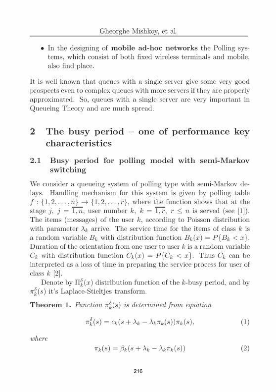
Gheorghe Mishkoy, et al.
• In the designing of mobile ad-hoc networks the Polling sys-tems, which consist of both fixed wireless terminals and mobile,also find place.
It is well known that queues with a single server give some very goodprospects even to complex queues with more servers if they are properlyapproximated. So, queues with a single server are very important inQueueing Theory and are much spread.
2 The busy period – one of performance key
characteristics
2.1 Busy period for polling model with semi-Markov
switching
We consider a queueing system of polling type with semi-Markov de-lays. Handling mechanism for this system is given by polling tablef : 1, 2, . . . , n → 1, 2, . . . , r, where the function shows that at thestage j, j = 1, n, user number k, k = 1, r, r ≤ n is served (see [1]).The items (messages) of the user k, according to Poisson distributionwith parameter λk arrive. The service time for the items of class k isa random variable Bk with distribution function Bk(x) = PBk < x.Duration of the orientation from one user to user k is a random variableCk with distribution function Ck(x) = PCk < x. Thus Ck can beinterpreted as a loss of time in preparing the service process for user ofclass k [2].
Denote by Πδ
k(x) distribution function of the k-busy period, and by
πδ
k(s) it’s Laplace-Stieltjes transform.
Theorem 1. Function πδ
k(s) is determined from equation
πδ
k(s) = ck(s+ λk − λkπk(s))πk(s), (1)
where
πk(s) = βk(s+ λk − λkπk(s)) (2)
216

Modeling of busy period in polling models with . . .
and with ck(s) and βk(s) denoting the Laplace-Stieltjes transforms of
distribution functions Ck(x) and Bk(x).Denote by PB
k
(x), PCk
(x) and P0(x) the probabilities that at in-stant x the system is busy by service of k -messages, switching to k -messages and system is free, respectively.
Theorem 2. The Laplace-Stieltjes transforms of PBk
(x), PCk
(x) and
P0(x) are determined from
pBk
(s) =λk[1− πk(s)]
s[s+ λk − λkπδ
k(s)]
, (3)
pCk
(s) =λk[1− ck(s)]
s[s+ λk − λkπδ
k(s)]
, (4)
p0(s) =1
s− [pB
k
(s) + pCk
(s)]), (5)
where πδ
k(s) and πk(s) are determined from (1) and (2).
2.2 Busy period for polling model with DD priority dis-
cipline
Let’s consider a queueing system Mr|Gr|1|∞ with DD (DiscretionaryDiscipline) priority: if the service time of ak–request is less than setvalue θk, (k = 2, . . . , r), then the arrived request with priority higherthan k (σk−1–request) achieves absolute priority, otherwise – relative.The durations of service ak–requests are independent random variablesBk with distribution function Bk(x), (k = 1, . . . , r). The durationsof switching (→ i) are random variables Ci with distribution functionCi(x), (i = 1, . . . , r). The variables Bk and Ci are independent. Anarbitrary switching (→ k) also may be interrupted by arriving σk−1-request.
We’ll introduce notations following [3, 4]. We’ll denote by Π(x),
Πk(x), Πkk(x), Hk(x), Π(n)
kk(x), Nk(x), Πk(x), Πkk(x) the distri-
bution function of busy period, k–period, kk–period, k–service cy-cle, kkn–period, k–cycle of switching, Πk–period, Πkk–period and by
217

Gheorghe Mishkoy, et al.
π(s) . . . πkk(s) – their Laplace-Stieltjes transforms (the definition ofthese see [4]). Let’s consider also σk = a1 + · · · + ak, where ak –the parameter of Poisson flow of k–th priority.
Theorem 3. For all schemes
σkπk(s) = σk−1πk−1(s+ ak − akπkk(s)) + akπkk(s), (6)
πkk(s) = hk(s+ ak − akπkk(s)), (7)
σkπk(s) = σk−1πk−1(s + ak) + σk−1πk−1(s+ ak[1− πkk(s)])−
−πk−1(s+ ak)νk(s+ ak[1− πkk(s)]) + akπkk(s), (8)
πkk(s) = νk(s+ ak[1− πkk(s)])πkk(s), (9)
where hk(s+ ak − akπkk(s)) and νk(s+ ak − akπkk(s)), for each of the
schemes I.J, are determined from certain relations respectively [4], for
s = s+ ak − akπkk(s).The analytical results formulated above, although they are of inter-
est from fundamental theoretical point of view, are quite complicatedfor numerical modelling. Indeed, for example, πk(s) given by the The-orem 3, occurs in most of the performance characteristics. But fordetermining this function it is necessary to solve the functional equa-tion (7), which does not have the exact analytical solution, but whicheffectively can be solved numerically [3, 5]. As an example, we willpresent same results of elaborated numerical algorithms of successiveapproximations for determining πk(s), νk(s) and hk(s).
3 Numerical example
Example 1 It is considered a generalized queueing system with DD
priority, for the scheme 1.2 (”repeat”, ”resume”), which is formed from
k queues, k = 1, 10. The requests arrive in the queues according to
Poisson flow with the parameters ak = 0.2, 0.1, 0.9, 0.6, 0.8, 0.2, 0.1, 0.30.2, 0.9for each queue Lk, k = 1, 2, ..., 10. The service time of requests
218

Modeling of busy period in polling models with . . .
of class k is a random variable with Erlang distribution function Bk(x),with the parameters bk = 0.1, 0.2, 0.3, 0.4, 0.5, 0.2, 0.3, 0.2, 0.1, 0.1,pk = 0.5, 0.2, 8, 0.4, 4, 0.1, 0.3, 0.5, 0.9, 0.23 and the switching time
from a queue to k queue, it is considered a random variable with
Exponential distribution function Ck(x), with the parameters ck =0.4, 0.9, 0.6, 0.9, 0.1, 0.2, 0.2, 0.1, 0.9, 0.7. The set value θk = 0.4,s = 0.5, ε = 10−5.
Table 1. Numerical results of k-busy period and auxiliary characteris-tics for DD priority, ”repeat”, ”resume” discipline
k hk(s) νk(s) πk(s)
1 0.778370 0.642857 0.489282
2 1.918259e-4 0.521253 0.025329
3 0.537282 0.378999 0.075940
4 8.396915e-4 0.000000 0.135735
5 0.837261 0.000000 0.292063
6 0.522701 0.444444 0.140271
7 0.534522 0.019607 0.007274
8 0.138574 0.530092 0.025610
9 0.576717 0.414889 0.117760
10 0.127903 0.127903 0.058166
4 Conclusion
As it is mentioned above, the busy period is present in the analyticalexpressions for most of the performance characteristics. On the otherhand, it is known that functional equations by which this characteristicis expressed have no analytical solution, so the busy period cannot befound exactly. But it can be determined with the required accuracy, ap-
219

Gheorghe Mishkoy, et al.
plying numerical methods and developing calculation algorithms. Thisis achieved, and this makes it possible also to model other performancecharacteristics in the body for which the busy period is found.
References
[1] V.M. Vishnevsky, O.V. Semenova. Polling Systems: The the-
ory and applications in the broadband wireless networks. Moscow,Texnocfera, 2007 (in Russian).
[2] V.V. Rycov, Gh.K. Mishkoy. A new approach for analysis of
polling systems. Proceedings of the International Conference onControl Problems, Moscow, 2009, pp. 1749–1758.
[3] Gh. K. Mishkoy. Generalized Priority Systems. Chisinau, Acad. ofSc. of Moldova, Stiinta, 2009 (in Russian).
[4] Gh.K. Mishkoy, L. Mitev. Performance characteristics for DD
priority discipline with semi-Markov switching. Distributed Com-puter and Communication Networks, Springer, 2014, pp. 204–218.
[5] Gh.K. Mishkoy. Priority systems with orientation. Analytical and
numerical results. Analytical and Computational Methods inProbability Theory, Springer, 2017, pp. 109–120.
Gheorghe Mishkoy1, Lilia Mitev2
1V. Andrunachievici Institute of Mathematics and Computer Science,Free International University of MoldovaE–mail: [email protected]
2V. Andrunachievici Institute of Mathematics and Computer Science,Free International University of MoldovaE–mail: [email protected]
220

Proceedings of the Fifth Conference of Mathematical Society of Moldova
IMCS-55, September 28 - October 1, 2019, Chisinau, Republic of Moldova
Solving the non-linear 4-index
transportation problem
Tatiana Pas,a, Valeriu Ungureanu
Abstract
We formulate the 4-index transportation problem with theconcave piecewise cost function. We describe an algorithm forsolving the non-linear problem and bring a practical example todescribe the implementation of the algorithm.
Keywords: transportation problem, non-linear program-ming.
1 Introduction
The 4-index transportation problem (4ITP) is a mathematical modelthat describes very well the activity of an enterprise, which attractsattention of researchers, because the problem assumes that the capaci-ties of the sources, the demands of the destinations to be supplied, thetypes and quantities of products and the types and capacities of thetransports are known.
The problem is a part of the 4ITP group which was studied by R.Zitouni, who proposes an original algorithm [1] and compares it withother methods [2]. A modification of the classical algorithm was de-scribed by A. Djamel et. al. [3]. In [4] the nonlinear 4-index transporta-tion problem (N4ITP) was formulated and an algorithm was proposedthat simplifies the problem to a linear problem for which the simplexalgorithm can be applied.
A well-known tool for solving this kind of problems is the Mathe-matica System, in which the proposed algorithm was implemented andtested.
c©2019 by Tatiana Pas,a, Valeriu Ungureanu
221

Tatiana Pas,a, et al.
2 Problem formulation
In the following, we are given:
- m sources A1, . . . , Am with the respective supply α1, . . . , αm;
- n destinations B1, . . . ,Bn with the respective demand β1, . . . , βn;
- p different types of products P1, . . . , Pp of respective quantitiesγ1, . . . , γp;
- q different types of transport T1, . . . , Tp with the respective trans-portation capacities δ1, . . . , δq.
The N4ITP needs to determine a flow that minimizes the function
F (x) =m∑
i=1
n∑
j=1
p∑
k=1
q∑
l=1
ϕijkl(xijkl), (1)
where ϕijkl(xijkl) are concave piecewise non-decreasing cost functions.
We must solve the non-linear problem:
F (x∗) = minx∈X
F (x) (2)
n∑
j=1
p∑
k=1
q∑
l=1
xijkl = αi, ∀i = 1, . . . ,m
m∑
i=1
p∑
k=1
q∑
l=1
xijkl = βj , ∀j = 1, . . . ,n
m∑
i=1
n∑
j=1
q∑
l=1
xijkl = γk, ∀k = 1, . . . ,p
m∑
i=1
n∑
j=1
p∑
k=1
xijkl = δl, ∀l = 1, . . . ,q
xijkl ≥ 0, ∀(i, j, k, l)
(3)
To respect constraints on positive values, the following variablesα1, . . . ,αm, β1, . . . ,βn, γ1, . . . ,γp and δ1, . . . ,δq must be positive.
222

Solving the non-linear 4-index transportation problem
3 Main results
The proposed genetic algorithm for solving N4ITP with concave piece-wise cost functions consists of the following steps:
Step 1. Initialization — generate an initial population of 4nmchromosomes, each described by a list of the form:
P = p(i, j), i = 1, ..., n, j = 1, ...,m‖
‖ p(1), . . . , p(p) ‖p(1), . . . , p(q) .
Step 2. De-codification — associate each chromosome with anadmissible solution. Evaluation — calculate the cost for each arc onwhich the flow is being pushed and the value of the objective functionfor each solution.
Step 3. In order to select the parent chromosomes that will partic-ipate in the creation of the next population, they are sorted in increas-ing order according to the value of the objective functions associatedwith the chromosomes and the first half will be transferred to the nextpopulation and selected as parent chromosomes.
Step 4. Crossover — perform between selected pairs. The parentchromosomes are cut in the same random place. The first descendantobtains the sequences of arcs up to the cut and the order of distribu-tion of the products from the mother chromosome, the order of thetransports and the other sequences of arcs are taken from the fatherchromosome. The second descendant obtains the sequences of arcs upto the cut and the order of distribution of the products from the fatherchromosome, the order of the transports and the other sequences ofarcs are taken from the mother chromosome.
Step 5. Perform mutation at a rate ǫ and implies:- randomly the section of the chromosome is chosen, products or
transports;- for the selected section two elements are selected randomly and
swapped.Step 6. Check the stop condition — the algorithm stops after k
iterations. The solution to the problem corresponds to the chromosome
223

Tatiana Pas,a, et al.
with the minimum objective function. If the ending condition is notverified, proceed with Step 2.
4 Conclusion
The experimental results demonstrate the correctness of the describedalgorithm and if we perform a sufficient number of iterations, the op-timal solution of the problem will be obtained. The algorithm exitsbottlenecks and tends to local solutions using the operations of selec-tion, crossing and mutation.
References
[1] R. Zitouni, A. Keraghel, D. Benterki. Elaboration and Implemen-
tation of an Algorithm Solving a Capacitated Four-Index Trans-
portation Problem. AMS, vol. 1(53), 2007, pp. 2643–2657.
[2] R. Zitouni, M. Achache. A numerical comparison between two ex-
act simplicial methods for solving a capacited 4-index transporta-
tion problem. JNAA, vol. 46(2), 2017, pp. 181–192.
[3] A. Djamel, N. Amel, L.T. Hoai, Z. Ahmed. A modified clasical al-
gorithm ALPT4C for solving a capacitated four-index transporta-
tion problem. ACTA MV, vol. 37(3), 2012, pp. 379–390.
[4] T. Pas,a. Multi-index transport problem with non-linear cost
functios. ROMAI J., vol. 14, no.2, 2018, pp. 129-–137,https://rj.romai.ro/ (to appear).
Tatiana Pas,a1, Valeriu Ungureanu2
1Moldova State University,Chis
,inau, Republic of Moldova
E–mail: [email protected]
2Moldova State University,Chis
,inau, Republic of Moldova
E–mail: [email protected]
224

Proceedings of the Fifth Conference of Mathematical Society of Moldova
IMCS-55, September 28 - October 1, 2019, Chisinau, Republic of Moldova
On determining coefficients matrices for
transmission line equations
Vladimir Patiuc, Galina Rıbacova
Abstract
The numerical technique for computing the matrix of poten-tial coefficients for multi-wire electrical lines is proposed. Theobtained results are compared with existing methods for calcu-lating these coefficients. The applicability limits of the proposednumerical method are studied depending on the initial parame-ters of a multi-wire power line.
Keywords: transmission line, finite volume method, poten-tial coefficients matrix.
1 Mathematical model
When studying electromagnetic processes in a multi-wire long powerlines, the telegrapher’s equations (or just telegraph equations) are of-ten used [1] and [2]. The telegraph equations are a pair of coupled,linear differential equations that describe the voltage and current onan electrical transmission line with distance and time. These equationswith respect to voltage vector u(x, t) and current vector i(x, t) havethe form
L∂i
∂t+
∂u
∂x+Ri = 0 (1)
C∂u
∂t+
∂i
∂x+Gu = 0 (2)
c©2019 by Vladimir Patiuc, Galina Rıbacova
225

Vladimir Patiuc, Galina Rıbacova
In an n-wire line the vector functions u(x, t) and i(x, t) have n
components each, but L, C , R, G in Eqs. (1) and (2) are symmetri-cal matrices (n× n) of per-unit-length inductances, capacitances, wireresistances and conductivities of insulation.
When solving a problem for telegraph equations Eqs. (1) and (2),it is usually assumed that the matrices L, C , R, G are known. Mostoften, the values of the coefficients of these matrices are taken fromreference books or specialty literature, where these values obtainedexperimentally are represented. Here we present an algorithm thatallows computing the potential coefficients matrix numerically.
The transmission line equations contain the matrix of the coef-ficients of electrostatic induction which allows expressing the chargevector through the vector of potentials in each conductor. The methodfor calculating the exact values of its coefficients is proposed in [1].For this purpose it is necessary to solve n (number of wires) Dirich-let problems with known boundary conditions. At the same time itis proposed numerical method for calculating the potential coefficientsmatrix, which allows to express the vector of potentials through thecharge vector in each conductor. In order to obtain the elements of thismatrix we obtain the problem that differs from the classical Dirichletproblem for the Laplace equation. The difference consists in replacingthe Dirichlet condition by some special boundary condition, which con-tains integrals over the boundary of the domain from the values of theunknown function. Such problems are called problems with nonlocalboundary conditions.
2 Potential coefficients matrix for two-wire
power line
The detailed description and the theoretical foundation of the formu-lated problem with nonlocal boundary conditions are presented in [4].The existence and uniqueness of the solution of such a problem areproved in [4] as well. In order to solve numerically the foregoing prob-lem we propose to apply the ideas of the finite volume method. So, the
226

On determining coefficients matrices for transmission line equations
corresponding algorithm has been developed and implemented usingMatlab numerical computing environment.
At the same time, elements of the potential coefficients matrix un-der certain assumptions can be calculated by the formulas given in [3].To obtain these formulas, one wire is selected and the presence of anelectric charge is assumed only on it, but on all other wires the chargeis considered zero. It is assumed also that the field of the charged wirewill be the same as the field of a single wire stretched above the earth(since the distortion of the field due to the existence of other wirescan be neglected due to the smallness of their cross sections and theabsence of the electrical charges on them).
The calculations performed by the proposed numerical algorithmfor the test problem are in good agreement with the data obtainedusing the technique described in [3], which allows us to recommendthe proposed method for calculating the parameters of objects withcomplex geometry.
On the other hand, the calculations demonstrated that for wires ar-rangement, that is used in practice, the values of capacitive coefficientscan be calculated with sufficient accuracy using simple approximateformulas for potential coefficients. To confirm this statement we havesolved numerically several problems for two-wire line with distinct ini-tial data. So, consider the problem for two wires with the centers atthe points (−d/2,H), (d/2,H). Here d, R, H represent the distancebetween wires, the radius of each wire and the height of their loca-tion above the earth, respectively. We have chosen for the study thefollowing main parameters: the ratio between the radius of the wiresand the distance between their centers, the ratio between the heightof wire location above the earth and the radius. All the obtained nu-merical data have been compared with the corresponding calculationsperformed in accordance with [3]. As an example, let us present the re-sults of calculating the potential coefficients matrix α according to theproposed method and the matrix αanal obtained by the formulas from[3]. Considering the case when d = 0.036, R = 0.012, H = 0.024 ord/R = 3,H/R = 2 (i.e. the values of the height of wires location H, of
227

Vladimir Patiuc, Galina Rıbacova
the distance between their centers d and of the radii R are comparable),we obtain:
α =
(
2.284 0.8030.803 2.284
)
· 10101
F, (3)
αanal =
(
2.367 0.9180.918 2.367
)
· 10101
F. (4)
In order to prove the convergence of the proposed method the numericalexperiments have been fulfilled using grid thickening.
References
[1] W.T. Weeks. Multiconductor Transmission-line Theory in the
TEM Approximation. IBM Journal of Research and Development,vol. 16, no. 6, 1972, pp. 604–611.
[2] P. Clayton. Analysis of multiconductor transmission lines. 2nd Ed.Wiley-IEEE Press, 2007, 780 p.
[3] K.S. Demirchyan, N. V. Korovkin, V.L. Chechurin. Theoreticalfoundations of electrical engineering. vol. 3, SPb:Piter, 2004, 364p. (in Russian).
[4] V. Patiuc. Numerical Method for Determining Potential Coeffi-
cients Matrix for Multiconductor Transmission Line. Problems ofregional energetics, vol. 3(38), 2018, pp. 28–35.
Vladimir Patiuc1, Galina Rıbacova2
1Department of Mathematics/Moldova State UniversityE–mail: [email protected]
2Department of Mathematics/Moldova State UniversityE–mail: [email protected]
228

Proceedings of the Fifth Conference of Mathematical Society of Moldova
IMCS-55, September 28 - October 1, 2019, Chisinau, Republic of Moldova
Modeling of the formation of protostellar cores
in the clouds-clouds collision
Boris Rybakin, Sergey Moiseenko, Grigore Secrieru
Abstract
The paper presents the results of numerical modeling of theprocess of collision of two molecular clouds (MC).
Keywords: CFD, simulation, cloud-cloud collision (CCC),KH instabilities.
1 Introduction
The paper presents the results of mathematical modeling, which al-lows one to study the results of turbulization of the MC substance andthe effect of instabilities on the resulting dense clumps and filamentstructures. This process is accompanied by Kelvin-Helmholtz (KN) in-stability and a violation of the gas density above the perturbed surfacelayers of the clouds.
The calculation results showed that the mutual collision of the MCleads to the formation of a superdense region on the surface of thecollision, in which ever denser gas clumps are constantly formed. Thesedense clumps (lumps) are gravitationally unstable according to Jeansand are the precursors of new stars and star clusters [1]. A thermalpressure in the MC of 10–20 K is not enough to prevent gravitationalcollapse.
2 The mathematical model and simulations
Three-dimensional motion of the gaseous medium arising upon the col-lision of molecular clouds will be described by the system of Eulerequations written in a conservative form.
229

Boris Rybakin, Sergey Moiseenko, Grigore Secrieru
Here, ρ - density, u = (u, v, w) is the velocity vector, e is the energy,p is the pressure. The ongoing processes will be considered adiabatic,with adiabatic index γ = 5/3. For the solution of the basic equationsthe TVD scheme of second order of accuracy was applied. Numericalsimulations of different cases of MS collisions were carried out: a frontalcollision with the mutual penetration of two molecular clouds of aninitially spherical shape, moving in the opposite direction at differentspeeds, and a moving cloud collision. The main physical parametersand initial assumptions for modeling CCC are given in [2].
3 Numerical results
The calculation results showed that the mutual collision of the MCleads to the formation of a superdense region on the surface of thecollision, in which ever denser gas clots are constantly formed. Thesedense clumps (lumps) are gravitationally unstable according to Jeansand are the precursors of new stars and star clusters [1]. Figure 1 shows
Figure 1. Stage of passage by cloud MC1 of cloud MC2 and the for-mation of superdense clumps
how a core is formed from fragmented gas condensations. An image
c©2019 by Boris Rybakin, Sergey Moiseenko, Grigore Secrieru
230

Formation of protostellar cores in the clouds-clouds collision
is given normalized to the maximum value of the isosurface abs(gradX ) – a value characterizing a sharply variable rate of change of gasdensity. The distribution of fragmented gas condensations correspondsto a contrast X of the order 8000. The analysis shows that the con-densations in the form of “clumps” are breaking up into fragments,distributed sporadically along the arcs of concentric circles, with theirradius dynamically changing.
Figure 2. Illustration of pulsation changes in the core for the contrastratio X = 500/100
Figure 2 shows the temporal evolution of the field of rapidly chang-ing density contrast in the core (red color) and in the shell (greencolor). The maximum density contrast X in a collision at relativelylow speeds increases by two orders of magnitude compared to the ini-tial contrast X = 500. A change in the density, shape, and position ofthe contact surface leads to the appearance of vibrations that arise onthe mid lines (equators) of the MS, and the appearance of vibrations inthe interstellar environment. With further interaction of the MC, theshock-compressed lenticular layer forms superdense regions (clumps).
4 Conclusion
The process of formation of filaments, superdense, gravitationally con-nected objects and the destruction of molecular clouds was studied.The formation of Kelvin-Helmholtz and Richtmeyer-Meshkov instabil-ities is studied. Supersonic turbulence was developed, which can lead tovibrations, the formation of filaments and superdense regions (clumps),
231

Boris Rybakin, Sergey Moiseenko, Grigore Secrieru
as well as the formation of gravitationally bound regions and the pos-sible appearance of new stars.
Acknowledgments. The present investigation was supported byPresidium RAS.
References
[1] B. Wu, J. C. Tan, F. Nakamura, S. Van Loo, D. Christie, andD. Collins. GMC Collisions as Triggers of Star Formation. II.
3D Turbulent, Magnetized Simulations. The Astrophysical Jour-nal, 835:137, 2017 February 1.
[2] B. Rybakin, V. Goryachev. Parallel algorithms for Astrophysics
Problems, Lobachevskii Journal of Mathematics, vol. 39, no.4, pp.562–570, 2018.
[3] R.I. Klein. Star formation with 3-D adaptive mesh refinement: the
collapse and fragmentation of molecular clouds, J. Comp. Appl.Mat., vol. 109, pp.123–152, 1999.
Boris Rybakin1, Sergey Moisenko2, Grigore Secrieru3
1Prof./MSU, Faculty of Mechanics and Mathematics; SRISA RAS, Moscow, RussiaE–mail: [email protected]
2Dr.Habil./Space Research Institute RAS. Moscow, RussiaE–mail: [email protected]
2PhD/Vladimir Andrunachievici Institute of Mathematics and Computer Science,Chisinau, MoldovaE–mail: [email protected]
232

Proceedings of the Fifth Conference of Mathematical Society of Moldova
IMCS-55, September 28 - October 1, 2019, Chisinau, Republic of Moldova
Computer simulation of impulsive loading on
buried projectile
Boris Rybakin, Grigore Secrieru, Elena Gutuleac
Abstract
The purpose of the paper is mathematical modelling and anal-ysis of impulsive loading on buried projectile. Numerical calcu-lations for various values of ground parameters, initial pressureand projectile shell material have carried out.
Keywords: elastic-plastic model, projectile, detonation wave.
1 Introduction
Currently Moldova has ammunition depots, which pose a serious dangerto nearby civilian objects and the population in the event of strongimpact or earthquake. Field experiments are dangerous and expensive,whereas the results of computer simulation can be of practical use toensure the safety of military facilities. Also the numerical calculationscan be used in different industrial sectors with scheduled blasting.
2 The mathematical model
For the detailed study of the processes, occurring in the ground andburied structure, the model of elastic plastic body has chosen. Thismathematical model includes main equations, expressing the laws ofpreservation of mass, the quantity of motion and energy in case of twospatial variables in the Lagrange coordinate system.
The governing system is complemented by the Prandtl-Reuss equa-tions for the elastic plastic condition with von Mises yield criterion.
c©2019 by Boris Rybakin, Grigore Secrieru, Elena Gutuleac
233

Boris Rybakin, Grigore Secrieru, Elena Gutuleac
It closes with the equation of state relating state variables such aspressure, volume, internal energy [1]. After the analysis of the knownequations of state the following equations have been selected:
• Mie-Gruneisen equation for modelling the material projectile [2];
• the mathematical model based on experimental data, publishedby Lyakhov G. and Pokrovsky G. for the description of water-saturated ground [3];
• Theta law for explosives in the solid phase and Landau-Stanyuko-vich polytropic rule for detonation products.
3 Numerical method
The numerical solution is based on the finite difference method. Atthe initial moment of time the computational domain is a rectangu-lar in plane or cylindrical coordinate system. The mathematical baseof numerical calculations is homogeneous finite-difference based on themodified Wilkins scheme [2], has the second order of accuracy in spaceand time. A modification of the Wilkins method consists in the possi-bility of creating a complex computational domain, where:
• construction may have several layers made of various materials;
• the construction may be filled with liquid, explosive or other sub-stance;
• the construction may be surrounded by ground, liquid or othersubstance.
4 Numerical results
The buried projectile is modelled as a steel structure filled with explo-sive and having two fuses (in the center – fuse 2, in the end – fuse 1),
234

Computer simulation of impulsive loading on buried projectile
whose sensitivity to detonation is 3% higher of the filler explosive sub-stance. The projectile is surrounded by saturated ground environment.Impulsive loading is modelled in two ways: with pressure function as aboundary condition on the left boundary of the computational domain;with explosion of shellless charge at time t = 0 µs.
Figure 1. Pressure distribution in control points
Fig.1 shows pressure distribution at the control points located inboth fuses. The shock wave reaches the first fuse (fuse 1) and secondfuse (fuse 2) almost instantly. The critical pressure in the first fuse isexceeded and initiates detonation there. The second fuse don’t deto-nate in the same time. The detonation wave propagates through theprojectile filler, reaching the second fuse at time t = 121 µs. For thegiven initial and boundary conditions the relationships between groundparameters, initial pressure values and the character of projectile det-onation have found. Also the critical pressure for initiating detonationhas determined.
5 Conclusion
Computer simulation allows conducting numerical experiments in awide range of parameters, tracking in real time all the stages of the
235

Boris Rybakin, Grigore Secrieru, Elena Gutuleac
detonation process inside the projectile, followed by deformation of theprojectile shell. Also of interest is the mathematical modelling of theinitiation of an explosion inside the explosive shell, followed by thepenetration of a cumulative jet into a combined obstacle [4].
Acknowledgments. Moldovan Institutional Projects 15.817.02.01A,15.817.02.02A and grant No 18-07-01303A from the Russian Founda-tion for Basic Research have supported part of the research for thispaper.
References
[1] B. Rybakin. Computer Modeling of Dynamic Processes, CSJM,vol.8, no. 2(23), 2000, pp. 150–180.
[2] M.L. Wilkins. Modelling the behaviour of materials, Proceedingof International Conference. vol.2, London, New York, 1984, pp.243–277.
[3] G.M. Lyakhov, G.I. Pokrovskii. Blast Waves in Soils [in Russian],Gosgortekhizdat, 1962, p. 105.
[4] B.P. Rybakin, N.N. Smirnov, V.D. Goryachev, M.N. Kravchenko,L.I. Stamov. Computer simulation of the formation exposing pro-
cess using cumulative shaped charge [in Russian], Bulletin of Cy-bernetics, no. 3(31), 2018, pp. 1–10.
Boris Rybakin1, Grigore Secrieru2, Elena Gutuleac3
1Prof./Lomonosov Moscow State University, Faculty of Mechanics and Mathemat-ics; SRISA RAS, Moscow, RussiaE–mail: [email protected]
2PhD/Vladimir Andrunachievici Institute of Mathematics and Computer Science,Chisinau, MoldovaE–mail: [email protected]
3PhD/Vladimir Andrunachievici Institute of Mathematics and Computer Science,Chisinau, MoldovaE–mail: [email protected]
236

Proceedings of the Fifth Conference of Mathematical Society of Moldova
IMCS-55, September 28 - October 1, 2019, Chisinau, Republic of Moldova
Chebyshev parameters applied to modeling
nonlinear processes in semiconductor devices
Galina Sprincean
Abstract
The problem investigated relates to the use of Chebyshev pa-rameters for numerical modeling of nonlinear processes in semi-conductor devices. The mathematical model of the problem rep-resents a system of nonlinear differential equations in the un-knowns ϕ – electrostatic potential, ϕn, ϕp – quasi Fermy’s levelsfor electrons and holes, respectively. The problem is further com-plicated by the fact that the border conditions are of two types:the Dirichlet conditions and the Neumman conditions, which acton different portions of the border. The subproblems that weresolved in this research are: discretization of nonlinear differentialequations, separation of obtained algebraic systems and lineariza-tion of system equations. The obtained linear algebraic systemshave symmetric, positively defined and rare (five diagonal) ma-trices. To solve them many iterative methods can be applied, inthis research the Chebyshev two-layer parameter method will beapplied.
Keywords: Nonlinear processes, semiconductor devices,doping, discrediting, linearization, Cebyshev parameters.
1 Introduction
Let’s consider a semiconductor diode model (fig.1). The diode consistsof two regions with different types of doping: the hole zone (p-typezone), with a dominant hole concentration and the electron zone (n-type), with a dominant electron concentration. The anode electrode
c©2019 by Galina Sprincean
237

Galina Sprincean
is connected to the p-type region and the cathode is connected to then-type region. The impurities, added to the semiconductor material,made of silicon, determine the type of conductivity of each zone. Insemiconductor physics the concentration of impurities is noted withN. The function N(x1, x2) = N
+
D(x1, x2)−N
−
D(x1, x2)m
−3 defines the
profile of impurities and is expressed by the concentration of ionizeddonors and acceptors, noted by N
+
DandN
+
D, respectively. The negative
value of the impurity concentration is determined by the dominance ofboron acceptor atoms (p-type semiconductor), and a positive valueis determined by the dominance of phosphorus donor atoms (n-typesemiconductor).
2 Mathematical formulation of the problem
based on the drift diffusion model (DDM)
The problem solving area is a rectangular surface Ω = (x1, x2) : 0 ≤ x1 ≤
lx1
, 0 ≤ x2 ≤ lx2), (fig. 1). With ΓD note the border of this field, marked with
a thick line and the words ”cathode / anode”. We define on this part of theborder the values of unknown functions, thus obtaining Dirichlet’s conditions.On the remaining portion of the border, denoted by ΓN , we equate the values
238

Chebyshev parameters applied to modeling nonlinear processes in . . .
of the partial derivatives of the unknown functions with zero (the normal fluxat the border), thus obtaining Neumann’s conditions. Suppose that∂Ω = ΓD
⋃
ΓN , ΓD
⋂
ΓN = ∅.
∇· (ǫ∇ϕ) = q(p−n+N) (Poisson′s equation) (1.1)
−∇·(Jn) = −q(RSRH+RAUG) (The continuity equation for electrons) (1.2)∇· (Jp) = −q(RSRH +RAUG) (The continuity equation for holes) (1.3)Jn = −qnµn∇ϕn (Current density for electrons) (1.4)Jp = −qpµp∇ϕp (Current density for holes) (1.5)ϕn = ϕ− ϕT · ln(n/ni) (Cuasi Fermi
′s level for electrons) (1.6)
ϕp = ϕ+ ϕT · ln(p/ni) (Cuasi Fermi′s level for holes) (1.7)
Here ǫ = ǫrǫ0 – absolute permittivity (dielectric constant); ǫr – relative per-mittivity (ǫr = 11, 8); ǫ0 – electric constant (ǫ0 = 8, 854187817∗10−12
F ·m−1);q – positive electron charge (q = 1, 60217656510−19C); N – concentration ofimpurities; Jn si Jp – density of electron currents and holes, respectively;RSRH , RAUG – speed of recombination Shockley-Hall.
Border conditions
Consider that the cathode is grounded (Vc = 0) and an external voltage isapplied to the anode Va > 0. Then on the border ΓD, i.e. at the anode andcathode, functions ϕ, n, p satisfy relations:ϕ(x) = Va + ϕT · ln((N +
√
N2 + 4n2
i)/(2ni);
n(x) = (N +√
N2 + 4n2
i)/2; p(x) = (−N +
√
N2 + 4n2
i/2, x ∈ ΓD.
(1.8)On the portion ΓN the border conditions are in the form of Neumann’s con-ditions: ~n · ∇ϕ = ∂ϕ/∂n = 0;~n · Jn = 0;~n · Jp = 0, ~x ∈ ΓN , (1.9) where thepoint means the scalar product of the vectors.
Initial conditions
In the absence of external voltage on the anode (Va = 0) the solution of theproblem on the whole surface Ω is (1.8). This solution can be used as aninitial approximation of the sistem solution (1.1)–(1.7) at its resolution bythe iterative method, with the gradual increase of the external voltage on theanode Va.
3 Solving the problem in two-dimensional space
Based on the chosen network of nodes, following the discredit of the differen-tial equations of the system (1.1) – (1.3) three algebraic systems of nonlinear
239

Galina Sprincean
equations are obtained. The boundary conditions are also discredited by fi-nite differences, on the chosen network, and by solving the algebraic systemsobtained we establish the initial values of the unknown functions, noted byϕ0, ϕ
0
n, ϕ
0
pon Ωh. For the equation (1.1), after discrediting on the chosen
network, we obtain the following linear algebraic system, the number of equa-tions whose number coincides with the number of internal nodes (NNxMM):
2ǫ( 1
h2
x1
+ 1
h2
x1
)ϕ(k+1)
ij− ǫ
h2
x1
(ϕ(k+1)
i+1,j+ϕ
(k+1)
i−1,j)− 1
h2
x1
(ϕ(k+1)
i,j+1+ϕ
(k+1)
i,j−1) = q(p
(k)
ij−
n(k)
ij+N
(k)
ij, pe Ωh,
We apply the Chebyshev parameter method for the two-level scheme:
Bϕ
(k+1)
−ϕ(k)
τk+1
+Aϕ(k) = f
(k), B = E.
τk+1 = τ0
1+ρ0tk, k = 1, 2, . . . , n, n0(error) =
ln(2/error)
ln(1/ρ1)
, n = [n0] + 1
τ0 = 2/(λmin(A)+λmax(A)), ρ0 = (1−√ξ)/(1+
√ξ), ξ = λmin(A)/λmax(A)),
tk = (2k−1)n
2n, k = 0, 1, . . . , n − 1, λmin(A), λmax(A)– the eigenvalues of the
algebraic system operator.Because determining our own values, in some cases, is a rather complex prob-lem, in practice we have done so:a) We estimate the maximum eigenvalue, which of the observed ones is aconstant value and depends only on the domain of definition of unknownfunctions.:λmax(A) = 4/(h2
x1
)cos2((πhx1
)/(2lx1
)) + 4/(h2
x2
))cos2((πhx2
)/(2lx2
))b) We are looking for it’s minimum value in the form:
λmin(A) = λmin(A)(teoretic) ∗ α = ǫ ∗ ( π
2
(l2x1
+ π2
l2x2
) ∗ α
The parameter α = 0.4 has been determined experimentally, so that thenumber of iterations coincides with the number of iterations theoretically n,for the chosen network. If we note by ℵn the set of roots of the Cheby-
shev polynomials : ℵn = −cos(2i−1)
2n∗ π, i = 1, 2, . . . , n, then the itera-
tive parameters of Cebashev will be calculated according to the formula:τk = τ0/(1 + ρ0µk), µk ∈ ℵn, k = 1, 2, . . . , n. The successiveness of the roots,based on which the parameters of Cebashev are calculated, is of great impor-tance. The speed of convergence depends on the successiveness of the roots,and in the cases of the successive successions, phenomena such as the ”down-time” of the machine may occur, as a result of the increase of the intermediateiterations, or the loss of the accuracy of the solution, due to the accumulationof the error following the rounding. A way to construct optimal consecutiveof the parameters of the method θn is:Whether n ∈ N
∗ – number of iterations required.Step 1: We represent this number as the sum of the powers under 2 as follows:
240

Chebyshev parameters applied to modeling nonlinear processes in . . .
n = 2k1 + 2k2 + · · ·+ 2ks , kj ≤ kj−1 − 1, j = 2, 3, . . . , s.
Step 2: We calculate the following value: nj =∑
j
i=12ki−kj , j = 1, 2, . . . , sns+1 =
2n+ 1.Step 3: We build the following sets:
θnj= θ
(nj)
i= θ
(nj−1)
i, θ
(nj)
nj = nj, i = 1, 2, . . . , nj − 1. For j = 1 we choose
θ1 = 1. Then we build the crowd: θ2m = θ(2m)
2i= 4m − θ
(m)
i, θ
(2m)
2i−1=
θ(m)
i, i = 1, 2, . . . ,mfor m = nj , 2nj, 4nj, . . . , [
nj−1
4]. If [(nj − 1)/4] < nj,
then the calculations according to Step 3 are not performed and proceed tothe next step.Step 4 If j = s, then the crowd θn is built. In case of contract we
calculate m = (nj+1 − 1)/2 and we build the crowd: θ2m = θ(2m)
2i=
4m+ 2− θ(m)
i, θ
(2m)
2i−1= θ
(m)
i, i = 1, 2, . . . ,m.
Step 5 Then j increases its value by one unit and the calculations start againwith step 2. Finally, when the set θn will be constructed, and based on thisset, the set of parameters Cebashev ℵn will be ordered, thus we obtain the
optimum consecutivity of Chebyshev’s parameters ℵ(optimal)
n .
4 Conclusion
The numerical solution for algebraic systems was obtained by discretizing thenonlinear differential equations (1.1)–(1.3). The case of dynamic equilibriumV = 0 is represented in figure 2. Figure 3 represents the surfaces of unknownfunctions ϕ, ϕn and ϕp, when applying to anode, from outside, the voltageVa = 0.1V and with a concentration of impurities N ≈ 1018. Figure 4 illus-trates the distribution of functions ϕ, ϕn and ϕp, when applying to anode,from outside, the voltage Va = 0.2V and with a concentration of impuritiesN ≈ 1018.
References
[1] W.H.A. Schilders and E.J.W. ter Maten. Numerical Methods in Electro-
magnetics. Special Volume of HANDBOOK OF NUMERICAL ANAL-YSIS, Vol. XIII. ELSEVIER, Amsterdam, 2005, 912 p.
[2] A.A. Samarschii, E.S. Nicolaev. Methods for solving grid equations.
Moscow, 1978, pp. 269–283 p.
241

Galina Sprincean
Galina Sprincean
Moldova State University, str. Alexe Mateevici, 60 Chisinau, MD-2009, Republic ofMoldovaE–mail: [email protected]
242

Proceedings of the Fifth Conference of Mathematical Society of Moldova
IMCS-55, September 28 - October 1, 2019, Chisinau, Republic of Moldova
Investigation of Some Cryptographic Properties
of the 8x8 S-boxes Created by Quasigroups
Aleksandra Stojanova, Dusan Bikov,
Aleksandra Mileva, Yunqing Xu
Abstract
We investigate several cryptographic properties in 8-bit S-boxes obtained by quasigroups of order 4 and 16 by differentmethods. The best produced S-boxes so far are regular and havealgebraic degree 7, nonlinearity 98 (linearity 60), differential uni-formity 8, and autocorrelation 88.
Keywords: Nonlinearity, differential uniformity.
1 Introduction
The main building blocks for obtaining confusion in all modern blockciphers are so called substitution boxes, or S-boxes. Designers of blockciphers very often choose S-boxes with special cryptographic proper-ties, which means high nonlinearity (or low linearity), low differentialuniformity, high algebraic degree, low autocorrelation and regularity(balance). The well known fact is that the bijective S-boxes are alwaysregular. The AES S-box is the example of the best found 8x8 S-boxes,which is optimal with respect to most of the cryptographic properties(with algebraic degree 7, nonlinearity 112 (or linearity 32), differentialuniformity 4, and autocorrelation 32).
Let F2 denote the Galois field with two elements, and let Fn
2denote
the vector space of binary n-tuples over F2 with respect to addition⊕ and scalar multiplication. An n−ary Boolean function is a func-tion f : Fn
2→ F2. A Boolean map is a map S : Fn
2→ F
m
2, (m ≥
1). Every Boolean map S can be represented as: S(x1, . . . , xn) =
c©2019 by A. Stojanova, D. Bikov, A. Mileva, Yu. Xu
243

Aleksandra Stojanova, et al.
(f1(x1, . . . , xn), f2(x1, . . . xn), . . . , fm(x1, . . . , xn)). Each fi can be rep-resented in ANF as fi(x1, x2, . . . , xn) =
⊕
I⊆1,2,...,nαI(
∏
i∈Ixi),
where αI ∈ F2.
For all x ∈ Fn
2, the Walsh-Hadamard transform Wf : Fn
2→ R of
f is Wf (x) =∑
a∈Fn
2
(−1)f(a)⊕a·x, where Wf (x) ∈ [−2n, 2n] is known
as a spectral Walsh coefficient, while the Autocorrelation transform off is ACTf (x) =
∑
a∈Fn
2
(−1)f(a)⊕f(a⊕x), where ACTf (x) ∈ [−2n, 2n]is known as a spectral autocorrelation coefficient. The autocorrelation
(absolute indicator) of f is AC(f) = maxx∈Fn
2\0
|ACTf (x)|. The nonlinear-
ity of a Boolean function f is defined as NL(f) = 2n−1− 1
2maxx∈Fn
2
|Wf (x)|,
while the linearity of f is defined as L(f) = maxx∈Fn
2
|Wf (x)|. They are
related by the equation L(f) + 2NL(f) = 2n.
For Boolean map S we have the following definitions [2, 3]:
• Algebraic degree: deg(S) = maxi∈1,2,...,m
deg(fi)
• Nonlinearity: NL(S) = minv∈Fm
2\0
NL(v · S)
• Linarity: L(S) = maxv∈Fm
2\0
L(v · S)
• Autocorrelation: AC(S) = maxv∈Fm
2\0
AC(v · S)
• Differential uniformity: ∆(S) = maxu∈Fn
2
\0,v∈Fm2
|x ∈ Fn
2 |S(x) ⊕ S(x ⊕
u) = v|
2 Main Results
Mihajloska and Gligoroski [1] constructed optimal 4x4 S-boxes fromquasigroups of order 4, by using four e quasigroup transformations,alternating in normal and reverse mode (in a sense that they applythe string in reverse order – oe). We investigate several cryptographicproperties of the 8x8 S-boxes obtained by similar constructions withquasigroups of order 4 and 16. In some of the constructions we com-bine quasigroup transformations with the addition of 2-, 4-, or 8-bitconstants.
244

Investigation of Some Cryptographic Properties of the 8x8 S-boxes...
Method 1 – alternate use of e and oe transformations generatedby quasigroups of order 4, like in [1]. Part of the results are given inTable 1, where neoe type means that there are total of n quasigrouptransformations.
Table 1. Method 1 – part of the results
Type NL(S) L(S) ∆(S) AC(S) deg(S) No. of S
4eoe 64 128 24 256 7 192
8eoe 98 60 10 88,96,64 7 3360
10eoe 98 60 10 88 7 27392
12eoe 98 60810
9688
7≥ 714
≥ 84281
Method 2 – combination of e and oe transformations, with addi-tion of 2-bit, 4-bit or 8-bit constants (some results in Table 2).
Table 2. Method 2 – part of the results
Type NL(S) L(S) ∆(S) AC(S) deg(S) No. of S
1e add2 0 256 256 256 4 4608
1e add4 0 256 128 256 4 2816
1e add8432
248192
132164
256 761441536
1oe add8 0 256 132 256 7 6144
2e add2 oe add2 0 256 128 256 6 98304
2e add4 oe add4 64 128 96 256 6 3072
4eoe add2 64 128 24 256 7 768
4eoe add8 88 80 24 160 7 16
Method 3 – as Method 1 and 2, but with one randomly generatedshapeless quasigroup of order 16 (Fig. 1).
The best produced 8x8 S-box is obtained by 6 e quasigroup transfor-mations, alternating in normal and reverse mode, from the quasigroupof order 16, with consecutive leaders (0, 3, 5, 3, 0, 0).
References
[1] H. Mihajloska, D. Gligoroski. Construction of Optimal 4-bit S-boxes by
Quasigroups of Order 4. SECURWARE 2012, 2012.
245

Aleksandra Stojanova, et al.
Figure 1. Shapeless quasigroup of order 16.
Table 3. Method 3 – part of the results
Type NL(S) L(S) ∆(S) AC(S) deg(S) No. of S
1e add2 32 192 34 256 6 64
1e add43264
192128
3444
256 6648
1e add8 64 128 26 232-248 7 20
2e add4 oe add49698
6460
1012,14
8896-104
7100
65536
2e add8 oe 98 60 10 88 7 11
4eoe98
94-9060
68-7610-128
8896-112
7155
6eoe 98 60 888104
712
[2] K. Nyberg. Perfect nonlinear S-boxes. In: Davies, D.W. (Ed.) Eurocrypt1991. LNCS, vol. 547, pp. 378–385. Springer, 1991.
[3] K. Nyberg. S-boxes and round functions with controllable linearity and
differential uniformity. In: Preneel, B. (Ed.), FSE 1995. LNCS, vol. 1008,pp. 111–130. Springer Berlin Heidelberg, 1995.
Aleksandra Stojanova1, Dusan Bikov1, Aleksandra Mileva1, Yunqing Xu2
1University Goce Delchev in Shtip, Republic of N. MacedoniaE–mails: aleksandra.stojanova, dusan.bikov,
2Ningbo University, Peoples Republic of ChinaE–mail: [email protected]
246

Proceedings of the Fifth Conference of Mathematical Society of Moldova
IMCS-55, September 28 - October 1, 2019, Chisinau, Republic of Moldova
Four color theorem – map solver
Natasha Stojkovikj, Mirjana Kocaleva, Jordan Miovski
and Biljana Zlatanovska
Abstract
Today graph theory has grown into a significant area of math-ematical research, with applications almost everywhere (in chem-istry, operations research, ..). In this paper, the problem of mapcoloring with four colors with theory of graphs is considered. Weconsidered the map of metropolitan area of Skopje. For coloring,the software “Four color theorem – map solver” is used.
Keywords: graph, graph theory, maps, map coloring, algo-rithms.
1 Introduction
Graphs are very practical mathematical model and they are used in var-ious areas of science and everyday life. We are considering the problemof map coloring with four colors. The problem consisted of the possibil-ity of coloring the world map with only four colors, but two neighboringcountries must not be colored with the same color [1].
This problem can be considered with the theory of graphs. Graphsare very closely related to maps, as every map can be treated as a graph.A graph G(V,E) consists of a finite non-empty set V whose elementsare called nodes, vertices, or points and a finite set E of unorderedpairs of distinct nodes, i.e. links of G [4], [5], [6].
c©2019 by Natasha Stojkovikj, Mirjana Kocaleva, Jordan Miovski and
Biljana Zlatanovska
247

Natasha Stojkovikj1, et al.
2 Chromatic number on graph
A nodes coloring (or simply coloring) of a graph G, is a labelling f :V (G) → 1, 2, .... The labels are called colors, such that no twoadjacent nodes get the same color and each node gets one color. Ak - coloring of a graph G consists of k different colors and G is thencalled k - colorable. It follows from the definition that the k - coloringof a graph G(V,E) partitions the set of nodes V into k independentsets V1, V2, ..., Vk such that V = V1∪V2∪ ...∪Vk . The independent setsV1, V2, ..., Vk are called the color classes and the function f : V (G) →1, 2, ..., k such that f(v) = i, where v ∈ Vi , 1 ≤ i ≤ k, is called thecolor function [2], [3].
For map coloring, we will use the following greedy algorithm. Thealgorithm is as follows:
Algorithm 1
1. Define Graph G.
2. Sort the nodes in descending order by degrees.
3. Assign color B1 to the first node, and then to all nodes that are not neighbors to
the previous node, but are not neighbors to each other.
4. Repeat the step 2, with color B2 for the next uncolored node.
5. Repeat the step 3 while there are nodes without colors.
6. Finish.
3 Four color theorem - map solver
“Four color theorem – map solver” is a software which paints map with4-coloring algorithm. In the Skopje there will be taken the followingMunicipalities: Novo Selo, Lepenec, Bardovci, Vizbegovo, Butel, StaroSkopje, Gazi Baba, Chair, Gorce Petrov, Centar 1, Karposh, Zlocucani,Vlae, Gorce Petrov 6, Mirce Acev, Sisevo, Saraj, Gorce Petrov 3. Toestablish a relationship with the original definition of a 4-color graphcoloring algorithm, here the nodes of the graph will be the cadastralmunicipalities themselves, and the links between the nodes, in fact willbe the borders by which they are separated (Fig.1.).
Regarding the color grading algorithm in 4 colors, to paint themetropolitan area of Skopje, 4 colors are needed. The steps of the
248

Four color theorem – map solver
Figure 1. Map of the municipalities of Skopje, properly painted with 4colors.
algorithm in the concrete case are the following (Fig.1.):
Step 1: Novo Selo has 3 neighbors (Gorce p.3, Mirce A., Lepenec); Lepenec has
5 neighbors (New V., Gorce p.6, Vlae, Zlocucani, Bardovci); Bardovci has 3 neighbors
(Lepenec, Zlocucani, Vizbegovo); Vizbegovo has 4 neighbors (Bardovci, Zlocucani, Chair,
Butel); Butel has 4 neighbors (Vizbegovo, Chair, Gazi B., Staro S.); Staro Skopje has 2
neighbors (Butel, Gazi B.); Gazi Baba has 4 neighbors (Staro S., Butel, Chair, Centar 1);
Centar 1 has 3 neighbors (Karpos, Cair, Gazi B.,); Chair has 6 neighbors (Vizbegovo, Butel,
Gazi B., Centar 1, Karposh, Zlocucani); Karposh has 5 neighbors (Centar 1, Chair, Zlocu-
cani, Vlae, Gorce p.6); Zlocucani has 6 neighbors (Karposh, Chair, Vizbegovo, Bardovci,
Lepenec, Vlae); Vlae has 4 neighbors (Gorce p.6, Karposh, Zlocucani, Lepenec); Gorce
Petrov 6 has 3 neighbors (Vlae, Lepenec, Mirce A.); Mirce Acev has 4 neighbors (Gorce
p.6, New V., Gorcep.3, Sisevo); Sisevo has 3 neighbors (Mirce A., Gorce p.3, Saraj); Saraj
has 2 neighbors (Sisevo, Gorce p.3); Gorce Petrov 3 has 4 neighbors (Saraj, Sisevo, Mirce
A., New V.)
Step 2 : We sort the municipalities in descending order by the number of neighboring
municipalities they have.
Step 3 and Step 4: Chair and Zlocucani have the same number of neighbors, so we
choose one of them. Chair is painted with one color (red) and all of its non-neighboring
municipalities (Staro S., Lepenec, Gorce P.3) will be painted with the same color. After that,
we paint Zlocucani with another color (blue) and all of its non-neighboring municipalities
(Centar 1, Butel, New V., Sisevo, Gorce p.6) will be painted with the same color. Because
Lepenec is already painted, we take the next municipality Karposh, and we paint it with a
third color (green) and all of its non-neighboring municipalities (Gazi B., Vizbegovo, Saraj,
249

Natasha Stojkovikj1, et al.
Mirce A.) will be painted with the same color. Because Vizbegovo, Butel and Gazi Baba
are already colored, we take the next municipality of the list, and it is Vlae; Vlae is painted
with a fourth color (yellow) and it is only one non-neighboring, no painted municipality
and it is Bardovci, so Bardovci will be painted with the same color as Vlae. In the end, four
colors are needed for coloring the map of Skopje. Like as example of municipality Shtip, also
for this case we can find lower and upper bounds of chromatic number of the graph (Fig.
7). This graph is neither complete nor regular, so from corollary 1, we have that 3 ≤ χ(G).
From the other side, we have that ∆(G) = max2, 3, 4, 5, 6 = 6, χ(G) ≤ ∆(G) = 6 , and
χ(G) ∈ 3, 4, 5, 6. Using the Algorithm 1 we will find that chromatic number of this graph
is 4.
References
[1] Z. Pooranian, A. Harounabadi, M. Shojafar and N. Hedayat. Newhybrid algorithm for task scheduling in grid computing to decrease
missed task, World Acad Sci Eng Technol, 55, 2011, pp.924–928.
[2] E. Raty, S. Thomasson. Map coloring: Finding the number of col-
orings of maps colorable with four colors. Valkeakosken Tietotienlukio / Paivolan Kansanopisto.
[3] J. Verstraete. Map Coloring Theorems. Map Coloring Theorems,Department of Mathematics, UCSD La Jolla CA.
[4] J. A. Bondy and R.S.U. Murty. Graph theory with application.North – Holland, New York, Amsterdam, Oxford, 1976.
[5] J.A. Bondy and R.S.U. Murty. Graph theory. Springer, 2008.
[6] R.T. Jensen and B. Toft. Graph Coloring Problems. John Wileyand Sons, Inc., 1994.
Natasha Stojkovikj, Mirjana Kocaleva, Jordan Miovski, Biljana Zlatanovska
Faculty of Computer science, Goce Delcev University, Stip, R.N.MacedoniaE–mails: [email protected], [email protected],
[email protected], [email protected]
250

Proceedings of the Fifth Conference of Mathematical Society of Moldova
IMCS-55, September 28 - October 1, 2019, Chisinau, Republic of Moldova
Method for solving fuzzy fractional multi-criteria
transportation problem of “bottleneck” type
Alexandra Tkacenko
Abstract
In this work the development of an iterative fuzzy program-ming algorithm for solving fuzzy fractional multi-objective trans-portation problem of ”bottleneck” type is described. The algo-rithm is iterative for each value of optimistic parameter of costcoefficient variation. Finally, for any value of this coefficient wewill have the set of all the efficient solutions of the model, corre-sponding to the value level of time. The algorithm was tested onseveral examples and proved to be quite effective.
Keywords: fuzzy programming, fuzzy cost, fractional trans-portation problem, efficient solution.
1 Introduction
Many of economical decision problems lead to the fractional optimiza-tion models, because a lot of important characteristics of these may beevaluated really using only some ratio relations. The time-constrainingcriterion is, obviously, one of conditions so much important for ma-jor optimization problems. There are many efficient algorithms thatsolve such models with deterministic data. Since in real life often someparameters are of fuzzy type [1], in this paper the case of fuzzy costcoefficients is investigated.
c©2019 by Alexandra Tkacenko
251

Alexandra Tkacenko
2 Problem formulation
The mathematical model of the multi-criteria fractional transportationproblem of “bottleneck” type with fuzzy cost coefficients is the follow-ing:
minZ1 =
∑
m
i=1
∑
n
j=1c1
ijxij
maxi,j
tij|xij > 0minZ2 =
∑
m
i=1
∑
n
j=1c2
ijxij
maxi,j
tij|xij > 0
........
minZr =
∑
m
i=1
∑
n
j=1cr
ijxij
maxi,j
tij |xij > 0minZr+1 = max
i,j
ti,j| xi,j > 0 (1)
n∑
j=1
xij = ai, ∀i = 1,m,
m∑
i=1
xij = bj , ∀j = 1, n,
m∑
i=1
ai =
n∑
j=1
bj, xij ≥ 0 for all i and j,
where : ck
ij, k=1,2. . . r, i=1,2,. . .m, j=1,2,. . . n are costs or other
amounts of fuzzy type, tij – necessary unit transportation time fromsource i to destination j, ai – disposal at source i, bj – requirement ofdestination j, xij – amount transported from source i to destination j.
In the model there may also exist the criteria of maximum, whichhowever does not complicate it.
3 Theoretical benchmarks
For the reasons that the time characteristic for the model (1) is discrete,it follows that the set of efficient solutions for every level of its allowabletime coincides with the set of efficient solutions for multi-criteria linearmodel, including separate “bottleneck” criterion [2]. Since the costcoefficients of transportation multi-criteria models have real practicalsignificance such as unit prices, unit costs and many other, all of them
252

Method for solving fuzzy fractional multi-criteria transportation ...
are interconnected with the same parameters of variation. Often thesecan be calculated by applying various statistical methods. We proposeto calculate them using the following formula:
pk
ij =ck
ij− c
k
ij
ckij− ck
ij
, (2)
where: ckij, ck
ij– are the limit values of variation interval for each cost
coefficient ckij, where: i = 1,m, j = 1, n, k = 1, r.
Agreeing to the formula (2), the parameters pkij can be consid-
ered as the probabilistic parameters of belonging to every value of co-efficients ck
ij from their respective variation intervals. This makes it
possible to reduce the model (1) to a set of deterministic models thatcan be solved by applying fuzzy techniques [1].
4 Theoretical justifications and algorithms
Analyzing model (1), we find that it is of a multicriteria type. Usu-ally such models are solved on the set of efficient solutions, also calledPareto-optimal.
Let us suppose that:(
X, T)
is one basic solution for the model(1), where: T =max
i,j
tij/xij > 0 and X = xij , i = 1,m, j =
1, n is one basic solution for the first r − criteria model (1).Definition 1. The basic solution
(
X, T)
of the model (1) is a basic
efficient one if and only if for any other basic solution (X,T ) 6=(
X, T)
for which there exists at least one index j1 ∈ (1, ...r) for which the
relation Zj1(X) ≤ Zj1
(
X)
is true, there immediately exists another,
at least one index ∃j2 ∈ (1, ....r), where j2 6= j1, for which at least one
of the both relations Zj2
(
X)
< Zj2(X) or T < T is true. If all of
these three inequalities are verified simultaneously with the equal sign,
it means that the solution is not unique.
Definition 2. The basic solution(
X, T)
of the model (1) is one
of the optimal (best) compromise solutions for a certain time T , if the
solution X is located closest to the optimal solutions of each criterion.
253

Alexandra Tkacenko
In order to solve the deterministic model, corresponding to (1) wecan use the fuzzy technique [2], iteratively solving the model (3) forthe best – Lk and the worst Uk values of k -criterion.
Max λ in the same availability conditions as in (1) and:
m∑
i=1
n∑
j=1
ck
ijxij + λ · (Uk − Lk) ≤ Uk, k = 1, r, (3)
Applying iteratively the fuzzy technique for each increasing timelevel, we could get the set of all its optimal compromise solutions.
5 Conclusions
By applying the hypothesis about the interconnection and similarlyvariation of the model’s objective functions coefficients, we reduce ini-tially the model (1) to several linear models of deterministic type, eachof which may be solved using fuzzy technique.
References
[1] A.K. Bit, M.P. Biswal, S.S. Alam. Fuzzy programming approach to
multicriteria decision making transportation problem. Fuzzy Setsand Systems, vol. 50, 1992, pp. 35–41.
[2] A.I. Tkacenko. The multi-criteria fractional transportation prob-
lem with fuzzy ”bottleneck” criterion. Journal of Economic Com-putation and Economic Cybernetics Studies and Research, ISIThomson Reuter Serv., ISSUE 3/2016, vol. 50, Bucuresti, Ro-mania, pp. 117–134.
Alexandra Tkacenko
Moldova State University, Faculty of Mathematics and Computer ScienceE–mail: [email protected]
254

Proceedings of the Fifth Conference of Mathematical Society of Moldova
IMCS-55, September 28 - October 1, 2019, Chisinau, Republic of Moldova
The Inverse of A Fourth Degree Permutation
Polynomial
Lucian Trifina, Daniela Tarniceriu, Ana-Mirela Rotopanescu,
Emilian Ursu
Abstract
In this paper we prove that a true fourth degree permutationpolynomial (4-PP) modulo a positive integer of the form 16Ψ,with Ψ a product of positive integers greater than three, has aninverse true 4-PP, under some constraints on the coefficients.
Keywords: permutation polynomial, fourth degree, inversepermutation polynomial.
1 Introduction
Permutation polynomials (PPs) have been studied for many years ago[1]. They have various applications such as cryptography, sequences’generation or interleavers for turbo codes.
It is known that the permutation induced by a PP, π(x), moduloa positive integer L, has an inverse permutation induced also by a PP,ρ(x), modulo L. The PP ρ(x) that generates the inverse permutation, isnamed the inverse PP modulo L of PP π(x). In this paper we prove thata true fourth degree PP (4-PP) modulo a positive integer of the form16Ψ, with Ψ a product of positive integers greater than three, have aninverse true 4-PP. Some constraints for 4-PP’s coefficients are assumedwhen for a prime pi from the factorization of Ψ we have 3 ∤ (pi − 1).
c©2019 by Lucian Trifina, Daniela Tarniceriu, Ana-Mirela Rotopanescu,
Emilian Ursu
255

Lucian Trifina, et al.
2 Preliminaries
Definition 2.1. A 4-PP modulo L is a fourth degree polynomial
π(x) = (f1x+ f2x2 + f3x
3 + f4x4) (mod L), (1)
so that for x ∈ 0, 1, . . . , L − 1, values π(x) (mod L) perform a per-
mutation of the set 0, 1, · · · , L− 1.
Definition 2.2. A 4-PP is true if the permutation it performs cannot
be performed by a PP of degree smaller than four.
Definition 2.3. Two 4-PPs with different coefficients are different if
they lead to different permutations.
Conditions on coefficients f1, f2, f3, and f4 so that the fourth degreepolynomial in (1) is a 4-PP modulo L have been obtained in [2]. Weare interested in positive integers of the form
L = 24 ·
Np
∏
i=1
pi = 16 ·Ψ, pi > 3, i = 1, 2, . . . , Np, p1 < p2 < · · · < pNp
.
(2)If 2nL,2 , with nL,2 > 1, is a factor of L, then the following conditions
must be fulfilled [2]
f1 6= 0, (f2 + f4) = 0, f3 = 0 (mod 2). (3)
For pi a prime so that 3 ∤ (pi−1), i ∈ 1, 2, . . . , Np, we will consideronly the 4-PPs with coefficients fulfilling conditions
f1 6= 0, f2 = 0, f3 = 0, f4 = 0 (mod pi). (4)
A 4-PP modulo L
ρ(x) = (ρ1x+ ρ2x2 + ρ3x
3 + ρ4x4) (mod L), (5)
is an inverse of the 4-PP in (1) if
π(ρ(x)) = x (mod L),∀x ∈ 0, 1, · · · , L− 1. (6)
256

Inverse of Fourth Degree Permutation Polynomials
3 Main Result
Lemma 3.1. Let a positive integer be of the form given in (2). Then
all the true different 4-PPs fulfilling conditions (4) when 3 ∤ (pi − 1),have the following possible values for coefficients f4, f3 and f2:
f4 = Ψ, f3 = k3,f · 2Ψ, k3,f ∈ 0, 1, 2, 3, f2 = k2,f ·Ψ, k2,f ∈ 1, 3, 5, 7.(7)
Coefficient f1 has to fulfill the following necessary, but not suffi-
cient, condition: f1 (mod 8) ∈ 1, 3, 5, 7.
Proof. For L = 16Ψ, a true 4-PP is equivalent to a 4-PP for whichf2 < L/2 = 8Ψ, f3 < L/2 = 8Ψ, and f4 < L/8 = 2Ψ. Taking intoaccount the coefficient conditions for a 4-PP given in (3) and (4) andthat Ψ is odd, coefficients f2, f3, and f4 from (7) follow.
We note that when L = 16Ψ, from condition (3) f1 results odd.Thus, we can have only f1 (mod 8) ∈ 1, 3, 5, 7.
Lemma 3.2. Let a positive integer be of the form given in (2). Then,
a true 4-PP π(x), fulfilling conditions (4) when 3 ∤ (pi − 1), has an
inverse true 4-PP ρ(x), with
ρ4 = f4, ρ3 = k3,ρ · 2Ψ, ρ2 = k2,ρ ·Ψ. (8)
ρ1 is the unique modulo L solution of the congruence
f1ρ1 = Ψ · k + 1 (mod 16Ψ), with k ∈ 0, 1, 2, . . . , 15, (9)
and k, k3,ρ ∈ 0, 1, 2, 3, and k2,ρ ∈ 1, 3, 5, 7 are given by equation
(11), according to the values of k3,f , k2,f , and f1 (mod 8).
Proof. Because of the limited space of the paper we give here only asketch of proof.
We have to specify that if for a 4-PP π(x), an inverse PP ρ(x)has coefficients as in (8), it means that the inverse PP is a true 4-PP.Thus the 4-PP π(x) does not admit an inverse PP of degree smallerthan four. From Lemma 3.1 each true 4-PP has an equivalent 4-PP
257

Lucian Trifina, et al.
with coefficients as in (7). We will give the equation from which thecoefficients of the inverse 4-PP as in the theorem can be got and we willshow how this equation is obtained. Because the inverse permutation isunique and the permutation induced by a true 4-PP can not be inducedby a smaller degree PP this equation is necessary and sufficient for theproof.
For L = 16Ψ, ρ4 = f4 = Ψ, ρ3 and ρ2 as in (8), f3 and f2 as in (7),(6) is equivalent to
(f1ρ1−1) ·x+Ψ ·Θ(x) = 0 (mod 16Ψ),∀x ∈ 0, 1, . . . , 16Ψ−1, (10)
where Θ(x) is a polynomial of degree 16 depending on k3,ρ, k3,f , k2,ρ,k2,f , ρ1, f1, and Ψ.
Because Ψ | L, from (10) we obtain equation (9). Becausegcd(f1, 16 · Ψ) = 1, from Theorem 57 in [3] it results that equation(9) has a unique solution ρ1 (mod 16Ψ).
With (9), (10) is fulfilled if and only if
k · x+ΘΨ(x) = 0 (mod 16),∀x ∈ 0, 1, . . . , 15, (11)
where
ΘΨ(x) = Θ(x)/Ψ (mod 16) = (f1k2,ρ + k2,fρ2
1) · x2+
+2 · (f1k3,ρ + k2,fk2,ρkΨρ1 + k3,fρ3
1) · x3+
+(ρ41 + 6k3,fk3,ρkΨρ2
1 + 4k2,fk3,ρρ1 + k2,fk2
2,ρk2
Ψ + f1) · x4+
+2kΨ·(2k2,ρρ3
1+6k3,fk3,ρρ2
1+3k3,fk2
2,ρkΨρ1+k2,fρ1+2k2,fk2,ρk3,ρkΨ)·x5+
+2kΨ · (4k3,ρρ3
1 + 3k22,ρkΨρ2
1 + 3k3,fρ2
1 + 4k3,fk2,ρk3,ρkΨρ1+
+k3,fk3
2,ρk2
Ψ + k2,fk2,ρkΨ + 2k2,fk2
3,ρkΨ) · x6+
+4kΨ · (ρ31 +2k2,ρk3,ρkΨρ2
1+ k3
2,ρk2
Ψρ1+3k3,fk2,ρkΨρ1 +2k3,fk2
3,ρkΨρ1+
+3k3,fk2
2,ρk3,ρk2
Ψ + k2,fk3,ρkΨ) · x7+
+k2
Ψ · (12k2,ρρ2
1 + 8k23,ρρ2
1 + 8k22,ρk3,ρkΨρ1 + 8k3,fk3,ρρ1 + k4
2,ρk2
Ψ+
258

Inverse of Fourth Degree Permutation Polynomials
+6k3,fk2
2,ρkΨ + 8k3,fk2,ρk2
3,ρkΨ + k2,f ) · x8+
+2k2Ψ ·(4k3,ρρ2
1+6k22,ρkΨρ1+3k3,fρ1+4k32,ρk3,ρk2
Ψ+4k3,fk2,ρk3,ρkΨ)·x9+
+2k2Ψ · (3ρ21 + 2k32,ρk2
Ψ + 4k22,ρk2
3,ρk2
Ψ + 3k3,fk2,ρkΨ +4k3,fk2
3,ρkΨ) · x10+
+4k3Ψ · (2k22,ρk3,ρkΨ + 3k2,ρρ1 + 3k3,fk3,ρ) · x11+
+2k3Ψ · (3k22,ρkΨ + 4k3,ρρ1 + k3,f ) · x12+
+4k3Ψ · (2k2,ρk3,ρkΨ + ρ1) · x13 + 4k4Ψ · (2k23,ρ + k2,ρ) · x
14 +
+(8k3,ρk4
Ψ) · x15 + k
4
Ψ · x16 = 0 (mod 16),∀x ∈ 0, 1, . . . , 15, (12)
and kΨ = Ψ (mod 16).Because Ψ is odd, we can have kΨ ∈ 1, 3, 5, . . . , 15. Solutions of
equation (12) in variables f1 (mod 16), ρ1 (mod 16) ∈ 1, 3, 5, . . . , 15,k3,ρ, k3,f ∈ 0, 1, 2, 3, k2,ρ, k2,f ∈ 1, 3, 5, 7, k, and kΨ, were foundby means of Matlab program by exhaustive search. Solution of (12)in variables k3,ρ, k2,ρ, ρ1 (mod 16) and k is unique for each combina-tion of the other previous four variables. The solutions in variables k,f1 (mod 16), ρ1 (mod 16), k3,ρ, k3,f , and k2,ρ, k2,f are the same ∀kΨ ∈
1, 5, 9, 13, and also the solutions in the previously mentioned vari-ables are the same ∀kΨ ∈ 3, 7, 11, 15. For every kΨ ∈ 1, 3, 5, . . . , 15,the solutions of equation (12) in variables k, ρ1 (mod 16), k3,ρ, k3,f , andk2,ρ, k2,f are the same ∀f1 (mod 16) ∈ 1, 9, or ∀f1 (mod 16) ∈ 3, 11,or ∀f1 (mod 16) ∈ 5, 13, or ∀f1 (mod 16) ∈ 7, 15. Thus, we cansummarize the solutions of (12) for every kΨ (mod 4) = kΨ,4 ∈ 1, 3and for every f1 (mod 8) ∈ 1, 3, 5, 7.
Example 3.1. Let there be L = 496 = 16 · 31 and the 4-PP π(x) =x + 31x2 + 0x3 + 31x4 (mod 496). It means that kΨ = k31 = 15,kΨ,4 = k31,4 = 3, k3,f = 0, k2,f = 1, and f1 (mod 8) = 1. From
the start we have ρ4 = f4 = 31. For previous values of k3,f , k2,f ,
f1 (mod 8), and kΨ, the solution of equation (12) in the four remaining
variables is k3,ρ = 0, k2,ρ = 1, ρ1 (mod 8) = 5 and k = 4. Then ρ1
can be found by the congruence 1 · ρ1 = 31 · 4+1 = 125 (mod 496), i.e.
259

Lucian Trifina, et al.
ρ1 = 125, which fulfills the previous solution ρ1 (mod 8) = 5. Thus the
inverse 4-PP is ρ(x) = 125x+ 31x2 + 0x3 + 31x4 (mod 496).
Example 3.2. Now we consider again L = 496 = 16 · 31, but the
4-PP π(x) = 127x + 465x2 + 248x3 + 465x4 (mod 496). Adding the
null polynomial 124x + 310x2 + 124x3 + 434x4 (mod 496) to π(x), itresults that π(x) is equivalent to 4-PP πeq(x) = 3x+ 155x2 + 124x3 +31x4 (mod 496), which has the coefficients as in Lemma 3.1. It means
that kΨ = k31 = 15, kΨ,4 = k31,4 = 3, k3,f = 2, k2,f = 5, f1 (mod 8) =3, and ρ4 = f4 = 31. For previous values of k3,f , k2,f , f1 (mod 8), andkΨ, the solution of equation (12) is k3,ρ = 0, k2,ρ = 1, ρ1 (mod 8) = 3and k = 0. ρ1 is found by the congruence 3·ρ1 = 31·0+1 = 1 (mod 496),i.e. ρ1 = 331, which fulfills the solution ρ1 (mod 8) = 3. Thus, the
inverse 4-PP is ρ(x) = 331x+ 31x2 + 0x3 + 31x3 (mod 496).
Acknowledgments. This work was supported by National Re-search Grants – ARUT of the TUIASI, project number GnaC2018 39.
References
[1] L.E. Dickson. The Analytic Representation of Substitutions on a
Power of a Prime Number of Letters with a Discussion of the Liner
Group, Ann. Math., vol. 11, no. 1/6, 1896-1897, pp. 65–120.
[2] L. Trifina and D. Tarniceriu. A coefficient test for fourth degree
permutation polynomials over integer rings, AEU Int. J. Electron.Commun., vol. 70, no. 11, 2016, pp. 1565–1568.
[3] G.H. Hardy, and E.M. Wright. An Introduction to the Theory of
Numbers, fourth edition, Oxford University Press, U.K.: Claren-don, 1975.
Lucian Trifina1,†, Daniela Tarniceriu1, Ana-Mirela Rotopanescu1, Emilian Ursu1
1“Gheorghe Asachi” Technical University of Iasi, Faculty of Electronics, Telecom-munications and Information TechnologyE–mail: †
260

Proceedings of the Fifth Conference of Mathematical Society of Moldova
IMCS-55, September 28 - October 1, 2019, Chisinau, Republic of Moldova
Triangle Finding
Frank Vega
Abstract
If we assume that we can do the Binary AND Operation inconstant time, then Triangle Finding can be solved in quadratictime.
Keywords: algorithm, undirected graphs, lower bound, ma-trix.
1 Problem Statement
Given an undirected graph G = (V,E), the problem Triangle Findingconsists in determining whether there exist three vertices a, b and c inV such that a, b, b, c and c, a are edges in E.
2 Open Problem
Triangle Finding can be solved in time O(nw), where n = |V |, andw < 2.373 denotes the matrix multiplication constant [2]. However, itis currently unknown if Triangle Finding can be solved in time O(n2)[2].
3 Overview
Algorithms such as finding the maximum into an array of integers as-sume that the operation of comparisons between two numbers takeconstant time [1]. That’s why, we can affirm the running time of find-ing maximum is O(n), where n would be the array length [1].
c©2019 by Frank Vega
261

Frank Vega
Operations such as the Binary AND Operation might be more com-plex than the comparison operations, but if we assume that we can dothis operation in constant time, then Triangle Finding can be solved intime O(n2).
4 The Algorithm
Given an undirected graph of n vertices represented by a Boolean ad-jacency matrix, then this should be a valid adjacency matrix for anundirected graph: for the symmetry (equals to its transpose) and themain diagonal is filled only with zeroes.
1. First, fill the main diagonal with ones.
2. Next, set to zero all the one values in the entries of the matrixwhich are above the main diagonal.
3. If we find a rectangle whose corners are 1’s in the final modifiedmatrix such that the upper right corner is an entry of the maindiagonal, then there must be a triangle in the undirected graphinput.
4. Otherwise, there is no possible triangle in the undirected graphinput.
Theorem 4.1. After these previous steps there is a triangle in the
undirected graph if and only if we find a rectangle whose corners are
1’s in the final modified matrix such that the upper right corner is an
entry of the main diagonal.
Proof. Since the matrix is symmetric, then we have matrix[c][a] =matrix[a][c] for every pair of nodes a and c. In addition, since we fillthe main diagonal with ones, then matrix[a][a] has the value of 1 forevery node a (1 is equivalent to the value of true into the Booleanadjacency matrix). Consequently, we have three nodes b < a < c
that is a triangle if and only if the entries matrix[a][b], matrix[a][a],matrix[c][b] and matrix[c][a] represent the corners of a rectangle.
262

Triangle Finding
4.1 Runtime
This takes the running time O(n2) assuming the Binary AND operationcould be done in constant time.
4.2 Code
This work is implemented into a GitHub Project programmed in Java[3]. We show the Algorithm 1 in pseudo coding.
4.3 Programming Techniques
We use the Binary AND Operation between two integers for findingthe rectangle whose corners are 1’s such that the upper right corner isan entry of the main diagonal.
References
[1] Thomas H. Cormen, Charles E. Leiserson, Ronald L. Rivest, andClifford Stein. Introduction to Algorithms. The MIT Press, 3rdedition, 2009.
[2] Frantisek Mraz, Daniel Prusa, and Michael Wehar. Two-dimensional pattern matching against basic picture lan-guages. In Implementation and Application of Automata,pages 209–221. Springer International Publishing, 2019.doi:10.1007/978-3-030-23679-3_17.
[3] Frank Vega. TriangleFinding, July 2019. In a GitHub repositoryat https://github.com/frankvegadelgado/TriangleFinding.
Frank Vega
Joysonic, Uzun Mirkova 5, Belgrade, 11000, SerbiaE–mail: [email protected]
263

Frank Vega
Algorithm 1 Triangle Finding algorithm
1: /*A two-dimensional Boolean matrix that represents the graph*/2: /*In the cells of the matrix the value true represents the number
1 and 0 otherwise*/3: procedure ALGORITHM(matrix)4: n← getRows(matrix)5: numbers← Array[n]6: power ← Array[n+ 1]7: power[0]← 18: for i ← 1 to n do
9: power[i]← 2× power[i− 1]10: end for
11: for i ← 0 to n− 1 do
12: for j ← 0 to i do
13: if i = j ∨matrix[i][j] then14: numbers[i]← numbers[i] + power[j]15: end if
16: end for
17: end for
18: for i ← 0 to n− 1 do
19: all← power[i+ 1]− 120: rhs← power[i]21: for j ← i+ 1 to n− 1 do
22: /*& is the Binary AND Operation*/23: lhs← (numbers[j] & all) & numbers[i]24: if lhs > rhs then
25: return “yes”26: end if
27: end for
28: end for
29: return “no”30: end procedure
264

Proceedings of the Fifth Conference of Mathematical Society of Moldova
IMCS-55, September 28 - October 1, 2019, Chisinau, Republic of Moldova
Section 3
Computer Science
265

IMCS-55
266

Proceedings of the Fifth Conference of Mathematical Society of Moldova
IMCS-55, September 28 - October 1, 2019, Chisinau, Republic of Moldova
Distributed System for Real-Time Collective
Computing
Victor Ababii, Viorica Sudacevschi, Mariana Osovschi, Ana
Turcan, Ana Nistiriuc, Dimitrie Bordian, Silvia Munteanu
Abstract
This paper presents the results of the distributed system ofcollective computation for the application in solving complexproblems development. Distributed data processing is performedbased on the Mesh network connected with a large number ofAgents. For each Agent, there is predefined a task, which issolved using a strategy based on a mathematical model definedin time. In this paperwork there is elaborated the hierarchicalstructure of the collective calculation system, the mathematicalmodel, the network topology, the distribution mode of tasks be-tween the Agents, and the model for the quality evaluating ofcommand service.
Keywords: distributed computing systems, real-time com-
puting, collective computing, target goals, task target, and multi-
agent systems.
1 Introduction
At the moment, distributed computing systems can be consideredthe most efficient and applied in such fields as: industry; technolog-ical systems, robotic and monitoring systems; finance and trade; in-formation societies; creativity and entertainment; medical assistance;education; transport and logistics; science; environment management,etc. The most important characteristics of these systems can be con-sidered: parallelism; competition; lack of a global clock; independent
c©2019 by Victor Ababii et al.
267

Victor Ababii et al.
errors; resource sharing and virtualization; heterogeneity; scalability;adaptability, etc. [1].
The real-time concept has been introduced in the computing sys-tems to be able to specify them, from the point of view, of the timevariable that has an important role in the correctness of the decision.The characteristics of a real-time system are: response time, multi-ple processes, determinism, flexibility, adaptability, and irreversibility.Another aspect of real-time systems is the ability to synchronize theprocesses of calculation and communication between them [2].
Solving complex problems [3] requires the involvement of essentialresources of data processing and storage. One method of solving thisproblem is to apply distributed computing systems, especially collectivecalculus or collective artificial intelligence [4]. The concept of collectiveartificial intelligence is also specific for Multi-Agent systems [5], towhich is accorded extraordinary attention by researchers from differentfields, as a method of solving complex problems by dividing them intosmaller individual tasks. Individual tasks are assigned to a set of agentswhere each agent decides on an appropriate action to solve the taskusing multiple inputs, for example, the history of actions, interactionswith neighboring agents and its purpose.
2 Goal of research
The purpose of the research carried out by the present work, isto design a distributed Multi-Agent system of collective calculation inreal-time. The described problem is specific for the areas in whichthere appears the necessity to combine the advantages of Multi-Agentcollective calculation in combination with time restrictions. The spe-cific feature of the Multi-Agent collective calculation is the necessityto perform the exchange of information, which imposes some time re-strictions in which the system evaluates. It is obvious that a decisionmade by a Multi-Agent collective computing system can be restrictedin time, because, the decision taken by the system at one point of timecan be fatal for the evolution of the system in continuation.
268

Distributed System for Real-Time Collective Computing
In Figure 1 it is shown the structure of the Multi-Agent collectivecalculation system. This structure determines the hierarchy betweenthe abstraction levels of the calculation system, where:
Target Goals – target goals collective calculation system;
Strategy – applied strategies to reach the target objectives;
Task1, · · · , TaskN – tasks to apply the planned strategies to achievethe target objectives;
A1, · · · , AN – the set of agents that solve appropriate tasks TTn,∀n =1, N ;
Communication Environment – the communication environ-ment based on the technologies Wi-Fi, GSM, GPRS, etc.;
Activity Environment – system activity environment.
Figure 1. The hierarchical structure of the Multi-Agent collective com-puting system.
Each level of abstraction can communicate only with the neighborlevel. The activity environment provides status information to the setof agents. Each agent solves his task based on the established strategy,to achieve the system’s target objectives. The result of the performedcalculations by the set of agents is applied in the activity environment
269
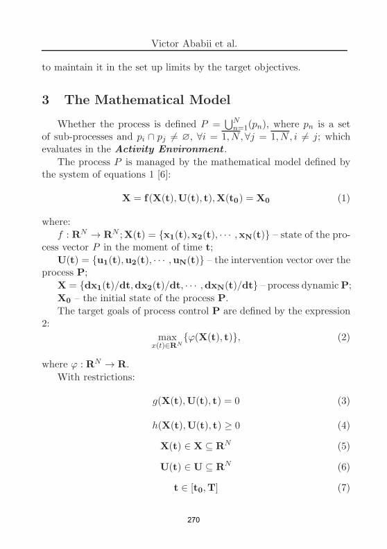
Victor Ababii et al.
to maintain it in the set up limits by the target objectives.
3 The Mathematical Model
Whether the process is defined P =⋃
N
n=1(pn), where pn is a set
of sub-processes and pi ∩ pj 6= ∅, ∀i = 1, N,∀j = 1, N, i 6= j; whichevaluates in the Activity Environment .
The process P is managed by the mathematical model defined bythe system of equations 1 [6]:
X = f(X(t),U(t), t),X(t0) = X0 (1)
where:
f : RN → RN ;X(t) = x1(t),x2(t), · · · ,xN(t) – state of the pro-
cess vector P in the moment of time t;
U(t) = u1(t),u2(t), · · · ,uN(t) – the intervention vector over theprocess P;
X = dx1(t)/dt,dx2(t)/dt, · · · ,dxN(t)/dt – process dynamicP;
X0 – the initial state of the process P.
The target goals of process control P are defined by the expression2:
maxx(t)∈RN
ϕ(X(t), t), (2)
where ϕ : RN → R.
With restrictions:
g(X(t),U(t), t) = 0 (3)
h(X(t),U(t), t) ≥ 0 (4)
X(t) ∈ X ⊆ RN (5)
U(t) ∈ U ⊆ RN (6)
t ∈ [t0,T] (7)
270

Distributed System for Real-Time Collective Computing
To achieve the goals provided in 2 it is necessary to find the vectorU(t) respecting the conditions 3-7, which has to ensure the condition8, it means the solving strategy of the collective calculation problem:
∇ϕ(x(t))i =∂ϕ
∂x(t)i(X(t)) > 0,∀i = 1, N. (8)
4 The Topology of Multi-Agent Network
The collective calculation specific consists in taking decisions basedon the particular decisions of the agents. In this context, three typesof decisions can be classified:
- Absolute decisions – when all the particular decisions of the agentsare taken into consideration;
- Majority decisions – when the particular decisions of most agentsare taken into consideration;
- Minority decisions – when the personal decisions of the agents thatcorrespond to the personal agents’ interests are taken into account.
The topology of the multi-agent collective computing network isshown in 4
Figure 2. Multi-Agent network for Collective Computing.
In 4 there is presented the set of Agents A1, ..., AN that forms anetwork Mesh. Each Agent acquires the status xi of the process P,processing the data according to the algorithm defined by mathematicalmodels 1-8 and influences the process with the command value ui.
271

Victor Ababii et al.
5 The distribution of collective computing
tasks
In order to optimize the process of calculating and uniform dis-tributing of computational power, the following solution is proposed,where each Agent will perform the set of instructions defined by themathematical model 9:
Ai :
gi(X(t),ui(t), t) = 0,
hi(X(t),ui(t), t) ≥ 0,
fi(X(t),ui(t), t) = dxi(t)/dt,maxx
i(t)∈RN ϕi(X(t), t),
QoSi = qi(ui(t)),Tk−1 < t ≤ Tk,
∀i = 1, N,
(9)
where: QoSi – quality criterion of the command service; qi – function toevaluate the quality criterion; Tk−1 – the beginning of the time intervaland Tk – the end of the time interval for the evaluation quality criterion.
The quality criterion QoS is evaluated in the graph shown in 5,where: QoSmax – the maximum quality criterion; QoSopt – the optimalquality criterion; QoS(t) – the evolution of the quality criterion in time;C(t) – the convergence of the command value solution in time; Tk−1 –the beginning of the evaluation of the quality criterion QoS; Tk – theend of the time interval of quality criteria evaluation QoS ; U(Tk) –the values of the command vector obtained at the moment of time Tk.
At the beginning of each data processing cycle Tk−1 there is ac-quired the state vector X(t), performed by all Agents connected to thenetwork, and the communication between them with this data. At theend of the data processing cycle Tk the action on the process P withvector values U(Tk) takes place.
6 Conclusion
The results of this research are dedicated to solve some specificproblems of real-time collective calculation. The collective computa-
272

Distributed System for Real-Time Collective Computing
Figure 3. The graph of the quality criterion evolution QoS.
tion is presented as a Multi-Agent system which solves a complex prob-lem defined in time (a process). In this paperwork there are presented:the hierarchical structure of the collective calculation system that de-termines the interaction between different abstract levels of the system;the mathematical model that describes the evolution of the process intime with the definition of the target goals, and the strategic meth-ods applied in solving of the problem; the topology of the Multi-Agentnetwork that presents a Mesh network; and the mathematical modelfor the distribution of computational tasks among the set of Agents.In order to synchronize the collective calculation process performed bythe set of Agents, the quality criterion evaluated in time is defined. Forthe future, a Multi-Agent system based on the NodeMCU V3 ESP8266and ESP32 devices development is planned. As a complex problem, theorder of a production process is selected, which includes the stages of:logistics, production, marketing and delivery.
Acknowledgments. The results presented in this paperwork wereobtained in the Laboratory of ”Artificial Intelligence” of the Depart-ment of Computer Science and Systems Engineering and are a partof the theme of institutional research, Project 15.817.02.28A ”Mod-els, methods and interfaces for the management and optimization ofintelligent manufacturing systems”.
273

Victor Ababii et al.
References
[1] G. Coulouris, J. Dollimore, T. Kindberg, G. Blair. Distributed Sys-
tems: Concepts and Design. & Fifth Edition, Pearson Education,
publishing as Addison-Wesley, 2012,1067p. ISBN:978-013-214301-1.
[2] M. Dragoicea. Sisteme ın timp real. Dezvoltare pe baza de model.
& Editura Universitara, Bucuresti, Romania, 2010, 370p. ISBN:978-973-749-924-0.
[3] A. Fischer, S. Greiff, J. Funke. The Process of Solving Complex
Problems. & Journal of Problem Solving, 4(1), pp. 19–42, February2012. DOI: 10.7771/1932-6246.1118.
[4] T. Malica. Collective Intelligence vs. Artificial Intelligence – Review
& International Journal of Emerging Technology and Advanced En-
gineering, Vol. 2, no. 7, July 2012, pp. 198–199. ISSN: 2250-2459.
[5] A. Dorri, S. Kanhere, R. Jurdak. Multi-Agent Systems: A survey &IEEE Access, April 2018. DOI: 10.1109/ACCESS.2018.2831228.
[6] I. Necoara. Metode de Optimizare Numerica. & Universitatea Po-
litehnica din Bucuresti, Ed. Politehnica Press, 2013, 278p.
Victor Ababii1, Viorica Sudacevschi1, Mariana Osovschi1, Ana Turcan1, AnaNistiriuc1, Dimitrie Bordian1, Silvia Munteanu1
1 Department of Computer Science and Systems Engineering,Technical University of MoldovaE–mail: [email protected]
274

Proceedings of the Fifth Conference of Mathematical Society of Moldova
IMCS-55, September 28 - October 1, 2019, Chisinau, Republic of Moldova
Encapsulating the Concept of Information in
Scientific Paradigm of Reality: A Possible
Scenario of a Theory of Everything
Veaceslav Albu
Information is information, not matter or energy.
No materialism, which does not admit this, can
survive at the present day.
Norbert Wiener
Abstract
The paper represents an attempt of formulating a theory ofeverything as a coherent theoretical account how nature workswhere information gets its fundamental role with same impor-tance that the energy and the matter have in main theories ofmodern physics. The presented approach, based on central con-cepts of N. Wiener and B. Mandelbrot is able to solve many ex-isting paradoxes yielded by contemporaneous scientific paradigm.
Keywords: potential information, embedded information,emergent information, universal gravity, observer, homeostasis,Unified Field Theory.
1 Introduction. What is going on here?
To propose a theory of everything today presupposes that one should beprominently skilled in theoretical or quantum physics. Otherwise, thisperson has maximum probability to fail in his goal to challenge the stateof the art theories of modern cosmology. The above-mentioned twofields of physics harmonized together by Einstein’s theory of relativity,
c©2019 by Veaceslav Albu
275

Veaceslav Albu
play the same role as a central black hole does in its own galaxy. Everysingle object within this galaxy has to obey the power of gravity ofthis central black hole and surround it within the given paradigm ofseemingly free flight. Unfortunately, the time of building up a theory ofeverything just by power of reason during the romantic contemplationof reality, as Plato and Aristotle did, is gone. Nevertheless, this paperpresents such an endeavor.
The aim of the proposed approach is to enrich the existing scien-tific paradigm with a central concept fromWiener’s cybernetics [1] – theconcept of information, and with the concept of fractals, Mandelbrot’s[2] view on how the nature topologically behaves. From this point, someminor complications begin. Although, the proposed paradigm remainsacting in four-dimensional reality, there is one exception: the concept
of relative change of information in a given fractal of observed real-ity relocates the concept of time. Another minor novelty required byour reasoning and aimed to reach the harmony of the proposed theory,is that the force of gravity transforms into four-dimensional universalforce, where the other free known forces, unified as electromagneticforces remain three-dimensional. Moreover, the known force of gravityremains in 3D space as the 3D projection of the four-dimensional uni-versal gravity. That novelty does not contradict with their definitionsas forces acting within three-dimensional matter. Consequently, thethree-dimensional potential energy resulting from Newtonian gravity,in the proposed theory becomes four-dimensional as well.
The very new concepts in this theory are the concept of potential
information, the concept of embedded in 3D matter information andthe concept of emergent information in given volume of 3D space thatwe will explain later in this paper.
2 Why information?
We believe there are two reasons why the information concept is funda-mental in nature but is missing in contemporaneous scientific paradigmof reality. The first reason suggests that we are living in informational
276

Encapsulating the Concept of Information in Scientific Paradigm . . .
age due to the courage of Norbert Winner to put scientists from non–linked sciences as engineers, biologists, chemists, and psychologists tobrainstorm together. He did that with one purpose – to find a newperspective how to build an informational hammer for humans withthe same revolutionary results, as the stone hammer had for our an-cestors. Wiener’s citation from the top of this paper represents thefinal two sentences that coronate the “Computing Machines and theNervous System” chapter in his “Cybernetics”. Unfortunately, sincethen no one of the modern cosmology theorists did pay attention tothe highest intuition of this idea. By that, they gave a chance to thepresent attempt to be produced as a remembrance of Wiener’s warn-ings – that there is no way to build a scientific paradigm without useof information as a fundamental block of reality. The second reason,which makes us believe that the concept of information follows fromthe natural laws of the Universe, represents the fact of absolute simi-larity of mathematical description of dependence at opposite scales ofreality – Newton’s formula for the force of gravity and for Coulomb’sformula for the force between two charges.
3 The Theory’s Road Map. The information
The main concept observed in nature that inspired N. Wiener to cre-ate the science of cybernetics was the concept of homeostasis in livingorganisms as a necessary element for sustaining the evolution of life.He proposed the seminal idea of embedding the same principles intoautomatic machines and computers as fundamental for cybernetics. Hegot this insight from his attempt to find an efficient solution for guidedmissile technology during WWII by implementing the feedback princi-ple. Its automatic missiles system uses the received information abouta targeted airplane’s current position to a simultaneous change of pa-rameters of the missile’s flight towards the target. It is easy to followthe analogy between guided hunting on airplanes and the Schrodinger’scat paradox. Indeed, the one hunting on airplane during the nighttimewithout feedback of its actions does not know if airplane is still flying
277

Veaceslav Albu
or it is dead, by analogy with a cat from the box. The first importantconclusion follows from above reasoning. The feedback information innature and in cybernetic systems’ processors plays a role of an ob-
server, one of very fundamental concept of quantum mechanics. So,if information is so important, then why it is missing as a fundamentalconcept in modern scientific paradigm?
The second important conclusion follows from the ability of hu-mans’ and contemporaneous Artificial Intelligence (AI) ”beings” forplanning its future strategies and actions. Any plan of the future, inone’s mind or in computer’s processor, represents a pure informationalpicture of future imagined state of affairs. A good example can bea plan of launching a space ship. The proper start of a space ship,in the first day when a person becomes in charge of that space ship’slaunching, represents just a collection of thoughts and imaginations inthe person’s mind as pure non-material information. Nevertheless, apush on the START button on the day of launch makes this pure imag-inary and informational event real and it really pushes the spacecraftinto outer space. On the first day, that person’s mind entangles withthe future pure informational event and, by controlling his real actionswith feedback information of the current state of affairs on the projectwith the information from the imagined start moment, the launch ofthe space ship becomes real. One can count terabytes of feedback infor-mation about state of affairs during the implementation of the project,but only at the launching moment we will open the ”Schrodinger cat’sbox cover”, and we will see if all feedback information was correctly ob-served and processed. The second conclusion has a twofold structure:First, human mind possesses properties of a quantum device, which canentangle itself with an imagined informational object from future real-ity. Second, the quantum state of observer can be applied by humanor AI ”beings” minds to any logically possible imagined targeted eventfrom the future reality, by using feedback information for adjusting itsreal actions with future’s target event to make it become real.
The following question then arises. If we admit that living organ-isms, non–living structures in nature and robotic systems possess the
278

Encapsulating the Concept of Information in Scientific Paradigm . . .
self–organizing property, what impedes us to admit that the abilityof self–planning is also necessary for nature, as a necessary a prioripart of self–organization? If we acknowledge all the above said, weshould confess that N.Wiener was right and wise, when he spelled outfor us his famous idea. If so, one should recognize that informationis information, not matter and not energy and it is fundamental fornature, as matter and energy does. For the purpose of present theory,information persists in three well–determined states — potential in-
formation, emergent information and information embedded
in matter. The latter one, which is most widely known by humanity,reveals itself in all material objects or phenomena. Digging embeddedinformation from matter by any specific science generates knowledge ofthat science. Humans perceive the embedded information as a physicalobject with the same degree of illusion, as they perceive a movie as awhole by looking at a CD with this movie. The emergent informationreveals itself on the cloud of processes emerging on the edge of thefractal dimension for each recurrent internal fractal of the Universe’sfractal. As an example, one can take emergent information about out-puts of different quantum effects occurring in cells of living organismson atomic and molecular level, as well as in all Universe’s stars evo-lution processes. The emergent information ontologically precedes theembedded information. Finally, the potential information is a stateof information that persists as embedded in four–dimensional universalgravity of a ”genuine immaterial form” of energy–information singular-ity of matter by analogy with singularity state of matter in Universe’sblack holes. The potential information represents all logically possibleform of emergent or embedded information. As an example of genuinepotential information, one can take the thoughts generated by theirmind. The Universe’s fractal can be seen as an homeostasis in actionin 4D space, where Big-Bang can be taken as burst of correspondingpotential information into 3D space as primary emergent informationvia quantum realm, that formed the all atoms in Universe and pro-ceed to step of creating of embedded information in 3D space, knownas matter and energy. All the above conclusions roots in N. Wiener’s
279

Veaceslav Albu
legacy.
4 The force
A hard problem of the proposed theory is to find the carrier of allinformational events described above. As a universal force, whichgenerates all energy appearance in 3D space, we propose the four–dimensional gravity that represents state of energy–informational sin-gularity, bounded by some laws of 4D energy–information conservationby analogy with its 3D analog. Moreover, the proposed four dimen-sionality of force of gravity do represent also an attempt to presenta possible solution for unsolved yet Unified Field Theory, as for 3Dspace all four forces are governed by the proposed four dimensionalityof universal gravity, as fourth dimension of our reality. Saying that,we have no logical impediment for claiming existence of phenomenonof homeostasis within such singularity that can locally activate respec-tive amount of potential energy from where the fractal of our Universeroots. Following, from the definition of homeostasis we can logicallydeduct the existence of a feedback organized as cause-and-effect chainof generating emergent and embedded in 3D space information, un-der the conditions controlled by given set of our Universe’s constants.Such feedback forms a circuit or a loop, with Bing Bang singularityas an output and routed back through black holes’ singularities as aninput, or vice versa. Important is that such system feeds back intoitself developing as our Universe’s fractal. In addition, we shall ad-mit logically possible existence by that of many others feedback loopsas other universe’s fractals possibly governed by the same or anotherset of universal constants. For that reason, we shall admit the exis-tence of four-dimensional force carrier, which reveals itself in 3D dueto Heisenberg uncertainty principle, depending on released emergentinformation in the given point of space. As in the proposed paradigmthe reality is four-dimensional, the commonsensical reasoning in mod-ern physics of the dimensionless point in 3D space should be relocatedto +1 dimension of information point, or four-dimensional point, in 4D
280

Encapsulating the Concept of Information in Scientific Paradigm . . .
space.
5 The fractals
Finally, to complete the performance of the great spectacle of our Uni-verse’s evolution conducted by the proposed theory, we need a ”stage”,materiality of which will be easy to defend from any attempts to claimthe idealistic nature of the proposed theory, as N. Wiener suggested.Legacy of another modern great thinker, B. Mandelbrot [2] claims thatfractals are the ideal carriers of all infinitely complicated objects inthe nature. They have some specific properties that are very appro-priate for fulfilling the needs of our ”stage”. Indeed, fractals possessan emergent hierarchical self–similar structure. Internal fractals repeatthe structure of external ones and vice versa. We will take density ofemergent information in matter directed by laws of quantum physics ingiven volume of 3D space as fractal dimension. That fractal dimensionis the same for entire hierarchical structure of our Universe’s fractal.As fractal in Universe acts for 3D matter, together with fractal dimen-sion, mentioned above the dimension of any 3D fractal has to have afractional fractal dimension between 3 and 4 integer. As B. Mandelbrotdid not describe such entity as the Universal fractal, for the sake of pre-sented theory we will take the following fractal’s definition: ”Fractalsare the emergent properties of iterative feedback systems that exhibitboth unpredictable and deterministic behaviors, forming patterns thatmanifest as complex coherent structures, with the property of scaleinvariance and self-similarity, displaying very specific boundary condi-tions, with complex morphologies that have a fractal dimension thatuniquely quantifies the level of complexity of the emergent patternswithin the system” [3]. Important are the specific particularities ofUniverse’s fractal, see [4]. Each fractal manifests itself between its ownpair of singularities and only both emergent and embedded informationtranscend such singularities. The homeostasis and feedback loop, inclu-sively between level of emergent information and embedded informationlevel, remains the main principle under what the self–organization of
281

Veaceslav Albu
matter occurs in given fractal. As an example of such fractals, we canmention from the single living cell up to a living body, any plant orcoral, any star system, etc.
6 Conclusion
The paper presents the possible scenario for theory of everything, whichencapsulates the concept of information in modern scientific paradigmof reality with a clear aim, to prove the N. Wiener’s wise vision ofspecific and fundamental role of information for performance of reality.The presented approach keeps the existing four dimensions of reality,but as the fourth dimension, the theory regards the four-dimensionalgravity, as universal carrier of all changes of real world.
References
[1] N. Wiener. Cybernetics: Or Control and Communication in the
Animal and the Machine, MIT Press, 1961.
[2] B. Mandelbrot. The fractal Geometry of Nature, Times Books,1982.
[3] L. Gardi. The Mandelbrot set and the fractal na-
ture of light, the Universe, and everything, 2013.http://proceedings.spiedigitallibrary.org/. Terms of Use.http://spiedl.org/terms
[4] V. Albu. An Inquiry into Indispensability of Information in Hylo-
morphic Unity of the Universe and the Phenomenon of Life, MAthesis submitted to the University of Wales Trinity Saint David,Lampeter, UK, 2018.
Veaceslav Albu
Vladimir Andrunachievici Institute of Mathematics and Computer Science, MoldovaE–mail: [email protected]
282

Proceedings of the Fifth Conference of Mathematical Society of Moldova
IMCS-55, September 28 - October 1, 2019, Chisinau, Republic of Moldova
Rule Forms in Rewriting Systems
Artiom Alhazov, Rudolf Freund, Sergiu Ivanov
Abstract
We discuss which sets of patterns for rules are sufficient forreaching computational completeness in various rewriting sys-tems, for example, sequential generating grammars and acceptingmachines as Turing machines and circular Post machines; specialattention is paid to the parallel model of membrane systems.
Keywords: theoretical computer science, rewriting systems,membrane computing, normal form.
1 Introduction
Following various normal forms for type-0 grammars and register ma-chines, we aim at a systematic investigation of the forms of rules suf-ficient to reach computational completeness, besides sequential mod-els also focusing on the parallel model of membrane systems. In thiscontext we see computational completeness as the capability of a for-mal computing model to generate or accept all recursively enumerablesets of strings (in the case of string rewriting systems) and all recur-sively enumerable sets of vectors of non-negative integers (in the caseof multiset rewriting systems). In this context we allow for ignoring abounded amount of superfluous symbols (for example, the state sym-bol or catalysts) and/or a bounded amount of strings (e.g., the emptystring/multiset).
The formal computing models of our interest are limited to string ormultiset rewriting systems, working in the sequential or parallel deriva-tion mode. Questions about descriptional complexity parameters, such
c©2019 by Artiom Alhazov, Rudolf Freund, Sergiu Ivanov
283

Artiom Alhazov, Rudolf Freund, Sergiu Ivanov
as the size of the alphabet or sub-alphabets or the number of mem-brane labels, catalysts etc., are out of the scope of this paper, yet wemainly focus on the maximal number of rule forms and the maximallength of the strings describing these rule forms.
2 Definitions
For the standard definitions and the main results in formal languagetheory we refer the reader to handbooks as, for example, [10].
The simplest variant of a rewriting system can be defined as a tuple(V,R), where V is a finite alphabet and R ⊂ V
∗ × V∗ is a finite set
of string or multiset rewriting rules; (u, v) ∈ R is typically written asu → v. Of course, this basic variant does not yet specify
1. the initial string or multiset w,
2. sub-alphabets, for example the terminal alphabet for extendedgrammars or the states for machines,
3. special sub-alphabets (for additional restrictions/normal forms,e.g., catalysts),
4. the derivation relation ⇒, for example, xuy → xvy | x, y ∈
V∗, (u, v) ∈ R for sequential grammars,
5. the halting condition, for example, the absence of non-terminalsymbols for grammars, the appearance of the final state for ma-chines, or the inapplicability of any further rule in the case of Psystems.
We should also mention that rules may be more complicated thanu → v in case of certain control mechanisms or distributed systems, andthe notation sometimes needs to include special symbols to representadditional ingredients (e.g., permitting/forbidden context, membranelabels/polarizations), yet in principal we shall restrict ourselves to thebasic rule forms in this paper:
284

Rule Forms in Rewriting Systems
A rule form is a pattern of the form u → v, where u, v are strings ofvariables (and, possibly, special symbols). For some formal computingmodelM , we say that a system G of typeM is constructed according toa finite set F of rule forms if each rule of G is obtained from some ruleform in F by replacing each variable by an element from an alphabetspecified for this variable. In the most common case, we distinguishbetween the total alphabet V , the set of terminal symbols T (⊆ V )and the set of non-terminal symbols N := V \ T .
For example, A → BC (A,B,C ∈ V ) is a rule form, but A → u
(A ∈ V , u ∈ V∗) is not a rule form, as it can only be written as an
infinite set of rule forms, one for each value of |u| ∈ N.
We say that a set F of rule forms is sufficient for obtaining computa-tional completeness for some formal computing modelM if the family ofsets of strings or vectors of non-negative integers generated or acceptedby systems of M using only rules constructed according to F equals RE
(the family of recursively enumerable string languages) or PsRE (thefamily of recursively enumerable sets of vectors of non-negative inte-gers), thereby possibly ignoring specific symbols or a bounded numberof strings or multisets.
3 Sequential rewriting systems
We proceed with presenting rule forms for computationally completesequential string rewriting models. This is certainly not a completelist, but we cover some known interesting cases.
3.1 String grammars
In case of sequential string grammars, two rule forms are sufficient:A → BC and AB → C. Indeed, all that is needed for computationalcompleteness is cooperation and the ability to lengthen and shortenthe sentential form. As a technical detail, we mention that we neglectthe empty string to be generated, which would require additional rulesof the form A → λ. We will omit such a comment throughout the rest
285

Artiom Alhazov, Rudolf Freund, Sergiu Ivanov
of the paper as long it is obvious from the context.
If we consider accepting, no matter by halting or by final state, thena single rule form AB → CDE is enough, because we can use copies ofan additional symbol E for lengthening especially the right-hand sideof rules, i.e., we take AB → CEE instead of AB → C. Informationcan propagate over these “garbage” symbols E and these symbols donot influence accepting.
These results are classic and straightforward, so the proofs can beleft to the reader.
Other remarkable examples of rule forms for the type-0 grammarscan easily be derived from some well-known normal forms:
3.1.1 Penttonen normal form
In [7] it is shown that every recursively enumerable language can begenerated by a type-0 grammar with rules of the forms A → BC,AB → AD, A → a, and E → λ, where A,B,C,D,E are non-terminalsymbols in N and a is a terminal symbol in T .
Based on these rule forms, we immediately infer that we only needrule forms A → BC, AB → AD, and E → λ, where A,C,D,E arenon-terminal symbols in N and B ∈ N ∪ T , as every rule A → a canbe replaced by the rules A → aE and E → λ. In fact, only one suchrule E → λ is needed.
3.1.2 Geffert normal form
Among other variants, in [4] it is shown that every recursively enumer-able language can be generated by a type-0 grammar with rules of theforms S → uSv and S → u, where S is a special non-terminal sym-bol and u, v ∈ (A,B,C,D ∪ T )∗, where A,B,C,D are non-terminalsymbols and T is the set of terminal symbols, as well as the two non-context-free λ-rules AB → λ and CD → λ, which constitute the ruleform XY → λ. Introducing intermediate non-terminal symbols, therules of the forms S → uSv and S → u can be replaced by rules only
286

Rule Forms in Rewriting Systems
using the single rule form X → Y Z. In total, only the two rule formsX → Y Z and XY → λ are needed for obtaining computational com-pleteness, which strengthens the result given at the beginning of thissection.
3.2 Insertion-deletion systems
Insertion-deletion systems are another grammar-like computing model,with rules of the form λ → v and u → λ, u, v ∈ V
∗.
Two rule forms are already sufficient (for example see [5] and [6]),e.g., we only need λ → AB and ABC → λ; alternatively, one can useλ → ABC and AB → λ.
3.3 Multiset grammars
If the underlying data structure is a multiset instead of a string, thenwithout additional control the power of sequential systems is equivalentto the power of partially blind register machines, i.e., they are notcomputationally complete.
Of course, using additional mechanisms, computational complete-ness can be reached again. For example, we can use inhibitors, thus ob-taining rule forms AB → C and A → BC|¬F , where |¬F in A → BC|¬Findicates that the rule A → BC can only be applied if no F appearsin the underlying sentential form. Not surprisingly, a single rule formAB → CDE|¬F is enough in the accepting mode. In Section 5 weavoid inhibitors by switching from the sequential derivation mode tothe maximally parallel derivation mode.
4 Turing machines and circular Post machines
For Turing machines, in general the transition rules are of the form(p,A) → (q,B, d), where p, q ∈ Q are states, A,B ∈ V are tape sym-bols, and d ∈ L,R is the direction of the head move. As rewritingrules, these transition rules can be written/simulated as follows:
287

Artiom Alhazov, Rudolf Freund, Sergiu Ivanov
• (p,A) → (q,B,R) is simulated by pA → Bq, and
• (p,A) → (q,B,L) is simulated by CpA → qCB, for any C ∈ V .
However, at the expense of intermediate states, it is possible to splitrules into two categories: rules with rewriting, but without moving andrules without writing but moving, which, in Turing machine notation,yields transition rules of the form (p,A) → (r,B, S), where S indicatesthat the tape head stays on its position, as well as (r,B) → (q,B,R)and (r,B) → (q,B,L), respectively. These transition rules correspondwith rewriting rules in the following way:
• the rules (p,A) → (r,B, S) and (r,B) → (q,B,R) are simulatedby pA → rB and rB → Bq, and
• the rules (p,A) → (r,B, S) and (r,B) → (q,B,L) are simulatedby pA → rB and Cr → rC, for any C ∈ V .
The relevant rule forms then are PA → RB, RB → BR, andBR → RB, with P,R ∈ Q and A,B ∈ V .
An interesting variant of Turing machines is called circular Postmachines: the tape is circular, moving is always to the right, but it ispossible to delete and insert tape cells. Circular Post machines can beinterpreted as string rewriting systems (Post systems of a very specifictype) where the symbols are consumed on the left and written on theright.
We now present rule forms derived from the normal form calledCPM5 (for example, see [2]):
pA → q and p → Aq, with p, q ∈ Q and A ∈ V .These rules are to be interpreted as working on circular strings, chang-ing the state from p to q, together with deleting symbol A on the leftor inserting it on the right, respectively.
5 P systems
We now turn our attention from sequential to parallel rewriting sys-tems. As a special model of that kind, we consider membrane systems,
288

Rule Forms in Rewriting Systems
i.e., P systems, with non-extendable multisets of rules acting on multi-sets in parallel, and the computation halts if no rule can be applied anymore. Whereas the general model of P systems allows for the evolutionof objects in different membrane regions as well as the passing of theobjects through the membranes to inner membrane regions or to theouter membrane region, we here restrict ourselves to the trivial case ofone-membrane systems. We refer to [8] and [9] for the main definitionsand results in the area of membrane systems as well as to the P systemswebsite [11] for actual news in this area.
Even in one-region P systems, the rule forms A → BC and AB → C
are sufficient for obtaining computational completeness in the gener-ating case, and the single rule form AB → CDE is enough for theaccepting case. These rule forms are similar to the ones being suffi-cient in the case of sequential string grammars, whereas we remind thereader that in the multiset case the sequential application of multisetrules of these forms is not enough.
Co-operativity can be restricted in various ways. For example, usinganti-matter objects and anti-matter rules, we get a Geffert-like set ofrule forms A → BC and AB → λ (e.g., see [1]).
5.1 Purely catalytic P systems
Using catalytic rules only, we get rule forms cA → cB1 · · ·Bk | k ∈ F,where c ∈ C stands for one of the symbols in the set of catalysts C, i.e.,symbols which are never changed, and the Bi represent other symbols/∈ C. For a given finite set F the lengths of the right sides are bounded,therefore this is a finite set of rule forms. As already shown in [3],F = 0, 1, 2, 3 is sufficient in the generating case. Using an additionaldummy symbol e, we immediately get that F = 0, 3 is sufficient,too. As F = 0, 1 would not allow the underlying multiset to grow,the challenging question for future research is whether F = 0, 2 isalready sufficient, too.
289

Artiom Alhazov, Rudolf Freund, Sergiu Ivanov
6 Further variants
In the case of sequential string grammars, further variants of rule formsnecessary and sufficient for obtaining computational completeness maybe investigated, especially based on different variants of the Geffertnormal form.
In the case of parallel rewriting systems, especially many furthervariants of P systems remain to be investigated carefully, for example,P systems with membrane generation and membrane dissolution as wellas P systems with active membranes.
7 Conclusions
We have presented a number of generating and accepting devices andcorresponding sets of rule forms sufficient for obtaining computationalcompleteness. We first discussed sequential grammars as well as Tur-ing machines and circular Post machines as specific models for com-putations on strings. For sequential string grammars, several sets ofrule forms sufficient for obtaining computational completeness were de-scribed, especially using specific well-known normal forms as the Pent-tonen normal form and the Geffert normal form.
Moreover, we then considered the model of membrane system (Psystems), where multisets are evolving by applying non-extendablemultisets of rules in parallel. We have especially focused on one-membrane P systems and investigated rule forms necessary for severalvariants of P systems. For purely catalytic P systems we have raisedthe challenging open question if the number of non-catalysts on theright-hand side of the catalytic rules can be restricted to two, whereaswe know that three of them are sufficient in the generating case.
Finally, we shortly discussed further variants to be investigated inthe future.
290

Rule Forms in Rewriting Systems
References
[1] A. Alhazov, B. Aman, and R. Freund. P systems with anti-matter.In M. Gheorghe, G. Rozenberg, A. Salomaa, P. Sosık, and C. Zan-dron, editors, Membrane Computing - 15th International Confer-
ence, CMC 2014, Prague, Czech Republic, August 20-22, 2014,
Revised Selected Papers, volume 8961 of Lecture Notes in Com-
puter Science, pages 66–85. Springer, 2014.
[2] A. Alhazov, A. Krassovitskiy, and Yu. Rogozhin. Circular Postmachines and P systems with exo-insertion and deletion. InM. Gheorghe, Gh. Paun, G. Rozenberg, A. Salomaa, and S. Verlan,editors, Membrane Computing – 12th Int. Conference, CMC12,
Fontainebleau, volume 7184 of Lecture Notes in Computer Science,pages 73–86. Springer, 2012.
[3] R. Freund, L. Kari, M. Oswald, and P. Sosık. Computationallyuniversal P systems without priorities: two catalysts are sufficient.Theoretical Computer Science, 330(2):251–266, 2005.
[4] V. Geffert. Context-free-like forms for the phrase-structure gram-mars. In M. Chytil, L. Janiga, and V. Koubek, editors, Mathemat-
ical Foundations of Computer Science 1988, MFCS’88, Carlsbad,
Czechoslovakia, August 29 - September 2, 1988, volume 324 of Lec-ture Notes in Computer Science, pages 309–317. Springer, 1988.
[5] M. Margenstern, Gh. Paun, Yu. Rogozhin, and S. Verlan. Context-free insertion-deletion systems. In E. Csuhaj-Varju, C. M. R.Kintala, D. Wotschke, and Gy. Vaszil, editors, 5th Interna-
tional Workshop on Descriptional Complexity of Formal Systems –
DCFS 2003, Budapest, Hungary, July 12 - 14, 2003. Proceedings,pages 265–273. MTA SZTAKI, Hungarian Academy of Sciences,Budapest, Hungary, 2003.
[6] M. Margenstern, Gh. Paun, Yu. Rogozhin, and S. Verlan. Context-free insertion-deletion systems. Theoretical Computer Science,330(2):339–348, 2005.
291

Artiom Alhazov, Rudolf Freund, Sergiu Ivanov
[7] M. Penttonen. One-sided and two-sided context in formal gram-mars. Information and Control, 25(4):371–392, 1974.
[8] Gh. Paun. Membrane Computing: An Introduction. Springer,2002.
[9] Gh. Paun, G. Rozenberg, and A. Salomaa, editors. The Ox-
ford Handbook of Membrane Computing. Oxford University Press,2010.
[10] G. Rozenberg and A. Salomaa, editors. Handbook of Formal Lan-
guages. Springer, 1997.
[11] The P Systems Website. http://ppage.psystems.eu/.
Artiom Alhazov1, Rudolf Freund2, Sergiu Ivanov3
1Vladimir Andrunachievici Institute of Mathematics and Computer Science.Academiei 5, 2028 Chisinau, MoldovaE–mail: [email protected]
2Faculty of Informatics, TU Wien.Favoritenstraße 9-11, 1040 Wien, AustriaE–mail: [email protected]
3IBISC, Universite Evry, Universite Paris-Saclay23, boulevard de France, 91034 Evry, FranceE–mail: [email protected]
292

Proceedings of the Fifth Conference of Mathematical Society of Moldova
IMCS-55, September 28 - October 1, 2019, Chisinau, Republic of Moldova
Can Computers Catch the Authors Style?
Victoria Bobicev, Yulia Hlavcheva, Olga Kanishcheva
Abstract
The paper presents the experiments on authorship attributionfor scientific articles written in Russian and Ukrainian. The mainaim of this research is to explore the topic influence on authorclassification.
Keywords: Text classification, authorship attribution, topicclassification, machine learning methods, character based learn-ing.
1 Introduction
Authorship Identification is a hot topic in many areas and especiallyin science and education as a part of plagiarism detection effort. Thegoal of this study is to verify how strong the topic of the text influ-ences its authorship attribution. We used machine learning methods toclassify the scientific articles from different domains by their authors.While the domain specific words could affect the classification, we se-lected sets of texts from the same domain and performed authorshipattribution within the domain. However, even within one domain thepapers describe different topics that still affect the classification. Weare organizing the experiments in such a way that training and testsets contain different papers of the same author in order to avoid topicinfluence.
c©2019 by Victoria Bobicev, Yulia Hlavcheva, Olga Kanishcheva
293

Victoria Bobicev, et al.
2 Related work
The methods used in the domain of authorship attribution vary frompurely manual meticulous analysis of the different text elements tothe absolutely automate statistical methods such as machine learning.While machine learning is mostly a classification task, classification bythe text author is always influenced by the text topic. This phenomenawas explored in [1] and the results showed that most of the stylometricvariables are actually discriminating topics rather than authors.
Our work is the continuation of the author classification experi-ments presented in [2] on the scientific papers written in Russian andUkrainian language. Although there has been made an attempt toavoid the topic influence by experimenting with the papers form onedomain (Economics), there was still a significant probability that top-ics of the papers influenced the classification and helped to obtain suchhigh results (f-measure from 0.85 to 0.95 on different datasets). In thispaper we reorganize the experiments in order to avoid topic classifica-tion as much as possible.
3 Experiments Description
The Dataset. We used the same dataset described in [2]. There weretwo data sets: (1) the whole one that included 271 Ukrainian and 77Russian articles written by 32 and 8 authors respectively (we experi-mented with them apart) and (2) the part consisting of 175 Economicsand 65 IT articles written by 18 and 10 authors respectively (experi-mented apart as before).
The Method. We worked with classification method on the baseof PPM compression algorithm. It demonstrated its ability to classifythe short forum posts by the author with impressive accuracy of almost90% [3]. The method uses as the features all sequences of characters oflength 5, 4, 3, 2 and 1 character from texts. We tested two variations ofthis method: (1) absolutely all characters from texts including upperand lower case letters, numbers, spaces, all kind of punctuation marks
294

Can Computers Catch Authors Style?
and other specific characters which appear in scientific publications;(2) only words composed of alphabet letters converted to lowercaseand spaces between them.
Text Organization. The main difference from the previous ex-periments consist in the text organisation. The main problem with thetext we worked with was the differences in their sizes: it differs from150 words to 50 pages and such differences may influence the classifi-cation results. This was the cause for the decision to split all texts infragments of approximately 150 words and classify these fragments byauthor. However, we suppose that the fragments of the same articlewere classified not by their author but by their common topic. Thus,in the current set of experiments we does not divide the texts in frag-ments and work with them as they are dividing them in training andtest sets in such way as every author is presented in both sets. We used5-fold cross-validation and there were around 2 texts from each authorin each test set.
Table 1. Results of the author classification experiments using PPMand two variations of the features: all characters (PPM char) and onlylowercase letters (PPM letters) on four sets of texts
Ukrainian Russian Economics IT
PPM(char) 0.601 0.950 0.604 0.800
PPM(letters) 0.585 0.913 0.580 0.782
Table 1 presents the results of the experiments. In comparisonwith the previous work we can say that high results remained only forRussian texts. The previous were 0.972 and 0.979; slightly higher. Forthe rest of the sets the results are much worse. For example, previousresults for Ukrainian were 0.854-0.865 and for IT 0.943-0.958. In caseof Russian texts, the high results are explained by the differences intopics the 8 authors in question wrote about.
295

Victoria Bobicev, et al.
4 Conclusion
In this paper we tested the hypothesis that author classification ishighly influenced by the text topics. The results of our experimentsconfirmed this. There is still possibility that the differences of textsizes influenced the results; we plan to explore the possibilities to evenout the text sizes. The other plan is to investigate the influence of thenumber of the authors on the classification accuracy.
References
[1] George K. Mikros and Eleni K. Argiri. Investigating Topic Influ-
ence in Authorship Attribution. In Benno Stein, Moshe Koppel,and Efstathios Stamatatos, editors, SIGIR 07 Workshop, PAN2007.
[2] V. Bobicev, Y. Hlavcheva, O. Kanishcheva, V. Lazu. Author-
ship Attribution in Scientific Publications, Corpora 2019, St-Petersburg, Russia.
[3] V. Bobicev, M. Sokolova, El Emam Khaled, Y. Jafer, B. Dewar, E.Jonker, S. Matwin. Can Anonymous Posters on Medical Forums
be Reidentified? Journal of Medical Internet Research, 2013, Oct03; 15(10):e215.
Bobicev Victoria1, Hlavcheva Yulia2, Kanishcheva Olga3
1Technical University of Moldova.E–mail: [email protected]
2National Technical University “Kharkiv Polytechnic Institute”E–mail: [email protected]
3National Technical University “Kharkiv Polytechnic Institute”E–mail: [email protected]
296

Proceedings of the Fifth Conference of Mathematical Society of Moldova
IMCS-55, September 28 - October 1, 2019, Chisinau, Republic of Moldova
Risk Detection Algorithm Design: Officer Fall
Case Study∗
Andrei Braicov, Ivan Budanaev and Mircea Petic
Abstract
This paper is an overview of the latest research resultsachieved within the ongoing NATO SPS program project – WIT-NESS. In particular, some details are presented regarding the al-gorithm for the state detection of a security officer deployed onthe ground. We will focus on the sudden fall or drop attack casestudies.
Keywords: surveillance, drone, sensor, data analysis, datafusion.
1 Introduction
The massive evolution of technologies has opened new ways to researchand solve problems from a wide range of fields: social-human; security;health; transport; monitoring etc. In the context of ensuring security,one of the problems is the detection of (crisis) risk situations for secu-rity agents. As an information provider in this case it can be a smalldigital device (not to burden the agent), with a sufficient operatingbattery life during a mission (up to 8-10 hours). Such a device can bethe agent’s mobile phone device. Modern smartphones are equippedwith a vast variety of sensors: gyroscope, accelerometer, magnetome-ter, Global Positioning System (GPS) proximity sensor, ambient lightsensor, microphone, fingerprint sensor, pedometer, barometer, heart
c©2019 by Andrei Braicov, Ivan Budanaev, Mircea Petic∗This research is sponsored by the NATO SPS Programme under the funding
NATO SPS G5437 - WITNESS - Wide InTegration of sensor Networks to EnableSmart Surveillance.
297

Andrei Braicov, Ivan Budanaev, Mircea Petic
rate sensor, thermometer, air humidity sensor, etc. The accelerometerdetects acceleration, vibration and tilt to determine the exact move-ment and orientation along the three axes: x, y and z. This sensorcan be used to determine the position of the phone (vertically or hori-zontally oriented), the position of the screen (facing up or down), thespeed of movement of the phone in any linear direction.
In the following section we will describe how we can use the ac-celerometer to detect the risk situation for the security agent – thefall.
2 Fall detection
The parameter provided by the fall analysis function (F ) is a very im-portant one, capable of improving the accuracy of detecting the criticalsituation. The fall of the police officer could signal a risk of attack onhim (injury, hit, etc.). The agent will carry the phone close to the waist(in a pocket, fastened by a belt clip, etc.).
Function F will have four modules:
1. the interoperability module will ensure the transition between thephone’s accelerometer and the system that will retrieve the data;
2. the motion data transformation module (acceleration values x, yand z ), provided by the accelerometer, will be passed through alow-order filter 1st order IIR (Infinite Impulse Response) [1] andwill be annotated and mapped into a comma-separated value fileformat (comma-separated value file format); each filtered accel-eration value will be stored locally for use in the next module(data analyzer);
3. the data analyzer will be responsible for processing and analyzingthe acceleration values (x, y and z ) to detect if these values repre-sent a drop. One can use a classification model based on decisiontrees from knowledge of past events [2]. This model is to be de-veloped a priori and will contain similar patterns of fall behavior.
298

Risk Detection Algorithm Design: Officer Fall Case Study
It will be kept in the cloud and will be filled with new patternsevery time the data analyzer finds a drop. Such a model, basedon decision trees, can be built from the SisFall dataset [3]. Thedecision tree is widely used for data classification and is one of thebest methods of classification and regression among many otherMachine Learning algorithms because it uses a non-parametricstructural design, which makes it efficient for managing data setswith large dimensions.
4. the alert manager will send notifications about the fall, includingto the cloud service (to update the mentioned model).
We mention that the methodology and the process of data collectionare of particular importance. This is why our decision was to collectdata collection in batches of different sizes (by default 10):
– vertical displacement of the phone, in particular if the phone falls25, 50 cm or more;
– horizontal displacement of the phone, the phone makes a suddenmove of 25, 50 cm or more on the x-axis;
– a derivative of previous observation – the agent falls (that is, itsuddenly reaches a horizontal position) with the phone in the pocketof the shirt;
– a derivative of previous observation – the agent falls (that is, itsuddenly reaches a horizontal position) with the phone near its belt.
Decisions on the first parameter regarding the risk situation can
be made based on the coefficient k =A
g, where A is the movement
acceleration of the phone, and g – the gravitational acceleration.
The acceleration A is given by the formula A =√
a2x + a2y + a2z,
with ax, ay, az being the accelerations of motion along the x, y andz-axes. The value of k will be close to 0 when the phone is idle (i.e.no sudden displacements). The value of k will exceed 1 as long as thephone is in motion. The value of k is close to 1 when the phone is infree fall, that is, when the phone falls, or when it has an equivalentto that displacement in other dimensions. Besides this approach, the
299

Andrei Braicov, Ivan Budanaev, Mircea Petic
model additionally relies on standard probabilistic methods to detectoutliers using z − score or standard deviation from the mean of thedata collected prior to model deployment.
3 Conclusion
The parameter provided by the fall analysis function is a very impor-tant one, capable of improving the accuracy of detecting the criticalsituation. The methodology and the process of data collection is par-ticularly important.
Acknowledgments. This research is sponsored by the NATO SPSProgramme under the funding NATO SPS G5437 - WITNESS - WideInTegration of sensor Networks to Enable Smart Surveillance.
References
[1] D. Cavaliere. How to calculate a first order IIR filter in 5 minutes.https://www.monocilindro.com/2017/04/08/how-to-implement-a-1st-order-iir-filter-in-5-minutes/. Accessed on 11.09.2019.
[2] M. Kangas, A. Konttila, P. Lindgren, I. Winblad,T. Jamsa. Comparison of low-complexity fall de-
tection algorithms for body attached accelerometers.https://www.ncbi.nlm.nih.gov/pubmed/18294851. Accessedon 11.09.2019.
[3] A. Sucerquia, J. Lopez, J. Vargas-Bonilla. SisFall: A Fall and
Movement Dataset. Sensors. 2017;17(1). https://www.mdpi.com/1424-8220/17/1/198. Accessed on 11.09.2019.
Andrei Braicov1, Ivan Budanaev1 and Mircea Petic1,2
1Tiraspol State UniversityE–mail: [email protected], [email protected]
2Vladimir Andrunachievici Institute of Mathematics and Computer ScienceE–mail: [email protected]
300

Proceedings of the Fifth Conference of Mathematical Society of Moldova
IMCS-55, September 28 - October 1, 2019, Chisinau, Republic of Moldova
Enhancement of Historical Documents Scans by
P system based Image Processing Techniques
Lyudmila Burtseva
Abstract
In the presented work, the developed by author segmentationtechnique based on P system is applied to pre-OCR enhancing ofdocument images. Developed for solving the noisy medical imag-ing problems, the proposed technique has the advantage features,which ensure successful application to the historical documentimages enhancement problem. The first advanced feature is thehigh sensitivity of the P system based algorithm, which recog-nizes the tiny details. Another advantage of the P system basedalgorithm is its natural parallelism that allows parallel processingof regions of a huge image. The use case of the proposed work isold books printed in Romanian Cyrillics.
Keywords: document image enhancing, P system, imageprocessing
1 Introduction
Current work presents the P system based technique for pre-OCR en-hancing of document images. This techniques is developed as the com-ponent of the technology of free access to cultural heritage in the formof historical texts. Today, most research in this domain focuses on con-verting vast archives of scanned historical documents into accessibletext form. The implementation of such converting has a lot of chal-lenges. The presented work refers to the answer to the challenge thatis considered as the main one [1]. This challenge springs from high de-pendency of OCR techniques on scans quality. All kinds of document
c©2019 by Lyudmila Burtseva
301

Lyudmila Burtseva
images have the usual problems: noise, stains, shadings. In addition,the historical documents images have specific problems, pages can bedamaged by poor preservation and can have different textures: parch-ment, papyrus, palm leaf. To solve these problems, the main stagesof pre-processing are the enhancement and binarization of documentimages [2]. Document image enhancement here is the improving ofthe perceptual quality for maximum restoring of document initial look,the binarization is the separation of texts and background. Modernresearchers implement the stages of enhancement and binarization ofdocument images, applying the full range of existing image process-ing techniques. In recent works, deep learning methods are mainlyapplied, but modern versions of classical algorithms are also widelyused. The presented work applies the P system based segmentationalgorithm to the document image enhancing. P system computing is aparticular branch of unconventional computing. The P system modelis based on the cell-like hierarchical arrangement of membranes, whichare the main computing ”devices”. Membranes define containers filledwith objects named multisets. The P system computing engine worksby executing rules on multisets in parallel. P systems demonstratechallenging results in applications to images processing. The P sys-tem based segmentation algorithm was developed to process the noisygrayscale medical ultrasound images [3]. These specific features pro-voke the idea of applying this processing to historical document images.
2 Enhancement
Applying of the P system based segmentation algorithm to historicaldocument image makes enhancement and some elements of binariza-tion. As any segmentation, presented algorithms allow separating colorof letters and color of noise. But the historical document images pro-cessing has to implement the specific feature that is very suitable forthe P system based algorithm. This feature is the need to recognizethe tiny details: specific marks between the lines, flourish and non-standard letters, and so on. P system based algorithm is very sensitive
302

Enhancement of Historical Documents Scans by P system based IPT
and can find even tiny segments. Another advantage of the P systembased algorithm is its natural parallelism. Pre-OCR processing can bedone in parallel, having just a slight interlacing to avoid informationlosses.
Figure 1. Results of presented use case simulation
The use case of the proposed work is old books printed in RomanianCyrillics. Actually, this use case springs the presented research becauseof the hard requirement of the mentioned above specific feature. TheRomanian Cyrillics books have: the letters with non-standard typeface;placed outside the line specific signs that reflect the regional specificityof reading. All these details are of particular interest to linguists andhistorians, who are the main users of historical test archives. Thus,when processing this use case, the enhancement algorithm should pre-serve the indeterminate character rather than remove it.
Like most branches of unconventional computing, P systems onehas no real computing devices and runs on the simulator. The usedsimulator is based on P lingua [4] framework. After several circles ofsimulations/rules adjusting, during which the gray levels of a particularbook are mapped in the rules, P system based algorithm shows theacceptable results (Fig.1).
3 Conclusion
The presented research was done as the answer to the challenge ofconverting vast archives of scanned historical documents into acces-sible text form. Following the tendency of applying existing imageprocessing methods to historical documents images, the segmentation
303

Lyudmila Burtseva
algorithm based on P system was tested on this problem. The pre-sented algorithm was initially developed for solving the noisy medicalimaging problems. The advantage features, required to process thistype of image, ensure the successful application of the P system-basedsegmentation algorithm to enhancement of historical documents scans.
Acknowledgments. Research for this paper has been supportedby the project ”18.50.07.04A/PS Technology and information resourcesfor digitization of the historical and literary heritage of the 18th-20thcenturies published in the Cyrillic script”
References
[1] M. Mieskes, S. Schmunk. OCR Quality and NLP Preprocessing.
In Proceedings of the 55th Annual Meeting of the Association forComputational Linguistics, Florence, Italy, July 28th, 2019. pp.102–105.
[2] Sheng He, L. Schomaker. DeepOtsu: Document enhancement and
binarization using iterative deep learning. Pattern Recognition,vol. 91, 2019, pp. 379–390.
[3] L. Burtseva. Advantages of application of unconventional comput-
ing to image processing and whence these advances come. Com-puter Science Journal of Moldova, vol.24, 1(70), 2016, pp. 136–144.
[4] M. Garcia-Quismondo, R. Gutierrez-Escudero, I. Perez-Hurtado,M. J. Perez-Jimenez, A. Riscos-Nunez. An Overview of P-Lingua
2.0. Membrane Computing (Lecture Notes in Computer Science,vol. 5957), Springer Berlin Heidelberg, 2009, pp. 264–288.
Lyudmila Burtseva
Vladimir Andrunachievici Institute of Mathematics and Computer Science5 Academiei str., Chisinau, MD-2028, MoldovaE–mail : [email protected]
304

Proceedings of the Fifth Conference of Mathematical Society of Moldova
IMCS-55, September 28 - October 1, 2019, Chisinau, Republic of Moldova
A new approach of designing the Intelligent
Tutoring System “GeoMe”
Olesea Caftanatov
Abstract
This paper provides a study on intelligent tutoring system’sarchitecture. Additionally, it is proposed a new architecture ap-proach for our ITS ”GeoMe”, based on seven-model, which em-phasizes the learners affected state, affords and identifies stu-dents’ learning style without their direct involvement.
Keywords: Intelligent tutoring system, affective model, ge-ometry tutoring system.
1 Introduction
Intelligent Tutoring System (ITS) is a part of a new breed of instruc-tional computer programs with the aim to provide immediate supportone-on-one and personalized feedback to learners. Canfield [1] definesITS as a system that is able to diagnose and adapt to student’s knowl-edge and skills. Along the years, there are many definitions regardingwhat intelligent tutoring systems are, however, the common point isthat, it uses Artificial Intelligence (AI) techniques in order to tracklearner’s needs and respond with an appropriate feedback.
2 Intelligent Tutoring System “GeoMe”
GeoMe stands for “geometry for me”. It is a ITS designed to helppupils in learning geometry by personalizing their learning paths. Ge-ometry proving theorem is known to be very challenging for studentsto learn. Thus, almost all ITSs proposed for geometry are dedicated tolearning proof-writing with constructions. We intend to deliver learn-ing material for elementary geometry for elementary schoolchildren.
c©2019 by Olesea Caftanatov
305

Olesea Caftanatov
Therefore the knowledge model emphasizes the identification of basicshapes, properties of shapes, the shape’s comparison etc.
3 ITS GeoMe Architecture
Despite the fact that all ITSs share the same goal: to provide tutorialservices that support learning, but almost all of them show a vast vari-ety of approaches to conceptualize, design and develop these services.There is a range of ITS architectures developed for specific applicationdomains with a philosophy behind, from traditional trinity model (do-main, student, tutoring) to classical standard model architecture withfour components (domain, student, tutoring, interface).
In the same vein, we suggest a seven-model architecture for ITS“GeoMe”, see Fig.1. The seven-model architecture retained the fourmajor components of classical model and added “affective model”,“system control”, “learning style” components.
Figure 1. ITS Architecture proposed for GeoMe tutoring system.
• Domain model – also called “expert knowledge” or “cogni-tive model” – contains concepts, facts, rules and problem-solvingstrategies of the domain to be learned. In other words, emphasisis on what is needed to be learned.
• Student model – refers to the dynamic representation of theemerging knowledge and skill of the student. Nwana [2] claimsthat “no intelligent tutoring can take place without an under-standing of the student”, thus, developing student model becomes
306

A new approach of designing the Intelligent Tutoring System “GeoMe”
a main theme for many researchers, starting with Hartley & Slee-man [3], Woolf [4], Self [5], and many others. In the best possi-ble way, this model should include data regarding learner’s be-haviour, skills, performance, knowledge level, preference in learn-ing style, affective state etc.
• Tutoring model – also called “instructional model” or “ped-agogic module” – contains information about effective tutorialpractices and monitors the status of the student model. Ac-cording to Marouf et. al. [6] one of the function of tutoringmodel is to “track the learner’s progress, to build a profile of
strengths and weaknesses relative to the production rules (termed
as “knowledge-tracing”)”.
• Intelligent User Interface – also called “Inference module”or “communication module” – Along the years, the researches onuser interface made this component to evolve from it primitiveform into intelligent, adaptive or even invisible interface. Themajor requirement to interfaces is to be easy to use and to beattractive, thus, students will learn quickly how to use it, andthen they can focus all their attention to learning materials.
• Affective model – this component delivers “emotional ele-ments” to learners, its main function is to engage students inlearning process, by using multiple forms of learning environ-ment, including elements from gamification, simulations, sharingachievements, hypermedia, avatars etc.
• System control – this component detects errors and provideshelpful feedback on student’s input. Respond if it cannot di-agnose an error or intervene to remediate a misconception or amissing concept.
• Learning style – this component identifies student’s learningstyle by using bayesian approach. Students with different learn-ing styles have different needs in the learning process. There aremany researches in this field but most of them need learners’direct involving by collecting data through questionnaire. How-ever, our approach consists in collecting needed information with
307

Olesea Caftanatov
indirect learner’s involving, in other words, we track their be-haviour during 9 sessions, afterwords, we detect the patterns ofspecific type of material and then deliver information on user’spreference.
4 Conclusion
The novelty of an ITS and its interactive components is quite engaging,and we consider that developing an ITS for mobile devices has a lot ofeducational potential. Analyzing the existed tutoring system purposedfor geometry, we observed that almost all of them are dedicated toproof solving subject. Thus, we pursue this topic, by emphasizing onelementary geometry content. Additionally, we consider that classicalITS with four-model architecture must have the affective, learning styleand system controls components, because the aggregation of severalmodels allows the organizing learning process more flexible.
References[1] W. Canfield. ALEKS: A web-based intelligent tutoring system. Mathe-
matics and Computer Education, vol. 35, no. 2, 2001, pp. 152–158.
[2] H.Nwana. Intelligent tutoring systems: on overview. Artificial Intelli-gence Review, vol. 4., 1990, pp. 251–277.
[3] J.Hartley & D.Sleeman. Towards more intelligent teaching systems. In-ternational Journal of Man-Machine Studies, vol. 5, 1973, pp. 215–236.
[4] B.Woolf. Building Intelligent Interactive Tutors: Student-centered strate-
gies for revolutionizing E learning. Burlington, MA: Morgan Kaufmann,2009, p. 480.
[5] J.Self. Bypassing the intractable problem of student modelling. AAI/AI-ED Technical Report No. 41. 1990, pp. 25.
[6] A.Marouf, M.Yousef, M. Mukhaimer & S. Abu-Naser. An Intelligent tu-
toring system for learning introduction to computer science. InternationalJournal of Academic Multidisciplinary research, vol. 2, no. 2, ISSN: 2000-006X. February 2018, pp. 1–8.
Olesea Caftanatov
Vladimir Andrunachievici Institute of Mathematics and Computer ScienceE–mail: [email protected]
308

Proceedings of the Fifth Conference of Mathematical Society of Moldova
IMCS-55, September 28 - October 1, 2019, Chisinau, Republic of Moldova
Generation of the Romanian Cyrillic lexicon
for the period 1967 1989
Constantin Ciubotaru, Valentina Demidova, Tudor Bumbu
Abstract
This paper is dedicated to the issue of generation of the Ro-
manian Cyrillic lexicon used between 1967 and 1989. The rules
for transliteration of words in the modern Romanian lexicon in
their equivalents written in Cyrillic and vice versa are specied
and argued. The respective algorithms have been developed and
implemented, which is an expert tool in the lexicon generation
process. The activity of the expert is reduced to the verication
of the transliterated variants and the modication of the transli-
teration rules.
Keywords: lexicon, transliteration, Moldovan Cyrillic, cyri-
llization, romanization of Cyrillic, morpho-syntactic tagsets.
1 Introduction
The problem of digitizing and preserving the linguistic historicalheritage is a priority domain of the digital agenda for Europe. Thedigitization process requires solving a series of problems related to therecognition, editing, translation, and interpretation of printed texts.The solution of these problems has to do with specic diculties: alarge number of periods in the evolution of the language, a small vo-lume of resources widely distributed, a large diversity of alphabets usedin their printing.
c©2019 by Constantin Ciubotaru, Valentina Demidova, Tudor Bumbu
309

Constantin Ciubotaru, Valentina Demidova, Tudor Bumbu
The paper addresses the issues related to the digitization and transli-teration of the historical linguistic heritage printed with Cyrillic alpha-bet in the period 19671989 on the territory of the Moldovan SovietSocialist Republic following the linguistic norms of the modern Roma-nian language. The alphabet used in this period (the Moldovan Cyrillicalphabet, AlfCYR) is, in fact, the alphabet of the Russian language fromwhich the letters e, ù and ú were excluded and extended in 1967by the introduction of the letter æ. Specic diculties: lack of reso-urces in electronic format, fragmentary grammatical descriptions thatallow ambiguous interpretations.
According to the denition of dexonline [1] transliteration is thetranscription of a text from one alphabet to another, rendering the let-ters by their equivalents, without regard to the phonetic value of thesigns.
The process of transliterating the Romanian words in their writtenequivalents with characters of the AlfCYR alphabet we will call cyrilliza-tion. For instance, puiului⇒ïóþëóé (chicken), ului⇒ôèóëóé (son),cenus
,iu⇒÷åíóøèó (greyish), viermi⇒âåðìü (worms), vierii⇒âèåðèé
(boars).The inverse procedure for cyrillization will be called romanization
of Cyrillic, e.g. ïóþëóé ⇒ puiului (chicken), áüåò ⇒ biet (poor),áîåð⇒boier (boyar), ïåïò⇒piept (chest).
Taking into account the lack of Romanian Cyrillic resources for thisperiod, the following lexicon generation algorithm is proposed. Setsof rules are dened after which the algorithms for cyrillization and ro-manization of Cyrillic are constructed. The cyrillization algorithm isapplied to the Romanian lexicon (we used the lexicon developed at theAl. I. Cuza, Iasi [2]), noted by LexROM. There will be obtained avariant of the Cyrillic lexicon which can be further processed by thealgorithm for the romanization of Cyrillic, thus obtaining a new vari-ant for the Romanian lexicon. The ideal situation would be for thesetwo lexicons to coincide. If mismatches occur, the expert(s) intervenes,who can modify the rules of cyrillization \romanization of Cyrillic, re-peat the whole process or intervene with corrections on the constructed
310

Generation of the Romanian Cyrillic lexicon for . . .
Cyrillic lexicon. The diagram of this process is inserted in Figure 1.The accuracy of the obtained Cyrillic lexicon largely depends on thequalication of the expert(s).
2 Cyrillization
If the problem of digitizing and recognizing the printed text is sol-ved relatively simply, then the problem of cyrillization is more dicult.The rules of transliteration according to cyrillization can be divided intotwo categories: general rules and context-sensitive rules. The generalrules establish the situations when the transliteration directly substitu-tes letter with a letter(s) ignoring the contextual dependencies. Thus,the letter b will be always transliterated into á, we will note this thro-ugh b⇒ á. The same action will be performed for the following pairs:a⇒ à, a⇒ ý, a⇒û, c⇒ ê, d⇒ ä, e⇒ å, f⇒ô, g⇒ ã, h⇒ õ, i⇒è, ⇒û,
j⇒æ, k⇒ ê, l⇒ ë, m⇒ì, n⇒í, o⇒ î, p⇒ï, r⇒ ð, s⇒ ñ, s,⇒ø, t⇒ò,
t,⇒ö, u⇒ ó, v⇒ â, x⇒ êñ, z⇒ ç.
For instance, chirilizarea⇒êõèðèëèçàðåà (cyrillization). Of course,that chirilizarea⇒êèðèëèçàðÿ would be correct. In this case, the con-textual dependencies intervene. Because such dependencies are manyand quite complicated, we will only expose a few. More informationon this topic can be found in [4]. From the example above we noticethat the transliterations chi⇒ êè and ea⇒ ÿ are correct. A few morecontextual rules: gi⇒ æè, ghi⇒ ãè, ci⇒ ÷è, ci⇒ ÷, iu⇒þ, iu⇒ èó
(the examples in paragraph 1).Many diculties arise when transliterating the letter i at the end of
the word. All the possible transliterations: i⇒è (citi⇒÷èòè (read)),i⇒ é (pui⇒ ïóé (chicken)), i⇒ ü (arici⇒ àðè÷ü (hedgehog), plural),i⇒ (arici⇒àðè÷, singular). To make the correct decisions, contextualrules can sometimes be supplemented with morpho-syntactic informa-tion. We use MSD (morpho-syntactic-description) tags present in theLexROM lexicon [2]. For example, for innitive verbs the letter i at theend of the word will be translated into è, the masculine nouns in the
311

Constantin Ciubotaru, Valentina Demidova, Tudor Bumbu
plural nominative-accusative case the articulated form will end in èé,and the transliteration i⇒ü at the end of the word is characteristic fornouns in the plural dative-genitive case, and also for verbs, the secondperson present, past, more than perfect.
The order of the two categories of transliteration rules is very im-portant. Contextual dependencies always take precedence over generalrules.
CYRILLIZATION Algorithm
0.Start
1.The lexicon of the modern Romanian language is given [2] (wewill note it LexROM1) and the rules of cyrillization (general andcontext sensitive).\* We will build the Romanian Cyrillic lexicon for the period19671989 (we will note it by LexCYR) *\
2. Initially LexCYR = ∅3.For all words wrom from LexROM1:
3.1. Apply on wrom the context-sensitive rules for cyrillization.Note the result by wcyr1.
3.2. Apply on wcyr1 general rules for cyrillization. Note the resultby wcyr.
3.3. Include wcyr in LexCYR.4.Stop
3 Romanization of Cyrillic
Romanization of Cyrillic is facing the same problems as cyrilliza-tion. The general and contextual rules for this procedure are alsodened. The general rules are relatively simple, for example, à ⇒ a,ð⇒ r, þ⇒ iu, ü⇒ i. If only the general rules apply to transliteration,we obtain, for instance, ïóþëóé⇒ puiului, áüåò⇒ biet, áîåð⇒ boer,ïåïò⇒pept. The last two transliterations are incorrect and their cor-rect variants are: áîåð⇒ boier, ïåïò⇒ piept. In this case contextual
312

Generation of the Romanian Cyrillic lexicon for . . .
rules are also needed. E.g, ãω⇒ ghω, if ω ∈å,è,ÿ,þ,ü and ãω⇒ gω,if ω /∈å,è,ÿ,þ,ü (ãåîðãèíý⇒ghåîðghèíý (dahlia), ãîãîàøý⇒ gîgîàøý
(donut)). Rules for letter ÿ: ÿ⇒ ia (usually at the beginning of theword), èÿ⇒ ia (usually at the end of the word), ÿ⇒ ea. It is very di-cult to make the right decision for the presence of the letter ÿ insidethe word. In such situations the algorithm will use the rule ÿ⇒ [ia][ea],leaving the correct decision to the expert.
Another dicult problem to mention is the transliteration of theletter û, which can be substituted either by or by a. Our algorithmfollows the recommendations of the Romanian Academy regarding thisspelling.
ROMANIZATION of CYRILLIC Algorithm
0.Start
1.The Romanian Cyrillic Lexicon for the period 19671989 (Lex-CYR) and romanization of Cyrillic rules (general and contextsensitive) are given\* We will build the modern Romanian lexicon (we will note itby LexROM2) by applying the transliteration method *\
2. Initially LexROM2 = ∅
3.For all words wcyr from LexCYR:
3.1. Apply on wcyr the context-sensitive rules for romanizationof Cyrillic. Note the result by wrom1.
3.2. Apply on wrom1 general rules for romanization of Cyrillic.Note the result by wrom2.
3.3. Apply on wrom2 rules of transliteration for letter û. Notethe result by wrom.
3.4. Include wrom in LexROM2.
4.Stop
313

Constantin Ciubotaru, Valentina Demidova, Tudor Bumbu
4 Lexicon generation technology
As mentioned above, the electronic resources for the period 19671989 are completely absent, complete exposure of the grammar usedis missing, many of the interpretations of the transliterated words areambiguous. Therefore, the expert plays a major role in the lexicon gene-ration process. The proposed technology aims to automate this process.With the available cyrillization and romanization of Cyrillic algorithms,but also access to the formalized rules, the lexicon generation processcan take a few iterations. At each iteration, the expert(s) intervene(s)to modify the set of rules and, possibly, directly, the Cyrillic lexicon.This scheme is described in detail in Figure 1.
5 Conclusion
The paper proposes a technology for the generation of the RomanianCyrillic lexicon for the period 19671989 applying the transliterationmethod. Starting from the lexicon of the modern Romanian languageelaborated at the University Al. I. Cuza, Iasi [2] (1.096.674 words)the cyrillization and romanization of Cyrillic algorithms are appliedconsecutively. The intermediate results are available to the experts,who can modify or extend the set of rules applied to transliteration, butalso directly correct the obtained Cyrillic lexicon. The nal lexicon willbe a result of performing several such iterations. The main problemsthat need to be solved by the expert(s) are the ambiguities that arise asa result of cyrillization\romanization of Cyrillic. For example, iu⇒ [þ][èó], eie⇒ å [å] [éå] [èå] at cyrillization, ÿ⇒ [ia] [ea] at romanizationof Cyrillic.
For all the words in LexROM starting with the letter c, in to-tal 171846 words, 6381 ambiguities were found at the rst iteration,which represents 3.7 %. Two iterations were needed to overcome theseambiguities. Of course, the accuracy depends considerably on the qua-lication of the expert. Also here, at the rst iteration comparing thelexicon LexROM1 with LexROM2 we obtained 8960 words that do not
314

Generation of the Romanian Cyrillic lexicon for . . .
LexROM1cyrillization
Algorithm
Cyrillization
rules
LexCYR
romanization
of Cyrillic
AlgorithmLexROM2
Romanization
of Cyrillic
rules
Modify
cyrillization
rules
Modify
romanization
of Cyril-
lic rules
E X P E R T
LexROM1
=
LexROM2
?
LexCYR
No
Yes
Figure. 1. The scheme for generating the Romanian Cyrillic lexicon
coincide, which represents about 5.21%. Most of these mismatches are
incorrect general rules for the romanization of the Cyrillic. The propo-
sed technology allows returning to the previous intermediate variants,
thus revising the lexicon. To better understand the role of the expert
and contextual dependencies, we applied on LexROM lexicon only the
general rules (paragraph 2) of cyrillization. As a result, we got only
315

Constantin Ciubotaru, Valentina Demidova, Tudor Bumbu
42.2% correct words.
Bibliography
[1] https://dexonline.ro/definitie/translitera%C8%9Bie.
[2] http://nlptools.info.uaic.ro/WebPosRo/resources/posDictRoDiacr.txt
[3] S. Cojocaru, E. Boian, C. Ciubotaru, A. Colesnicov, V. Demidova,L. Malahov. Regeneration of printed cultural heritage: challenges
ang technolologies. Chisinau: The Third Conference of Matema-tical Society of the republic of Moldova, 19-23 August, 2014, pp.481489.
[4] V. Demidova. Particular Aspects of the Cyrillization Problem.
Chisinau: The Third Conference of Matematical Society of therepublic of Moldova, 19-23 August, 2014, pp. 493498.
[5] V. Demidova. The Peculiarities of the Romanization of Cyrillic.
Studia universitatis Moldaviae, 2015, no. 2(82), Seria S,tiint
,e
exacte s,i economice, pp. 1620 (in Romanian).
Constantin Ciubotaru1, Valentina Demidova1, Tudor Bumbu1,2
1Vladimir Andrunachievici Institute of Mathematics and Computer Science2The State University "Dimitrie Cantemir"
Emails: [email protected],[email protected],[email protected]
316

Proceedings of the Fifth Conference of Mathematical Society of Moldova
IMCS-55, September 28 - October 1, 2019, Chisinau, Republic of Moldova
Information system support for Cerebrovascular
Accident prophylaxis
Svetlana Cojocaru, Constantin Gaindric, Galina Magariu,
Tatiana Verlan, Elena Zamsa
Abstract
This paper briefly presents the results obtained in the processof information system StrokeMD elaboration and predictive mod-els creation based on the data got from the database StrokeMD.
Keywords: stroke, risk factors, stroke prevention, informa-tion systems, database StrokeMD, data on patients, predictivemodels.
1 IntroductionAccording to data presented by World Health Organization [1] cardio-vascular diseases are the number 1 cause of death globally. The 85%of these deaths are caused by heart attack and stroke. In the WorldStroke Organization Annual Report (2018) it is specified that 13.7 mil-lions of stroke are recorded each year, and 5.5 millions of people dieddue to stroke per year [2]. We will mention that starting with 2018in International Classification of Diseases, Revision 11 (ICD 11) [3]Stroke is no more placed under diseases of the circulatory system be-ing reclassified along with all cerebrovascular diseases to form a singleblock under diseases of the nervous system.
It is important to emphasize that most cardiovascular diseases canbe prevented by reduction of the behavioral risk factors and by keep-ing under control the factors related to medical conditions, especiallymetabolic risks. It is established that the behavioral factors are re-sponsible for 72.1% of stroke, and the metabolic ones are registered in
c©2019 by Svetlana Cojocaru, Constantin Gaindric, Galina Magariu,
Tatiana Verlan, Elena Zamsa
317

Svetlana Cojocaru, et al.
66.3% of them [3]. Based on these data one can deduce the importanceof stroke prevention activities.
A support for prophylaxis measures can be provided by informationsystems, which contain records with data on people who have under-gone a routine medical control (primary prophylaxis) or have suffereda stroke (secondary prophylaxis). Such systems are developed at inter-national, national or local level, see for example [4–6].
In order to reduce the number of people who have suffered or arein the risk group of stroke, it was decided to create an informationsystem StrokeMD for the Republic of Moldova. The StrokeMD systemis intended for the collection, processing and visualization of data onpatients with primary or secondary stroke risk. The main purpose ofthe application is to facilitate the efficient introduction and processingof patient data and the subsequent extraction of knowledge, based onwhich predictive models for stroke can be developed.
2 StrokeMD database: the specificity, struc-
ture, functionalityThe system StrokeMD has the following functions: it serves as an elec-tronic patient register, offers the possibility of clustering the populationinto risk groups to start stroke prevention campaigns. Also it serves asa research platform in the field of stroke prevention, treatment, etc.
The database of the system contains 9 modules, connected to theexamination protocol for primary and secondary prophylaxis, devel-oped by the team of academician S. Groppa.
StrokeMD provides elaboration of statistical reports, graphical vi-sualization of data, highlighting deviations from the normal indicatorswith offering suggestions. For convenience in use, the system interfaceis implemented in two languages – Romanian and English. The workingversion is also elaborated on mobile devices (tablet, smartphone).
3 Mathematical modeling of stroke riskThe information registered in the StrokeMD system gives the possibil-ity of developing mathematical models, which could be applied to thepersonalized risk assessment of stroke. As a tool for the elaboration
318

Information system support for CVA prophylaxis
of such models, the Weka system was chosen – a collection of machinelearning algorithms used for data mining.
We operated with information about 339 patients included into DB.Each record contains 123 parameters, some of them having no value orbeing marked as unknown. Using different methods supplied by Weka,we have selected 21 most significant parameters for all the appliedmethods, and then we have left only 10 of them, besides the targetparameter “stroke on the date of clinical examination”. In our secondapproach the targeted selection of parameters for model creation –different sets of 10 params were done basing on various considerations:either the features considered as common risk factors, or the featuresused in published prognostic models. According to these parameters inboth cases we applied the methods based on splitting data in trainingand validation sets, as well as the cross validation method, and foundthat the last approach gives better results.
It is significant that some parameters from our list of the selectedones are related to the Doppler examinations. This examination is dif-ficult of access and the respective values can be missing at a number ofpatients, so it is a usual practice that when creating different prognosticmodels they are intentionally excluded from the list of examined param-eters, or the comparative analysis is carried out: models with Dopplerindicators as against models without them. We used this approach aswell, and our next step was excluding parameters with Doppler exam-inations from our dataset. All the procedure with parameters rankingand models creation was reiterated. Surely, the selected ranked param-eters differed from the previous set with Doppler parameters. But, theresults with models creation were much the same when considered theeffectiveness of methods for model construction.
4 Conclusion
The objectives for creation of the system StrokeMD and the abovedescribed mathematical models are:
• collecting information on stroke cases during time period andidentifying risk groups;
319

Svetlana Cojocaru, et al.
• improving the quality of care offered to stroke patients;
• prevention of stroke in various population groups, including theyoung;
• statistical processing of data and research of evolution over time.
The information registered in the StrokeMD system gives the pos-sibility of developing mathematical models, which could be applied tothe personalized risk assessment of stroke. Our goal for today is to findsignificant parameters for our specific dataset. We tried various waysto find them (including ranking and targeted selection). The work isto be continued.
References[1] Cardiovascular diseases. https://www.who.int/en/news-
room/factsheets/detail/cardiovascular-diseases-(cvds)
[2] World Stroke Organization Annual Report, 2018. https://www.world-stroke.org/images/Annual-Report-2018-online-fnal-COMPRESSED.pdf
[3] International Classification of Diseases. https://icd.who.int/en/
[4] The Swedish stroke register. http://www.riksstroke.org/eng/
[5] Stroke Registries SITS. European Stroke Organization. https://eso-stroke.org/how-to-work-with-stroke-registries/
[6] Wang, Yongjun et al. The China National Stroke Registry for patients
with acute cerebrovascular events: design, rationale, and baseline patient
characteristics. INT J STROKE, vol. 6, no. 2, 2011, pp. 355–361.
[7] E. Frank, M.A. Hall, and I.H. Witten. The WEKA Workbench. Online
Appendix for “Data Mining: Practical Machine Learning Tools and Tech-
niques”, 4th ed. Morgan Kaufmann, 2016.
[8] S.K. Cojocaru, C.V. Gaindric, G.A. Magariu, T.B. Verlan. Analysis and
preparation of data from Stroke.md database when creating a stroke pre-
diction model. In: Proc. of Conf. MFOI2018, 2018, pp. 51–66.
Svetlana Cojocaru1 , Constantin Gaindric1, Galina Magariu1,Tatiana Verlan1, Elena Zamsa1
1Vladimir Andrunachievici Institute of Mathematics and Computer Science5, Academiei street, Chisinau, Republic of Moldova, MD 2028E–mails: [email protected], [email protected],
[email protected], [email protected], [email protected]
320

Proceedings of the Fifth Conference of Mathematical Society of Moldova
IMCS-55, September 28 - October 1, 2019, Chisinau, Republic of Moldova
On Digitization of Documents with Script
Presentable Content
Alexandru Colesnicov, Svetlana Cojocaru,
Mihaela Luca, Ludmila Malahov
Abstract
The paper is dedicated to details of the digitization of printeddocuments that include formalized script presentable content, inconnection with the revitalization of the cultural heritage. Wediscuss the process and the necessary software by an example ofmusic, as the recognition of scores is a solved task.
Keywords: information technologies, digitization of hetero-geneous content, script presentable content, optical music recog-nition.
1 Introduction
We met a need for optical recognition of heterogeneous content at therevitalization of the printed cultural heritage.
The whole bunch of connected problems and challenges is presentedin [1].
In the paper we’ll discuss: widespread script presentations of music;the process of score digitization illustrated by an example; results ofdigitization and their possible use; organization and necessary supportof work with heterogenious documents.
Review of OMR (Optical Music Recognition) software and detailsof its work can be found in a comprehensive survey [2].
c©2019 by A. Colesnicov, S. Cojocaru, M. Luca, L. Malahov
321

A. Colesnicov et al.
2 Script presentation of music
Historically, content had been presented mainly as plain text with draw-ings. From other heterogeneous content elements, scores had been theearliest. The oldest interpreted record of a religious song (HurrianHymn to Nikkal) is dated back to 1400 B.C.1, and it is in fact a script.Later, the graphical presentation of music was developed.
Modern script presentations of musical content emerged with com-puter music typesetting.
Exchange standards between music software are MIDI2 and Mu-sicXML3.
• MIDI is a standard industrial communication protocol for elec-tronic musical instruments. Information is transmitted in theform of binary messages.
• MusicXML is an XML file with specific tags and attributes formusic.
3 Process of score digitization
We will use the score of The wedding waltz by Eugen Doga. Stages ofthe process are: scan; image refinement; OMR; manual correction ofthe result in a music editor.
The scan should be performed in black-and-white, 300 DPI. Weneed BMP or TIFF without compression image format. This is dic-tated by SharpEye4 that is our recognizer. Other OMR programs maypermit other formats. We applied afterscan image refinement tool ScanTailor5. Fragment of such scanned image is in Tab. 1(A).
SharpEye can recognize several images at once in its batch mode.The result of recognition is opened for viewing as in Tab. 1(B). It
1http://urkesh.org/attach/duchesne-guillermin%201984%20the%20discovery%20of%20mesopotamian%20music.pdf
2Musical Instrument Digital Interface; https://www.midi.org/3https://www.musicxml.com/4http://www.visiv.co.uk/5https://scantailor.org/
322

On Digitization of Documents. . .
may be immediately edited. However, dedicated music editors providemuch more possibilities. To pass the recognition result to externalmusic editor, we exported it into MusicXML.
There are several restrictions for SharpEye, for example, it recog-nizes only the Latin script. To correct possible recognition errors weopened the resulting XML file with Musescore6. We see in Tab. 1(C)that some details disappeared, for example, glissando and a badlyprinted note at the end of measure 9. Some mistakes are clearly au-dible at playing. Then the file was thoroughly checked visually andcorrected. The score was also complemented with title and authorname. See the fragment of final result in Tab. 1(D).
4 Result and its use
The obtained script presentation of the score has a lot of advantagesand ways to use: compactness; generation of visual presentation withdifferent decor and design; easiness of transposition and orchestration;editing (adding, deleting, and replacing notes); replacement of textualcomponents into the score; search by diverse criteria; export in differ-ent graphical and script formats; playing; re-publishing; insertion ofmusical fragments, and other types of content, into the text of a het-erogeneous document7; montage of music from fragments of differentpieces, etc.
5 Conclusion
At present we haven’t any possibility to combine formatted text andscore in a uniform script. The heterogeneous document is assembled inthe text processor by converting any other type of content into imagesthat are inserted on document pages. This motivates the need in anintegrated platform to work with heterogeneous texts [1].
6https://musescore.org/en7An example mix of text, music, and math formulas:
https://math.ru/lib/files/pdf/Taneev S Podvizhnoy kontrapunkt strogo pisma.pdf
323

A. Colesnicov et al.
References
[1] A. Colesnicov, S. Cojocaru, L. Malahov. Recognition of heteroge-
neous documents: problems and challenges. Proceedings of the 5thConference on Mathematical Foundations of Informatics. 3−6 July2019, Iasi, Romania, pp. 231–245. – Iasi: “Alexandru Ion Cuza”University Publishers, 2019. ISBN: 978−606−714−481−9.
[2] A. Rebelo et al. Optical music recognition: state-of-the-art and open
issues. International Journal of Multimedia Information Retrieval,2012, vol. 1, pp. 173–190. DOI 10.1007/s13735-012-0004-6
A. Colesnicov1,2, S. Cojocaru1,3 , M. Luca5, L. Malahov1,4
1Vladimir Andrunachievici Institute of Mathematics and Computer Science5 Academiei str., MD-2028, ChisinauRepublic of Moldova
2E–mail: [email protected]–mail: [email protected]–mail: [email protected] of Computer Science, Romanian Academy, Iasi branch
Bd. Carol I, Nr. 8, 700505, Iasi, RomaniaE–mail: [email protected]
Table 1. Score digitization in progress
A:Scanned
B: Rec-ognizedC:Playedin editor
D: Cor-rected
324

Proceedings of the Fifth Conference of Mathematical Society of Moldova
IMCS-55, September 28 - October 1, 2019, Chisinau, Republic of Moldova
On a Notion of a Calculus Efficiency
Alexandre Lyaletsky
Abstract
An approach to solving the problem “to be an effective logicalcalculus” is proposed and discussed from a semantic point of view.
Keywords: calculus, category, efficiency, partial algebra.
In spite of the wide use of semantic approaches to solving differ-ent problems of modern mathematics, a great attention is focused onthe consideration of logical calculi, which are “convenient” from somepoint of view. Often, such “convenience” is motivated by a personalpreference; as a result, the problem of constructing a relation “to bemore convenient” (in a certain sense) under a set of “suitable”” calculiis still open for a significant their part.
The described research is devoted to the learning of a “convenience”of logical calculi, when this “convenience” is understood as an “effi-ciency”. At that, the possibility to construct procedures transformingcalculi under consideration to more effective ones was investigated.
The research has been made in two directions.In the first direction, some investigations have been performed for
such preorder relations over sets of calculi that can be considered asones that simulate relations of efficiency in the sense of improving effi-ciency of logical inference search. For this, in particular, the notion ofa “local given preorder relation” was introduced in the category lan-guage. As a result, there appeared the possibility to solve the problemof the reduction of such relations to others. (The notion of “density”for partially ordered sets could be useful for this reduction.) But therewas made the decision to restrict the consideration by only one spe-cial class of local given relations, namely, by so-called relations of an
c©2019 by Alexandre Lyaletsky
325

Alexandre Lyaletsky
EΣ-efficiency, where Σ denotes a category serving as a basis for the con-struction of EΣ. The reason for this was the fact that these relationsare suitable for simulating the notion of efficiency in a “reasonable”sense. It was shown that the investigation of “classical” local given
relations “ordering” calculi under consideration according to the length
of inference search can be reduced to the investigation of EΣ-relations.In the second direction, the main attention was paid to the inves-
tigation of constructive partial operations that transform each “con-structive” calculus into a more EΣ-effective one and that does not havefixed points different from the EΣ-greatest calculi. Necessary and suf-
ficient conditions of such “effectiveness-giving” operations for so-called
logical α-categories have been found, where α-categories correspond ina certain sense to logics under consideration. At that, a leading roleplays an operation
⊎
satisfying the following properties:1. Let Σ be a logical α-category with objects A and B being partial
algebras in the same signature. Then AEΣ(A⊎
B) and BEΣ(A⊎
B).2. Let Σ be such an α-category with objects A and B being partial
algebras in the same signature that AEΣB. Then there exist such ob-jects A
′ and B′ in Σ, that A ∼Σ A
′ and A′⊎
B′ = B, where A ∼Σ A
′
denotes that A and A′ are EΣ-equivalent.
The obtained results imply in particular that constructive calculicorresponding to classical and intuitionistic propositional logics have“effectiveness-giving” constructive operations. This fact leads to thepossibility to design and realize tools for creating “more and more”effective classical and intuitionistic propositional calculi. The authorexpresses hope that similar results will take place for first-order logics.
Alexandre Lyaletsky
Kyiv, UkraineE–mail: [email protected]
326

Proceedings of the Fifth Conference of Mathematical Society of Moldova
IMCS-55, September 28 - October 1, 2019, Chisinau, Republic of Moldova
Features of building analytical
enterprise-systems in R
Vladimir Popukaylo
Abstract
Paper describes the main components necessary for Businessintelligence systems building using a technology stack based onthe R language. The R language is very popular in the academicenvironment, but it is almost never used for commercial devel-opment in our region. The review aims to show what basic toolsshould be studied for developing full-fledged enterprise applica-tions.
Keywords: R language, buisness intelligence systems, dataanalysis.
1 Introduction
Currently, the programming language R is undoubtedly one of the mostcommonly used tools for solving academic problems associated withdata analysis. So, according to research [1], the language manual is themost cited non-academic publication in academic papers, and the h-index of the language developers “R Core team” in the Google Scholarsystem exceeds 50 [2]. However, currently, this language is widely usedoutside the academic community, which confirms its presence in theupper parts of the ratings of programming languages (TIOBE, Pypl,IEEE Spectrum). Despite the fact that the trend shows a gradualdecline in the popularity of this language, it is currently a convenienttool for solving a large number of business problems, some examplesof which can be found, for example, in the proceedings of the EARLconference (Enterprise Applications of the R language) [3].
c©2019 by Vladimir Popukaylo
327

Vladimir Popukaylo
2 Problem statement
Taking into account the fact that each task has its own optimal tools,we will describe the main business case when the use of R is appropri-ated. This is the development of systems in which it is necessary toaggregate heterogeneous data stored in a structured and unstructuredform in various sources, validate them, bring them into a form conve-nient for understanding, and on their basis obtain information aboutproblem areas that require special, close attention of management, aswell as the issuance of information sections, submissions and recom-mendations to make the best decision. Under such definition to someextent it is possible to refer to a large number of tasks including: auditsystems, activity-based costing, log-based analytics, business-processmonitoring, texts analytics, capacity management, salary analytics andother.
3 Resolution process
The majority of the listed above tasks comes down to data manipula-tion, which is the strength of the R language. At the same time, R usesmainly a paradigm meta - and functional programming that allows todevelop quickly building block applications that is especially importantin a fast changing business environment.
So, we will consider the main packages necessary for the devel-opment of a full-fledged BI system based on the ecosystem of the Rlanguage.
Considering the fact that the main objective of such system is dataprocessing in business processes of the company, and the main usersare managers of different levels, we will begin the review with toolswhich allow constructing the convenient web interface. First of all,this is the “Shiny” package: its use allows you to build a branchedinterface that can include almost all structural html elements that willbe reactively updated when interacting with the user. Also, the useof the “shinyJS” and “shinyBS” packages for working with JavaScript
328

Features of building analytical enterprise-systems in R
and Bootstrap, respectively, can provide additional opportunities. Tobuild interactive reports and graphs, you should pay attention to thepackages ”flexdashboard”, ”plotly”, ”DT”. Despite the simplicity andconvenience of the web-based interface, it is often necessary to solve theproblem of saving the displayed results in the form convenient for pre-sentation in presentations and reports. Packages such as “knitr” solvethis problem, which provides a single interface for using Markdownmarkup and receiving .html, .doc, .docx, .pdf, .tex and other dynam-ically generated reports. If you need to receive formatted reports forMS Office, you should pay attention to such packages as “openxlsx”and “officer”. To obtain data from external sources, there is a largenumber of specialized packages (”googleshhets”, ”RSQLite”, ”RFace-book” and others), as well as more general ones (”RODBC”, ”nodbi”,”httr” and others). Thus, easy integration is achieved, both with rela-tional and non-relational databases, as well as with cloud storage andInternet services. Passing to processing and manipulation with data,irreplaceable packages will be:
”ggplot2” – provides extensive visualization capabilities;
”dplyr” – a package that solves most of the tasks of data manipu-lation;
“tidyr” – a package for “cleaning” data and bringing it into a formconvenient for processing;
and also a large number of the packages which are also widely used inthe academic environment for working with text data, dates and times,categorical variables and more.
Using the above tools allows you to quickly build prototypes of en-terprise solutions aimed at optimizing business processes, which shouldgive a concrete result in the absence of a clear technical task for theproject. Using the developed logging system (“futile.logger”), work-ing with data routing (“magnittr”), evaluating system performance(“benchmarkme”), and the possibility of data validation (“checkmate”,“validate”, “ruler”) allows you to write complex highly loaded systemsworking 24/7 and comprehensively solving complex analytical prob-lems.
329

Vladimir Popukaylo
To start and maintain such a system, the necessary componentsare Linux Server, Shiny Server, Rstudio Server, cron-manager. A use-ful addition will be working with monitoring systems (Zabbix) andcontainerization (docker).
It is important to note that all of the solutions listed are open-source projects and are distributed with an open license and similarcode, which allows them to be used in both academic and businesstasks. It is worth noting that existing solutions also have proprietaryversions that allow you to get round-the-clock support and with im-proved performance and functionality.
4 Conclusion
This paper presents the basic R packages needed to develop full-fledgedweb-oriented enterprise applications for analytics of various businessprocesses.
References
[1] Guide to R recently the most cited non-academic pub-
lication in academic work (2019) [Online], Available:https://habr.com/ru/post/460169/
[2] R Core Team (2019) [Online], Available:https://scholar.google.ca/citations?user=yvS1QUEAAAAJ&hl=en
[3] EARL Conference 2019 Program of conference(2019) [Online],Available: https://earlconf.com/assets/Speakabstracts.pdf
Vladimir Popukaylo
T.G. Shevchenko Transnistrian State UniversityE–mail: [email protected]
330

Proceedings of the Fifth Conference of Mathematical Society of Moldova
IMCS-55, September 28 - October 1, 2019, Chisinau, Republic of Moldova
Petri nets approach to solve logical problems
Inga TitchievAbstract
The aim of this paper is to perform theoretical research withpractical applicability that will contribute to solving some logicalproblems by applying Petri nets formalism. Their facilities offera new approach that allows the solution to be determined bya method different from the existing ones, but which is quitesuggestive and easy to understand.
Keywords: Petri nets, logical problem, modeling, reachabil-ity graph
1 IntroductionDevelopment of the information technologies, of the formal methodsand of the means of communication have contributed to the develop-ment in a very fast time of the tools that can be applied to complexprocessing and which lead to appearance of new approaches in solvingproblems.
In this research, the formalism of Petri nets is proposed for solvingsome logical problems. Their solution is possible by applying the Petrinets verification methods [3] like reachability graph [2]. For examplethe solution of well-known logical problem with wolf, goat and cabbage(Figure 1) was done.
2 Petri netsPetri nets (PNs) [1, 2] provide a good framework for the design, specifi-cation, validation, and verification of the modeling systems. Modelingconcerns the abstracting and representing the systems under consider-ation using PNs, and analysis deals with effective ways to study thebehaviors and properties of the resulting PNs models. Simulation bythe tools [1] is effective and efficient in property verification.
Petri Nets is a structure PN = (P ;T ;F ;W ;M0):
c©2019 by Inga Titchiev
331

Inga Titchiev
• P is a finite set of elements called Places, T is a finite set ofelements called Transitions P (P
⋂
T = ∅; ).
• F = (PxT )⋃
(TxP ) is the flow relation (arcs).
• W : F → N\0 is the arc weight.
• M0 is the initial marking.
A transition of a net is enabled at a marking if all its input places(the places from which some edge leads to it) contain at least as manytokens as is the weight of arcs connecting them. An enabled transitioncan fire: it removes tokens from each of the input places, and addstokens to each of its output places and exactly as much tokens as theweight of arcs connecting them. This is called the firing rule.
Figure 1. Logical problem
3 Modeling of the logical problem
In order to solve the logical problem, four steps will be done in modelingit through Petri nets.
• First step. There will be modeled the states when all the involvedactors are in the left or right side of the river.
• Step two. There will be modeled the actions when all involvedactors crossing the river from left to right and vice-versa.
• Step three. There will be modeled the critical actions: wolf eatsgoat, goat eats cabbage, when men is on other side of river.
• Step four. The previous steps will be integrated in order to obtainthe final Petri net (Figure 2).
332

Petri nets approach to solve the logical problems
Figure 2. Logical problem modeled by Petri net
3.0.1 Reachability graph
The verification method of Petri nets like reachability graph offers fa-cilities in determining the solution of the problem.
The reachability graph is a rooted, directed graph G = (V,E, v0),where
• V = reach(N) is the set of vertices, i.e. each reachable markingis a vertex;.
• F = (PxT )⋃
(TxP ) is the flow relation (arcs).
• v0 = M0, i.e. the initial marking is the root node.
• E = (M, t,M)M ∈ V and Mt → M is the set of edges, i.e.there is an edge from each marking (resp. vertex) M to each ofits successor markings, and the edge is labelled with the firingtransition.
For problem with wolf, goat and cabbage, after simulation the reacha-bility graph from Figure 3 was obtained. From this one we can extractthe information about the existence of a way from marking S0 to mark-ing S29, which contains the actions that must be executed to solve theproblem successfully.
4 ConclusionIn this paper the new aproach for solving some logical problems byapplying the Petri nets was done. This one is easy to understand and
333

Inga Titchiev
apply.
Figure 3. Reachability graph
References
[1] N. Akharware, PIPE2: Platform Independent Petri Net Editor, [Online],2005. Available: http: //pipe2.sourceforge.net/documents/PIPE2-Report-20050814.pdf
[2] I. Camerzan, Structuri de acoperire pentru Retele Petri, Analele Universitatiide Stat din Tiraspol – 2002, vol. III, pp. 93–100.
[3] I. Camerzan, Verification of system nets, International Conference on “Micro-electronics and Computer Science”, october 1-3, chisinau, 2009, pp. 280–282.
[4] J. L.Peterson, Petri Net Theory and The Modeling of Systems, Prentice Hall,1981.
[5] Wuf.ro: Lupul Oaia/Capra si Varza jocul online.https://www.youtube.com/watch?v=7UHLvYKVt7g, vizited 10.07.2019
Inga Titchiev1, 2
1Vladimir Andrunachievici Institute of Mathematics and Computer ScienceE–mail: [email protected]
2Tiraspol State University
334

Proceedings of the Fifth Conference of Mathematical Society of Moldova
IMCS-55, September 28 - October 1, 2019, Chisinau, Republic of Moldova
Steepest Descent Method in the Wolfram
Language and Mathematica System
Valeriu Ungureanu
Abstract
The gradient method, known also as the steepest descentmethod, includes related algorithms with the same computingscheme based on a gradient concept. The illustrious Frenchmathematician Augustin-Louis Cauchy proposed the method in1847, much more before the appearing of modern computers. Themethod is very simple and may be successfully used for comput-ing local minima, generally in combination with other methodsas Newton’s method. The Wolfram Language and Mathematicasystem are ideal tools for expositions and experiments.
Keywords: optimization methods, method of steepest de-scent, the Wolfram language, Mathematica system.
1 Introduction
We consider the problem:
f(x) → min, x ∈ Rn,
that requires to find an approximation xk to some local minimum x
∗
with an accuracy ε > 0. The accuracy can refer to:
• argument: ||xk − x∗|| < ε1,
• function value: |f(xk)− f(x∗)| < ε2,
c©2019 by Valeriu Ungureanu
335

Valeriu Ungureanu
• argument and function value: max||xk−x∗||, |f(xk)−f(x∗)| <
ε3,
• gradient: ||f ′(xk)|| < ε4,
• etc.
Computations are performed according to a very known iterativeformula:
xk+1 = x
k − αkf′(xk), k = 0, 1, 2, ...,
where
• x0 is the starting point,
• f′(xk) is the objective function gradient,
• αk is the step length on the anti-gradient direction.
First, we expose briefly advantages of the Wolfram language, ingeneral.
Second, we present application of the Wolfram Language andMathematica System in applying and experimenting steepest descentmethod, in particular.
Finally, we present investigations of Pareto-Nash-Stackelberg Gamesand Control Processes [1] in the Wolfram Language and MathematicaSystem.
2 Applications of built-in functions
We have to observe that αk may be computed differently in the aboveformula. For example, αk may be determined as:
• αk = argmin f(xk −αkf′(xk)), αk > 0 – method of optimal step,
• αk = αλs, where: α, λ > 0 are fixed numbers, s ≥ 0 is the
least power which ensures f(xk+1) < f(xk) – method of a stepfragmentation,
336

Steepest Descent Method in the Wolfram Language and . . .
• αk = α > 0 – method of constant steps.
Now, we can construct the Wolfram code of the steepest descentmethod. Surely, we need to use ending conditions, too.
ε = 10−10;X = x, y;
grad[x , y ] = D[f2[X],X];X =
− 12
10., 1
;
While[||grad[X]|| ≥ ε,
X = X −αgrad[X]/.Minimize[f2 [X −αgrad[X]], α ≤ 1, α][[2]]];
We present a list of benchmark examples for finding local and globalminima. We provide an express analysis of the results.
3 Monitoring the Computations
To understand better the algorithm and code, we monitor the computa-tions. There are some known test functions used to verify optimizationprograms. One of them is, e.g., the Rosenbrock function:
f3[x , y ] := 100(−y − x2)2 + (1− x)2 + 1.
For the Rosenbrock function we construct a graphical illustration ofthe computation process. Analogical graphical monitoring we providefor other benchmark functions.
In the process of monitoring we need to observe application of thestandard Wolfram Mathematica function FindMinimum[], that findslocal minimum of a function.
We apply the above code, too. Unfortunately, it needs much-muchmore time.
So, we identify difficulties arising in the application of gradientdescent method both with built-in functions and our code.
First, we need to know properties of the objective function thatguarantee the convergence of computing process. Second, we need toknow requirements for the Wolfram code which will guarantee a highconvergence speed.
337

Valeriu Ungureanu
4 Test Problems and Analysis
Wolfram Mathematica has a special package for unconstrained opti-mization problems.
The package is loaded simply:
<< Optimization‘UnconstrainedProblems‘
The package includes 35 test functions. More the more, it includessome useful plotting functions that may be used directly.
We use some special Pareto-Nash-Stackelberg game and control pro-cesses as the test problems.
We prove the convergence theorem of the steepest descent methodby applying Wolfram Mathematica as a special tool.
5 Conclusion
The method of steepest descent is very simple and convenient to useespecially in the Wolfram Language and Mathematica System. Un-fortunately, the convergence theorem guarantees the convergence tostationary points that are not obligatory local minima. Nevertheless,the method is successfully used in practice, especially in combinationwith Newton’s method, for different classes of functions when there arereasons to argue optimality of the found approximate solution.
References
[1] V. Ungureanu. Pareto-Nash-Stackelberg Game and Control The-
ory. Springer International Publishing, Cham, Switzerland, 2018,XXI+343 pp.
Valeriu Ungureanu
Department of Computer Science, Faculty of Mathematics and Computer Science,Moldova State UniversityE–mail: [email protected]
338

Table of contents
Mitrofan Choban, Inga Titchiev
Preface . . . . . . . . . . . . . . . . . . . . . . . . . . . . . . . . . . . . . . . . . . . . . . . . . . . . . . . . . . . 3
Section 1. Pure Mathematics
Dan Burghelea
A computer-friendly alternative to Morse-Novikov theory . . . . . . . . . . 7
Vasile Brınzanescu
Algebraic Methods for Bloch-Iserles Hamiltonian Systems . . . . . . . . . 8
Sergiu Moroianu
Gauss-Bonnet-Chern formulas on singular manifolds . . . . . . . . . . . . . . . 8
Vladimir Arnautov, Galina Ermakova
Non-discrete topologizations of some countable groups . . . . . . . . . . . . 9
Galina Banaru
On Einstein six-dimensional planar Hermitian submanifolds ofCayley algebra . . . . . . . . . . . . . . . . . . . . . . . . . . . . . . . . . . . . . . . . . . . . . . . . . . . 12
Mihail Banaru
On some almost contact metric hypersurfaces of Kahlerianmanifolds . . . . . . . . . . . . . . . . . . . . . . . . . . . . . . . . . . . . . . . . . . . . . . . . . . . . . . . . 18
Cristina Bujac, Dana Schlomiuk, Nicolae Vulpe
Configurations of invariant straight lines of the type (2, 2, 1, 1)for a family of cubic systems . . . . . . . . . . . . . . . . . . . . . . . . . . . . . . . . . . . . . 24
Iurie Calin, Valeriu Baltag
Some classes of polynomial bidimensional cubic differentialsystems with the symmetry axis . . . . . . . . . . . . . . . . . . . . . . . . . . . . . . . . . 28
Iurie Calin, Stanislav Ciubotaru
A class of bidimensional polynomial systems of differentialequations with nonlinearities of the fourth degree with thesymmetry axis . . . . . . . . . . . . . . . . . . . . . . . . . . . . . . . . . . . . . . . . . . . . . . . . . . . 32
339

David Cheban
Levitan Almost Periodic Solutions of Linear PartialDifferential Equation . . . . . . . . . . . . . . . . . . . . . . . . . . . . . . . . . . . . . . . . . . . . 36
Liubomir Chiriac, Natalia Lupasco, Natalia Josu
On Topological AG-groupoids and Homogeneous Isotopies . . . . . . . 40
Mitrofan M. Choban and Ekaterina P. Mihaylova
Convex families of sets on topological spaces . . . . . . . . . . . . . . . . . . . . . 44
Dumitru Cozma, Angela Matei
Integrating factors of a cubic system with two parallel invariantlines and one invariant cubic . . . . . . . . . . . . . . . . . . . . . . . . . . . . . . . . . . . . . 50
Florin Damian
Construction of a hyperbolic 5-manifold with cusps . . . . . . . . . . . . . . 54
Natalia Didurik, Victor Shcherbacov
Units in quasigroups with non-classical Bol-Moufang typeidentities . . . . . . . . . . . . . . . . . . . . . . . . . . . . . . . . . . . . . . . . . . . . . . . . . . . . . . . . 57
Irinel Dragan
On the Coalitional Rationality and the Egalitarian NonseparableContribution . . . . . . . . . . . . . . . . . . . . . . . . . . . . . . . . . . . . . . . . . . . . . . . . . . . . . 61
Valery Dryuma
Riemann space in theory of the Navier-Stokes Equations . . . . . . . . . 62
Omer Gok
On extensions of d-lattice bimorphisms . . . . . . . . . . . . . . . . . . . . . . . . . . . 66
Taras Goy
On Generalized Brioschi’s Formula and its Applications . . . . . . . . . . 70
Ivan Gutsul
On tiling H3 by polyhedra with irrational relative to π dihedral
angles . . . . . . . . . . . . . . . . . . . . . . . . . . . . . . . . . . . . . . . . . . . . . . . . . . . . . . . . . . . 74
Grigorii Horosh, Victor Shcherbacov, Alexandr Tcachenco,
Tatiana Yatsko
On Groupoids With Classical Bol-Moufang Type Identities . . . . . . . 77
340

Izbash Olga, Izbash Vladimir
On functionally completeness of quasigroups . . . . . . . . . . . . . . . . . . . . . 85
Eugene Kuznetsov
Group-theoretic-free proof of Hall’s theorem about finitesharply 2-transitive permutation group . . . . . . . . . . . . . . . . . . . . . . . . . . . 87
Alexandru Lungu
On the theory of finite crystallographic groups of cyclicalWp-symmetry . . . . . . . . . . . . . . . . . . . . . . . . . . . . . . . . . . . . . . . . . . . . . . . . . . . . 93
Nadezhda Malyutina, Alexei Shcherbacov, Victor Shcherbacov
Construction of linear binary codes using orthogonal systems ofLatin squares . . . . . . . . . . . . . . . . . . . . . . . . . . . . . . . . . . . . . . . . . . . . . . . . . . . . 97
Dmitrii Moldovyan, Alexander Moldovyan, Victor Shcherbacov
On Defining 4-Dimensional Finite Non-Commutative AssociativeAlgebras Over GF (2s) . . . . . . . . . . . . . . . . . . . . . . . . . . . . . . . . . . . . . . . . . . 101
Alexandr Moldovyan and Nicolai Moldovyan
Finite Non-commutative Algebras as Carriers of Post-quantumPublic-key Cryptoschemes . . . . . . . . . . . . . . . . . . . . . . . . . . . . . . . . . . . . . . 109
Costica Morosanu
Numerical approximation for a nonlocal Allen-Cahn equationsupplied with non-homogeneous Neumannboundary conditions . . . . . . . . . . . . . . . . . . . . . . . . . . . . . . . . . . . . . . . . . . . . 115
Natalia Neagu, Victor Orlov, Mihail Popa
Center-affine invariant stability conditions of unperturbed motiongoverned by critical cubic differential system . . . . . . . . . . . . . . . . . . . . 119
Vasile Neagu
Equivalence of some algebras of singular integral operators.Noetherian criteria . . . . . . . . . . . . . . . . . . . . . . . . . . . . . . . . . . . . . . . . . . . . . 125
Dorin Pavel
On Set-Valued Continuous Periodic Functions on TopologicalSpaces . . . . . . . . . . . . . . . . . . . . . . . . . . . . . . . . . . . . . . . . . . . . . . . . . . . . . . . . . . 126
341

Andrei Perjan, Galina Rusu
Convergence estimates for some abstract second order differentialequations in Hilbert spaces . . . . . . . . . . . . . . . . . . . . . . . . . . . . . . . . . . . . . 130
Valeriu Popa
On the structure of some LCA groups with commutative π-regularring of continuous endomorphisms . . . . . . . . . . . . . . . . . . . . . . . . . . . . . . 134
Vadim Repesco
Classification of cubic systems with invariant straight lines alongone direction of total multiplicity at least seven . . . . . . . . . . . . . . . . . 138
Andrei Rusu, Elena Rusu
On completeness as to ¬-expressibility in a 4-valued provabilitylogic . . . . . . . . . . . . . . . . . . . . . . . . . . . . . . . . . . . . . . . . . . . . . . . . . . . . . . . . . . . . 142
Fedir Sokhatsky
About orthogonality of multiary operations . . . . . . . . . . . . . . . . . . . . . 146
Alexandru Suba, Silvia Turuta
Center problem and classification of cubic differential systemswith the line at infinity of multiplicity three and an invariantaffine straight line of multiplicity two . . . . . . . . . . . . . . . . . . . . . . . . . . . 150
Parascovia Syrbu, Ion Grecu
On total inner mapping groups of middle Bol loops . . . . . . . . . . . . . 154
Victor Ufnarovski
When a commutator of two matrices has rank one? . . . . . . . . . . . . . 158
Radu Vasile
Building BCK-Algebras of higher order using new BCKExtensions . . . . . . . . . . . . . . . . . . . . . . . . . . . . . . . . . . . . . . . . . . . . . . . . . . . . . . 162
Mariana-Geanina Zaharia
Some remarks regarding Fibonacci and Lucas numbers . . . . . . . . . . 166
Elizaveta Zamorzaeva
On normal 3-isohedral spherical tilings for group series∗nn, nn, ∗22n and n∗ . . . . . . . . . . . . . . . . . . . . . . . . . . . . . . . . . . . . . . . . . . 170
342

Section 2. Applied Mathematics
Elisabete Alberdi, Joseba Makazaga, Ander Murua,
Mikel Antonana
An algorithm based on continuation techniques for minimizationproblems with non-linear equality constraints . . . . . . . . . . . . . . . . . . . 176
Yaroslav Bihun, Roman Petryshyn, Ihor Skutar
On averaging in multifrequency systems with linearlytransformed arguments . . . . . . . . . . . . . . . . . . . . . . . . . . . . . . . . . . . . . . . . . 179
Radu Buzatu
On the maximum nontrivial convex cover number of the joinof graphs . . . . . . . . . . . . . . . . . . . . . . . . . . . . . . . . . . . . . . . . . . . . . . . . . . . . . . . 183
Elena Cebotaru
Linear stability interval for geometrical parameter of theNewtonian eight bodies problem . . . . . . . . . . . . . . . . . . . . . . . . . . . . . . . . 187
Boris Hancu, Emil Cataranciuc
Parallel algorithm for solving 2D block-cyclic distributedbimatriceal games . . . . . . . . . . . . . . . . . . . . . . . . . . . . . . . . . . . . . . . . . . . . . . 191
Alexander D. Kolesnik
Green’s function for the telegraph equation on the unitsphere in R
3 . . . . . . . . . . . . . . . . . . . . . . . . . . . . . . . . . . . . . . . . . . . . . . . . . . . . 195
Mario Lefebvre
Optimal control of a stochastic system related to theKermack-McKendrick model . . . . . . . . . . . . . . . . . . . . . . . . . . . . . . . . . . . . 199
Dmitrii Lozovanu, Stefan Pickl
Pure and Mixed Stationary Strategies for Stochastic PositionalGames . . . . . . . . . . . . . . . . . . . . . . . . . . . . . . . . . . . . . . . . . . . . . . . . . . . . . . . . . . 203
Alexander Lyaletski
On a Sequent Form of the Inverse Method . . . . . . . . . . . . . . . . . . . . . . 207
Yuri Menshikov
On the stability of approximate solutions of the inverse synthesis
343

problem . . . . . . . . . . . . . . . . . . . . . . . . . . . . . . . . . . . . . . . . . . . . . . . . . . . . . . . . 211
Gheorghe Mishkoy, Lilia Mitev
Modeling of busy period in polling models with semi-Markovswitching of states . . . . . . . . . . . . . . . . . . . . . . . . . . . . . . . . . . . . . . . . . . . . . . 215
Tatiana Pas,a, Valeriu Ungureanu
Solving the non-linear 4-index transportation problem . . . . . . . . . . 221
Vladimir Patiuc, Galina Rıbacova
On determining coefficients matrices for transmission lineequations . . . . . . . . . . . . . . . . . . . . . . . . . . . . . . . . . . . . . . . . . . . . . . . . . . . . . . . 225
Boris Rybakin, Sergey Moiseenko, Grigore Secrieru
Modeling of the formation of protostellar cores in theclouds-clouds collision . . . . . . . . . . . . . . . . . . . . . . . . . . . . . . . . . . . . . . . . . . 229
Boris Rybakin, Grigore Secrieru, Elena Gutuleac
Computer simulation of impulsive loading on buriedprojectile . . . . . . . . . . . . . . . . . . . . . . . . . . . . . . . . . . . . . . . . . . . . . . . . . . . . . . . 233
Galina Sprincean
Chebyshev parameters applied to modeling nonlinear processesin semiconductor devices . . . . . . . . . . . . . . . . . . . . . . . . . . . . . . . . . . . . . . . . 237
Aleksandra Stojanova, Dusan Bikov, Aleksandra Mileva,
Yunqing Xu
Investigation of Some Cryptographic Properties of the 8x8S-boxes Created by Quasigroups . . . . . . . . . . . . . . . . . . . . . . . . . . . . . . . . 243
Natasha Stojkovikj, Mirjana Kocaleva, Jordan Miovski,
Biljana Zlatanovska
Four color theorem – map solver . . . . . . . . . . . . . . . . . . . . . . . . . . . . . . . . 247
Alexandra Tkacenko
Method for solving fuzzy fractional multi-criteria transportationproblem of “bottleneck” type . . . . . . . . . . . . . . . . . . . . . . . . . . . . . . . . . . . 251
Lucian Trifina, Daniela Tarniceriu, Ana-Mirela Rotopanescu,
Emilian Ursu
344

The Inverse of A Fourth Degree Permutation Polynomial . . . . . . . 255
Frank Vega
Triangle Finding . . . . . . . . . . . . . . . . . . . . . . . . . . . . . . . . . . . . . . . . . . . . . . . . 261
Section 3. Computer Science
Victor Ababii, Viorica Sudacevschi, Mariana Osovschi,
Ana Turcan, Ana Nistiriuc, Dimitrie Bordian, Silvia Munteanu
Distributed System for Real-Time Collective Computing . . . . . . . . 267
Veaceslav Albu
Encapsulating the Concept of Information in ScientificParadigm of Reality: A Possible Scenario of a Theoryof Everything . . . . . . . . . . . . . . . . . . . . . . . . . . . . . . . . . . . . . . . . . . . . . . . . . . . 275
Artiom Alhazov, Rudolf Freund, Sergiu Ivanov
Rule Forms in Rewriting Systems . . . . . . . . . . . . . . . . . . . . . . . . . . . . . . . 283
Victoria Bobicev, Yulia Hlavcheva, Olga Kanishcheva
Can Computers Catch the Authors Style? . . . . . . . . . . . . . . . . . . . . . . 293
Andrei Braicov, Ivan Budanaev and Mircea Petic
Risk Detection Algorithm Design: Officer Fall Case Study . . . . . . 297
Lyudmila Burtseva
Enhancement of Historical Documents Scans by P system basedImage Processing Techniques . . . . . . . . . . . . . . . . . . . . . . . . . . . . . . . . . . . 301
Olesea Caftanatov
A new approach of designing the Intelligent Tutoring System“GeoMe” . . . . . . . . . . . . . . . . . . . . . . . . . . . . . . . . . . . . . . . . . . . . . . . . . . . . . . . 305
Constantin Ciubotaru, Valentina Demidova, Tudor Bumbu
Generation of the Romanian Cyrillic lexicon for the period1967 – 1989 . . . . . . . . . . . . . . . . . . . . . . . . . . . . . . . . . . . . . . . . . . . . . . . . . . . . . 309
Svetlana Cojocaru, Constantin Gaindric, Galina Magariu,
Tatiana Verlan, Elena Zamsa
345

Information system support for Cerebrovascular Accidentprophylaxis . . . . . . . . . . . . . . . . . . . . . . . . . . . . . . . . . . . . . . . . . . . . . . . . . . . . . 317
Alexandru Colesnicov, Svetlana Cojocaru, Mihaela Luca,
Ludmila Malahov
On Digitization of Documents with Script Presentable Content . . 321
Alexandre Lyaletsky
On a Notion of a Calculus Efficiency . . . . . . . . . . . . . . . . . . . . . . . . . . . . 325
Vladimir Popukaylo
Features of building analytical enterprise-systems in R . . . . . . . . . . 327
Inga Titchiev
Petri nets approach to solve logical problems . . . . . . . . . . . . . . . . . . . . 331
Valeriu Ungureanu
Steepest Descent Method in the Wolfram Language andMathematica System . . . . . . . . . . . . . . . . . . . . . . . . . . . . . . . . . . . . . . . . . . . 335
Table of contents . . . . . . . . . . . . . . . . . . . . . . . . . . . . . . . . . . . . . . . . . . . . . . . 339
346
![Android Interactive Learning Morse App [Learn Morse] Morse Detailed Insrtuctions.pdfAndroid Interactive Learning Morse App [Learn Morse] Version v1.0 - April 2015 Introduction: Caution!](https://img.dokumen.tips/doc/110x75/5f2e43e86c3c8526ba625367/android-interactive-learning-morse-app-learn-morse-morse-detailed-android-interactive.jpg)