Embed Size (px)
Citation preview

Betti numbers, Morse theory, and homologyPerturbations
CascadesMulticomplexes
Morse and Morse-Bott Homology
David Hurtubise
Penn State Altoonamath.aa.psu.edu
University of Notre DameMarch 1st, 2013
David Hurtubise Morse and Morse-Bott Homology

Betti numbers, Morse theory, and homologyPerturbations
CascadesMulticomplexes
Betti numbers, Morse theory, and homologyBetti numbersMorse inequalitiesTransversalityMorse homology
PerturbationsGeneric perturbationsApplications of the perturbation approachMorse-Bott inequalities
CascadesPicture of a 3-cascadeApplications of the cascade approachCascades and perturbations
MulticomplexesDefinition and assemblyMulticomplexes and spectral sequencesThe Morse-Bott-Smale multicomplexReferences David Hurtubise Morse and Morse-Bott Homology

Betti numbers, Morse theory, and homologyPerturbations
CascadesMulticomplexes
Reference
I David Hurtubise, Three approaches to Morse-Bott homology,Afr. Diaspora J. Math. 14 (2012), no. 2, 145–177.
Special volume in honor of Professor Augustin Banyaga on theoccasion of his 65th birthday.
David Hurtubise Morse and Morse-Bott Homology

Betti numbers, Morse theory, and homologyPerturbations
CascadesMulticomplexes
Betti numbersMorse inequalitiesTransversalityMorse homology
Examples for Betti numbers
S2
n
s
S1
n
s
b0(S1) = 1b1(S1) = 1b2(S1) = 0
b0(S2) = 1b1(S2) = 0b2(S2) = 1
David Hurtubise Morse and Morse-Bott Homology

Betti numbers, Morse theory, and homologyPerturbations
CascadesMulticomplexes
Betti numbersMorse inequalitiesTransversalityMorse homology
Examples for Betti numbers
T2
b0(T 2) = 1b1(T 2) = 2b2(T 2) = 1
David Hurtubise Morse and Morse-Bott Homology

Betti numbers, Morse theory, and homologyPerturbations
CascadesMulticomplexes
Betti numbersMorse inequalitiesTransversalityMorse homology
Morse functions
f
Tz
2
p
q
r
s
Fundamental Idea: There should be a connection between thecritical points of a Morse function f : M → R and the Bettinumbers of M .
David Hurtubise Morse and Morse-Bott Homology

Betti numbers, Morse theory, and homologyPerturbations
CascadesMulticomplexes
Betti numbersMorse inequalitiesTransversalityMorse homology
The Morse inequalities
Weak Morse inequalities: νk(f) ≥ bk(M) for all k = 0, . . . ,m,where νk(f) = #Crk(f) is the number of critical points of index k.
Strong Morse inequalities:
ν0 ≥ b0
ν1 − ν0 ≥ b1 − b0
ν2 − ν1 + ν0 ≥ b2 − b1 + b0...
......
vm−1 − vm−2 + · · · ± v0 ≥ bm−1 − bm−2 + · · · ± b0
vm − vm−1 + vm−2 − · · · ± v0 = bm − bm−1 + bm−2 − · · · ± b0
Corollary: X (M) = b0 − b1 + · · · ± bm = (−1)mX (M)
David Hurtubise Morse and Morse-Bott Homology

Betti numbers, Morse theory, and homologyPerturbations
CascadesMulticomplexes
Betti numbersMorse inequalitiesTransversalityMorse homology
The polynomial Morse inequalities
The Poincare polynomial of M is defined to be
Pt(M) =m∑
k=0
bk(M)tk
and the Morse polynomial of f : M → R is defined to be
Mt(f) =m∑
k=0
νk(f)tk.
Theorem (Polynomial Morse Inequalities): For any Morsefunction f : M → R on a smooth manifold M we have
Mt(f) = Pt(M) + (1 + t)R(t)
where R(t) is a polynomial with non-negative integer coefficients.David Hurtubise Morse and Morse-Bott Homology

Betti numbers, Morse theory, and homologyPerturbations
CascadesMulticomplexes
Betti numbersMorse inequalitiesTransversalityMorse homology
Stable and unstable manifolds
Let p ∈ M be a critical point of a smooth function f : M → R ona smooth Riemannian manifold M of dimension m < ∞, and letϕ : R×M → M be the 1-parameter family of diffeomorphismsdetermined by −∇f . The stable manifold of p is
W s(p) = {x ∈ M | limt→∞
ϕt(x) = p}
and the unstable manifold of p is
W u(p) = {x ∈ M | limt→−∞
ϕt(x) = p}.
The Stable/Unstable Manifold Theorem: If p is anondegenerate critical point, then the stable manifold W s(p) is asmoothly embedded open disk of dimension m− λp and theunstable manifold W u(p) is a smoothly embedded open disk ofdimension λp.
David Hurtubise Morse and Morse-Bott Homology

Betti numbers, Morse theory, and homologyPerturbations
CascadesMulticomplexes
Betti numbersMorse inequalitiesTransversalityMorse homology
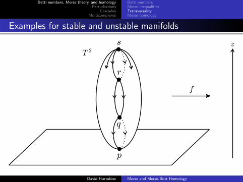
Examples for stable and unstable manifolds
S n
s
2
0
1
1¡
f x y z z( , , )=
David Hurtubise Morse and Morse-Bott Homology
Betti numbers, Morse theory, and homologyPerturbations
CascadesMulticomplexes
Betti numbersMorse inequalitiesTransversalityMorse homology
Examples for stable and unstable manifolds
f
Tz
2
p
q
r
s
David Hurtubise Morse and Morse-Bott Homology
Betti numbers, Morse theory, and homologyPerturbations
CascadesMulticomplexes
Betti numbersMorse inequalitiesTransversalityMorse homology
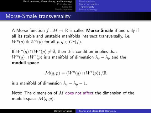
Morse-Smale transversality
A Morse function f : M → R is called Morse-Smale if and only ifall its stable and unstable manifolds intersect transversally, i.e.W u(q) t W s(p) for all p, q ∈ Cr(f).
If W u(q) ∩W s(p) 6= ∅, then this condition implies thatW u(q) ∩W s(p) is a manifold of dimension λq − λp and themoduli space
M(q, p) = (W u(q) ∩W s(p)) /R
is a manifold of dimension λq − λp − 1.
Note: The dimension of M does not affect the dimension of themoduli space M(q, p).
David Hurtubise Morse and Morse-Bott Homology

Betti numbers, Morse theory, and homologyPerturbations
CascadesMulticomplexes
Betti numbersMorse inequalitiesTransversalityMorse homology
A Morse-Smale function on a 2-torus
f
T
z2
p
q
r
s
David Hurtubise Morse and Morse-Bott Homology
Betti numbers, Morse theory, and homologyPerturbations
CascadesMulticomplexes
Betti numbersMorse inequalitiesTransversalityMorse homology
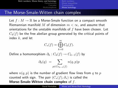
The Morse-Smale-Witten chain complex
Let f : M → R be a Morse-Smale function on a compact smoothRiemannian manifold M of dimension m < ∞, and assume thatorientations for the unstable manifolds of f have been chosen. LetCk(f) be the free abelian group generated by the critical points ofindex k, and let
C∗(f) =m⊕
k=0
Ck(f).
Define a homomorphism ∂k : Ck(f) → Ck−1(f) by
∂k(q) =∑
p∈Crk−1(f)
n(q, p)p
where n(q, p) is the number of gradient flow lines from q to pcounted with sign. The pair (C∗(f), ∂∗) is called theMorse-Smale-Witten chain complex of f .
David Hurtubise Morse and Morse-Bott Homology

Betti numbers, Morse theory, and homologyPerturbations
CascadesMulticomplexes
Betti numbersMorse inequalitiesTransversalityMorse homology
The height function on the 2-sphere
S n
s
2
0
1
1¡
f x y z z( , , )=
C2(f)∂2 //
OO≈
��
C1(f)OO≈
��
∂1 // C0(f)OO≈
��
// 0
< n >∂2 // < 0 >
∂1 // < s > // 0
David Hurtubise Morse and Morse-Bott Homology
Betti numbers, Morse theory, and homologyPerturbations
CascadesMulticomplexes
Betti numbersMorse inequalitiesTransversalityMorse homology
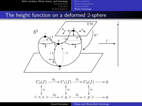
The height function on a deformed 2-sphere
f
S
z
2
p
q
r
s
T Ms
u
Eu
¡1+1
+1 ¡1
C2(f)∂2 //
OO≈
��
C1(f)OO≈
��
∂1 // C0(f)OO≈
��
// 0
< r, s >∂2 // < q >
∂1 // < p > // 0David Hurtubise Morse and Morse-Bott Homology

Betti numbers, Morse theory, and homologyPerturbations
CascadesMulticomplexes
Betti numbersMorse inequalitiesTransversalityMorse homology
The height function on a tilted 2-torus
f
z
p
q
r
s
T Mp
T Mq
T Mr
T Ms
+1
+1
+1
+1
¡1
¡1
¡1
¡1
T 2
C2(f)∂2 //
OO≈
��
C1(f)OO≈
��
∂1 // C0(f)OO≈
��
// 0
< s >∂2 // < q, r >
∂1 // < p > // 0David Hurtubise Morse and Morse-Bott Homology

Betti numbers, Morse theory, and homologyPerturbations
CascadesMulticomplexes
Betti numbersMorse inequalitiesTransversalityMorse homology
References for Morse homology
I Augustin Banyaga and David Hurtubise, Lectures on Morsehomology, Kluwer Texts in the Mathematical Sciences 29,Kluwer Academic Publishers Group, 2004.
I John Milnor, Lectures on the h-cobordism theorem,Princeton University Press, 1965.
I Liviu Nicolaescu, An Invitation to Morse Theory,Universitext, Springer 2007.
I Matthias Schwarz, Morse homology, Progress inMathematics 111, Birkhauser, 1993.
I Edward Witten, Supersymmetry and Morse theory, J.Differential Geom. 17 (1982), no. 4, 661–692.
David Hurtubise Morse and Morse-Bott Homology

Betti numbers, Morse theory, and homologyPerturbations
CascadesMulticomplexes
Betti numbersMorse inequalitiesTransversalityMorse homology
A Morse-Bott function on the 2-sphere
S
0
1
1
f x y z z( , , )= 2
2
B0
B2
n
s
Can we construct a chain complex for this function? a spectralsequence? a multicomplex?
David Hurtubise Morse and Morse-Bott Homology

Betti numbers, Morse theory, and homologyPerturbations
CascadesMulticomplexes
Generic perturbationsApplications of the perturbation approachA more explicit perturbationMorse-Bott inequalities
Generic perturbations
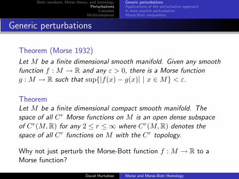
Theorem (Morse 1932)
Let M be a finite dimensional smooth manifold. Given any smoothfunction f : M → R and any ε > 0, there is a Morse functiong : M → R such that sup{|f(x)− g(x)| | x ∈ M} < ε.
TheoremLet M be a finite dimensional compact smooth manifold. Thespace of all Cr Morse functions on M is an open dense subspaceof Cr(M, R) for any 2 ≤ r ≤ ∞ where Cr(M, R) denotes thespace of all Cr functions on M with the Cr topology.
Why not just perturb the Morse-Bott function f : M → R to aMorse function?
David Hurtubise Morse and Morse-Bott Homology
Betti numbers, Morse theory, and homologyPerturbations
CascadesMulticomplexes
Generic perturbationsApplications of the perturbation approachA more explicit perturbationMorse-Bott inequalities
Generic perturbations
Theorem (Morse 1932)
Let M be a finite dimensional smooth manifold. Given any smoothfunction f : M → R and any ε > 0, there is a Morse functiong : M → R such that sup{|f(x)− g(x)| | x ∈ M} < ε.
TheoremLet M be a finite dimensional compact smooth manifold. Thespace of all Cr Morse functions on M is an open dense subspaceof Cr(M, R) for any 2 ≤ r ≤ ∞ where Cr(M, R) denotes thespace of all Cr functions on M with the Cr topology.
Why not just perturb the Morse-Bott function f : M → R to aMorse function?
David Hurtubise Morse and Morse-Bott Homology

Betti numbers, Morse theory, and homologyPerturbations
CascadesMulticomplexes
Generic perturbationsApplications of the perturbation approachA more explicit perturbationMorse-Bott inequalities
Fiber bundles and group actions
If π : E → B is a smooth fiber bundle with fiber F , and f is aMorse function on B, then f ◦ π is a Morse-Bott function withcritical submanifolds diffeomorphic to F .
F // E
π
��B
f // R
In particular, if G is a Lie group acting on M , then this might beuseful for studying equivariant homology.
M // EG×G M
π
��BG
f // R
David Hurtubise Morse and Morse-Bott Homology

Betti numbers, Morse theory, and homologyPerturbations
CascadesMulticomplexes
Generic perturbationsApplications of the perturbation approachA more explicit perturbationMorse-Bott inequalities
Fiber bundles and group actions
If π : E → B is a smooth fiber bundle with fiber F , and f is aMorse function on B, then f ◦ π is a Morse-Bott function withcritical submanifolds diffeomorphic to F .
F // E
π
��B
f // RIn particular, if G is a Lie group acting on M , then this might beuseful for studying equivariant homology.
M // EG×G M
π
��BG
f // RDavid Hurtubise Morse and Morse-Bott Homology

Betti numbers, Morse theory, and homologyPerturbations
CascadesMulticomplexes
Generic perturbationsApplications of the perturbation approachA more explicit perturbationMorse-Bott inequalities
Symplectic and Instanton Floer homology
I Andreas Floer, An instanton-invariant for 3-manifolds, Comm.Math. Phys. 118 (1988), no. 2, 215–240.
I Andreas Floer, Morse theory for Lagrangian intersections,Journal of Differential Geom 28 (1988), 513–547.
I Andreas Floer, Symplectic fixed points and holomorphicspheres, Comm. Math. Phys. 120 (1989), no. 4, 575–611.
Generalizations: Donaldson polynomials for 4-manifolds withboundary, knot homology groups, comparing the quantum cupproduct to the pair of pants product.
David Hurtubise Morse and Morse-Bott Homology

Betti numbers, Morse theory, and homologyPerturbations
CascadesMulticomplexes
Generic perturbationsApplications of the perturbation approachA more explicit perturbationMorse-Bott inequalities
An explicit perturbation of f : M → R
Let Tj be a small tubular neighborhood around each connectedcomponent Cj ⊆ Cr(f) for all j = 1, . . . , l. Pick a positive Morsefunction fj : Cj → R and extend fj to a function on Tj by makingfj constant in the direction normal to Cj for all j = 1, . . . , l.
Let Tj ⊂ Tj be a smaller tubular neighborhood of Cj with thesame coordinates as Tj , and let ρj be a smooth bump functionwhich is constant in the coordinates parallel to Cj , equal to 1 onTj , equal to 0 outside of Tj , and decreases on Tj − Tj as thecoordinates move away from Cj . For small ε > 0 (and a carefulchoice of the metric) this determines a Morse-Smale function
hε = f + ε
l∑j=1
ρjfj
.
David Hurtubise Morse and Morse-Bott Homology

Betti numbers, Morse theory, and homologyPerturbations
CascadesMulticomplexes
Generic perturbationsApplications of the perturbation approachA more explicit perturbationMorse-Bott inequalities
An explicit perturbation of f : M → R
Let Tj be a small tubular neighborhood around each connectedcomponent Cj ⊆ Cr(f) for all j = 1, . . . , l. Pick a positive Morsefunction fj : Cj → R and extend fj to a function on Tj by makingfj constant in the direction normal to Cj for all j = 1, . . . , l.
Let Tj ⊂ Tj be a smaller tubular neighborhood of Cj with thesame coordinates as Tj , and let ρj be a smooth bump functionwhich is constant in the coordinates parallel to Cj , equal to 1 onTj , equal to 0 outside of Tj , and decreases on Tj − Tj as thecoordinates move away from Cj .
For small ε > 0 (and a carefulchoice of the metric) this determines a Morse-Smale function
hε = f + ε
l∑j=1
ρjfj
.
David Hurtubise Morse and Morse-Bott Homology

Betti numbers, Morse theory, and homologyPerturbations
CascadesMulticomplexes
Generic perturbationsApplications of the perturbation approachA more explicit perturbationMorse-Bott inequalities
An explicit perturbation of f : M → R
Let Tj be a small tubular neighborhood around each connectedcomponent Cj ⊆ Cr(f) for all j = 1, . . . , l. Pick a positive Morsefunction fj : Cj → R and extend fj to a function on Tj by makingfj constant in the direction normal to Cj for all j = 1, . . . , l.
Let Tj ⊂ Tj be a smaller tubular neighborhood of Cj with thesame coordinates as Tj , and let ρj be a smooth bump functionwhich is constant in the coordinates parallel to Cj , equal to 1 onTj , equal to 0 outside of Tj , and decreases on Tj − Tj as thecoordinates move away from Cj . For small ε > 0 (and a carefulchoice of the metric) this determines a Morse-Smale function
hε = f + ε
l∑j=1
ρjfj
.
David Hurtubise Morse and Morse-Bott Homology

Betti numbers, Morse theory, and homologyPerturbations
CascadesMulticomplexes
Generic perturbationsApplications of the perturbation approachA more explicit perturbationMorse-Bott inequalities
Critical points of the perturbed function
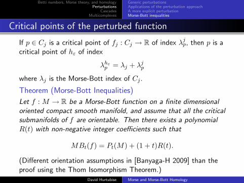
If p ∈ Cj is a critical point of fj : Cj → R of index λjp, then p is a
critical point of hε of index
λhεp = λj + λj
p
where λj is the Morse-Bott index of Cj .
Theorem (Morse-Bott Inequalities)
Let f : M → R be a Morse-Bott function on a finite dimensionaloriented compact smooth manifold, and assume that all the criticalsubmanifolds of f are orientable. Then there exists a polynomialR(t) with non-negative integer coefficients such that
MBt(f) = Pt(M) + (1 + t)R(t).
(Different orientation assumptions in [Banyaga-H 2009] than theproof using the Thom Isomorphism Theorem.)
David Hurtubise Morse and Morse-Bott Homology
Betti numbers, Morse theory, and homologyPerturbations
CascadesMulticomplexes
Generic perturbationsApplications of the perturbation approachA more explicit perturbationMorse-Bott inequalities
Critical points of the perturbed function
If p ∈ Cj is a critical point of fj : Cj → R of index λjp, then p is a
critical point of hε of index
λhεp = λj + λj
p
where λj is the Morse-Bott index of Cj .
Theorem (Morse-Bott Inequalities)
Let f : M → R be a Morse-Bott function on a finite dimensionaloriented compact smooth manifold, and assume that all the criticalsubmanifolds of f are orientable. Then there exists a polynomialR(t) with non-negative integer coefficients such that
MBt(f) = Pt(M) + (1 + t)R(t).
(Different orientation assumptions in [Banyaga-H 2009] than theproof using the Thom Isomorphism Theorem.)
David Hurtubise Morse and Morse-Bott Homology

Betti numbers, Morse theory, and homologyPerturbations
CascadesMulticomplexes
Generic perturbationsApplications of the perturbation approachA more explicit perturbationMorse-Bott inequalities
The idea behind the Banyaga-H proof
MBt(f) =l∑
j=1
Pt(Cj)tλj
=l∑
j=1
Mt(fj)− (1 + t)Rj(t)
tλj
=l∑
j=1
Mt(fj)tλj − (1 + t)l∑
j=1
Rj(t)tλj
= Mt(h)− (1 + t)l∑
j=1
Rj(t)tλj
= Pt(M) + (1 + t)Rh(t)− (1 + t)l∑
j=1
Rj(t)tλj
David Hurtubise Morse and Morse-Bott Homology

Betti numbers, Morse theory, and homologyPerturbations
CascadesMulticomplexes
Picture of a 3-cascadeExamples for the cascade chain complexApplications of the cascade approachCascades and perturbations
Cascades (Frauenfelder 2003 and Bourgeois 2002)
Let f : M → R be a Morse-Bott function and suppose
Cr(f) =l∐
j=1
Cj ,
where C1, . . . , Cl are disjoint connected critical submanifolds ofMorse-Bott index λ1, . . . , λl respectively. Let fj : Cj → R be aMorse function on the critical submanifold Cj for all j = 1, . . . , l.
DefinitionIf q ∈ Cj is a critical point of the Morse function fj : Cj → R forsome j = 1, . . . , l, then the total index of q, denoted λq, isdefined to be the sum of the Morse-Bott index of Cj and theMorse index of q relative to fj , i.e.
λq = λj + λjq.
David Hurtubise Morse and Morse-Bott Homology
Betti numbers, Morse theory, and homologyPerturbations
CascadesMulticomplexes
Picture of a 3-cascadeExamples for the cascade chain complexApplications of the cascade approachCascades and perturbations
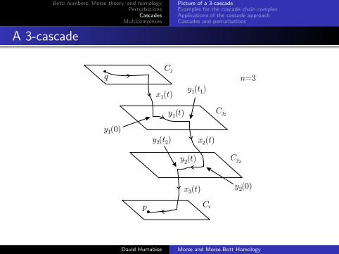
A 3-cascade
p
q
x t( )1
x t( )2
x t( )3
Cj
Ci
y t( )1
y t( )2
Cj1
Cj2
y t( )1 1
y t( )2 2
y (0)1
y (0)2
n=3
David Hurtubise Morse and Morse-Bott Homology

Betti numbers, Morse theory, and homologyPerturbations
CascadesMulticomplexes
Picture of a 3-cascadeExamples for the cascade chain complexApplications of the cascade approachCascades and perturbations
DefinitionDenote the space of flow lines from q to p with n cascades byW c
n(q, p), and denote the quotient of W cn(q, p) by the action of Rn
by Mcn(q, p) = W c
n(q, p)/Rn. The set of unparameterized flowlines with cascades from q to p is defined to be
Mc(q, p) =⋃
n∈Z+
Mcn(q, p)
where Mc0(q, p) = W c
0 (q, p)/R.
David Hurtubise Morse and Morse-Bott Homology

Betti numbers, Morse theory, and homologyPerturbations
CascadesMulticomplexes
Picture of a 3-cascadeExamples for the cascade chain complexApplications of the cascade approachCascades and perturbations
The Z2-cascade chain complex
Define the kth chain group Cck(f) to be the free abelian group
generated by the critical points of total index k of theMorse-Smale functions fj for all j = 1, . . . , l, and definenc(q, p; Z2) to be the number of flow lines with cascades betweena critical point q of total index k and a critical point p of totalindex k − 1 counted mod 2. Let
Cc∗(f)⊗ Z2 =
m⊕k=0
Cck(f)⊗ Z2
and define a homomorphism ∂ck : Cc
k(f)⊗ Z2 → Cck−1(f)⊗ Z2 by
∂ck(q) =
∑p∈Cr(fk−1)
nc(q, p; Z2)p.
The pair (Cc∗(f)⊗ Z2, ∂
c∗) is called the cascade chain complex
with Z2 coefficients.David Hurtubise Morse and Morse-Bott Homology

Betti numbers, Morse theory, and homologyPerturbations
CascadesMulticomplexes
Picture of a 3-cascadeExamples for the cascade chain complexApplications of the cascade approachCascades and perturbations
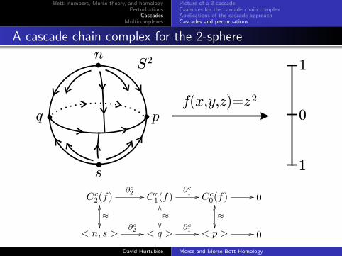
A cascade chain complex for the 2-sphere
S
0
1
1
2n
s
pqf x y z z( , , )= 2
Cc2(f)
∂c2 //
OO≈
��
Cc1(f)
OO≈
��
∂c1 // Cc
0(f)OO≈
��
// 0
< n, s >∂c2 // < q >
∂c1 // < p > // 0
David Hurtubise Morse and Morse-Bott Homology
Betti numbers, Morse theory, and homologyPerturbations
CascadesMulticomplexes
Picture of a 3-cascadeExamples for the cascade chain complexApplications of the cascade approachCascades and perturbations
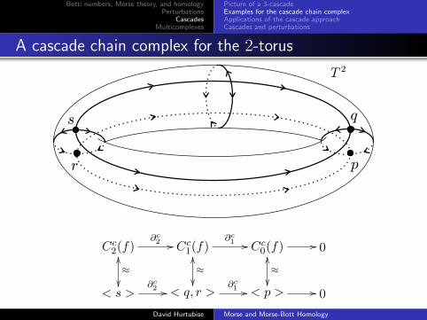
A cascade chain complex for the 2-torus
T 2
p
s
r
q
Cc2(f)
∂c2 //
OO≈
��
Cc1(f)
OO≈
��
∂c1 // Cc
0(f)OO≈
��
// 0
< s >∂c2 // < q, r >
∂c1 // < p > // 0
David Hurtubise Morse and Morse-Bott Homology

Betti numbers, Morse theory, and homologyPerturbations
CascadesMulticomplexes
Picture of a 3-cascadeExamples for the cascade chain complexApplications of the cascade approachCascades and perturbations
The Arnold-Givental conjecture
Let (M,ω) be a 2n-dimensional compact symplectic manifold,L ⊂ M a compact Lagrangian submanifold, and R ∈ Diff(M) anantisymplectic involution, i.e. R∗ω = −ω and R2 = id, whose fixedpoint set is L.Conjecture. Let Ht be a smooth family of Hamiltonian functionson M for 0 ≤ t ≤ 1 and denote by ΦH the time-1 map of the flowof the Hamiltonian vector field of Ht. If L intersects ΦH(L)transversally, then
#(L ∩ ΦH(L)) ≥n∑
k=0
bk(L; Z2).
Proved by Frauenfelder for a class of Lagrangians inMarsden-Weinstein quotients by letting H → 0 (2004).
David Hurtubise Morse and Morse-Bott Homology

Betti numbers, Morse theory, and homologyPerturbations
CascadesMulticomplexes
Picture of a 3-cascadeExamples for the cascade chain complexApplications of the cascade approachCascades and perturbations
The explicit perturbation of f : M → R
Let Tj be a small tubular neighborhood around each connectedcomponent Cj ⊆ Cr(f) for all j = 1, . . . , l. Pick a positive Morsefunction fj : Cj → R and extend fj to a function on Tj by makingfj constant in the direction normal to Cj for all j = 1, . . . , l.
Let Tj ⊂ Tj be a smaller tubular neighborhood of Cj with thesame coordinates as Tj , and let ρj be a smooth bump functionwhich is constant in the coordinates parallel to Cj , equal to 1 onTj , equal to 0 outside of Tj , and decreases on Tj − Tj as thecoordinates move away from Cj . For small ε > 0 (and a carefulchoice of the metric) this determines a Morse-Smale function
hε = f + ε
l∑j=1
ρjfj
.
David Hurtubise Morse and Morse-Bott Homology

Betti numbers, Morse theory, and homologyPerturbations
CascadesMulticomplexes
Picture of a 3-cascadeExamples for the cascade chain complexApplications of the cascade approachCascades and perturbations
A perturbed Morse-Bott function on the 2-sphere
S
0
1
1
2n
s
pqf x y z z( , , )= 2
C2(hε)∂2 //
OO≈
��
C1(hε)OO≈
��
∂1 // C0(hε)OO≈
��
// 0
< n, s >∂2 // < q >
∂1 // < p > // 0
David Hurtubise Morse and Morse-Bott Homology
Betti numbers, Morse theory, and homologyPerturbations
CascadesMulticomplexes
Picture of a 3-cascadeExamples for the cascade chain complexApplications of the cascade approachCascades and perturbations
A cascade chain complex for the 2-sphere
S
0
1
1
2n
s
pqf x y z z( , , )= 2
Cc2(f)
∂c2 //
OO≈
��
Cc1(f)
OO≈
��
∂c1 // Cc
0(f)OO≈
��
// 0
< n, s >∂c2 // < q >
∂c1 // < p > // 0
David Hurtubise Morse and Morse-Bott Homology

Betti numbers, Morse theory, and homologyPerturbations
CascadesMulticomplexes
Picture of a 3-cascadeExamples for the cascade chain complexApplications of the cascade approachCascades and perturbations
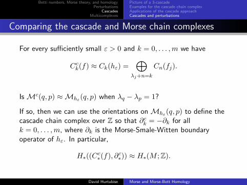
Comparing the cascade and Morse chain complexes
For every sufficiently small ε > 0 and k = 0, . . . ,m we have
Cck(f) ≈ Ck(hε) =
⊕λj+n=k
Cn(fj).
Is Mc(q, p) ≈Mhε(q, p) when λq − λp = 1?
If so, then we can use the orientations on Mhε(q, p) to define thecascade chain complex over Z so that ∂c
k = −∂k for allk = 0, . . . ,m, where ∂k is the Morse-Smale-Witten boundaryoperator of hε. In particular,
H∗((Cc∗(f), ∂c
∗)) ≈ H∗(M ; Z).
David Hurtubise Morse and Morse-Bott Homology

Betti numbers, Morse theory, and homologyPerturbations
CascadesMulticomplexes
Picture of a 3-cascadeExamples for the cascade chain complexApplications of the cascade approachCascades and perturbations
Comparing the cascade and Morse chain complexes
For every sufficiently small ε > 0 and k = 0, . . . ,m we have
Cck(f) ≈ Ck(hε) =
⊕λj+n=k
Cn(fj).
Is Mc(q, p) ≈Mhε(q, p) when λq − λp = 1?
If so, then we can use the orientations on Mhε(q, p) to define thecascade chain complex over Z so that ∂c
k = −∂k for allk = 0, . . . ,m, where ∂k is the Morse-Smale-Witten boundaryoperator of hε. In particular,
H∗((Cc∗(f), ∂c
∗)) ≈ H∗(M ; Z).
David Hurtubise Morse and Morse-Bott Homology

Betti numbers, Morse theory, and homologyPerturbations
CascadesMulticomplexes
Picture of a 3-cascadeExamples for the cascade chain complexApplications of the cascade approachCascades and perturbations
Theorem (Banyaga-H 2013)
Assume that f satisfies the Morse-Bott-Smale transversalitycondition with respect to the Riemannian metric g on M ,fk : Ck → R satisfies the Morse-Smale transversality conditionwith respect to the restriction of g to Ck for all k = 1, . . . , l, andthe unstable and stable manifolds W u
fj(q) and W s
fi(p) are
transverse to the beginning and endpoint maps.
1. When n = 0, 1 the set Mcn(q, p) is either empty or a smooth
manifold without boundary.
2. For n > 1 the set Mcn(q, p) is either empty or a smooth
manifold with corners.
3. The set Mc(q, p) is either empty or a smooth manifoldwithout boundary.
In each case the dimension of the manifold is λq − λp − 1. Theabove manifolds are orientable when M and Ck are orientable.
David Hurtubise Morse and Morse-Bott Homology
Betti numbers, Morse theory, and homologyPerturbations
CascadesMulticomplexes
Picture of a 3-cascadeExamples for the cascade chain complexApplications of the cascade approachCascades and perturbations
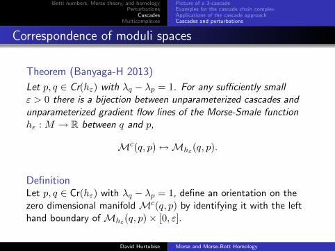
Correspondence of moduli spaces
Theorem (Banyaga-H 2013)
Let p, q ∈ Cr(hε) with λq − λp = 1. For any sufficiently smallε > 0 there is a bijection between unparameterized cascades andunparameterized gradient flow lines of the Morse-Smale functionhε : M → R between q and p,
Mc(q, p) ↔Mhε(q, p).
DefinitionLet p, q ∈ Cr(hε) with λq − λp = 1, define an orientation on thezero dimensional manifold Mc(q, p) by identifying it with the lefthand boundary of Mhε(q, p)× [0, ε].
David Hurtubise Morse and Morse-Bott Homology

Betti numbers, Morse theory, and homologyPerturbations
CascadesMulticomplexes
Picture of a 3-cascadeExamples for the cascade chain complexApplications of the cascade approachCascades and perturbations
Main idea: The Exchange Lemma
x t( )k y t( )k k
Bk
Sk
qk
u
vw
"x t( )k+1
x t( )k+1
rk+1
"x t( )k
y (0)k
rk~r
k
David Hurtubise Morse and Morse-Bott Homology
Betti numbers, Morse theory, and homologyPerturbations
CascadesMulticomplexes
Picture of a 3-cascadeExamples for the cascade chain complexApplications of the cascade approachCascades and perturbations
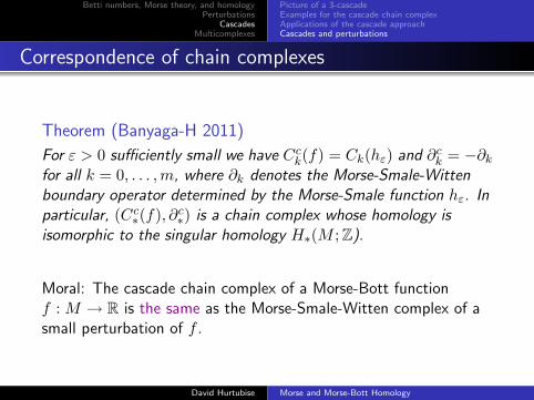
Correspondence of chain complexes
Theorem (Banyaga-H 2011)
For ε > 0 sufficiently small we have Cck(f) = Ck(hε) and ∂c
k = −∂k
for all k = 0, . . . ,m, where ∂k denotes the Morse-Smale-Wittenboundary operator determined by the Morse-Smale function hε. Inparticular, (Cc
∗(f), ∂c∗) is a chain complex whose homology is
isomorphic to the singular homology H∗(M ; Z).
Moral: The cascade chain complex of a Morse-Bott functionf : M → R is the same as the Morse-Smale-Witten complex of asmall perturbation of f .
David Hurtubise Morse and Morse-Bott Homology

Betti numbers, Morse theory, and homologyPerturbations
CascadesMulticomplexes
Definition and assemblyMulticomplexes and spectral sequencesThe Morse-Bott-Smale multicomplexReferences
MulticomplexesLet R be a principal ideal domain. A first quadrant multicomplexX is a bigraded R-module {Xp,q}p,q∈Z+ with differentials
di : Xp,q → Xp−i,q+i−1 for all i = 0, 1, . . .
that satisfy ∑i+j=n
didj = 0 for all n.
A first quadrant multicomplex can be assembled to form a filteredchain complex ((CX)∗, ∂) by summing along the diagonals, i.e.
(CX)n ≡⊕
p+q=n
Xp,q and Fs(CX)n ≡⊕
p+q=np≤s
Xp,q
and ∂n = d0 ⊕ · · · ⊕ dn for all n ∈ Z+. The above relations thenimply that ∂n ◦ ∂n+1 = 0 and ∂n(Fs(CX)∗) ⊆ Fs(CX)∗.
David Hurtubise Morse and Morse-Bott Homology

Betti numbers, Morse theory, and homologyPerturbations
CascadesMulticomplexes
Definition and assemblyMulticomplexes and spectral sequencesThe Morse-Bott-Smale multicomplexReferences
......
......
X0,3
d0
��
X1,3
d0
��
d1oo X2,3
d0
��
d1oo X3,3
d0
��
d1oo · · ·
X0,2
d0
��
X1,2
d0
��
d1oo X2,2
d0
��
d1ood2RRRRR
RR
iiRRRRRRRR
X3,2
d0
��
d1ood2RRRRR
RR
iiRRRRRRRR
· · ·
X0,1
d0
��
X1,1
d0
��
d1oo X2,1
d0
��
d1ood2RRRRR
RR
iiRRRRRRRR
X3,1
d0
��
d1ood2RRRRR
RR
iiRRRRRRRRd3
ff
· · ·
X0,0 X1,0d1oo X2,0
d1ood2RRRRR
RR
iiRRRRRRRR
X3,0d1oo
d2RRRRRRR
iiRRRRRRRRd3
ff
· · ·
A bicomplex has two filtrations, but a general multicomplex onlyhas one filtration.
David Hurtubise Morse and Morse-Bott Homology

Betti numbers, Morse theory, and homologyPerturbations
CascadesMulticomplexes
Definition and assemblyMulticomplexes and spectral sequencesThe Morse-Bott-Smale multicomplexReferences
· · · X3,0d0 //
d1
$$JJJJJJJJJ
d2
7777
77
��777
7777
7d3
��
0
· · · X2,1
⊕
d0 //
d1
$$JJJJJJJJJ
d2
7777
77
��777
7777
7
X2,0
⊕
d0 //
d1
$$JJJJJJJJJ
d2
7777
77
��777
7777
7
0
· · · X1,2
⊕
d0 //
d1
$$JJJJJJJJJX1,1
⊕
d0 //
d1
$$JJJJJJJJJX1,0
⊕
d0 //
d1
$$JJJJJJJJJ 0
· · · X0,3
⊕
d0 // X0,2
⊕
d0 // X0,1
⊕
d0 // X0,0
⊕
d0 // 0
· · · (CX)3
‖
∂3 // (CX)2
‖
∂2 // (CX)1
‖
∂1 // (CX)0
‖
∂0 // 0
‖
David Hurtubise Morse and Morse-Bott Homology

Betti numbers, Morse theory, and homologyPerturbations
CascadesMulticomplexes
Definition and assemblyMulticomplexes and spectral sequencesThe Morse-Bott-Smale multicomplexReferences
The bigraded module associated to the filtration
Fs(CX)n ≡⊕
p+q=np≤s
Xp,q
isG((CX)∗)s,t = Fs(CX)s+t/Fs−1(CX)s+t ≈ Xs,t
for all s, t ∈ Z+, and the E1 term of the associated spectralsequence is given by
E1s,t = Z1
s,t
/(Z0
s−1,t+1 + ∂Z0s,t+1
)where
Z1s,t = {c ∈ Fs(CX)s+t| ∂c ∈ Fs−1(CX)s+t−1}
Z0s,t = {c ∈ Fs(CX)s+t| ∂c ∈ Fs(CX)s+t−1} = Fs(CX)s+t.
David Hurtubise Morse and Morse-Bott Homology

Betti numbers, Morse theory, and homologyPerturbations
CascadesMulticomplexes
Definition and assemblyMulticomplexes and spectral sequencesThe Morse-Bott-Smale multicomplexReferences
E1s,t and d1 are induced from d0 and d1
TheoremLet ({Xp,q}p,q∈Z+ , {di}i∈Z+) be a first quadrant multicomplex and((CX)∗, ∂) the associated assembled chain complex. Then the E1
term of the spectral sequence associated to the filtration of (CX)∗determined by the restriction p ≤ s is given byE1
s,t ≈ Hs+t(Xs,∗, d0) where (Xs,∗, d0) denotes the following chaincomplex.
· · · d0 // Xs,3d0 // Xs,2
d0 // Xs,1d0 // Xs,0
d0 // 0
Moreover, the d1 differential on the E1 term of the spectralsequence is induced from the homomorphism d1 in themulticomplex.
David Hurtubise Morse and Morse-Bott Homology
Betti numbers, Morse theory, and homologyPerturbations
CascadesMulticomplexes
Definition and assemblyMulticomplexes and spectral sequencesThe Morse-Bott-Smale multicomplexReferences
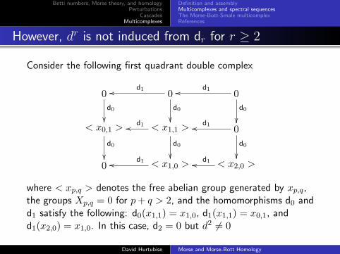
However, dr is not induced from dr for r ≥ 2
Consider the following first quadrant double complex
0d0
��
0d0
��
d1oo 0d0
��
d1oo
< x0,1 >
d0
��
< x1,1 >
d0
��
d1oo 0d0
��
d1oo
0 < x1,0 >d1oo < x2,0 >d1oo
where < xp,q > denotes the free abelian group generated by xp,q,the groups Xp,q = 0 for p + q > 2, and the homomorphisms d0 andd1 satisfy the following: d0(x1,1) = x1,0, d1(x1,1) = x0,1, andd1(x2,0) = x1,0. In this case, d2 = 0 but d2 6= 0
David Hurtubise Morse and Morse-Bott Homology

Betti numbers, Morse theory, and homologyPerturbations
CascadesMulticomplexes
Definition and assemblyMulticomplexes and spectral sequencesThe Morse-Bott-Smale multicomplexReferences
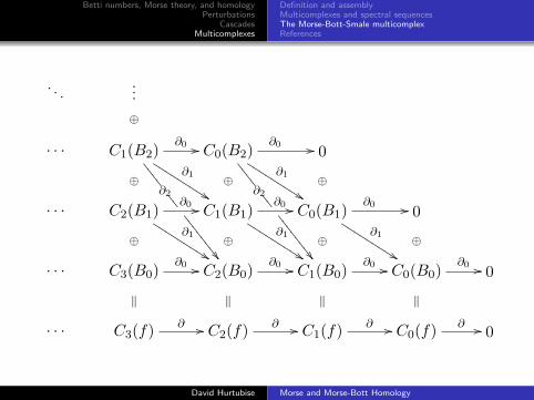
The Morse-Bott-Smale multicomplex
Let Cp(Bi) be the group of “p-dimensional chains” in the criticalsubmanifolds of index i. Assume that f : M → R is aMorse-Bott-Smale function and the manifold M , the criticalsubmanifolds, and their negative normal bundles are all orientable.
If σ : P → Bi is a singular Cp-space in S∞p (Bi), then for anyj = 1, . . . , i composing the projection map π2 onto the secondcomponent of P ×Bi M(Bi, Bi−j) with the endpoint map∂+ : M(Bi, Bi−j) → Bi−j gives a map
P ×Bi M(Bi, Bi−j)π2−→M(Bi, Bi−j)
∂+−→ Bi−j .
David Hurtubise Morse and Morse-Bott Homology
Betti numbers, Morse theory, and homologyPerturbations
CascadesMulticomplexes
Definition and assemblyMulticomplexes and spectral sequencesThe Morse-Bott-Smale multicomplexReferences
. . ....
· · · C1(B2)
⊕
∂0 //
∂1
%%KKKKKKKKK
∂2
8888
88
��888
8888
8
C0(B2)∂0 //
∂1
%%KKKKKKKKK
∂2
8888
88
��888
8888
8
0
· · · C2(B1)
⊕
∂0 //
∂1
%%KKKKKKKKKC1(B1)
⊕
∂0 //
∂1
%%KKKKKKKKKC0(B1)
⊕
∂0 //
∂1
%%KKKKKKKKK 0
· · · C3(B0)
⊕
∂0 // C2(B0)
⊕
∂0 // C1(B0)
⊕
∂0 // C0(B0)
⊕
∂0 // 0
· · · C3(f)
‖
∂ // C2(f)
‖
∂ // C1(f)
‖
∂ // C0(f)
‖
∂ // 0
David Hurtubise Morse and Morse-Bott Homology

Betti numbers, Morse theory, and homologyPerturbations
CascadesMulticomplexes
Definition and assemblyMulticomplexes and spectral sequencesThe Morse-Bott-Smale multicomplexReferences
The Morse-Bott Homology Theorem
Theorem (Banyaga-H 2010)
The homology of the Morse-Bott-Smale multicomplex (C∗(f), ∂)is independent of the Morse-Bott-Smale function f : M → R.Therefore,
H∗(C∗(f), ∂) ≈ H∗(M ; Z).
Note: If f is constant, then (C∗(f), ∂) is the chain complex ofsingular N -cube chains. If f is Morse-Smale, then (C∗(f), ∂) isthe Morse-Smale-Witten chain complex. This gives a new proof ofthe Morse Homology Theorem.
David Hurtubise Morse and Morse-Bott Homology

Betti numbers, Morse theory, and homologyPerturbations
CascadesMulticomplexes
Definition and assemblyMulticomplexes and spectral sequencesThe Morse-Bott-Smale multicomplexReferences
References
I David Austin and Peter Braam, Morse-Bott theory andequivariant cohomology, The Floer memorial volume,Progr. Math. 133 (1995), 123–183.
I David Austin and Peter Braam, Equivariant Floer theory andgluing Donaldson polynomials, Topology 35 (1996), no. 1,167–200.
I Augustin Banyaga and David Hurtubise, A proof of theMorse-Bott Lemma, Expo. Math. 22, no. 4, 365–373, 2004.
I Augustin Banyaga and David Hurtubise, Lectures on Morsehomology, Kluwer Texts in the Mathematical Sciences 29,Springer 2004.
I Augustin Banyaga and David Hurtubise, The Morse-Bottinequalities via a dynamical systems approach, Ergodic TheoryDynam. Systems 29 (2009), no. 6, 1693–1703.
David Hurtubise Morse and Morse-Bott Homology

Betti numbers, Morse theory, and homologyPerturbations
CascadesMulticomplexes
Definition and assemblyMulticomplexes and spectral sequencesThe Morse-Bott-Smale multicomplexReferences
References
I Augustin Banyaga and David Hurtubise, Morse-Botthomology, Trans. Amer. Math. Soc. 362 (2010), no. 8,3997–4043.
I Augustin Banyaga and David Hurtubise, Cascades andperturbed Morse-Bott functions, Algebr. Geom. Topol. 13(2013), 237-275.
I Frederic Bourgeois and Alexandru Oancea, Symplectichomology, autonomous Hamiltonians, and Morse-Bott modulispaces, Duke Math. J. 146 (2009), no. 1, 74–174.
I Frederic Bourgeois and Alexandru Oancea, An exact sequencefor contact and symplectic homology, Invent. Math. 179(2009), no. 3, 611–680.
I Andreas Floer, An instanton-invariant for 3-manifolds, Comm.Math. Phys. 118 (1988), no. 2, 215–240.
David Hurtubise Morse and Morse-Bott Homology

Betti numbers, Morse theory, and homologyPerturbations
CascadesMulticomplexes
Definition and assemblyMulticomplexes and spectral sequencesThe Morse-Bott-Smale multicomplexReferences
References
I Andreas Floer, An instanton-invariant for 3-manifolds, Comm.Math. Phys. 118 (1988), no. 2, 215–240.
I Andreas Floer, Instanton homology, surgery, and knots,Geometry of low-dimensional manifolds, London Math.Soc. Lecture Note Ser. 150 (1990), 97–114.
I Andreas Floer, Morse theory for Lagrangian intersections,Journal of Differential Geom 28 (1988), 513–547.
I Andreas Floer, Witten’s complex and infinite-dimensionalMorse theory, J. Differential Geom. 30 (1989), no. 1,207–221.
I Urs Frauenfelder, The Arnold-Givental conjecture andmoment Floer homology, Int. Math. Res. Not. 2004, no. 42,2179-2269.
David Hurtubise Morse and Morse-Bott Homology

Betti numbers, Morse theory, and homologyPerturbations
CascadesMulticomplexes
Definition and assemblyMulticomplexes and spectral sequencesThe Morse-Bott-Smale multicomplexReferences
References
I Kenji Fukaya, Floer homology of connected sum of homology3-spheres, Topology 35 (1996), no. 1, 89–136.
I David Hurtubise, Multicomplexes and spectral sequences, J.Algebra Appl. 9 (2010), no. 4, 519–530.
I David Hurtubise, Three approaches to Morse-Bott homology,Afr. Diaspora J. Math. 14 (2012), no. 2, 145–177.
I Jean-Pierre Meyer, Acyclic models for multicomplexes, DukeMath. J. 45 (1978), no. 1, 67-85.
I Liviu Nicolaescu, An Invitation to Morse Theory,Universitext, Springer 2007.
David Hurtubise Morse and Morse-Bott Homology

Betti numbers, Morse theory, and homologyPerturbations
CascadesMulticomplexes
Definition and assemblyMulticomplexes and spectral sequencesThe Morse-Bott-Smale multicomplexReferences
References
I Yongbin Ruan and Gang Tian, Bott-type symplectic Floercohomology and its multiplication structures, Math. Res.Lett. 2 (1995), no. 2, 203–219.
I Jan Swoboda, Morse homology for the Yang-Mills gradientflow, arXiv:1103.0845v1, 2011.
I Gang Liu and Gang Tian, On the equivalence of multiplicativestructures in Floer homology and quantum homology, ActaMath. Sin. 15 (1999), no. 1, 53–80.
I Joa Weber, The Morse-Witten complex via dynamicalsystems, Expo. Math. 24 (2006), no. 2, 127–159.
I Edward Witten. Supersymmetry and Morse theory, J.Differential Geom. 17 (1982), no. 4, 661–692 (1983).
David Hurtubise Morse and Morse-Bott Homology

Betti numbers, Morse theory, and homologyPerturbations
CascadesMulticomplexes
Definition and assemblyMulticomplexes and spectral sequencesThe Morse-Bott-Smale multicomplexReferences
The Chern-Simons functional
Let P → N be a (trivial) principal SU(2)-bundle over an orientedclosed 3-manifold N , and let A be the space of connections on P .Define CS : A → R by
CS(A) =1
4π2
∫M
tr(12A ∧ dA +
13A ∧A ∧A).
The above functional descends to a function cs : A/G → R/Zwhose critical points are gauge equivalence classes of flatconnections. Extending everything to P × R → N × R, thegradient flow equation becomes the instanton equation
F + ∗F = 0,
where F denotes the curvature and ∗ is the Hodge star operator.
David Hurtubise Morse and Morse-Bott Homology

Betti numbers, Morse theory, and homologyPerturbations
CascadesMulticomplexes
Definition and assemblyMulticomplexes and spectral sequencesThe Morse-Bott-Smale multicomplexReferences
Instanton homology
Andreas Floer, An instanton-invariant for 3-manifolds, Comm.Math. Phys. 118 (1988), no. 2, 215–240.
Theorem. When N is a homology 3-sphere the Chern-Simonsfunctional can be perturbed so that it has discrete critical pointsand defines Z8-graded homology groups I∗(N) analogous to theMorse homology groups.
Generalizations: Donaldson polynomials for 4-manifolds withboundary, knot homology groups
David Hurtubise Morse and Morse-Bott Homology

Betti numbers, Morse theory, and homologyPerturbations
CascadesMulticomplexes
Definition and assemblyMulticomplexes and spectral sequencesThe Morse-Bott-Smale multicomplexReferences
The symplectic action functional
Let (M,ω) be a closed symplectic manifold and S1 = R/Z. Atime-dependent Hamiltonian H : M × S1 → R determines atime-dependent vector field XH by
ω(XH(x, t), v) = v(H)(x, t) for v ∈ TxM.
Let L(M) be the space of free contractible loops on M and
L(M) = {(x, u)|x ∈ L(M), u : D2 → M such that u(e2πit) = x(t)}/ ∼
its universal cover with covering group π2(M). The symplecticaction functional aH : L(M) → R is defined by
aH((x, u)) =∫
D2
u∗ω +∫ 1
0H(x(t), t) dt.
David Hurtubise Morse and Morse-Bott Homology

Betti numbers, Morse theory, and homologyPerturbations
CascadesMulticomplexes
Definition and assemblyMulticomplexes and spectral sequencesThe Morse-Bott-Smale multicomplexReferences
The Arnold conjecture
Andreas Floer, Symplectic fixed points and holomorphic spheres,Comm. Math. Phys. 120 (1989), no. 4, 575–611.
Theorem. Let (P, ω) be a compact symplectic manifold. If Iω andIc are proportional, then the fixed point set of every exactdiffeomorphism of (P, ω) satisfies the Morse inequalities withrespect to any coefficient ring whenever it is nondegenerate.
Generalizations: Allowing H to be degenerate (e.g. H = 0) leadsto critical submanifolds and Morse-Bott homology.
David Hurtubise Morse and Morse-Bott Homology

Betti numbers, Morse theory, and homologyPerturbations
CascadesMulticomplexes
Definition and assemblyMulticomplexes and spectral sequencesThe Morse-Bott-Smale multicomplexReferences
The Yang-Mills gradient flow
Let (Σ, g) be a closed oriented Riemann surface, G a compact Liegroup, g its Lie algebra, and P a principal G-bundle over Σ. Pickan ad-invariant inner product on g, let A(P ) denote the affinespace of g-valued connection 1-forms on P , and defineYM : A(P ) → R by
YM(A) =∫
ΣFA ∧ ∗FA
where FA = dA + 12 [A ∧A] is the curvature of A.
The Yang-Mills function is a Morse-Bott function studied byAtiyah-Bott and by Swoboda (2011) using cascades.
David Hurtubise Morse and Morse-Bott Homology

Betti numbers, Morse theory, and homologyPerturbations
CascadesMulticomplexes
Definition and assemblyMulticomplexes and spectral sequencesThe Morse-Bott-Smale multicomplexReferences
Closed Reeb orbits
Let M be a compact, orientable manifold of dimension 2n− 1 withcontact form α. The Reeb vector field Rα associated to thecontact form α is characterized by
dα(Rα,−) = 0α(Rα) = 1.
Closed trajectories of the Reeb vector field are critical points of theaction functional A : C∞(S1,M) → R
A(γ) =∫
γα.
Lemma. For any contact structure ξ on M , there exists a contactform α for ξ such that all closed orbits of Rα are nondegenerate.
David Hurtubise Morse and Morse-Bott Homology
Betti numbers, Morse theory, and homologyPerturbations
CascadesMulticomplexes
Definition and assemblyMulticomplexes and spectral sequencesThe Morse-Bott-Smale multicomplexReferences
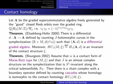
Contact homology
Let A be the graded supercommutative algebra freely generated bythe “good” closed Reeb orbits over the graded ringQ[H2(M ; Z)/R], i.e. γ1γ2 = (−1)|γ1||γ2|γ2γ1.
Theorem. (Eliashberg-Hofer 2000) There is a differentiald : A → A defined by counting J-holomorphic curves in thesymplectization (R×M,d(etα)) such that (A, d) is a differential
graded algebra. Moreover, HC∗(M, ξ) def= H∗(A, d) is an invariantof the contact structure ξ.
Theorem. (Bourgeois 2002) Assume that α is a contact form ofMorse-Bott type for (M, ξ) and that J is an almost complexstructure on the symplectization that is S1-invariant along thecritical submanifolds NT . Then there is a chain complex with aboundary operator defined by counting cascades whose homologyis isomorphic to the contact homology HC∗(M, ξ).
David Hurtubise Morse and Morse-Bott Homology

Betti numbers, Morse theory, and homologyPerturbations
CascadesMulticomplexes
Definition and assemblyMulticomplexes and spectral sequencesThe Morse-Bott-Smale multicomplexReferences
Viterbo’s symplectic homology
DefinitionA compact symplectic manifold (W,ω) has contact typeboundary if and only if there exists a vector field X defined in aneighborhood of M = ∂W transverse and pointing outward alongM such that LXω = ω.
In this case, λ = ω(X, ·)|M is a contact form on M , and thesymplectic homology of W combines the 1-periodic orbits of aHamiltonian on W with the Reeb orbits on M = ∂W .
Bourgeois and Oancea have defined the cascade chain complex fora time-independent Hamiltonian on W whose 1-periodic orbits aretransversally nondegenerate (2009). They have also proved thatthere is an exact sequence relating the symplectic homology groupsof W with the linearized contact homology groups of M (2009).
David Hurtubise Morse and Morse-Bott Homology
Betti numbers, Morse theory, and homologyPerturbations
CascadesMulticomplexes
Definition and assemblyMulticomplexes and spectral sequencesThe Morse-Bott-Smale multicomplexReferences
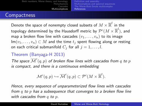
Compactness
Denote the space of nonempty closed subsets of M × Rlin the
topology determined by the Hausdorff metric by Pc(M × Rl), andmap a broken flow line with cascades (v1, . . . , vn) to its imageIm(v1, . . . , vn) ⊂ M and the time tj spent flowing along or restingon each critical submanifold Cj for all j = 1, . . . , l.
Theorem (Banyaga-H 2013)
The space Mc(q, p) of broken flow lines with cascades from q to pis compact, and there is a continuous embedding
Mc(q, p) ↪→Mc(q, p) ⊂ Pc(M × Rl).
Hence, every sequence of unparameterized flow lines with cascadesfrom q to p has a subsequence that converges to a broken flow linewith cascades from q to p.
David Hurtubise Morse and Morse-Bott Homology


![Stratified Morse Theory: Past and Present › Massey › Massey_preprints › ... · Theory [15] and Morse Theory and Intersection Homology Theory [14], which contained announcements](https://img.dokumen.tips/doc/110x75/5f030ea97e708231d4075280/stratiied-morse-theory-past-and-a-massey-a-masseypreprints-a-theory.jpg)
![Contents · This geometric theory developed further in the intersection homology and strati ed Morse the-ory of Goresky & MacPherson in [GM1], [GM2], and [GM3]. Their work continues](https://img.dokumen.tips/doc/110x75/5f0d0e867e708231d43876dd/this-geometric-theory-developed-further-in-the-intersection-homology-and-strati.jpg)


