1

The calculation of atomic and molecular spin-orbit coupling matrix

elements

Millard H. Alexander

CONTENTS

I. Introduction 1

II. Atoms 2

A. p1 electron occupancy 2

1. Transformation from definite-m to Cartesian basis: Fundamentals 3

2. Full (coupled) transformation to the Cartesian basis 5

3. Decoupled transformation to the Cartesian basis 5

B. p5 electron occupancy 8

C. p2 electron occupancy 12

1. Spin-orbit coupling within the 3P state 13

2. Spin-orbit coupling between the 3P and 1D states 17

D. Symmetry blocking 21

E. p4 electron occupancy 23

1. Spin-orbit coupling within the 3P state 23

References 23

I. INTRODUCTION

We write the electronic Hamiltonian as Hel(~r, ~R), where ~r and ~R denote, collectively,

the positions of the electrons and nuclei, respectively. This operator includes the kinetic

energy of the electrons and all electron-nuclei and electron-electron Coulomb interactions,

but neglects the much weaker interaction between the magnetic moments generated by the

orbital motion and spin of the electrons. The spin-orbit Hamiltonian for an N -electron

2

system can be written as

Hso =∑

i

ai~li · ~si =∑

i

ai (lxisxi

+ lyisyi + lziszi) =∑

i

ai[

lziszi +12(li+si− + li−si+)

]

Here ai is a one-electron operator which depends on the radial part of the electronic wave-

function. [1]

In this Chapter we shall explore the determination of the matrix of the spin-orbit Hamil-

tonian for several atomic and molecular systems, and make reference to Molpro input files

for the calculation of expectation value of a.

II. ATOMS

A. p1 electron occupancy

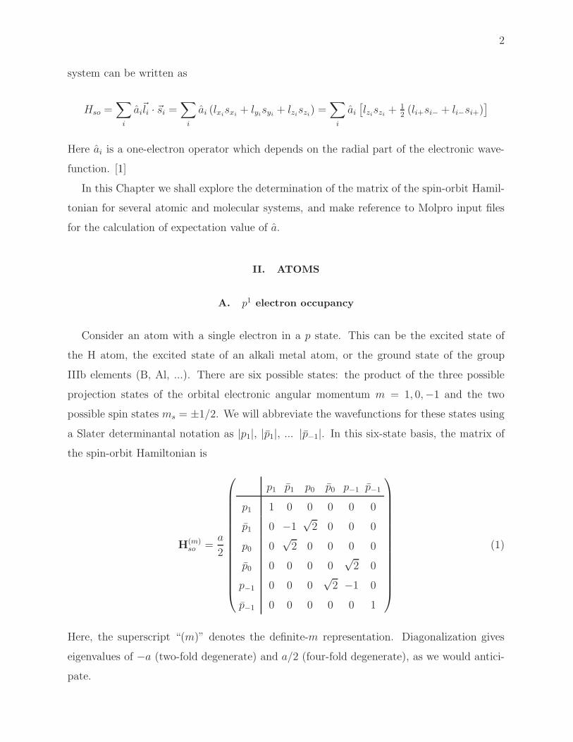
Consider an atom with a single electron in a p state. This can be the excited state of

the H atom, the excited state of an alkali metal atom, or the ground state of the group

IIIb elements (B, Al, ...). There are six possible states: the product of the three possible

projection states of the orbital electronic angular momentum m = 1, 0,−1 and the two

possible spin states ms = ±1/2. We will abbreviate the wavefunctions for these states using

a Slater determinantal notation as |p1|, |p1|, ... |p−1|. In this six-state basis, the matrix of

the spin-orbit Hamiltonian is

H(m)so =

a

2

p1 p1 p0 p0 p−1 p−1

p1 1 0 0 0 0 0

p1 0 −1√2 0 0 0

p0 0√2 0 0 0 0

p0 0 0 0 0√2 0

p−1 0 0 0√2 −1 0

p−1 0 0 0 0 0 1

(1)

Here, the superscript “(m)” denotes the definite-m representation. Diagonalization gives

eigenvalues of −a (two-fold degenerate) and a/2 (four-fold degenerate), as we would antici-

pate.

3

1. Transformation from definite-m to Cartesian basis: Fundamentals

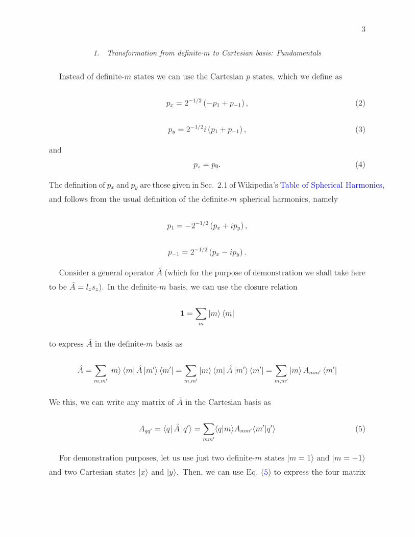
Instead of definite-m states we can use the Cartesian p states, which we define as

px = 2−1/2 (−p1 + p−1) , (2)

py = 2−1/2i (p1 + p−1) , (3)

and

pz = p0. (4)

The definition of px and py are those given in Sec. 2.1 of Wikipedia’s Table of Spherical Harmonics,

and follows from the usual definition of the definite-m spherical harmonics, namely

p1 = −2−1/2 (px + ipy) ,

p−1 = 2−1/2 (px − ipy) .

Consider a general operator A (which for the purpose of demonstration we shall take here

to be A = lzsz). In the definite-m basis, we can use the closure relation

1 =∑

m

|m〉 〈m|

to express A in the definite-m basis as

A =∑

m,m′

|m〉 〈m| A |m′〉 〈m′| =∑

m,m′

|m〉 〈m| A |m′〉 〈m′| =∑

m,m′

|m〉Amm′ 〈m′|

We this, we can write any matrix of A in the Cartesian basis as

Aqq′ = 〈q| A |q′〉 =∑

mm′

〈q|m〉Amm′〈m′|q′〉 (5)

For demonstration purposes, let us use just two definite-m states |m = 1〉 and |m = −1〉and two Cartesian states |x〉 and |y〉. Then, we can use Eq. (5) to express the four matrix

4

elements of the 2× 2 matrix of A in the Cartesian basis as follows:

Axx = 〈x|1〉A11〈1|x〉+ 〈x| − 1〉A−1,−1〈−1|x〉+ 〈x|1〉A1,−1〈−1|x〉+ 〈x| − 1〉A−1,1〈1|x〉

Axy = 〈x|1〉A11〈1|y〉+ 〈x| − 1〉A−1,−1〈−1|y〉+ 〈x|1〉A1,−1〈−1|y〉+ 〈x| − 1〉A−1,1〈1|y〉

Ayx = 〈y|1〉A11〈1|x〉+ 〈y| − 1〉A−1,−1〈−1|x〉+ 〈y|1〉A1,−1〈−1|x〉+ 〈y| − 1〉A−1,1〈1|x〉

Axy = 〈y|1〉A11〈1|y〉+ 〈y| − 1〉A−1,−1〈−1|y〉+ 〈y|1〉A1,−1〈−1|y〉+ 〈y| − 1〉A−1,1〈1|y〉

We can rewrite these four equations in matrix notation as

Axx Axy

Ayx Ayy

=

〈x| 1〉 〈x| −1〉〈y| 1〉 〈y| −1〉

A11 A1−1

A−11 A−1−1

〈1| x〉 〈1| y〉〈−1| x〉 〈−1| y〉

(6)

We now define a matrix T , which transforms from the definite-m to the Cartesian basis, as

Tjk ≡ 〈qj | mk〉 (7)

We also know that in general any matrix element and its transpose satisfy the equality

〈j|k〉 = 〈k|j〉∗

then Eq. (6) can be written as

A(q) = TA

(m)T

† (8)

where the Hermitian adjoint of a matrix is the complex conjugate of the transpose, namely

T† = (TT )∗.

5

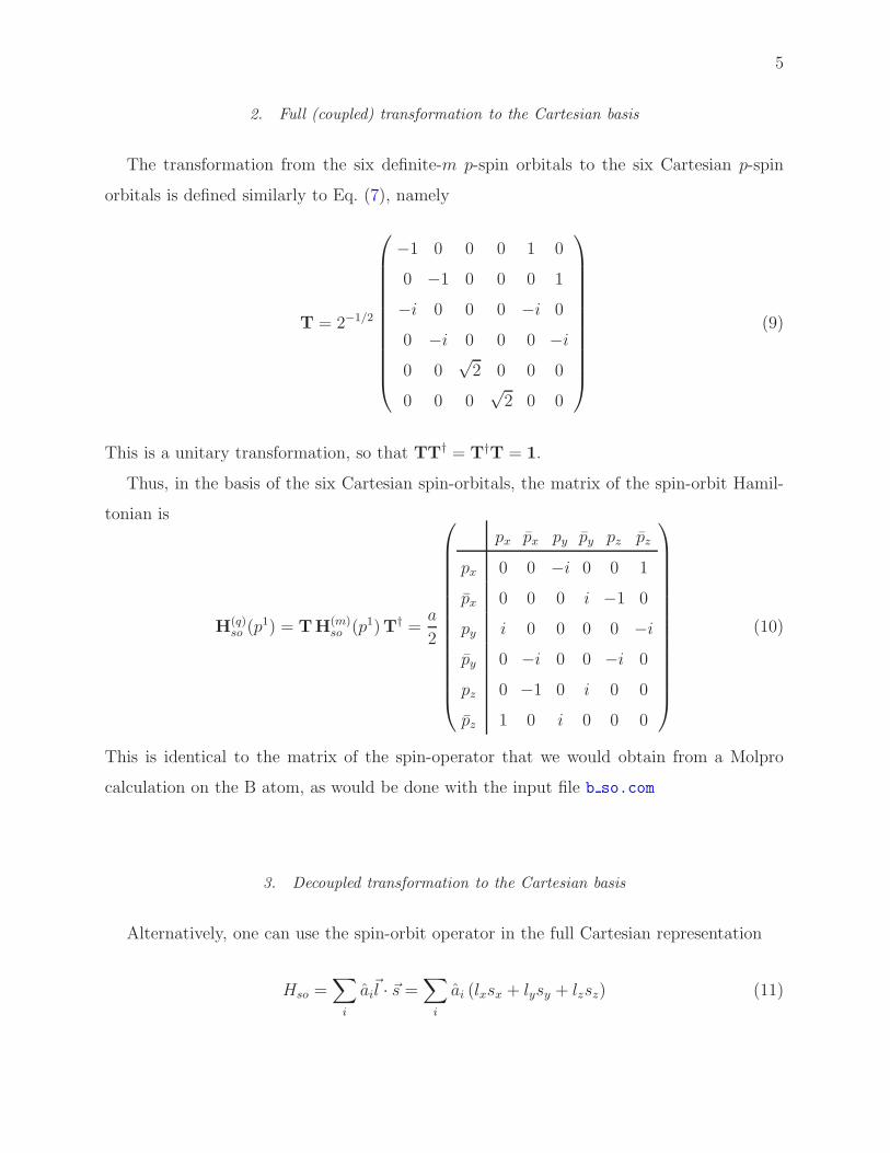
2. Full (coupled) transformation to the Cartesian basis

The transformation from the six definite-m p-spin orbitals to the six Cartesian p-spin

orbitals is defined similarly to Eq. (7), namely

T = 2−1/2

−1 0 0 0 1 0

0 −1 0 0 0 1

−i 0 0 0 −i 0

0 −i 0 0 0 −i

0 0√2 0 0 0

0 0 0√2 0 0

(9)

This is a unitary transformation, so that TT† = T

†T = 1.

Thus, in the basis of the six Cartesian spin-orbitals, the matrix of the spin-orbit Hamil-

tonian is

H(q)so (p

1) = TH(m)so (p1)T† =

a

2

px px py py pz pz

px 0 0 −i 0 0 1

px 0 0 0 i −1 0

py i 0 0 0 0 −i

py 0 −i 0 0 −i 0

pz 0 −1 0 i 0 0

pz 1 0 i 0 0 0

(10)

This is identical to the matrix of the spin-operator that we would obtain from a Molpro

calculation on the B atom, as would be done with the input file b so.com

3. Decoupled transformation to the Cartesian basis

Alternatively, one can use the spin-orbit operator in the full Cartesian representation

Hso =∑

i

ai~l · ~s =∑

i

ai (lxsx + lysy + lzsz) (11)

6

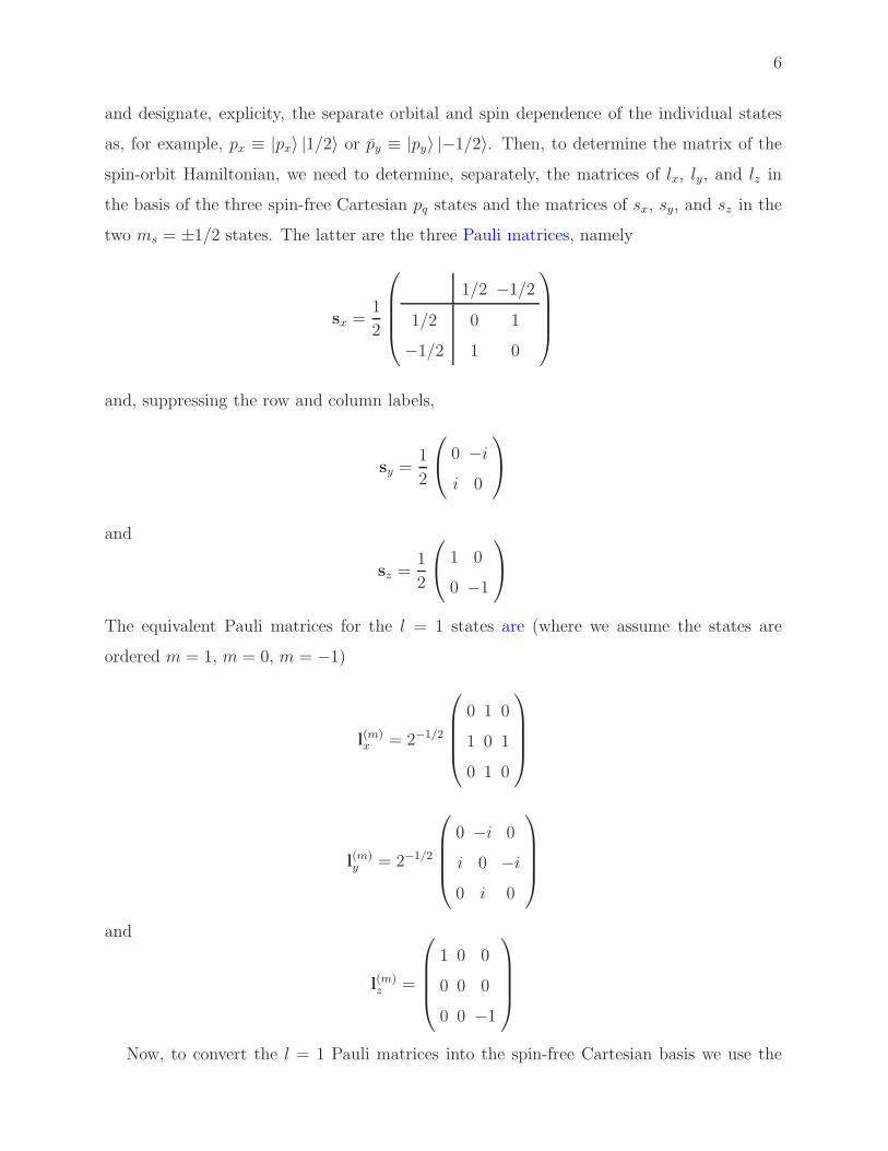
and designate, explicity, the separate orbital and spin dependence of the individual states

as, for example, px ≡ |px〉 |1/2〉 or py ≡ |py〉 |−1/2〉. Then, to determine the matrix of the

spin-orbit Hamiltonian, we need to determine, separately, the matrices of lx, ly, and lz in

the basis of the three spin-free Cartesian pq states and the matrices of sx, sy, and sz in the

two ms = ±1/2 states. The latter are the three Pauli matrices, namely

sx =1

2

1/2 −1/2

1/2 0 1

−1/2 1 0

and, suppressing the row and column labels,

sy =1

2

0 −i

i 0

and

sz =1

2

1 0

0 −1

The equivalent Pauli matrices for the l = 1 states are (where we assume the states are

ordered m = 1, m = 0, m = −1)

l(m)x = 2−1/2

0 1 0

1 0 1

0 1 0

l(m)y = 2−1/2

0 −i 0

i 0 −i

0 i 0

and

l(m)z =

1 0 0

0 0 0

0 0 −1

Now, to convert the l = 1 Pauli matrices into the spin-free Cartesian basis we use the

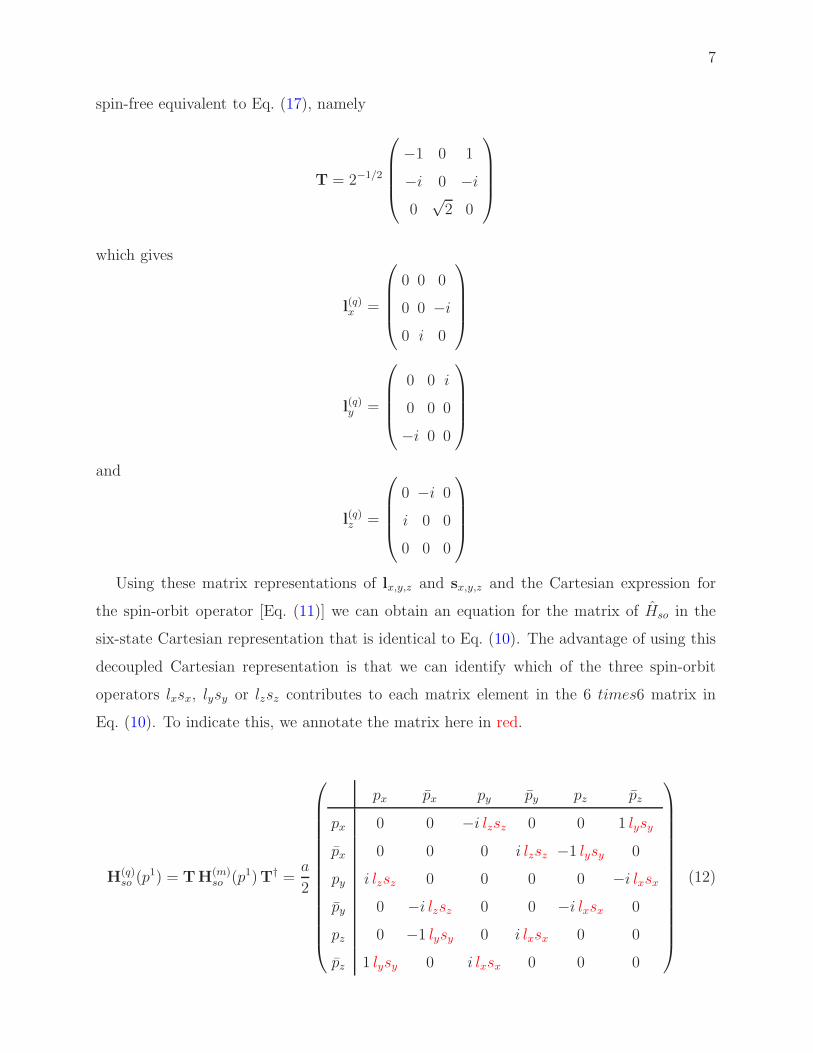
7

spin-free equivalent to Eq. (17), namely

T = 2−1/2

−1 0 1

−i 0 −i

0√2 0

which gives

l(q)x =

0 0 0

0 0 −i

0 i 0

l(q)y =

0 0 i

0 0 0

−i 0 0

and

l(q)z =

0 −i 0

i 0 0

0 0 0

Using these matrix representations of lx,y,z and sx,y,z and the Cartesian expression for

the spin-orbit operator [Eq. (11)] we can obtain an equation for the matrix of Hso in the

six-state Cartesian representation that is identical to Eq. (10). The advantage of using this

decoupled Cartesian representation is that we can identify which of the three spin-orbit

operators lxsx, lysy or lzsz contributes to each matrix element in the 6 times6 matrix in

Eq. (10). To indicate this, we annotate the matrix here in red.

H(q)so (p

1) = TH(m)so (p1)T† =

a

2

px px py py pz pz

px 0 0 −i lzsz 0 0 1 lysy

px 0 0 0 i lzsz −1 lysy 0

py i lzsz 0 0 0 0 −i lxsx

py 0 −i lzsz 0 0 −i lxsx 0

pz 0 −1 lysy 0 i lxsx 0 0

pz 1 lysy 0 i lxsx 0 0 0

(12)

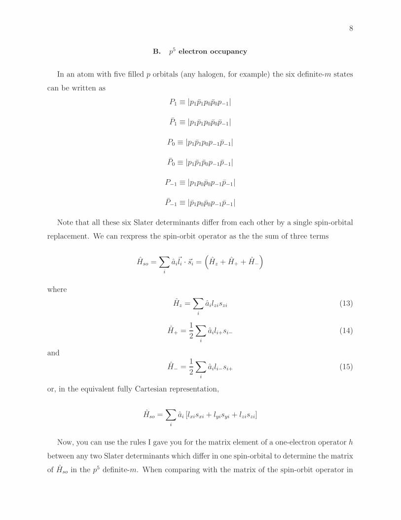
8

B. p5 electron occupancy

In an atom with five filled p orbitals (any halogen, for example) the six definite-m states

can be written as

P1 ≡ |p1p1p0p0p−1|

P1 ≡ |p1p1p0p0p−1|

P0 ≡ |p1p1p0p−1p−1|

P0 ≡ |p1p1p0p−1p−1|

P−1 ≡ |p1p0p0p−1p−1|

P−1 ≡ |p1p0p0p−1p−1|

Note that all these six Slater determinants differ from each other by a single spin-orbital

replacement. We can rexpress the spin-orbit operator as the the sum of three terms

Hso =∑

i

ai~li · ~si =(

Hz + H+ + H−

)

where

Hz =∑

i

ailziszi (13)

H+ =1

2

∑

i

aili+si− (14)

and

H− =1

2

∑

i

aili−si+ (15)

or, in the equivalent fully Cartesian representation,

Hso =∑

i

ai [lxisxi + lyisyi + lziszi]

Now, you can use the rules I gave you for the matrix element of a one-electron operator h

between any two Slater determinants which differ in one spin-orbital to determine the matrix

of Hso in the p5 definite-m. When comparing with the matrix of the spin-orbit operator in

9

the definite-m basis for a p1 electron occupancy [Eq. (1)], you find that the diagonal matrix

elements are changed in sign, since, for example

⟨

P1

∣

∣ Hso

∣

∣P1

⟩

= 〈|p1p1p0p0p−1|| Hz ||p1p1p0p0p−1|〉 =1

2− 1

2+ 0 + 0 +

1

2= +

1

2

The off-diagonal matrix elements are rearranged those in Eq. (1), since, for example

⟨

P1

∣

∣ Hso |P0〉 = 〈|p1p1p0p0p−1|| H+ ||p1p1p0p−1p−1|〉 = 〈p0| H+ |p−1〉

However, all the off-diagonal matrix elements in Eq. (1) are the same. Thus, in the definite-m

basis, the matrix of the spin-orbit operator for a state of p5 electron occupancy is

H(m)so (p5) =

a

2

P1 P1 P0 P0 P−1 P−1

P1 −1 0 0 0 0 0

P1 0 1√2 0 0 0

P0 0√2 0 0 0 0

P0 0 0 0 0√2 0

P−1 0 0 0√2 1 0

P−1 0 0 0 0 0 −1

(16)

Diagonalization gives eigenvalues of +a (two-fold degenerate) and −a/2 (four-fold degener-

ate), as we would anticipate for a p5 electron occupancy.

We write the 6 Cartesian states for a p5 electron occupancy as

Px ≡ |pxpypypzpz|

Px ≡ |pxpypypzpz|

Py ≡ |pxpxpypzpz|

Py ≡ |pxpxpypzpz|

Pz ≡ |pxpxpypypz|

Pz ≡ |pxpxpypypz|

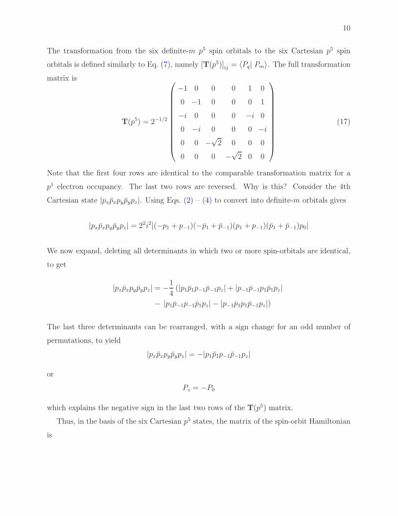
10

The transformation from the six definite-m p5 spin orbitals to the six Cartesian p5 spin

orbitals is defined similarly to Eq. (7), namely [T(p5)]ij = 〈Pq| Pm〉. The full transformation

matrix is

T(p5) = 2−1/2

−1 0 0 0 1 0

0 −1 0 0 0 1

−i 0 0 0 −i 0

0 −i 0 0 0 −i

0 0 −√2 0 0 0

0 0 0 −√2 0 0

(17)

Note that the first four rows are identical to the comparable transformation matrix for a

p1 electron occupancy. The last two rows are reversed. Why is this? Consider the 4th

Cartesian state |pxpxpypypz|. Using Eqs. (2) – (4) to convert into definite-m orbitals gives

|pxpxpypypz| = 22i2|(−p1 + p−1)(−p1 + p−1)(p1 + p−1)(p1 + p−1)p0|

We now expand, deleting all determinants in which two or more spin-orbitals are identical,

to get

|pxpxpypypz| = −1

4(|p1p1p−1p−1pz|+ |p−1p−1p1p1pz|

− |p1p−1p−1p1pz| − |p−1p1p1p−1pz|)

The last three determinants can be rearranged, with a sign change for an odd number of

permutations, to yield

|pxpxpypypz| = −|p1p1p−1p−1pz|

or

Pz = −P0

which explains the negative sign in the last two rows of the T(p5) matrix.

Thus, in the basis of the six Cartesian p5 states, the matrix of the spin-orbit Hamiltonian

is

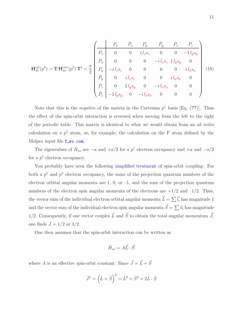
11

H(q)so (p

5) = TH(m)so (p5)T† =

a

2

Px Px Py Py Pz Pz

Px 0 0 i lzsz 0 0 −1 lysy

Px 0 0 0 −i lzsz 1 lysy 0

Py −i lzsz 0 0 0 0 i lxsx

Py 0 i lzsz 0 0 i lxsx 0

Pz 0 1 lysy 0 −i lxsx 0 0

Pz −1 lysy 0 −i lxsx 0 0 0

(18)

Note that this is the negative of the matrix in the Cartesian p1 basis [Eq. (??)]. Thus

the effect of the spin-orbit interaction is reversed when moving from the left to the right

of the periodic table. This matrix is identical to what we would obtain from an ab initio

calculation on a p5 atom, as, for example, the calculation on the F atom defined by the

Molpro input file f so.com.

The eigenvalues of Hso are −a and +a/2 for a p1 electron occupancy and +a and −a/2

for a p5 electron occupancy.

You probably have seen the following simplified treatment of spin-orbit coupling: For

both a p1 and p5 electron occupancy, the sums of the projection quantum numbers of the

electron orbital angular momenta are 1, 0, or –1, and the sum of the projection quantum

numbers of the electron spin angular momenta of the electrons are +1/2 and –1/2. Thus,

the vector sum of the individual electron orbital angular momenta ~L =∑~li has magnitude 1

and the vector sum of the individual electron spin angular momenta ~S =∑

~si has magnitude

1/2. Consequently, if one vector couples ~L and ~S to obtain the total angular momentum ~J ,

one finds J = 1/2 or 3/2.

One then assumes that the spin-orbit interaction can be written as

Hso = A~L · ~S

where A is an effective spin-orbit constant. Since ~J = ~L+ ~S

J2 =(

L+ S)2

= L2 + S2 + 2L · S

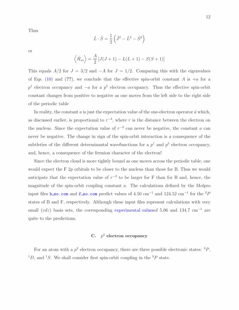
12

Thus

L · S =1

2

(

J2 − L2 − S2)

or⟨

Hso

⟩

=A

2[J(J + 1)− L(L+ 1)− S(S + 1)]

This equals A/2 for J = 3/2 and −A for J = 1/2. Comparing this with the eigenvalues

of Eqs. (10) and (??), we conclude that the effective spin-orbit constant A is +a for a

p1 electron occupancy and −a for a p5 electron occupancy. Thus the effective spin-orbit

constant changes from positive to negative as one moves from the left side to the right side

of the periodic table

In reality, the constant a is just the expectation value of the one-electron operator a which,

as discussed earlier, is proportional to r−3, where r is the distance between the electron on

the nucleus. Since the expectation value of r−3 can never be negative, the constant a can

never be negative. The change in sign of the spin-orbit interaction is a consequence of the

subtleties of the different determinantal wavefunctions for a p1 and p5 electron occupancy,

and, hence, a consequence of the fermion character of the electron!

Since the electron cloud is more tightly bound as one moves across the periodic table, one

would expect the F 2p orbitals to be closer to the nucleus than those for B. Thus we would

anticipate that the expectation value of r−3 to be larger for F than for B and, hence, the

magnitude of the spin-orbit coupling constant a. The calculations defined by the Molpro

input files b so.com and f so.com predict values of 4.50 cm−1 and 124.52 cm−1 for the 2P

states of B and F, respectively. Although these input files represent calculations with very

small (vdz) basis sets, the corresponding experimental valuesof 5.06 and 134.7 cm−1 are

quite to the predictions.

C. p2 electron occupancy

For an atom with a p2 electron occupancy, there are three possible electronic states: 3P ,

1D, and 1S. We shall consider first spin-orbit coupling in the 3P state.

13

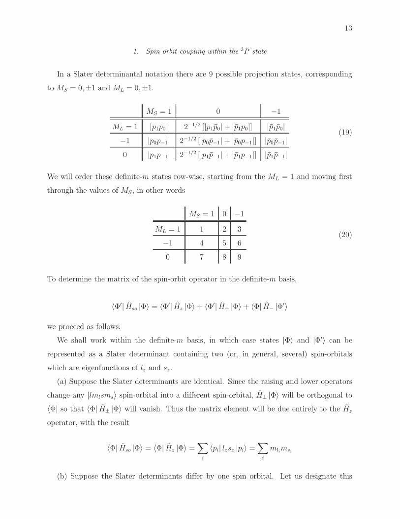
1. Spin-orbit coupling within the 3P state

In a Slater determinantal notation there are 9 possible projection states, corresponding

to MS = 0,±1 and ML = 0,±1.

MS = 1 0 −1

ML = 1 |p1p0| 2−1/2 [|p1p0|+ |p1p0|] |p1p0|−1 |p0p−1| 2−1/2 [|p0p−1|+ |p0p−1|] |p0p−1|0 |p1p−1| 2−1/2 [|p1p−1|+ |p1p−1|] |p1p−1|

(19)

We will order these definite-m states row-wise, starting from the ML = 1 and moving first

through the values of MS, in other words

MS = 1 0 −1

ML = 1 1 2 3

−1 4 5 6

0 7 8 9

(20)

To determine the matrix of the spin-orbit operator in the definite-m basis,

〈Φ′| Hso |Φ〉 = 〈Φ′| Hz |Φ〉 + 〈Φ′| H+ |Φ〉+ 〈Φ| H− |Φ′〉

we proceed as follows:

We shall work within the definite-m basis, in which case states |Φ〉 and |Φ′〉 can be

represented as a Slater determinant containing two (or, in general, several) spin-orbitals

which are eigenfunctions of lz and sz.

(a) Suppose the Slater determinants are identical. Since the raising and lower operators

change any |lmlsms〉 spin-orbital into a different spin-orbital, H± |Φ〉 will be orthogonal to

〈Φ| so that 〈Φ| H± |Φ〉 will vanish. Thus the matrix element will be due entirely to the Hz

operator, with the result

〈Φ| Hso |Φ〉 = 〈Φ| Hz |Φ〉 =∑

i

〈pi| lzsz |pi〉 =∑

i

mlimsi

(b) Suppose the Slater determinants differ by one spin orbital. Let us designate this

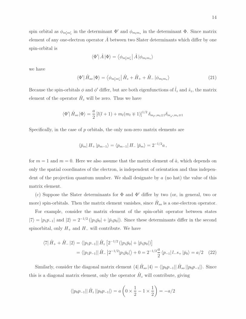
14

spin orbital as φm′

lm′

sin the determinant Φ′ and φmlms

in the determinant Φ. Since matrix

element of any one-electron operator A between two Slater determinants which differ by one

spin-orbital is

〈Φ′| A |Φ〉 =⟨

φm′

lm′

s

∣

∣ A |φmlms〉

we have

〈Φ′| Hso |Φ〉 =⟨

φm′

lm′

s

∣

∣ Hz + H+ + H− |φmlms〉 (21)

Because the spin-orbitals φ and φ′ differ, but are both eigenfunctions of lz and sz, the matrix

element of the operator Hz will be zero. Thus we have

〈Φ′| Hso |Φ〉 =a

2[l(l + 1) +ml(ml ∓ 1)]1/2 δm

l′,ml±1δm

s′,ms∓1

Specifically, in the case of p orbitals, the only non-zero matrix elements are

〈pm|H+ |pm−1〉 = 〈pm−1|H− |pm〉 = 2−1/2a ,

for m = 1 and m = 0. Here we also assume that the matrix element of a, which depends on

only the spatial coordinates of the electron, is independent of orientation and thus indepen-

dent of the projection quantum number. We shall designate by a (no hat) the value of this

matrix element.

(c) Suppose the Slater determinants for Φ and Φ′ differ by two (or, in general, two or

more) spin-orbitals. Then the matrix element vanishes, since Hso is a one-electron operator.

For example, consider the matrix element of the spin-orbit operator between states

|7〉 = |p1p−1| and |2〉 = 2−1/2 (|p1p0|+ |p1p0|). Since these determinants differ in the second

spinorbital, only H+ and H− will contribute. We have

〈7| H+ + H− |2〉 = 〈|p1p−1|| Hz

[

2−1/2 (|p1p0|+ |p1p0|)]

= 〈|p1p−1|| H−

∣

∣2−1/2|p1p0|⟩

+ 0 = 2−1/2a

2〈p−1| l−s+ |p0〉 = a/2 (22)

Similarly, consider the diagonal matrix element 〈4| Hso |4〉 = 〈|p0p−1|| Hso ||p0p−1|〉. Sincethis is a diagonal matrix element, only the operator Hz will contribute, giving

〈|p0p−1|| Hz ||p0p−1|〉 = a

(

0× 1

2− 1× 1

2

)

= −a/2

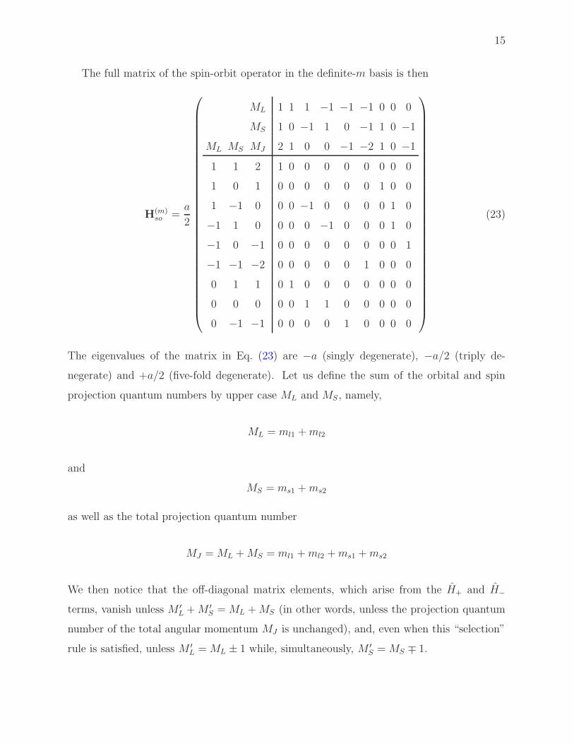
15

The full matrix of the spin-orbit operator in the definite-m basis is then

H(m)so =

a

2

ML 1 1 1 −1 −1 −1 0 0 0

MS 1 0 −1 1 0 −1 1 0 −1

ML MS MJ 2 1 0 0 −1 −2 1 0 −1

1 1 2 1 0 0 0 0 0 0 0 0

1 0 1 0 0 0 0 0 0 1 0 0

1 −1 0 0 0 −1 0 0 0 0 1 0

−1 1 0 0 0 0 −1 0 0 0 1 0

−1 0 −1 0 0 0 0 0 0 0 0 1

−1 −1 −2 0 0 0 0 0 1 0 0 0

0 1 1 0 1 0 0 0 0 0 0 0

0 0 0 0 0 1 1 0 0 0 0 0

0 −1 −1 0 0 0 0 1 0 0 0 0

(23)

The eigenvalues of the matrix in Eq. (23) are −a (singly degenerate), −a/2 (triply de-

negerate) and +a/2 (five-fold degenerate). Let us define the sum of the orbital and spin

projection quantum numbers by upper case ML and MS , namely,

ML = ml1 +ml2

and

MS = ms1 +ms2

as well as the total projection quantum number

MJ = ML +MS = ml1 +ml2 +ms1 +ms2

We then notice that the off-diagonal matrix elements, which arise from the H+ and H−

terms, vanish unless M ′L +M ′

S = ML +MS (in other words, unless the projection quantum

number of the total angular momentum MJ is unchanged), and, even when this “selection”

rule is satisfied, unless M ′L = ML ± 1 while, simultaneously, M ′

S = MS ∓ 1.

16

Alternatively, one can define 9 Cartesian states, which we define as

MS = 1 0 −1

xz |pxpz| 2−1/2 [|pxpz|+ |pxpz|] |pxpz|yz |pypz| 2−1/2 [|pypz|+ |pypz|] |pypz|xy |pxpy| 2−1/2 [|pxpy|+ |pxpy|] |pxpy|

(24)

We will order the Cartesian states similarly to Eq. (38), in other words

MS = 1 0 −1

xz 1 2 3

yz 4 5 6

xy 7 8 9

(25)

From Eqs. (2)–(4), it is easy to show that the transformation from the definite-m to the

Cartesian basis is

T = 2−1/2

−I −I 0

−iI iI 0

0 0 i√2I

(26)

where 0 is a 3 × 3 nul matrix and 1 is a 3 × 3 identity matrix. In deriving the expression

for this transformation matrix you have to be careful of phases. For example,

T14 = 〈|pxpz||p0p−1|〉 = 2−1/2〈(−|p1p0|+ |p−1p0|) |p0p−1|〉

= −2−1/2〈(−|p1p0|+ |p−1p0|) |p−1p0|〉 = −2−1/2 ,

and

T44 = 〈|pypz||p0p−1|〉 = 2−1/2〈(i|p1p0|+ i|p−1p0|)∗ |p0p−1|〉 = −2−1/2i〈(|p1p0|+ |p−1p0|) |p0p−1|〉

= +2−1/2i〈(|p1p0|+ |p−1p0|) |p−1p0|〉 = +2−1/2i ,

and

T77 = 〈|pxpy||p1p−1|〉 = 2−1 〈(−i|p1p−1|+ i|p−1p1|)∗ |p1p−1|〉 = +i

Similarly to Eq. (8) we can use the matrix of the spin-orbit operator in the definite-m

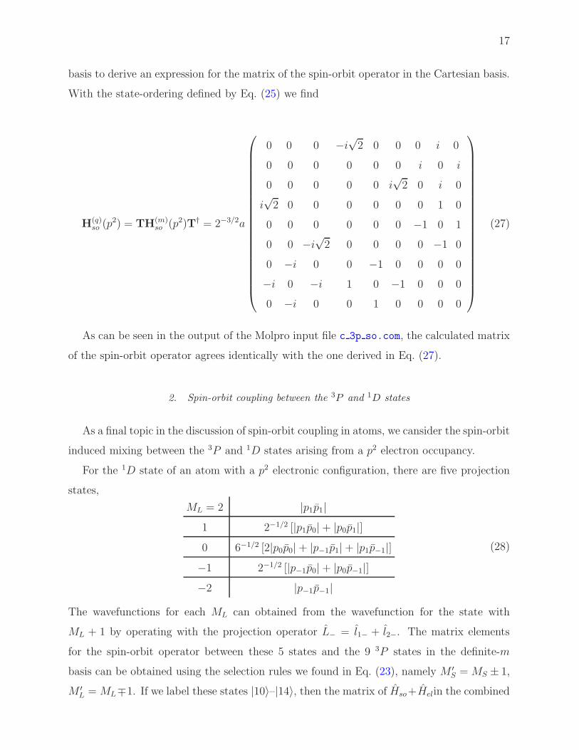
17

basis to derive an expression for the matrix of the spin-orbit operator in the Cartesian basis.

With the state-ordering defined by Eq. (25) we find

H(q)so (p

2) = TH(m)so (p2)T† = 2−3/2a

0 0 0 −i√2 0 0 0 i 0

0 0 0 0 0 0 i 0 i

0 0 0 0 0 i√2 0 i 0

i√2 0 0 0 0 0 0 1 0

0 0 0 0 0 0 −1 0 1

0 0 −i√2 0 0 0 0 −1 0

0 −i 0 0 −1 0 0 0 0

−i 0 −i 1 0 −1 0 0 0

0 −i 0 0 1 0 0 0 0

(27)

As can be seen in the output of the Molpro input file c 3p so.com, the calculated matrix

of the spin-orbit operator agrees identically with the one derived in Eq. (27).

2. Spin-orbit coupling between the 3P and 1D states

As a final topic in the discussion of spin-orbit coupling in atoms, we cansider the spin-orbit

induced mixing between the 3P and 1D states arising from a p2 electron occupancy.

For the 1D state of an atom with a p2 electronic configuration, there are five projection

states,

ML = 2 |p1p1|1 2−1/2 [|p1p0|+ |p0p1|]0 6−1/2 [2|p0p0|+ |p−1p1|+ |p1p−1|]−1 2−1/2 [|p−1p0|+ |p0p−1|]−2 |p−1p−1|

(28)

The wavefunctions for each ML can obtained from the wavefunction for the state with

ML + 1 by operating with the projection operator L− = l1− + l2−. The matrix elements

for the spin-orbit operator between these 5 states and the 9 3P states in the definite-m

basis can be obtained using the selection rules we found in Eq. (23), namely M ′S = MS ± 1,

M ′L = ML∓1. If we label these states |10〉–|14〉, then the matrix of Hso+Helin the combined

18

basis of the 9 definite-m 3P states plus the five definite-m 2D states is

H(m)el (3P/1D) +H

(m)so (3P/1D) = E(3P )1+

H(m)so (3P ) H

(m)13

[

H(m)13

]T

∆E

(29)

where H(m)so (3P ) is given by Eq. (23), 1 is a 14 × 14 unit matrix, ∆E is a 5 × 5 diagonal

matrix with elements equal to the difference between the energies of the 3P and 1D states,

namely

∆Eij = δij[

E(1D)− E(3P )]

,

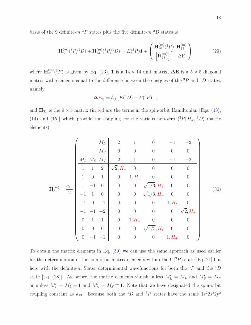
and H31 is the 9× 5 matrix (in red are the terms in the spin-orbit Hamiltonian [Eqs. (13),

(14) and (15)] which provide the coupling for the various non-zero 〈3P |Hso |1D〉 matrix

elements).

H(m)31 =

a132

ML 2 1 0 −1 −2

MS 0 0 0 0 0

ML MS MJ 2 1 0 −1 −2

1 1 2√2, H− 0 0 0 0

1 0 1 0 1, Hz 0 0 0

1 −1 0 0 0√

1/3, H+ 0 0

−1 1 0 0 0√

1/3, H− 0 0

−1 0 −1 0 0 0 1, Hz 0

−1 −1 −2 0 0 0 0√2, H+

0 1 1 0 1, H− 0 0 0

0 0 0 0 0√

4/3, Hz 0 0

0 −1 −1 0 0 0 1, H+ 0

(30)

To obtain the matrix elements in Eq. (30) we can use the same approach as used earlier

for the determination of the spin-orbit matrix elements within the C(3P ) state [Eq. 21] but

here with the definite-m Slater determinantal wavefunctions for both the 3P and the 1D

state [Eq. (28)]. As before, the matrix elements vanish unless M ′L = ML and M ′

S = MS

or unless M ′L = ML ± 1 and M ′

S = MS ∓ 1. Note that we have designated the spin-orbit

coupling constant as a13. Because both the 1D and 3P states have the same 1s22s22p2

19

electron occupancy, the magnitude of the spin-orbit constant should be very similar. As will

be seen below, in an actual calculation, the constants are the same at the level of the mean-

field approximation, [1] but slight differences occur when the full Breit-Pauli Hamiltonian is

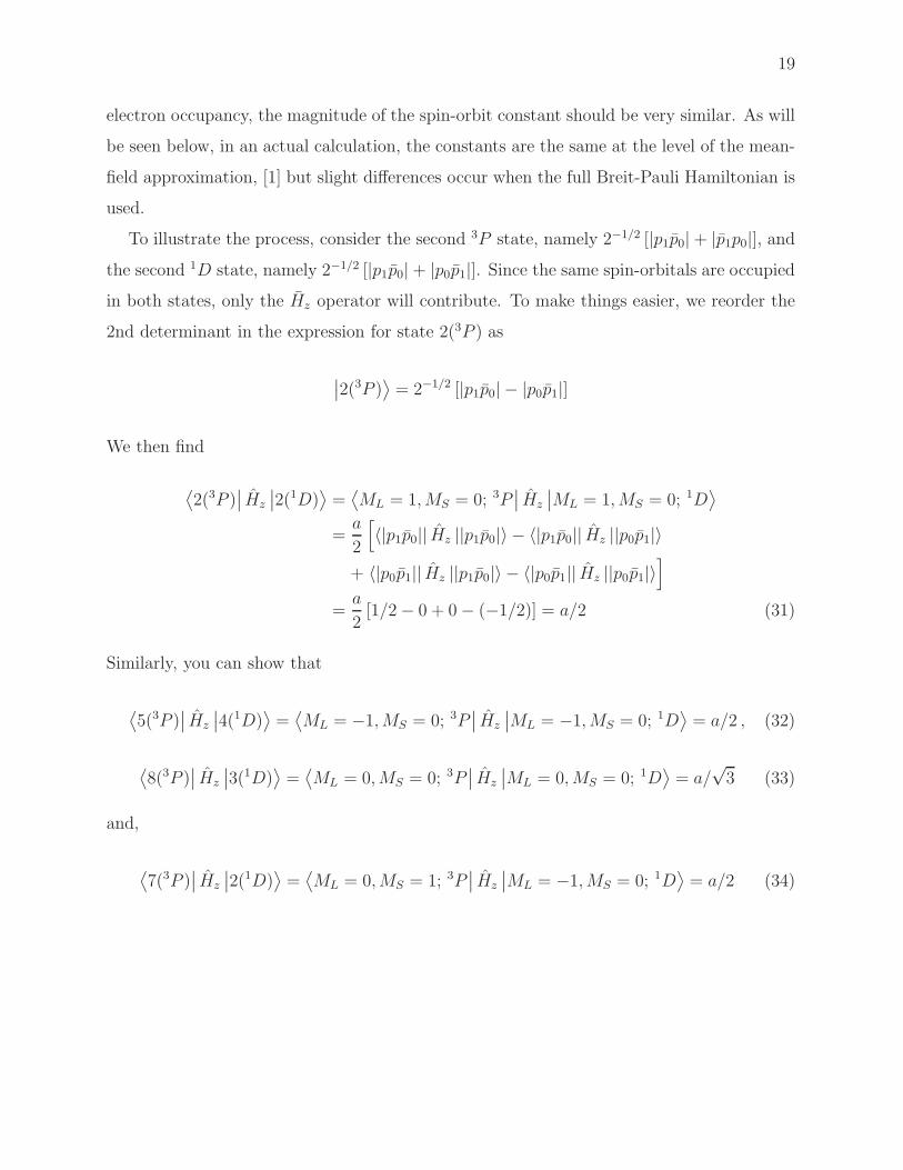
used.

To illustrate the process, consider the second 3P state, namely 2−1/2 [|p1p0|+ |p1p0|], andthe second 1D state, namely 2−1/2 [|p1p0|+ |p0p1|]. Since the same spin-orbitals are occupied

in both states, only the Hz operator will contribute. To make things easier, we reorder the

2nd determinant in the expression for state 2(3P ) as

∣

∣2(3P )⟩

= 2−1/2 [|p1p0| − |p0p1|]

We then find

⟨

2(3P )∣

∣ Hz

∣

∣2(1D)⟩

=⟨

ML = 1,MS = 0; 3P∣

∣ Hz

∣

∣ML = 1,MS = 0; 1D⟩

=a

2

[

〈|p1p0|| Hz ||p1p0|〉 − 〈|p1p0|| Hz ||p0p1|〉

+ 〈|p0p1|| Hz ||p1p0|〉 − 〈|p0p1|| Hz ||p0p1|〉]

=a

2[1/2− 0 + 0− (−1/2)] = a/2 (31)

Similarly, you can show that

⟨

5(3P )∣

∣ Hz

∣

∣4(1D)⟩

=⟨

ML = −1,MS = 0; 3P∣

∣ Hz

∣

∣ML = −1,MS = 0; 1D⟩

= a/2 , (32)

⟨

8(3P )∣

∣ Hz

∣

∣3(1D)⟩

=⟨

ML = 0,MS = 0; 3P∣

∣ Hz

∣

∣ML = 0,MS = 0; 1D⟩

= a/√3 (33)

and,

⟨

7(3P )∣

∣ Hz

∣

∣2(1D)⟩

=⟨

ML = 0,MS = 1; 3P∣

∣ Hz

∣

∣ML = −1,MS = 0; 1D⟩

= a/2 (34)

20

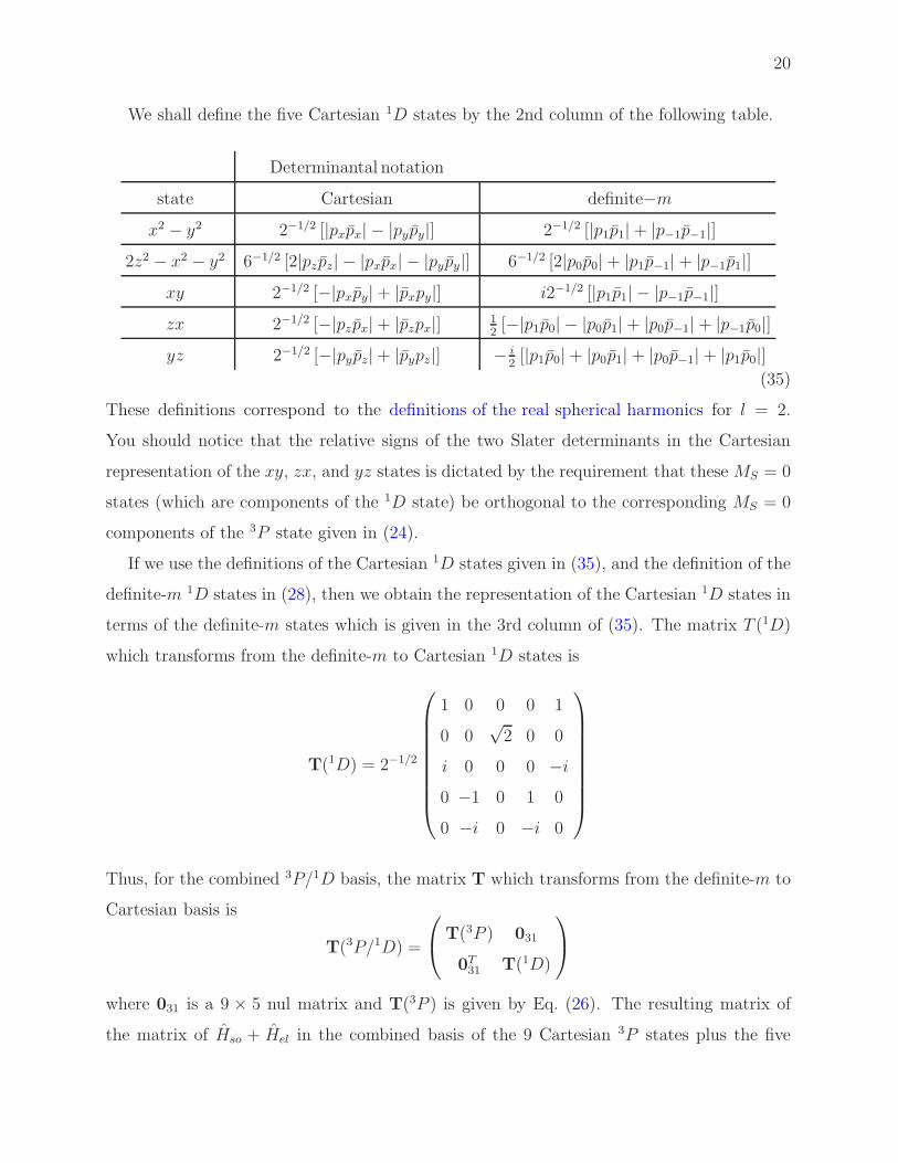
We shall define the five Cartesian 1D states by the 2nd column of the following table.

Determinantal notation

state Cartesian definite−m

x2 − y2 2−1/2 [|pxpx| − |pypy|] 2−1/2 [|p1p1|+ |p−1p−1|]2z2 − x2 − y2 6−1/2 [2|pzpz| − |pxpx| − |pypy|] 6−1/2 [2|p0p0|+ |p1p−1|+ |p−1p1|]

xy 2−1/2 [−|pxpy|+ |pxpy|] i2−1/2 [|p1p1| − |p−1p−1|]zx 2−1/2 [−|pzpx|+ |pzpx|] 1

2[−|p1p0| − |p0p1|+ |p0p−1|+ |p−1p0|]

yz 2−1/2 [−|pypz|+ |pypz|] − i2[|p1p0|+ |p0p1|+ |p0p−1|+ |p1p0|]

(35)

These definitions correspond to the definitions of the real spherical harmonics for l = 2.

You should notice that the relative signs of the two Slater determinants in the Cartesian

representation of the xy, zx, and yz states is dictated by the requirement that these MS = 0

states (which are components of the 1D state) be orthogonal to the corresponding MS = 0

components of the 3P state given in (24).

If we use the definitions of the Cartesian 1D states given in (35), and the definition of the

definite-m 1D states in (28), then we obtain the representation of the Cartesian 1D states in

terms of the definite-m states which is given in the 3rd column of (35). The matrix T (1D)

which transforms from the definite-m to Cartesian 1D states is

T(1D) = 2−1/2

1 0 0 0 1

0 0√2 0 0

i 0 0 0 −i

0 −1 0 1 0

0 −i 0 −i 0

Thus, for the combined 3P/1D basis, the matrix T which transforms from the definite-m to

Cartesian basis is

T(3P/1D) =

T(3P ) 031

0T31 T(1D)

where 031 is a 9 × 5 nul matrix and T(3P ) is given by Eq. (26). The resulting matrix of

the matrix of Hso + Hel in the combined basis of the 9 Cartesian 3P states plus the five

21

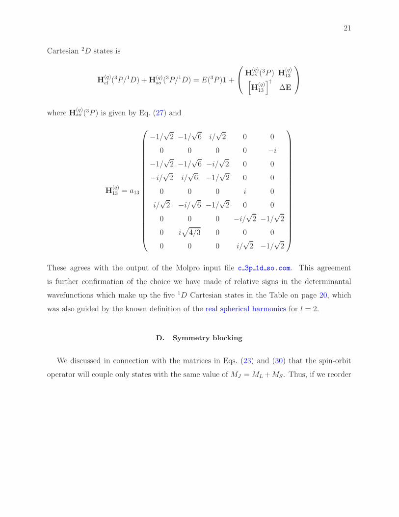
Cartesian 2D states is

H(q)el (

3P/1D) +H(q)so (

3P/1D) = E(3P )1+

H(q)so (3P ) H

(q)13

[

H(q)13

]†

∆E

where H(q)so (3P ) is given by Eq. (27) and

H(q)13 = a13

−1/√2 −1/

√6 i/

√2 0 0

0 0 0 0 −i

−1/√2 −1/

√6 −i/

√2 0 0

−i/√2 i/

√6 −1/

√2 0 0

0 0 0 i 0

i/√2 −i/

√6 −1/

√2 0 0

0 0 0 −i/√2 −1/

√2

0 i√

4/3 0 0 0

0 0 0 i/√2 −1/

√2

These agrees with the output of the Molpro input file c 3p 1d so.com. This agreement

is further confirmation of the choice we have made of relative signs in the determinantal

wavefunctions which make up the five 1D Cartesian states in the Table on page 20, which

was also guided by the known definition of the real spherical harmonics for l = 2.

D. Symmetry blocking

We discussed in connection with the matrices in Eqs. (23) and (30) that the spin-orbit

operator will couple only states with the same value of MJ = ML +MS. Thus, if we reorder

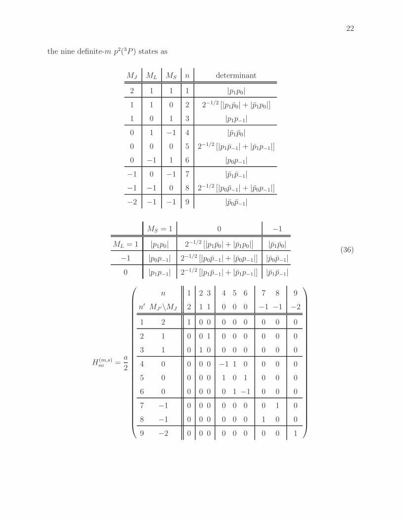
22

the nine definite-m p2(3P ) states as

MJ ML MS n determinant

2 1 1 1 |p1p0|1 1 0 2 2−1/2 [|p1p0|+ |p1p0|]1 0 1 3 |p1p−1|0 1 −1 4 |p1p0|0 0 0 5 2−1/2 [|p1p−1|+ |p1p−1|]0 −1 1 6 |p0p−1|−1 0 −1 7 |p1p−1|−1 −1 0 8 2−1/2 [|p0p−1|+ |p0p−1|]−2 −1 −1 9 |p0p−1|

MS = 1 0 −1

ML = 1 |p1p0| 2−1/2 [|p1p0|+ |p1p0|] |p1p0|−1 |p0p−1| 2−1/2 [|p0p−1|+ |p0p−1|] |p0p−1|0 |p1p−1| 2−1/2 [|p1p−1|+ |p1p−1|] |p1p−1|

(36)

H(m,s)so =

a

2

n 1 2 3 4 5 6 7 8 9

n′ MJ ′\MJ 2 1 1 0 0 0 −1 −1 −2

1 2 1 0 0 0 0 0 0 0 0

2 1 0 0 1 0 0 0 0 0 0

3 1 0 1 0 0 0 0 0 0 0

4 0 0 0 0 −1 1 0 0 0 0

5 0 0 0 0 1 0 1 0 0 0

6 0 0 0 0 0 1 −1 0 0 0

7 −1 0 0 0 0 0 0 0 1 0

8 −1 0 0 0 0 0 0 1 0 0

9 −2 0 0 0 0 0 0 0 0 1

23

E. p4 electron occupancy

For an atom with a p4 electron occupancy, as with an atom with a p2 electron occupancy,

there are three possible electronic states: 3P , 1D, and 1S. We shall consider here only

spin-orbit coupling in the 3P state.

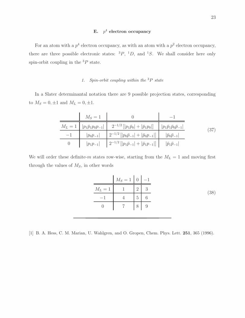
1. Spin-orbit coupling within the 3P state

In a Slater determinantal notation there are 9 possible projection states, corresponding

to MS = 0,±1 and ML = 0,±1.

MS = 1 0 −1

ML = 1 |p1p1p0p−1| 2−1/2 [|p1p0|+ |p1p0|] |p1p1p0p−1|−1 |p0p−1| 2−1/2 [|p0p−1|+ |p0p−1|] |p0p−1|0 |p1p−1| 2−1/2 [|p1p−1|+ |p1p−1|] |p1p−1|

(37)

We will order these definite-m states row-wise, starting from the ML = 1 and moving first

through the values of MS, in other words

MS = 1 0 −1

ML = 1 1 2 3

−1 4 5 6

0 7 8 9

(38)

[1] B. A. Hess, C. M. Marian, U. Wahlgren, and O. Gropen, Chem. Phys. Lett. 251, 365 (1996).