The vale-maintained tuning-fork as a precision time-standardrspa.royalsocietypublishing.org/content/royprsa/103/721/240.full.pdf · The Valve-maintained Tuning-fork as a Precision

240

The Valve-maintained Tuning-fork as a Precision Time-standard.B y D . D ye , B .S c.

(Communicated by Sir Joseph Petavel, F.R.S. Received January 13, 1923.)

(From the National Physical Laboratory.)

Introduction.

The system of driving a mechanical oscillator by means of a triode was first described by Eccles (1).

As applied to the maintenance of vibration of a tuning-fork, the method possesses very great advantages over any previously arranged electromechanical method. The complete absence of any attachments to the vibrator, together with the property of perfect self-starting, enables conditions of steadiness in operation to be realised which would not be otherwise possible. One such tuning-fork in use at the N.P.L. controls a multivibrator (2) and so forms the foundation of the radio-frequency standards of the laboratory.

In view of the great accuracy of measurement attainable, and of the importance of such a radio-frequency standard, it was thought desirable to make measurements on the controlling tuning-fork under various conditions, in order to ascertain what constancy and reliability might be expected under the conditions of use. The method used was one in which beats between two forks were measured by stop-watch, under conditions such that one fork was kept as invariable as possible, whilst the second fork had adjustments made in the various quantities which might be expected to cause variations in frequency.

Mounting of the Tuning-forks.

The forks will be designated A and B throughout the paper. Fork A had been used for two years for controlling the multivibrator. Fork B was made up specially to carry out this investigation and was almost identical with A, except that the air-gaps between the poles and the prongs of the fork were somewhat larger than on fork A.

The general arrangement of the mounting, also the electrical and physical quantities involved are given in fig. 1, below, which refers to fork B.

on June 23, 2018http://rspa.royalsocietypublishing.org/Downloaded from

http://rspa.royalsocietypublishing.org/

The principal dimensions are as follows:—Tuning-fork (Valentine and C arr)— Prong dimensions: breadth 9'0 mm.,

depth 13 9 mm., length 86 mm.Anode winding on bobbin Ci consists of about 9,000 turns of No. 4-/ d.s.c.

wire, having a d.c. resistance of 7,000 ohms.Grid winding on bobbin C3 consists of about 11,000 turns of No. 47 d.s.c.

wire, having a d.c. resistance of about 7000 ohms. Underneath the anode winding on Ci is an output winding of 2000 turns, No. 44 d.s.c. wire, having a resistance of 290 ohms.

The bobbins are fitted on to laminated iron-wire bundles, forming polar projections 1 cm. diameter of the polarising magnet, M. The air-gaps

Valve-maintainecl Tuning-fork as a Precision Time-standard, 241

Hole in ebonite cover for thermometer

F ig. 1.—Mounting of tuning-fork.

between the poles and the prongs of the tuning-fork are about 0*6 mm. Screws, S, serve to locate the magnet exactly with respect to the prongs of

* the fork. An ebonite cover-plate, E, clamps the magnet down on to the brass base and carries the terminals of the anode, grid, and output windings.

Fork A had a fixed condenser of 0004 mfd. capacity in parallel with the grid winding (Ci in fig. 2). On fork B variable condensers were used in parallel with both grid and anode windings.

The forks were encased in padded boxes and rested without constraint, loosely, on cotton-wool, so as not to cause any uncertain nodal points on the base, such as might occur if they rested on a partly solid support. Accurate thermometers, reading to 0-01° C., were mounted so that their bulbs came



between the prongs of the forks. The temperature conditions were steady in all the experiments.

The quantities investigated were:—(a) Temperature coefficient.

( b) Effect of variation of filament current and anode voltage.(c) Effect of variation of grid and anode condensers.( d) Effect of variation of polarising magnetic field.(e )Effect of variation of energy taken from the output winding.

( / ) Effect of adding various circuits in series in the anode circuit as an alternative means of taking out power.

(g) Effect of adding a mass to various parts of the mounting and of tiltingthe whole fork and mounting sideways and up and down.

(h) Absolute measurement of frequency.

Method of the Tests.

The arrangements for varying the quantities and observing the beats were as shown in fig. 2. Each tuning-fork and valve were fed by their own separate

242 D. Dye. The Valve-maintained

gj_ig 4=c jlj—2 m

F ig. 2.—Circuits for comparison of frequency of tuning-forks.

batteries, and the beats were observed on a Duddell vibration galvanometer, Y.G., tuned to the frequency of fork A. The mutual inductance couplings, Mi and M2, were small, and the reaction of one fork on the other through these mutuals was found to be entirely negligible. By adjustment of Mi or M2 the amplitudes of the vibration produced by each fork on the galvanometer were made exactly equal, so that when they were opposed during the beat the line came out quite sharply on the galvanometer spot. By this means the rate of the beats was observed with great accuracy. Even when



the beats were so slow that they were at the rate of one beat in 200 seconds, zero point could be located in time to within one or two seconds.

We will now turn to the particular quantities studied, in the order given previously in the paper.

(a) Temperature Coefficient.

This is one of the most serious causes of variation of frequency of a tuning fork. In the case of an ordinary simple tuning-fork with no attachments, the frequency coefficient is well established for the ordinary low- carbon steels. I t is chiefly due to the variation of the modulus of elasticity with temperature. For mild or cast-steel tuning-forks, the temperature coefficient of frequency is never very different from —1*15 x 10-4 per 1° C.

In the case of the valve-maintained tuning-fork, B, the coefficient was determined by placing the fork in its padded box in temperature-regulated vaults at various temperatures ; the fork was at least 48 hours in a sensibly constant temperature before observations were made. Fork A was kept under practically constant temperature conditions throughout the tests.

The results on both forks are given in Table I below.

Tuning-fork as a Precision Time-standard. 243

Table I.

Fork. Temperature range, 0 0.

Frequency coefficient per 1° O.

A 15-21 - 1 -l8x 10"4

B 15-21 - 1 -20x 10~4

these values are seen to be in close agreement with the accepted values for a free tuning-fork. The probable accuracy of these coefficients is ± 3 x 10-e.

% (b) Effect of Variation of Filament Current and Anode and(c) Effect of Variation of Grid and Anode Condensers.

Owing to the interdependence of (b) and (c) it was necessary to consider these together.

The following series of tests were therefore made:—(I) Anode Voltage Constant = 40 volts.

A family of curves was obtained giving change of frequency when anode current was varied by varying the filament brightness. Each curve corresponds to a particular value of grid capacity and a particular value of




anode capacity. The families of curves are thus really a series of interlacing families, and are distinguished by different kinds of lines.

The following cases were taken and are shown by the curves of fig. 3, in

- 1 0 o

g= o- 003a= o-ooo

j g = 0-003=Ha=o-ooi-----P -200

(g= 0-003 05 \a = 0 0 0 3

00 fg= 0-0025. J\&=0 005

------- la = o-oo3\ / g = 0-009

g=0-007 \a=o-ooo . a=o-oo3

t" \ f g= o '005 — la=ooo5

-5 0 0i 0-5 0-6Anode cu rren t — milliam pere

F ig. 3.—Variation of frequency with anode current varied by filament brightness.

which the various sets are distinguished by different kinds of lines as follows:—

Full-line Curves: Nos. 1, 2, 3 and4.—Added anode capacity = 0 mfd. Grid capacities of 0-003, 0*005, 0*007 and 0*009 mfd. respectively.

Dotted-line Curves: Nos. 5, 6 and 7. Added anode capacity = 0*003 mfd. Grid capacities of 0*003, 0*005 and 0*007 mfd.

Chain-line Curves: Nos. 8, 9, 10, 11, 12. Added anode capacity = 0*005 mfd. Grid capacities of 0*001, 0*0025, 0*0028, 0*003 and 0*005 mfd. respectively.



245Tuning-fork as a Precision Time-standard.

Two other eases (curves 13 and 14) were also taken with added anode capacity of 0-001 mfd. and added Grid capacity of 0 003 and 0-006 mfd.

These curves bring to light a number of interesting facts; some of these are explained in accordance with the theoretical treatment of the valve- maintained mechanical oscillator as given by Butterworth (3). There are, however, a number of factors variations of which can cause a change of frequency. These are not included in the mathematical assumptions, for example, the effective resistance of the anode-filament and the grid-filament paths of the valve itself, polarising field, output circuit, etc. These effects are so interdependent on one another that it is almost impossible to arrange the experiments so as to vary only one factor at a time. The changes in frequency due to anode and grid capacity variations are, however, so large that there is little doubt that they are mainly those developed by Butterworth and given in equations (19) and (20) in the paper previously referred to. Equation (19), giving variation of operating frequency when the electrical free frequency of the anode and grid circuits is varied, may be written

^ = 1+^ ? > wherea:= ^ - 1' «

This equation refers to the case where grid and anode windings are identical, and in which the capacities are varied so as to have always the same value on each winding.

The terms have the following meanings :—

*

o) = Frequency of steadily maintained vibration. ft>i = Free frequency of the fork.« = Equivalent mass of the fork = \ mass of one prong./3 = Damping coefficient in the fundamental equation of motion of the

fork.A = Force acting on the prong due to unit current in the grid or anode

winding./i = li/Lcoi where B and L are effective resistance and inductance of

grid or anode windings (windings assumed equal).2A2

Laft>i2 1 + /3R it is a term analogous to coupliug coefficient

between electrical circuits.Ihe various constants of the fork and associated circuits have been

approximately measured and are as follows :—Half mass of one prong = 45 grm. = a.

Log. dec. of fork as mounted = 0-0005, giving a value for of 45. free frequency of fork (nominal) = 1000 cycles per second.




A = 41 x 107 dynes per unit current (10 amperes) (obtained by observation of the change in the magnetic gap flux due to a small current sent through the anode coil).

The electrical constants were measured and were found to be :—Added capacity in parallel with the anode winding necessary to give

a frequency of resonance at 1000 cycles per second = 4*2 milli-mfd.For this test an inducing coil of 0-5 henry was used in series with the

anode coil, and an electrostatic voltmeter of about 100 yu,//, F. capacity was used as detector of resonance.

If we take the total resonating capacity to be 5 milli-mfd., including the voltmeter and leads and the self capacity of the anode coil, we get for the effective self-inductance of the anode winding the value L = 4’5 henries. The measured effective resistance of the anode winding at a frequency of 1000 cycles was found to be 27,000 ohms. (The d.c. resistance was about 7000 ohms.) These measurements were, of course, made with the fork held so that it could not vibrate.

From these two measurements the values of “ ya ” and were found to be yu2 == 0-95 and < = 7 2 x lO"4.

For the grid coil the resonant capacity was found to be 2*6 milli-mfds., giving, on the same assumptions as above, the values of 6‘9 henries for effective self-inductance of the grid winding.

The value of yu. assumed by Butterworth in calculating the curves showing- variation of frequency and ease of maintenance was y a = 0-02, nearly fiftytimes smaller than the experimental value found for this fork. The effect on the curves is to elongate the abscissa scale very greatly. For small values of “ x ” the formula for ratio of frequencies reduces to the very simple one

o)2/ ft>i2 = 1 + /j?. (2)

The formula so developed refers to the restricted case where the two electrical circuits are identical, i.e.the capacities across the (assumed equal) grid and anode winding sare always equal. The experiments were not carried out in a manner to suit these theoretical assumptions, and so cannot be directly compared with the theoretically calculated values of frequency change.

It will be seen from the curves (fig. 3), that the effects of capacity on grid or anode separately are very similar and in the same direction. Increasing- capacity causes a diminution in frequency, which is of the same order for variation of either grid capacity or anode capacity.

Confining attention to the curves in the region where they are nearly horizontal, we can use equivalent values of grid capacities corresponding to a grid



winding inductance equal to that of the anode winding. If now we add both capacities together we can calculate experimental values of “ ” and &>2/on3 — 1.

cIn deducing the values of x = —1 the value of Cres. has been taken as

0-0095 mfd. These results are plotted in fig. 4.The curve o>3/&>i3—1 = a2xjfj?is also drawn using the independently


+ 200

(C.res.= 0-0095 mfd.)

+ 100

+0-05 +0-10 +0-15 +0-20 +0-25-0-25 -0-20 -0-15 -0-10

------- 1-------- 1------------ 2001-------- 1----------1---------1------Fig. 4.—Effect on frequency of capacities across the windings.

determined values of a2 and fi2. The values of &>i3 read off from the curves are those corresponding to an anode current of 0-5 milliampere. J he irregularity of the experimental curve is not due to errors of observation, but indicates that it is not correct to add together the capacities in

♦the two circuits in the manner described above, or that it is incorrect to assume the same anode current for all the various cases. The rough agreement is, however, all that is intended to be shown.

Turning to these curves it will be seen that a remarkable compensating effect occurs in regard to frequency variation for curve (3). For an anode current variation from 0'25 to 0'6 milliamperes the maximum change in frequency is of the order of one part in a million only. Such an exactness of compensation is probably accidental, since, as will be seen later, changing the valve disturbs this compensation when changes of only a few parts in a million are in




question. This condition of compensation is of great value, and indicates that so long as the magnetic, mechanical, and electrical constants of the fork are invariable, then values of the latter can be chosen so that considerable variations of the voltages of the filament and anode batteries are of negligible consequence.

In further pursuance of the quantities governing this condition other combinations of grid and anode capacity were tried, and other similar cases were found as shown by the neighbouring curves. No case could be found, however, so good as that shown in curve Ho. 3.(II) Effect of Varying Anode Voltage.

An immense number of observations would have been involved in order to have investigated the foregoing capacity and anode current effects at a number of voltages; accordingly, only one capacity case was taken, viz., that case showing compensation, where C (grid) = O007 mfd., and C (anode) = 0 000 mfd. The results of these experiments are shown in fig. 5. In comparing these curves

-200

C onstan t filam en t b rig h tn ess

f ' S - 2 0 5

50 volts'u P- 210

70 v o lts

30 volts

-2 1 50-2 0-3 0-4 0-5 0 -6 0-7 0-8 1*0 1

Anode current — milliamuereF ig. 5.—Anode current: frequency curves for various anode voltages.

with those of fig. 3 it must be remembered that the scales are such that the curvature and slopes are magnified fifty-fold. I t should be mentioned here that a different valve was used in these experiments.

The voltage variation curves have been taken for one case of grid and anode capacities over the working range of anode current for each case of anode voltage. Variation of anode current was made by insertion of resistance in the filament battery circuit. A dotted curve is shown intersecting all



the other curves. This curve represents the change in frequency which occurs when nothing but the anode voltage is allowed to vary. There will, of course, be a whole series of such dotted curves for particular values of filament brightness, but only one such has been taken. These curves show that there is a best voltage from the point of view of variation of frequency with anode current, and also that at this voltage there is a best value of anode current from the point of view of variation of anode voltage. In the case of the particular valve used this point occurs with "70 volts on the anode and with an anode cuirent of about 1 milliampere. Under these conditions, a 10 per cent, change in either direction of anode current, or anode voltage, causes less than one pait in a million change in frequency.

Effect of Changing the Valve.—A variety of different valves were tried, all of the four-pin type, including a Mullard small filament current S.R. valve. The curves for these are given in fig. 6 for one anode voltage and the same


condenser case as above. I t will be seen that considerable variations can occur in frequency when one valve is changed for another. The points marked thus © show the frequency obtained for each valve, when any of them (except the S.R. valve) is simply plugged in on a fixed voltage of 4 volts.




Judged thus, it will be seen that there is little more than one part in 100,000 change in frequency when one valve is changed for another. The range of the curves represents a variation of 2 to 6 volts on the filament.

(d) Effect of Polarising Magnetic Field.This was known to be considerable and is probably caused by a change in

Young’s modulus or by a change in the mode of vibration. The method of experiment was very simple. An auxiliary permanent magnet was supported at varying distances from the magnet of the fork. By thus super-posing a magnetic field either helping or opposing the main field, a variation of 2 :1 could be made in the gap flux between the cores and prongs of the fork. The flux was measured by the help of a very thin search coil, which could be withdrawn from the narrow air-gap between the magnet cores and the prongs of the fork. The curve showing change of frequency plotted with gap-flux density is given in fig. 7. The curve shows that an increase in field strength

+200

^ + 100

1,500 1,600 1,700 1,800 1,900 2,000 2,100 2^ 00^ 2,^00 2,+00 2,500 2,600 2,700 Gap flux density ——sGauss

F ig. 7.—Effect of polarising field on frequency.

causes a lowering of frequency and also that this change is greater per unit change of field, with increasing field strength. The normal gap flux density was B = 2200. At this point a change of + 1 per cent, in gap flux causes a change of —6‘5 parts in a million in frequency. The change in flux density produced by an anode current of TO milliamperes was found by experiment to



be about fifty lines per sq. cm. With an anode current of 05 milliampere there should, therefore, be a change of fifteen parts in a million on reversal of the connection of both grid and anode windings. An experiment showed that the actual change in frequency was about eleven parts in a million which is as close agreement as could be expected in view of other effects probably accompanying a reversal of connections. From these results it will be seen that constancy of the polarising field to 1 per cent, is necessary, if constancy to a few parts in a million is desired in frequency. The method of mounting used by Eccles is probably better, but this method could not be used without constructing special magnets. I t was observed that weakening the field down to B = 1500 made very little difference to the amplitude of the fork.

(e) and (f). Effect of Taking Power from the System.The fork was originally intended to deliver a small amount of electrical

power from an output winding underneath the anode winding; as will be seen later it is preferable to take out power by means of circuits added in the anode circuit.

(e) Output Winding on same Gore as Anode Winding.—This case was very simple to deal with. Non-inductive resistances, from oc to 0, were connected across the output terminals and the effect on frequency observed by beats in the ordinary way. On some occasions the current was measured by a tuned Duddell vibration galvanometer in series, and on other occasions a low reading electrostatic voltmeter was used to measure the voltage across the external resistance.

The first case taken was that corresponding to invariability of frequency

Tuning-forlc as a Precision Time-standard. 251

with anode current. The conditions were :—

Anode volts .................................................... = 50.Anode current (varied somewhat with load) = 07 to 0*85 milliamp.Anode capacity........................... = O'OOOGrid capacity.................................................... = 0'007 yaF.

% The curves for this particular case are not given, but they were similar to those given in fig. 8. The change in frequency was about thirty parts in a million for an output of 100 microwatts. The smallness of output was disappointing in view of the relatively large change in frequency.

Tuning of the grid and anode windings was next resorted to in order to increase the power. The case chosen was that corresponding to approximate resonance in both grid and anode windings, viz., anode coil capacity = 0‘004 mfd., grid coil capacity 0'003 mfd. The results are shown in fig. 8. Curve A shows change of frequency with change of B, and curve B shows




output for various values of E. This case showed considerable improvement over the previous one, in that the maximum output was about seven times as

\T h d n ge of frequency N. curve

600 -30

B — Output curvedI 400 -20

Output winding' under anode winding Anode cap. = 0-004 Grid cap. =0-003200' -10

2,060500 ohms

500 ioyR(ohms)i,ooo 1,50010,000 ohms

F ig. 8. —Change of frequency with variation of electrical load on

great and at the same time the total change in frequency was no greater. Unfortunately the change of frequency is very rapid in the region where E is high. This is just what should be avoided if it is desired to couple the output winding to another amplifying system having an impedance which is high and which might be variable.

( / ) Experiments were next made using a mutual inductance with primary in the anode circuit and secondary connected to a variable resistance.

The first case tried consisted of a 100 millihenries mutual inductance, having primary self-inductance of about 250 millihenries and a secondary self-inductance of 100 millihenries. Its resistance was 40 ohms. Various resistances were again connected across the secondary winding and the changes in frequency observed together with the secondary current. The whole change in frequency was less than one part in a million for a variation of secondary resistance from infinity of 500 ohms. The output was, however, very small; the maximum being only about 100 microwatts. The open circuit secondary voltage was about 0*5. When the primary of the mutual was short-circuited a change of three parts in a million was produced.

A second case was taken using a larger mutual with lower resistance




primary and having a condenser across it. This very greatly augmented the power available, as shown by the curve B (fig. 9). Curve A again shows2,000 - 4 0 Output by mutual iuductan.ee having primary

in anode circuit, condenser across primary.M = 200 millih..

To anode' circuit of valve

| \-AMAAVWVVW _____ / 1 . I \ t .

Lx= 650millih. % L2= 60inillih.

B — Outp u t curve

Change: of frequency curve

3,000

F ig. 9.—Change of frequency with variation of electrical load on fork.

cnange of frequency for this case. I t will be seen that the total change of frequency possible over the whole range of secondary external resistance is no smaller than was the case with output winding on the driving core. The shape of the curve is, however, much better. When the grid-filament circuit of an amplifying valve was connected across the secondary of the mutual it caused a change in frequency of much less than one part in a million.

A number of curves connecting frequency with anode current were taken foi various values of secondary resistance in order to determine what effect the tuned circuit had on the isochronism with respect to anode current. Ihese are collected and labelled in fig. 10, from an inspection of these it will be seen that the effect of the large added impedance in the anode circuit is to steepen somewhat the curves connecting frequency and anode current.

Ihe whole change in frequency due to change of anode current from 0‘5 to 0 8 milliampere is only ten parts in a million for any value of secondary resistance from oo to 0. The relatively large change in frequency produced by the insertion of the large impedance of the tuned mutual circuit is well seen in these curves. If it is specially desired to amplify the power whenusing the fork as a source it will clearly be much more efficient to use a

vol. cm .—a. s



254

bigger mutual inductance. A mutual inductance of about 1 henry might be used giving a secondary voltage of about 12 volts. This applied to the

D. Dye. The Valve-maintained

1,000

0-6 [ . o-7Anode current—milliampere

Fig. 10.—Anode current: frequency curves for various electrical loads on fork.

grid filament circuit of an It valve using 200 volts anode potential would enable it to give practically all the power of which it was capable.

(g) Effect of Adding a Mass to Various Parts of the Mounting and of Tilting the whole ForJc Sideways and Up and Down.

A few simple experiments were tried of the effect of a mass placed in various positions as indicated on the diagram, fig. 11. The mass used was1 kgrm. , .,

The result of these experiments indicate that the position of the modal




surfaces can be appreciably changed by alteration of the effective mass of various parts. The effects are larger at the more flexible part of the base.

Position of Mass.Change in frequency,

parts in 10®.

- 8

+ 15

- 7

+ 3 2

F ig. 11.—Effect of mass on base of fork.

The effects of tilting the fork about are shown in the Table (fig. 12). The second and third columns show the position of the fork. The positions are also identified by the number in the first column.

Position “ elevation.” side end.

No.

c=f 1 !TQ 1

< =(c=^ g 2

! 0 3

Change in frequency.

Ox 10® -3x10®

- 7 x 10®

+ 10x10®

Fig. 12.—Effect of turning fork about.

It is interesting to note, in regard to positions 3 and 4, that a small change in frequency is to be expected on account of gravity. If we consider, as a rough approximation, that the prong behaves as a rigid beam of uniform section freely pivoted at its upper end, then, under the influence of gravity, it would have a frequency of oscillation given by 4 1 / 3as = 2\ J 2T w^ere = length of prong. For the case in question,

= cm,> giving ng = 2’1 complete vibrations per second. The proportional change of nof the fork due to a superimposed vibromotive force, which, acting alone, would give it a frequency ng, is given by

n — no — 4-n ~ * rt02'

lo r the case in question ■—— equals + l x l 0 ~ 6 according to whether the



256 L). Dye. The Valve-maintained

prongs point upwards or downwards. The effective length of the prong will be less than the true length because of flexure, but the gravity effect will be probably not more than doubled on this account.

The effects observed are therefore much larger than could be accounted for by gravity, but are in the same direction. The effect would be greater on forks of slower frequency, and would be proportional to (length)3'5 for forks of constant thickness of prong. The effect of turning a fork of 100 ~~ per second from an upright position through 180° might possibly be as great as 1 part in 10,000.

(h) Measurement of Absolute Frequency of the Fork.All the foregoing experiments have been carried out by observing

differences between two forks, one of which was kept under as constant conditions as possible. In order to determine the absolute frequency, it is, of course, necessary to compare the vibrations of the fork with time obtained by means of a standard clock giving seconds.

For this purpose a phonic wheel was constructed, and has proved most successful. The wheel is of aluminium, and carries a thin-toothed rim of steel. The mean diameter is about 11 cm., and there are twenty teeth and spaces each about 0'85 cm. circumferential length. The top of the teeth are

about 1*5 mm. above the bottom of the spaces. The proportions are therefore as in fig. 13.

A 50 :1 worm wheel driven by the phonic wheel carries a small contact pin, which thus closes the circuit through the chronograph once each 1000 alternations. This wheel and mounting has been very accuratelymade in one of the laboratory workshops, and the instant of closure of contact is certainly located to 1/1000 second. The wheel is provided with three magnets from Brown receivers. Two of these serve for running the wheel up to speed as a valve-driven motor on the principle described by Eccles (4). By means of a two-stage amplifier, sufficient energy can be obtained to run the wheel up to a speed of well over 3000 r.p.in., corresponding to a frequency of about 1100 per second. The grid magnet can be altered in its phase relation to the driving magnet. There is a third magnet mounted between the other two magnets. This one receives power from the fork by the help of a three-stage amplifier.

The synchronisation is very simply carried out. The wheel is run up to

F ig. 13.—Steel rim of phonic wheel.




spged controlling its own power. During this process the power from the tuning-fork is weakly applied to the tuning-fork driving magnet. A miiliammeter is included in the anode circuit of the valves feeding this magnet.

When the speed reaches that value corresponding nearly to synchronism with the fork, the beats are large on the miiliammeter needle. By careful adjustment of speed and steady increase of cunent in the tuning-fork magnet, the wheel is pulled into synchronism. The self-driving power is then smoothly reduced to zero, when the wheel then runs as a pure synchronous motor. In this way the tuning-fork records its own frequency directly on the chronograph without any attention and with extreme accuracy.

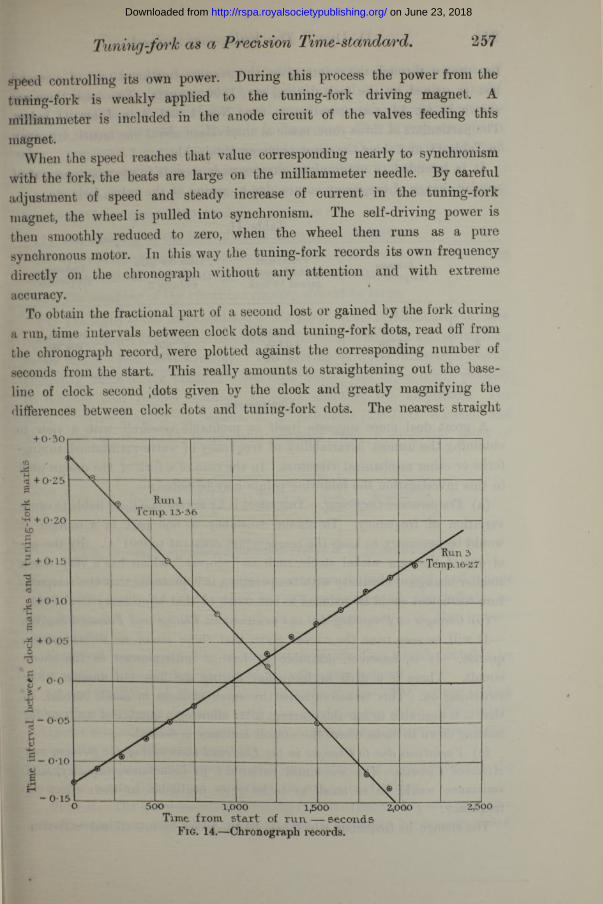
To obtain the fractional part of a second lost or gained by the fork during a run, time intervals between clock dots and tuning-fork dots, read off from the chronograph record, were plotted against the corresponding number of seconds from the start. This really amounts to straightening out the baseline of clock second .dots given by the clock and greatly magnifying the differences between clock dots and tuning-fork dots. The nearest straight




line drawn through the points gives the average fractional part of a second lost or gained by the fork during, say, 1500 seconds. Two such lines are shown in fig. 14, corresponding to runs Nos. 1 and 3 in Table II below. The particulars of three runs, made at intervals of about one month, are given in Table II, and show the great accuracy obtainable.

I t is intended to accumulate chronograph records to see what amount of secular change of frequency occurs, due to ageing of the valve, fork, etc.

Table II.

No. Averagetemperature.

Fractional part of second gained by fork.

Time for gain given in

Column 2.Deduced

frequency.

1°c.

13 -36 -0-39., 1 800 1000 -21s2 15 -23 + o -oo7 2 550 999 -997

999 -8703 16-27 + 0-297 2 250

Conclusions.A great deal more suggests itself as profitable research, with a view to

obtaining the utmost invariability of frequency of valve-maintained tuning- forks or other mechanical vibrators. In the case of a fork of the design used in this investigation the following points may be noted:—

(a) Temperature Coefficient.—This effect is by far the one most liable to cause variation of frequency. To obtain constancy to one part in a million, it would be necessary to keep the temperature constant to O'Ol0 C. By the use of one of the new nickel steels, such as “ elinvar,” which has a very much smaller change of elasticity with temperature, it is probable that the temperature coefficient could be reduced to one-tenth of that of ordinary steel forks.

(b) Changes in Frequency due to Variations in Voltage and Filament Sources.—It will be seen from the curves given that these are of no serious consequence. I t is, however, desirable to have a milliammeter in the anode circuit. There is a drift in frequency during the first ten minutes afterswitching on. This is accompanied by small changes in anode current, so that it is desirable to set this current after allowing a quarter of an hour for settling down in cases where the utmost accuracy is desired.

(c) Variations due to Changes in the Electrical Constants of the Driving and Attached Circuits.—The accidental variations in inductance, capacity, and resistance would be so small as to be quite negligible in their effect on frequency.

The change in frequency which can be produced by intentional variation




of grid-circuit or anode-circuit capacity forms a very convenient means of making changes of a few parts in a hundred thousand in frequency. By the use of a variable condenser of 0 001 mfd. range, a smooth reproducible variation of 5 parts in 100,000 can be made in frequency. This is very convenient when using such a source on certain bridges depending on frequency, and when measuring minute changes in capacity in oscillatory circuits.

In order that the attached electrical circuits may have the least effect on frequency if so required, the conditions then a re :—

(1) The damping of the fork must be as small as possible.(2) The dynamical energy associated with the motion of the fork should be

large compared with the electrical energy in the circuits.(3) The damping of the electrical circuits should be large.(d) The Effect of the Magnetisation of the Fork.—This is deleterious because

it causes increased damping of the fork and introduces stresses and controlling forces which react on frequency. The driving is quite satisfactory with polarising fields of the order of 1,000 e.g.s. un its; this value might possibly be reduced still further without seriously affecting the amplitude. The form of drive adopted by Messrs. E. A. Eckhardt (5), J. C. Karcher and M. Keiser, as in fig. 15, is probably superior from a magnetic point of

1j

To anode c ’ n —circu it — Li

rTo grid circuit

F ig. 15.—Self-maintained tuning-fork system of E. A. Eckhardt, etc.

view. In this system direct magnetic reaction between grid and anode circuits is used, but the author has no experience of the effects on frequency due to changes corresponding to those made in the present investigation.

Electrical capacity coupling to the prongs of the fork would probably be ♦very perfect if the air damping could be sufficiently reduced.

(e) and (f) Effect of Energy Taken from the System.—The energy is best taken from a circuit in series with the anode of the valve. For certain purposes this energy is sufficient, but for a great many others a simple one- or two-stage amplifier is necessary.

( 9)It is desirable to mount the fork very solidly and then to support thewhole on a soft diffused bed, or perhaps on soft pads of rubber.

General.—The valve-maintained tuning-fork is capable of operating with a steadiness of frequency which is greater than is necessary for most purposes



260 W. Stiles. The Indicator Method for the

The steadiness and invariability, which may be obtained by taking precautions, is very great. Such a time source, though secondary, opens up many possibilities in connection with investigations in which accurate short intervals of time are required. As an example of the use of such a time-standard it may be possible to observe variations in the hourly rate of standard clocks. This is of some importance in connection with absolute measurements of fundamental electrical units.

In conclusion, my best thanks are due to Sir Joseph Petavel for his kindly interest in the work, and to the Sub-Committee A of the Radio Research Board, in connection with whose researches some of the work was undertaken.

REFERENCES.

1. W. EL Eccles, ‘ Phys. Soc.Proc.,’ vol. 31, p. 269 (1919).2. H. Abraham and E. Bloch, ‘ C. R .,’ vol. 168, p. 1105 (1919).3. S. Butterworth, ‘ Phys. Soc. Proc.,’ vol. 33, p. 345 (1920).4. W. H . Eccles and F. W. Jordan, * Phys. Soc. Proc.,’ vol. 31, p. 151 (1919).5. E. A. Eckhardt, J . C. Karcher and M. Keiser, * Phys. Rev.,’ vol. 17, p. 535 (1921) ;

see also ‘ Journ. Franklin Inst.,’ vol. 174, p. 61 (1922).

The Indicator Method for the Determination of Coefficients of Diffusion in Gels, with Special Reference to the Diffusion of Chlorides.

By Walter Stiles, Sc.D., Professor of Botany in University College,Reading.

(Communicated by W. B. Hardy, Sec.R.S. Received February 18, 1923.)

Introduction.Since the original investigations of Thomas Graham on the diffusion of

dissolved substances in water a number of methods have been evolved and used for the determination of coefficients of diffusion of solutes in water. The essential feature of all these methods is the estimation of the quantity of dissolved substance after the lapse of a definite time in different layers of a cylinder of water through which the solute is diffusing, the calculation of the coefficient then being made on the assumption of Fick’s law, which defines the coefficient of diffusion as D in the equation

^ „ . 0C



Documents

The vale-maintained tuning-fork as a precision time-standardrspa.royalsocietypublishing.org/content/royprsa/103/721/240.full.pdf · The Valve-maintained Tuning-fork as a Precision