The tropical Madden-Julian oscillation and the global wind oscillation

Klaus Weickmann

NOAA/ESRL/Physical Sciences Division, Boulder, Colorado

Edward Berry

NOAA/National Weather Service, Dodge City, Kansas

Monthly Weather Review

Submitted

June 12, 2008

2

Abstract

The global wind oscillation (GWO) is a subseasonal phenomenon encompassing the

Madden-Julian Oscillation (MJO) and mid-latitude processes like meridional momentum

transports and mountain torques. A phase space is defined for the GWO following the

approach of Wheeler and Hendon (2004) for the MJO. In contrast to the oscillatory

behavior of the MJO, two red noise processes define the GWO. The red noise spectra

have variance at periods that bracket the 30-60 day band generally used to define the

MJO. The MJO and GWO correlation accounts for 25% of their variance and cross-

spectra show well-defined phase relations. However, considerable independent variance

still exists in the GWO. During MJO and GWO episodes, key events in the circulation

and tropical convection derived from composites can be used for monitoring and for

evaluating prediction model forecasts, especially for weeks 1-3. A case study during

April-May 2007 focuses on the GWO and two ~30 day duration orbits with extreme

anomalies in GWO phase space. The MJO phase space projections for the same time

were partially driven by mountain torques and meridional transports. The case reveals the

tropical-extratropical character of subseasonal events and its role in creating slowly

evolving planetary-scale circulation and tropical convection anomalies.

3

1. Introduction

Subseasonal, 10-90 day events in the atmosphere’s circulation evolve in the frequency

band that connects synoptic weather variations and interannual climate behavior. These

atmospheric fluctuations influence the statistics of extreme weather events and can

initiate rapid changes in the interannual climate. Such abrupt or extreme developments

are at the frontier of weather and climate prediction. Moreover, subseasonal variations

occur in a frequency band where both internal atmospheric dynamics and SST boundary

forcing are important. Understanding the time and space scales of this domain, and their

interaction with adjacent time bands, is a scientific challenge but is also important for

global climate modeling and extended range prediction.

The tropical Madden-Julian Oscillation (MJO; Madden and Julian, 1972) and the

extratropical teleconnection patterns (Wallace and Gutzler, 1981) are phenomena that

bridge weather and climate. They have inherent lifetimes between 10-90 days and are

linked with variations in the global or near-global circulation. Additional global

teleconnection patterns have been proposed by Branstator (2002) and Weickmann and

Berry (2007; hereafter WB). These global phenomena provide an index of the time-

evolving atmospheric circulation and the ongoing influence of coherent tropical

extratropical interactions. Synoptic experience shows that global AAM variations can be

linked to individual high impact weather events. This spatial and temporal mixture must

be properly represented in weather and climate models used for prediction and climate

simulation.

Atmospheric angular momentum (AAM) provides a convenient framework (Peixoto and

Oort, 1992) to track the global consequences of these subseasonal weather phenomena,

and is a starting point for monitoring their regional impacts. Nearly 30 years ago Langley

et al. (1981) documented the presence of ~50 day variations in length of day and global

AAM. Anderson and Rosen (1983) linked these variations to the MJO and analyzed a

coherent poleward and downward propagation of zonal mean zonal wind anomalies.

Global AAM anomalies peaked as the zonal mean zonal wind moved into the subtropics.

4

The link to the MJO was further explored by Madden (1987) who showed global AAM is

largest when MJO convection anomalies are weakening near the Dateline. Madden

(1987, 1988) proposed frictional torque anomalies over the Pacific Ocean basin to the

east of the convection anomalies were responsible for the exchange of angular

momentum between the atmosphere and the earth. Although the mountain torque

appeared to be small, subsequent investigations (Weickmann et al., 1992; Madden and

Speth, 1995; Hendon, 1995; Weickmann et al., 1997 hereafter WKS) proposed

approximately equal roles for the friction and mountain torque in forcing the global AAM

changes.

In contrast to the focus on the MJO, several studies (Ghil and Childress, 1987; Dickey,

Ghil and Marcus, 1991; Ghil and Robertson, 2002) argued for a separate ~40 day AAM

oscillation in the extratropical atmosphere forced primarily by the mountain torque and

its interaction with the asymmetric zonal circulation. Oscillatory forcing by the

extratropical mountain torque in the 20-30 day band was also proposed (e.g., Lott et al.,

2004; Lott et al., 2005). The idea of independent intraseasonal global AAM oscillations,

one forced by mountain torques in the extratropics and the other by convection in the

tropics was postulated and the former process studied by Marcus et al., (1994) and Jin

and Ghil (1990). Each oscillation would be capable of exciting the other so both tropical

convective and mountain torque signals would occur in individual cases (Madden and

Speth, 1995).

Weickmann, et al, 2000 (hereafter WRP) also argued for a separate mode of subseasonal

global AAM variation but rather than oscillatory they assumed its forcing and evolution

was stochastic. The underlying physics was linked to the atmosphere’s attempt to

maintain AAM balance in the presence of large or clustered mountain torque events. A

zonal mean analysis suggests impulsive momentum fluxes, especially across ~30-40N,

play a dual role of exciting the mountain torque and transporting the resulting momentum

from mountainous source region to frictional sink region via mid-latitude eddies. A

characteristic feature of this adjustment process is a quadrature relation in global time

series of the friction and mountain torque with the frictional torque leading. Coherent

5

variations of the circulation that accompany the process include the well-known PNA

teleconnection pattern and zonal index variations (Weickmann, 2003 hereafter W03).

The slowest time scale governing the global evolution of this mode is the ~6-day decay

time of the global frictional torque. A red noise spectrum (Wilks, 1995) with a 6-day

decay time would show broadband variance centered at 2Π x 6 days= ~40 days, and

thereby the frictional torque would force AAM at these periods. The MJO produces

variance in a similar frequency band and the interaction between it and the frictional red

noise process is viewed as a prototype for tropical-extratropical interaction. This

interaction process is poorly simulated in probably all general circulation models used for

weather and climate prediction or simulation - an assertion to be tested.

Using AAM as a framework, WB advocated a “top-down” approach to monitoring short

term climate and evaluating subseasonal predictions by GCMs. The approach includes

evaluation of zonal mean anomalies and the interaction of multiple time/space scale

physical processes within a dynamical weather-climate linkage framework. Global

indices provide the big picture on the atmosphere’s state and are used to infer the zonal

mean and then regional behavior of the circulation, including teleconnection patterns.

WB chose three indices to represent multiple subseasonal time scales. Daily indices of

the Madden-Julian Oscillation (MJO; Madden and Julian, 1972), the global frictional

torque and the global mountain torque were combined to construct four distinct phases of

a global synoptic dynamic model (GSDM) of the atmosphere.

In this study, a more objective definition of the GSDM is derived for monitoring and

prediction applications. This will involve combining the MJO, as defined by Wheeler and

Hendon (2004 hereafter WH), with the global wind oscillation (GWO) as defined by the

global relative atmospheric angular momentum (AAM) and its time tendency. Although

both “oscillations” produce signals in AAM, the MJO signal develops through tropical

convective forcing and the GWO signal is dominated by mid-latitude mountain forcing

and zonal wave energy dispersion. A case study is used to introduce the GWO and in a

companion paper the MJO and GWO are compared using a composite analysis.

6

In Section 3, we examine the relationship between the MJO and the GWO and contrast

their spectra and cross-spectra. We show that the MJO is embedded within the GWO but

that independent mid-latitude processes are important along with tropical convective

forcing. In Section 4 the phase-space plots for both oscillations are introduced and a

summary of the MJO and GWO features is presented. The phase plots are then used to

study for the period from April-May 2007. The results show tropical convective forcing,

while important, had weak projection on the MJO while the global wind oscillation

(GWO) projections were large and primarily forced by extreme mountain torque events.

The case study relationship between the global indices and the zonal mean flow

anomalies is also examined. Finally, a successful week 2 prediction of a western USA

trough in late May 2007 is related to a particular portion of the GWO phase space.

Summary and conclusions are in Section 5.

2. Data sets and calculations

The NCEP/NCAR reanalysis-1 (Kalnay et al., 1996) is the primary dataset used in the

study. The global integral of relative AAM and its time tendency is computed as

described by Weickmann and Sardeshmukh (1994) using daily averages of 4x daily

sigma (p/ps) level data. The global tendency is estimated from the global AAM time

series using a 4th order finite difference scheme. The anomalies are relative to a 1968-96

climatology and are standardized using 5-day average data from 1968-2006. The standard

deviations based on the entire record are shown in Table 1.

Zonal and vertical integrals are produced using 192x94 Gaussian grids. For AAM, a

zonal, vertical integrated anomaly of 1.0x1024 kg m2 s-1 corresponds to a vertical and

zonal mean zonal wind of 2.8 m/s at 30° and 8.4 m/s at 60°. For the AAM tendency, an

integrated anomaly of 1.0x1018 kg m2 s-2 corresponds to a vertical and zonal mean zonal

wind tendency of ~0.2 m s-1 day-1 at 30°.

7

3. The Madden Julian Oscillation versus the Global Wind Oscillation: cross-spectral and

spectral analysis

WH defined an empirical measure of the MJO from the first two EOFs of a multivariate

field consisting of a 15N-15S average of the 200 mb zonal wind, the 850 mb zonal wind

and OLR. They refer to the two EOF time series as RMM1 and RMM2. Using an

analogous approach, the GWO is defined by two dynamically related quantities: the

global relative AAM anomaly and its time tendency, which will be referred to as GWO1

and GWO2 respectively. Figure1 shows sample 120-day time series for the MJO and the

GWO during Jan-Apr 2006. Multiple time scales are readily apparent even in this short

record. The GWO has 10, 30 and 60 day trough to trough or peak to peak variations

while the MJO’s are more like 20, 30 and 40 days.

Not surprisingly the MJO and GWO are correlated since the MJO induces global torques

as it moves through the tropics, and GWO variations unrelated to the MJO can induce

tropical convection anomalies by impacting the large-scale tropical wind and sea level

pressure fields. The relation between the two is summarized in Table 1 where cross-

spectral results for 20-120 day and 30-60 day 1/frequency bands are shown. The indices

have the mean and mean seasonal cycle removed, thus the RMMs are not exactly as

defined by WH.

Several observations can be made from these results: 1) there is slightly more coherent

oscillatory behavior evident in the 30-60 day compared to the 20-120 day bands. The 30-

60 day COH2 are all around 0.3 confirming that a global AAM oscillation accompanies

the MJO as it moves east; 2) GWO1 (AAM) is correlated and nearly in-phase with

RMM2 while the correlation with RMM1 is somewhat weaker and almost in quadrature.

This relationship generally confirms Madden’s (1987) observation that global relative

anomaly AAM is large as MJO convection decays around the Dateline; 3) the phase

relations are nearly identical in the two bands but the amplitude (or variance explained) is

nearly doubled for GWO in the 20-120 day band; 4) the coherent variance is maintained

8

in the broader 20-120 day band, especially for GWO1 versus RMM2 suggesting shorter

and longer term tropical convective changes accompany changes in the GWO.

Fig. 2 shows frequency spectra of the two components of the MJO and GWO. The

comparison of the observed spectra to the red noise background emphasizes the primary

difference between the two phenomena. The MJO is an oscillation with a peak in both

RMM spectra at around 45 days. The GWO on the other hand is two red noise processes;

one with fast (2 days) and the other with slow (14 days) e-folding times that effectively

bracket the MJO’s 30-60 day variance band giving considerable overlap in their spectral

signature.

There is some structure in the GWO spectra worth commenting on. GWO1 has a nearly

significant peak at ~52 days tilted toward 30-60 days and this likely reflects MJO forcing.

The “peak”, however, is clearly atop a red noise background with a 14 day decay time

scale, a separate phenomenon from the MJO. The GWO2 spectrum forms a plateau of

variance from 5-40 days with a hint of separate maxima from 5-15 days and 25-40 days.

These are significant at the 95% level, at least with respect to the chosen red noise

background. The 5-15 day band reflects the global mountain torque produced by

synoptic wavetrains moving over the mountains (Iskenderian and Salstein, 1998, W03).

Such events induce small but discernible responses in global AAM as can be seen in Fig.

1a. The 25-40 day band is also dominated by the mountain torque (WRP), which has 2-3

times the variance of the frictional torque in this frequency range. This band is the

primary driver for both MJO and non-MJO portion of the GWO.

W03 found the MJO’s global AAM signal is forced primarily by the frictional torque and

to a lesser degree by the mountain torque. While a portion of the GWO variance is related

to the MJO, there are many subseasonal events where the mountain torque is much larger

than the frictional torque. This again suggests another process contributes to GWO

variability. From a global AAM perspective, the primary candidate is the atmospheric

response to large or clustered mountain torque events that drive AAM up and down. On

average, the frictional torque acts to return the AAM extracted by the mountains to the

9

solid earth, and its slow decay time scale (~6 days) helps set the typical “lifetime” of the

adjustment process. The ubiquitous quadrature relation between the mountain and

frictional torque in the subseasonal band further contributes to the GWO1 variance

concentration in the 30-90 day band. WRP discussed the global and zonal aspects of

global mountain torque events while W03 illustrated the horizontal patterns that

accompany them. The similar frequencies involved with the MJO and this mountain-

frictional torque adjustment process suggest the likelihood of mutual excitation and

interaction.

4. Phase Space Plots

The phase space plots introduced by WH are an efficient and objective way to monitor

the MJO. They are being applied widely for diagnostic research and by operational

centers to monitor their model’s prediction of the MJO

(http://www.cdc.noaa.gov/MJO/Forecasts). In this section, we introduce a similar phase

plot for the GWO and then in Section 5 apply both “oscillations” to subseasonal events

that occurred during northern spring 2007.

To start, the WH phase plot for the MJO is reproduced in Fig. 3 showing phases 1-8

defined as eight 45° segments in the 360° phase space. The text boxes inside the circle of

arrows highlight important events when compositing on the RMMs including the location

of tropical convection and changes in the large scale circulation. Outside the circle of

arrows, the components of the GWO when compositing on the RMMs are shown. The

orbits rotate counter-clockwise (CCW) during an eastward-propagating MJO but can

rotate clockwise for a variety of reasons including tropical waves (Roundy et al., 2008)

and SST anomalies. A by-now-familiar time-sequence of active tropical convective

regions and large scale circulation changes is depicted during a MJO orbit.

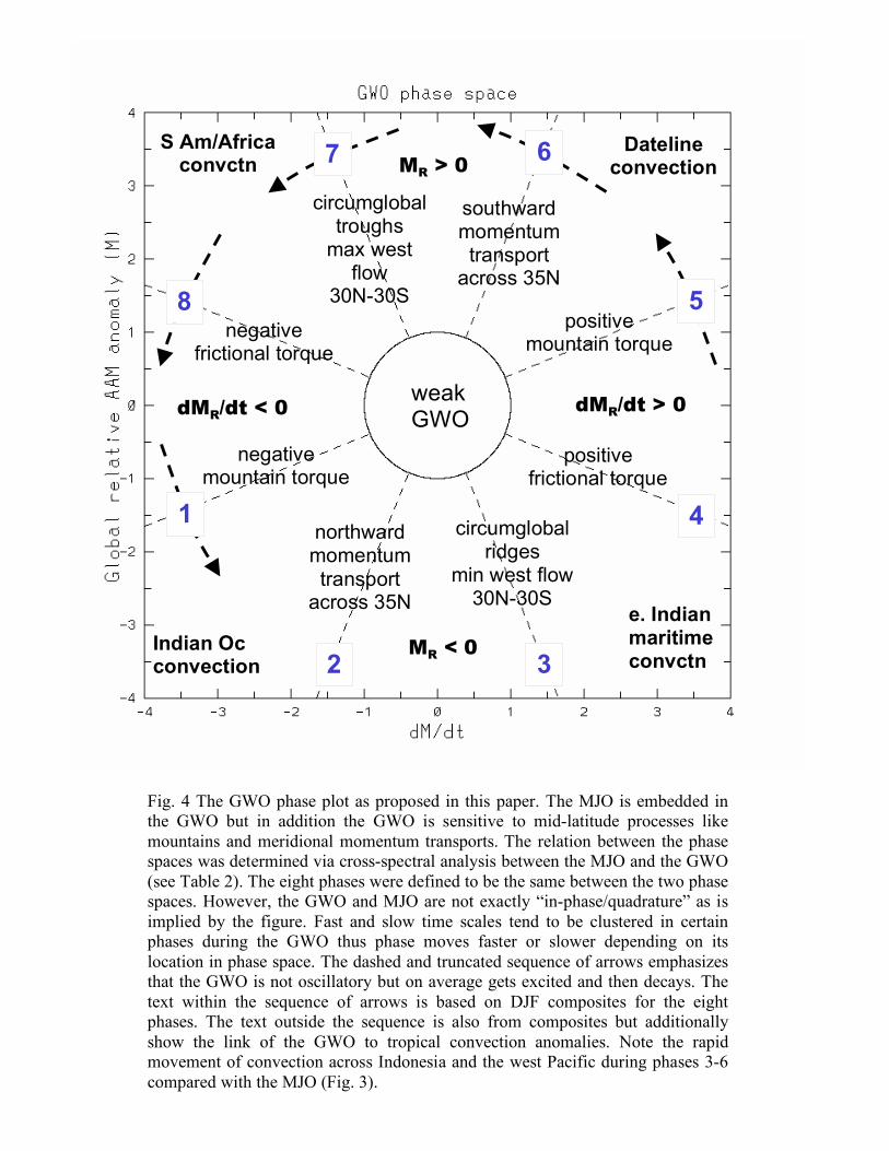
Figure 4 illustrates the phase space plotting format for the GWO. The phases match

those already defined by WH for the MJO. This will simplify real time monitoring and

comparing composites in the companion paper. The large, in-phase, coherence-squared

10

between GWO1 and RMM2 is used to define the relationship between the two phase

spaces. The dashed arrows show a schematic orbit in the GWO phase space, which can

only rotate CCW and need not be oscillatory. Westerly and easterly flows are exchanged

with the solid earth during an orbit.

Inside the arrows, important events in the circulation and related surface torques are again

shown while outside the arrows composites for tropical convection are shown. Along the

GWO phase space trajectory from 8 to 1, a negative global frictional torque is followed

by negative global mountain torque and together these processes give a strong negative

AAM tendency meaning westerly momentum is being removed from the atmosphere. A

regional-scale response is for the extended North Pacific Ocean jet to collapse, often

leading to a trough in the western USA (example discussed in Section 5). Monitoring

experience suggests that the global numerical models perform poorly in these situations,

and future work is planned to investigate this in models.

During phases 8 to 1 the tropical forcing is propagating eastward from the region of

South America into the Indian Ocean. As convection continues to shift into the Indian

Ocean, poleward AAM transports develop in the zonal mean at around 35N (and 35S).

This favors a northward shifted storm track and a circumglobal teleconnection

(Branstator 2002) pattern of anomalous midlatitude ridges by phase 3 (inter-hemispheric

symmetry). The latter base state is typical of La-Nina. The ability to anticipate certain

phenomena or processes provides an added dimension to a real time monitoring activity

devoted to extended range weather and climate forecasts.

5. Case Study: April-May 2007

a. Phase space plots

Fig. 5 is the MJO phase plot for the 59 days from 28 March to 25 May 2007 with a 5-day

running mean applied. In contrast to the standard plot (e.g., WH), interannual variations

are retained. This causes the center of the orbits to shift slightly (~0.5 sigma) toward the

11

“La Nina” phases 3-4. The MJO activity shows three coherent episodes where projections

of > one sigma or systematic eastward propagation occurred. These were interrupted by

two periods with nearly zero signals, 10-22 April and 8-15 May. The plot starts with a

MJO that developed over the Indian Ocean in mid-March 2007 (not shown) and is now in

phase 5. From phase 5, the MJO moves toward phase 1 before weakening around 10

April. The standard MJO phase plot (not shown) has > 1 sigma projections during this

time. Another weak event develops at the end of April 2007 at phase 2-3, moves east

briefly to phase 4-5 and weakens further ~6 May, but then re-intensifies to > 1 sigma at

phase 7 as it moves east through the “West. Hem. and Africa”.

The annotations on Fig. 5 depict four periods with extreme AAM tendency anomalies.

Together they produce two ~30 day GWO oscillations whose orbits in phase space will

be discussed shortly. The mountain torque contributes substantially to the extreme

tendencies. In Fig. 5, the two periods (10-22 April and 8-15 May) with near zero MJO

but extreme GWO2 projection are highlighted using thickened line segments. The

thickened segments occur just before MJO convection re-intensifies over the Indian

Ocean in late April and over the western Pacific in mid-May 2007. The connection is

highlighted using heavy black arrows. The composites to be presented in the companion

paper confirm these relationships between the GWO tendency and the subsequent

tropical convection anomalies.

Turning to the GWO, Fig. 6 shows its phase plot for the same period as the MJO in Fig.

5. The same dates have thickened line segments applied. Two prominent orbits are seen

during the 59-day period; one from 28 March to 25 April (29 days) and the other from 26

April to 26 May (31 days). The first is a single orbit while the second combines a fast and

slow orbit. On average the orbits are centered slightly away from zero toward phase 3-4

signifying a persistent negative global AAM anomaly, characteristic of a La Nina

circulation state. This is an important consideration when making a subseasonal forecast

or trying to understand the flow of waveguide wave energy.

12

The regularity of the GWO orbits contrasts with the more variable MJO projection seen

in Fig. 5. The relationship between the GWO and MJO projections discussed in that

figure is also evident in Fig. 6. Indian Ocean convection (IO) follows the extreme

negative tendency in mid-April and west Pacific Ocean (wPO) follows the extreme

positive tendency in early May. On the other hand, the other two extreme tendencies in

late May and early April are more integrated with the MJO convection anomalies so that

forcing and response is less clear-cut. For example, early in the first orbit, the eddies

responding to west Pacific tropical forcing and a positive mountain torque from the

Plateau of Tibet were easy to follow in daily weather maps. Atmospheric Rossby wave

dispersion, linked to both forcing mechanisms, clearly contributed to the zonal mean

southward momentum flux across 40N. This is consistent with the GWO feature seen at

phase 6 on Fig. 4 and will also be evident in the evolution of zonal AAM described in the

next section. It is just one example of a process that can be anticipated when the signals

in the GWO or the MJO are large and appear to be making a circuit or orbit.

More realistic subseasonal signals are clearly complex and it is not easy to disentangle

forcing-response-feedback. The main point is that subseasonal events evolve through the

mutual interaction between tropical convection and mid-latitude mountain-torque

dominated processes. For the zonal mean, the tropics and major mountainous regions are

linked via meridional momentum transports across 35N (35S). In the next section the

variations of the zonal mean circulation are related to the global MR, while the global

dMR/dt is shown to be dominated by mountain torques from three primary regions: the

Plateau of Tibet, the Rockies of North America and the Andes of South America.

b. Zonal-vertical integrals

Figure 7 presents the global and zonal-vertical integral of AAM anomalies corresponding

to Fig. 6. The bottom panel shows the two orbits in time series form while the top panel

shows the related zonal mean anomalies. The GWO phases and the location of positive

tropical convection anomalies have been marked on the bottom time series. Comparing

the top and bottom panels shows the orbits are produced by variations in the zonal mean

13

zonal flow, roughly in the region between 30N-30S. The long-term mean anomalies (>60

days) are negative in this region so Fig. 8a shows a pattern of easterly flow anomalies

interspersed with near zero anomalies; i.e., not westerly ones. The anomalies are shifting

poleward, a feature emphasized by highlighting the axis of positive AAM tendency in

Fig. 7a. The first orbit in early April has a fast, discontinuous northward shift in positive

zonal AAM tendency while the second in early May is slow and more coherent. These

shifts occur as AAM temporarily recovers from the low values seen in late March and

late April 2007.

Meridional momentum transports are the primary forcing for the poleward shifts and

while advection by tropical mass circulations may initiate the events, they are extended

poleward and in time by the mountain torque and favorable mid-latitude eddy structures.

Within the general Fig. 7a pattern of negative zonal mean zonal flows, there are time

periods and latitudes where westerly wind anomalies develop and persist. In the first orbit

this occurs near 35N while in the second it occurs more weakly near 20N and 15S. These

are related to a combination of the strong meridional momentum fluxes and large positive

mountain torques. The weak but positive global relative AAM anomalies seen in Fig. 7b

develop because of these zonal mean westerly wind anomalies. As shown below, these

zonal anomalies develop in latitude bands that contain the Asian, North American and

South American mountains. Although they are embedded in strong meridional flux of

zonal momentum, the mountains act as additional sources of momentum that have

downstream regional impacts and even can change the global or zonal mean zonal flow.

Figure 8 shows the zonal-vertical and global integral of the relative AAM tendency

corresponding to Fig. 7. The anomaly budget is dominated by the flux convergence of

AAM followed by the mountain torque, the frictional torque and the coriolis torque in

order of importance (WKS, W03). The purpose here is not to analyze the complete

budget but rather illustrate the timing of important physical processes during the two

GWO orbits. Recall that the orbits start after maximum easterly flow anomalies have

been established around 20N and 20S. The Fig. 8 top panel shows the negative tendencies

14

that create these anomalies and the positive tendencies that follow and weaken them after

the start of the orbits.

Despite the complicated structure of the tendency field, a careful comparison with Fig. 7

confirms a poleward movement of discrete negative and positive tendency events, and

these have been highlighted on the figure. They appear to emanate from north of the

equator in the Northern Hemisphere. The progression of negative and then positive

events is especially well defined during the second orbit. The flux convergence of AAM

is the primary driver for this behavior (WKS). Anomalous meridional mass circulations

forced by either tropical convection or eddy momentum fluxes likely drive the tropical-

subtropical tendencies while eddy momentum fluxes become the dominant driver at high

latitudes. The suggestive temporal connection in zonal mean flow anomalies for periods

of 1-3 months between the tropics and polar latitudes is not well understood dynamically

(Chang, 1998; Feldstein, 1998; Lorenz and Hartmann, 2001; Lee et al., 2007) but often

observed. On average, the MJO composite only gives propagation to 20N (20S) so it

provides no full explanation. In general the interplay between the momentum transports,

the mountain torque and tropical convective forcing is still poorly understood.

The flux convergence of AAM cannot produce a global AAM tendency but it can lead to

zonal wind anomalies that then produce zonal and global mountain torques. The two

large momentum transport events referred to previously are marked on Fig. 8 and

coincide with the two large global tendencies seen in the bottom panel. The meridional

transports are directed southward in early April and early-mid May. The colored curves

in the bottom panel confirm that mountain torques due to North American and Asian

topography make an important contribution to the first tendency and that South American

and Asian topography contribute to both the smaller tendency at the start of the second

orbit and the much larger tendency 10 days later.

A quantitative data analysis along with diagnostic modeling is required to understand the

complete progression of the AAM tendency curve seen in Fig. 8. But for forecasting

purposes, Fig. 3 and 4 illustrate an expected sequence of events that can be monitored

15

and anticipated, thereby helping to evaluate model predictions and a probable future

atmospheric state. In this case study, the events that typically accompany phases 8-1 were

used to forecast a western USA trough that developed ~20-23 May leading to severe local

storms on the Great Plains and significant temperature and precipitation anomalies across

the country. The initial forecast was based on the size of the positive tendency during ~10

May while in phase 4-5 and the fact that one orbit had already occurred. A well known

synoptic sequence accompanies phases 8-1: the Pacific jet stream strengthens, extends

east and then breaks down leaving a deep trough over the southwestern USA. The

acceleration of the zonal mean jet during the two orbits is seen by the large positive zonal

(global) AAM tendencies around 30N in Fig. 8a (Fig. 8b). The eddy forcing for the first

of these was described in the previous section. Of course the challenge is to determine

when/if the jet will break down, and this involves impacts from the synoptic as well as

the interannual state. These multi-time scale interactions cannot be ignored when

diagnosing subseasonal events.

6. Summary and Conclusions

The global wind oscillation (GWO) has been introduced as an additional aid to monitor

and help understand subseasonal variations of the global atmospheric circulation. It is

defined using global relative AAM and its tendency and when plotted in a phase space

diagram eight phases are defined. Frequency spectra were used to contrast the ~45 day

oscillations of the MJO with the multiple time scale, red noise behavior of the GWO.

A case study from April-May 2007 compares the time evolution of the GWO and the

MJO. The GWO was strong and coherent throughout the case compared to a transient

and weak projection for the MJO. The GWO variations were linked to zonal mean flow

anomalies in tropical regions between 30N-30S. During two well-defined GWO orbits,

anomalies of one sign in this latitude band are replaced with anomalies of opposite sign

while the original anomalies shift poleward Mountain torques embedded within strong

meridional momentum fluxes contributed additional momentum sources and sinks in

specific latitude bands and also had a major contribution to the global relative AAM

16

tendency. Zonal mean westerly wind anomalies were observed to emanate from the

latitude bands that contain major mountain ranges, especially Asia and South America.

The MJO can produce a signal in the GWO as shown by the moderate correlation

between them. However, it was argued that a separate mode of variation dominates the

GWO tied to the atmospheric circulation adjusting to large or clustered mountain torque

events. Both the MJO and the GWO produce zonal wind anomalies in the tropical band

and thus it is reasonable to suppose the oscillations can interact and excite one another.

These “oscillations” are being monitored in real time as the primary components of the

global synoptic dynamic model introduced by Weickmann and Berry (2007).

Understanding the dynamical processes explained by the GWO allows for a more

sophisticated evaluation of the numerical models as part of a complete forecast process.

A companion study uses the GWO to construct eight phase composites of zonal mean

and global teleconnection patterns. These are contrasted with the MJO’s composite

patterns. The composite differences suggest the GWO is dominated by zonal Rossby

wave dispersion while the MJO has prominent meridional dispersion of Rossby waves.

There is also a difference in the tropical convection centers of action. For the MJO the

Indian Ocean and west Pacific are at opposite phases but for the GWO it’s the Indian

Ocean and the Dateline region. The GWO-linked convection anomaly skips rapidly over

Indonesia and the west Pacific Ocean compared to the MJO convection anomaly.

Acknowledgements.

EKB expresses appreciation to Larry J. Ruthi, MIC, NOAA/NWS/WFO Dodge City,

Kansas, for his support of the project. Encouragement and support from Robin Webb

and Randy Dole are also appreciated.

References

17

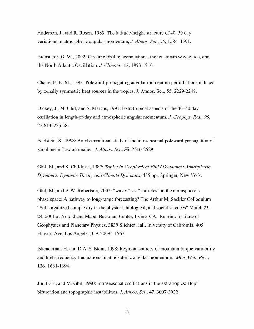
Anderson, J., and R. Rosen, 1983: The latitude-height structure of 40–50 day

variations in atmospheric angular momentum, J. Atmos. Sci., 40, 1584–1591.

Branstator, G. W., 2002: Circumglobal teleconnections, the jet stream waveguide, and

the North Atlantic Oscillation. J. Climate., 15, 1893-1910.

Chang, E. K. M., 1998: Poleward-propagating angular momentum perturbations induced

by zonally symmetric heat sources in the tropics. J. Atmos. Sci., 55, 2229-2248.

Dickey, J., M. Ghil, and S. Marcus, 1991: Extratropical aspects of the 40–50 day

oscillation in length-of-day and atmospheric angular momentum, J. Geophys. Res., 96,

22,643–22,658.

Feldstein, S., 1998: An observational study of the intraseasonal poleward propagation of

zonal mean flow anomalies. J. Atmos. Sci., 55, 2516-2529.

Ghil, M., and S. Childress, 1987: Topics in Geophysical Fluid Dynamics: Atmospheric

Dynamics, Dynamic Theory and Climate Dynamics, 485 pp., Springer, New York.

Ghil, M., and A.W. Robertson, 2002: “waves” vs. “particles” in the atmosphere’s

phase space: A pathway to long-range forecasting? The Arthur M. Sackler Colloquium

“Self-organized complexity in the physical, biological, and social sciences” March 23-

24, 2001 at Arnold and Mabel Beckman Center, Irvine, CA. Reprint: Institute of

Geophysics and Planetary Physics, 3839 Slichter Hall, Iniversity of California, 405

Hilgard Ave, Las Angeles, CA 90095-1567

Iskenderian, H. and D.A. Salstein, 1998: Regional sources of mountain torque variability

and high-frequency fluctuations in atmospheric angular momentum. Mon. Wea. Rev.,

126, 1681-1694.

Jin, F.-F., and M. Ghil, 1990: Intraseasonal oscillations in the extratropics: Hopf

bifurcation and topographic instabilities. J. Atmos. Sci., 47, 3007-3022.

18

Kalnay, E., and co-authors, 1996: The NCEP/NCAR 40-year reanalysis project: Bull.

Amer. Meteor. Soc., 77, 437-471.

Hendon, H. H., 1995, Length of day changes associated with the Madden-Julian

Oscillation. J. Atmos., Sci., 52, 2373-2383.

Langley, R. B., R. W. King, I. Shapiro, R. Rosen and D. Salstein, 1981: Atmospheric

angular momentum and the length of day: a common fluctuation with a period near 50

days. Nature, 294, 730-732.

Lee, S., S.-W. Son and K. Grise, 2007: A mechanism for the poleward propagation of

zonal mean flow anomalies. J. Atmos. Sci., 64, 849-868.

Lorenz, D. J. and D. L. Hartmann, 2001: Eddy-zonal flow feedback in the southern

hemisphere. J. Atmos. Sci., 58, 3312-3327.

Lott, F., A.W. Robertson and M. Ghil, 2004: Mountain torques and Northern-

Hemisphere low-frequency variability. Part I: Hemispheric aspects. J. Atmos. Sci., 61,

1259-1271.

Lott, F. and F. D’Andrea, 2005: Mass and wind axial angular-momentum responses to

mountain torques in the 1-25 day band: Links with the Arctic oscillation. Q, J. R.

Meteorol. Soc., 131, 1483-1500.

Madden, R. A., and P. R. Julian, 1972: Description of global-scale circulation cells in the

tropics with a 40–50 day period. J. Atmos. Sci., 29, 1109–1123.

Madden, R.A., 1987: Relationships between changes in the length of day and the 40- to

50- day oscillation in the tropics. J. Geophys. Res.,92, 8391-8399.

19

Madden, R.A., 1988: Large intraseasonal variations in wind stress over the tropical

Pacific. J. Geophys. Res., 93, D5, 5333-5340.

Madden, R.A. and P. Speth, 1995: Estimates of atmospheric angular momentum,

friction, and mountain torques during 1987-88. J. Atmos. Sci., 52, 3681-3694.

Marcus, S.L., M. Ghil and J.O. Dickey, 1994: The extratropical 40-day oscillation in the

UCLA general circulation model. Part 1: Atmospheric angular momentum. J. Atmos. Sci.,

51, 1431-1446.

Peixoto, J. P. and A. H. Oort, 1992: Physics of Climate (Chapter 11), Springer-Verlag

New York, Inc., 520 pp.

Roundy, P., C. Schreck and M. Janiga, 2008: Contributions of convectively coupled

equatorial waves and Kelvin Waves to the real-time multivariate MJO indices. Mon.

Wea. Rev., submitted.

Wallace, J.M. and D.S. Gutzler, 1981: Teleconnections in the geopotential height field

during Northern Hemisphere winter. Mon. Wea. Rev., 109, 784-812.

Weickmann, K. M., S.J.S. Khalsa and J. Eischeid, 1992: The atmospheric angular

momentum cycle during the tropical Madden-Julian Oscillation. Mon. Wea. Rev.,

120, 2252-2263.

Weickmann, K.M., 2003: Mountains, the global frictional torque, and the circulation over

the Pacific-North American Region. Mon. Wea. Rev., 131, 2608-2622.

Weickmann, K.M., W.A. Robinson, and C. Penland, 2000: Stochastic and oscillatory

forcing of global atmospheric angular momentum. J. Geophys. Res., 105, D12, 15543-

15557.

20

Weickmann, K.M. and P.D. Sardeshmukh, 1994: The atmospheric angular momentum

cycle associated with a Madden-Julian oscillation. J. Atmos. Sci., 51, 3194-3208.

Weickmann, K.M., G.N. Kiladis and P.D. Sardeshmukh, 1997: The dynamics of

intraseasonal atmospheric angular momentum oscillations. J. Atmos. Sci., 54, 1445-1461.

Weickmann, K.M., and E. Berry, 2007: A synoptic-dynamic model of subseasonal

atmospheric variability. Mon. Wea. Rev., 135, 449-474.

Wilks, D. S., 1995: Statistical methods in the atmospheric sciences. Volume 59,

International Geophysics Series, Academic Press, 467pp.

Wheeler, M. C., and H. H. Hendon, 2004: An all-season multivariate MJO index:

Development of an index for monitoring and prediction. Mon. Wea. Rev., 132, 1917-

1932.

21

Table 1: Standard deviations for the global wind oscillation (GWO)

In AAM units and global mean zonal wind

GWO1 (Relative AAM) GWO2 (Rel. AAM Tend.)

Daily data 1.2x1025 kgm2s-1

0.5 ms-1

1.9x1019 kgm2s-2

0.07 m s-1 day-1

Pentad data 1.2x1025 kgm2s-1

0.5 ms-1

1.4x1019 kgm2s-2

0.05 m s-1 day-1

Table 1. The annual mean global relative AAM is equivalent to a global mean zonal

momentum (ucosφ) of ~13 m/s. Pentad averaging does not remove much noise from the

relative AAM time series although it decreases standard deviation of the global AAM

tendency by 25%. This is consistent with their e-folding times.

22

Table 2. Cross spectrum analysis between the MJO and GWO

Entries: coherence-squared (correlation), phase in radians

Frequency band 20-120 day periods 30-60 day periods

“Oscillations” RMM1 (0.58) RMM2 (0.65) RMM1 (0.35) RMM2 (0.38)

GWO2 (0.4, 0.2) 0.2 (.45), 0.2 0.27 (.52), -1.3 0.27 (.52), 0.3 0.31 (.56), -1.4

GWO1 (0.28, 0.14) 0.21 (.46), 1.9 0.33 (.57), 0.2 0.28 (.53), 1.8 0.34 (.58), 0.2

Table 2. Cross-spectral analysis is shown between the MJO and the GWO for two

frequency bands using daily, standardized anomalies. The numbers following the indices

are the fractional variance contained in the frequency bands (e.g., (0.58) means 20-120

day band contains 58% of the variance). For the GWO in column1, the numbers in

parentheses refer to the variance fraction for 20-120 day and 30-60 day bands,

respectively.

23

Fig. 1 The daily anomaly time series of: a. GWO1 (global relative AAM, blue line) and GWO2 (global relative AAM tendency, red line) for Jan-April 2006, b. RMM1 (blue) and RMM2 (red) for the same time period. The panels are annotated with the duration of some selected “oscillations”.

RMM2 (wPac / Indian)

RMM1 (Maritime / WH)

Jan Feb Mar Apr

dMR/dt

MR

2006

30

10

60

30

30

30

40

50

40

20

GWO

MJO

a

b

24

partly MJO

RMM1 RMM2

GWO1

2π*14d 2π*2d 2π*14d 2π*2d

2π*14d

GWO2 2π*2d

τM

20-30d, MJO, etc.

MJO MJO

a b

c

d

Fig. 2 The frequency spectra for the components of the MJO (a, b) and the GWO (c, d). The blue line is the observed spectrum, the red line is a red noise background (obtained from the e-folding time of the time series, see text) and the black line is the 95% level of the red noise spectrum. The spectra are plotted with log frequency as the abscissa and with frequency multiplied by variance as the ordinate. This is a variance-conserving plot. In this type of presentation there is a “peak” in a red noise spectrum whose location is proportional to the decay or e-folding time of the time series, and 50% of the variance is contained on either side of this “peak”. The degrees of freedom (dof) for the 95% levels were estimated from the number of data points divided by the e-folding time of the time series. This gives: a) 7.2 dof/bin, b) 7.2, c) 5.4 and d) 38 dof/bin.

25

western Pacific

convection

meridional RWD PNA+

west hemisphere/ Africa convection

transition to twin subtropical anticyclones

W Pac cyclones

Indian Ocean

convection

meridional RWD PNA-

transition to twin subtropical cyclones w Pac anticyclones

Maritime continent convection

MR > 0

MR < 0 dMR/dt < 0

dMR/dt > 0

weak MJO

8

1

7 6

5

4

3 2

Fig. 3 The MJO phase plot as proposed by Wheeler and Hendon (2004). Two multivariate EOFs are used to define a 2-D phase space that is divided into 8 octants or segments, each covering 45°. The sequence of arrows depicts the rotation of the phase vector when an MJO is active and propagating eastward. For example, phase 2-8 would describe the development of convection over the Indian Ocean and its later demise over the western hemisphere. The text within and outside the sequence of arrows is based on DJF composites using the eight phases. The labels on the axes are standardized anomalies so the orbit shown by the sequence of arrows an amplitude of 3.5 sigma.

26

circumglobal troughs

max west flow

30N-30S

southward momentum transport

across 35N

positive mountain torque

positive frictional torque

circumglobal ridges

min west flow 30N-30S

northward momentum transport

across 35N

negative mountain torque

negative frictional torque

S Am/Africa convctn

Dateline convection

e. Indian maritime convctn

Indian Oc convection

weak GWO

8

1

7 6

5

4

3 2

dMR/dt > 0 dMR/dt < 0

MR > 0

MR < 0

Fig. 4 The GWO phase plot as proposed in this paper. The MJO is embedded in the GWO but in addition the GWO is sensitive to mid-latitude processes like mountains and meridional momentum transports. The relation between the phase spaces was determined via cross-spectral analysis between the MJO and the GWO (see Table 2). The eight phases were defined to be the same between the two phase spaces. However, the GWO and MJO are not exactly “in-phase/quadrature” as is implied by the figure. Fast and slow time scales tend to be clustered in certain phases during the GWO thus phase moves faster or slower depending on its location in phase space. The dashed and truncated sequence of arrows emphasizes that the GWO is not oscillatory but on average gets excited and then decays. The text within the sequence of arrows is based on DJF composites for the eight phases. The text outside the sequence is also from composites but additionally show the link of the GWO to tropical convection anomalies. Note the rapid movement of convection across Indonesia and the west Pacific during phases 3-6 compared with the MJO (Fig. 3).

27

Interannual retained MJO-ENSO

start

end

> 0

< 0

> 0

< 0

Fig. 5 The MJO phase plot for the 59-day period from 28 March to 25 May 2007. The red line with the dates track the first orbit of the GWO and the blue line the second. The interannual variations have been retained in this figure, so total anomalies have been projected onto RMM1 and RMM2. Since the climate was in a strengthening La Nina at this time the orbits are shifted slightly (~0.5 sigma) toward phases 3-4, which represent La Nina phases. Four cases of extreme global relative AAM tendency are marked on the figure alongside the time period when they occurred. See Fig. 6 for more details. Additionally the thickened red and blue lines denote two of these large tendency periods, which are seen to precede growth of the MJO projections during late April and late May.

28

Interannual retained GWO-ENSO

dMR/dt > 0

dMR/dt < 0

MR > 0

MR < 0

wPO & τM >

0

wPO

IndO

“none” & τM < 0

“none” & τM > 0

Dateline & τM < 0

start

end

Fig. 6 The GWO phase plot for the 59-day period from 28 March – 25 May 2007. The red line with the dates track the first orbit of the GWO and the blue line the second. There are two ~30 day oscillations. The same time periods as Fig. 5 have thickened red and blue lines that show a ~3 sigma maximum for the blue positive tendency and a roughly -2 sigma minimum for the red negative tendency. The other two tendencies are also extreme. The location of the dominant tropical convection anomaly is labeled surrounding the orbits with the colors corresponding to the orbit colors. “None” means there were no well-defined large scale negative OLR anomalies present within the tropics. A link has been proposed between the two thickened tendency anomalies, which come primarily from the mountain torque, and the subsequent location of tropical convection (heavy black arrows).

29

3

5

7

1

3 3

5 7

1 3

IO IO

wP wP

mid-lat jets mid-lat jet a

b

Fig. 7 a) The zonal relative AAM anomaly as a function of latitude and time for a 90-day period that includes the case study. The vertical lines denote the boundary of the orbits seen in Fig. 6. The contours show the total zonal AAM with a contour interval of 2.0x1024 kgm2s-1 while the shading shows negative and positive anomalies with a shading interval of 0.5x1024 kgm2s-1. Annotations show the poleward movement of positive zonal AAM tendencies while the red arrows emphasize regions with westerly flow anomalies. The “mid-lat jet(s)” point to three periods of strong total and anomalous westerly flow. b) the global relative AAM anomaly, which is the meridional sum of a), is shown. Some phases, and the times when Indian Ocean (IO) or west Pacific (wP) convection was active have been marked along the global time series.

30

−− ++ ++

++

−− ++

++ ++

++ −− −−

−−

−−

−− −− −−

−−

++

++ ++

++ −−

−− −− −−

−−

4-5 8-1 4-5 8-1 Phase

3-4 1-2

a

b

Fig. 8 Same as Fig. 7, except for the global relative AAM tendency is shown. The contour interval is 2.0x1018 kgm2s-2 and the shading interval is 0.5x1018 kgm2s-2. The poleward movement of positive and negative tendency is highlighted with “+” and “-“ symbols. The global relative AAM tendency in the bottom panel is the black curve while the red curve shows the Asian mountain torque (see W03 for definition), the blue curve the North American torque and the green curve the South American mountain torque. GWO phases are again marked on the bottom figure. The 8-1 phase evolution in late May was the basis for a week 2 forecast of a trough over the western USA. See text for further discussion.