1

The Ten Commandments for Optimizing Value-at-Risk and Daily Capital Charges*

Michael McAleer

Department of Quantitative Economics Complutense University of Madrid

and Econometric Institute

Erasmus University Rotterdam

Revised: February 2009 * The author wishes to acknowledge detailed comments from the Editor and a referee, and helpful discussions with Dave Allen, Manabu Asai, Federico Bandi, Peter Boswijk, Massimiliano Caporin, Felix Chan, Chialin Chang, Philip Hans Franses, Kees Jan van Garderen, Abdul Hakim, Shawkat Hammoudeh, Peter Reinhard Hansen, Eric Hillebrand, Juan-Ángel Jiménez-Martin, Masahito Kobayashi, Offer Lieberman, Shiqing Ling, Essie Maasoumi, Colin McKenzie, Marcelo Medeiros, Les Oxley, Teodosio Peréz-Amaral, Hashem Pesaran, Bernardo da Veiga and Alan Wong, and the financial support of the Australian Research Council. Previous versions of this paper have been presented at the Bank of Thailand, Catholic University of Brasilia, Chiang Mai University, Complutense University of Madrid, Erasmus University Rotterdam, Feng Chia University, Taiwan, Hong Kong Baptist University, Hong Kong University of Science and Technology, Keio University, Kyoto University, LaTrobe University, National Chung Hsing University, Taiwan, Pontifical Catholic University of Rio de Janeiro, Soka University, Japan, Stock Exchange of Thailand, Yokohama National University, the Universities of Amsterdam, Balearic Islands, Canterbury, Groningen, Padova, Palermo, Tokyo, Venice, Vigo and Zaragoza, and conferences in Chiang Mai, Thailand, Canterbury, New Zealand, Yokohama, Japan, Xiamen, China, and Taichung, Taiwan.

2

Abstract

Credit risk is the most important type of risk in terms of monetary value. Another key

risk measure is market risk, which is concerned with stocks and bonds, and related

financial derivatives, as well as exchange rates and interest rates. This paper is

concerned with market risk management and monitoring under the Basel II Accord,

and presents Ten Commandments for optimizing Value-at-Risk (VaR) and daily

capital charges, based on choosing wisely from: (1) conditional, stochastic and

realized volatility; (2) symmetry, asymmetry and leverage; (3) dynamic correlations

and dynamic covariances; (4) single index and portfolio models; (5) parametric,

semiparametric and nonparametric models; (6) estimation, simulation and calibration

of parameters; (7) assumptions, regularity conditions and statistical properties; (8)

accuracy in calculating moments and forecasts; (9) optimizing threshold violations

and economic benefits; and (10) optimizing private and public benefits of risk

management. For practical purposes, it is found that the Basel II Accord would seem

to encourage excessive risk taking at the expense of providing accurate measures and

forecasts of risk and VaR.

Keywords and phrases: Dail;y capital charges; excessive risk taking; market risk; risk management; value-at-risk; violations. JEL Classifications: G32, G11, G17, C53.

3

“We regulators are often perceived as constraining excessive risk-taking more effectively than is demonstrably possible in practice. Except where market discipline is undermined by moral hazard, owing, for example, to federal guarantees of private debt, private regulation generally is far better at constraining excessive risk-taking than is government regulation.” Alan Greenspan, Conference on Bank Structure and Competition, 8 May 2003

Elizabeth Turner: “Wait! You have to take me to shore. According to the Code of the Order of the Brethren ...” Captain Barbossa: “First, your return to shore was not part of our negotiations nor our agreement so I must do nothing. And secondly, you must be a pirate for the pirate’s code to apply and you’re not. And thirdly, the code is more what you’d call “guidelines” than actual rules.” Pirates of the Caribbean: Curse of the Black Pearl

1. Introduction

The cataclysmic financial meltdown worldwide that seems to have started in

September 2008 has made it manifestly obvious that self-regulation in the finance and

banking industry has been far from adequate. A period of soul searching is likely to be

followed by much needed regulatory changes in the industry. Some changes to

regulations governing the finance industry, especially as regards the monitoring and

management of excessive risk, overseeing new financial instruments, and increased

regulation of banks, are likely to be warranted, whereas others may have little or no

effect.

Following the 1995 amendment to the Basel Accord (see Basel Committee on

Banking Supervision (1988, 1995, 1996)), banks were permitted to use internal

4

models to calculate their Value-at-Risk (VaR) thresholds (see Jorion (2000) for a

detailed discussion of VaR ). This amendment was in response to widespread criticism

that the standard approach to calculate and forecast VaR thresholds led to excessively

conservative forecasts and higher mean daily capital charges that are associated with

higher perceived risk. In short, the Basel II Accord was intended to encourage risk

taking through self regulation.

Despite the well known antipathy of Alan Greenspan, the former Federal Reserve

Chairman, to government regulation of excessive risk taking, it is no longer possible

to argue logically that self regulation alone is a viable option in the banking and

finance industry.

The primary purpose of this paper is to evaluate how best to forecast VaR and to

optimize daily capital charges in an attempt to manage excessive risk taking as

efficiently as possible, and to offer some idiosyncratic suggestions and guidelines

regarding how improvements might be made regarding practical strategies for risk

monitoring and management, especially when there is a strong and understandable

movement into holding and managing cash (circa late-2008) than in dealing with risky

financial investments.

The plan of the remainder of the paper is as follows. Section 2 presents the

optimization problem facing authorized deposit-taking institutions. The data for a

brief empirical analysis of VaR and daily capital charges are illustrated in Section 3.

Section 4 provides a brief discussion of regression models and volatility models. Ten

reasons for modelling time-varying variances, covariances and correlations using high

and ultra high frequency data are given in Section 5. The Ten Commandments for

5

optimizing VaR and daily capital charges are discussed in Section 6. Some

concluding comments are given in Section 7.

2. The Optimization Problem for Authorized Deposit-taking Institutions

Value-at-Risk (VaR) may be defined as “a worst case scenario on a typical day”. As

such, it is concerned with relatively unlikely, or extreme, events. Given the financial

turmoil in 2008, especially after September 2008, extreme events have become more

commonplace, such that an extreme event would probably now need to be

catastrophic to qualify as such.

Insofar as financial meltdowns tend to encourage Authorized Deposit-taking

Institutions (ADIs) to shift financial assets into cash, VaR should still be optimized.

However, ADIs may decide not to entertain the excessive risk associated with

financial assets by holding a higher proportion of their portfolio in cash and/or

relatively low risk assets.

Under the Basel II Accord, VaR forecasts need to be provided to the appropriate

regulatory authority (typically, a central bank) at the beginning of the day, and is then

compared with the actual returns at the end of the day.

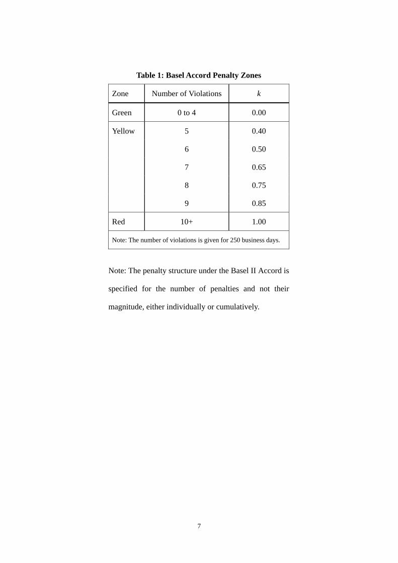
For purposes of the Basel II Accord penalty structure for violations arising from

excessive risk taking, a violation is penalized according to its cumulative frequency of

occurrence in 250 working days, and is given in Table 1.

A violation is defined as follows:

6

Definition: A violation occurs when >tVaR negative returns at time t.

As encouraged by the Basel II Accord, the optimization problem facing ADIs, with

the number of violations and forecasts of risk as endogenous choice variables, is as

follows:

{ }tVARk, Minimize ( )

⎭⎬⎫

⎩⎨⎧ −+−= −160

______

VaR ,VaR3max tt kDCC , (1)

where DCC = daily capital charges,

tVAR = Value-at-Risk for day t,

tttt zYVAR σˆ ⋅−= ,

60

______

VaR = mean VaR over the previous 60 working days,

tY = estimated return at time t,

tz = 1% critical value at time t,

tσ = estimated volatility at time t,

10 ≤≤ k is a violation penalty (see Table 1).

As tY is typically difficult to predict, and as tz is unlikely to change significantly

especially on a daily basis), changes in tσ are crucial for modelling VaR. Substantial

7

Table 1: Basel Accord Penalty Zones

Zone Number of Violations k

Green 0 to 4 0.00

Yellow 5 0.40

6 0.50

7 0.65

8 0.75

9 0.85

Red 10+ 1.00

Note: The number of violations is given for 250 business days.

Note: The penalty structure under the Basel II Accord is

specified for the number of penalties and not their

magnitude, either individually or cumulatively.

8

-10

-8

-6

-4

-2

0

2

4

6

1998 1999 2000 2001 2002 2003 2004

Portfolio Returns VARMA-GARCH

Figure 10: Realized Returns and VARMA-GARCH VaR Forecasts

Note: This is Figure 10 in McAleer and da Veiga (2008a).

9

research has been undertaken in recent years to develop univariate and multivariate

models of volatility, under the conditional, stochastic and realized volatility

frameworks, in order to estimate tσ . Although VaR may also be estimated directly

using regression quantiles (see, for example, Engle and Manganelli (2002)), this

approach is not as popular as modelling volatility and then calculating VaR.

Although considerable research has been undertaken on higher-order moments,

especially in the context of conditional volatility models, these are not considered in

the paper. Model uncertainty for univariate and multivariate processes is also not

considered (see Pesaran, Schleicher and Zaffaroni (2008) for an analysis of model

averaging techniques for portfolio management).

As discussed above, the amendment to the Basel Accord was designed to reward

institutions with superior risk management systems. For testing performance, a

backtesting procedure, whereby the realized returns are compared with the VaR

forecasts, was introduced to assess the quality of a bank’s internal model. In cases

where the internal models lead to a greater number of violations than could

reasonably be expected, given the confidence level, the bank is required to hold a

higher level of capital (see Table 1 for the penalties imposed under the Basel Accord).

If a bank’s VaR forecasts are violated more than nine times in any financial year (see

Table 1), the bank may be required to adopt the standard approach. As discussed in

McAleer and da Veiga (2008b), the imposition of such a penalty is severe as it affects

the profitability of the bank directly through higher daily capital charges, has a

damaging effect on the bank’s reputation, and may lead to the imposition of a more

10

stringent external model to forecast VaR thresholds, which would have the result of

increasing daily capital charges for ADIs.

It should be noted that DCC is to be minimized, with k and tVAR as endogenous

choice variables. [The acronym DCC should be distinguished from a widely used

multivariate conditional volatility model, which will be discussed below.]

It is worth giving a caveat with respect to the minimization of daily capital charges in

times of extreme financial fluctuations, such as the period starting in September 2008.

When excessive risk is very high, and is changing dramatically on a daily basis, daily

capital charges should still be minimized, but sensible portfolio management may

involve greater access to cash after VaR and daily capital charges have been

determined.

3. Data

The data used in the empirical applications in McAleer and da Veiga (2008a, 2008b),

and given as portfolio returns in Figure 10 above, are daily prices measured at 16:00

Greenwich Mean Time (GMT) for four international stock market indexes, namely

S&P500 (USA), FTSE100 (UK), CAC40 (France), and SMI (Switzerland). All prices

are expressed in US dollars. The data were obtained from DataStream for the period 3

August 1990 to 5 November 2004. At the time the data were collected, this period was

the longest for which data on all four variables were available.

The synchronous returns for each market i at time t )( itR are defined as:

11

, , 1log( / )it i t i tR P P −= ,

where tiP , is the price in market i at time t, as recorded at 16:00 GMT.

For the empirical analysis, it was assumed that the portfolio weights are equal and

constant over time, although both of these assumptions can easily be relaxed. The

various conditional volatility models were used to estimate the variance of the

portfolio directly for the single index model, and to estimate the conditional variances

and correlations of all assets and asset pairs to calculate the variance of the portfolio

for the portfolio model. Apart from the Standardized Normal and RiskmetricsTM

models, all the conditional volatility models were estimated under the assumption that

the distribution of the unconditional shocks was (1) normal; and (2) t, with 10 degrees

of freedom.

The empirical results will be discussed further in the context of the last two

Commandments, but the following points should be highlighted:

(i) There is a trade-off between the number of violations and daily capital

charges, with a higher number of violations leading to a higher penalty and

lower daily capital charges through lower VaR.

(ii) Apart from Standardized Normal, which does not estimate any parameters,

and RiskmetricsTM , where the parameters are calibrated rather than estimated,

the number of violations is higher for single index models than for their

portfolio model counterparts, and the mean daily capital charges are

correspondingly higher.

12

(iii) The use of the t distribution with 10 degrees of freedom always leads to

fewer violations, and hence higher mean daily capital charges, for both the

single index and portfolio models.

The two curves in Figure 10, as reproduced below, represent daily returns on the

portfolio of the four aggregate indexes, as well as the forecast VaR thresholds using

the VARMA-GARCH model of Ling and McAleer (2003). From the figure, it can be

seen clearly that there are very few violations, which could mean one or more of the

following:

(1) the volatility model provides an accurate measure of risk and VaR;

(2) the volatility model provides a conservative measure of risk and VaR;

(3) the number of violations is not being used as an endogenous choice

variable.

4. Regression Models and Volatility Models

The purpose of a (linear) regression model is to explain the conditional mean, or first

moment, of tY :

ttt XY εβα ++= , (2)

such that

( ) ttt XXYE βα += ,

13

where α and β are taken to be scalar parameters for convenience.

The purpose of a (univariate) volatility model is to explain the variance, or second

moment, of tY in (2):

ttt hηε = , )1,0(~ iidtη (3)

where tε is the unconditional shock to the variable of interest, tY (typically, a stock

return in empirical finance), which thereby has a risk component, tη is the

standardized residual (namely, a riskless shock, or fundamental), and th denotes

volatility (or risk). One of the primary purposes in modeling volatility is to determine

th to enable tη to be calculated from the observable returns shock, tε . The

volatility, th , may be latent or observed (though it is also likely to be subject to

measurement error).

In the class of conditional volatility models, which are widely used for analysing

monthly, weekly and daily data (though they can also be used for hourly data), th is

modelled as:

12

1 −− ++= ttt hh βαεω , (4)

where there are (typically sufficient) conditions on the parameters ,,, βαω to

ensure that conditional volatility, th , is positive. The specification for th in (4) is

the widely used generalized autoregressive conditional heteroskedasticity, or

GARCH(1,1), model of Engle (1986) and Bollerslev (1986). As the model is

14

conditional on the information set at time t-1, current shocks do not affect th . For

recent surveys of univariate and multivariate conditional volatility models, see Li,

Ling and McAleer (2002), McAleer (2005a), and Bauwens, Laurent and Rombouts

(2006).

Stochastic volatility models can incorporate leverage directly through the negative

correlation between the returns and subsequent volatility shocks (see, in particular,

Zhang, Mykland and Aït-Sahalia (2005), Aït-Sahalia, Mykland and Zhang (2006), and

Barndorff-Nielsen, Hansen, Lunde Shephard (2008)). For a recent review of a wide

range of stochastic volatility models, see Asai, McAleer and Yu (2006).

Realized volatility models can incorporate leverage as this is not explicitly excluded

in the specification. However, realized volatility models are typically not specified to

incorporate leverage.

At the multivariate level, it is not entirely clear how to define leverage in the context

of conditional, stochastic or realized volatility models (for further details, see

McAleer and Medeiros (2008a)).

5. Ten Reasons for Modelling Time-varying Variances, Covariances and

Correlations Using High and Ultra High Frequency Data

Regression models are used to explain the conditional first moment of tY when it is

not constant. Similarly, volatility models are used to explain the second moment of tY

when it is not constant. It is well known that neither the first nor second moments of

tY is constant, especially in the case of financial returns data.

15

Ten reasons for modelling time-varying variances, covariances and correlations using

high frequency (namely, monthly, weekly, daily and hourly) and ultra high frequency

(namely, minute and second) data are as follows:

(1) Volatility from high frequency data can be aggregated, whereas aggregated data at

low frequencies typically display no volatility;

(2) Enables prediction of uncertainty regarding the imposition of tourism taxes on

international tourist arrivals;

(3) Enables prediction of uncertainty regarding the imposition of environmental taxes

on polluters;

(4) Enables prediction of risk in finance;

(5) Enables the prediction of dynamic correlations for constructing financial

portfolios;

(6) Enables the computation of dynamic confidence intervals;

(7) Enables the computation of dynamic Value-at-Risk (VaR) thresholds;

(8) Enables the computation of dynamic confidence intervals for dynamic VaR

thresholds;

(9) Enables the prediction of dynamic variances and covariances for constructing

dynamic VaR thresholds for financial portfolios;

(10) Enables the derivation of a strategy for optimizing dynamic VaR.

6. The Ten Commandments for Optimizing Value-at-Risk and Daily Capital

Charges

Credit risk is the most important type of risk in terms of monetary value, while market

16

risk is typically concerned with stocks and bonds, and related financial derivatives, as

well as exchange rates and interest rates. Operational risk involves credit and market

risk, as well as other operational aspects or risk.

For market, credit and operational risk, choose wisely from:

(C1) Conditional, stochastic and realized volatility.

(C2) Symmetry, asymmetry and leverage.

(C3) Dynamic correlations and dynamic covariances.

(C4) Single index and portfolio models.

(C5) Parametric, semiparametric and nonparametric models.

(C6) Estimation, simulation and calibration of parameters.

(C7) Assumptions, regularity conditions and statistical properties.

(C8) Accuracy in calculating moments and forecasts.

(C9) Optimizing threshold violations and economic benefits.

(C10) Optimizing private and public benefits of risk management.

The commandments progress from the theoretical to the practical. The remainder of

this section briefly discusses each self-explanatory commandment.

(C1) Choose Wisely from Conditional, Stochastic and Realized Volatility

Different volatility models provide different estimates and forecasts of risk, while

different data frequencies lead to different choices of volatility model.

(i) Conditional volatility, which is typically used to model monthly and daily

17

data, is latent (see Li, Ling and McAleer (2002) and Bauwens, Laurent and

Rombouts (2006) for recent reviews). The ease of computation, even for

some multivariate models, as well as its availability in several widely used

econometric software packages, has made this class of models very

popular.

(ii) Stochastic volatility is typically use to model and forecast daily data, and

is also latent (see Asai, McAleer and Yu (2006) for a recent review of

multivariate stochastic volatility models). A distinct advantage of

stochastic volatility models is the incorporation of leverage, at least at the

univariate level. However, the computational burden can be quite severe,

especially for multivariate processes. Moreover, standard econometric

software packages do not yet seem to have incorporated stochastic

volatility algorithms.

(iii) Realized volatility is observable, but is subject to measurement error (see

McAleer and Medeiros (2008a) for a recent review). Such models are used

to calculate observed volatility using tick data. The generated realized

daily volatility measures are then typically modelled using a wide variety

of long memory or fractionally integrated time series processes. It should

be emphasized that microstructure noise (or measurement error) is a

standard problem that arises where realized volatility is used as an estimate

of daily integrated volatility.

(C2) Choose Wisely from Symmetry, Asymmetry and Leverage

Distinguish carefully between asymmetry and leverage, and models that incorporate

asymmetry and leverage, either by construction or through the use of parametric

18

restrictions.

Asymmetry is a straightforward concept, but leverage seems to be the subject of much

misunderstanding in practice.

Definition: Asymmetry captures the different impacts of positive and negative

shocks of equal magnitude on volatility.

Definition: Leverage captures the effects of negative (positive) shocks of equal

magnitude on increasing (decreasing) the debt-equity ratio, thereby increasing

(decreasing) subsequent volatility and risk (see Black (1976)).

Thus, leverage is a special case of asymmetry, with volatility decreasing progressively

as returns shocks change progressively from negative to positive.

It follows that symmetry is the absence of asymmetry, including leverage. The widely

used ARCH and GARCH models are symmetric.

Several popular models of volatility display asymmetry, though not necessarily

leverage. For example, the GJR model of Glosten, Jagannathan and Runkle (1992) is

asymmetric but does not display leverage (see McAleer, Hoti and Chan (2008) for a

multivariate extension of the asymmetric GJR model, VARMA-AGARCH), while the

EGARCH model of Nelson (1991) is asymmetric and can display leverage, depending

on the signs of the coefficients relating to the size and sign effects.

In the context of stochastic volatility models, leverage is imposed through a negative

19

correlation between returns and subsequent volatility shocks. There are many

alternative types of asymmetry at the univariate and multivariate levels (see, for

example, Asai and McAleer (2005, 2008c) and McAleer and Medeiros (2008b)).

Although realized volatility models may be modified to incorporate both intra- and

inter-day leverage, this does not seem to have been accomplished to date.

Extensions of leverage to multivariate processes are somewhat more difficult.

(C3) Choose Wisely between Dynamic Correlations and Dynamic Covariances

Covariances and correlations are used to model relationships between pairs of assets

for portfolio risk management:

Correlations are used in the construction of a portfolio. Consider two financial assets,

X and Z:

(a) correlation (X,Z) +1 specialize on the asset with the higher

historical and/or expected returns;

(b) correlation (X,Z) -1 hedge (or diversify);

(c) correlation (X,Z) 0 need to balance risk and returns.

On the other hand, dynamic variances and covariances are used to calculate the VaR

of a given portfolio.

As a multivariate extension of equation (3), consider the relationship between

20

covariances and correlations, as follows:

tttt DDQ Γ= ,

(5)

in which tQ is the conditional covariance matrix, tΓ is the conditional correlation

matrix, and tD is the diagonal matrix of conditional standard deviations, namely

ith , where

1,2

1, −− ++= tiitiiiit hh βεαω ,

and i= 1,…,m is the number of assets in the portfolio.

The matrix tQ is used to calculate VaR forecasts, while the matrix tΓ is used to

construct and update portfolios.

It should be emphasized that tQ can be modelled directly, as in the BEKK model of

Engle and Kroner (1995), or indirectly through modelling tΓ , and using (5), such as

using the dynamic conditional correlation (DCC) model of Engle (1992), of which the

constant conditional correlation (CCC) model of Bollerslev (1990) is a special case

(for an application of the scalar BEKK versus indirect DCC models, see Caporin and

McAleer (2008)).

The BEKK model is given as follows:

21

''' 1'

11 BBQAAQQQ tttt −−− ++= εε , (6)

where BAQQt ,,, are m dimensional matrices. It is clear that the specification in (6)

guarantees a positive definite covariance matrix. However, as the dimensions of the

three parameter matrices, namely BAQ ,, , are the same as for tQ , a computational

difficulty can arise frequently in the BEKK model of tQ as it suffers from the

so-called “curse of dimensionality” in having far too many parameters.

It follows from (5) that

11 −−=Γ tttt DQD , (7)

so that tΓ can be modelled directly, or indirectly through modelling tQ . A

parsimonious model of tΓ is given in the DCC model, as follows:

12'

1,1,121 )1( −−− Γ++−−=Γ ttitit θηηθθθ , (8)

where 21, θθ are scalar parameters. As the specification does not guarantee that the

elements along the main diagonal are all unity, and all of the off-diagonal terms lie in

the range [-1, 1], Engle (2002) standardizes the matrix in (8) so that the elements

satisfy the definition of a conditional correlation.

22

Although the DCC model is parsimonious in terms of parameters, a common

empirical finding, especially for stock indexes, is that the long run conditional

correlation matrix is constant (namely, 1,0 21 == θθ ), with the outcome being that

news has little practical effect in changing the purportedly dynamic conditional

correlations. This is not altogether surprising as, apart from the positive diagonal

elements in a matrix version of DCC (see, for example, the GARCC model of

McAleer, Chan, Hoti and Lieberman (2008)), the off-diagonal terms of the coefficient

matrix can be positive or negative. The imposition of an unrealistic constraint that all

the elements of the matrix are the same constant has the effect of making 1θ very

close to zero and 2θ very close to unity, especially for a portfolio with a large

numbers of assets. This practical problem associated with DCC is alleviated with

various extensions of the the model, such as GARCC.

Dynamic correlations have recently been developed for multivariate stochastic

volatility models using the Wishart distribution (see Asai and McAleer (2008b)), but

the computational burden can be quite severe.

To date there does not seem to have been any research undertaken on modelling the

dynamic correlations for pairs of standardized residuals for multivariate realized

volatility models.

(C4) Choose Wisely between Index and Portfolio Models

Estimation and forecasting of VaR thresholds of a portfolio requires estimation and

forecasting the variance and covariances of portfolio returns. Volatility models can be

used to estimate the variance of portfolio returns either by (1) fitting a univariate

23

volatility model to the portfolio returns (hereafter called the single index model (see

McAleer and da Veiga (2008a, 2008b)); or (2) using a multivariate volatility model to

forecast the conditional variance of each asset in the portfolio to calculate the

forecasted portfolio variance (hereafter called the portfolio model). Asai and McAleer

(2008b) have extended the idea of a portfolio index model to a multivariate GARCH

process.

The central issue is the signal to noise ratio. Single index models require only a

univariate model to calculate the variance of the single index, and hence require no

covariances or correlations. There is little signal, but there is also little noise. Portfolio

models have a lot of signal because of all the pairs of covariances and correlations,

but there is also a lot of noise in the estimated parameters or coefficients.

As an illustration in the case of two assets, let ttt zxy )1( λλ −+= ,

where

ty = single index return to the portfolio of two assets,

tx = return to financial asset, tX

tz = return to financial asset, tZ

tt zx )1( λλ −+ = portfolio return on two assets,

12

1 −− ++= ytyytyyyt hh βεαω

24

12

1 −− ++= xtxxtxxxt hh βεαω

12

1 −− ++= ztzztzzzt hh βεαω

111 −−− ++= xztxzztxtxzxzxzt hh βεεαω .

As the two conditional variances and single covariance are estimated, it follows that:

xztztxtyt hhhh )1(2)1( 22 λλλλ −+−+≠ ,

even though

),cov()1(2)var()1()var()var( 22ttttt zxzxy λλλλ −+−+= .

Therefore, the single index and portfolio approaches can lead to different results when

the time-varying variances and covariances are estimated.

The number of covariances increases dramatically with m, the number of assets in the

portfolio. Thus, for m = 2, 3, 4, 5, 10, 20, 30, 40, 50, 100, the number of covariances

is 1, 3, 6, 10, 45, 190, 435, 780, 1225 and 4950, respectively. This increases the

computational burden significantly, unless some structure can be imposed to increase

parsimony.

(C5) Choose Wisely from Parametric, Semiparametric and Nonparametric Models

Conditional volatility is latent, and conditional volatility models are typically

25

semiparametric or parametric.

Stochastic volatility is latent, and stochastic volatility models are typically parametric.

Realized volatility is observable, and realized volatility models are nonparametric.

Each type of model typically has an optimal method of estimation, as follows:

(1) Conditional volatility models are typically estimated by the maximum

likelihood (ML) method when the standardized residuals are normally distributed, or

by the quasi-maximum likelihood (QML) method when they are not normal (for

further details, see Li, Ling and McAleer (2002) or Bauwens, Laurent and Rombouts

(2006);

(2) Stochastic volatility models are typically estimated by the Bayesian Markov

Chain Monte Carlo (MCMC), Monte Carlo Likelihood (MCL), Empirical Likelihood

(EL), or Efficient Method of Moments (EMM) methods (for further details, see Asai,

McAleer and Yu (2006));

(3) Realized volatility models are typically estimated by nonparametric methods

(for detailed analyses, see Zhang, Mykland and Aït-Sahalia (2005), Aït-Sahalia,

Mykland and Zhang (2006), and Barndorff-Nielsen, Hansen, Lunde Shephard (2008);

for recent reviews of the literature, see Bandi and Russell (2007) and McAleer and

Medeiros (2008a)).

(C6) Choose Wisely from Estimation, Simulation and Calibration of Parameters

26

RiskmetricsTM calibrates the parameters in both univariate and multivariate models,

and hence is concerned with forecasting volatility. As there are no estimated

parameters, there are no standard errors, and there can be no inference.

Conditional volatility models are concerned with estimation and forecasting. The

statistical properties of consistency and asymptotic normality for univariate and

multivariate conditional volatility models are now well established in the literature

(see, for example, Ling and McAleer (2002a, 2002b, 2003)).

Stochastic volatility models are concerned with simulation and forecasting. As the

Bayesian MCMC, MCL, EL or EMM methods are typically used for estimation, the

small sample or asymptotic properties of the estimators are well known.

Realized volatility models are based on nonparametric estimation methods, and their

asymptotic properties are well known. Large samples are typically required for the

use of nonparametric methods. In analyzing ultra high frequency tick data on financial

returns, very large samples are usually available.

(C7) Choose Wisely from Assumptions, Regularity Conditions and Statistical Properties

It is essential to distinguish between assumptions and regularity conditions that are

derived from the assumptions of the underlining model.

Assumptions are required to obtain the moment conditions (otherwise known as

regularity conditions), especially the second and fourth moments, as well as

27

log-moments. Moment conditions are required to obtain the statistical properties of

consistency and asymptotic normality, thereby also providing diagnostic checks of the

model.

The regularity conditions for univariate and multivariate GARCH models are now

well known in the literature. The log-moment conditions for GARCH(1,1) and

GJR(1,1) were established by Lee and Hansen (1994) and McAleer, Chan and

Marinova (2007), respectively, and the second and fourth moments for the

multivariate extensions of GARCH and GJR, namely the VARMA-GARCH and

VARMA-AGARCH models, by Ling and McAleer (2003) and McAleer, Hoti and

Chan (2008)). The statistical properties of BEKK were established by Jeantheau

(1998) and Comte and Lieberman (2003), and for a generalization of DCC, namely

the Generalized Autoregressive Conditional Correlation (GARCC) model, by

McAleer, Chan, Hoti and Lieberman (2008).

The Bayesian statistical properties of the univariate and multivariate stochastic

volatility models are well known, as they are also for realized volatility models.

(C8) Choose Wisely between Accuracy in Calculating Moments and Forecasts

Derive appropriate measures to determine the accuracy of estimates and forecasts,

including economic benefits, and evaluate dynamic checks of second moments and

log-moment conditions for univariate and multivariate conditional volatility models.

The moment and log-moment conditions should be calculated as diagnostic checks of

the underlying volatility models. The second moment conditions for univariate

28

GARCH and GJR are straightforward to calculate, but the log-moments are typically

not calculated. The corresponding moment and log-moment conditions for

multivariate processes are typically ignored in practice. Moment conditions are not

necessary for the EGARCH model as it is a function of the standardized residuals

rather than the unconditional returns shocks.

Typically, only the second moment conditions for univariate ARCH and GARCH

models are checked, despite the ease of computing the log-moment conditions for

GARCH(1,1) and GJR(1,1) (see Lee and Hansen (1994) and McAleer, Chan and

Marinova (2007), respectively.

The accuracy of estimating models of the respective underlying processes should be

weighed against any improvements in forecasting performance.

(C9) Choose Wisely between Optimizing Threshold Violations and Economic

Benefits

As the daily capital charge is to be minimized with respect to both k and VaR, when

the estimated volatility increases, the penalty from violation (k) tends to decrease,

while VaR increases, with the end result being that capital charges increase.

Similarly, when the estimated volatility decreases, the penalty from violation (k) tends

to increase, while VaR decreases, with the end result being that capital charges

decrease.

Therefore, daily capital charges should be minimized, and economic benefits should

29

be maximized, using k and VaR as an endogenous decision variables.

Tables 2 and 3 make it clear that increasing the number of violations leads to lower

mean daily capital charges across all the volatility models considered, and for both the

single index and portfolio approaches.

The Basel II penalty structure would seem to be too lenient for violations, especially

for large violations, as the penalty structure focuses on the number, rather than the

number and magnitude, of violations in (1).

A strategy to minimize daily capital charges has been devised by McAleer,

Jiménez-Martin and Peréz-Amaral (2008), with k and VaR as endogenous choice

variables. The strategy seems to work much better than treating k as exogenous.

In short, there is a need to change the penalty structure under the Basel Accord,

otherwise there is likely to be continuing excessively high risk taking.

(C10) Choose Wisely between Optimizing Private and Public Benefits of Risk

Management

In summary, ADIs should balance violations (which may be crucial to avoid for public

relations purposes) against daily capital charges.

As the regulations stand at present, the Basel II Accord would seem to encourage risk

taking as the penalties for violations are exceedingly low, and hence would seem to

favour violations rather than managing and monitoring excessive risk taking (see

30

Tables 2 and 3).

It is essential to determine whether increasing the number of violations, which

subsequently leads to lower mean daily capital charges, is in the public interest in

terms of monitoring and managing excessive risk and VaR.

There is an urgent requirement to balance risk taking with prudent self regulation or

government regulation in the banking and finance industry (as seen earlier in the 2003

remarks by Alan Greenspan). There may, in fact, be moral hazard in self regulation in

the banking and finance industry, as qualified by Greenspan in 2003, especially in

terms of federal guarantees of private debt.

The financial meltdown in September and October 2008 (and still counting) demands

more careful and responsible regulation of the industry.

7. Concluding Remarks

The largely self-regulated management of excessive risk taking in the world of

banking and finance has led to the worst financial disaster in September-October 2008

since the market collapse of 1929. Government and private regulation of credit risk,

which is the most important type of risk in terms of monetary value, and market risk,

which is typically concerned with stocks and bonds, related financial derivatives, and

exchange rates and interest rates, have been found to be largely inadequate.

This paper analysed market risk management and monitoring under the Basel II

Accord, and presented the optimization problem facing authorized deposit-taking

31

institutions. Ten reasons for modelling time-varying variances, covariances and

correlations using high and ultra high frequency data were given, and the Ten

Commandments for optimizing Value-at-Risk (VaR) and daily capital charges were

analysed. As the Basel II Accord would seem to encourage risk taking at the

expense of providing accurate measures and forecasts of risk and VaR, the paper gave

some idiosyncratic suggestions and guidelines regarding how improvements might be

made regarding optimal strategies for risk monitoring and management, especially

when there is a strong and understandable movement into holding and managing cash

than in dealing with risky financial investments.

8. Epilogue

“Rules are made to be broken.” Anonymous “Ignore all rules.” Anonymous “One of the quickest ways to break something is to fix it when it ain’t broken.” Anonymous Butch Cassidy: “Every day you get older. Now that’s a law.” Butch Cassidy and the Sundance Kid Etta Place: “Do you know what you’re doing?” Butch Cassidy: “Theoretically.” Butch Cassidy and the Sundance Kid

32

Commandments, laws, rules, regulations, guidelines, codes, call them what you will.

They are all made to be ignored and/or broken. The frequency of breaking

commandments may be testament to the indefatigability of human beings to ignore

the blindingly obvious, or to the blindingly obvious fact that such commandments

may not always be particularly useful.

The fact remains that commandments are routinely ignored, for whatever reason. The

Ten Commandments for organizing a conference (McAleer (1997)), for attending a

conference (McAleer and Oxley (2001), for presenting a conference paper (McAleer

and Oxley (2002), for ranking university quality (McAleer (2005b)), and for

academics (McAleer and Oxley (2005)), are frequently downloaded (using download

statistics) and read, but are also frequently ignored, although the financial penalties

are not quite as frightening as when the Ten Commandments for optimizing VaR and

daily capital charges are broken.

33

Table 2: Mean Daily Capital Charge and AD of Violations for the Single Index Model

AD of Violations

Model

Number of Violations

Mean Daily Capital Charge Maximum Mean

Standardized Normal 35 12.329 3.506 0.631

RiskmetricsTM 27 9.113 2.772 0.456

ARCH 62 8.319 2.758 0.552

ARCH-t 36 8.832 2.302 0.551

GARCH 34 8.095 2.430 0.464

GARCH-t 14 8.981 2.302 0.441

GJR 34 8.095 2.430 0.464

GJR-t 13 9.903 1.701 0.521

PGARCH 31 8.041 1.205 0.362

PGARCH-t 9 9.034 1.708 0.510

EGARCH 30 7.968 1.154 0.298

EGARCH-t 9 8.986 1.556 0.489

Notes:

(1) The daily capital charge is given as the negative of (3+k) times the greater of the previous day’s VaR or the

average VaR over the last 60 business days, where k is the violation penalty.

(2) AD is the absolute deviation of the violations from the VaR forecast.

Note: This is Table 8 in McAleer and da Veiga (2008b). The models are as follows: ARCH was developed by Engle (1982), GARCH by Bollerslev (1986), GJR by Glosten, Jagannathan and Runkle (1992), EGARCH by Nelson (1991), and PGARCH is the asymmetric power GARCH model of Ding, Granger and Engle (1993).

34

Table 3: Mean Daily Capital Charge and AD of Violations for the Portfolio Model

AD of Violations

Model

Number of Violations

Mean Daily Capital Charge Maximum Mean

Standardized Normal 36 12.916 3.509 0.617

RiskmetricsTM 28 8.509 2.516 0.413

ARCH 19 9.132 2.271 0.540

ARCH-t 9 10.581 1.691 0.463

CCC 7 9.685 2.125 0.498

CCC-t 1 11.498 1.489 1.489

GJR 7 9.724 1.657 0.505

GJR-t 2 11.571 0.857 0.549

EGARCH 6 9.692 1.566 0.466

EGARCH-t 2 11.544 0.727 0.482

PGARCH 6 9.787 1.485 0.472

PGARCH-t 2 11.658 0.623 0.490

VARMA-GARCH 6 9.760 1.974 0.454

VARMA-GARCH-t 1 11.633 1.287 1.287

PS-GARCH 7 10.700 1.902 0.442

PS-GARCH-t 1 11.833 1.321 1.321

Notes:

(1) The daily capital charge is given as the negative of (3+k) times the greater of the previous day’s VaR or

the average VaR over the last 60 business days, where k is the violation penalty.

(2) AD is the absolute deviation of the violations from the VaR forecast.

Note: This is Table 9 in McAleer and da Veiga (2008b). In addition to the models described in the note to Table 2, the models are as follows: CCC was developed by Bollerslev (1990), VARMA-GARCH by Ling and McAleer (2003), and PS-GARCH by McAleer and da Veiga (2008a).

35

References Aït-Sahalia, Y., P.A. Mykland and L. Zhang (2006), Ultra high Frequency Volatility

Estimation with Dependent Microstructure Noise, Working Paper, w11380, NBER.

Asai, M. and M. McAleer (2005), Dynamic Asymmetric Leverage in Stochastic

Volatility Models, Econometric Reviews, 24, 317-332. Asai, M. and M. McAleer (2008a), A Portfolio Index GARCH Model, International

Journal of Forecasting, 24, 449-461. Asai, M. and M. McAleer (2008b), The Structure of Dynamic Correlations in

Multivariate Stochastic Volatility Models, to appear in Journal of Econometrics. Asai, M. and M. McAleer (2008c), Alternative Asymmetric Stochastic Volatility

Models, to appear in Econometric Reviews. Asai, M., M. McAleer and J. Yu (2006), Multivariate Stochastic Volatility: A Review,

Econometric Reviews, 25, 145-175. Bandi, F.M. and J.R. Russell (2007), Volatility Estimation, in J.R. Birge and V. Linetsky

(eds.), Handbook of Financial Engineering, Elsevier, Amsterdam. Barndorff-Nielsen, O.E., P.H. Hansen, A. Lunde and N. Shephard (2008),

Subsampling realised kernels, to appear in Econometrica. Basel Committee on Banking Supervision, (1988), “International Convergence of

Capital Measurement and Capital Standards”, BIS, Basel, Switzerland. Basel Committee on Banking Supervision, (1995), “An Internal Model-Based

Approach to Market Risk Capital Requirements”, BIS, Basel, Switzerland. Basel Committee on Banking Supervision, (1996), “Supervisory Framework for the

Use of “Backtesting” in Conjunction with the Internal Model-Based Approach to Market Risk Capital Requirements”, BIS, Basel, Switzerland.

Bauwens, L., S. Laurent and V.K. Rombouts (2006), Multivariate GARCH: A Survey,

36

Journal of Applied Econometrics, 21, 79-109. Black, F. (1976), Studies of Stock Market Volatility Changes, in 1976 Proceedings of

the American Statistical Association, Business and Economic Statistics Section, pp. 177-181.

Bollerslev, T. (1986), Generalised Autoregressive Conditional Heteroscedasticity,

Journal of Econometrics, 31, 307-327. Bollerslev, T. (1990), Modelling the Coherence in Short-run Nominal Exchange Rates:

A Multivariate Generalized ARCH Approach, Review of Economics and Statistics, 72, 498-505.

Caporin, M. and M. McAleer (2008), Scalar BEKK and Indirect DCC, Journal of

Forecasting, 27, 537-549. Comte, F. and O. Lieberman (2003), Asymptotic Theory for Multivariate GARCH

Processes, Journal of Multivariate Analysis, 84, 61-84. Ding, Z., C.W.J. Granger and R.F. Engle (1993), A Long Memory Property of Stock

Market Returns and a New Model, Journal of Empirical Finance, 1, 83-106. Engle, R.F. (1982), Autoregressive Conditional Heteroscedasticity with Estimates of

the Variance of United Kingdom Inflation, Econometrica, 50, 987-1007. Engle, R.F. (2002), Dynamic Conditional Correlation: A Simple Class of Multivariate

Generalized Autoregressive Conditional Heteroskedasticity Models, Journal of Business and Economic Statistics, 20, 339-350.

Engle, R.F. and K.F. Kroner (1995), Multivariate Simultaneous Generalized ARCH,

Econometric Theory, 11, 122-150. Engle, R.F. and S. Manganelli (2002), .CAViaR: Conditional Autoregressive Value at

Risk by Regression Quantiles, Journal of Business and Economic Statistics, 22, 367-381.

Glosten, L.R., R. Jagannathan and D.E. Runkle (1992), On the Relation Between the

Expected Value and Volatility of the Nominal Excess Return on Stocks, Journal

37

of Finance, 46, 1779-1801. Jeantheau, T. (1998), Strong Consistency of Estimators for Multivariate ARCH

Models, Econometric Theory, 14, 70-86. Jorion, P. (2000), Value at Risk: The New Benchmark for Managing Financial Risk,

McGraw-Hill, New York. Lee, S.W. and B.E. Hansen (1994), Asymptotic Theory for the GARCH(1,1)

Quasi-Maximum Likelihood Estimator, Econometric Theory, 10, 29-52. Li, W.K., S. Ling and M. McAleer (2002), Recent Theoretical Results for Time Series

Models with GARCH Errors, Journal of Economic Surveys, 16, 245-269. Reprinted in M. McAleer and L. Oxley (eds.), Contributions to Financial Econometrics: Theoretical and Practical Issues, Blackwell, Oxford, 2002, pp. 9-33.

Ling, S. and M. McAleer (2002a), Necessary and Sufficient Moment Conditions for

the GARCH(r,s) and Asymmetric Power GARCH(r,s) Models, Econometric Theory, 18, 722-729.

Ling, S. and M. McAleer (2002b), Stationarity and the Existence of Moments of a

Family of GARCH Processes, Journal of Econometrics, 106, 109-117. Ling, S. and M. McAleer (2003), Asymptotic Theory for a Vector ARMA-GARCH

Model, Econometric Theory, 19, 278-308. McAleer, M. (1997), The Ten Commandments for Organizing a Conference, Journal

of Economic Surveys, 11, 231-233. McAleer, M. (2005a), Automated Inference and Learning in Modeling Financial

Volatility, Econometric Theory, 21, 232-261. McAleer, M. (2005b), The Ten Commandments for Ranking University Quality,

Journal of Economic Surveys, 19, 649-653. McAleer. M., F. Chan, S. Hoti and O. Lieberman (2008), Generalized Autoregressive

Conditional Correlation, Econometric Theory, 24, 1554-1583.

38

McAleer, M., F. Chan and D. Marinova (2007), An Econometric Analysis of

Asymmetric Volatility: Theory and Application to Patents, Journal of Econometrics, 139, 259-284.

McAleer, M., S. Hoti and F. Chan (2008), Structure and Asymptotic Theory for

Multivariate Asymmetric Conditional Volatility, to appear in Econometric Reviews.

McAleer. M., J.-Á. Jiménez-Martin and T. Peréz-Amaral (2008), A Strategy for

Minimizing Daily Capital Charges for Value-at-Risk, unpublished paper, Department of Economics, Complutense University of Madrid, Spain.

McAleer. M. and M.C. Medeiros (2008a), Realized Volatility: A Review, Econometric

Reviews, 27, 10-45. McAleer. M. and M.C. Medeiros (2008b), A Multiple Regime Smooth Transition

Heterogeneous Autoregressive Model for Long Memory and Asymmetries, Journal of Econometrics, 147, 104-119.

McAleer, M. and L. Oxley (2001), The Ten Commandments for Attending a

Conference, Journal of Economic Surveys, 15, 671-678. McAleer, M. and L. Oxley (2002), The Ten Commandments for Presenting a

Conference Paper, Journal of Economic Surveys, 16, 215-218. McAleer, M. and L. Oxley (2005), The Ten Commandments for Academics, Journal

of Economic Surveys, 19, 823-826. McAleer, M. and B. da Veiga (2008a), Forecasting Value-at-Risk with a Parsimonious

Portfolio Spillover GARCH (PS-GARCH) Model, Journal of Forecasting, 27, 1-19.

McAleer, M. and B. da Veiga (2008b), Single Index and Portfolio Models for

Forecasting Value-at-Risk Thresholds, Journal of Forecasting, 27, 217-235. Nelson, D. (1991), Conditional Heteroskedasticity in Asset Returns: A New Approach,

Econometrica, 59, 347-370.

39

Pesaran, M.H., C. Schleicher and P. Zaffaroni (2008), Model Averaging in Risk

Management with an Application to Futures Markets, to appear in Journal of Empirical Finance.

RiskmetricsTM (1996), J.P. Morgan Technical Document, 4th edition, New York. J.P.

Morgan. Zhang, L., P.A. Mykland and Y. Aït-Sahalia (2005), A Tale of Two Time Scales:

Determining Integrated Volatility with Noisy High Frequency Data, Journal of the American Statistical Association, 100, 1394 – 1411.