Embed Size (px)
Citation preview

The stiffness and strength of the gyroid lattice
S. N. Khaderi1 , V. S. Deshpande2 , N. A. Fleck3
Department of Engineering, Cambridge University, Cambridge
Abstract
Recently, a nanoscale lattice material, based upon the gyroid topology has been self-
assembled by phase separation techniques (Scherer et al. Advanced Materials, v24, p1217,
2012) and prototyped in thin film applications. The mechanical properties of the gyroid
are reported here. It is a cubic lattice, with a connectivity of three struts per joint, and is
bending-dominated in its elasto-plastic response to all loading states except for hydrostatic:
under a hydrostatic stress it exhibits stretching-dominated behaviour. The three indepen-
dent elastic constants of the lattice are determined through a unit cell analysis using the
finite element method; it is found that the elastic and shear modulus scale quadratically
with the relative density of the lattice, whereas the bulk modulus scales linearly. The plastic
collapse response of a rigid, ideally plastic gyroid lattice is explored using the upper bound
method, and are validated by finite element calculations for an elastic-ideally plastic lat-
tice. The effect of geometrical imperfections, in the form of random perturbations to the
joint positions, is investigated for both stiffness and strength. It is demonstrated that the
hydrostatic modulus and strength are imperfection sensitive, in contrast to the deviatoric
response. The macroscopic yield surface of the imperfect lattice is adequately described by
a modified version of Hill’s anisotropic yield criterion. The article ends with a case study on
the stress induced within a gyroid thin film, when the film and its substrate are subjected
to a thermal expansion mismatch.
Keywords: Gyroid lattice; Lattice materials; Foams;
[email protected]@[email protected]
Preprint submitted to International Journal of Solids and Structures April 5, 2013

1. Introduction
Lattice materials are micro-architectured porous solids, and can be manufactured with
a broad range of micro-structures and length scales. They can be random or periodic, and
open or closed-cell. Examples include foams, the octet truss, hollow truss, gyroid, Kagome
and honeycomb (Deshpande et al., 2001b; Jacobsen et al., 2007; Queheillalt and Wadley,
2005; Fleck et al., 2010; Cote et al., 2004; Scherer et al., 2012). Their mechanical properties
(for example stiffness, strength and fracture toughness) depend upon the properties of the
parent material from which the lattice is made, upon the relative density ρ̄ (density of the
lattice/density of the solid) and the topology that defines the lattice. When a macroscopic
strain is applied to a lattice, it can deform either by bending or stretching of the struts.
A bending-dominated lattice has a low strength and stiffness compared to a stretching-
dominated lattice for the same ρ̄ (Deshpande et al., 2001a; Ashby, 2006; Gibson and Ashby,
1997). It is the nodal connectivity, Z, (i.e. the number of struts joining at a node) that
determines whether the lattice deforms in a bending or stretching-dominated mode. In 3D,
the elastic modulus of a foam (for which Z=3-4) scales quadratically with the ρ̄, whereas the
elastic modulus of an octet truss lattice ( for which Z=12) scales linearly with ρ̄ (Deshpande
et al., 2001b). In contrast, the fracture toughness of the lattice need not depend upon the
fracture toughness of the parent material (Fleck and Qiu, 2007).
Lattice materials have potential for thin films in electrical application. For example, films
of thickness on the micron scale and comprising the gyroid lattice have been manufactured by
phase separation techniques (Scherer et al., 2012). Possible applications include displays (by
employing electrochromism) and electrodes for solar cells. The successful use of such devices
will inevitably require a knowledge of the mechanical properties of such gyroid lattices. This
motivates the current study: our aim is to determine the stiffness and strength of the gyroid
lattice in both its ideal, periodic state and in an imperfect state where the nodes are randomly
displaced.
2

Figure 1: (a) The gyroid minimal surface. (b) Gyroid lattice obtained by in-filling one side of the surface.
1.1. The gyroid lattice
Formally, the gyroid is a triply periodic minimal surface4 (with zero mean curvature),
and was identified by Alan Schonen in 1970 (Schoen, 1970). It belongs to the cubic space
group Ia3̄d (see Fig. 1(a)). Filling the space on one side of the surface leads to a porous solid
of volume fraction equal to 0.5. It has the topology of an open-celled foam and is sketched
in Fig. 1(b). The equations defining the gyroid involve elliptical integrals and can be found
elsewhere (Schoen, 1970; Gandy and Klinowski, 2000). A close approximation to the gyroid
is given by (Wohlgemuth et al., 2001; Lambert et al., 1996)
F (x, y, z) = t, (1)
where,
F (x, y, z) = sin
(
2πx
a
)
cos
(
2πy
a
)
+ sin
(
2πy
a
)
cos
(
2πz
a
)
+ sin
(
2πz
a
)
cos
(
2πx
a
)
, (2)
4Other minimal surfaces exist such as Weaire-Phelan structure, Kelvin foam, Schwarz P and D surfaces.
3

a is the periodicity of the gyroid and t = 0. A companion family of gyroid-like surfaces,
with a constant mean curvature is defined in (Grosse-Brauckmann and Meinhard, 1996) and
(Grosse-Brauckmann, 1997). These surfaces belong to the cubic space group I4132 and are
defined by F (x, y, z) = t, where −1.5 ≤ t ≤ 1.5. A number of closely related gyroid lattices
can be defined as follows. Choose a length scale a.
(i) For t < 0 and space in-filling according to F < −t defines a gyroid with ρ̄ < 0.5 (see
Fig. 2(a)).
(ii) Now take t > 0. In-filling for F > t produces a gyroid of opposite chirality to that in
(i).
(iii) The two gyroids (i) and (ii) are inter-penetrating lattices, and together form the double
gyroid, of space group Ia3̄d.
(iv) Fill the void in (iii) and then remove the double gyroid. The remaining structure is
the inverse gyroid.
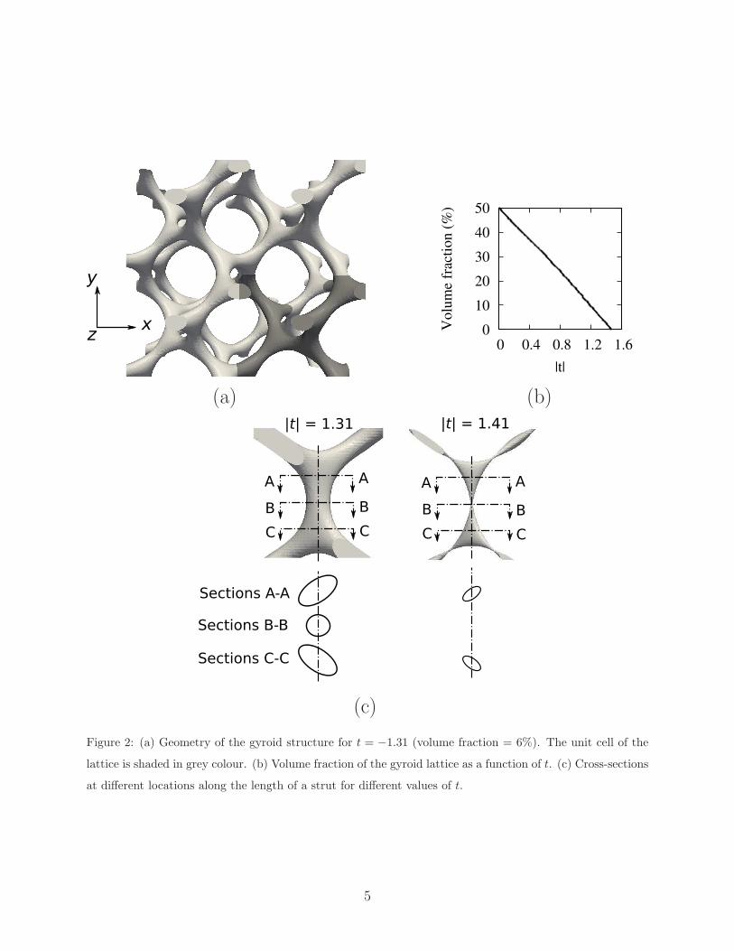
The gyroid has a connectivity of three struts per node. The cross-section of the struts
of the gyroid changes from an elliptical shape near the Plateau borders to a circular shape
at the midspan (see Fig. 2(c)). The principal directions of the elliptical cross section jump
discontinuously at midspan (see Fig. 2(c)). At large absolute values of t, most of the material
is present at the Plateau borders. The value |t| = 1.41 is the limiting case, as the area of
the circular cross-section at midspan vanishes.
1.2. Observed gyroids
The gyroid morphology has been observed in many physical systems. For example,
when strontium-saturated soaps are annealed at 230 ◦C, self-assembly of the lipids results
in a double gyroid network of strontium ions embedded in a hydrocarbon matrix (Luzzati
and Spegt, 1967). The double gyroid (DG) morphology also appears during the phase
separation of diblock copolymers (see the review by Matsen and Bates (1996)). At high
temperatures the block co-polymers exist as a disordered homogeneous solution; at low
temperatures they phase separate/self assemble to form a variety of morphologies, which
include lamellar, cylindrical, spherical and DG. The lowest energy configuration of these
4
x
y
z
(a)
0
10
20
30
40
50
0 0.4 0.8 1.2 1.6
Volu
me
frac
tion (
%)
|t|
(b)
A
B
C
A
B
C
|t| = 1.31
Sections A-A
Sections B-B
Sections C-C
A
B
C
A
B
C
|t| = 1.41
(c)
Figure 2: (a) Geometry of the gyroid structure for t = −1.31 (volume fraction = 6%). The unit cell of the
lattice is shaded in grey colour. (b) Volume fraction of the gyroid lattice as a function of t. (c) Cross-sections
at different locations along the length of a strut for different values of t.
5

competing morphologies depends upon the volume fraction of each phase of the block co-
polymers, interfacial energy and the entropic stretching energy of the polymer chains. The
single gyroid network has been observed in the scales of butterfly wings. Michielsen and
Stavenga (2008) compared the TEM images of the cross section of the scale of a butterfly
wings with three different cubic micro-structures. They found that the gyroid lattice is
the best fit to the TEM micro-structure. Saranathan et al. (2010) used small angle X-ray
scattering to reveal that the micro-structure of the butterfly wings comprises the single gyroid
lattice (unit cell size ≈ 300 nm). They also studied the optical properties of the gyroid lattice
using photonic band gap modelling. Almsherqi et al. (2012) have shown that mitochondria
of the retinal cone cells of tree shrew consist of the 8-12 parallel layers of gyroid surfaces
(unit cell size ≈ 400 nm) that function as multi-focal lens, interference filter and wave guide.
On a macroscale, Yan et al. (2012) have fabricated macroscopic single gyroid lattices
(unit cell sizes between 2 and 8 mm of relative density of 15 %) from stainless steel powder
using laser sintering technique. They also measured the stress-strain response of the gyroid
lattices. As their main objective was to evaluate the laser sintering method to fabricate
lattice materials, an extensive study on the mechanical properties was not performed.
Recently, Scherer et al. (2012) have shown that the annealing of poly(4-fluorostyrene-
r-styrene)-b-poly(d,l-lactide) (P(F)S-b-PLA) results in a DG network of PLA embedded in
styrene matrix. They successfully replaced the PLA with vanadium pentoxide and etched
out the styrene matrix to obtain a DG of vanadium pentoxide (unit cell size ≈ 40 nm). This
DG has potential for application in electrochromic devices.
Except for the work of Yan et al. (2012), very little is known about the mechanical
properties of gyroid lattice and this is the subject of the present paper. We report on the
elastic properties and multi-axial strength of the single gyroid lattice using both analytical
and numerical techniques.
The paper is organised as follows. We first perform a unit cell analysis of the three-
dimensional gyroid lattice, as defined by (1), by employing the finite element (FE) method.
The elastic constants and the yield strength in the cubic directions are thereby obtained. At
low relative density, the gyroid lattice is idealised as 3D framework of beams, of uniform cross
section. The accuracy of this approximation is evaluated for both stiffness and strength. The
6

yield surface of the gyroid (approximated by the framework of cylindrical beams) is calcu-
lated analytically by the upper bound method and verified using finite element simulations.
The effect of geometric imperfection on the elasto-plastic properties of the gyroid is then
investigated: the nodes are moved in a random manner to generate imperfect gyroids. An
analytical expression for the multi-axial yielding of the imperfect gyroid is proposed, and
is employed in a case study on the yielding of a thin film, when subjected to a thermal
expansion mismatch with the underlying substrate.
2. Elastic and yield responses of the gyroid lattice
The effective elastic-plastic properties are calculated using a periodic unit cell of size
a × a × a (see the shaded struts in Fig. 2(a)). The gyroid geometry is created using the
isosurface and isocaps command in Matlab (http://www.mathworks.co.uk), which is then
output as a steriolithographic (STL) file. The STL file is used to create a solid three-
dimensional finite element (FE) mesh of linear tetrahedra using the mesh generation software
Engrid (http://engits.eu /en/engrid). This mesh is used to perform unit cell analysis using
the finite element package ABAQUS (www.simulia.com). All FE simulations reported in
this work are based on small strain approximation.
The unit cell, aligned with the Cartesian axes (x, y, z), is subjected to periodic boundary
conditions, such that the relative displacement ∆ui of periodic nodes of the FE mesh is given
by ∆ui = ǫij∆Xj, in terms of an imposed macroscopic strain ǫij, and the relative position
of the periodic nodes in the jth direction ∆Xj. The resulting macroscopic stress, σij, is
obtained from the reaction forces on the periodic nodes and is given by
σij =1
2a3
∑
J
(
∆XiFJj +∆XjF
Ji
)
, (3)
where F Jj are the reaction forces on the node J , and summation is performed on all boundary
nodes.
2.1. Elastic properties
The material of the gyroid lattice is assumed to be isotropic with an elastic modulus ES
and Poisson’s ratio νS = 0.3. As the gyroid lattice has cubic symmetry (with x, y and z as
7
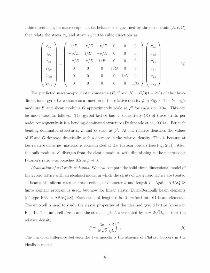
cubic directions), its macroscopic elastic behaviour is governed by three constants (E, ν,G)
that relate the stress σij and strain ǫij in the cubic directions as
ǫxx
ǫyy
ǫzz
2ǫyz
2ǫxz
2ǫxy
=
1/E −ν/E −ν/E 0 0 0
−ν/E 1/E −ν/E 0 0 0
−ν/E −ν/E 1/E 0 0 0
0 0 0 1/G 0 0
0 0 0 0 1/G 0
0 0 0 0 0 1/G
σxx
σyy
σzz
σyz
σxz
σxy
. (4)
The predicted macroscopic elastic constants (E,G and K = E/3(1 − 2ν)) of the three-
dimensional gyroid are shown as a function of the relative density ρ̄ in Fig. 3. The Young’s
modulus E and shear modulus G approximately scale as ρ̄2 for (ρ/ρs) > 0.04. This can
be understood as follows. The gyroid lattice has a connectivity (Z) of three struts per
node; consequently, it is a bending-dominated structure (Deshpande et al., 2001a). For such
bending-dominated structures, E and G scale as ρ̄2. At low relative densities the values
of E and G decrease drastically with a decrease in the relative density. This is because at
low relative densities, material is concentrated at the Plateau borders (see Fig. 2(c)). Also,
the bulk modulus K diverges from the elastic modulus with diminishing ρ̄: the macroscopic
Poisson’s ratio ν approaches 0.5 as ρ̄→ 0.
Idealisation of cell walls as beams. We now compare the solid three-dimensional model of
the gyroid lattice with an idealised model in which the struts of the gyroid lattice are treated
as beams of uniform circular cross-section, of diameter d and length L. Again, ABAQUS
finite element program is used, but now for linear elastic Euler-Bernoulli beam elements
(of type B33 in ABAQUS). Each strut of length L is discretised into 64 beam elements.
The unit-cell is used to study the elastic properties of the idealised gyroid lattice (shown in
Fig. 4). The unit-cell size a and the strut length L are related by a = 2√2L, so that the
relative density
ρ̄ =3π
16√2
(
d
L
)2
. (5)
The principal difference between the two models is the absence of Plateau borders in the
idealised model.
8

10-5
10-4
10-3
10-2
10-1
10-2
10-1
ρ_
K/Es
G/Es
E/Es
2
1
0.2
Figure 3: Elastic constants of the gyroid lattice as a function of the relative density.
The results of the unit cell analysis are shown in Fig. 5. The expressions for the elastic
constants obtained by curve fitting are given below:
E
Es
= 0.465ρ̄2,
G
Es
= 0.331ρ̄2,
K
Es
=1
9ρ̄,
(6)
where E, G and K are the uniaxial, shear and bulk modulus of the lattice, respectively.
As the gyroid lattice is bending-dominated, the elastic and shear modulus have a quadratic
dependence on the relative density, as already noted from Fig. 3. Note from Eqn (6) that the
bulk modulus has a linear dependence on relative density, signifying that under hydrostatic
loading the beam elements stretch. Consequently, K/E → ∞ as ρ̄ → 0, implying that the
Poisson’s ratio ν approaches 0.5 as ρ̄→ 0.
The elastic, shear and bulk modulus obtained from the beam and solid models are com-
pared in Fig. 6. The difference in response by the two models is primarily due to the effect of
Plateau borders: present in the solid model, but absent in the beam model. Similar features
have been noted previously for the hexagonal honeycomb, see Simone and Gibson (1998).
9

6
137 17
2
8
14
3
4 12
15
10
136
14
8
7
17 16
2
9
5
3
4
12
11 1
zy 5
4
16
14 12
2
13
15
8
7
17
111
6
9
3
10 10
9
5
16
1
11
xy
xz
15
1
2
3
4
5
6
7
8
9
10
11
12
13
14
15
16
17
x
y
z
a
a
a
L
Figure 4: Different views of the unit-cell of the beam model for the gyroid lattice. The struts are labelled as
shown.
10

10-6
10-5
10-4
10-3
10-2
10-3
10-2
10-1
ρ_
E/ES
K/ES
G/ES
Figure 5: Elastic constants of the gyroid lattice obtained using the beam model.
10-5
10-4
10-3
10-2
10-1
10-2
10-1
ρ_
K/Es
E/Es
G/Es
0.2
Solid model
Beam model
Figure 6: Comparison of elastic constants obtained from the solid and beam models for the gyroid lattice.
11

10-5
10-4
10-3
10-2
10-1
10-2
10-1
σYσS
ρ_
0.2
Solid, FE
Beam, FE
Beam, analytical
(a)
10-4
10-3
10-2
10-1
10-2
10-1
σhYσS
ρ_
0.2
Solid, FE
Beam, FE
Beam, analytical
(b)
Figure 7: Comparison of (a) uniaxial yield strength and (b) hydrostatic yield strength obtained from the
solid and beam models for the gyroid lattice.
2.2. Yield Behaviour
The lattice is made from an isotropic, elastic, ideally plastic solid of modulus ES, Poisson’s
ratio νS = 0.3, yield strain ǫS = 0.01 and a yield strength σS = 0.01ES in accordance with
J2 flow theory5. We take the macroscopic flow strength to be attained, when the maximum
component of macroscopic strain attains the value 10ǫY , where the macroscopic yield strain
is approximately given by ǫY = σS/ES
√ρ̄, see Gibson and Ashby (1997).
The macroscopic uniaxial yield strength in cubic directions (σY ) and hydrostatic yield
strength (σhY ), as obtained by finite element simulations, are compared for both the full
solid and beam models in Fig. 7. The solid model is slightly stronger than the beam model
at high relative density, with the converse result at low relative density. We conclude that
the beam model is adequate in the range 4% < ρ̄ < 15%, and in the remainder of the paper
we shall employ the beam model.
5For computational reasons, the material is endowed with a very small strain hardening, as specified by
a tangent modulus h = 10−4ES .
12
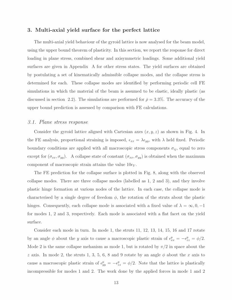
3. Multi-axial yield surface for the perfect lattice
The multi-axial yield behaviour of the gyroid lattice is now analysed for the beam model,
using the upper bound theorem of plasticity. In this section, we report the response for direct
loading in plane stress, combined shear and axisymmetric loadings. Some additional yield
surfaces are given in Appendix A for other stress states. The yield surfaces are obtained
by postulating a set of kinematically admissible collapse modes, and the collapse stress is
determined for each. These collapse modes are identified by performing periodic cell FE
simulations in which the material of the beam is assumed to be elastic, ideally plastic (as
discussed in section 2.2). The simulations are performed for ρ̄ = 3.3%. The accuracy of the
upper bound prediction is assessed by comparison with FE calculations.
3.1. Plane stress response
Consider the gyroid lattice aligned with Cartesian axes (x, y, z) as shown in Fig. 4. In
the FE analysis, proportional straining is imposed, ǫxx = λǫyy, with λ held fixed. Periodic
boundary conditions are applied with all macroscopic stress components σij , equal to zero
except for (σxx, σyy). A collapse state of constant (σxx, σyy) is obtained when the maximum
component of macroscopic strain attains the value 10ǫY .
The FE prediction for the collapse surface is plotted in Fig. 8, along with the observed
collapse modes. There are three collapse modes (labelled as 1, 2 and 3), and they involve
plastic hinge formation at various nodes of the lattice. In each case, the collapse mode is
characterised by a single degree of freedom φ, the rotation of the struts about the plastic
hinges. Consequently, each collapse mode is associated with a fixed value of λ = ∞, 0,−1
for modes 1, 2 and 3, respectively. Each mode is associated with a flat facet on the yield
surface.
Consider each mode in turn. In mode 1, the struts 11, 12, 13, 14, 15, 16 and 17 rotate
by an angle φ about the y axis to cause a macroscopic plastic strain of ǫpxx = −ǫpzz = φ/2.
Mode 2 is the same collapse mehanism as mode 1, but is rotated by π/2 in space about the
z axis. In mode 2, the struts 1, 3, 5, 6, 8 and 9 rotate by an angle φ about the x axis to
cause a macroscopic plastic strain of ǫpyy = −ǫpzz = φ/2. Note that the lattice is plastically
incompressible for modes 1 and 2. The work done by the applied forces in mode 1 and 2
13

y
x
Mode 3
2
4
7
9
16
38
10 5
Mode 1
15
17
16
11
12
13
14
ϕ
x
z
ϕ
Mode 2
yz
ϕ
Plastic
hinges
(a)
-1
-0.5
0
0.5
1
-2 -1.5 -1 -0.5 0 0.5 1
σσ
Y
yy
σxx /σY
Mode
1
Mode
1
Mode 2
Mode 2
Mod
e 3
Mod
e 3
ζ=1.76
Perfect, ζ=0
Analytical
FE
(b)
Figure 8: Yield behaviour in (σxx, σyy) space. (a) Deformed geometry (solid lines) and location of plastic
hinges for different modes of collapse. The dashed lines show the initial inclination of the struts. (b)
Analytical and FE predictions of the yield surfaces with an indication of different modes of plastic collapse.
The FE results are shown for perfect (ζ = 0) and imperfect lattice with ζ = 1.76.
14
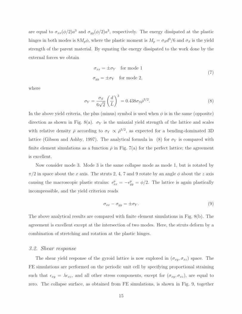
are equal to σxx(φ/2)a3 and σyy(φ/2)a
3, respectively. The energy dissipated at the plastic
hinges in both modes is 8Mpφ, where the plastic moment is Mp = σSd3/6 and σS is the yield
strength of the parent material. By equating the energy dissipated to the work done by the
external forces we obtain
σxx = ±σY for mode 1
σyy = ±σY for mode 2,(7)
where
σY =σS
6√2
(
d
L
)3
= 0.438σS ρ̄3/2. (8)
In the above yield criteria, the plus (minus) symbol is used when φ is in the same (opposite)
direction as shown in Fig. 8(a). σY is the uniaxial yield strength of the lattice and scales
with relative density ρ̄ according to σY ∝ ρ̄3/2, as expected for a bending-dominated 3D
lattice (Gibson and Ashby, 1997). The analytical formula in (8) for σY is compared with
finite element simulations as a function ρ̄ in Fig. 7(a) for the perfect lattice; the agreement
is excellent.
Now consider mode 3. Mode 3 is the same collapse mode as mode 1, but is rotated by
π/2 in space about the x axis. The struts 2, 4, 7 and 9 rotate by an angle φ about the z axis
causing the macroscopic plastic strains: ǫpxx = −ǫpyy = φ/2. The lattice is again plastically
incompressible, and the yield criterion reads
σxx − σyy = ±σY . (9)
The above analytical results are compared with finite element simulations in Fig. 8(b). The
agreement is excellent except at the intersection of two modes. Here, the struts deform by a
combination of stretching and rotation at the plastic hinges.
3.2. Shear response
The shear yield response of the gyroid lattice is now explored in (σxy, σxz) space. The
FE simulations are performed on the periodic unit cell by specifying proportional straining
such that ǫxy = λǫxz, and all other stress components, except for (σxy, σxz), are equal to
zero. The collapse surface, as obtained from FE simulations, is shown in Fig. 9, together
15
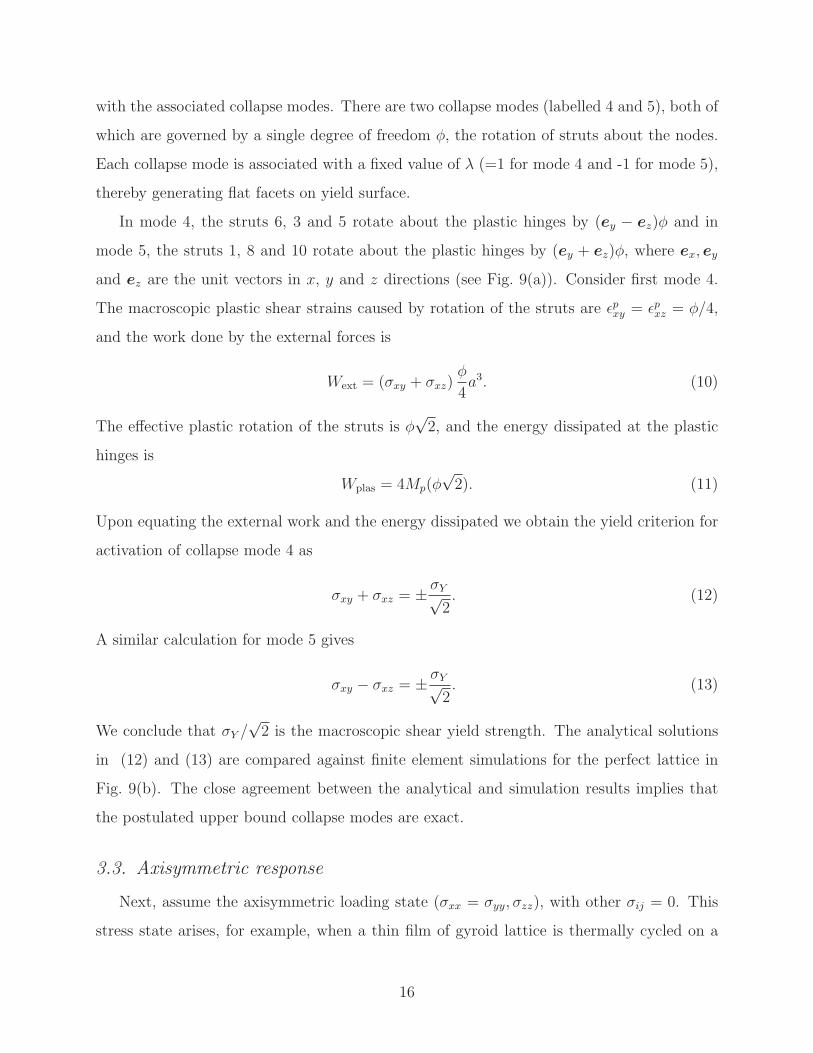
with the associated collapse modes. There are two collapse modes (labelled 4 and 5), both of
which are governed by a single degree of freedom φ, the rotation of struts about the nodes.
Each collapse mode is associated with a fixed value of λ (=1 for mode 4 and -1 for mode 5),
thereby generating flat facets on yield surface.
In mode 4, the struts 6, 3 and 5 rotate about the plastic hinges by (ey − ez)φ and in
mode 5, the struts 1, 8 and 10 rotate about the plastic hinges by (ey + ez)φ, where ex, ey
and ez are the unit vectors in x, y and z directions (see Fig. 9(a)). Consider first mode 4.
The macroscopic plastic shear strains caused by rotation of the struts are ǫpxy = ǫpxz = φ/4,
and the work done by the external forces is
Wext = (σxy + σxz)φ
4a3. (10)
The effective plastic rotation of the struts is φ√2, and the energy dissipated at the plastic
hinges is
Wplas = 4Mp(φ√2). (11)
Upon equating the external work and the energy dissipated we obtain the yield criterion for
activation of collapse mode 4 as
σxy + σxz = ± σY√2. (12)
A similar calculation for mode 5 gives
σxy − σxz = ± σY√2. (13)
We conclude that σY /√2 is the macroscopic shear yield strength. The analytical solutions
in (12) and (13) are compared against finite element simulations for the perfect lattice in
Fig. 9(b). The close agreement between the analytical and simulation results implies that
the postulated upper bound collapse modes are exact.
3.3. Axisymmetric response
Next, assume the axisymmetric loading state (σxx = σyy, σzz), with other σij = 0. This
stress state arises, for example, when a thin film of gyroid lattice is thermally cycled on a
16

y
x
1
3
4
5
6
8
9
10
11
12
13
14
15
y
x
1
3
4
5
6
8
9
10
11
12
13
14
15
Mode 4 Mode 5
1617 1617
zx
1
11
12
54
16
17
3
86
13
10
1415
ϕ
ϕ 1
11
12
5
4
16
17
86
13
10
14 15
3
ϕ
ϕ
zx
ϕ ϕ
ϕ
ϕ
ϕ
ϕ
Plastic
hinges
(a)
-0.5
0
0.5
1
-1 -0.5 0 0.5 1
σσ
Y
xz
σxy /σY
Mode 4
Mode 4 Mode 5
Mode 5
FE,ζ=1.76
Analytical
Perfect, FE
(b)
Figure 9: Yield behaviour in (σxy, σxz) space. (a) Deformed geometry (solid lines) of gyroid and the locations
of plastic hinges for different modes of collapse. (b) Comparison of analytical yield surface with FE predictions
for the perfect (ζ = 0) and imperfect gyroid with ζ = 1.76.
17

substrate, with the unit normal to the free surface of the film aligned with the cubic z direc-
tion. The FE simulations are performed on the periodic unit cell by imposing proportional
straining such that ǫzz = λǫxx, and the so-obtained yield surface is given in Fig. 10 along
with the collapse mode (labelled as mode 6). The collapse mode consists of combined plastic
rotation and axial stretching at nodes. It is instructive to consider two extreme cases. (1)
When σxx = σzz, the lattice is in a state of hydrostatic stress, and the beam elements deform
by axial stretching (as noted above for the elastic case). (2) When σzz = 0, the lattice is in
a state of plane stress, where the lattice deforms both by a combination of hinge rotation
and stretching, as noted above.
In the single collapse mode for axisymmetric loading, all struts except 2, 4, 7 and 8
yield plastically (see Fig. 10(a)). The collapse mode can be described by two degrees of
freedom: the axial extension ǫL/2 and rotation φ of the struts at the plastic hinges. Here, ǫ
is a dimensionless kinematic variable characterising the degree of axial stretch. The collapse
mode results in the following macroscopic plastic strains: ǫpxx = ǫpyy = (ǫ+φ)/2 and ǫpzz = ǫ−φ.Note that the extensional degree of freedom leads to dilatation of the unit cell, whereas the
rotational degree of freedom results in a volume-preserving plastic strain. The work done by
the external forces is
Wext(ǫ, φ) = a3 (σxx(ǫ+ φ) + σzz(ǫ− φ)) .
The energy dissipated is given by
Wplas(ǫ, φ) = 16ǫL
2Pp(ξ) + 16φMp(ξ), (14)
where the plastic collapse force is Pp(ξ) = σSd2(
sin−1 ξ + ξ√
1− ξ2)
/2 and the plastic
collapse moment is Mp(ξ) = σSd3 (1− ξ2)
3/2/6. The neutral axis of bending/stretching of
the plastic hinge is located at ξr, above the mid-plane of circular section (of radius r). A
straightforward kinematic argument gives ξ = (L/2r)(ǫ/φ). When |ξ| > 1, the neutral axis
is located outside the beam with Mp = 0.
Now use the upper bound theorem and note that φ and ǫ are independent. Then, the
macroscopic yield surface of the lattice for axisymmetric loading is obtained in parametric
18

form as
σxx =σY2
[
3
2
(
L
d
)
(
sin−1 ξ + ξ√
1− ξ2)
±(
1− ξ2)3/2
]
,
σzz = −σY2
[
−3
2
(
L
d
)
(
sin−1 ξ + ξ√
1− ξ2)
±(
1− ξ2)3/2
]
,
(15)
where −1 ≤ ξ ≤ 1. Upon making the choice ξ = 1 in (15), the hydrostatic limit is attained
such that each direct stress is of magnitude
σhY =1
3σS ρ̄. (16)
Note that the hydrostatic strength scales linearly with the relative density ρ̄, implying that
the lattice deforms by axial stretching. This value of σhY is compared with FE simulations
in Fig. 7(b); the agreement is excellent. The yield criterion as defined in (15) is exact for a
rigid, ideally plastic solid and is confirmed by comparison with FE simulations in Fig. 10(b)
for the perfect lattice. Recall that the uniaxial yield strength σY scales as ρ̄3/2, thus the
yield surface in Fig. 10(b) is increasingly elongated with diminishing ρ̄.
Elastic buckling – The above analysis assumes that the gyroid lattice plastically collapses
under hydrostatic loading. An alternative possible collapse mode is elastic buckling. An
elastic eigenvalue analysis has been performed using the FE software ABAQUS for the beam
model. The simulations (not shown) reveal that the hydrostatic buckling strength is
σbuckling =1
13Esρ̄
2. (17)
The switch in mechanism from plastic collapse to buckling occurs when the relative density
ρ̄ satisfies
ρ̄ =13
3ǫS,
where ǫS = σS/ES is the uniaxial yield strain of the parent material. Recall that ǫS is
on the order of 1 − 10% for polymers, and so elastic buckling can occur for such lattices
at realistic values of relative density. We note in passing that elastic bifurcation from the
undeformed state can only occur under pure hydrostatic compression of the gyroid, see
Chen et al. (1999). No bifurcations from the initial state are possible for the imperfect
gyroid considered subsequently for any stress states.
19

y
x
2
4
7
9
ϕ
ϕ ϕ
ϕ
ϕ
ϕϕ
ϕ ϕPlastic hinges
Mode 6
(a)
−6 −4 −2 0 2 4 6σxx/σY
−6
−4
−2
0
2
4
6
σzz
σY
Perfect,ζ=0
ζ=1.76,FE
Analytical
FE
(b)
Figure 10: Yield behaviour for axisymmetric loading (σxx = σyy, σzz). (a) Location of plastic hinges when
the gyroid lattice is subjected to an axisymmetric load. (b) Comparison of analytical yield surface with FE
simulations for perfect (ζ = 0) lattice. The yield surface of imperfect lattice is labelled as ζ = 1.76.
4. Effect of imperfections upon the elastic and plastic properties
Practical gyroid lattices contain a range of imperfections from spatial variations in relative
density to missing beam elements and misplaced nodes. The significance of such imperfec-
tions has been explored for both 2D and 3D lattices, see for example (Silva et al., 1995; Chen
et al., 1999; Zhu et al., 2000). We observe that the gyroid lattice shares several features with
the 2D honeycomb: under deviatoric loading, the response is bending dominated whereas
under hydrostatic loadings the beam elements stretch. For such lattices, the hydrostatic
strength is much more imperfection-sensitive than the deviatoric strength. Is this a feature
of the gyroid lattice too? In order to address this, the sensitivity of the elastic and plastic
responses of the gyroid lattice is explored for the case where each node is displaced by a
fixed distance ζd in a random direction, where d is the strut diameter and the imperfection
magnitude ζ is taken to lie in the range of 0-2.
A FE analysis is performed on a periodic, representative volume element (RVE) con-
taining N1/3 unit cells along each of the Cartesian (x, y, z) axes. A convergence study is
performed to determine the magnitude of the RVE that gives accurate macroscopic values
20

0.8
0.9
1
1.1
0 50 100 150 200 250
N
E/EP
σY/σPY
Figure 11: Dependence of the elastic modulus and yield strength of an imperfect gyroid on the number of
cells (N) used for ζ = 0.353. (•)P refers to quantities of the perfect lattice.
for the elastic and plastic responses. Accordingly, the elastic modulus E and uniaxial yield
strength σY , as obtained from FE simulations, are plotted for various values of N in Fig. 11,
for ζ = 0.353. In the figure, E and σY of the imperfect lattice are normalised by the re-
sponses of an ideal lattice (denoted by the superscript P ). For each value of N , 5 random
realizations are used. It can be seen that the results are independent of N provided N ≥ 64.
In the following we adopt this value for N .
4.1. Imperfection sensitivity
An assessment of the imperfection sensitivity of the main elastic and plastic properties
of the lattice is now given. The Young’s modulus E, shear modulus G and bulk modulus
K (in material axes aligned with the Cartesian reference frame) are given in Fig. 12(a) for
the choice ρ̄ = 3.3% and imperfection ζ in the range 0-1.76. Likewise, the uniaxial yield
strength σY , shear yield strength τY and hydrostatic yield strength σhY are plotted as a
function of ρ̄ in Fig. 12(b). The values of E, G, σY and τY are almost insensitive to the
level of imperfection ζ, whereas the bulk modulus K and the hydrostatic yield strength σhY
are extremely imperfection sensitive. This can be explained as follows. The deformation
mode changes from stretching to bending when a small imperfection is introduced. The
21

0
2
4
6
8
0 0.5 1 1.5
ζ
K/EP
E/EP
G/EP
(a)
0
1
2
3
4
5
0 0.5 1 1.5
ζ
σY/σYP
σhY /σYP
τY/σYP
(b)
Figure 12: (a) Elastic constants and (b) yield strengths of the ρ̄ = 3.3% gyroid lattice as a function of the
imperfection magnitude ζ. (•)P refers to quantities of the perfect lattice.
dependence of K on ρ̄ then changes from linear to quadratic; similarly, the scaling of σhY
changes from linear to 3/2 power.
4.2. Multiaxial yield response of the imperfect lattice
The sensitivity of the shape of the yield surface to imperfection is now explored. We
anticipate a major change in the shape of yield surface in stress space that contains the
hydrostatic limit: σhy drops much more sharply with increasing ζ than does σY or τY . To
illustrate this, we plot the yield surface in axisymmetric stress space (σxx = σyy, σzz) in
Fig. 10(b) for ζ = 0 and ζ = 1.76. The yield surface becomes much less elongated with
increasing ζ. This has been noted previously for irregular hexagonal honeycombs, see for
example (Chen et al., 1999). In contrast, for stress states that generate a bending response of
the perfect lattice, there is only a very minor change in behaviour when nodal imperfections
are introduced. Consequently, the yield surfaces for the plane stress loading (σxx, σyy) and for
shear loading (σxy, σxz) are little changed when ζ is increased from 0 to 1.76, see Figs. 8(b)
and 9(b).
22

5. Analytical formula for the multiaxial yield function
For practical applications, it is beneficial to obtain an expression for the macroscopic
multiaxial yield behaviour of the gyroid lattice in analytic form. We make two attempts to
do this and restrict our attention to the practical case of the imperfect lattice. It is clear from
Fig. 12(b) that the hydrostatic and uniaxial yield strengths converge to a constant values
for ζ > 1.5, and so the multiaxial response for ζ = 1.76 can be taken as representative of
that for large imperfection. All FE simulations in this section are performed for ρ̄ = 3.3%.
5.1. Case A – The Deshpande-Fleck (D-F) foam model
First, we attempt to curve fit the D-F isotropic metal foam model (Deshpande and Fleck,
2000). Recall that the D-F yield function is of the form
σ2e + α2σ2
h = c2, (18)
where σe is the von Mises effective stress, σh is the hydrostatic stress and (α, c) are material
constants. Upon fitting Eqn (18) to the (σhY , σY ), data of Fig. 12(b) at ζ = 1.76, we
obtain α = 3/(2√2) and c = ασY , where σY = 0.315σS ρ̄
3/2 is the uniaxial yield strength
of the imperfect lattice. The accuracy of the resulting D-F yield function is acceptable for
the axisymmetric case, see Fig. 13(a). A second assessment is made in (σh, σxy) space, see
Fig. 13(b). The loading is now σxx = σyy = σzz = σh along with σxy. In this sub-space,
the D-F foam model is conservative by at most 20 %, with most deviation occurring for the
state of pure shear. Recall that the imperfect gyroid is not isotropic, and thus an isotropic
description entails an approximation. We proceed to improve the accuracy of the analytical
description, but at the cost of more fitting parameters.
5.2. Case B – Extension of Hill’s anisotropic yield function
In order to obtain an improved description of the yield behaviour we use the modified
Hill’s yield criterion, as proposed by Deshpande et al. (2001b):
A (σxx − σyy)2 + B (σyy − σzz)
2 + C (σzz − σxx)2 +Dσ2
xy + Eσ2yz + Fσ2
xz +Gσ2h = 1, (19)
23

-1.5
-1
-0.5
0
0.5
1
1.5
-1.5 -1 -0.5 0 0.5 1 1.5
σσ
Y
zz
σxx /σY
Foam andanisotropicyield criteria
AA
(a)
-1
-0.5
0
0.5
1
-1 -0.5 0 0.5 1
σσ
Y
xy
σh /σY
Foam yield criterion
Anisotropic yield criterion
(b)
Figure 13: Comparison between the isotropic foam and anisotropic yield criteria for (a) axisymmetric loading
and (b) in (σh, σxy) space . ‘+’ Symbols refer to finite element simulations of a imperfect lattice (one
realization). In (a), the stress state in a gyroid film subject to thermal stress is marked by label A.
where the constants A to G are obtained by curve fitting, as follows. Consider the imperfect
lattice (ζ = 1.76). The constants A to G are obtained by considering the following loading
states:
i the hydrostatic yield strength σhY is almost identical to the uniaxial yield strength σY
at ζ = 1.76, see Fig. 12(b). Consequently, G = 1/σ2Y .
ii under uniaxial loading in the x, y or z directions, the uniaxial strength σY is obtained.
Consequently, A = B = C = 4/(9σ2Y ).
iii under shear loading in xz, yz or xy plane, we note from Fig. 12(b), that the shear
strength τY = 0.77σY . Consequently, D = E = F = 1.69/σ2Y .
The yield surface, as defined by (19), is compared against simulations in Fig. 13. The
anisotropic yield criterion is more accurate than the isotropic yield criterion for stress states
far from the hydrostatic limit.
We note in passing that the anisotropic yield function collapses to the D-F surface in
the absence of the shear stress components (σxy, σxz, σyz). Thus, for axisymmetric loading
(σxx = σyy, σzz), it offers no improvement over the isotropic version, see Fig. 13(a).
24

6. Case study: the gyroid thin films
The above yield criteria can be used immediately for design purposes. Consider, for
example, the application of the gyroid lattice to electronic displays. A thin film of gyroid
lattice is bonded to a glass substrate, and when infiltrated with a suitable electrolyte, it
functions as an electrochromic device (Scherer et al., 2012). The gyroid is taken to be
imperfect, with ζ = 1.76. In service, the gyroid film may yield due to thermal expansion
mismatch with the underlying substrate or due to swelling of the lattice caused by the
electrochemical reactions within the electrochromic device. Assume that one of the cubic
directions of the gyroid lattice is aligned with the unit normal to the surface, and arbitrarily
take this to be the z direction.
First, consider the thermal problem. Impose a uniform temperature change ∆T to the
film and substrate, from the initial, stress-free configuration. The components of the mis-
match strain are ǫ∗xx = ǫ∗yy = ∆α∆T , where ∆α = αf − αs is the difference in the coefficient
of thermal expansion between the film αf6 and substrate αs. The thermal stresses due to
this mismatch is σxx = σyy = −E∆α∆T/(1− ν), where E is the Young’s modulus and ν is
the Poisson’s ratio of the lattice. From the data shown in Fig. 12(a), we can assume that
E = 0.348ES ρ̄2 and ν = 1/3. This state of stress is marked by points A in Fig. 13(a), for
positive and negative values of ∆α∆T . Both versions of the yield functions as derived in the
previous section imply that the maximum allowable temperature change without inducing
yield is ∆T = 0.78ǫS(1 − ν)/∆α√ρ̄, where ǫS is the yield strain of the solid material. It is
instructive to compare this with the maximum allowable value of ∆T of a solid film, without
inducing yielding. Consider a solid film that is made from the same material as the lattice,
bonded to the substrate, and subjected to the thermal mismatch strain as mentioned above.
The thermal stresses due to this mismatch is σxx = σyy = −ES∆α∆T/(1−νS), where ES and
νS are the Young’s modulus and Poisson’s ratio of the solid film, respectively. Assuming that
the solid film yields according to the von Mises yield criterion, we have ∆T = ǫS(1−νS)/∆α.We conclude that the gyroid can undergo a larger ∆T than its parent solid, for all practical
ρ̄. To emphasize this, table 1 shows ∆T values for solid and gyroid films (ρ̄ = 10%), as-
6αf of the gyroid lattice is equal to the coefficient of thermal expansion of the solid it is made from.
25

Table 1: Maximum allowed temperature change ∆T (to avoid plastic yielding) for gyroids made from different
materials, assuming αs = 9.1× 10⁻⁶ ◦C−1.
Film material ǫS (%)αf
(10−6 ◦C−1)
∆T (◦C) for
solid film
∆T (◦C) for
gyroid film
(ρ̄ = 10 %)
Copper (Ashby, 2005) 0.026 17.1 10 25
Nickel (Ashby, 2005) 0.037 13.3 21 52
Platinum (Smithells, 1984) 0.053 9.2 40 101
Cobalt (Smithells, 1984) 0.117 12.3 65 163
suming that the substrate is made from silica glass αs = 9.1× 10⁻⁶ ◦C−1 (Ashby, 2005) and
νS = 1/3. For all film materials, the gyroid lattice can sustain a larger ∆T than the solid
material by a factor of 2–2.5.
Second, consider the possibility of yielding of the gyroid lattice when it is used as an
electrochromic device. During operation of the electrochromic device, intercalation of ions
from the electrolyte into the struts of the gyroid lattice takes place (Scherer et al., 2012),
and this may result in swelling of the lattice. The components of mismatch strain are
ǫ∗xx = ǫ∗yy = ǫv/3, where the stress-free volumetric strain ǫv depends upon the concentration
of intercalating species in the struts (Zhang et al., 2007). The stress due to constrained
swelling is σxx = σyy = −Eǫv/[3(1 − ν)]. Now apply either of the analytical functions in
(18) and (19) for the imperfect gyroid. We deduce that ǫv is given by ǫv = 2.34ǫS(1−ν)/√ρ̄.
For comparison, consider the intercalation of ions into a solid film, made of the same material
as the lattice, and bonded to the substrate. When subjected to the same mismatch strain as
mentioned above, the in-plane stress due to volumetric swelling is σxx = σyy = −ESǫv/[3(1−νS)]. Upon applying the von Mises yield criterion we obtain ǫv = 3ǫS(1 − νS). A summary
of the allowable volumetric strain is given in table 2 for both solid (assuming νS = 1/3)
and gyroid films (ρ̄ = 10%), made from the same parent materials as introduced in Table
1. Again, the gyroid lattice outperforms the solid thin films. Thus, a gyroid lattice shows
promise for thin film applications. Thermal conductivity is an important parameter in such
26

Table 2: Maximum allowed volume expansion ǫv (to avoid plastic yielding) for gyroids made from different
materials.
Material ǫS (%) ǫv (%) for solid material ǫv (%) for ρ̄ = 10 %
Copper 0.026 0.05 0.12
Nickel 0.037 0.07 0.18
Platinum 0.053 0.11 0.26
Cobalt 0.117 0.23 0.57
applications and this is analysed in Appendix B.
7. Concluding remarks
1. The perfect gyroid lattice has cubic symmetry and deforms by bar stretching under
macroscopic hydrostatic stressing. Consequently, its macroscopic bulk modulus K and
hydrostatic strength σhY scale linearly with the relative density ρ̄. Under all other
stress states, the bars of the lattice bend. Consequently, the Young’s modulus and
shear modulus (aligned with the cubic axes) scale as ρ̄2; and the uniaxial yield strength
σY and shear yield strength τY scale as ρ̄3/2.
2. Imperfections, in the form of a random repositioning of the nodes of the lattice, lead
to a severe knock-down in the hydrostatic properties (elastic and plastic), but to a
negligible change in deviatoric properties. This is traced to the fact that bar bending
occurs for all stress states including hydrostatic. A similar behaviour has been noted
previously by Chen et al. (1999) for the regular hexagonal honeycomb.
3. The yield surface of the perfect and imperfect gyroid has been determined for a broad
range of stress states. A small geometric imperfection reduces the hydrostatic strength
to a value comparable with the uniaxial strength. The yield surface of the imperfect
lattice (ζ = 1.76) can be fitted by a quadratic yield criterion, such as Deshpande-Fleck
isotropic foam model or the modified Hill anisotropic yield criterion. The anisotropic
criterion is more accurate, but it requires additional calibration.
4. The thermo-mechanical properties of a gyroid thin film upon an elastic substrate are
assessed for application to electronic displays. It is demonstrated that the lattice can
27

sustain a relatively large temperature excursion and swelling strain without inducing
yield, when compared to a solid film made from the same material.
References
Almsherqi, Z., Margadant, F., Deng, Y., 2012. A look through lens cubic mitochondria.
Interface Focus.
Ashby, M. F., 2005. Material selection in mechanical design. Elsevier.
Ashby, M. F., 2006. The properties of foams and lattices. Philosophical Transactions of the
Royal Society A 364, 15 – 30.
Chen, C., Lu, T., Fleck, N., 1999. Effect of imperfections on the yielding of two-dimensional
foams. Journal of the Mechanics and Physics Solids 47, 2235 – 2272.
Cote, F., Deshpande, V., Fleck, N., Evans, A., 2004. The out-of-plane compressive behavior
of metallic honeycombs. Materials Science and Engineering: A 380, 272 – 280.
Deshpande, V., Ashby, M., Fleck, N., 2001a. Foam topology: bending versus stretching
dominated architectures. Acta Materialia 49 (6), 1035 – 1040.
Deshpande, V., Fleck, N., 2000. Isotropic constitutive models for metallic foams. Journal of
the Mechanics and Physics of Solids 48 (6), 1253–1283.
Deshpande, V., Fleck, N., Ashby, M., 2001b. Effective properties of the octet-truss lattice
material. Journal of the Mechanics and Physics of Solids 49 (8), 1747 – 1769.
Fleck, N. A., Deshpande, V. S., Ashby, M. F., 2010. Micro-architectured materials: past,
present and future. Philosophical Transactions of the Royal Society A 466, 2495–2516.
Fleck, N. A., Qiu, X., 2007. The damage tolerance of elasticbrittle, two-dimensional isotropic
lattices. Journal of the Mechanics and Physics of Solids 55 (3), 562 – 588.
Gandy, P., Klinowski, J., 2000. Exact computation of the triply periodic g (gyroid’) minimal
surface. Chemical Physics Letters 321 (5), 363–371.
28

Gibson, L. J., Ashby, M. F., 1997. Cellular solids - structure and properties. Cambridge
university press.
Grosse-Brauckmann, K., 1997. On gyroid interfaces. Journal of Colloid and Interface Science
187 (2), 418 – 428.
Grosse-Brauckmann, K., Meinhard, W., 1996. The gyroid is embedded and has constant
mean curvature companions. Calculus of Variations and Partial Differential Equations
4 (6), 499–523.
Jacobsen, A., Barvosa-Carter, W., Nutt, S., 2007. Micro-scale truss structures formed from
self-propagating photopolymer waveguides. Advanced Materials 19 (22), 3892–3896.
Lambert, C. A., Radzilowski, L. H., Thomas, E. L., 1996. Triply periodic level surfaces as
models for cubic tricontinuous block copolymer morphologies. Philosophical Transactions
of the Royal Society A 354, 2009–2023.
Luzzati, V., Spegt, P. A., 1967. Polymorphism of lipids. Nature 215 (5102), 701–704.
Matsen, M. W., Bates, F. S., 1996. Unifying weak- and strong-segregation block copolymer
theories. Macromolecules 29 (4), 1091–1098.
Michielsen, K., Stavenga, D. G., 2008. Gyroid cuticular structures in butterfly wing scales:
biological photonic crystals. Journal of the Royal Society, Interface 5, 84–94.
Nye, J., 2004. Physical properties of crystals. Oxford University Press.
Queheillalt, D. T., Wadley, H. N., 2005. Cellular metal lattices with hollow trusses. Acta
Materialia 53 (2), 303 – 313.
Saranathan, V., Osuji, C. O., Mochrie, S. G. J., Noh, H., Narayanan, S., Sandy, A., Dufresne,
E. R., Prum, R. O., 2010. Structure, function, and self-assembly of single network gyroid
(i4132) photonic crystals in butterfly wing scales. Proceedings of the National Academy
of Sciences 107 (26), 11676–11681.
29

Scherer, M. R. J., Li, L., Cunha, P. M. S., Scherman, O. A., Steiner, U., 2012. Enhanced
electrochromism in gyroid-structured vanadium pentoxide. Advanced Materials 24 (9),
1217–1221.
Schoen, A. H., 1970. Infinite periodic minimal surfaces without self-intersections. NASA
Technical Note TN D-5541.
Silva, M. J., Hayes, W. C., Gibson, L. J., 1995. The effects of non-periodic microstruc-
ture on the elastic properties of two-dimensional cellular solids. International Journal of
Mechanical Sciences 37 (11), 1161 – 1177.
Simone, A. E., Gibson, L. J., 1998. Effects of solid distribution on the stiffness and strength
of metallic foams. Acta Materialia 46, 2139–2150.
Smithells, C. J., 1984. Metals Reference Book.
Wohlgemuth, M., Yufa, N., Hoffman, J., Thomas, E. L., 2001. Triply periodic bicontinuous
cubic microdomain morphologies by symmetries. Macromolecules 34 (17), 6083–6089.
Yan, C., Hao, L., Hussein, A., Raymont, D., 2012. Evaluations of cellular lattice structures
manufactured using selective laser melting. International Journal of Machine Tools and
Manufacture 62 (0), 32 – 38.
Zhang, X., Shyy, W., Sastry, A. M., 2007. Numerical simulation of intercalation-induced
stress in li-ion battery electrode particles. Journal of the Electrochemical Society 154 (10),
A910–A916.
Zhu, H., Hobdell, J., Windle, A., 2000. Effects of cell irregularity on the elastic properties
of open-cell foams. Acta Materialia 48 (20), 4893 – 4900.
30

Appendix A. Additional multiaxial yield surfaces for perfect lat-
tice
In this section we analyse the multiaxial yield response of the perfect gyroid lattice
in stress spaces (σh, σxy) and (σxx, σxy), where σh is the hydrostatic stress. The lattice is
considered to be aligned with Cartesian (x, y, z) axes (see Fig. 4) and modelled as beams.
A set of kinematically admissible collapse modes are postulated and the collapse stress is
determined for each using upper bound theorem of plasticity. Elasto-plastic FE simulations
are performed using periodic unit cell to identify the collapse modes. The accuracy of the
upper bound prediction is verified by comparing against FE results.
Appendix A.1. Yield surface in (σh, σxy) space
The yield surface in (σh, σxy) space is now analysed. FE simulations are performed on a
periodic unit cell by applying a combination of σxy and σxx = σyy = σzz = σh, in proportional
stressing, with all other σij = 0. The collapse surface and collapse mode as obtained from
FE simulations are shown in Fig. A.1. The single collapse mode is characterised by two
degrees of freedom: rotation and stretching of struts at the nodes.
The struts 11, 13 and 15 rotate by −φex + φez, the struts 12, 14, 16 and 17 rotate by
φex + φez, the struts 1, 8 and 5 rotate by φey − φez and the struts 6, 3 and 10 rotate
by −φey − φez. These struts also stretch axially by ǫL/2 at the plastic hinge. Here, ǫ is
a dimensionless kinematic variable characterising the degree of axial stretch. The non-zero
macroscopic plastic strains are ǫpxx = ǫ/2, ǫpyy = ǫ/2, ǫpzz = ǫ and ǫpxy = 2φ. Note that the
extension of the struts causes a volumetric strain and the rotation of struts causes the shear
strain. The total work done by the external forces is given by
Wext(ǫ, φ) = [σxy(2φ) + σh(2ǫ)]a3. (A.1)
The energy dissipated can be written as
Wplas(ǫ, φ) = 16ǫL
2Pp(ξ) + 16φMp(ξ). (A.2)
Refer to section 3.3 for the definitions of Pp(ξ) and Mp(ξ). Now equate Wext and Wplas and
31

y
x
3
4
5
8
9
10
12
14
15
Plastic
hinges
x
1
26
7
1113
1617
z
15
ϕ
ϕ
ϵ
ϵ
(a)
-2
-1
0
1
2
-5 -4 -3 -2 -1 0 1 2 3 4 5
σσ
Y
xy
σh /σY
Analytical
FE
(b)
Figure A.1: Yield behaviour in (σh, σxy) space. (a) Deformed geometry and location of plastic hinges for
the collapse mode. (b) Comparison of analytical yield surface and FE simulation.
note that φ and ǫ are independent; this leads to the yield criterion
σxy = ± σY√2
(
1− ξ2)3/2
,
σh =3
4
(
L
d
)
σY
(
sin−1 ξ + ξ√
1− ξ2)
,
(A.3)
in parametric form, where −1 ≤ ξ ≤ 1. The upper bound solution is compared with FE
simulations in Fig. 1(b). The close agreement between the FE and upper bound solution
implies that the postulated collapse mode is exact.
Appendix A.2. Yield surface in (σxx, σxy) space
The yield surface in (σxx, σxy) space is analysed next. To identify the collapse modes, FE
simulations are performed by imposing a proportional stressing such that σxx = λσxy, and all
other σij = 0. The results are shown in Fig. A.2, along with the postulated collapse mode.
The collapse mode consists of struts rotating with two degrees of freedom φ and ψ about
the nodes. For example, the rotation of strut 15 is shown in the x− z plane in Fig. 2(a).
The struts 11, 13 and 15 rotate by −φex + ψey + φez and the struts 12, 14, 16 and
17 rotate by φex − ψey + φez. This leads to the following macroscopic plastic strains:
32

y
x
1
2
3
4
5
6
7
8
9
10
11
12
13
14
15
1617
Plastic
hinges
x
z
15
ϕ
ѱϕ
(a)
-1
-0.5
0
0.5
1
1.5
-1 -0.5 0 0.5 1
σσ
Y
xy
σxx /σY
Analytical
FE
(b)
Figure A.2: Yield behaviour in (σxx, σxy) space. (a) Deformed geometry and location of plastic hinges for
the collapse mode. (b) Comparison of analytical yield surface and FE simulation.
33

ǫpxx = −ǫpyy = ψ/2 and ǫpxy = φ. Note that the shear strain is caused by the rotation about x
and z axes, whereas the axial strain is caused by the rotation about y direction. The work
done by the external forces is
Wext = a3(
σxxψ
2+ σxyφ
)
. (A.4)
The equivalent rotation of the plastically yielding struts is√
ψ2 + 2φ2, so that the energy
dissipated at the eight plastic hinges is
Wplas = 8Mp
√
ψ2 + 2φ2. (A.5)
After equating the work done by external forces to the dissipation energy we get the yield
criterion as
σ2xx + 2σ2
xy = σ2Y . (A.6)
The yield surfaces calculated from the above analytical expression and from FE simulations
are compared in Fig. 2(b). The discrepancy is attributed to the differences between the exact
and postulated collapse modes.
Appendix B. Thermal conductivity of gyroid lattice
The effective thermal conductivity of the gyroid lattice is an important parameter in
thin film applications of the gyroid lattice. Heat can be transferred across the lattice by four
mechanisms (Gibson and Ashby, 1997): (i) conduction through the cell walls (2) conduction
through any in-filling medium (when present), (3) convection and (4) radiation. The effective
thermal conductivity of the perfect gyroid is now calculated using the beam model of the
gyroid, assuming that heat transfer is entirely governed by conduction through the beams.
The effective thermal conductivity k is identical along each cubic direction (Nye, 2004).
Align the lattice with the Cartesian (x, y, z) axes. Consider a unit-cell of side dimension a,
and specify a temperature difference ∆T across the cell in y direction. Using Fourier’s law,
the heat transferred in y direction can be written as
Q = a2k∆T
a,
34

10-3
10-2
10-1
10-2
10-1
k/k S
ρ_
Solid model
Beam model
Figure B.1: Thermal conductivity of the perfect gyroid lattice k obtained using beam and solid models.
where k is the effective thermal conductivity of the lattice. Heat flow in the y direction is
due to the conduction along two beam paths: the bars labelled as (i) 1, 2, 3, 4 and 5, and
(ii) 6, 7, 8, 9 and 10, see Fig. 4. The total length of each of these paths is 4L. Hence, Q
can also be written as Q = (π/2)d2kS(∆T/4L), where kS is the thermal conductivity of the
solid material. By equating the above two expressions for Q, we obtain
k =1
3ρ̄kS,
where ρ̄ is the relative density of the lattice. To verify the accuracy of the beam idealisation,
we also calculated the thermal conductivity of the perfect gyroid lattice using unit cell FE
simulations, with the gyroid discretised using 3D solid tetrahedra. The comparison is shown
in Fig. B.1. The discrepancy is due to the difference in geometry of the two descriptions of
the gyroid lattice.
Now consider the imperfect lattice, where the nodes of the lattice are displaced by ζd in
random direction. The average length of beams does not change, and so the effective thermal
conductivity of the imperfect gyroid lattice is equal to that of the perfect lattice.
35


![arXiv:1502.03438v1 [cond-mat.mtrl-sci] 11 Feb 2015 · 2 P-breaking gyroid Gyroid Gyroid by drilling Layer stacking along [101] xà zà yà a b c Sample fabricated xà yà z a 3 (101)](https://img.dokumen.tips/doc/110x75/5d55a9d888c993f8298b651c/arxiv150203438v1-cond-matmtrl-sci-11-feb-2015-2-p-breaking-gyroid-gyroid.jpg)