The Social Cost of Carbon: Advances in Long-Term

BPEA Conference Drafts, September 9, 2021

The Social Cost of Carbon: Advances in Long-Term

Probabilistic Projections of Population, GDP,

Emissions, and Discount Rates

Kevin Rennert, Resources for the Future

Brian C. Prest, Resources for the Future

William A. Pizer, Resources for the Future

Richard G. Newell, Resources for the Future

David Anthoff, University of California, Berkeley

Cora Kingdon, University of California, Berkeley

Lisa Rennels, University of California, Berkeley

Roger Cooke, Resources for the Future

Adrian E. Raftery, University of Washington

Hana Ševčíková, University of Washington

Frank Errickson, Princeton University

Conflict of Interest Disclosure: This paper draws on several years of work by the Social Cost of Carbon (SCC) Initiative at Resources for the Future (RFF), an initiative funded by private individual and foundation donors. Raftery’s work was supported by NIH/NICHD grant R01 HD-070936. Other than the aforementioned, the authors did not receive financial support from any firm or person for this article or from any firm or person with a financial or political interest in this article. They are currently not an officer, director, or board member of any organization with an interest in this article.

1

Kevin Rennert

Resources for the Future

Brian C. Prest


William A. Pizer


Richard G. Newell


David Anthoff

University of California, Berkeley

Cora Kingdon


Lisa Rennels


Roger Cooke


Adrian E. Raftery

University of Washington

Hana Ševčíková

University of Washington

Frank Errickson

Princeton University

The Social Cost of Carbon:

Advances in Long-Term Probabilistic Projections

of Population, GDP, Emissions, and Discount Rates

ABSTRACT The social cost of carbon (SCC) is a crucial metric for informing climate policy,

most notably for guiding climate regulations issued by the US government. Characterization of

uncertainty and transparency of assumptions are critical for supporting such an influential metric.

Challenges inherent to SCC estimation push the boundaries of typical analytical techniques and

require augmented approaches to assess uncertainty, raising important considerations for

discounting. This paper addresses the challenges of projecting very long-term economic growth,

population, and greenhouse gas emissions, as well as calibration of discounting parameters for

consistency with those projections. Our work improves on alternative approaches, such as

nonprobabilistic scenarios and constant discounting, that have been used by the government but

do not fully characterize the uncertainty distribution of fully probabilistic model input data or

corresponding SCC estimate outputs. Incorporating the full range of economic uncertainty in the

SCC underscores the importance of adopting a stochastic discounting approach to account for

uncertainty in an integrated manner.

BPEA FA21

Rennert, Prest, Pizer, Newell, Anthoff, Kingdon, Rennels, Cooke, Raftery, Ševčíková, Errickson

Conflict of Interest Disclosure:

I. Introduction

As the primary economic measure of the benefits of mitigating climate change, the social cost of

carbon (SCC) has been called “the most important number you’ve never heard of.”1 Put simply,

the SCC is an estimate, in dollars, of the economic cost (i.e., damages) resulting from emitting

one additional ton of carbon dioxide (CO2) into the atmosphere. Conversely, it represents the

benefit to society of reducing CO2 emissions by one ton—a number that can then be compared

with the mitigation costs of reducing emissions. There are analogous metrics for methane (CH4)

and nitrous oxide (N2O). The SCC has deep roots in economics. Indeed, many textbooks use

carbon emissions and the resulting climate change as the canonical example of an externality that

must be addressed through Pigouvian taxation or other means to maximize human welfare. In

particular, basic economic theory recommends that an optimal tax on CO2 emissions (a “carbon

tax”) be set equal to the SCC, for which marginal damages are measured along an optimal

emissions trajectory (e.g., Pigou 1920; Nordhaus 1982).2

But the relevance and application of the SCC go well beyond its role in determining an

optimal Pigouvian tax. As political leaders and stakeholders debate both the broad outlines and

the fine details of policies to reduce carbon dioxide emissions, the SCC lies in the background as

a remarkably important calculation, used by the US federal government for more than a decade

for developing vehicle fuel economy standards and power plant emissions rules. Such analyses

have been a mainstay of the regulatory rulemaking process since Executive Order 12291 was

issued more than 40 years ago.3

The SCC also was the basis for the value of federal tax credits for carbon capture

technologies, beginning in 2018,4 and zero-emissions credits for nuclear power in New York

State.5 The power grid operator for New York is working to include the SCC as a cost “adder”

1 https://www.economist.com/united-states/2017/11/16/the-epa-is-rewriting-the-most-important-number-in-

climate-economics;https://www.bloomberg.com/news/articles/2021-01-22/how-do-you-put-a-price-on-climate-

change-michael-greenstone-knows 2 This result derives from a simple model lacking many real-world complications such as leakage, tax-

interaction effects, and other market distortions like R&D spillovers, but it represents a reasonable approximation. 3 Executive Order 12291 was the original Reagan-era guidance for benefit-cost analysis, later superseded

by Executive Order 12866 in 1993. 4 https://www.whitecase.com/publications/insight/carbon-capture/us-tax-credit-encourages-investment 5https://documents.dps.ny.gov/search/Home/ViewDoc/Find?id={44C5D5B8-14C3-4F32-8399-

F5487D6D8FE8}&ext=pdf, page 131.

https://www.economist.com/united-states/2017/11/16/the-epa-is-rewriting-the-most-important-number-in-climate-economics

https://www.economist.com/united-states/2017/11/16/the-epa-is-rewriting-the-most-important-number-in-climate-economics

https://www.bloomberg.com/news/articles/2021-01-22/how-do-you-put-a-price-on-climate-change-michael-greenstone-knows

https://www.bloomberg.com/news/articles/2021-01-22/how-do-you-put-a-price-on-climate-change-michael-greenstone-knows

https://www.whitecase.com/publications/insight/carbon-capture/us-tax-credit-encourages-investment

https://documents.dps.ny.gov/search/Home/ViewDoc/Find?id=%7b44C5D5B8-14C3-4F32-8399-F5487D6D8FE8%7d&ext=pdf

https://documents.dps.ny.gov/search/Home/ViewDoc/Find?id=%7b44C5D5B8-14C3-4F32-8399-F5487D6D8FE8%7d&ext=pdf

BPEA FA21


3

on top of energy supply bids submitted by power plants, thereby reflecting social costs into

market prices and plant dispatch.6 Many other states have used the SCC as the basis for climate

policies7 and as a benchmark against which proposed carbon prices are compared.8 Proposed

applications include federal procurement decisions9 and royalties on oil and gas leases on federal

land (Prest 2021; Prest and Stock 2021).10

Construction of the SCC and the benefits of reducing emissions is also somewhat distinct

from the distribution of benefits. That is, because the consequences of climate change will be

different for different communities (country, region, income, social identity), the benefits of

mitigating climate change will similarly vary. For example, rising temperatures are likely to

create heavier burdens on already hot (and often poor) countries like Bangladesh than for cold

(and often rich) countries like Norway. Putting greater weight on dollar-value effects in poorer

communities—that is, equity weighting (Errickson and others 2021)—is not the current standard

practice, however. Rather, the distribution of effects (when available) is presented alongside the

aggregate, unweighted summary. Weighting becomes important as we gain understanding of the

distribution of effects.

Estimation of the SCC goes back to Nordhaus (1982) and has recently seen increasing

prominence. In 2018, the Sveriges Riksbank Prize in Economic Sciences in Memory of Alfred

Nobel was awarded to William Nordhaus (alongside Paul Romer) for his work incorporating

climate change into economic analysis, including the role of the SCC in informing policy.

The SCC is typically estimated using integrated assessment models (IAMs), such as the

DICE model developed by Nordhaus. IAMs couple climate and economic models to estimate the

economic effect of an incremental pulse of CO2 emissions (in tons) on climate and economic

6 https://www.nyiso.com/carbonpricing 7 https://costofcarbon.org/states 8 https://www.rff.org/publications/explainers/carbon-pricing-101/, https://www.rff.org/publications/data-

tools/carbon-pricing-bill-tracker/, https://www.wsj.com/articles/BL-EB-7156 9 https://www.whitehouse.gov/briefing-room/presidential-actions/2021/05/20/executive-order-on-climate-

related-financial-risk/, Sec. 5(ii). 10 Many aspects of climate policy decisions are not necessarily tied to the SCC. Essentially, those include

all policy design issues beyond measuring benefits and balancing with costs, such as optimal R&D spending amid

knowledge spillovers, cost-effective policy design (e.g., uniform standards versus flexible incentive-based policies),

interactions between policies (e.g., Goulder 1995; Barrage 2020a, 2020b; Borenstein and others 2019), and

differences in the distribution of the costs (and in certain cases government revenues) associated with different

policy approaches. These are distinct from the question of estimating the marginal benefits of reducing emissions.

https://www.nyiso.com/carbonpricing

https://costofcarbon.org/states

https://www.rff.org/publications/explainers/carbon-pricing-101/

https://www.rff.org/publications/data-tools/carbon-pricing-bill-tracker/

https://www.rff.org/publications/data-tools/carbon-pricing-bill-tracker/

https://www.wsj.com/articles/BL-EB-7156

https://www.whitehouse.gov/briefing-room/presidential-actions/2021/05/20/executive-order-on-climate-related-financial-risk/

https://www.whitehouse.gov/briefing-room/presidential-actions/2021/05/20/executive-order-on-climate-related-financial-risk/

BPEA FA21


4

outcomes. The net present value of changes in economic outcomes, divided by the number of

tons in the pulse, delivers the SCC. However, many IAMs used in SCC estimates have not kept

up with rapidly evolving climate, economic, and demographic science. Moreover, as Nordhaus

(1982) noted, many of the factors underlying the SCC are deeply uncertain—notably, our

understanding of Earth’s climate, the effect of climate change on economic outcomes, and future

socioeconomic conditions that capture the discounted consequences from changes in emissions

today. The need for robust policy decisions implies we should update the SCC over time to

refine central estimates and the range of uncertainty as our scientific understanding progresses.

In this paper, we review efforts to update determinants of the SCC to reflect the best

available science, based on the recommendations of a 2017 committee report by the National

Academies of Sciences, Engineering, and Medicine (NASEM 2017). This updating is

particularly relevant in light of Executive Order 13990 (January 20, 2021), which reestablished

the Obama-era Interagency Working Group (IWG) on the Social Cost of Carbon and directed it

to update the SCC. We also note other research efforts on updating the SCC.

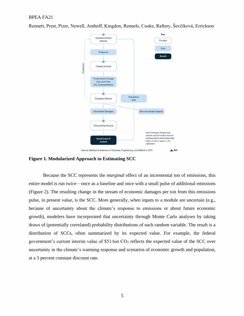
The NASEM report recommended creating an integrated framework comprising four

components (“modules”) underlying the SCC calculation:

• socioeconomics: probabilistic projections of population, gross domestic product (GDP),

and emissions over multiple centuries;

• climate: an improved model of Earth’s climate system and climate change;

• damages: the economic consequences of climate change, based on recent studies; and

• discounting: aggregated present-value marginal damages and stochastic discount factors

that correctly reflect the uncertain socioeconomic drivers (above).

Figure 1 shows how the modules fit together, including how socioeconomics affect

emissions trajectories, which are input into the climate model to project future temperatures.

These temperatures are converted into a stream of future economic losses in the damages model

(also influenced by socioeconomic trajectories), which are then discounted to a present value in

the discounting module.

BPEA FA21


5

Figure 1. Modularized Approach to Estimating SCC

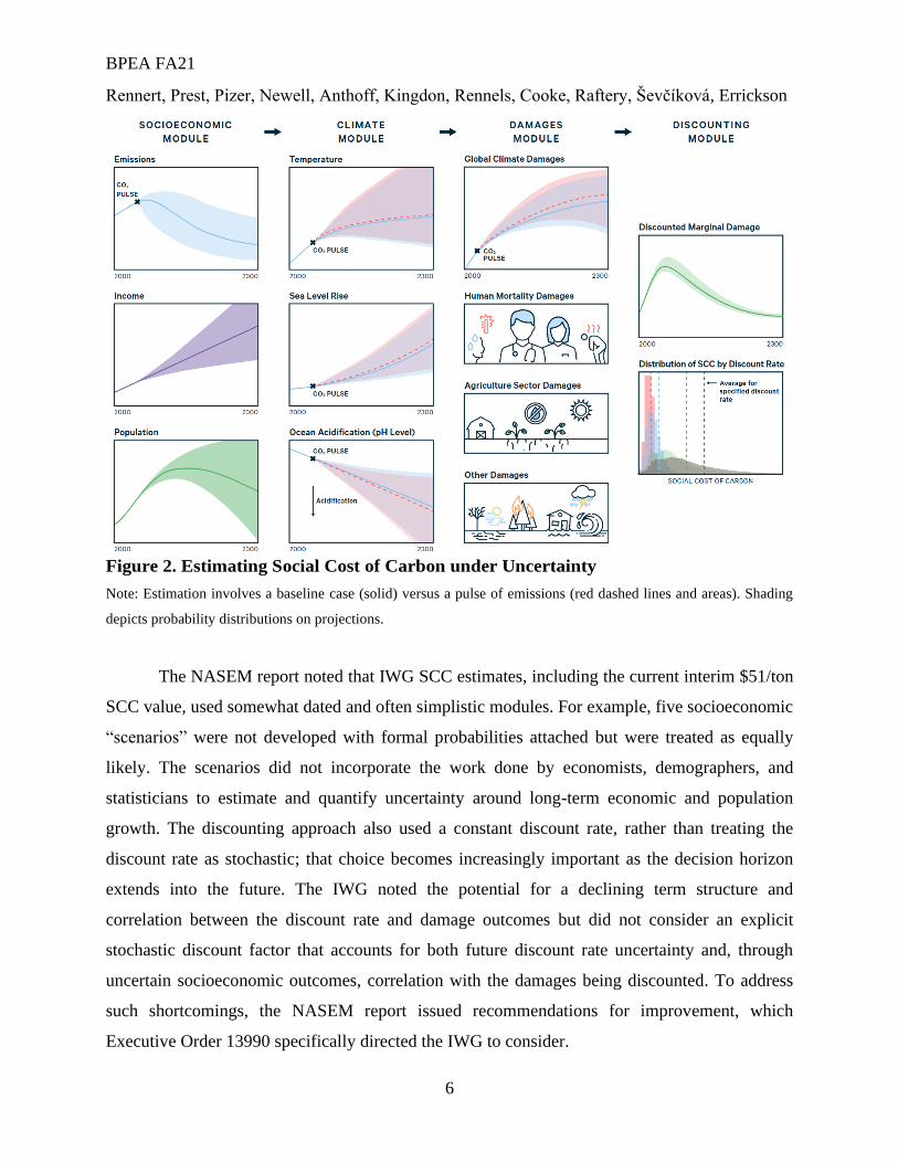
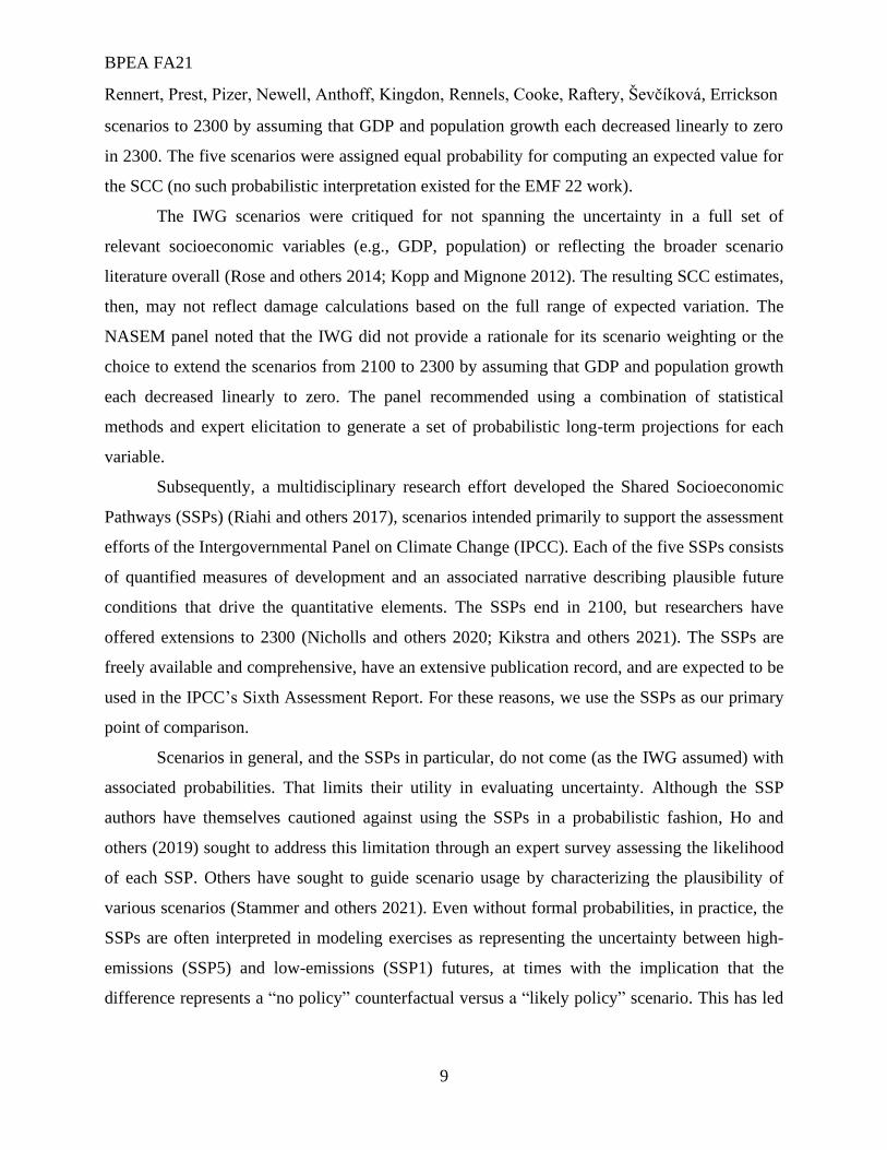
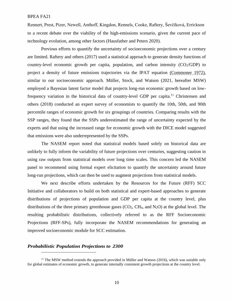
Because the SCC represents the marginal effect of an incremental ton of emissions, this

entire model is run twice—once as a baseline and once with a small pulse of additional emissions

(Figure 2). The resulting change in the stream of economic damages per ton from this emissions

pulse, in present value, is the SCC. More generally, when inputs to a module are uncertain (e.g.,

because of uncertainty about the climate’s response to emissions or about future economic

growth), modelers have incorporated that uncertainty through Monte Carlo analyses by taking

draws of (potentially correlated) probability distributions of each random variable. The result is a

distribution of SCCs, often summarized by its expected value. For example, the federal

government’s current interim value of $51/ton CO2 reflects the expected value of the SCC over

uncertainty in the climate’s warming response and scenarios of economic growth and population,

at a 3 percent constant discount rate.

BPEA FA21


6

Figure 2. Estimating Social Cost of Carbon under Uncertainty

Note: Estimation involves a baseline case (solid) versus a pulse of emissions (red dashed lines and areas). Shading

depicts probability distributions on projections.

The NASEM report noted that IWG SCC estimates, including the current interim $51/ton

SCC value, used somewhat dated and often simplistic modules. For example, five socioeconomic

“scenarios” were not developed with formal probabilities attached but were treated as equally

likely. The scenarios did not incorporate the work done by economists, demographers, and

statisticians to estimate and quantify uncertainty around long-term economic and population

growth. The discounting approach also used a constant discount rate, rather than treating the

discount rate as stochastic; that choice becomes increasingly important as the decision horizon

extends into the future. The IWG noted the potential for a declining term structure and

correlation between the discount rate and damage outcomes but did not consider an explicit

stochastic discount factor that accounts for both future discount rate uncertainty and, through

uncertain socioeconomic outcomes, correlation with the damages being discounted. To address

such shortcomings, the NASEM report issued recommendations for improvement, which

Executive Order 13990 specifically directed the IWG to consider.

BPEA FA21


7

This paper documents recent work that has improved the scientific basis for the modules

so that the IWG can update the SCC to reflect the best available science. Section II discusses the

improved socioeconomic module, with long-term probabilistic projections of population,

economic growth, and emissions. Section III illustrates how an incremental ton of emissions

translates into climate and economic effects (“damages”). Section IV discusses the crucial role of

the discount rate, given recent research on declining equilibrium interest rates, plus the

importance of using stochastic discount factors and the shadow price of capital for valuing

effects on investment. Section V then combines these elements into a simplified model of the

SCC, with associated uncertainty bounds for the socioeconomic, climate, damages, and

discounting components. Finally, section VI concludes and raises issues that await future

research.

II. Economic and Demographic Drivers of Climate Effects

Assessments of damages from climate change are influenced by projections of

population, economic growth, and emissions. Population growth can drive emissions and

increase or decrease total economic exposure to the health effects of climate change. Economic

growth similarly affects both the level of expected emissions and the resulting damages, which

are often estimated to scale with economic activity (Diaz and Moore 2017a). For example, the

monetization of mortality consequences typically depends on per capita income. Economic

growth projections can also influence the SCC through the discount rate if estimates are

calculated using Ramsey-like discounting, where the discount rate is a function of the rate of

economic growth: higher (lower) growth scenarios will yield a higher (lower) discount rate.

Finally, projections of global emissions determine the background state of the climate system

against which damages from an additional pulse of emissions are measured.

Estimates of the SCC are highly sensitive to socioeconomic and physical projections

(Rose and others 2017), but revised estimates have been based primarily on changes in

socioeconomic projections, not on improved understanding of the climate system (Nordhaus

2017b). Explicitly considering realistic, probabilistic socioeconomic projections is thus

important for improving the characterization of both the central tendency and the uncertainty in

the SCC.

BPEA FA21


8

A robust characterization of socioeconomic contributions to SCC estimates would ideally

incorporate probabilistic projections of population, economic growth, and emissions. The

particular requirements of SCC estimation, however, pose significant challenges for generating

such projections. One is the time horizon: given the long-lived nature of greenhouse gases in the

atmosphere, the SCC needs to account for discounted damages 200 to 300 years into the future

(NASEM 2017). Yet nearly all projections end at year 2100 and are often scenario-based rather

than probabilistic. New probabilistic projections that extend well into the future are required.

Another challenge is that although climate change can be projected from emissions

scenarios consistent with globally aggregated projections of economic activity and population

growth, the resulting climate damages are most appropriately estimated at a regional (or even

local) scale. Thus they require geographically disaggregated estimates of GDP and population.

A third challenge is that the future path of emissions likely depends on uncertain

improvements in technology and on the scale and success of policy interventions outside the

range of the historical record. That is, whereas historical data may be a reasonable guide to

forecast population and economic activity, the same is not true for emissions. The SCC should be

measured against our best estimate of future emissions, inclusive of future mitigation policies

except the one under analysis.

The fourth issue is the interrelated nature of these variables: the projections for each

variable must be consistent with one another. For example, emissions intensity might be lower

with higher economic growth (and its associated wealth and technological improvements).

Past Approaches to Socioeconomic Projections

In lieu of using fully probabilistic socioeconomic projections, researchers have typically

turned to socioeconomic scenarios, which can provide consistency across analyses and still

incorporate specific narratives. The IWG adopted a scenario approach in its initial estimates

(IWG SCC 2010), and these same scenarios support the interim estimates put forward by the

Biden administration in January 2021 (IWG SCC 2021). The IWG used five socioeconomic

scenarios drawn from the Energy Modeling Forum (EMF) 22 (Clarke and Weyant 2009)

modeling exercise, selected to roughly span the range of emissions outcomes in the full set of

EMF 22 scenarios and thus represent uncertainty across potential socioeconomic projections.

Only one of the scenarios represented future climate policy. The IWG extended the five

BPEA FA21


9

scenarios to 2300 by assuming that GDP and population growth each decreased linearly to zero

in 2300. The five scenarios were assigned equal probability for computing an expected value for

the SCC (no such probabilistic interpretation existed for the EMF 22 work).

The IWG scenarios were critiqued for not spanning the uncertainty in a full set of

relevant socioeconomic variables (e.g., GDP, population) or reflecting the broader scenario

literature overall (Rose and others 2014; Kopp and Mignone 2012). The resulting SCC estimates,

then, may not reflect damage calculations based on the full range of expected variation. The

NASEM panel noted that the IWG did not provide a rationale for its scenario weighting or the

choice to extend the scenarios from 2100 to 2300 by assuming that GDP and population growth

each decreased linearly to zero. The panel recommended using a combination of statistical

methods and expert elicitation to generate a set of probabilistic long-term projections for each

variable.

Subsequently, a multidisciplinary research effort developed the Shared Socioeconomic

Pathways (SSPs) (Riahi and others 2017), scenarios intended primarily to support the assessment

efforts of the Intergovernmental Panel on Climate Change (IPCC). Each of the five SSPs consists

of quantified measures of development and an associated narrative describing plausible future

conditions that drive the quantitative elements. The SSPs end in 2100, but researchers have

offered extensions to 2300 (Nicholls and others 2020; Kikstra and others 2021). The SSPs are

freely available and comprehensive, have an extensive publication record, and are expected to be

used in the IPCC’s Sixth Assessment Report. For these reasons, we use the SSPs as our primary

point of comparison.

Scenarios in general, and the SSPs in particular, do not come (as the IWG assumed) with

associated probabilities. That limits their utility in evaluating uncertainty. Although the SSP

authors have themselves cautioned against using the SSPs in a probabilistic fashion, Ho and

others (2019) sought to address this limitation through an expert survey assessing the likelihood

of each SSP. Others have sought to guide scenario usage by characterizing the plausibility of

various scenarios (Stammer and others 2021). Even without formal probabilities, in practice, the

SSPs are often interpreted in modeling exercises as representing the uncertainty between high-

emissions (SSP5) and low-emissions (SSP1) futures, at times with the implication that the

difference represents a “no policy” counterfactual versus a “likely policy” scenario. This has led

BPEA FA21


10

to a recent debate over the viability of the high-emissions scenario, given the current pace of

technology evolution, among other factors (Hausfather and Peters 2020).

Previous efforts to quantify the uncertainty of socioeconomic projections over a century

are limited. Raftery and others (2017) used a statistical approach to generate density functions of

country-level economic growth per capita, population, and carbon intensity (CO2/GDP) to

project a density of future emissions trajectories via the IPAT equation (Commoner 1972),

similar to our socioeconomic approach. Müller, Stock, and Watson (2021, hereafter MSW)

employed a Bayesian latent factor model that projects long-run economic growth based on low-

frequency variation in the historical data of country-level GDP per capita.11 Christensen and

others (2018) conducted an expert survey of economists to quantify the 10th, 50th, and 90th

percentile ranges of economic growth for six groupings of countries. Comparing results with the

SSP ranges, they found that the SSPs underestimated the range of uncertainty expected by the

experts and that using the increased range for economic growth with the DICE model suggested

that emissions were also underrepresented by the SSPs.

The NASEM report noted that statistical models based solely on historical data are

unlikely to fully inform the variability of future projections over centuries, suggesting caution in

using raw outputs from statistical models over long time scales. This concern led the NASEM

panel to recommend using formal expert elicitation to quantify the uncertainty around future

long-run projections, which can then be used to augment projections from statistical models.

We next describe efforts undertaken by the Resources for the Future (RFF) SCC

Initiative and collaborators to build on both statistical and expert-based approaches to generate

distributions of projections of population and GDP per capita at the country level, plus

distributions of the three primary greenhouse gases (CO2, CH4, and N2O) at the global level. The

resulting probabilistic distributions, collectively referred to as the RFF Socioeconomic

Projections (RFF-SPs), fully incorporate the NASEM recommendations for generating an

improved socioeconomic module for SCC estimation.

Probabilistic Population Projections to 2300

11 The MSW method extends the approach provided in Müller and Watson (2016), which was suitable only

for global estimates of economic growth, to generate internally consistent growth projections at the country level.

BPEA FA21


11

Methods. To develop probabilistic, country-level population projections through 2300,

we start with the fully probabilistic statistical approach that has been used since 2015 by the

United Nations (UN) for its official population forecasts to 2100. We then extend the

statistical model to 2300, incorporating feedback and improvements suggested by a panel of

nine leading demographic experts that we convened to review preliminary results. This

work is detailed in Raftery and Ševčíková (2022, forthcoming).

The UN uses a probabilistic method built on the standard deterministic cohort-

component method of population forecasting (Preston, Heuveline, and Guillot 2001). This

method projects forward the three components of population change: fertility, mortality and

migration, broken down by age and sex. The probabilistic method builds Bayesian

hierarchical models for each of the three components and projects them forward

probabilistically using a Markov chain Monte Carlo (MCMC) method, which produces a

large number (typically 1,000-2,000) of trajectories of future numbers of births, deaths, and

migration events in each country by age and sex. Each trajectory of fertility, mortality and

migration is then combined to give a trajectory of future population by age and sex in each

country. These 1,000-2,000 trajectories of population numbers in turn approximate a

probability distribution for any population quantity of interest (Raftery and others 2012;

Raftery, Alkema, and Gerland 2014; Gerland and others 2014).

Fertility is projected by focusing on each country’s Total Fertility Rate (TFR), which

is the expected number of children a woman would have in a given period if she survived

the reproductive period (typically to age 50) and at each age experienced the age-specific

fertility rates of that period. The UN models the evolution of fertility in all countries using a

Bayesian hierarchical model that divides it into three phases depending on where it lies in

the fertility transition from high to low fertility (pre-transition, transition, post-transition). It

then fits a time series model to each phase, accounting for spatial correlation between

countries (Alkema and others 2011; Raftery, Alkema, and Gerland 2014; Fosdick and

Raftery 2014; United Nations 2019; Liu and Raftery 2020).12 Mortality is similarly

12 The TFR has evolved in a similar way in all countries. Typically, in pre-industrial times, the TFR for a typical

country was high (in the range 4-8 children per woman). Then, usually after the onset of industrialization, it started

to decrease. After a bumpy decline lasting several decades to a century, the TFR flattened out at a level below the

BPEA FA21


12

projected by focusing on life expectancy at birth.13 This is projected by another Bayesian

hierarchical model for all countries for both sexes (Raftery and others 2013; Raftery, Lalic,

and Gerland 2014). The UN has traditionally projected net international migration for each

country deterministically by assuming that it would continue in the future at the same rate as

currently (United Nations 2019).

We extended this UN method, designed for projections to 2100, out to 2300 and

preliminary results were reviewed by a panel of nine expert demographers that we

convened. While broadly supportive, the panelists were in agreement that the resulting

uncertainty bounds for TFR in 2300 were too narrow, and that in particular the lower bound

of the 95% prediction interval for world TFR in 2300 (1.66) was too high. A lower bound of

1.2 children per woman for the world TFR in 2300 was suggested as a more plausible lower

bound. We incorporated this recommendation by adding a worldwide random walk

component to the TFR model.

Experts on the panel also suggested that international migration should be projected

probabilistically, in line with the general approach, rather than deterministically as done by

the UN. We implemented this by projecting net international migration using a Bayesian

hierarchical model (Azose and Raftery 2015; Azose, Ševčíková, and Raftery 2016). We

additionally implemented the final panel recommendation, to impose constraints on

population density to prevent unrealistically high or low population numbers in some age

groups in some countries.

Results. The resulting population projections for 2300 for the world as a whole and

for the continents, are shown in Figure 3. They show that total world population is likely to

continue to increase for the rest of the 21st century, albeit at a decreasing rate, to level off in

the 22nd century, and to decline slightly in the 23rd century. Uncertainty for 2300 is

replacement rate of about 2.1 children per woman. This decline is called the fertility transition. After the end of the

fertility transition, the TFR has fluctuated without a clear trend, mostly staying below the replacement rate. For

example, in the US, the TFR was around 7 children per woman in 1800, and then declined, reaching 1.74 in 1976,

and thereafter fluctuating up and down; it is now 1.64, close to the level it was at in 1976 (Raftery 2021).

13 The general trend since 1840 has been that life expectancy has increased steadily (Oeppen and

Vaupel 2002), with slower increases for countries with the lowest and highest life expectancy, and the fastest

increases for countries in the middle.

BPEA FA21


13

considerable, appropriately, reflecting the very long forecast time horizon, with a median

forecast of 7.5 billion, but a 95% interval from 2.3 to 25.8 billion. The results agree closely

with the UN forecasts for the period to 2100 (United Nations 2019).

Figure 3 also shows the results for each major continental region. They show that the

populations of Asia, Europe and Latin America are likely to peak well before the end of this

century and then decline substantially. The populations of Africa and Northern America are

also likely to peak and then decline, but much later, in the 22nd century. In the case of Africa

this is due to population momentum (with a high fraction of the population currently in

reproductive ages) and current high fertility. In the case of Northern America it is due to a

combination of modest population momentum, fertility that is closer to replacement level

than in other continents, and immigration. Uncertainty for each region in 2300 is high.

In comparison to the population projections from the SSPs, our population projections are

centered around a peak of slightly over 10 billion people globally reached late this century, lying

closest to SSP2, although SSP2 levels off at a higher level than our median projection after 2200.

Through 2300, the 90% confidence distribution around our median is narrower than the range

indicated by the SSPs, and considerably narrower through 2200. SSP1 and SSP5 lie below the

5th percentile of our distribution through almost the entire time horizon to 2300. SSP3 features a

very aggressive population projection in the top tail of the distribution, at about the 99th

percentile in 2300. In sum, none of the SSPs has a central tendency for population in line with

our fully probabilistic projections, and the range of population given by SSP1-SSP5 is wide

relative to ours.

We are aware of only three other detailed efforts to project world population to 2300,

all of them deterministic, in contrast with our probabilistic method described here. One was

carried out by United Nations (2004) and was deterministic, but containing several scenarios.

The range of these projections for 2300 from the different scenarios went from 2.3 to 36.4

billion, compared with our 98% prediction interval of 1.7 to 33.9 billion. Although using

BPEA FA21


14

different methodologies and carried out over 15 years apart, the two sets of projections give

results that are compatible with one another, perhaps to a surprising extent.14

Another such exercise was carried out by Vallin & Caselli (1997), also deterministic

with three scenarios corresponding to different long-term trajectories of world TFR. Two of

the scenarios led to world population stabilizing at around 9 billion, while the other resulted

in 4.3 billion people in 2300. All three of these scenarios give world population in 2300 well

within our 80% interval, though with a range that is much narrower than either ours or that

of United Nations (2004). Gietel-Basten and others ( 2013) also performed a projection

exercise to 2300, with a very wide range of scenarios for long-term world TFR. They

obtained projections of global population yielding anything from zero to 86 billion in

2300.15

Figure 3. Probabilistic Population Projections for World and Major Regions, to 2300

Notes. Data prior to 2020 are from the UN’s World Population Prospects 2019 (UN 2019). The predictive

medians are shown as solid curves; the shaded areas show the 90% and 98% predictive intervals. The world

population projections from the extended SSPs are shown for comparison.

Probabilistic Economic Growth Projections to 2300 and Economic Growth Survey

14 The very high upper bound for the UN (2004) projections is likely an artifact due to the perfect

correlation implied by the deterministic scenarios and the aggregation of such results. 15 As in the UN (2004) projections, these very extreme outcomes are likely in part due to the perfect

correlation between countries implied by the deterministic scenarios and the aggregation of such results.

BPEA FA21


15

Methods. The probabilistic projections of economic growth often used in analyses by

governments and the private sector have not incorporated the time scale of centuries, as is needed

to support SCC estimates and other economic analyses of climate change. MSW (2019) took a

significant step forward by providing probabilistic econometric projections over long periods.

The MSW methodology involves a multifactor Bayesian dynamic model in which each country’s

GDP per capita is based on a global frontier of developed economies (countries in the

Organisation for Economic Co-operation and Development, OECD) and country-specific

deviations from that frontier. Correlations between countries are also captured in a hierarchical

structure that models countries in “covariance clubs,” in which country-level deviations from the

frontier vary together. The hierarchical structure also permits pooling information across

countries, an approach that tightens prediction intervals. This model is then estimated on data for

113 countries over 118 years (1900 to 2017). The model yields 2,000 sets of trajectories of

country-level GDP per capita from 2018 to 2300. Each can be considered an equally likely

uncertain future. Each is characterized by a path for the global factor and 113 country-specific

deviations from that pathway. The results are described more fully below; for more information

about the model, see MSW (2019).

As noted earlier, however, NASEM (2017) recommended augmenting statistical models

with formal expert elicitation to quantify uncertainty, especially for long-term projections. But

surveying experts on long-term uncertainty of economic growth at the country level is

impractical because of time constraints and the difficulty of accounting for intercountry

correlations. Consequently, our study was designed to work in tandem with an econometric

model that provides country-level projections and represents the intercountry dynamics. Our

Economic Growth Survey (EGS) focused on quantifying uncertainty for a representative frontier

of economic growth in the OECD countries. The results informed econometric projections based

on the MSW model of an evolving frontier (also based on the OECD), in turn providing country-

level, long-run probabilistic projections.

The methodology we applied is the “classical model” (Cooke 1991, 2013) of structured

expert judgment, analogous to classical hypothesis testing. In essence, the experts are treated as

statistical hypotheses: they are scored on their ability to assess uncertainty based on their

responses to calibration questions whose true values are known to us but unknown to the experts.

This scoring allows us to weight the experts’ judgments, and the scores of combinations of

BPEA FA21


16

experts serve to gauge and validate the combination that is adopted. The ability to performance-

weight experts’ combined judgments has generally been shown to provide the advantages of

narrower overall uncertainty distributions with greater statistical accuracy and improved

performance both in and out of sample (Colson and Cooke 2017, 2018; Cooke and others 2021).

Ten experts, selected for their expertise in macroeconomics and economic growth and

recommended by their peers, were elicited individually by videoconference in roughly two-hour

interviews in 2019–2020. They received an honorarium where appropriate. The full elicitation

protocol is available in the online appendix; the general process was as follows. First, experts

quantified their uncertainty for several initial questions, after which answers were provided for

self-assessment; this step was intended to familiarize them with the process and alert them to

potential biases. The experts then provided a median and 90 percent confidence range for 11

calibration questions for which the true values were known to us.

Experts next provided their 1st, 5th, 50th, 95th, and 99th quantiles for the variables of

interest: levels of OECD GDP per capita for 2050, 2100, 2200, and 2300. For experts more

comfortable working in growth rates (rather than levels), we provided a spreadsheet tool that

translated average growth rates into GDP per capita levels. Experts were informed that their

combined quantiles of GDP levels would be combined with country-level econometric

projections, as described below, but they were not shown the results. Experts were given

historical data on economic growth to provide a consistent baseline of information across the

panel, and they were permitted to consult outside sources if desired. Experts provided additional

rationale for their quantiles verbally throughout the elicitation and concluded the survey by

formally identifying the primary factors driving their low and high future growth scenarios.

Given that the projections were being used as an input to the estimation of climate change

damages, which would reduce economic activity below the projected level, experts were

specifically asked to provide quantiles of economic growth absent the effects of further climate

change as well as absent further policy efforts to reduce emissions. Two of the 10 experts

provided a pair of modified base quantiles to reflect the absence of effects from climate damages

and climate policy, but in general the proposed modifications to their original distributions were

minor. Moreover, several experts noted that although climate change was a primary driver of

their low growth projections, the complexity of the uncertainties represented in their base

BPEA FA21


17

quantiles precluded their systematic removal, and they deemed their base quantiles appropriate

for assessing uncertainty in analyses intended to include the effects of climate change.

The results of the expert elicitations were combined by first fitting each expert’s five

quantiles for each year, in log GDP per capita, with a Johnson SU distribution (Johnson 1949) to

generate a continuous cumulative distribution function (CDF) specific to each expert. We next

combined the CDFs in two ways: averaging across the set of expert CDFs with equal weight, and

performance-weighting the experts according to their performance on the calibration questions.

This process yielded a pair of final combined elicited values of OECD GDP per capita for each

elicited year and quantile.16

Results of Economic Growth Survey. On the calibration questions (see online appendix),

the experts demonstrated an overall high level of statistical accuracy compared with other

structured expert judgment studies and results that are robust against expert loss. As shown by

their individual quantiles (Figure 4) and as expressed in comments during the videoconferences,

most participants’ median forecast was that long-term growth would be lower than the growth

rate of the past 100 years. The responses show considerable diversity in their characterization of

uncertainty around the median, however, with some of the widest ranges being driven by their

explicit inclusion of events that are not present or fully realized in the historical record of

economic growth on which statistical growth projections are based.17 When asked to identify the

primary drivers of the low-growth quantiles, the experts most commonly responded climate

change, followed by world conflict, natural catastrophes, and global health crises. Rapid

advancement of technology was cited most often as the primary driver of high growth, followed

by regional cooperation and advances in medical science. Many experts expected that technology

breakthroughs in clean energy would dramatically lower global emissions. Implicit in this

narrative is a negative correlation between economic growth and carbon dioxide emissions.

As shown in Figure 4, both the performance-weighted and the equal-weighted

combinations of the experts’ distributions yield narrower ranges as well as lower medians than

16 See online appendix for further detail. 17 The quantiles from one expert included global civilization-ending events that were outside the scope of

the survey and incompatible with assumptions for US federal policy analysis; they unreasonably distorted the

combined distributions toward extreme values. Quantiles from this expert were excluded in the final survey.

BPEA FA21


18

do the statistical trajectories for all four years (2050, 2100, 2200, and 2300). The median of the

equal-weighted combination is consistently higher than that based on performance weighting, but

the difference shrinks throughout the period until the medians nearly converge in 2300. Overall,

the experts viewed sustained long-term growth rates above 4 percent or even slightly below 0

percent as highly unlikely but not impossible.

Results of econometric growth projections augmented with expert judgment. We used the

EGS results to modify econometric projections of GDP per capita based on the MSW (2019)

methodology and generate density functions of internally consistent projections of economic

growth at the country level. As indicated in MSW (2019), economic growth 100 to 300 years

into the future is highly uncertain, well beyond that captured in typical scenario projections (see

Figure 5 below).

Figure 4. Distributions of Future Average GDP Growth Rates for OECD from Experts

and Econometric (MSW) Sources

Note. For each bar, the circle shows the median and the lines show the 1st, 5th, 95th, and 99th percentiles of

the relevant distribution.

The tails of the MSW distribution are quite wide, leading to some implausibly small or

implausibly high long-term average growth rates in the extreme tails (e.g., below the 1st

BPEA FA21


19

percentile or above the 99th percentile). These extreme tails correspond to extremes of persistent

economic growth beyond what has been observed historically over long periods (e.g., below –1

percent or above +5 percent annually on average through 2300). Specifically, according to the

Maddison Project dataset (one of two datasets used by MSW),18 which includes country-level

GDP per capita data as far back as 1500 for some countries, no country has experienced such

extreme growth for such long periods.19 In the MSW model, those extreme tail simulated

outcomes are driven by the structure of the Bayesian model with its embedded distributional

assumptions, rather than by the historical data used to estimate the model.

Further, the 1st and 99th percentiles of the combined distribution of long-run growth rates

based on the EGS are –0.6 percent and +4.4 percent, indicating that long-run growth rates are

unlikely to fall outside this range. For these reasons, and in consultation with James Stock (an

MSW coauthor), we omit some projections in the extreme tails of the MSW distribution that are

outside the range of historical experience and also outside the long-run range implied by the EGS

(see online appendix for our approach). Hereafter, we refer to this censored MSW version as the

“MSW projections,” while noting that it differs slightly in the extreme tails.

The EGS provides quantiles of economic growth for the OECD for four discrete years.

To maintain the rich country-level information of the econometric model while incorporating the

information from the experts, we reweight the probability of occurrence of each of the 2,000

MSW draws to satisfy the experts’ combined distribution over the long run. The underlying

projections from MSW remain unchanged, but the likelihood of drawing a given trajectory is

modified such that the quantiles of OECD growth reflect the distribution produced by the EGS.

We accomplish this reweighting in two steps. First, we generate a set of target quantiles

for the years 2030, 2050, 2100, 2200, and 2300 by calculating weighted averages of the

combined expert quantiles and the raw MSW quantiles. The NASEM report recommended

giving expert judgment increasing weight for longer horizons, so the near-term weighting is

governed more by historical evidence and that of the long-term future more by the experts. For

18 Available at https://clio-infra.eu/Indicators/GDPperCapita.html. 19 For example, no country in Maddison Project data has observed 100-year growth rates below –1 percent

or above +3 percent.

https://clio-infra.eu/Indicators/GDPperCapita.html

BPEA FA21


20

this reason, we increase the weight of the EGS quantiles versus the MSW quantiles linearly over

time from 0 percent in 2030 to 100 percent in 2200 and thereafter.

We then use iterative proportional fitting (Csiszar 1975) to impose the target quantiles for

OECD growth on the 2,000 trajectories from MSW for each of the four benchmark years. For

each range of values between each elicited quantile, this algorithm reassigns probabilities to each

trajectory whose value falls within that range by minimizing a penalty for nonequal weights,

subject to matching the target quantiles. Because there are four years for which we have a

combined expert distribution to satisfy, the algorithm iterates between each year until all years’

distributions are satisfied. Figure 5 compares the resulting distributions from MSW with those

reweighted according to the EGS.

BPEA FA21


21

Figure 5. Average Projected Growth Rates of GDP per Capita in OECD Countries

Notes. Adapted from MSW (2019) and an EGS performance-weighted average of those data. Shaded areas and

dashed/dotted lines represent 5th to 95th (darker, dashed) and 1st to 99th (lighter, dotted) percentile ranges.

BPEA FA21


22

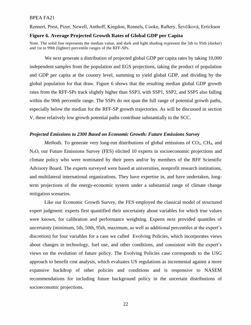
Figure 6. Average Projected Growth Rates of Global GDP per Capita

Note. The solid line represents the median value, and dark and light shading represent the 5th to 95th (darker)

and 1st to 99th (lighter) percentile ranges of the RFF-SPs.

We next generate a distribution of projected global GDP per capita rates by taking 10,000

independent samples from the population and EGS projections, taking the product of population

and GDP per capita at the country level, summing to yield global GDP, and dividing by the

global population for that draw. Figure 6 shows that the resulting median global GDP growth

rates from the RFF-SPs track slightly higher than SSP3, with SSP1, SSP2, and SSP5 also falling

within the 90th percentile range. The SSPs do not span the full range of potential growth paths,

especially below the median for the RFF-SP growth trajectories. As will be discussed in section

V, these relatively low growth potential paths contribute substantially to the SCC.

Projected Emissions to 2300 Based on Economic Growth: Future Emissions Survey

Methods. To generate very long-run distributions of global emissions of CO2, CH4, and

N2O, our Future Emissions Survey (FES) elicited 10 experts in socioeconomic projections and

climate policy who were nominated by their peers and/or by members of the RFF Scientific

Advisory Board. The experts surveyed were based at universities, nonprofit research institutions,

and multilateral international organizations. They have expertise in, and have undertaken, long-

term projections of the energy-economic system under a substantial range of climate change

mitigation scenarios.

Like our Economic Growth Survey, the FES employed the classical model of structured

expert judgment: experts first quantified their uncertainty about variables for which true values

were known, for calibration and performance weighting. Experts next provided quantiles of

uncertainty (minimum, 5th, 50th, 95th, maximum, as well as additional percentiles at the expert’s

discretion) for four variables for a case we called Evolving Policies, which incorporates views

about changes in technology, fuel use, and other conditions, and consistent with the expert’s

views on the evolution of future policy. The Evolving Policies case corresponds to the USG

approach to benefit cost analysis, which evaluates US regulations as incremental against a more

expansive backdrop of other policies and conditions and is responsive to NASEM

recommendations for including future background policy in the uncertain distributions of

socioeconomic projections.

BPEA FA21


23

Experts provided quantiles of uncertainty for (1) fossil fuel and process-related CO2

emissions; (2) changes in natural CO2 stocks and negative-emissions technologies; (3) CH4; and

(4) N2O, for five benchmark years: 2050, 2100, 2150, 2200, and 2300. For category 1, they were

also asked to indicate the sensitivity of emissions to five GDP per capita trajectories.20

For each expert we generate a set of cumulative distribution functions (CDFs), one for

each benchmark year, emissions source, and economic growth trajectory, by piecewise linear

interpolation between the quantiles provided. Then, as in the EGS, we generate a corresponding

set of combined equal-weight CDFs by averaging the CDFs in equal measure, and a set of

performance-weighted CDFs by averaging in accordance with the experts’ relative performance

on the calibration questions. Quantile values from the combined CDFs were linearly interpolated

in time between each of the benchmark years to yield a distribution of piecewise linear,

nonoverlapping trajectories for each emissions source and sink.

Based on the FES, we developed a distribution of emissions scenarios to pair, 1-1, with our

economic growth scenarios. First, we sampled from one of 10,000 economic growth trajectories,

described above. Second, we sampled a value (q) on the continuous interval [0,1] to determine

the percentile of the expert’s emissions trajectory to evaluate. Third, at five-year intervals from

2025 to 2300 we generated an interpolated value of the qth percentile of emissions based on the

realized GDP level corresponding to that GDP trajectory in that year, and the qth percentile of

the experts’ emissions distributions for the bounding GDP values elicited. Net emissions of CO2

were generated by sampling independent q values for direct emissions (category 1) and natural

carbon stocks and negative emissions technologies (category 2) and summing the resulting

trajectories, thereby including the possibility of net negative emissions.21

20 See online appendix for a more detailed discussion of the survey methodology and the full elicitation

protocol. 21 The experts received real-time feedback about the implications of their prescribed distributions for future

outcomes. After each had provided a full set of quantiles, we followed the same sampling process described above

to generate distributions of emissions trajectories, except that the emissions distributions were based on input

provided by only that expert rather than the full set of experts, and that for expediency we presented results based on

100 to 1,000 samples at the discretion of the expert. Experts were shown their full distributions of emissions

trajectories, the economic growth paths sampled, population, emissions intensity, and the resulting climate outcomes

from the FaIR 2.0 climate model (described in section III) for their verification. They were permitted to modify their

quantiles after seeing their distributions and resulting climate outputs, but in general they found the results to be in

agreement with the intent of their quantiles and consistent with their supporting rationale.

BPEA FA21


24

Results of the Future Emissions Survey. Experts’ performance on the calibration

questions was high, as measured by statistical accuracy, informativeness, and robustness of

results (see online appendix). Experts described their rationale and the conditions supporting

their distributions of emissions, often citing the same factors. For direct CO2 emissions (category

1), experts viewed low economic growth as likely to reduce emissions overall but also lead to

reduced global ambition in climate policy and slower progress to decarbonization. For median

economic growth conditions, experts generally viewed policy and technology evolution as the

primary driver of their emissions distributions, often offering a median estimate indicating

reductions from current levels but with a wide range of uncertainty. Several experts said high

economic growth would increase emissions through at least 2050, most likely followed by rapid

and complete decarbonization, but with a small chance of substantial continued increases in

emissions. In general, the distributions were inconsistent with keeping global temperature

increases below 1.5 degrees C, even when considering the potential for negative emissions. 22

Though their rationales were often similar, experts’ interpretation of those narratives, as

shown in their quantiles of emissions, differed substantially (Figure 7). For example, for the

median growth trajectory to 2050, the median emissions ranged from 15 to 45 Gt CO2, a span

encompassing a decrease of more than 50 percent to an increase of more than 30 percent from

today’s levels. Experts often provided highly skewed distributions, with significant chances that

direct CO2 emissions (category 1) would be exactly or near zero while allowing for much higher

emissions in the middle and upper quantiles of their distribution.23

22 See online appendix for a more detailed summary of the rationales of the experts, including discussion of

emissions from the other categories. 23 See online appendix for results for additional years and gases.

BPEA FA21


25

Figure 7. Cumulative Distribution Functions (CDFs) of Annual CO2 Emissions

Panel (A): Individual Expert and Combined CDFs for 2050

Panel (B): Combined CDFs of Expert Projections for 2050 to 2300

The experts’ narratives show an evolution of the combined distributions (Figure 8). Over

time, emissions distributions for all growth trajectories exhibit a shift, particularly evident for the

median and high-growth trajectories, with median emissions approaching zero in and after 2150.

Emissions distributions for the lower-growth trajectory show a decreased range of emissions

overall compared with the higher-growth trajectories, but the temporal trend toward lower

emissions is not as strong. Higher-growth trajectories show relatively greater probabilities of

increased emissions in the near term, followed by greater chances of full decarbonization in the

next century, while also allowing for the possibility of much higher emissions over the long

term. (For the other categories of emissions sources and sinks, see online appendix).

Resulting global greenhouse gas emissions projections. Figure 8 shows the resulting

distribution of projected net CO2 emissions based on the FES. The median emissions trajectory is

a roughly 50 percent decrease from today’s levels by 2100, followed by slowly decreasing levels

that approach but do not reach net zero. The median of our CO2 emissions and concentrations

BPEA FA21


26

paths is similar to SSP2, and the 98 percent confidence interval spans a range similar to that of

SSP1 through SSP3, at least through 2140.24 The magnitude of CO2 emissions associated with

SSP5, however, is considerably higher than the upper end (99th percentile) of our distribution

through the middle of the next century, consistent with the findings of Raftery and others (2017)

and Liu and Raftery (2021). Beyond the middle of the next century, all the SSP emissions

trajectories increasingly lie well within our distribution because their extension beyond 2100 is

constructed to achieve zero emissions by 2250. This is a weakness of the SSPs as a basis for

SCC estimation, even if a subset of the SSPs spans a “reasonable range” during this century.

For CH4 (Figure OA-9), the emissions and concentrations distribution resulting from the

FES is centered between SSP2 and SSP5 and spans a range similar to that of SSP1–SSP5, at least

through 2100. After that point, as with CO2, the emissions range spanned by the SSPs narrows,

whereas the FES CH4 emissions maintain a relatively wide distribution, similar to that in 2100.

For N2O (Figure OA-10), the centers of the FES emissions and concentrations paths is similar to

that of SSP5, and the full distribution from the FES spans a range wider than all the SSPs.

In sum, no single SSP is centered similarly to the FES median emissions paths across all

three major greenhouse gases. The full range of emissions represented by the SSPs is higher than

for the FES for CO2 through 2140, by construction narrows to zero for CO2 after that point, and

is narrower than the FES results for CH4 and N2O after 2100.

24 For comparison of emissions consistent with the SSPs beyond 2100, we adopt the commonly used

extensions provided by the Reduced Complexity Model Intercomparison Project (Nicholls and others 2020).

BPEA FA21


27

Figure 8. Net Annual Emissions of CO2 from RFF-SPs and SSPs

Notes. Lines represent median values, and dark and light shading represent the 5th to 95th (darker) and 1st to

99th (lighter) percentile ranges of the RFF-SPs.

III. From Emissions to Monetized Climate Damages

Climate system methods. The second step in estimating the SCC is using a climate

model to calculate changes in the climate system corresponding to changes in GHG emissions.

Climate models vary in their representation of the underlying physics, in their spatial and

temporal resolution, and in their computational requirements. Earth system models, such as those

used for IPCC analyses, require supercomputers, but SCC calculations, typically generated from

tens to hundreds of thousands of samples to characterize their uncertainty, preclude use of full-

scale earth system models. SCC models are designed to emulate the response of full earth system

models across a subset of relevant climate outputs, such as globally averaged surface

temperature.

Previous SCC calculations from the federal government used the integrated assessment

models DICE, FUND, and PAGE, each of which employs its own reduced-form climate model.

These IAMs can deliver substantially different temperature increases for the same pulse of

emissions (Rose and others 2014), leading to inconsistency when results are averaged to

BPEA FA21


28

calculate the SCC. The NASEM report therefore recommended adopting a uniform climate

model that met certain criteria, including that it generate a distribution of outputs across key

climate metrics comparable to distributions of outputs from the full earth system models.

The Finite Amplitude Impulse Response (FaIR, Millar and others 2017) model was

highlighted in the NASEM report as a reduced-form model that met the criteria. To assess the

changes in global mean surface temperatures resulting from the RFF-SPs, we ran the latest

version, FaIR 2.0 (Leach and others 2021), using 10,000 draws from the emissions trajectories of

CO2, CH4, and N2O while also sampling across FaIR’s native uncertainty in climate variables.25

Resulting temperature change from RFF-SPs. Figure 9 shows the median temperature

trajectory associated with the RFF-SPs: increases reaching nearly 3 degrees C above the average

global temperature for 1850–1900 (the standard IPCC preindustrial benchmark) through 2100,

and continued increases through 2300. The low end of the distribution indicates a roughly 5

percent chance that the increase will remain below 2 degrees C through 2100. Our experts’

expectations for negative-emissions technologies lead to an increasing chance of drawing down

atmospheric CO2 to yield temperatures at current levels and below by the late 2100s.

The RFF-SP median temperature trajectory tracks closely with SSP2 through 2200,

thereafter continuing to increase slightly. SSP1 is largely consistent with the 5th percentile

results throughout the period. Temperatures resulting from SSP3 emissions are consistent with

the 95th percentile of the RFF-SPs through the middle of the next century, at which point

temperatures stop increasing, by construction. The median temperature from SSP5 is roughly

consistent with the 99th percentile of temperatures from the RFF-SPs through 2100, at which

point it begins to level off to meet the imposed requirement for net-zero emissions by 2250.

25 Trajectories for non-CO2, CH4, and N2O were drawn from SSP2.

BPEA FA21


29

Figure 9. Global Mean Surface Temperature Change from RFF-SPs and SSPs

Notes. Temperature change is relative to the standard 1850–1900 preindustrial average. Solid lines represent

median values. Dark and light shading represent the 5th to 95th (darker) and 1st to 99th (lighter) percentile

ranges based on the RFF-SPs. For clarity of presentation, uncertainty in the climate system is reflected in the

uncertainty range only for the RFF-SPs (and not the SSPs).

In this comparison, uncertainty in the climate system itself, as represented by the

uncertain distributions of climate parameters in the FaIR model, contributes significant

uncertainty to the range of projected temperatures. The temperature distributions for the RFF-

SPs include climate uncertainty from FaIR, but for clarity we omit climate system uncertainty in

presenting projected temperatures from the SSPs. For a sense of scale, the 90th percentile range

in temperatures from FaIR in 2300 for SSP5 is about –2.5 to +7 degrees C about the median.

Methods for climate damage estimation. The third step in estimating the SCC is

translating changes in the climate system, such as temperature, into total economic damages over

time. Damages can be calculated by estimating costs for various sectors (e.g., human health and

mortality, agriculture, energy usage, coastal flooding) and summing them, or by taking an

aggregate approach to estimate damages across the economy as a whole.

BPEA FA21


30

Recent advances in methodologies for damage estimation are not reflected in the IAMs

used by the federal government to calculate the SCC (NASEM 2017; Diaz and Moore 2017).

The NASEM report made recommendations on improving sectoral damage estimation, finding

sufficient peer-reviewed research to support updates on human health and mortality, agriculture,

coastal inundation, and energy demand. Since the report was issued, the literature addressing

specific sectors has grown.

Nevertheless, few studies meet the full requirements (e.g., global coverage with regional

detail, translation into economic damages) put forward by Diaz and Moore (2017b) or Raimi

(2021) to serve as the basis for an updated damage function for the SCC. For example, two

independent, comprehensive reviews (Bressler 2021; Raimi 2021) found just three suitable

studies (World Health Organization 2014; Gasparrini and others 2017; Carleton and others

2018). Our own further assessment of the damages literature found two candidates for

agricultural damages (Moore and others 2017; Calvin and others 2020), two for energy demand

(Clarke and others 2018; Ashwin and others 2021), and one for coastal damages (Diaz 2016).

Among the notable additions, the Climate Impact Lab (CIL) has developed a methodology

to generate empirically derived, hyper-localized damage functions accounting for adaptation.

The CIL in its research has been applying its methodology across a comprehensive set of sectors

including health, agriculture, labor, energy, conflict, coastal, and migration (Carleton and others

2018). Upon completion, this full set of sectors is intended to support fully empirically based

climate damage estimates.

Much of the new sectoral damages research identified here is currently under peer-review

for publication, and efforts to implement the existing peer-reviewed studies will similarly be

completed on a timeline that is compatible with the IWG process to update the SCC. As

described below, for the purposes of this paper we have deployed the aggregate global climate

damage function from the widely used DICE model (Nordhaus 2017b) to develop illustrative

SCC estimates, coupled with the RFF-SPs, the FaIR climate model, and the stochastic

discounting approach described in the next section.

BPEA FA21


31

IV. Discounting Approaches for the Social Cost of Greenhouse Gases

The long residence time of CO2 in the atmosphere implies that today’s emissions will

have consequences for centuries. This time horizon makes the discount rate a major factor for the

SCC. For example, the IWG’s 2021 interim SCC estimate is $51/ton with a 3 percent discount

rate (IWG SCC 2021) but would be about $121/ton at a 2 percent discount rate (RFF and

NYSERDA 2021). That 1 percentage point difference alone would more than double the SCC

and, by implication, greatly strengthen the economic rationale for substantial emissions

reductions.

The discount rates used in federal regulatory analysis are guided by Circular A-4, issued

by the Office of Management and Budget (OMB) in 2003, which endorses rates of 3 percent and

7 percent reflecting, respectively, consumption and investment rates of return. OMB guidance

also allows for additional sensitivity analysis in cases with intergenerational consequences, such

as climate change. However, this guidance runs counter to current economic thought and

evidence, for three reasons: (1) a constant deterministic discount rate becomes increasingly

problematic for long-horizon problems (Weitzman 1998); (2) benchmarks for the consumption

rate of interest (currently 3 percent) have declined substantially over the past two decades (CEA

2017; Bauer and Rudebusch 2020, 2021); and (3) the rationale for 7 percent—to address possible

policy effects on capital—is flawed in ways that are magnified for very long-term decisions (Li

and Pizer 2021).

The NASEM (2017) report and recent technical guidance on the SCC (IWG SCC 2021)

acknowledged those concerns. A 2021 executive order26 directed OMB to reassess existing

practice and consider “the interests of future generations” in revisions to Circular A-4. Alongside

issues related to empirical discount rate uncertainty over long time horizons, the comparison of

welfare across generations creates an ethical concern dating back at least as far as Ramsey

(1928): do we discount the welfare of future generations simply because they are born later?

One rationale for a modified discounting approach stems from uncertainty in the discount

rate, which tends to lead to declining future discount rates. Weitzman (1998) showed that if one

26 https://www.whitehouse.gov/briefing-room/presidential-actions/2021/01/20/modernizing-regulatory-

review/, Sec. 2.

https://www.whitehouse.gov/briefing-room/presidential-actions/2021/01/20/modernizing-regulatory-review/

https://www.whitehouse.gov/briefing-room/presidential-actions/2021/01/20/modernizing-regulatory-review/

BPEA FA21


32

is uncertain about the future trajectory of (risk-free) discount rates, and uncertain shocks to the

discount rate are persistent, the certainty-equivalent (risk-free) discount rate declines with the

time horizon toward the lowest possible rate. This result stems from a straightforward application

of Jensen’s inequality to a stochastic discount factor, leading to declining (risk-free) discount

rates (Arrow and others 2014). At the same time, if the payoffs to investments in emissions

reductions are correlated with future income, the effective risk-adjusted rate could be higher if

the correlation is positive, or lower if it is negative (Gollier 2014). This correlation is often

termed the “climate beta,” but it is not clear ex ante whether the beta is positive, as in Nordhaus’s

work and as argued by Dietz and others (2018), or negative, as in Lemoine (2021).

The second argument for changing the government’s discounting approach is the

systemic decline in observed interest rates over at least the past two decades (Kiley 2020; Del

Negro and others 2017; Johannsen and Mertens 2016; Laubach and Williams 2016; Caballero

and others 2017; J. H. E. Christensen and Rudebusch 2019; CEA 2017; Rachel and Summers

2019; Bauer and Rudebusch 2020, 2021), which along with other research (Giglio and others

2015a, 2015b; Drupp and others 2018; Carleton and Greenstone 2021) has led to calls for using a

lower discount rate; 2 percent is often suggested.

The third issue is the need, in light of recent research (Li and Pizer 2021), to rethink the

use of the higher discount rate (7 percent) reflecting the return to capital. Several decades ago,

researchers suggested that when taxes create a wedge between consumption and investment

interest rates, the alternative rates could be used to bound a benefit-cost analysis, as a shorthand

version of the shadow price of capital (SPC) approach (Harberger 1972; Sandmo and Drèze

1971; Marglin 1963a, 1963b; Drèze 1974; Sjaastad and Wisecarver 1977). However, the

assumptions underlying the soundness of that approach are quite restrictive: costs are assumed to

occur entirely in the first period; benefits are constant and occur either in a single period or in

perpetuity; and benefits displace only consumption while costs displace either investment or

consumption. Li and Pizer (2021) extend Bradford (1975) to show that the SPC approach yields

a range of estimates centered on the results simply using a consumption interest rate.

The NASEM (2017) report foreshadowed those results and recommended using a central

consumption rate estimate along with high and low sensitivity cases. Newell and others (2021)

provide some guidance, suggesting a central value between 2 and 3 percent and high and low

values between 1.5 percent and 5 percent (though they do not recommend those particular

BPEA FA21


33

values). Their discussion of discount rates is based primarily on questions of the most

appropriate near-term consumption rate and does not address the SPC approach. Pizer (2021)

details how the SPC approach could be implemented, suggesting sensitivity cases around a

central consumption discount rate, with benefits and costs alternately multiplied by a particular

shadow price of capital; 1.2 percent is proposed as a conservative value. This approach to

discounting sensitivity analysis would therefore include (1) a central case with a central

consumption discount rate value and no use of the SPC; (2) sensitivities around this central case

with low and high consumption discount rates; and (3) sensitivities around this central case with

the SPC applied alternately to costs and benefits using a central discount rate. The sensitivity

analysis (3) would be included only when the SCC is implemented in a particular benefit-cost

analysis.

Each of those discounting ideas (including stochastic growth discounting, discussed

below) could be incorporated in a revision to Circular A-4, with relevance to both SCC

estimation and other contexts. This would harmonize SCC discounting and broader US

government guidance on benefit-cost analysis.

Stochastic Growth Discounting with Economic Uncertainty

One rationale for discounting, generally, is the concept of declining marginal utility of

consumption. Intuitively, a $100 cost in a future in which society has grown dramatically

wealthier should be valued less, from today’s perspective, than the same $100 cost in a relatively

poor future with stagnant economic growth. This result is often embodied by the classic equation

derived in Ramsey (1928) that relates the consumption discount rate (𝑟𝑡) to the rate of

consumption growth (𝑔𝑡) over time.

𝑟𝑡 = 𝜌 + 𝜂𝑔𝑡. (1)

In equation (1), 𝜌 represents the rate of pure time preference (how much utility is

discounted over time) and 𝜂 represents the curvature of an iso-elastic utility function.27 We use

time subscripts to refer to the compound average value of the indicated variable from today (time

0) to year t. If average consumption growth to year t, 𝑔𝑡, is uncertain, as it is given the

27 𝑢(𝑐) = 𝑐1−𝜂/(1 − 𝜂).

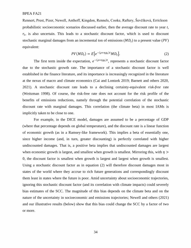
BPEA FA21


34

probabilistic socioeconomic scenarios discussed earlier, then the average discount rate to year t,

𝑟𝑡, is also uncertain. This leads to a stochastic discount factor, which is used to discount

stochastic marginal damages from an incremental ton of emissions (𝑀𝐷𝑡) to a present value (𝑃𝑉)

equivalent:

𝑃𝑉(𝑀𝐷𝑡) = 𝐸[𝑒−(𝜌+𝜂𝑔𝑡)𝑡𝑀𝐷𝑡]. (2)

The first term inside the expectation, 𝑒−(𝜌+𝜂𝑔𝑡)𝑡, represents a stochastic discount factor

due to the stochastic growth rate. The importance of a stochastic discount factor is well

established in the finance literature, and its importance is increasingly recognized in the literature

at the nexus of macro and climate economics (Cai and Lontzek 2019; Barnett and others 2020,

2021). A stochastic discount rate leads to a declining certainty-equivalent risk-free rate

(Weitzman 1998). Of course, the risk-free rate does not account for the risk profile of the

benefits of emissions reductions, namely through the potential correlation of the stochastic

discount rate with marginal damages. This correlation (the climate beta) in most IAMs is

implicitly taken to be close to one.

For example, in the DICE model, damages are assumed to be a percentage of GDP

(where that percentage depends on global temperature), and the discount rate is a linear function

of economic growth (as in a Ramsey-like framework). This implies a beta of essentially one,

since higher income (and, in turn, greater discounting) is perfectly correlated with higher

undiscounted damages. That is, a positive beta implies that undiscounted damages are largest

when economic growth is largest, and smallest when growth is smallest. Mirroring this, with 𝜂 >

0, the discount factor is smallest when growth is largest and largest when growth is smallest.

Using a stochastic discount factor as in equation (2) will therefore discount damages most in

states of the world where they accrue to rich future generations and correspondingly discount

them least in states where the future is poor. Amid uncertainty about socioeconomic trajectories,

ignoring this stochastic discount factor (and its correlation with climate impacts) could severely

bias estimates of the SCC. The magnitude of this bias depends on the climate beta and on the

nature of the uncertainty in socioeconomic and emissions trajectories; Newell and others (2021)

and our illustrative results (below) show that this bias could change the SCC by a factor of two

or more.

BPEA FA21


35

Despite the importance of stochastic discounting, federal government benefit-cost

analysis has historically not treated the discount rate as explicitly uncertain, nor has the discount

rate been connected to growth as in the Ramsey framework. Instead, the central discount rate

used in past government estimates of the SCC has been a constant rate of 3 percent.28 This is

equivalent to implicitly choosing the discounting parameters 𝜌 = 3% and 𝜂 = 0, corresponding

to a linear utility function. Yet this approach effectively eliminates any consideration of

declining discount rates, as in Weitzman (1998), and risk premia, as in Gollier (2014). More

intuitively, it also treats a $100 cost to a member of a wildly rich future generation the same as a

$100 cost to a poor one, which is incorrect from a welfare perspective. Correspondingly, such

parameter values receive little support from economists working in this field (Drupp and others

2018).

Although the case using stochastic discounting as in equation (1) is strong, the choice of

the parameters in that equation is not a simple matter, and their values can lead to very different

effective discount rates (e.g., Stern 2007; Nordhaus 2017a) and its connection to economic

growth and climate damages. One recent paper surveyed economists about their preferred values

of 𝜌 and 𝜂 (Drupp and others 2018). This is valuable, but the federal government has a long

tradition of relying on descriptive, empirical approaches to informing discounting guidance, as in

other aspects of benefit-cost analysis. In particular, Circular A-4 has referred to observed interest

rates in selecting 3 and 7 percent. A choice of 𝜌 and 𝜂 might therefore sensibly start with the

constraint that the associated near-term rate match the consumption rate used elsewhere in

benefit-cost analysis, as recommended in NASEM (2017). However, a continuum of (𝜌, 𝜂)

combinations can match any particular near-term rate, so another constraint is needed.

28 Although 3 percent was the central rate, the IWG also previously used constant rates of 2.5 and 5 percent

as sensitivity cases. Because those values were estimated to roughly approximate the effects of explicitly accounting

for uncertainty in risk-free and risk-adjusted rates (Newell and others 2021), those motivations are no longer

appropriate when stochastic discounting can be captured explicitly in the IAMs, as we propose.

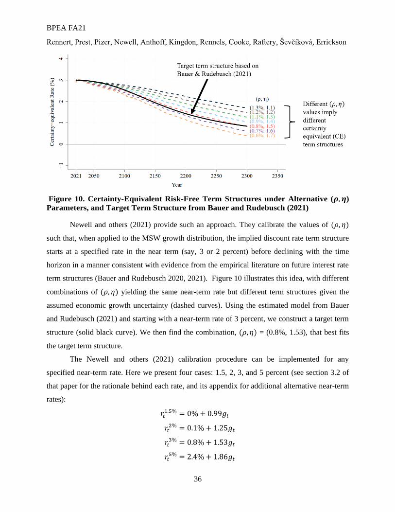
BPEA FA21


36

Figure 10. Certainty-Equivalent Risk-Free Term Structures under Alternative (𝝆, 𝜼)

Parameters, and Target Term Structure from Bauer and Rudebusch (2021)

Newell and others (2021) provide such an approach. They calibrate the values of (𝜌, 𝜂)

such that, when applied to the MSW growth distribution, the implied discount rate term structure

starts at a specified rate in the near term (say, 3 or 2 percent) before declining with the time

horizon in a manner consistent with evidence from the empirical literature on future interest rate

term structures (Bauer and Rudebusch 2020, 2021). Figure 10 illustrates this idea, with different

combinations of (𝜌, 𝜂) yielding the same near-term rate but different term structures given the

assumed economic growth uncertainty (dashed curves). Using the estimated model from Bauer

and Rudebusch (2021) and starting with a near-term rate of 3 percent, we construct a target term

structure (solid black curve). We then find the combination, (𝜌, 𝜂) = (0.8%, 1.53), that best fits

the target term structure.

The Newell and others (2021) calibration procedure can be implemented for any

specified near-term rate. Here we present four cases: 1.5, 2, 3, and 5 percent (see section 3.2 of

that paper for the rationale behind each rate, and its appendix for additional alternative near-term

rates):

𝑟𝑡1.5% = 0%+ 0.99𝑔𝑡

𝑟𝑡2% = 0.1% + 1.25𝑔𝑡

𝑟𝑡3% = 0.8% + 1.53𝑔𝑡

𝑟𝑡5% = 2.4% + 1.86𝑔𝑡

BPEA FA21


37

As discussed in Newell and others (2021), these 𝜌 and 𝜂 parameters lie in the middle of

the range often used in the literature, particularly for the central rates of 3 and 2 percent.

Implementing them simultaneously with the socioeconomic trajectories discussed in section II

produces a declining term structure of certainty-equivalent, risk-free rates consistent with the

empirical literature (Bauer and Rudebusch 2020, 2021). Importantly, implementing the

stochastic discount rate alongside stochastic damages via equation (2) explicitly captures risk

aversion and the correlation between the discount rate and climate damages, meaning no ex post

risk adjustment to the discount rate is necessary.

This calibrated stochastic discounting rule can now be used with the undiscounted

damage estimates (discussed above) to estimate the SCC in an internally consistent manner.

V. Illustrative Calculations of the Social Cost of Carbon

We present illustrative estimates of the SCC based on our socioeconomic projections (the

RFF-SPs), the FaIR climate model, and our discounting methodology—all of which speak

directly to the NASEM (2017) recommendations—and apply them using the DICE damage

function (Nordhaus 2017a). This approach is directly responsive to three of the four NASEM

recommendations. The fourth recommendation is to update the damage functions with the best

available science on sectoral damages, rather than using an aggregate damage function such as

that in DICE. We will include more recent sector-specific damage estimates, reflecting the best

available science, in future work, but for the moment we use the DICE damage function to

produce illustrative SCC estimates. Although the values we present here should be considered

illustrative, they highlight the importance of socioeconomic uncertainty and stochastic growth

discounting, and the interaction of these two important drivers of the SCC.

We also compare our SCC estimates with those from SSPs 1, 2, 3, and 5. Because of the

lack of socioeconomic uncertainty in each SSP—and the lack of relative probabilities across

them—we cannot meaningfully calibrate 𝜌 and 𝜂 parameters for those scenarios to deliver

BPEA FA21


38

comparable near-term rates. We therefore apply constant discount rates of 2 and 3 percent to the

SSPs.29

The results are shown in Figure 11, leading to our first major conclusion: a quantitative

probabilistic accounting of socioeconomic uncertainty matters greatly for the SCC. The top

panel of Figure 11 shows the distributions of our illustrative SCC values calibrated to 2 and 3

percent discount rates in the near term (means are also in the left columns of Table 1). The

bottom two panels show the SCC distributions under each SSP at 3 percent (left panel) and 2

percent (right panel) discount rates. The top panel reflects socioeconomic uncertainty implicitly,

leading to central SCC estimates of $56 and $171/ton CO2 under 3 and 2 percent near-term

stochastic discounting, respectively. The distribution underlying those means reflects both

socioeconomic and climate uncertainty. We disaggregate that distribution below, but the bottom

panel shows the importance of socioeconomic uncertainty explicitly by comparing across the

SSPs. SSP5 (high income growth) produces mean SCC values three to six times higher than the

other SSPs. Hence, if one were to use a weighted combination of the SSPs, the resulting average

SCC would reflect the relative weight given to each SSP, especially SSP5—a choice with no

clear empirical basis. This result highlights the importance of incorporating a quantitative

accounting of economic uncertainty, as in the RFF-SPs.

Next, Figure 12 demonstrates the effect of stochastic versus constant discounting on the

mean SCC, leading to our second major conclusion: stochastic growth discounting is crucially

important to SCC estimation in the context of socioeconomic uncertainty. The first two columns

of the first row show mean SCCs under the RFF-SPs for stochastic growth discounting

approaches consistent with 3 and 2 percent near-term rates (both in 2020 dollars), producing

mean SCC estimates of $56 and $171/ton CO2, respectively. These estimates, reflecting the

updated socioeconomic, emission, climate, and discounting modules (three of the four NAS

recommendations), are 22% and 53% higher than the corresponding DICE-only SCC estimates

from the 2016 IWG ($46 and $112/ton CO2 in 2020$, see RFF and NYSERDA 2020).

29 As an additional comparison, Figure OA-13 of the online appendix presents an analogous figure to

Figure 11 but applying our RFF-SP-calibrated discounting parameters (𝜌,𝜂) to the SSPs. This is purely for

presentational purposes, and we caution that our discounting parameters were not calibrated to the SSPs. Because

the SSPs have no uncertainty within them, it is not possible to calibrate discounting parameters to them as we can do

to the socioeconomic distributions (Newell and others 2021).

BPEA FA21


39

We also present the results from the RFF-SPs with constant discounting to illustrate the

importance of stochastic discounting, but as previously discussed, constant discounting is

inappropriate when uncertainty in economic growth is considered, as here. When constant

discounting is coupled with uncertain growth, the mean SCC is higher than is appropriate by a

factor of two to five, $125 and $785/ton CO2 for 3 and 2 percent discount rates, respectively,

because it ignores the correlation between damages and growth (the climate beta) and hence the

discount rate. In other words, ignoring the risk profile of the SCC threatens to overstate the mean

SCC in this example by a factor of two or more ($125 versus $56/ton with 3 percent discounting,

and $785 versus $171/ton with 2 percent discounting).

More specifically, the high expected values reflect a right-skewed distribution of

damages. It is well known that skewed distributions and tail events can influence the expected

value of the benefits of mitigating climate change (e.g., Gollier 2008; Weitzman 2011, 2014).

Under constant discounting, such tail events are very rich futures with associated large amounts

of consumption at risk from climate change. Yet constant discounting treats each dollar of cost to

those wealthy future generations the same as a dollar of cost to a relatively poor future. Hence,

with constant discounting, the effects on the future rich inappropriately dominate the expected

value of the SCC, leading to a strong upward bias in the SCC estimate.

This problem is recognized in the finance literature as the result of ignoring the risk

properties of an investment—namely, the correlation of an uncertain payoff with the stochastic

discount rate. Stochastic growth discounting addresses this by discounting the high-growth, high-

damage states at a higher rate. By discounting high-growth states more, stochastic discounting

stabilizes the mean and variance of the SCC, as documented in Newell and others (2021).

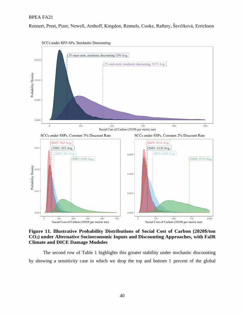
BPEA FA21


40

Figure 11. Illustrative Probability Distributions of Social Cost of Carbon (2020$/ton

CO2) under Alternative Socioeconomic Inputs and Discounting Approaches, with FaIR

Climate and DICE Damage Modules

The second row of Table 1 highlights this greater stability under stochastic discounting

by showing a sensitivity case in which we drop the top and bottom 1 percent of the global

BPEA FA21


41

average income trajectories.30 Under constant discounting, the mean SCC is quite sensitive to

dropping these 1 percent extremes, falling from $125 to $85/ton at a 3 percent discount rate and

from $785 to $371/ton at a 2 percent discount rate. By contrast, the mean SCC is virtually

unchanged under stochastic discounting, changing by less than 0.5 percent for each of the

stochastic rates that are consistent with 2 and 3 percent near-term rates. More generally, the

SCCs with stochastic discounting change only negligibly even when much larger percentiles are

dropped from the tails. For example, with stochastic discounting, the mean SCCs change by less

than 1 percent even when the top and bottom 10 percent of draws of global average income

trajectories are dropped, whereas under constant discounting, the mean SCCs fluctuate by factors

of two to four. This result highlights the stabilizing effect of properly incorporating stochastic

growth discounting, as anticipated in the NASEM (2017) report.

This stability with stochastic discounting is apparent in Figure 12, which plots the

individual Monte Carlo SCC draws against each draw’s long-run (2020–2300) global GDP per

capita growth rate, under the 3 percent near-term stochastic discounting parameters (𝜌 = 0.8%,

𝜂 = 1.53).31 Roughly speaking, the vertical spread of SCC values in the figure largely reflects

climate uncertainty for each given level of growth in GDP per capita, whereas the horizontal

spread of SCC values reflects uncertainty in long-run income growth. Because the DICE damage

function is proportional to GDP, undiscounted marginal damages scale roughly one-for-one with

income growth, but with 𝜂 > 1 they are discounted somewhat more than one-for-one with

stochastic discounting, leading to a modest negative relationship between the SCC and GDP per

capita growth. In other words, the SCC is higher when income growth is lower, and vice versa.

30 Specifically, we drop the draws with global average GDP per capita in 2300 in the top 1 percent and

bottom 1 percent of draws, before taking the average SCC. 31 The shape of the curve is similar under the 2 percent near-term parameters (𝜌 = 0.1%, 𝜂 = 1.25) but

shifted up to a higher level.

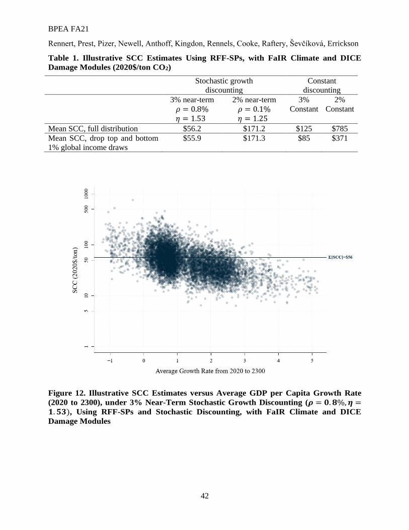
BPEA FA21


42

Table 1. Illustrative SCC Estimates Using RFF-SPs, with FaIR Climate and DICE

Damage Modules (2020$/ton CO2)

Stochastic growth

discounting

Constant

discounting

3% near-term

𝜌 = 0.8% 𝜂 = 1.53

2% near-term

𝜌 = 0.1% 𝜂 = 1.25

3%

Constant

2%

Constant

Mean SCC, full distribution $56.2 $171.2 $125 $785

Mean SCC, drop top and bottom

1% global income draws

$55.9 $171.3 $85 $371

Figure 12. Illustrative SCC Estimates versus Average GDP per Capita Growth Rate

(2020 to 2300), under 3% Near-Term Stochastic Growth Discounting (𝝆 = 𝟎. 𝟖%,𝜼 =𝟏. 𝟓𝟑), Using RFF-SPs and Stochastic Discounting, with FaIR Climate and DICE

Damage Modules

BPEA FA21


43

VI. Conclusion

Since the SCC is a vitally important metric guiding climate policy, its calculation must be

supported by the best available science, including an explicit incorporation of uncertainty. Our

results demonstrate that socioeconomic uncertainty and stochastic discounting are important

drivers of the SCC, and our work presents an opportunity to incorporate those uncertainties into

ongoing updates.

Although the SCC estimates presented here are meant to be illustrative and use a highly

simplified estimate of climate damages, they nonetheless highlight two major conclusions. First,

socioeconomics matter significantly to the SCC, highlighting the importance of a quantitative

accounting of socioeconomic uncertainty. Whereas scenario-based socioeconomic projections

like the SSPs have no formal probabilities attached to them, our approach to quantifying

uncertainties in future trajectories of population, GDP, and emissions helps account for these

uncertainties in the SCC. Second, when incorporating socioeconomic uncertainty, stochastic

growth discounting is crucial to account for the correlation of climate damages and the discount

rate, whereas ignoring it leads to a large upward bias in the SCC estimate. Our work represents

an advance in uncertain socioeconomic trajectories and discounting approaches based on

empirically based explicitly probabilistic methods. Nevertheless, potentially important

components have not yet been fully incorporated into officially adopted SCC values. Recent

work has begun to account for how the risk of tipping points influences the SCC (Dietz and

others 2021). Other important factors include climate-related migration, conflict, and loss of at-

risk species. Another conceptual issue is equity weighting, wherein effects on poorer regions of

the world could be weighted more than equivalently sized dollar-value to rich regions (Errickson

and others 2021). Future research in these areas could be incorporated into official SCC values

over time.

More generally, the SCC should be continually updated as the scientific frontier

advances, as recommended by NASEM (2017). Our work speaks directly to those NASEM

recommendations and presents an opportunity for the US government to improve on simple,

deterministic approaches to socioeconomic projections and discounting methodologies to better

reflect the interrelated uncertainties about future population, income, emissions, climate, and

discount rates.

BPEA FA21


44

ACKNOWLEDGMENTS We thank Lauren Dunlap, Jordan Wingenroth, and Anagha

Komaragiri for their expert assistance in preparing this manuscript. We gratefully acknowledge

the time and insights of the participants in our Expert Workshop on Very Long-Term Projections

of Population (Juha Alho, Leontine Alkema, Jakub Bijak, Patrick Gerland, Nico Keilman,

Ronald Lee, Jim Oeppen, Warren Sanderson, Tomas Sobotka); Economic Growth Survey (Daron

Acemoglu, Erik Brynjolfsson, Jean Chateau, Melissa Dell, Robert Gordon, Mun Ho, Chad Jones,

Pietro Peretto, Lant Pritchett, Dominique van der Mensbrugghe); and Future Emissions Survey

(Sally Benson, Geoff Blanford, Leon Clarke, Elmar Kriegler, Jennifer Faye Morris, Sergey

Paltsev, Keywan Riahi, Susan Tierney, Detlef van Vuuren). The work of Raftery and Ševčíková

was supported by NIH grant R01 HD070936 from the Eunice Kennedy Shriver National Institute

of Child Health and Human Development. RFF’s work under the Social Cost of Carbon

Initiative has been supported by the Alfred P. Sloan Foundation, the Hewlett Foundation, and

individuals donors.

References

Alkema, Leontine, Adrian E. Raftery, Patrick Gerland, Samuel J. Clark, François Pelletier,

Thomas Buettner, and Gerhard K. Heilig. 2011. Probabilistic Projections of the Total

Fertility Rate for All Countries. Demography 48(3): 815–39.

https://doi.org/10.1007/s13524-011-0040-5.

Arrow, Kenneth J., Maureen L. Cropper, Christian Gollier, Ben Groom, Geoffrey M. Heal,

Richard G. Newell, William D. Nordhaus. 2014. Should Governments Use a Declining

Discount Rate in Project Analysis? Review of Environmental Economics and Policy 8(2):

145–63. https://doi.org/10.1093/reep/reu008.

Ashwin, R., Carleton, T., Delgado, M., Greenstone, M., Houser, T., Hsiang, S., Hultgren, A.,

Jina, A., Kopp, R., McCusker, K. E., Nath, I., Rising, J., and Yuan, J. Estimating a Social

Cost of Carbon for Global Energy Consumption. Nature (in press).

Azose, Jonathan J., and Adrian E. Raftery. 2015. Bayesian Probabilistic Projection of

International Migration. Demography 52(5): 1627–50. https://doi.org/10.1007/s13524-

015-0415-0.

Azose, Jonathan J., Hana Ševčíková, and Adrian E. Raftery. 2016. Probabilistic Population

Projections with Migration Uncertainty. Proceedings of the National Academy of

Sciences of the United States of America 113(23): 6460–65.

https://doi.org/10.1073/pnas.1606119113.

BPEA FA21


45

Barnett, Michael, William Brock, and Lars Peter Hansen. 2020. Pricing Uncertainty Induced by

Climate Change. Review of Financial Studies 33(3): 1024–66.

https://doi.org/10.1093/rfs/hhz144.

———. 2021. Climate Change Uncertainty Spillover in the Macroeconomy. In NBER

Macroeconomics Annual 2021, Volume 36. University of Chicago Press.

https://www.nber.org/books-and-chapters/nber-macroeconomics-annual-2021-volume-

36/climate-change-uncertainty-spillover-macroeconomy.

Barrage, Lint. 2020a. Optimal Dynamic Carbon Taxes in a Climate–Economy Model with

Distortionary Fiscal Policy. Review of Economic Studies 87(1): 1–39.

https://doi.org/10.1093/restud/rdz055.

———. 2020b. The Fiscal Costs of Climate Change. AEA Papers and Proceedings 110 (May):

107–12. https://doi.org/10.1257/pandp.20201082.

Bauer, Michael, and Glenn Rudebusch. 2020. Interest Rates under Falling Stars. American

Economic Review 110(5): 1316–54. https://doi.org/10.1257/aer.20171822.

———. 2021. The Rising Cost of Climate Change: Evidence from the Bond Market. Review of

Economics and Statistics forthcoming.

Borenstein, Severin, James Bushnell, Frank A. Wolak, and Matthew Zaragoza-Watkins. 2019.

Expecting the Unexpected: Emissions Uncertainty and Environmental Market Design.

American Economic Review 109(11): 3953–77. https://doi.org/10.1257/aer.20161218.

Bradford, David F. 1975. Constraints on Government Investment Opportunities and the Choice

of Discount Rate. American Economic Review 65(5): 887–99.

Bressler, R. Daniel. 2021. The Mortality Cost of Carbon. Nature Communications 12(1): 4467.

https://doi.org/10.1038/s41467-021-24487-w.

Caballero, Ricardo J., Emmanuel Farhi, and Pierre-Olivier Gourinchas. 2017. Rents, Technical

Change, and Risk Premia Accounting for Secular Trends in Interest Rates, Returns on

Capital, Earning Yields, and Factor Shares. American Economic Review 107(5): 614–20.

https://doi.org/10.1257/aer.p20171036.

Cai, Yongyang, and Thomas S. Lontzek. 2019. The Social Cost of Carbon with Economic and

Climate Risks. Journal of Political Economy 127(6): 2684–2734.

https://doi.org/10.1086/701890.

Calvin, Katherine, Bryan K. Mignone, Haroon S. Kheshgi, Abigail C. Snyder, Pralit Patel,

Marshall Wise, Leon E. Clarke, and Jae Edmonds. 2020. Global Market and Economic

Welfare Implications of Changes in Agricultural Yields Due to Climate Change. Climate

Change Economics 11(01): 2050005. https://doi.org/10.1142/S2010007820500050.

Carleton, Tamma, Michael Delgado, Michael Greenstone, Trevor Houser, Solomon Hsiang,

Andrew Hultgren, Amir Jina, and others 2018. Valuing the Global Mortality

Consequences of Climate Change Accounting for Adaptation Costs and Benefits. SSRN

Scholarly Paper ID 3224365. Rochester, NY: Social Science Research Network.

https://papers.ssrn.com/abstract=3224365.

BPEA FA21


46

Carleton, Tamma, and Michael Greenstone. 2021. Updating the United States Government’s

Social Cost of Carbon. https://papers.ssrn.com/sol3/papers.cfm?abstract_id=3764255.

Christensen, Jens H. E., and Glenn D. Rudebusch. 2019. A New Normal for Interest Rates?

Evidence from Inflation-Indexed Debt. Review of Economics and Statistics 101(5): 933–

49. https://doi.org/10.1162/rest_a_00821.

Christensen, Peter, Kenneth Gillingham, and William D. Nordhaus. 2018. Uncertainty in

Forecasts of Long-Run Economic Growth. Proceedings of the National Academy of

Sciences 115(21): 5409–14. https://doi.org/10.1073/pnas.1713628115.

Clarke, Leon, Jiyong Eom, Elke Hodson Marten, Russell Horowitz, Page Kyle, Robert Link,

Bryan K. Mignone, Anupriya Mundra, and Yuyu Zhou. 2018. Effects of Long-Term

Climate Change on Global Building Energy Expenditures. Energy Economics 72 (May):

667–77. https://doi.org/10.1016/j.eneco.2018.01.003.

Clarke, Leon, and John Weyant. 2009. Introduction to the EMF 22 Special Issue on Climate

Change Control Scenarios. Energy Economics, International, U.S. and E.U. Climate

Change Control Scenarios: Results from EMF 22, 31 (December): S63.

https://doi.org/10.1016/j.eneco.2009.10.014.

Colson, Abigail R., and Roger M. Cooke. 2017. Cross Validation for the Classical Model of

Structured Expert Judgment. Reliability Engineering & System Safety 163 (July): 109–20.

https://doi.org/10.1016/j.ress.2017.02.003.

———. 2018. Expert Elicitation: Using the Classical Model to Validate Experts’ Judgments.

Review of Environmental Economics and Policy 12(1): 113–32.

https://doi.org/10.1093/reep/rex022.

Commoner, Barry. 1972. The Environmental Cost of Economic Growth. Population, Resources

and the Environment.

Cooke, Roger M. 1991. Experts in Uncertainty: Opinion and Subjective Probability in Science.

New York: Oxford University Press.

———. 2013. Uncertainty Analysis Comes to Integrated Assessment Models for Climate

Change … and Conversely. Climatic Change 117(3): 467–79.

https://doi.org/10.1007/s10584-012-0634-y.

Cooke, Roger M., Deniz Marti, and Thomas Mazzuchi. 2021. Expert Forecasting with and

without Uncertainty Quantification and Weighting: What Do the Data Say? International

Journal of Forecasting 37(1): 378–87. https://doi.org/10.1016/j.ijforecast.2020.06.007.

Council of Economic Advisers (CEA). 2017. Discounting for Public Policy: Theory and Recent

Evidence on the Merits of Updating the Discount Rate. Issue Brief.

https://obamawhitehouse.archives.gov/sites/default/files/page/files/201701_cea_discounti

ng_issue_brief.pdf.

Csiszar, I. 1975. Divergence Geometry of Probability Distributions and Minimization Problems.

Annals of Probability 3(1): 146–58.

BPEA FA21


47

Del Negro, Marco, Domenico Giannone, Marc P. Giannoni, and Andrea Tambalotti. 2017.

Safety, Liquidity, and the Natural Rate of Interest. Brookings Papers on Economic

Activity 2017(1): 235–316. https://doi.org/10.1353/eca.2017.0003.

Diaz, Delavane B. 2016. Estimating Global Damages from Sea Level Rise with the Coastal

Impact and Adaptation Model (CIAM). Climatic Change 137(1–2): 143–56.

https://doi.org/10.1007/s10584-016-1675-4.

Diaz, Delavane B., and Frances Moore. 2017a. Quantifying the Economic Risks of Climate

Change. Nature Climate Change 7(11): 774–82. https://doi.org/10.1038/nclimate3411.

Dietz, Simon, Christian Gollier, and Louise Kessler. 2018. The Climate Beta. Journal of

Environmental Economics and Management 87 (January): 258–74.

https://doi.org/10.1016/j.jeem.2017.07.005.

Dietz, Simon, James Rising, Thomas Stoerk, and Gernot Wagner. 2021. Economic Impacts of

Tipping Points in the Climate System. Proceedings of the National Academy of Sciences

118(34). https://doi.org/10.1073/pnas.2103081118.

Drèze, Jacques H. 1974. Discount Rates and Public Investment: A Post-Scriptum. Economica

41(161): 52–61. https://doi.org/10.2307/2553422.

Drupp, Moritz A., Mark C. Freeman, Ben Groom, and Frikk Nesje. 2018. Discounting

Disentangled. American Economic Journal: Economic Policy 10(4): 109–34.

https://doi.org/10.1257/pol.20160240.

Errickson, Frank, Keller, William D. Collins, Vivek Srikrishnan, and David Anthoff. 2021.

Equity Is More Important for the Social Cost of Methane than Climate Uncertainty.

Nature 592: 564–70.

Fosdick, Bailey, and Adrian E. Raftery. 2014. Regional Probabilistic Fertility Forecasting by

Modeling between-Country Correlations. Demographic Research 30(35): 1011–34.

https://doi.org/10.4054/DemRes.2014.30.35.

Gasparrini, Antonio, Yuming Guo, Francesco Sera, Ana Maria Vicedo-Cabrera, Veronika Huber,

Shilu Tong, Micheline de Sousa Zanotti Stagliorio Coelho, and others 2017. Projections

of Temperature-Related Excess Mortality under Climate Change Scenarios. Lancet

Planetary Health, November. https://doi.org/10.1016/S2542-5196(17)30156-0.

Gerland, Patrick, Adrian E. Raftery, Hana Sevčíková, Nan Li, Danan Gu, Thomas Spoorenberg,

Leontine Alkema, and others 2014. World Population Stabilization Unlikely This

Century. Science 346 (6206): 234–37. https://doi.org/10.1126/science.1257469.

Gietel-Basten, Stuart, Wolfgang Lutz, and Sergei Scherbov. 2013. Very Long Range Global

Population Scenarios to 2300 and the Implications of Sustained Low Fertility.

Demographic Research 28(39): 1145–66. https://doi.org/10.4054/DemRes.2013.28.39.

Giglio, Stefano, Matteo Maggiori, and Johannes Stroebel. 2015. Very Long-Run Discount Rates.

Quarterly Journal of Economics 130(1): 1–53. https://doi.org/10.1093/qje/qju036.

BPEA FA21


48

Giglio, Stefano, Matteo Maggiori, Johannes Stroebel, and Andreas Weber. 2015. Climate

Change and Long-Run Discount Rates: Evidence from Real Estate. Working Paper

21767. Cambridge, MA: National Bureau of Economic Research.

https://doi.org/10.3386/w21767.

Gollier, Christian. 2008. Discounting with Fat-Tailed Economic Growth. Journal of Risk and

Uncertainty 37(2–3): 171–86. https://doi.org/10.1007/s11166-008-9050-0.

———. 2014. Discounting and Growth. American Economic Review 104(5): 534–37.

https://doi.org/10.1257/aer.104.5.534.

Goulder, Lawrence H. 1995. Environmental Taxation and the Double Dividend: A Reader’s

Guide. International Tax and Public Finance 2(2): 157–83.

https://doi.org/10.1007/BF00877495.

Harberger, Arnold C. 1972. On Measuring the Social Opportunity Cost of Public Funds. In

Project Evaluation. Springer, 94–122.

Hausfather, Zeke, and Glen P. Peters. 2020. RCP8.5 Is a Problematic Scenario for Near-Term

Emissions. Proceedings of the National Academy of Sciences 117(45): 27791–92.


Ho, Emily, David V. Budescu, Valentina Bosetti, Detlef P. van Vuuren, and Klaus Keller. 2019.

Not All Carbon Dioxide Emission Scenarios Are Equally Likely: A Subjective Expert

Assessment. Climatic Change 155(4): 545–61. https://doi.org/10.1007/s10584-019-

02500-y.

Interagency Working Group on the Social Cost of Carbon (IWG SCC). 2010. Technical Support

Document: Technical Update of the Social Cost of Carbon for Regulatory Impact

Analysis Under Executive Order 12866. Washington, DC.

https://19january2017snapshot.epa.gov/sites/production/files/2016-

12/documents/sc_co2_tsd_august_2016.pdf.

———. 2021. Technical Support Document: Social Cost of Carbon, Methane, and Nitrous

Oxide Interim Estimates under Executive Order 1399. Interagency Working Group on

Social Cost of Greenhouse Gases, Washington, DC.

Johannsen, Benjamin K., and Elmar Mertens. 2016. A Time Series Model of Interest Rates With

the Effective Lower Bound. Finance and Economics Discussion Series 2016 (33): 1–46.

https://doi.org/10.17016/FEDS.2016.033.

Johnson, N. L. 1949. Systems of Frequency Curves Generated by Methods of Translation.

Biometrika 36(1/2): 149–76. https://doi.org/10.2307/2332539.

Kikstra, Jarmo, Paul Waidelich, James Rising, Dmitry Yumashev, Chris Hope, and Chris

Brierley. 2021. The Social Cost of Carbon Dioxide under Climate-Economy Feedbacks.

Environmental Research Letters forthcoming.

https://doi.org/10.13140/RG.2.2.34696.55044.

Kiley, Michael T. 2020. What Can the Data Tell Us about the Equilibrium Real Interest Rate?

International Journal of Central Banking 16(3): 181–209.

BPEA FA21


49

Kopp, Robert E., and Bryan K. Mignone. 2012. The U.S. Government’s Social Cost of Carbon

Estimates after Their First Two Years: Pathways for Improvement. Economics 6(1):

20120015. https://doi.org/10.5018/economics-ejournal.ja.2012-15.

Laubach, Thomas, and John C. Williams. 2016. Measuring the Natural Rate of Interest Redux |

SpringerLink. Business Economics 51: 57–67.

Leach, Nicholas J., Stuart Jenkins, Zebedee Nicholls, Christopher J. Smith, John Lynch,

Michelle Cain, Tristram Walsh, Bill Wu, Junichi Tsutsui, and Myles R. Allen. 2021.

FaIRv2.0.0: A Generalized Impulse Response Model for Climate Uncertainty and Future

Scenario Exploration. Geoscientific Model Development 14(5): 3007–36.

https://doi.org/10.5194/gmd-14-3007-2021.

Lemoine, Derek. 2021. The Climate Risk Premium: How Uncertainty Affects the Social Cost of

Carbon. Journal of the Association of Environmental and Resource Economists 8(1): 27–

57. https://doi.org/10.1086/710667.

Li, Qingran, and William A. Pizer. 2021. Use of the Consumption Discount Rate for Public

Policy over the Distant Future. Journal of Environmental Economics and Management

107 (May): 102428. https://doi.org/10.1016/j.jeem.2021.102428.

Liu, Peiran, and Adrian E. Raftery. 2020. Accounting for Uncertainty about Past Values in

Probabilistic Projections of the Total Fertility Rate for Most Countries. Annals of Applied

Statistics 14(2): 685–705. https://doi.org/10.1214/19-AOAS1294.

Liu, P. and Raftery, A.E. (2021). Country-based emissions reductions should increase by 80% beyond nationally determined contributions to meet the 2 C target. Communications Earth and Environment 2:Article 29.

Marglin, Stephen A. 1963a. The Opportunity Costs of Public Investment. Quarterly Journal of

Economics 77(2): 274–89. https://doi.org/10.2307/1884403.

———. 1963b. The Social Rate of Discount and The Optimal Rate of Investment. Quarterly

Journal of Economics 77(1): 95–111. https://doi.org/10.2307/1879374.

Millar, Richard J., Zebedee R. Nicholls, Pierre Friedlingstein, and Myles R. Allen. 2017. A

Modified Impulse-Response Representation of the Global Near-Surface Air Temperature

and Atmospheric Concentration Response to Carbon Dioxide Emissions. Atmospheric

Chemistry and Physics 17(11): 7213–28. https://doi.org/10.5194/acp-17-7213-2017.

Moore, Frances C., Uris Baldos, Thomas Hertel, and Delavane B. Diaz. 2017. New Science of

Climate Change Impacts on Agriculture Implies Higher Social Cost of Carbon. Nature

Communications 8(1). https://doi.org/10.1038/s41467-017-01792-x.

Müller, Ulrich K., James H. Stock, and Mark W. Watson. 2019. An Econometric Model of

International Long-Run Growth Dynamics. Working Paper 26593. Cambridge, MA:

National Bureau of Economic Research. https://doi.org/10.3386/w26593.

Müller, Ulrich K., and Mark W. Watson. 2016. Measuring Uncertainty about Long-Run

Predictions. Review of Economic Studies 83(4): 1711–40.

https://doi.org/10.1093/restud/rdw003.

BPEA FA21


50

National Academies of Sciences, Engineering, and Medicine (NASEM). 2017. Valuing Climate

Damages: Updating Estimation of the Social Cost of Carbon Dioxide. Washington, DC:

National Academies Press. https://doi.org/10.17226/24651.

Newell, Richard G., William A. Pizer, and Brian C. Prest. 2021. A Discounting Rule for the

Social Cost of Carbon. Working Paper. Washington, DC: Resources for the Future.

https://www.rff.org/publications/working-papers/a-discounting-rule-for-the-social-cost-

of-carbon/.

Nicholls, Zebedee R. J., Malte Meinshausen, Jared Lewis, Robert Gieseke, Dietmar Dommenget,

Kalyn Dorheim, Chen-Shuo Fan, and others 2020. Reduced Complexity Model

Intercomparison Project Phase 1: Introduction and Evaluation of Global-Mean

Temperature Response. Geoscientific Model Development 13(11): 5175–90.

https://doi.org/10.5194/gmd-13-5175-2020.

Nordhaus, William D. 1982. How Fast Should We Graze the Global Commons? American

Economic Review 72(2): 242–46.

———. 2017a. Revisiting the Social Cost of Carbon. Proceedings of the National Academy of

Sciences 114(7): 1518–23. https://doi.org/10.1073/pnas.1609244114.

———. 2017b. Evolution of Assessments of the Economics of Global Warming: Changes in the

DICE Model, 1992–2017. Working Paper 23319. Cambridge, MA: National Bureau of

Economic Research. https://doi.org/10.3386/w23319.

Oeppen, Jim, and James W. Vaupel. 2002. Demography. Broken Limits to Life Expectancy.

Science 296 (5570): 1029–31. https://doi.org/10.1126/science.1069675.

Pigou, Arthur C. 1920. The Economics of Welfare. Macmillan.

https://www.palgrave.com/gp/book/9780230249318.

Pizer, William A. 2021. A Shadow-Price-of-Capital Approach to Harmonize Discounting for

Greenhouse Gases in Broader Benefit-Cost Analyses.

https://media.rff.org/documents/OMB-2021-0006-0059_attachment_1.pdf

Prest, Brian C. 2021. Supply-Side Reforms to Oil and Gas Production on Federal Lands:

Modeling the Implications for Climate Emissions, Revenues, and Production Shifts.

Working Paper. Washington, DC: Resources for the Future.

https://www.rff.org/publications/working-papers/supply-side-reforms-oil-and-gas-

production-federal-lands/.

Prest, Brian C., and James H. Stock. 2021. Climate Royalty Surcharges. Working Paper.

Cambridge, MA: National Bureau of Economic Research.

https://www.nber.org/papers/w28564.

Preston, Samuel, Patrick Heuveline, and Michel Guillot. 2001. Demography: Measuring and

Modeling Population Processes. Malden, MA: Blackwell.

Rachel, Łukasz, and Lawrence H. Summers. 2019. On Falling Neutral Real Rates, FIscal Policy,

and the Risk of Secular Stagnation. Brookings Papers on Economic Activity. 68.

BPEA FA21


51

https://www.brookings.edu/bpea-articles/on-falling-neutral-real-rates-fiscal-policy-and-

the-risk-of-secular-stagnation/

Raftery, Adrian E. 2021. The Dip in the US Birthrate Isn’t a Crisis, but the Fall in Immigration

May Be. Conversation, June 21. http://theconversation.com/the-dip-in-the-us-birthrate-

isnt-a-crisis-but-the-fall-in-immigration-may-be-161169.

Raftery, Adrian E., Leontine Alkema, and Patrick Gerland. 2014a. Bayesian Population

Projections for the United Nations. Statistical Science : A Review Journal of the Institute

of Mathematical Statistics 29(1): 58–68. https://doi.org/10.1214/13-STS419.

Raftery, Adrian E., Nevena Lalic, and Patrick Gerland. 2014b. Joint Probabilistic Projection of

Female and Male Life Expectancy. Demographic Research 30(27): 795–822.

https://doi.org/10.4054/DemRes.2014.30.27.

Raftery, Adrian E., Jennifer L. Chunn, Patrick Gerland, and Hana Ševčíková. 2013. Bayesian

Probabilistic Projections of Life Expectancy for All Countries. Demography 50(3): 777–

801. https://doi.org/10.1007/s13524-012-0193-x.

Raftery, Adrian E., Nan Li, Hana Ševčíková, Patrick Gerland, and Gerhard K. Heilig. 2012.

Bayesian Probabilistic Population Projections for All Countries. Proceedings of the

National Academy of Sciences 109(35): 13915–21.


Raftery, Adrian E., and Hana Sevčíková. Forthcoming. Probabilistic Population Forecasting:

Short to Very Long-Term. International Journal of Forecasting.

Raftery, Adrian E., Alec Zimmer, Dargan M. W. Frierson, Richard Startz, and Peiran Liu. 2017.

Less than 2°C Warming by 2100 Unlikely. Nature Climate Change 7(9): 637–41.

https://doi.org/10.1038/nclimate3352.

Raimi, Daniel. 2021. Effects of Climate Change on Heat- and Cold-Related Mortality: A

Literature Review to Inform Updated Estimates of the Social Cost of Carbon. Working

Paper. Washington, DC: Resources for the Future.

https://www.rff.org/publications/working-papers/effects-of-climate-change-on-heat-and-

cold-related-mortality-a-literature-review-to-inform-updated-estimates-of-the-social-cost-

of-carbon/.

Ramsey, F. P. 1928. A Mathematical Theory of Saving. Economic Journal 38(152): 543–59.

https://doi.org/10.2307/2224098.

Resources for the Future (RFF) and New York State Energy Research and Development

Authority (NYSERDA). 2021. Estimating the Value of Carbon: Two Approaches. 2021.

https://www.rff.org/publications/reports/estimating-the-value-of-carbon-two-approaches/.

Riahi, Keywan, Detlef P. van Vuuren, Elmar Kriegler, Jae Edmonds, Brian C. O’Neill,

Shinichiro Fujimori, Nico Bauer, and others 2017. The Shared Socioeconomic Pathways

and Their Energy, Land Use, and Greenhouse Gas Emissions Implications: An Overview.

Global Environmental Change 42 (January): 153–68.

https://doi.org/10.1016/j.gloenvcha.2016.05.009.

BPEA FA21


52

Rose, Steven K., Delavane B. Diaz, and Geoffrey J. Blanford. 2017. Understanding the Social

Cost of Carbon: A Model Diagnostic and Inter-Comparison Study. Climate Change

Economics 8(2): 1750009. https://doi.org/10.1142/S2010007817500099.

Rose, Steven K., Delavene Turner, Geoffrey Blanford, John Bistline, Francisco C. de la

Chesnaye, and Tom Wilson. 2014. Understanding the Social Cost of Carbon: A

Technical Assessment. Electric Power Research Institute.

Sandmo, Agnar, and Jacques H. Drèze. 1971. Discount Rates for Public Investment in Closed

and Open Economies. Economica 38(152): 395–412. https://doi.org/10.2307/2551880.

Sjaastad, Larry A., and Daniel L. Wisecarver. 1977. The Social Cost of Public Finance. Journal

of Political Economy 85(3): 513–47. https://doi.org/10.1086/260582.

Stammer, Detlef, Anita Engels, Jochem Marotzke, Eduardo Gresse, Christopher Hedemann, and

Jan Petzold. 2021. Hamburg Climate Futures Outlook: Assessing the Plausibility of Deep

Decarbonization by 2050. https://doi.org/10.25592/uhhfdm.9104.

Stern, Nicholas. 2007. The Economics of Climate Change: The Stern Review. Cambridge:

Cambridge University Press. https://www.cambridge.org/us/academic/subjects/earth-and-

environmental-science/climatology-and-climate-change/economics-climate-change-stern-

review, https://www.cambridge.org/us/academic/subjects/earth-and-environmental-

science/climatology-and-climate-change.

United Nations. 2004. World Population to 2300. New York

https://www.un.org/development/desa/pd/sites/www.un.org.development.desa.pd/files/fil

es/documents/2020/Jan/un_2002_world_population_to_2300.pdf.

———. 2019. World Population Prospects: The 2019 Revision. New York.

Vallin, J and G. Caselli. 1997. Towards a New Horizon in Demographic Trends: The Combined

Effects of 150 Years Life Expectancy and New Fertility Models. In J. M. Robine, J. W.

Vaupel, B. Jeune, and M. Allard (eds), Longevity: To the Limits and Beyond.

Berlin/Heidelberg: Springer-Verlag, 29–68.

Weitzman, Martin L. 1998. Why the Far-Distant Future Should Be Discounted at Its Lowest

Possible Rate. Journal of Environmental Economics and Management 36(3): 201–208.

https://doi.org/10.1006/jeem.1998.1052.

———. 2011. Fat-Tailed Uncertainty in the Economics of Catastrophic Climate Change. Review

of Environmental Economics and Policy 5(2): 275–92.

https://doi.org/10.1093/reep/rer006.

———. 2014. Fat Tails and the Social Cost of Carbon. American Economic Review 104(5):

544–46. https://doi.org/10.1257/aer.104.5.544.

World Health Organization. 2014. Quantitative Risk Assessment of the Effects of Climate Change

on Selected Causes of Death, 2030s and 2050s. Geneva.

https://apps.who.int/iris/handle/10665/134014.

BPEA FA21

Rennert, Prest, Pizer, Newell, Anthoff, Kingdon, Rennels, Cooke, Raftery, Ševčíková, and

Errickson

Conflict of Interest Disclosure:

The Social Cost of Carbon: Advances in Long-term

Probabilistic Projections of Population, GDP, Emissions, and

Discount Rates

Online Appendix

I. Description of censoring of raw MSW economic growth dataset

As indicated in MSW (2019), there is considerable uncertainty in future economic growth

100-300 years into the future. As a result, the tails of the MSW distribution are quite wide, leading

to some implausibly small or implausibly large future levels of GDP per capita in the extreme tails

(e.g., below the 1st percentile or above the 99th percentile). These extreme tails correspond to

extremes of persistent economic growth beyond that which has been observed for any country in

the historical record over such long time periods (e.g., below -1% or above +5% annually on

average through 2300), but nonetheless are possible as simulated projections given the

distributional assumptions of the MSW model. Such low or high sustained growth rates would

lead to global GDP/capita either falling by more than 90% between 2021 and 2300 (e.g., 0.99279)

or rising by a factor of more than 800,000 (1.05279) implying a global average income of more than

$10 billion per person. However, according to the Maddison Project dataset,1 which includes

country-level GDP/capita data as far back as 1500 for some countries, no country has ever

experienced such extreme growth for such long periods of time.2 Further, the 1st and 99th

percentiles of the combined distribution of long-run growth rates based on the EGS are -0.6% and

+4.4%, indicating long-run growth rates are exceptionally unlikely to fall outside this range. In the

MSW model, those extreme tail outcomes are very likely driven by the structure of the Bayesian

1 Available at https://clio-infra.eu/Indicators/GDPperCapita.html 2 For example, no country in Maddison Project data has observed 100-year growth rates of below -1% or

above +3%,

https://clio-infra.eu/Indicators/GDPperCapita.html

BPEA FA21


Errickson

model, such as its embedded distributional assumptions, rather than the historical data used to

estimate the model.

For these reasons, and in consultation with James Stock (one of the authors of MSW

(2019)), we lightly censor some projections in the extreme tails of the MSW distribution that are

outside the range of historical experience and also outside the long-run range implied by the EGS,

using a combination of two approaches. We first use the Maddison Project data to calculate, for

each annual time horizon from 1 to 150 years, the minimum and maximum sustained growth rates

ever observed by any country historically over that time horizon. For example, at the 50-year time

horizon, these minimum and maximum rates were -2.4% (DR Congo, 1954-2004) and +7.0%

(Equatorial Guinea 1958-2008). While this approach is sufficient to establish bounds for horizons

up to 150 years into the future, it is less informative for the very long term (e.g., 150-300 years)

because the Maddison data has relatively few countries for such long time horizons. Therefore, we

augment these historical ranges using the range suggested by the extreme quantiles of the

combined growth distribution from the EGS. Specifically, we use as bounding values the 0.5th and

99.5th quantiles of the combined (performance-weighted) distribution of long-run (2020-2300)

growth rates from the EGS, which are -0.88% and +5.1%.

We use the outer envelope of (i.e., the less restrictive of) these two sets of bounding values

for growth for each time horizon from 1 to 300 years. Specifically, these bounds are calculated as

the outer envelope of the change in log(GDP/capita) implied by the horizon-specific growth rates

from the Maddison data and those implied by the EGS (-0.88% and +5.1% annually). Country-by-

year values in the projections that exceed these absorbing bounds are set equal to the bounds. This

affects less than one percent of country-by-year draws in each tail of the distribution. The time

paths of these absorbing bounds are shown in Figure OA-1.

BPEA FA21


Errickson

Figure OA- 1 Absorbing Bounds for Change in Country-Level GDP/capita Over

Time.

II. Structured Expert Judgment: Details on experts and scoring for

Economic Growth Survey (EGS) and Future Emissions Survey (FES)

1. Introduction

2. Expert scoring

3. Combining experts

4. Robustness

5. Random Expert Hypothesis

6. Range graphs

7. Conclusion

8. References

1. Introduction

BPEA FA21


Errickson

This report details on the structured expert judgment studies of GDP and greenhouse gas

emissions conducted by RFF as part of RFF’s activities to implement recommendations from the

National Academies of Sciences, Engineering, and Medicine (NASEM 2017) for improving

estimates of the social cost of carbon.

Ten experts participated in the Economic Growth Survey (EGS) in Washington DC in

2019-2020. Ten experts participated in the Future Emissions Survey (FES) elicitation also held at

RFF in 2021. From previous experience a working minimum panel size is about six experts and

more than 20 provides diminishing returns in terms of the performance of the pooled expert

judgments.

The participating experts in the EGS were: Daron Acemoglu, Erik Brynjolfsson, Jean

Chateau, Melissa Dell, Robert Gordon, Mun Ho, Chad Jones, Pietro Peretto, Lant Pritchett,

Dominique van der Mensbrugghe. The participating experts in the FES were: Sally Benson, Geoff

Blanford, Leon Clarke, Elmar Kriegler, Jennifer Faye Morris, Sergey Paltsev, Keywan Riahi,

Susan Tierney, Detlef van Vuuren. Elicitations were conducted face to face remotely. Experts

were provided with an introductory video and background materials to orient them to the study.

The expert judgment methodology applied here is termed the “Classical Model” because

of its analogy to classical hypothesis testing (1). The key idea is that experts are treated as statistical

hypotheses. They are scored as uncertainty assessors based on their responses to calibration

variables from their field whose true values are unknown to the experts at the time of the elicitation.

The purpose of scoring is twofold. First scoring enables performance weighted combinations of

experts’ judgments. Second, the scores of combinations of experts serve to gauge and hopefully

validate the combination which is adopted.

2. Expert scoring

Each expert stated his/her 5th , 50 th and 95 th percentiles, or quantiles, for each calibration

variable. An expert’s statistical accuracy is the P-value (column 2 in Tables 3 and 4) at which we

would falsely reject the hypothesis that an expert’s probability assessments are statistically

accurate. Roughly, an expert is statistically accurate if, in a statistical sense, 5% of the realizations

fall beneath his/her 5th percentile, 45% of the realizations fall between the 5th and 50th percentile,

etc. High values (near 1) are good, low values (near 0) reflect low statistical accuracy. An expert’s

BPEA FA21


Errickson

informativeness is measured as the mean Shannon relative information in the expert’s distribution

with respect to a uniform background measure over an interval containing all experts’ percentile

assessments and the realizations, variable-wise3.

Column 3 gives the average information scores for each expert for all variables. The

number of calibration variables is shown in column 4 for each expert (in this case all experts

assessed all 11 calibration variables). The product of columns 2 and 3 is the combined score for

each expert (not shown). Note that statistical accuracy scores vary over four orders of magnitude

whereas information scores vary within a factor two. Statistical accuracy is a fast function while

informativeness is slow. Therefore, by design, the ratios of the products of combined scores are

dominated by the statistical accuracy.

There is a loose negative correlation between experts’ statistical accuracy and information.

Note also that while the equal weight combination’s statistical accuracy in both panels is

comfortably above the 5% threshold, its information is lower than that of any expert. As

mentioned, information is a slow function; halving the information score corresponds roughly to

doubling the size of the 90 percent confidence bands. This information penalty of equal weighting

is typical of other expert judgment panels.

Six of the nine EGS experts had a statistical accuracy score above 0.05 which is the

traditional threshold below which statistical hypotheses would be rejected. For the FES panel this

holds for 5 of the 10 experts. A recent review of the 49 studies conducted since 2006 found that

75% of the 530 experts would be rejected as statistical hypotheses at the 5% level. In this sense,

both the EGS and the FES panels display an unusually high number of non-rejected experts. This

in turn leads to lower performance differences between equal and performance weighting than is

seen in many other studies.

3 Computing the mean relative information requires fitting densities to each experts’ quantile assessments.

The minimal informative density relative to the background measure which complies with the expert’s quantiles is

chosen for this purpose. The mean relative information is proportional to the information in each expert’s joint

distribution if the distributions for each variable are independent. The mean is taken to prevent the importance of

informativeness to depend on the number of calibration variables. The mean relative information is a global

performance measure; the actual weights employ the information scores per variable and are thus variable specific.

BPEA FA21


Errickson

Expert Scores EGS

expert

Statistical

accuracy

mean

information # variables weight

Rel.Inf to EW

DM

1 0.706 0.673 11 0.3 0.433

2 0.399 0.829 11 0.209 0.608

3 0.008 0.894 11 - 0.6

4 0.197 0.659 11 0.082 0.363

5 0.215 1.094 11 0.148 0.711

6 0.327 1.131 11 0.233 0.761

7 0.154 0.291 11 0.028 0.331

8 0.018 1.087 11 - 0.671

9 0.0003 0.727 11 - 0.511

PW05 0.492 0.457 11 -

EW 0.37 0.266 11 -

Table 1 Scores and weights for all 9 EGS experts when performance weights are

not optimized but computed for the six weighted experts with statistical accuracy > 0.05.

Statistical accuracy denotes the significance level at which the hypothesis that an expert

is statistically accurate would be falsely rejected. Mean Information denotes the average

Shannon relative information in an expert’s assessments for all calibration variables. “#

variabless” denotes the number of calibration variables answered by an expert.

“Weight” for weighted experts is the normalized sum of the product of columns 2 and 3.

“Rel Inf to EW DM” is an expert’s relative information with respect to the EW

combination of all experts.

BPEA FA21


Errickson

Expert Scores FES

expert Statistical accuracy

mean information

# variables

weight (GWnOp)

Rel.Inf to EW DM

1 0.083 0.893 11 0.079 0.636

2 1.26E-05 1.354 11 0.000 1.003

3 1.70E-07 1.592 11 0.000 1.182

4 3.01E-04 1.357 11 0.000 1.271

5 0.003 1.295 11 0.005 0.935

6 0.399 0.548 11 0.234 0.400

7 0.018 0.748 11 0.015 0.649

8 0.169 0.676 11 0.122 0.460

9 0.327 0.846 11 0.295 0.601

10 0.385 0.611 11 0.251 0.408

GWnOp 0.615 0.308 11 0.006

GWOp 0.852 0.313 11 0.043 IWnOp 0.385 0.361 11 0.042

IWOp 0.615 0.361 11 0.210

EW 0.638 0.238 11 0

Table 2: Scores and weights for all 10 FES experts when performance weights are

optimized (Op) and also not optimized (nOP, no statistical accuracy cut-off is applied). The

weights in column 5 are those of GWnOP. Global weighting (GW) uses the mean

informativeness over all calibration variables. Statistical accuracy denotes the significance

level at which the hypothesis that an expert is statistically accurate would be falsely rejected.

Mean Information denotes the average Shannon relative information in an expert’s

assessments for all calibration variables. “# variables” denotes the number of calibration

variables answered by an expert. “Global Weight” for weighted experts is the normalized

sum of the product of columns 2 and 3. Item specific weighting (IW) applies different weights

for each item based on an experts’ informativeness per item. “Rel Inf to EW DM” is an

expert’s relative information with respect to the EW combination of all experts.

BPEA FA21


Errickson

3. Combining experts

A scoring system is asymptotically strictly proper if an expert obtains his/her highest

expected score in the long run by, and only by, stating percentiles corresponding to his/her true

beliefs. Statistical accuracy and informativeness are dimensionless. Their product termed the

combined score, is an asymptotically strictly proper scoring rule if experts get zero weight when

their P-value drops below some positive threshold (1). If (s)he tries to game the system to

maximize his/her expected weight, (s)he will eventually figure out that (s)he must say exactly what

(s)he thinks. Honesty is the only optimal strategy. The theory does not say what the cut-off value

should be, so this is chosen on the basis of extra-mathematical considerations. One strategy is to

choose the cut-off at the level which optimizes the combined score of the resulting decision maker.

Another strategy is to choose a statistical cutoff, typically 0.05, such that weighted experts are

those would not be rejected as statistical hypotheses. A third strategy is to choose a cutoff

sufficiently low that all empanelled experts are weighted (termed not optimized or nOp).

For the EGS, optimal weighting resulted in expert 1 receiving weight one, other experts

being unweighted. The strategy cutoff strategy choosing the cutoff at the traditional 5% value,

termed PW05 shown in Table 2. All three DM’s EW, PWOp and PW05 show acceptable statistical

performance4. EW exhibits lower informativeness than any expert and lower than PWOp and

PW05. Very roughly, halving the informativeness corresponds to doubling the width of the 90%

confidence intervals. In this case PWOpt was rather non robust whereas PW05 was very robust

(see below).

For the FES there was very little difference in performance between IWOp, IWnOp,

GWOp and GWnOp. All are more informative than EW. Optimization incurs a penalty in

robustness (see below) and in light of the small differences in performances, preference was given

for the non-optimized versions.

The Classical Model has been applied in hundreds of expert panels and has been validated

both in- and out-of-sample (2-6). In the absence of observations of the variables of interest, out-

of-sample validation comes down to cross-validation whereby the calibration variables are

repeatedly separated into subsets of training- and test variables. The PW model is initialized on

4 If an expert is statistically accurate, then his/her statistical accuracy score is uniformly distributed on the

interval [0, 1] and small values are significant. A difference between 0.4 and 0.5 is not important, but a difference of

0.4 and 0.008 is.

BPEA FA21


Errickson

the training variables and scored on the test variables. The superiority of PW over EW in terms of

statistical accuracy and informativeness has been demonstrated using this approach (2).

4. Robustness

Robustness on experts examines the effect on the preferred combination of losing

individual experts. For the EGS panel, experts are removed one at a time and PW05 is recomputed

as shown in Table 3.

Robustness analysis on Experts

Excluded

expert

Information wrt

background

Statistical

accuracy

Information wrt original

DM

1 0.524 0.492 0.106

2 0.511 0.370 0.105

3 0.428 0.492 0.007

4 0.478 0.492 0.057

5 0.445 0.492 0.037

6 0.424 0.492 0.054

7 0.391 0.492 0.043

8 0.451 0.492 0.003

9 0.393 0.492 0.011

Table 3. Robustness on EGS experts; for explanations of columns see section 1.2,

“Information wrt original DM” gives the mean relative information of the perturbed

DM (with one expert removed) with respect to the original DM.

Table 4 shows that the mean relative information with respect to the original PW05 is in

the order 0.05. Comparison with the values in the rightmost column of Table 2 shows that the

changes wrought in PW05 by loss of a single expert are much smaller than the differences among

the experts themselves. In this sense we conclude that PW05 is robust against the loss of any single

expert. Had we chosen PWOpt, the difference caused by losing the expert with weight 1 would

be 0.56, which is on the order of the expert differences.

BPEA FA21


Errickson

Robustness against loss of a calibration variable proceeds in the same manner. Calibration

variables are removed one at a time and PW05 is recomputed. These scores are extremely robust

against loss of a calibration variable. A calibration variable may exert leverage on the combination

of experts if all experts assess this variable poorly. That may be due to “group think” or it may be

due to inappropriateness, ambiguity or error in the true value. If one variable perturbs the

combination more than the others, this flags the variable in question for further scrutiny. Table 5

raises no flags in this regard. Comparing the rightmost columns of Tables 1 and 5 show that the

perturbation caused by loss of a single calibration variable is small relative to the divergence

among the experts themselves.

Robustness analysis on variables

Excluded

variable

Information

wrt

background

Statistical

accuracy

Information

wrt original

DM

GrwCh 0.44 0.47 0.04

GrwSA 0.49 0.47 0.04

GrwSSA 0.44 0.47 0.05

MADCh 0.41 0.55 0.06

MADSA 0.51 0.55 0.05

MADSSA 0.52 0.47 0.05

CBOErr 0.45 0.55 0.04

$StLIC 0.38 0.47 0.04

$StHIC 0.45 0.55 0.02

DyCLIC 0.47 0.55 0.04

DyCHIC 0.50 0.47 0.05

Table 4: Robustness on EGS calibration questions (calib vbl); for explanations of

columns see section 1.2. “Information wrt original DM” gives the mean relative

information of the perturbed DM (with one expert removed) with respect to the original

DM.

BPEA FA21


Errickson

For the optimized combinations in the FES panel the results are non-robust against both

loss of a calibration variable and loss of an expert. This information is combined in a single table

below.

excluded expert Rel Inf wrt PWnOp

rel inf wrt GWOp Excluded item

Rel Inf wrt PWnOp

rel inf wrt GWOp

1 0.01695 0.2578 spAdEc 0.0131 0.04904

2 2.51E-06 3.39E-09 spEmMr 0.0231 0.298 3 1.79E-07 0 spEaPc 0.02474 0.2561 4 0.006481 0.2578 %OECD 0.0144 0.3188

5 0.001533 2.67E-08 %SSAf 0.07927 0.04931 6 0.08502 0.1604 #ngSA 0.07836 0.3087 7 0.009123 0.06184 #ngSSA 0.01785 0.3204

8 0.0172 0.03377 %ergME 0.06166 0.4397 9 0.04194 0.2578 %ergCh 0.02913 0.2442

10 0.07871 0.08283 RnwVen 0.05453 0.06587 RwnPor 0.02095 0.3209

Table 5. Robustness on FES experts and items for optimized vs non optimized

global weights.

5. Random Expert Hypothesis

The random expert hypothesis states that putative differences in performance between

assessors is just noise and does not indicate persistent differences of the assessors (6). One way to

test this hypothesis is to compare panel wide performance metrics in the original panel with the

same metrics as generated by a large set (here 1000) of “scrambled panels” in which the

assessments are randomly re-allocated to assessors, thus wiping out any ‘assessor effect’.

Considering statistical accuracy (SA) and information (Inf), we are interested in the panel maxima,

minima averages and standard deviations. Table 6 shows, for example, that the average SA score

in the original EGS panel was 0.23. In 14.1% of the 1000 scrambled panels the average SA score

was lower than 0.23. The minimum SA score in the original EGS panel was 0.0003 and in all 1000

scrambled panels the minimum SA score was greater than the original panel minimum Sa.

Although the scrambling was able to exceed the panel average SA in 85.9% of the cases, it was

BPEA FA21


Errickson

never able to get scores as low as the minimum in the original panel. The average Inf score is

always the same in the scrambled and original panels, but the scrambling was unable to reproduce

the highest and lowest scores. The same pattern is observed in the second panel. The fact that

significant departures from randomness (indicated by italicized values) do not occur for average

or maximum values of statistical accuracy may reflect the fact that there relatively large numbers

of statistically accurate experts in each panel. The random scrambling is unable to reproduce the

extremes of the information scores. In any event, the conclusion that differences in expert

performance arise by chance is not supported in either panel.

Panel metrics In Random re-allocations

average StDev max min %<ave %<stdev %<max %>min

EGS SA 0.23 0.23 0.71 3.00E-04 14.10% 30.5% 35.9% 91.2%

inf 0.83 0.27 1.14 0.30 - 100% 95.7% 100%

FES SA 0.14 0.17 0.40 1.70E-07 93.30% 76.5% 55.3% 98.0%

inf 1.00 0.37 1.60 0.55 - 100% 99.7% 98.0%

Table 6: Results of testing the random expert hypothesis in the EGS and FES

panels. Panel wide metrics for statistical accuracy (SA) and informativeness (Inf) in the

original panel are compared with1000 values in each of 1000 random re-allocations of

assessments. The random re-allocation wipes out any “assessor effect”, thus values

greater than 95% in the rightmost 4 columns indicate significant departures from

randomness.

Range graphs

Range graphs give a graphic representation of all assessments of all variables together with

the true values.

BPEA FA21


Errickson

Figure OA- 2 Range graphs for calibration variables for the EGS: one stacked

graph for each variable. Each assessment is given by a horizontal line with 5% and 95%

values as endpoints and a dot for the median. The true value is indicated by a vertical

line. On each graph the order of assessments from top to bottom is expert 1, expert 2,

...expert 9, EW, PW05.

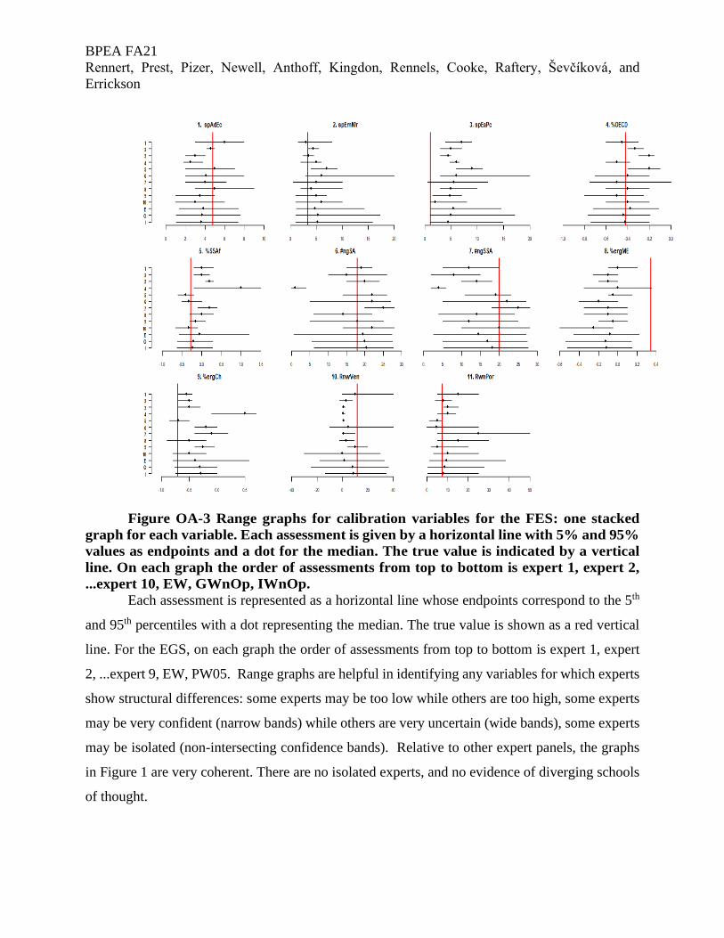
BPEA FA21


Errickson

Figure OA-3 Range graphs for calibration variables for the FES: one stacked

graph for each variable. Each assessment is given by a horizontal line with 5% and 95%

values as endpoints and a dot for the median. The true value is indicated by a vertical

line. On each graph the order of assessments from top to bottom is expert 1, expert 2,

...expert 10, EW, GWnOp, IWnOp.

Each assessment is represented as a horizontal line whose endpoints correspond to the 5th

and 95th percentiles with a dot representing the median. The true value is shown as a red vertical

line. For the EGS, on each graph the order of assessments from top to bottom is expert 1, expert

2, ...expert 9, EW, PW05. Range graphs are helpful in identifying any variables for which experts

show structural differences: some experts may be too low while others are too high, some experts

may be very confident (narrow bands) while others are very uncertain (wide bands), some experts

may be isolated (non-intersecting confidence bands). Relative to other expert panels, the graphs

in Figure 1 are very coherent. There are no isolated experts, and no evidence of diverging schools

of thought.

BPEA FA21


Errickson

6. Conclusion

The expert data presented here is unusual in the number of experts with high statistical

accuracy. Both the equal weight and performance weighted decision makers show good statistical

accuracy with the latter exceeding the informativeness of the former. The results are quite robust

against loss of expert and loss of calibration variable. On the whole the expert group is quite

coherent. When the sociology of expert judgment comes to be written, this example will be a poster

child.

7. References

1. Cooke RM (1991) Experts in Uncertainty-Opinion and Subjective probability in

science. (Oxford University Press).

2. Colson AR & Cooke RM (2017) Cross validation for the classical model of

structured expert judgment. Reliab. Eng. Syst. Saf. 163:109-120.

3. Colson AR & Cooke RM (2018) Expert Elicitation: Using the Classical Model to

Validate Experts' Judgments. Review of Environmental Economics and Policy 12(1):113-132.

4. Eggstaff JW, Mazzuchi TA, & Sarkani S (2014) The effect of the number of seed

variables on the performance of Cooke's classical model. Reliability Engineering & System Safety

121:72-82.

5. Flandoli F, Giorgi E, Aspinall WP, & Neri A (2011) Comparison of a new expert

elicitation model with the Classical Model, equal weights and single experts, using a cross-

validation technique. Reliability Engineering & System Safety 96(10):1292-1310.

6. Cooke, Roger M., Marti, Deniz and Mazzuchi, Thomas A., (2020) Expert

Forecasting with and without Uncertainty Quantification and Weighting: What Do the Data Say?

International Journal of Forecasting, published online July 25 2020

https://doi.org/10.1016/j.ijforecast.2020.06.007

III. Economic Growth Survey: Additional results

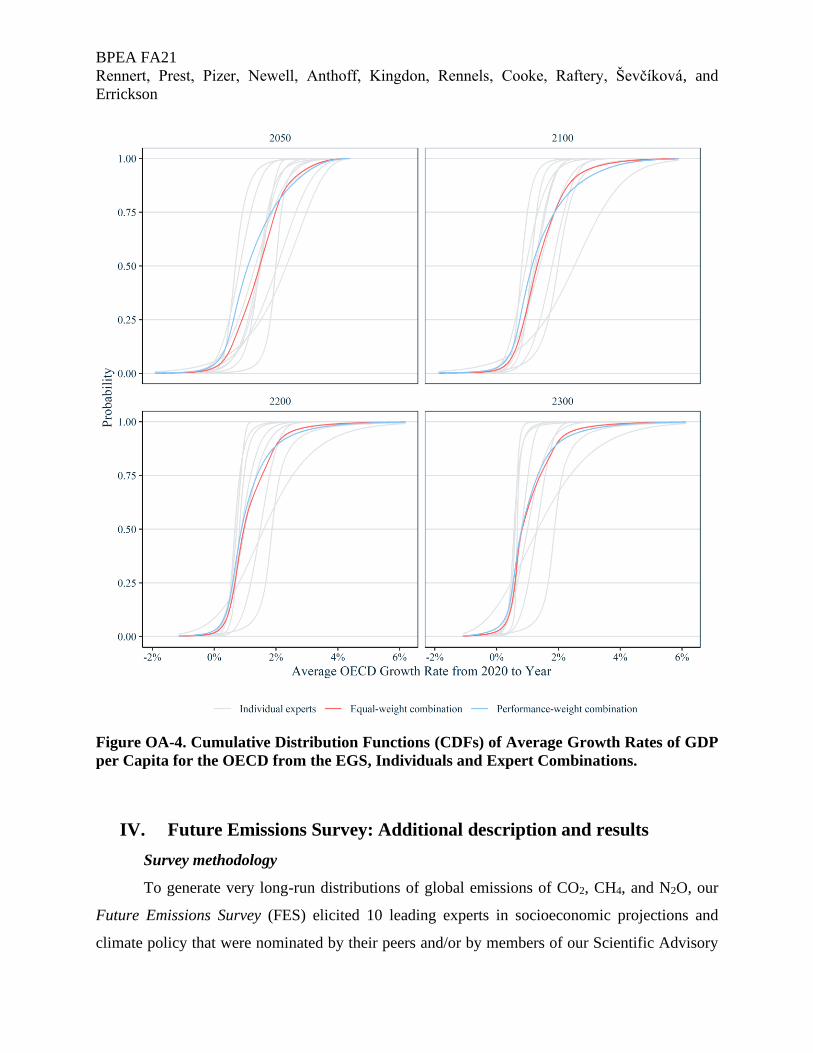
https://doi.org/10.1016/j.ijforecast.2020.06.007

BPEA FA21


Errickson

Figure OA-4. Cumulative Distribution Functions (CDFs) of Average Growth Rates of GDP

per Capita for the OECD from the EGS, Individuals and Expert Combinations.

IV. Future Emissions Survey: Additional description and results

Survey methodology

To generate very long-run distributions of global emissions of CO2, CH4, and N2O, our

Future Emissions Survey (FES) elicited 10 leading experts in socioeconomic projections and

climate policy that were nominated by their peers and/or by members of our Scientific Advisory

BPEA FA21


Errickson

Board. The experts surveyed were based at universities, non-profit research institutions, and

multilateral international organizations. They have expertise in, and have undertaken, long-term

projections of the energy-economic system under a substantial range of climate change mitigation

scenarios.

As with our Economic Growth Survey, the FES employed the Classical Model of structured

expert judgment in which experts first quantified their uncertainty with regard to a set of relevant

calibration variables for which true values are known, for the purposes of validation and

performance weighting in the combining of the expert distributions. Each elicitation was

conducted individually by videoconference in July and August of 2021 in sessions that lasted ~2

hours, and experts provided additional detail as needed by email and videoconference. Experts

participated in the survey in their own capacity and were provided an honorarium where

appropriate.

In the survey, experts provided quantiles of uncertainty (minimum, 5th, 50th, 95th,

maximum, as well as additional percentiles at the expert’s discretion) for four variables for a case

referred to as Evolving Policies, which incorporates views about changes in technology, fuel use,

and other conditions, and consistent with the expert’s views on the evolution of future policy. The

Evolving Policies case corresponds to the USG approach to benefit cost analysis, which evaluates

US regulations as incremental against a more expansive backdrop of other policies and conditions

and is responsive to NASEM recommendations for including future background policy in the

uncertain distributions of socioeconomic projections.

Experts provided quantiles of uncertainty for the following four non-overlapping

categories: (1) fossil and process related CO2 emissions; (2) changes in natural CO2 stocks and

negative emission technologies; (3) CH4; and (4) N2O. They did this for each benchmark year:

2050, 2100, 2150, 2200, and 2300. For the first category, they were also asked to indicate the

sensitivity of emissions to five underlying GDP per capita trajectories. More precisely, they were

asked to provide for each benchmark year:

1) Global CO2 emissions for five levels of future of GDP per capita representing the

minimum, 2.5th percentile, 50th percentile, 97.5th percentile, and maximum of projected

economic growth in each benchmark year (i.e., a separate set of quantiles for each of the

BPEA FA21


Errickson

five GDP per capita levels drawn from the MSW dataset). Reported emissions in this

category included net total emissions from processes, including CCS applied to fossil

energy and process-related emissions. By construction, emissions reported for this

category are greater than or equal to 0.

2) Quantiles of the net CO2 emissions from the combined sum of Agriculture, Forestry, and

Other Land Use (AFOLU) and sequestered emissions from Direct Air Capture (DAC)

and Bioenergy with Carbon Capture and Storage (BECCS). By construction, total net

emissions in this category could be positive (net CO2 source) or negative (net CO2 sink).

3) Quantiles of global CH4 emissions including CH4 emissions from AFOLU.

4) Quantiles of global N2O emissions including N2O emissions from AFOLU.

The categories were designed, and experts were specifically directed, to avoid double

counting of emissions in the distributions provided. Taken together, the elicited source categories

account for greater than95% of current global emissions of greenhouse gases. Experts were

permitted, but not required, to provide quantiles for AFOLU, DAC, BECCS, CH4, and N2O

conditioned on economic growth in the same manner as CO2 emissions in category 1). Experts

were permitted to consult outside sources at their discretion for this section of the survey.

During the survey, experts provided their quantiles by dictating values for their quantiles for each

of the specified categories, years, and economic growth trajectories. The values were recorded in

a spreadsheet visible to the expert during the elicitation via screen share.

Summary of Expert Rationale

As part of FES, experts described their rationale and the conditions supporting their

provided distributions of emissions. The rationale were provided independently, but when viewed

across the full set of experts, featured a number of common and primary factors, including

economic growth, global climate policy ambition and success of implementation, and technology

evolution. Each of these factors could work in concert with or against each other to result in the

final uncertain distribution.

CO2 distributions provided for low economic growth scenarios in general incorporated

divergent potential outcomes. On one hand, low growth was viewed as providing an impediment

BPEA FA21


Errickson

to both policy ambition as well as further improvements in and deployment of low- or zero-

emission energy technologies. On the other hand, low growth was also generally viewed to reduce

global emissions generally as lower economic activity at current or decreased emissions intensity

levels would lead to a decrease in emissions overall. A relatively common narrative supporting the

higher end of emissions distributions was that low economic growth trajectories could lead to a

revisitation of current pledges to reduce emissions and favor continued growth in energy derived

from fossil fuels, leading to further lock-in of such technologies.

For median rates of per capita economic growth, experts in general viewed global policy

as the primary driver, including the success or failure of countries meeting their pledges under the

Paris Agreement and enhancing the ambition of those targets, as well as by the evolution of

developing nations’ use of fossil fuels and assistance provided. Continued evolution of technology,

driven significantly by potential investments consistent with mitigation goals, also featured

prominently as a driver. A common result for the 2050 and 2100 the medians of the emissions

distributions was a reductions of absolute emissions from today’s levels, but with an uncertain

range leaving substantial probability for continued, and in some cases quite significant, increases

as well. The low emission (5th percentile) quantiles generally represented significant reductions

from today’s levels but at a level insufficient keep global temperature increases below 1.5 degrees

Celsius, even when considering reported quantiles for AFOLU.

For high rates of per capita economic growth, several experts expected that significantly

enhanced economic activity would likely lead to increased emissions in the near-term (to 2050 and

for some experts to 2100), as the time needed for further development and deployment of zero-

emission technologies was insufficient to decrease the emissions intensity (emissions/GDP)

quickly enough to offset the economic growth. High economic growth in general was viewed to

support increasing attention to reducing emissions from a policy standpoint and an enhancement

of global climate policy goals, leading to a more rapid medium- and longer-term transition to

greatly reduced emissions overall compared with relatively lower economic growth scenarios. An

alternative viewpoint expressed was that greater wealth could also allow for greater adaptation or

indifference to the effects of climate change, thereby acting as a brake on policy ambition and

allowing for continued increases in emissions well into the future.

BPEA FA21


Errickson

Several experts also observed that, if global policy were to remain largely centered around

absolute quantity targets (e.g., percent reduction from 2005 levels or net zero by a date certain),

emissions would be relatively decoupled from economic growth. Their view of this decoupling

manifested itself in the form of relatively low variation between their distributions across economic

growth trajectories. Similarly, some of the experts felt that the high economic growth trajectories

in particular represented worlds in which economic growth was decoupled from emissions.

Experts generally viewed near-term potential from DAC and BECCS as limited through

2050, but they became an increasing and more substantial part of the solution alongside natural

land sinks by 2100. In general the experts allowed room for the narrative that society may wish to

have net negative annual emissions for several decades even after eliminating direct emissions to

draw down atmospheric CO2 concentrations to return to a level consistent with current or previous

levels.

Emissions from methane are primarily driven by livestock (enteric fermentation),

agriculture (including cultivation of rice), and fossil fuels (natural gas), and experts’ distributions

were primarily driven by their expectations on the future evolution of emissions from these

sources. Experts that viewed a rapid transition to zero-emitting energy sources as relatively likely

tended to have distributions that reflected the rapid zeroing out of the component of CH4 emissions

from fossil fuels. Other experts allowed for the expansion of such emissions in acknowledgement

that natural gas may be relied upon heavily as a transition fuel or even as a significant and

substantially increasing source of uncontrolled emissions over the long-term. In nearly all cases

there was a non-zero lower limit reached, even in the lower quantiles, in acknowledgment that

some components of these emissions were unlikely to be fully eliminated by complete

modification of diet or agricultural practices. Experts’ supporting rationale for N2O, which is

similarly associated with agriculture and dietary preferences, generally followed a narrative

consistent with the corresponding elements from CH4.

During the FES, some experts expressed a desire for further control over the correlations

between variables. The first correlation desired was to condition emissions on population in

addition to GDP per capita. Experts expressing this desire in general agreed with the design

decision to condition on GDP per capita rather than GDP (the product of GDP per capita and

population) as the primary variable and accommodated the study design by providing quantiles

BPEA FA21


Errickson

constructed to incorporate the possibility of low and high population futures. Some experts also

expressed a desire to more tightly couple their quantiles of category 1 emissions with the

potentially negative emissions from category 2 by providing a single distribution of net emissions

from both categories. These experts generally viewed the level of negative emissions as being

tailored to achieve a particular atmospheric CO2 outcome or directly to offset emissions.

Accounting for this correlation would lead to narrower distributions of net emissions overall.

Additional results for CO2 emissions

Figure OA-5: Projected total atmospheric CO2 concentration. Solid lines represent median

values, dark and light shading represent the 5th to 95th (darker) and 1st to 99th (lighter)

percentile ranges based on the RFF-SPs.

BPEA FA21


Errickson

Figure OA- 6: Cumulative distribution functions (CDFs) of individual and combined expert

projections for annual CO2 emissions across a range of timeframes and GDP per capita

growth trajectories.

BPEA FA21


Errickson

Figure

OA-7: Annual net CO2 emissions from natural carbon stocks and negative emissions

technologies

Figure OA-8: Cumulative distribution functions (CDFs) of individual and combined expert

projections for net CO2 emissions from natural carbon stocks and negative emissions

technologies across a range of timeframes

CH4 emissions

BPEA FA21


Errickson

Figure OA-9: Annual emissions of CH4 from the RFF-SPs and the SSPs. Lines represent

median values, and dark and light shading represent the 5th to 95th (darker) and 1st to

99th (lighter) percentile ranges of the RFF-SPs.


projections for annual CH4 emissions across a range of timeframes

N2O emissions

BPEA FA21


Errickson

Figure

OA–11 Annual emissions of N2O from the RFF-SPs and the SSPs. Lines represent median

values, and dark and light shading represent the 5th to 95th (darker) and 1st to 99th (lighter)

percentile ranges of the RFF-SPs.


projections for annual N2O emissions across a range of timeframes

V. Additional SCC calculations

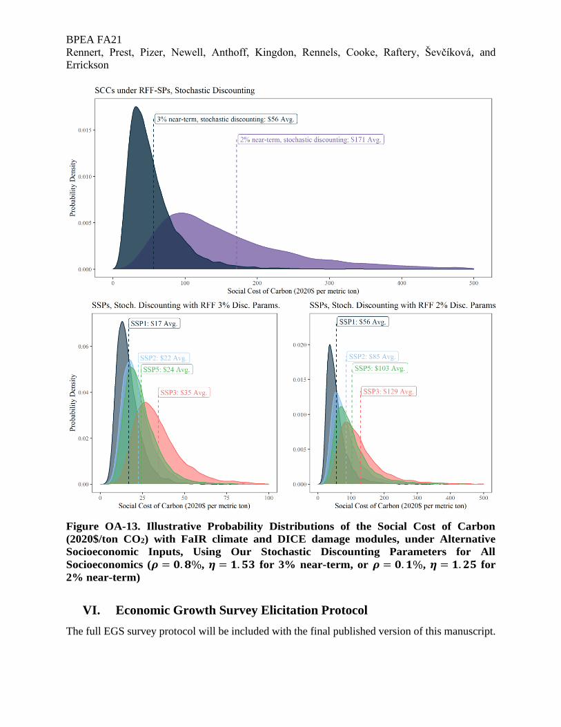
BPEA FA21


Errickson

Figure OA-13. Illustrative Probability Distributions of the Social Cost of Carbon

(2020$/ton CO2) with FaIR climate and DICE damage modules, under Alternative

Socioeconomic Inputs, Using Our Stochastic Discounting Parameters for All

Socioeconomics (𝝆 = 𝟎. 𝟖%, 𝜼 = 𝟏. 𝟓𝟑 for 3% near-term, or 𝝆 = 𝟎. 𝟏%, 𝜼 = 𝟏. 𝟐𝟓 for

2% near-term)

VI. Economic Growth Survey Elicitation Protocol

The full EGS survey protocol will be included with the final published version of this manuscript.

BPEA FA21


Errickson

VII. Future Emissions Survey Elicitation Protocol

The full FES survey protocol will be included with the final published version of this manuscript.

Documents

The Social Cost of Carbon: Advances in Long-Term