Embed Size (px)
Citation preview
The Single Layer Heat Potential andGalerkin Boundary Element Methods for
the Heat Equation
byPatrick James Noon
Dissertation submitted to the Faculty of the Graduate Schoolof The University of Maryland in partial ful�llment
of the requirements for the degree ofDoctor of Philosophy
����
Advisory Committee�Professor D� N� ArnoldProfessor I� BabuskaProfessor R� B� KellogProfessor F� W� J� OlverProfessor J� R� Dorfman

Contents
� Introduction �
� The Anisotropic Sobolev Spaces� Trace Theory �
��� Preliminaries and the Time Restriction Operator � � � � � � � ���� De�nition of the Trace Operator � � � � � � � � � � � � � � � � � ����� Mapping Properties of the Trace Operator � � � � � � � � � � � ��
� Mapping Properties of the Heat Operator ��
� Mapping Properties of the Single Layer Heat Potential ��
� Regularity of the Single Layer Operator ��
�� Boundedness � � � � � � � � � � � � � � � � � � � � � � � � � � � ���� Surjectivity � � � � � � � � � � � � � � � � � � � � � � � � � � � � �
� Galerkin Discretization of the First Kind Boundary Integral
Equation �
�� Construction of the Trial Space � � � � � � � � � � � � � � � � � ��� Implementation � � � � � � � � � � � � � � � � � � � � � � � � � � ��� Application to the Direct Integral Equation � � � � � � � � � � ��� Higher Order Methods in Time � � � � � � � � � � � � � � � � � �
Error Analysis of the Galerkin Method ��
��� Approximation Theory in the Anisotropic Sobolev Spaces � � � ���� Error Estimates I � � � � � � � � � � � � � � � � � � � � � � � � � ���� The Aubin Nitsche Lemma and Interior Error Estimates � � � ���� Error Estimates II � � � � � � � � � � � � � � � � � � � � � � � � ��
� Numerical Examples
A Proof of Theorem ��� ��
B Proof of Theorem �� ��
C Solutions to the Heat Equation Over the Unit Circle ��
ii

Abstract
Title of Dissertation� The Single Layer Heat Potential and GalerkinBoundary Element Methods for the Heat Equation
Patrick James Noon� Doctor of Philosophy� �����
Dissertation directed by� Douglas N� Arnold� Associate Professor� AppliedMathematics Department�
We study Galerkin boundary element discretizations of the single layer heatpotential operator equation
K�q ��Z t
�
Z�K�x� y� t� t��q�y� t��dydt� � F �x� t�� x � �� t � �� �����
where K denotes the fundamental solution
K�x� t� �
�����
exp��jxj���t����t����
x � R�� t � �
� x � R�� t � ��
We �rst formulate a well posedness theory for ����� and show that for eachF in the anisotropic Sobolev space H����������R��� there exists a uniquesolution q in its dual space H������������R�� which depends continuouslyon the data in the sense that
kqkH������������R�� � ckFkH����������R���
Moreover� we show that K� satis�es a coercivity estimate
Re hq�K�qi � ckqk�H������������R���
We next develop a regularity theory for the mapping K� and show that K�
�in the scale of anisotropic Sobolev spaces Hr�s���R�� for r� s � �� may beregarded as an operator which increases regularity by one spatial derivativeand one half time derivative� These results provide a basis for oursubsequent analysis of a class of Galerkin discretizations methods based ontest and trial spaces of piecewise polynomials� We show optimalconvergence in the energy norm H������������R�� and investigate the rateof convergence in L����R��� Finally� to test our conclusions� we presentnumerical examples�

� Introduction
The classical method of boundary integral equations uses speci�cally de �ned solutions called layered potentials and reduces the given boundary valueproblem into an integral equation of the second kind� Thus� a double layerpotential is used to treat Dirichlet problems� whereas a single layer poten tial is used to solve Neumann problems� The overwhelming reason for theseselections is the well known results on the unique solvability of second kindintegral equations� Besides being well posed in a variety of spaces� secondkind integral equations are often well suited� �in regards to both implemen tation and analysis�� to various approximate methods such as Galerkin orcollocation type methods�
Although the layered potential approach is more commonly associatedwith elliptic problems� it also has a long history in the study of parabolicboundary value problems� Holmgren ���� initially introduced the heat po tentials in two variables �i�e�� one time and one space variable� and usedthem to show the solvability of the heat equation� Gevrey ���� subsequentlyextended the argument to more general parabolic problems of two variables�Generalizations to problems in several space dimensions were slow to appearsince the kernel of the second kind Volterra integral equation which arises wasnot fully understood� Pogorzelski ��� �� ��� ��� showed the basic solvabil ity of this integral equation in arbitrarily many space dimension on smoothmanifolds� His arguments helped to establish the basic well posedness of awide variety of parabolic problems�
Currently� the application of boundary element methods to parabolicproblems is being actively considered� Essentially� boundary element meth ods refer to numerical solutions of the integral equations encountered in thelayered potential method� In contrast to the classical approach� however�the integral equation typically used for numerical purposes is the so calleddirect integral equation of heat conduction� In the case of problems withDirichlet boundary conditions� this equation results in a �rst kind Volterraintegral equation� Though this approach is often used in practice ���� ��������� ����� ����� the basic convergence theory behind it has yet to be given�In this paper� we analyze the direct integral equation method applied to aninitial Dirichlet boundary value problem for the heat equation�
We start by recalling the direct integral equation� Let u�x� t� solve the
�
initial Dirichlet boundary value problem
�u
�t�x� t���u�x� t� � �� x � �� t � �� �����
u�x� �� � f�x�� x � �� �����
u�x� t� � g�x� t�� x � �� t � �� �����
where � denotes a bounded� open set in R�� Set K�x� t� equal to the funda mental solution to the heat equation� i�e��
K�x� t� �
�����
exp��jxj���t����t����
x � R�� t � �
� x � R�� t � ��
Then� a simple application of Green�s theorem �see ���� pp� ������� showsthat the solution u to ��������� must satisfy the integral equation
u�x� t� �Z t
�
Z�
�K�x� y� t� t��
�u
�ny�y� t��� �K
�ny�x� y� t� t��g�y� t��
�dydt�
�ZK�x� x�� t�f�x��dx�� x � �� t � �� �����
where � denotes the boundary of � and ny the unit outward normal derivativeto � at y� We will assume that � is a smooth C� surface� Observe how thedirect integral equation ����� relates u throughout � �R� to its initial andboundary data�
The �rst term of ������ �where we have set q � �u��ny�
U��x� t� ��Z t
�
Z�K�x� y� t� t��q�y� t��dydt�� x � R�n�� t � �� ����
is called the single layer heat potential with density q� Similarly� the secondterm of �����
U��x� t� ��Z t
�
Z�
�K
�ny�x� y� t� t��g�y� t�dydt�� x � R�n�� t � � ����
is the double layer heat potential with density g� Assuming that q and gare continuous on ��R�� each of these potentials de�nes a C� function onx � R
�n� and t � � which satisfy the heat equation there and vanish for
�

t � �� They also satisfy jump conditions �cf�� ���� p� ����� similar to thosesatis�ed by the corresponding single and double layer electrostatic potentials�As x� � R�n� tends non tangentially to x � �� we have
limx��x
U��x�� t� � U��x� t�� �����
limx��x
�U�
�nx�x�� t� � ��
�q�x� t� �
Z t
�
Z�
�K
�nx�x� y� t� t��q�y� t��dydt�� �����
limx��x
U��x�� t� � ��
�g�x� t� �
Z t
�
Z�
�K
�ny�x� y� t� t��g�y� t��dydt�� �����
In these equations� the upper sign holds when the limit is approached fromthe interior while the lower sign holds when the limit is approached from theexterior�
Letting x in ����� tend to the boundary �� the jump conditions yield theboundary integral equation
�
�g�x� t� �
Z t
�
Z��K�x� x�� t� t��q�x�� t��� �K
�ny�x� y� t� t��g�y� t���dydt�
�ZK�x� x�� t�f�x��dx�� x � �� t � �� ������
This is a �rst kind Volterra integral equation for the unknown Neumann dataq � �u��n of the form
K�q ��Z t
�
Z�K�x� y� t� t��q�y� t��dydt� � F �x� t�� x � �� t � �� ������
where
F �x� t� ��
�g�x� t� �
Z t
�
Z�
�K
�ny�x� y� t� t��g�y� t��dydt�
�ZK�x� x�� t�f�x��dx�� �x� t� � � �R��
Conversely� if we were studying the Neumann �or Robin� boundary valueproblem� ����� would result in a second kind Volterra integral equation forthe unknown Dirichlet data u� For example� the form of this equation forthe Neumann problem would be
�
�u�x� t� �K�u�x� t� � F �x� t�� x � �� t � � ������
�

where F �x� t� is known and where K� denotes the integral operator
K�p�x� t� �Z t
�
Z�
�K
�ny�x� y� t� t��p�y� t��dydt�� x � �� t � �� ������
The theory of ������ is well developed� Assuming that � is a C� surface�Pogorzelski ��� showed that the kernel of ������ satis�es the estimate
j �K�ny
�x� t�j � C�t��jxj�n��� for all � � ����� ��� ������
and is therefore weakly singular� From ������� it follows that K� has normless than � on C��� ��� T �� for T su�ciently small� Thus� I �K� is invert ible for su�ciently small T � Since K� is of convolution type� however� theexistence of �I � K���� on C�� � ��� T �� for any �nite value of T is easy toshow by successively considering I � K� over subintervals of small length�The same reasoning applies to I � K� on L��� � ��� T ��� In ����� Pogorzel ski showed that K� de�nes a compact mapping on the space of continuousfunctions� The compactness of the operator K� is relevant to the study ofnumerical discretizations� In particular� the convergence of a broad class ofmethods known as projection methods �which include Galerkin and colloca tion methods� is assured when applied to operators of the form I � K withK compact� More recent treatments of ������ have focused on the case ofunsmooth boundaries� Though K� no longer remains compact� the basic solv ability of this equation holds in a wide variety of function spaces� For moredetails� see ����� ����� A treatment of the numerical solution of this equationhas been given in some generality by Costabel� Wendland and Onishi �����
The theory of equation ������� however� is less straightforward then thatof ������� Indeed� until the recent work of Brown ���� even the basic wellposedness of this equation had not been addressed� Our �rst goal is to es tablish the well posedness of ������ in such a way to provide a basis for thesubsequent analysis of discretizations� We do this by giving a variationalinterpretation of ������� extending to the parabolic setting the argument ofNedelec and Planchard ���� who treated the electrostatic single layer poten tial in this fashion� The main advantage of this viewpoint is that Galerkindiscretizations methods may then be analyzed by standard techniques�
To explain our results� we brie�y summarize the argument in ����� LetW ��R�� denote the closure of D�R�� in the norm
k�kW ��R�� � kr�kL��R��� � � D�R���
�

The inner product
�u� v�W ��R�� �ZR�ru�x�rv�x�dx� �����
induces a Hilbert space structure on W ��R��� Even though W ��R�� is notincluded in L��R��� we have the dense inclusions
D�R�� � H��R�� � W ��R���
Consequently� the dual �W ��R���� of W �R�� is identi�able with a subset ofdistributions strictly contained in H���R��� As is customary� we denote thisspace by W���R���
The space W ��R�� is introduced because the natural isomorphism fromW ��R�� onto W���R�� de�ned by the inner product ����� clearly extendsthe distributional de�nition of the �negative� Laplacian operator ��� Thisexplains why the space W ��R�� has been well studied� Based on Sobolev�sinequality �����
kkL��R�� � CkrkL��R��� for all � D�R���
it follows that W ��R�� is identical �algebraically and topologically� to thesubset of L�R�� functions whose gradients belong to L��R��� Moreover� theweighted L� estimate�
ZR�jxj��ju�x�j�dx � Ckruk�L��R��� u � W ��R��� �����
shown by Hardy�s inequality� shows that W ��R�� is a space of locally inte grable functions which di�ers from the space H��R�� solely in its permittedbehavior at in�nity� Consequently� the trace operator of restriction fromR� to � extends to a surjection of W ��R�� onto H������� These facts enable
one to show that the operator K � � ������ � � de�nes an isomorphismof H������� onto H������� It remained for Nedelec and Planchard to showthat K extends the classical single layer potential
Kq�x� � �
��
Z�
q�y� dy
jx� yj � x � R�� q � D�R���

For our treatment� it will be necessary to work in the setting of theanisotropic Sobolev spaces �cf�� ��� Chapter �� �� For all non negative realnumbers r and s� we use Hr�s to denote the Hilbert spaces
Hr�s � L��R�Hr�R��� Hs�R� L��R����
with associated norm
kuk�Hr�s � kuk�L��R�Hr�R��� � kuk�Hs�R�L��R����
Analogously� let Hr�s���R�� denote the Hilbert space
Hr�s���R�� � L��R��Hr���� Hs�R�� L
������ ������
withkuk�Hr�s���R��
� kuk�L��R��Hr���� � kuk�Hs�R��L������
The utility of these anisotropic Sobolev spaces in treating the heat equa tion is evident in the discussion in ��� Chapter �� and the recent work of��� Accordingly� there is a well developed theory of the trace operator onthese spaces� Letting � denote an extension of the restriction operator fromfunctions on R��R to functions on ��R�� the results in ��� Theorem ����p� ��� imply that � extends to a bounded� linear operator of Hr�s ontoHr������r�����s�r���R�� for all r � ��� and any s � �� We give a completereview of this trace theorem in section � since we also require an importantadditional trace result which shows that � even maps the smaller Sobolevspace
V � fu�x� t� � L��R�H��R�����u
�t�x� t� � L��R�H���R���g�
onto H����������R���In section �� we de�ne spaces of functions over R� �R which are analo
gous to the space W ��R�� and establish the mapping properties of the heatoperator on them� In section � we prove a major result of this paper� Weshow that the single layer heat potential operator K� extends from smoothfunctions to an isomorphism of H������������R�� isomorphically onto its dualH����������R��� Furthermore� we show that K� satis�es the coercivity esti mate
hq�K�qi � ckqk�H������������R���

It is remarkable that the single layer heat potential satis�es such a coer civity estimate� This kind of estimate is more typical of elliptic operatorsand it does not hold for the heat operator� Besides being of theoretical in terest� this coercivity has immediate applications to the study of Galerkindiscretization methods which are known to be quasioptimal when applied tocoercive operators�
Before discussing the Galerkin methods� we consider the regularity of themapping K�� Letting �s � R��
Xs�����R�� � fu � H�s�s���R�� � U � H�s�s such that
U � u �a�e� t � �� U � � �a�e� t � �g�
we show that K�� Xr�������� ���R�� � X
r�������� ���R�� is an isomorphism
for all non negative r� The case r � ��� of these results agrees with theresults of R� Brown ��� who showed �by very di�erent methods� that K� isan isomorphism of L��� � R�� onto H��������R�� for any Lipschitz surface�� This discussion is contained in section �
In section and section �� we discuss the implementation and error anal ysis for a Galerkin discretization of ������� We study the Galerkin methodsince a complete error analysis for the method may be given� The error anal ysis shows that if the di�erent mesh sizes in time and space concurrentlydecrease in a appropriate way� the Galerkin method converges with optimalorder in L����R��� To test this and other claims� we present some numericalexamples in section ��
�

� The Anisotropic Sobolev Spaces� Trace
Theory
In this section� we review the de�nition and theory of the anisotropic Sobolevspaces� In section ���� we recall the de�nitions of the spaces over R��R� Theremaining sections focus on the mapping properties of the trace operator�
��� Preliminaries and the Time Restriction Operator
As noted in the introduction� the anisotropic Sobolev spaces Hr�s are de�nedfor all r� s � � by
Hr�s � L��R�Hr�R��� Hs�R� L��R����
Norms over Hr�s may be de�ned using Fourier transforms in space and time�We will denote this operator by Fx�t and will assume that it is de�ned onsmooth functions u � S�R� �R� by
Fx�t�u� �Z �
��
ZR�u�x� t�e�ix�e�it�dxdt� ��� � � � R� �R�
and extended to S ��R� �R� by Parseval�s theorem� In terms of the Fouriertransform� an equivalent norm on Hr�s is given by
kuk�Hr�s �Z �
��
ZR�
h�� � j�j��r � �� � j� j��s
ijFx�t �u� ��� � �j�d�d�� �����
The continuous inclusions
D�R� �R� � L��R� �R�� � Hr��s� � Hr��s� � � � r� � r�� � � s� � s��
are dense� Once and for all� we note the existence of positive constants cr�sand Cr�s such that
cr�s�� � j�j�r � j� j�s� �n�� � j�j��r � �� � j� j��s
o� Cr�s�� � j�j�r � j� j�s��
for all r� s � ��In this paper� it will be convenient to consider the spaces Hr�s as being
complex valued� Thus� the appropriate de�nition of the spaces H�r��s is as
�
the antidual space to Hr�s� That is� the space of continuous� antilinear forms��An antilinear form means a mapping f � Hr�s � C which satis�es
f� �u� � �u�� � �f�u�� � �f�u��� u�� u� � Hr�s� �� � � C ��
It is not hard to show that the spaces H�r��s so obtained are equivalent tothe sum space
H�r�s � L��R�H�r�R��� �H�s�R� L��R����
with the sum norm
kfk� � inff�f��f�
�kf�k�L��R�H���R�� � kf�k�H�����R�L��R���
�� f � H�r��s�
They are also equivalent to the set of locally integrable functions f for which
f ��Z �
��
ZR�
jFx�t�f���� � �j��� � j�j� j� js�r��rd�d�
���
�
is �nite�With r � � arbitrarily �xed and s � ��� ��� an equivalent norm on Hr�s is
given by
kuk�Hr�s �Z �
��ku��� t�k�Hr�R��dt�
Z �
��
Z �
��
ku��� t�� u��� t��k�L��R��
jt� t�j���s dtdt�� �����
For larger values of s� let m equal the integer part of s and set � � s �m�Then� the expression
kuk�Hr�s � kuk�Hr�� � ku�m�k�Hr�� � �����
de�nes an equivalent norm on Hr�s� Based on ���������� a natural de�nitionof the spaces Hr�s�R��R�� for s � ��� �� is made using the norm
kuk�Hr�s�R��R���
Z �
�ku��� t�k�Hr�R��dt
�Z �
�
Z �
�
ku�m���� t�� u�m���� t��k�L��R��
jt� t�j���� dtdt��
�

Similarly� for higher values of s� one can de�ne the spaces Hr�s�R��R� by thenorms
kuk�Hr�s�R� �R��� kuk�Hr���R��R��
� ku�m�k�Hr���R��R��
Using ���������� it is simple to check that the restriction of U � Hr�s tothe set R� � R� belongs to Hr�s�R��R�� for any r� s � �� It is well knownthat this restriction operator actually maps Hr�s�R��R� onto Hr�s�R��R��for all r� s � �� This follows from the existence of an extension operatorwhich simultaneously extends Hr�s�R��R�� to Hr�s for all r� s � �� For manypurposes� such as ours� this weaker result su�ces�
Lemma ��� For each positive integer M � there exists an extension operatorEM which depends on M such that
EM �Hr�s�R��R��� Hr�s for all s � ���M �� any r � ��
with EMu�x� t� � u�x� t� for almost all �x� t� � R� �R��
Remark� A standard choice for EM is the operator
EMu�x� t� �
u�x� t�� x � R�� t � ��Pm
j�� �ju�x��jt�� x � R�� t � ��
where the coe�cients �j are chosen to satisfy
mXj��
��j�k�j � � � � k � m� ��
There are two important subspaces of Hr�s�R��R�� we will need to use�One is the subspace Hr�s
� �R��R�� which is de�ned as the closure of D�R��R��in the Hr�s�R��R�� norm� For all s � ���� this is a strictly proper sub space of Hr�s�R��R��� For s � ��� ����� however� this space coincides withHr�s�R��R��� �The case s � ��� is a non trivial result which is proven in������
The other subspace we need is the space Hr�s�� �R
��R��� This space isde�ned to be the space of functions u such that there exists some functionU � Hr�s�R��R� which agrees with u for all t � � and vanishes for all t � ��It is a Hilbert space when given the norm
kukHr�s�R��R�� � infUkUkHr�s�
��

where the in�mum is taken over all such U �s� Although the de�nition of thisspace is di�erent than the de�nition of the space Hr�s
� �R��R��� it turns outthat these two spaces coincide for all r� s � � except for the s values whichsatisfy s � m � ��� with m � N� For these special values of s� the space
Hr�m������ �R��R�� is a strictly proper subspace of Hr�m����
� �R��R���
Remark� It is customary to de�ne the spaces Hr�s�� �R
��R�� only for s� ��� �N� since they agree with Hr�s
� �R��R�� otherwise� In this paper� however� itis natural to de�ne Hr�s
�� for all r� s � � since they are the proper setting forthe regularity theory in section �
The negative indexed Sobolev spaces H�r��s�R��R�� are de�ned as theantidual spaces to Hr�s
� �R��R�� with corresponding norm
kqkH�r��s�R��R�� � supg�Hr�s
� ���R��
hq� gikgkHr�s���R��
�
Again� these spaces can be shown to be equivalent to the sum spaces
H�r�s � L��R��H�r�R��� �H�s�R�� L
��R����
with the sum norm
kfk� � inff�f��f�
�kf�k�L��R��H�r�R�� � kf�k�H�s�R��L��R���
��
It is important to note that H�r��s���R�� is not the antidual space ofHr�s�R��R�� for all s � ����
Clearly� the spaces Hr�s�R��R�� and Hr�s�� �R
��R�� are intimately con nected with the time restriction operator R� and the zero extension operatorZ�� �That is�
Z�u�x� t� �
u�x� t�� x � R�� t � ��
�� x � R�� t � ��
By de�nition� each of the mappings R�� Hr�s � Hr�s�R��R�� and Z��Hr�s
�� ���R�� � Hr�s are bounded for all r� s � �� Both of these operatorscan be extended into the dual spaces� To extend Z�� consider the adjointmapping R��� �Hr�s�R��R���� � H�r��s� For all f � H�r��s� this map isde�ned by
hR��f� Ui � hf�R��Ui for all U � Hr�s�
��

Thus� for f � L��R� �R�� we have
hR��f� Ui �Z �
�
ZR�f�x� t�U�x� t�dxdt� for all U � Hr�s�
which agrees with the zero extension of f � Analogously� the adjoint operatorZ�� extends the restriction operator R�� The equality of Hr�s
� �R��R�� withHr�s
�� �R��R�� for all r� s � � such that s� ��� �� N shows that R�� H�r��s �
Hr�s�R��R�� is bounded for these values� For easy reference� we summarizethe mapping properties of these operators in a lemma�
Lemma ��� Let R�� D�R� � R� � C��R� � R�� denote the restrictionoperator in time� Then� R� extends to a bounded linear mappings of
Hr�s�R��R�� Hr�s�R��R�� for all r� s � ��
H�r��s�R��R�� H�r��s�R��R�� for all r� s � �� such that s� ��� �� N�Analogously� let Z�� D�R� � R�� � D�R� � R� denote the operator of ex�tension by zero to t � �� Then� Z� extends to a bounded linear mappingof
Hr�s�� �R
��R��� Hr�s� for all r� s � ��
We will also use anisotropic Sobolev spaces de�ned over other spatialregions besides R�� For any r� s � � and any open set O � R�� the spacesHr�s�O�R� can be de�ned as the space of restrictions to O �R of Hr�s� Thecorresponding norm of this space is
kukHr�s�O�R� � inf kUkHr�s �
where the in�mum is taken over all U � Hr�s which agree with u on O �R�Equivalently� these are the spaces
Hr�s�O�R� � L��R�Hr�O�� Hs�R� L��O���
In this paper� the set O shall either be a bounded set in R�� which weshall denote by �� or the complement of such a set� which we will denote by�c� In addition to Hr�s�O�R�� we introduce the space Hr�s
� �O �R� which isde�ned as the closure of D�O�R� in the Hr�s�O�R� norm� Many propertiesare known about both of these spaces� For example� we have
Hr�s� �O �R� � Hr�s�O �R�� � � r� s � ����
��
with Hr�s� �� � R� strictly included in Hr�s�O � R� otherwise� A complete
discussion of these spaces can be found in ��� Chapter ��� For our purposes�it will be su�cient to simply state what else we need at the appropriate time�
��

��� De�nition of the Trace Operator
In the next two sections� we will discuss the theory of the trace operator onthe anisotropic Sobolev spaces� The trace operator considers an extensionof the restriction operator from functions on R� � R to functions on � �R�Although this operator is well understood ��� Chapter ��� we will present itstheory in detail� Mostly� this is because we need to develop some facts whichare not discussed in ���� In this section� we describe the way in which thetrace operator is de�ned through regularization and localization�
To simplify the exposition� we assume throughout that � refers to abounded� open set in R� whose boundary � is an in�nitely di�erentiablemanifold of dimension two and that � lies to one side of �� This stringentassumption on the smoothness of � allows us to discuss the trace mappingon the spaces Hr�s�R��R� for all positive values of r� The weaker assumptionthat � is a Ck�� surface for integer k � � would su�ce to discuss the tracemapping for all r � k� Even this assumption on � could be weakened� butwe will not discuss this matter here� Throughout this section� r and s denotenon negative real numbers with r � ���� We set
� r � ��� and � �s
r�r � �����
The smoothness assumptions on � imply that there exists a �nite coveringof �� by bounded� open sets O� thru OM such that for each integer j between� and M � there is a C� di�eomorphisms �j mapping
Oj onto Y � f�y�� y�� y��� jyij � �� i � �� �� �g�Oj � onto Y� � f�y�� y�� y��� jyij � �� i � �� �� � � y� � �g�Oj � onto Y� � fy � Y � y� � �g�
Furthermore� there exists an open subset O� with closure contained in � suchthat the sets O�� O�� � � � � OM cover of ��� For each j� we let �j equal the inversemappings of �j and for notational convenience introduce the operators
��j �w� �x� t� � w��j�x�� t� w � Hr�s�Y�R�� �����
��j �u� �y� t� � u��j�y�� t�� u � Hr�s�Oj �R�� ����
We have
k��j �w�kHr�s�Oj�R� � C���kwkHr�s�Y�R�� ����
k��j�u�kHr�s�Y�R� � C���kukHr�s�Oj�R�� �����
��
We now introduce a partition of unity subordinate to this covering of�� That is� for each j between � and M � we let �j�x� � D�R�� denote anon negative function which is supported in Oj such that
MXj��
�j�x� � �� x � ��
Details on the construction of these functions may be found in ��� pp� �� ���� Since we will need it shortly� we point out here that we can assume
without loss of generality that the square root ����j of each of these functionsalso belongs to D�Oj�� � If not� we de�ne a new class of functions as thesquares of the original ones and then normalize them�� We then set
�M���x� � � �MXj��
�j�x�� x � R��
to arrive at a partition of unity f�jgM��j�� of R�� Using these functions� we
can write any u � Hr�s�R��R� as
u�x� t� �M��Xj��
�j�x�u�x� t�� �x� t� � R� �R� �����
Note that the x support of �M���x�u�x� t� is disjoint from �� while the xsupport of ���x�u�x� t� has closure contained in �� Thus� these two functionsvanish in a x neighborhood of �� Introducing the maps ��j and ��j into �����leads to the equality
u�x� t� � ���x�u�x� t� �MXj��
��j���j ��ju�
��x� t�
� �M���x�u�x� t�� �x� t� � R� �R� �����
Equation ����� is the basis of localization� To formalize this process� letW denote the product Hilbert space
W � Hr�s� ���R��
MYj��
Hr��Y�R��Hr�s
� ��c�R��
�
with associated norm
k�wk�W � kw�k�Hr�s��R� �MXj��
kwjk�Hr�s�Y�R�
� kwM��k�Hr�s�c�R�� �w�� w�� � � � � wM��� � W�
Now� de�ne T � Hr�s�R��R� to W by
Tu � ���u� ������u�� � � � � �
�M ��Mu�� �M��u� � ������
Clearly� T maps Hr�s�R��R� boundedly into W � A left inverse to T is givenby the mapping
��w�� w�� � � � � wM��� � w��x� t� �MXj��
��j �wj��x� t�
� wM���x� t�� �x� t� � R� �R�Since
kukHr�s�R��R� � k�TukHr�s�R��R� � C���kTukW � ������
T de�nes an isomorphism between Hr�s�R��R� and its range R�T � which isa closed subspace of W � Note that � is not a right inverse of T �
Of course� before the trace map can be de�ned� we must de�ne the Sobolevspaces Hr�s���R�� For each integer j between � and M � we let Oj � Oj ��and set
��j�x� � �j�x�� x � Oj�
Note that O�� O�� � � �� OM cover � and that ���� � � �� ��M are a partition ofunity subordinate to this cover� Again� we introduce the operators
��j �g� �x� t� � g��j�x�� t�� g � D�Y� �R����j �v� �y� t� � v��j�y�� t�� v � D�Oj �R��
The product mapping T � de�ned by
T �v ���������v�� � � � � ��
�M���Mv�
�embeds smooth functions v into a product space� say G� of functions whichare de�ned over R� �R� The mapping �� given by
� ��g�� g�� � � � � gM� �MXj��
��j �gj� �x� t�� �x� t� � � �R�
�

is a left inverse of T �� The norm
kvk�Hr�s���R� �MXj��
k��j���jv�k�Hr�s�R��R��
induces a Hilbert space structure on functions de�ned over ��R� It is wellknown �see ���� Chapter ��� that all choices of covering sets and partitionsof unity lead to equivalent norms�
LetR� denote the operator of restriction from functions de�ned on �y�� y�� t� �R� �R to ones de�ned on �y�� t� � R� �R� We also view R� as an operator
from W to G by
R��w�� w�� w�� � � � � wM��� � �R�w�� R�w�� � � � � R�wM ��
The trace operator is then de�ned for u � Hr�s�R��R� by
u � ��R�Tu�
By construction� agrees with the restriction operator when appliedto smooth functions� Given that the operator R� maps Hr�s�R��R� intoH����R��R�� it follows by de�nition that maps Hr�s�R��R� into H������R��Similarly� if R� maps Hr�s�R��R� onto H����R��R�� then maps Hr�s�R��R�onto H������R�� We elaborate on this and show how to extend a givenv � H������R�� u � Hr�s�R��R� such that u � v�
Let v � H������R� be given and assume that E is a right inverse to R��
Then� by de�nition� the function ��m���mv
��y� t� belongs to H����R��R� for
each integer m between � and M � Using the extension operator E� considerthe following function in Hr�s�R��R��
um�x� t� � ��jh��m��
���m �E
���m
������m v
��i�x� t�� �x� t� � R� �R� ������
Expanding this de�nition out� one can check that um � Hr�s�R��R� and hasx support in Om �R� Its trace on � is
um�x� t� � ��m�x��x�v�x� t�� �x� t� � ��R�Using the linearity of the trace operator and the fact that the functions ��m�x�are a partition of unity with respect to �� it follows that the function
u�x� t� �MXm��
um�x� t�� �x� t� � R� �R
��

belongs to Hr�s�R��R� and satis�es u � v�
Remark� Higher order trace operators �k� for integer values of k are de�nedby
�k�u � ��R��k
�yk�Tu� k �Z��
where one views ���y� as the operator from W to G de�ned by
�
�y��w�� � � � � wM � wM��� � �
�w�
�y�� � � � �
�wM
�y�� ��
These operators extend the classical de�nition of the derivatives �ku��knwith respect to the surface normal direction n�
��� Mapping Properties of the Trace Operator
The discussion in section ��� shows how the properties of the trace operatormay be reduced to studying the restriction operator R� which maps functionsw�y�� y�� t� de�ned on
fy � �y�� y�� � R�� y� � R�� y� � Rg�to functions w�y�� �� t� de�ned on
fy � �y�� �� � R�� y� � Rn��g�Throughout this subsection� we write y � R� as y � �y�� y�� where y� � R�
and y� � R� We shall use � � ���� ��� to denote the corresponding Fouriertransform variables to �y�� y��� We set
� r � ��� and � �s
r �
Theorem ��� The operator R� maps Hr�s�R���R� onto H����R��R� for all
r � ���� s � �� Hence� the trace operator maps Hr�s�R��R�� ontoH������R���
Proof� It su�ces to prove the claim about R�� Let �w���� ��� � � denote theFourier transform of w� The basic relationship between w and its traces isgiven by
Fy��t �w� ���� � � �
Z �
���w���� ��� � �d��� ������
��

Taking absolute values in ������ and applying the Cauchy Schwartz inequal ity� we get
jFy��t �w� ���� � �j� �
�Z �
��d��
k���� ��� � �
�Z �
��k���� ��� � �j �w���� ��� � �j�d��
��
������where
k���� ��� � � � � � j��j�r � j��j�r � j� j�s�To bound the �rst integral of ������� we change variables of integration
by letting �� � �� � j��j�r � j� j�s����r�� We �nd that
Z �
��d��
k���� ��� � ���� � j��j�r � j� j�s
����r Z �
��d�
� � ��r�
Since �r � �� the integral over � is �nite and thus ������ becomes the in equality
�� � j��j�r � j� j�s
���r jFy��t �w� ���� � �j� � C
Z �
��k���� ��� � �j �w���� ��� � �j�d���
Recalling the de�nition of �� it follows by rede�ning the constant C that
�� � j��j�� � j� j��
�jFy��t �w� ��
�� � �j� � CZ �
��k���� ��� � �j �w���� ��� � �j�d���
Integrating this inequality over �� and � and noting that
Z �
��
ZR�
Z �
��k���� ��� � �j �w���� ��� � �j�d��d��d� � C�r� s�kwk�Hr�s� w � Hr�s�
we getkwkH����R��R� � C�r� s�kwkHr�s�R��R�� �����
Equation ����� shows that extends to bounded� linear mapping ofHr�s�R��R� into H����R��R�� To show that it maps onto H����R��R�� weconstruct an extension mapping� Let ���� � D�R� be a non negative functionwhich satis�es Z �
������d� � ��
��

Given g � H����Rn���R�� let �g equal its Fourier transform in space and time�Now� de�ne U by
�U �� Fy��y��t �U� ���� ��� � � ��g���� � �W ���� � �
�����W ���� � ��� �����
whereW ���� � � �
�� � j��j� j� js�r
��
Since� � j�j�r � j� j�s � Cr�s
h�W ��� � ���r � j��j�r
i�
a simple calculation shows thatZ �
���� � j�j�r � j� j�s�j �U��� � �j�d�� � Cj�g���� � �j� �W ���� � ���r��� ������
Integrating ������ over ���� � �� we get
kUkHr�s�R��R� � Cr�skgkH������R��
Since Z �
��U���� ��� � �d�� � �g���� � ��
it follows from ������ that U � g�
Remark� The proof above extends to consider the higher order trace operators�k�� The mappings �k�� Hr�s�R��R� � Hr�k�s�r�k��r�R��R� are boundedand surjective for all s � � and r � k � ���� See ��� Theorem ���� for moredetails�
Recall the Sobolev space
V � fu�x� t� � L��R�H��R�����u
�t�x� t� � L��R�H���R���g�
The norm on this space can be given in terms of Fourier transforms by
kuk�V �Z �
��
ZR�
�� � j�j��� � j� j��� � j�j�� j�u��� � �j�d�d�� ������
As noted before� we have the dense inclusion
V � H������R��R��
��
Thus� functions u�x� t� � V admit a trace u in the space H����������R�� Weconclude this section by showing that maps V onto H����������R��
We will do this by constructing an operator of extension� We work �rst inthe local coordinates �y�� y�� and show the existence of an extension operatorE�� H��������R��R�� V such that
E�g�y�� �� t� � g�y�� t�� g � H��������R��R��
To construct such an operator� we need a lemma�
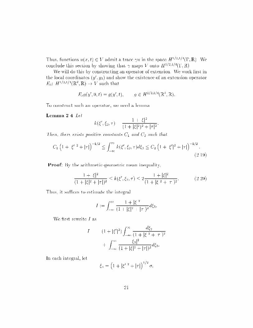
Lemma ��� Let
k���� ��� � � �� � j�j�
�� � j�j��� � j� j� �
Then� there exists positive constants C� and C� such that
C�
�� � j��j� � j� j
����� � Z �
��k���� ��� � �d�� � C�
�� � j��j� � j� j
������
������
Proof� By the arithmetic geometric mean inequality�
� � j�j��� � j�j� � j� j�� � k���� ��� � � � �
� � j�j��� � j�j� � j� j�� � ������
Thus� it su�ces to estimate the integral
I ��Z �
��� � j�j�
�� � j�j� � j� j��d���
We �rst rewrite I as
I � �� � j��j��Z �
��d��
�� � j�j� � j� j��
�Z �
��j��j�
�� � j�j� � j� j��d���
In each integral� let
�� ��� � j��j� � j� j
������
��

This leads to
I �� � j��j�
�� � j��j� � j� j����Z �
��d�
�� � ����
��� � j��j� � j� j
����� Z �
����
�� � ����d�� ������
Setting
C� �Z �
��d�
�� � ����and C� �
Z �
����
�� � ����d��
������ shows that
C�
�� � j��j� � j� j
����� � I � �C� � C���� � j��j� � j� j
������
as desired�We now construct the operator E�� Let
k���� � � �Z �
��k���� ��� � �d���
By lemma ���� we have
C� � k���� � ��� � j��j� � j� j���� � C��
For any g � H��������R��R�� we let
Fy��y��t �E�g� ���� �� � � �
k���� ��� � � k���� � �
Fy��t �g� ���� � ��
By construction� we have
Z �
��Fy��y��t �E�g� ��
�� ��� � �d�� � Fy��t �g� ���� � ��
and thus E�g � g� To show that E�g � V � we note that
jFy��y��t �E�g� ���� ��� � �j�k���� ��� � �
�k���� ��� � � k����� � �
jFy��t �g� ���� � �j�d���
��

Thus� integrating both sides over �� and using the de�nition of k���� � �� weget
Z �
��jFy��y��t �E�g� ���� ��� � �j�
k���� ��� � �d�� �
Z �
��k���� ��� � � k����� � �
jFy� �t �g� ���� � �j�d��
�jFy��t �g� ���� � �j�
k���� � �
� �
C��� � j��j� � j� j����jFy��t �g� ��
�� � �j��
Integrating this equation over �� and � immediately leads to
kE�gk�V �Z �
��
ZR�
Z �
��j�u��� � �j�k���� ��� � �
d��d��d�
� Ckgk�H��������R��R�� ������
We now use the operator E� to prove our claim on general surfaces ��Let v � H����������R� be given and consider the function
um�x� t� � ��mh��m��
���m �E���
�m
�����m v
��i� �x� t� � R� �R�
To show that um � V � we compute its L��R� � R� inner product with any � D�R� �R�� We have
hum� i �Z �
��
ZR�um�x� t��x� t�dxdt ������
�Z �
��
ZY����m ��m�y��E���
�m��
���m v��J ��m� �y���m�y�� t�dydt�
where J��m��y� denotes the Jacobian of the transformation from Om to Y �Now� the mapping of D�R� �R� de�ned by
�x� t� � ����m ��m�y��J ��m� �y���m�y�� t��
clearly de�nes a function of �y� t� which belongs to D�Y �R�� We set !m��equal to this map and let "!m�� denote the mapping obtained by extending!m �� �y� t� by zero to all y � R�� We note a few facts� First� we have theestimate
k"!m �� kL��R�H��R��� � C���kkL��R�H��R���� ������
��

Secondly� by ������� we have
hum� i �Z �
��
ZR�E�
���m��
���m v�
�"!m �� �y� t�dydt� �����
Lastly� and most importantly� the mappings "!m commute with the timederivative� That is�
"!m
��
�t
�
�
�t"!m �� � � D�R� �R�� �����
for each m�From the preceding considerations� we have these expressions for the dis
tributional time derivative of um�x� t��
h�um�t
� i � �hum� ��ti
� �Z �
��
ZR�E���
�m��
���m v�� "!m ����t� �y� t�dydt
� �Z �
��
ZR�E���
�m��
���m v��
�
�t"!m �� �y� t�dydt
�Z �
��
ZR�
�
�tE���
�m��
���m v�� "!m �� �y� t�dydt�
Taking absolute values� we deduce that
jh�um�t
� ij � C���k ��tE���
�m��
���m v��kL��H���R���kkL��H��R����
which shows that�um�t
�x� t� � L��R�H���R����
Since we already know that um�x� t� belong to L��R�H��R���� we concludethat um � V � Finally� by the linearity of the trace operator� it follows that
u �MXm��
um� ������
belongs to V and satis�es u � v�
��

� Mapping Properties of the Heat Operator
To study the heat operator # � ���t � � on functions u�x� t� which arede�ned for all �x� t� � R� � R� we require some special spaces of functions�As we shall show below� these spaces coincide with certain locally anisotropicSobolev spaces and are natural generalizations of the types of spaces used by����� ����� ���� in their treatments of the Laplace operator over unboundedregions� In this section� we �rst address the de�nition of these spaces andthen establish the mapping properties of the heat operator on them�
For all u � S�R� �R�� setkuk�W��� �
Z �
��
ZR�j�j�j�u��� � �j�d�d�� �����
kuk�W����� �Z �
��
ZR��j�j� � j� j�j�u��� � �j�d�d�� �����
kuk�V �Z �
��
ZR�
�j�j� � j� j�j�j��
�j�u��� � �j�d�d�� �����
where �u denotes the Fourier transform of u in space and time� Since theweight functions in ��������� are each locally integrable overR��R� it followsthat each of these expression is �nite for all u � S�R� �R�� The estimates
kukW��� � kukW����� � �kukV � u � S�R� �R�� �����
are easily derived� We denote by W���� W������ and V the completions ofS�R� � R� in the respective norms given by ���� ����� Thus we have thedense continuous inclusions
S�R� �R� � V � W����� �W����
Our �rst task is to show that these spaces can be identi�ed with a spaceof locally integrable functions� We will show this using the fact that thenorms given by ��������� di�er from the norms over the anisotropic Sobolevspaces H���� H������ and V �
kuk�H��� �Z �
��
ZR��� � j�j��j�u��� � �j�d�d�� ����
kuk�H����� �Z �
��
ZR��� � j�j� � j� j�j�u��� � �j�d�d�� ����
kuk�V �Z �
��
ZR�
�� � j�j� � j� j��� � j�j����
�j�u��� � �j�d�d�� �����
�

solely because their weight functions do not contain the constant term ��Let !��� denote any non negative function in D�R�� which satis�es � �
!��� � � for all � � R� with
!��� �
� j�j � ��� j�j � ��
For convenience� setB� � f� � R�� j�j � �g�
Given any u � S�R� �R�� let �u��� � � denote its Fourier transform� We set
�u���� � � � �� �!�����u��� � �� �����
�u���� � � � !����u��� � �� �����
and then de�ne u��x� t� and u��x� t� to be the respective inverse Fouriertransforms of �u���� � � and �u���� � �� Note that both u� and u� belong toS�R� �R� since u � S�R� �R�� Moreover�
u�x� t� � u��x� t� � u��x� t�� �x� t� � R� �R�In the next lemma� we establish useful estimates satis�ed by the functions
u��x� t� and u��x� t�� In stating this lemma� we denote by W ����R�� theBanach space
W ����R�� � f�x� � L�� jr�x�j � L��R��g�with associated norm
kkW ����R�� � supx�R�
�j�x�j� jr�x�j� �
Lemma ��� For any u � S�R� � R�� let u��x� t� and u��x� t� be de�ned asabove� Then�
ku�kH��� � �kukW��� �ku�kH����� � �kukW����� �ku�kV � �kukV �
������
andku�kL��R�W ����R��� � CkukW��� �
ku�kH����R�L��R��� � CkukW����� �
ku�kH��R�L��R��� � CkukV�������
�

Proof� Since �u���� � � is zero in a neighborhood of j�j � �� it is a simplematter to show ������� To show ������� we use the fact that the inverseFourier transform F��
x maps L��R�� boundedly into L��R��� Thus� to showthe �rst estimate of ������� it su�ces to show
Z �
��k�� � j�j��u���� � �k�L��R��d� � Ckuk�W��� � ������
Since !��� has compact support in B� and is bounded in absolute value byunity� we have
k�� � j�j��u���� � �kL��R�� � k �� � j�j���j�j�u���� � � kL��B��
� k �� � j�j���j�j�u��� � � kL��B��� ������
Applying the Cauchy Schwartz inequality to the right of ������� we get
k�� � j�j��u���� � �kL��R�� � k � � j�j�� kL��B��k j�j�u��� � � kL��R���
Since j�j�� is locally integrable in R�� it follows that
k�� � j�j��u���� � �kL��R�� � Ck j�j�u��� � � kL��R���
Squaring both sides of this inequality and integrating over � � we obtain �������To show the second estimate in ������� it su�ces to combine ������ with
the inequality Z �
��j� j k�u���� � �k�L��R��d� � Ckuk�W����� �
which follows from the trivial bound
k�u���� � �kL��R�� � Ck�u��� � �kL��R�� for all � � R�
Since
Fx�t
��u��t
��� � � � i� �u���� � �� ��� � � � R� �R�
the �nal estimate of ������ is veri�ed by combining ������ with
Z �
��j� j� k�u���� � �k�L��R��d� � C
Z �
��j� j� k j�j���u���� � � k�L��R��d�
� Ckuk�V�
��

Based on lemma ���� we can now show that each of the completed spacesW���� W������ and V may be identi�ed with a space of locally integrablefunctions� Speci�cally� in the case of W���� consider the Banach space
X � H��� � L��R�W ����R����
with associated norm
kuk�X � infu�u��u�
�ku�k�H��� � ku�k�L��R�W ����R���
��
The estimates given in lemma ��� immediately show that any sequence fukgof functions uk � S�R� � R� which is a Cauchy sequence in the W��� normis also a Cauchy sequence in X� Since X is complete� there exists a uniqueu � X which is the limit of the sequence fukg� It is readily checked thatequivalent Cauchy sequences� i�e�� two sequences fukg and fu�kg such that
limk��
kuk � u�kkW��� � ��
de�ne the same u � X� Thus� we can identify W��� with a subspace ofX� By similar considerations applied to W����� and V� we can make theseidenti�cations�
W��� � H��� � L��R�W ����R����
W����� � H����� � L��R�W ����R��� H����R� L��R����
V � V � L��R�W ����R��� H��R� L��R����
We remark that these inclusions are strict� They� however� clearly implythe next theorem which shows that the spacesW����W������ and V di�er fromthe anisotropic Sobolev spaces H���� H������ and V solely in their permittedbehavior as x tends to in�nity�
Theorem ��� For any � S�R��� there exists a constant C�� such that
kukH��� � C��kukW��� � ������
kukH����� � C��kukW����� � �����
kukV � C��kukV� �����
for all u � S�R� �R��
��

The importance of Theorem ��� is that we can immediately extend thetrace operator to the spaces W����� and V� Furthermore� we can concludethe following crucial theorem�
Theorem ��� Let � W����� � H����������R� denote the trace operator�Then� � � R� maps V onto H����������R��
Now� the time restriction operator R�� H����������R� � H����������R��is onto� Combining this fact with the above theorem gives the followingcorollary�
Corollary ��� The trace operator � � R� maps V onto H����������R���
Denote by W����� W�������� and V� the respective dual spaces of W����W������ and V� These are each spaces of tempered distributions which satisfythe inclusions
W���� � W������� � V� � S ��R� �R��Norms over these spaces may be de�ned using Fourier transforms as
kfk�W���� �Z �
��
ZR�
j �f��� � �j�j�j� d�d��
kfk�W������� �Z �
��
ZR�
j �f��� � �j�j�j� � j� jd�d��
kfk�V� �Z �
��
ZR�
j�j�j�j� � j� j� j
�f��� � �j�d�d��
The mapping properties of the heat operator # on W����� and W��� is thesubject of the next theorem�
Theorem ��� The heat operator # extends from S�R� � R� to an isomor�phism of W����� onto W������� and of W��� onto V�� Moreover�
Re h#u� ui � kuk�W��� for all u � W������ ������
Proof� The theorem is an easy consequence of the equality
Fx�t �#u� � �i� � j�j���u��� � �� u � S�R� �R��and the density of S�R� �R� in these spaces�
��

We now give an an alternative proof of the isomorphism of #� W����� �W�������� We do so because this method of proof extends to Dirichlet prob lems� which we address in section �� For all u� v � S�R� �R�� let
B�u� v� �Z �
��
ZR�
�u
�t�x� t�v�x� t� �ru�x� t�rv�x� t�dxdt� ������
where the bar denotes complex conjugation� By Parseval�s theorem�
B�u� v� �Z �
��
ZR�i� �u��� � ��v��� � � � j�j��u��� � ��v��� � �d�d� ������
A simple application of Cauchy Schwartz�s inequality shows that B satis�es
jB�u� v�j � kukW�����kvkW�����
for all u� v � S�R� � R�� Therefore� B uniquely extends to a boundedsesquilinear form on W����� �W������ In the next lemma� we show that thisextension satis�es conditions which readily imply that # is an isomorphism�
Lemma ��� There exists a bounded� linear operator H� W����� � W�����
such that
Re B�u� u�Hu� � kuk�W����� for all u � W������ ������
and
Re B�v �Hv� v� � kvk�W����� for all v � W������ ������
Proof� For each u � W������ let Hu�x� t� denote the function de�ned by
Fx�t�Hu���� � � � �isign�� ��u��� � �� ��� � � � R� �R� ������
This de�nes a mapping H which is an isometry on W������ This map isessentially the Hilbert transform in time� Readily� we see that
B�u� u� �Z �
��
ZR�i� j�u��� � �j� � j�j�j�u��� � �j�d�d�� ������
and
B�u�Hu� �Z �
��
ZR��j� j j�u��� � �j� � isign�� �j�j�j�u��� � �j�d�d�� ������
��

By subtracting ������ from ������ and then taking real parts� we get
Re B�u� u�Hu� � kuk�W����� �
Equation ������ is veri�ed analogously�
This lemma implies ��� Theorem ����� that #� W����� �W������� de�nedby
h#u� vi � B�u� v� for all v � W������ �����
is an isomorphism�
��

� Mapping Properties of the Single Layer
Heat Potential
In this section� we set out the mapping properties of the single layer heatpotential� We recall our notation for this operator
K�q�x� t� �Z t
�
Z�K�x� x�� t� t��q�x�� t��dx�dt�� �x� t� � ��R�� �����
Let C�� ���R�� denote the space of functions obtained by restricting func
tions "q�x� t� � D�� � R� to t � �� In Theorems ��� and ��� below� we willshow that K� extends from an operator on C�
� �� � R�� to an isomorphismfrom H������������R�� onto H����������R��� First� we need a preliminarylemma�
Lemma ��� For all q � C�� ���R��� let �q denote the tempered distribution
de�ned by
h�q� i �Z �
�
Z�q�x�� t���x�� t��dx�dt� for all � S�R� �R��
Then� with K denoting the fundamental solution to the heat equation and� convolution in the sense of distributions� we have K � �q � S ��R� � R��Furthermore�
Fx�t �K � �q� ��� � � �Fx�t ��q� ��� � �
�� � i�� �����
in the sense of tempered distributions�
Proof� Since q equals zero for large t� �q is a distribution with compactsupport� Because K � S ��R� � R�� standard results of distribution theory�cf�� ���� pp� ��� ������ show that K ��q � S ��R��R� and that ����� holds�
We now establish a basic factorization result which equates the operatorK� on C�
� ���R�� with an operator whose extension to H������������R�� isimmediate�
Theorem ��� Let #� W����� � W������� denote the heat operator and ��W����� � H����������R�� the trace operator� The integral operator K� de�nedon C�
� �� � R�� by ����� agrees with the composition � � #�� � �� andconsequently extends to a bounded linear operator of H������������R�� intoH����������R���
��

Proof� Since �� W����� � H����������R�� is bounded� its adjoint �� maps
H������������R�� boundedly into W�������� For each q � H������������R���de�ne uq � #����q� Since #� W����� � W������� is an isomorphism� wehave
kuqkW����� � CkqkH������������R��� �����
By Theorem ��� the Fourier transform of uq is
Fx�t �uq� ��� � � �Fx�t
���q
���� � �
j�j� � i�� ��� � � � R� �R� �����
Now� suppose that q � C�� �� �R��� Since ��q is de�ned by
h��q� vi � hq� �vi for all v � W������ ����
it follows that ��q agrees with �q �de�ned in Lemma ����� Therefore� byLemma ���� we have
uq�x� t� � K � �q
�Z t
�
Z�K�x� x�� t� t��q�x�� t��dx�dt�� �x� t� � R� �R�
Taking the trace of uq� we get
� �#�� ���q �Z t
�
Z�K�x�x�� t� t��q�x�� t��dx�dt�� �x� t� � ��R�� ����
Thus� ���� shows that on C�� ���R�� the single layer heat potential K�
coincides with the bounded operator �#����� Because C�� ���R�� is dense
in H����������� �R��� the operator K� uniquely extends to H����������� �R���
We now give one of the main results of this paper�
Theorem ��� The single layer heat potential K� � � � #�� � �� is anisomorphism of H������������R�� onto H����������R��� Furthermore� it sat�is�es the coercivity estimate
Re hq�K�qi � ckqk�H������������R��� �����
for some positive constant c�
��

Proof� We consider the duality pairing hq�K�qi for q � H������������R���Using the de�nition of ��� we have
hq�K�qi � h��q�#����qi�
Now� since �� V � H����������R�� is surjective� it follows � see ����Theorems ���� and ������ that its adjoint �� maps H������������R�� iso morphically onto a closed subspace of V�� Hence� there exists some positiveconstant c such that
k��qkV� � ckqkH������������R�� for all q � H������������R��� �����
The argument
Re hq�K�qi � Re h##����q�#����qi� k#����qk�W��� by �������
� ck��qk�V� by Theorem ���
� ckqk�H������������R��
� by ������
then proves the coercivity statement� By the Lax Milgram theorem� K� isan isomorphism�
In studying the regularity of the single layer operator K�� it will be con venient to work mainly with the operator "K� � #���� We have
K� � R�"K�R
���
where R�� H����������R�� H����������R�� denotes the time restriction op erator� Clearly� "K� de�nes an isomorphismofH������������R� ontoH����������R��
For later use� we note that this implies that the adjoint operator "K�� ��#����� is also an isomorphism of H������������R� onto H����������R��
The map "K�� extends the backward heat potential
"K��p�x� t� �Z �
t
Z�K�x� x�� t� � t�p�x�� t��dx�dt�� �x� t� � R� �R�
��

We now adapt an argument due to Nedelec and Planchard which further
characterizes the inverse operator "K��� � The starting point is a variationalformulation of the homogeneous Dirichlet problem
�u
�t��u � f on R
�n��R �����
u � � on ��R� ������
To treat this problem� let
W������ � fu � W������ u � �g�
Thus� W������ corresponds to the subspace of W����� functions u�x� t� which
vanish for x � �� Equivalently� W������ is the closure in the W����� norm of
S�R�n� �R�� �Note therefore that the dual space �W������ �� is contained in
D�R�n� � R� but not in D�R� �R��� Since W������ is a subspace of W������
the bilinear form B introduced in ������
B�u� v� �Z �
��
ZR��i� � j�j���u��� � ��v��� � �d�d��
is well de�ned for all u� v � W������ � Thus� for any f � �W�����
� ��� we may
consider the variational problem of �nding u � W������ such that
B�u� v� � hf� vi for all v � W������ ������
A standard argument shows how Problem ������ extends the Dirichletproblem ����������� Let u denote any smooth solution u to problem �������By a smooth solution to ������� we mean a C�R� �R� function u �vanishingsu�ciently rapidly at in�nity say� which is twice continuously di�erentiablein each of the sets ��R and �c �R� Clearly� for such a function� we have
B�u� v� �Z �
��
Z
��u
�t�x� t���u�x� t�
v�x� t� dx dt
�Z �
��
Zc
��u
�t�x� t���u�x� t�
v�x� t� dx dt�
�

for any v in the Schwartz class S�R� �R�� Hence� by Green�s theorem�
B�u� v� �Z �
��
ZR�
��u
�t�x� t���u�x� t�
v�x� t� dx dt
�Z �
��
Z�
��u
�n�x� t� jint �
�u
�n�x� t� jext
v�x� t�dxdt�
v � S�R� �R��Since u by assumption solves ������� it follows that
Z �
��
ZR�
��u
�t�x� t���u�x� t�
v�x� t� dx dt �
Z �
��
ZR�f�x� t�v�x� t� dx dt�
for any arbitrary function v � S�R��R� which vanishes on the boundary ��Hence� u satis�es ������
Lemma ��� The variational problem ������ de�nes an isomorphism of u �W�����
� onto f ��W�����
�
��and consequently extends the homogeneous Dirich�
let problem ���������
Proof� As in the proof of Lemma ��� let H denote the Hilbert transformde�ned by
Fx�t�Hu���� � � � �isign�� �Fx�t�u���� � � for all u � S ��R� �R��Already� we have shown that
B �u� �I �H�u� � kuk�W����� for all u � W������
and
B ��I �H�v� v� � kvk�W����� for all v � W������
������
Since the Hilbert transform is an operator only in time� it is easy to seethat H maps W�����
� onto W������ � This along with ������ clearly implies the
lemma�Using trace theory� we extend this result to a Dirichlet problem with in
homogeneous boundary data in the next theorem� Without loss of generality�we assume that the forcing function f equals zero� �We can always add tosolutions given below a function uf determined by lemma ��� which vanisheson the boundary and satis�es �������
�

Theorem ��� For each g � H����������R�� there exists a unique solutionu � W����� to the Dirichlet problem
�u
�t��u � � on R
�n��R� ������
u � g on ��R� ������
Proof� Given g � H����������R�� we may �nd ug � W����� such that ug �
g� If we let u� � W������ denote the unique solution to
B�u�� v� � �B�ug� v� for all v � W������ �
we then obtain a solution u � ug � u� � W����� with u � g� Noting that usatis�es
B�u� v� � � for all v � W������ � �����
it easily follows that this solution is unique� that is� independent of theextension of g to W������
We continue to denote by u the solution to the Dirichlet problem ������������ We will de�ne an interior and exterior normal derivative of u in thefunction space H������������R�� First� we de�ne the spaces W�������c � R�andW��������R�� Let R��c� denote the restriction operator R��c�� S�R��R� � C���c � R�� By density� R��c� extends to W������ We now de�neW�������c�R� to be the image of R��c� on W������ We analogously de�neW��������R�� Poincar$e�s lemma shows that this latter space coincides withH��������R�� We set
B�u� v% �c� �Z �
��
Zci�F t�u��x� � �Ft�v��x� � �
�rF t�u��x� � �rFt�v��x� � �dxd��
for all u� v � W�������c�R��
and de�ne B�u� v% �� analogously�Now� let u represent the solution to ����������� and denote by u� and
u� its restrictions to � and �c� We de�ne linear functionals �u���n and�u���n over H����������R� as
h�u��n
� gi � B�u� Eg% �� for all g � H����������R�� �����
��

h�u��n
� gi � B�u� Eg% �c� for all g � H����������R�� ������
where Eg denotes any bounded extension of g � H����������R� to W������Because u solves ����������� and thus ������ it is easy to check that �����and ������ uniquely de�ne �u���n and �u���n in H������������R�� �Thatis� they are independent of the choice of extension E�� By applying Green�stheorem� it can be shown that ����� and ������ agree with the classicalde�nitions of these normal derivatives when u is a smooth solution�
Consider
q ���u��n
� �u��n
� ������
Clearly� q belongs to H������������R� and solves
hq� gi � B�u� Eg� for all g � H����������R�� ������
Since ������ holds independent of the choice of extension�
hq� vi � B�u� v� for all v � W������ ������
Equivalently� �q � #u� so #���q � u � g� or
"K�q � g� ������
��

� Regularity of the Single Layer Operator
The objective of this section is to establish a regularity theory for the singlelayer operator K�� Most of our e�orts in this section will concentrate onstudying the regularity of the related operator "K� and proving Theorem ���Once we prove this theorem� we shall apply the mappings properties of therestriction and extension operator to conclude regularity results for the op erator K��
Theorem ��� For all r � �� the operator "K� maps Hr�����r���������R� ontoHr�����r���������R��
Thanks to interpolation theory ��� p� ��� we may con�ne our attentionto non negative integer values of r� We will denote such values by m�The proof of Theorem �� naturally divides into two separate investiga tions� In section ��� we will show that the map "K�� Hr�����r���������R� �Hr�����r���������R� is bounded� In section ��� we will then show that thismapping is also surjective and hence an isomorphism�
��� Boundedness
For any non negative integer m� let q � Hm�����m���������R� be given� Ourgoal in this subsection is to show the estimate
k "K�qkHm�����m���������R� � C�m�kqkHm�����m���������R��
for some positive constant C which depends on m� We will prove this byestablishing the pair of estimates
k "K�qkHm�������R�L����� � C��m�kqkHm�����m���������R�� ����
and
k "K�qkL��R�Hm�������� � C��m�kqkHm�����m���������R�� ����
Our �rst lemma addresses estimate ���� and considers the regularity ofthe operator "K� with respect to time� For convenience� we set
Qs � Hs�����R� L����� Hs�R�H�������� s � R�and note that
�Q�s�� � Hs�����R� L����� �Hs�R�H��������� s � R�
��

Theorem ��� The single layer operator "K� maps �Q�s�� into Qs for alls � ��
Observe that Theorem �� reduces to Theorem ��� for s � � becauseQ� � H����������R� and
�Q��� � H�����R� L����� � L��R�H��������
� H������������R��
This theorem implies ���� since
kqkHs�����R�L����� � kqkQs� s � R�and
kqk�Q�s�� � kqkHs�����R�L������ s � R�� kqkHs�����s�������R�� s � ����
Its proof requires a de�nition� For each � � R� we de�ne the operator d�t �S ��R� �R�� S ��R� �R� by
F t�d�t u��x� � � � �� � j� j�����F t �u� �x� � �� �x� � � � R� �R�
The mapping d�t naturally extends the notion of a di�erentiation operatorin time to distributions and for all real orders� It de�nes an isomorphismbetween a variety of Sobolev spaces� For example� it maps Hs�R�Hr�R���isometrically onto Hs���R�Hr�R��� for all real numbers r� s� and �� It isalso easy to see that d�t � W����� �W����� and d�t � W������� �W������� arebounded for all � � ��
We also introduce the analogously de�ned operator S ����R�� S����R�which we also denote by d�t � Clearly� d�t maps Qs isomorphically onto Qs��for all s�� � R� Because
kd�t qk�Q��s � infq���q
���d
�t qkq��k�Hs�����R�L����� � kq��k�Hs�R�H���������
� infq��q��q
kd�t q�k�Hs�����R�L����� � kd�t q�k�Hs�R�H���������
� infq��q��q
kq�k�Hs�������R�L����� � kq�k�Hs���R�H���������
� kqk�Q�s�����it follows that d�t also maps �Q�s�� into �Q�s���� for all s� � � R�
��

Proof of Theorem ��� Let s � � be �xed� We must show that "K�q � Qs
for all q � �Q�s��� Equivalently� we will show that
dst "K�q � H����������R� for all q � �Q�s��� ����
To show ����� we establish these two claims�
"K�dstq � H����������R� for all q � �Q�s��� ����
anddst
"K�q � "K�dstq for all q � D�� �R�� ���
By a simple density argument� ���� then follows from ���� and ����Since dst � �Q�s�� � �Q��� and "K�� �Q��� � Q� are isomorphisms� ���� is
apparent� To prove ���� we note some identities� For example� by Fouriertransforms� it follows that
d�st #��f � #��d�st f for all f � S ��R� �R�� ���
Analogously� if we let S� equal the subspaces �of S ��R� �R��S� � f � W������ d�st � W�����g�
we can extend� � d�st
� �
�d�st �
� for all � S�R� �R�� ����
to � S�� Observe that S� � W����� while S� is identical to W������ Notealso that ���� implies
d�st �p � �d�st p for all p � H������������R�� ����
since for p � H������������R� and � W������ we have
hd�st �p� i � hp� d�st i� hp� d�st i� by �����
� h�d�st p� i�Now� for q � D�� �R�� we have
#�� �dstq � dst d�st #�� �dstq
� dst #�� d�st �dstq� by ��� and �����
� dst #�� � d�st dstq� by �����
� dst"K�q�
which proves ��� and completes the proof of the theorem�
��

We turn to proving estimate ����� Here� the use of localization is neces sary� We shall follow the notation of section ���� though this time we do notindex the sets� Hence� let � denote a C� di�eomorphism de�ned over someopen set O � R� which maps
O onto Y � f�y�� y��� jy�j � �� �� � y� � �g�and
O � onto Y� � fy � Y � y� � �g�
We again denote the inverse mapping of � by � and let � � D�O� denotethe cuto� function which corresponds to the set O� Finally� we recall theoperators
�� �w� �x� t� � w���x�� t� w � H������Y�R��
�� �u� �y� t� � u���y�� t�� u � H������O�R��
Now� for q � H������������R�� let uq � #���q� We need to consider thetrace of uq since this is by de�nition the image "K�q� Using the principles oflocalization� we can instead work in local coordinates and consider the traceof wq � ����uq�� Clearly�
kwqkH������Y�R� � CkqkH������������R�� ����
In the next theorem� which is the key to proving ����� we consider the exis tence of the higher order spatial derivatives of wq� We will use the multiindexnotation
�� ����
�y�
���
�y�
���
�y��
where � � ���� ��� ��� � N��
Theorem ��� Let m be a non�negative integer and � any multiindex withj�j � m and �� � �� Then� there exists a positive constant C which dependson m such that
k��wqkH������Y�R� � CkqkHm�����m���������R�� �����
��

This is a standard result in the regularity theory of boundary value prob lems� The condition �� � � occurs since it is necessary to insure the distri butional equality
���f � ���f� f � D��R� �R��Although its rigorous proof �based on the method of �nite di�erences� isstraightforward� it is rather tedious� Thus� we shall give the proof in Ap pendix A�
Although Theorem �� does not say that wq belongs to L��R�Hm���Y ���it does supply enough information to conclude that the trace of wq� �i�e��wq�� belongs to L��R�Hm��������� This is an obvious corollary to the nextlemma�
Lemma ��� For any non�negative integer m� let �x� � H��R�� satisfy
�� � H��R���
for all multiindices � with j�j � m and �� � �� Then� � Hm�����R�� andsatis�es
kk�Hm�����R�� � C�m�Xj�j�m
����
k��k�L��R�H��R���� �����
Proof� By Fourier transforms� The basic equation relating to its trace is
Fy� �� ���� �
Z �
������� ���d��� �����
where � denotes the Fourier transform of � Setting
k���� ��� ��� � j��j�
�m�� �� � j�j�
�����
we apply the Cauchy Schwartz inequality to ����� to get
jFy�������j� � I����
Z �
��k����� ���j����� ���j�d���
where
I���� ��� � j��j�
��m Z �
��d��
� � j�j�� C
�� � j��j�
���m������
��
Therefore�
�� � j��j�
�m���� jFy�������j� � C
Z �
��k����� ���j����� ���j�d��� �����
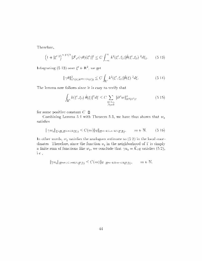
Integrating ����� over �� � R�� we get
kk�L��R�Hm�������� � CZR�k����� ���j����j�d�� �����
The lemma now follows since it is easy to verify that
ZR�k���� ���j����j�d� � C
Xj�j�m
����
k��wk�H��R��� ����
for some positive constant C�Combining Lemma �� with Theorem ��� we have thus shown that wq
satis�es
kwqkL��R�Hm�����Y�� � C�m�kqkHm�����m�������R�� m � N� ����
In other words� wq satis�es the analogous estimate to ���� in the local coor dinates� Therefore� since the function uq in the neighborhood of � is simplya �nite sum of functions like wq� we conclude that uq � "K�q satis�es �����i�e��
kuqkHm�����m�������R� � C�m�kqkHm�����m�������R�� m � N�
��

��� Surjectivity
To complete the proof of Theorem ��� it remains to show the surjectivity ofthe map "K�� Hr�����r���������R�� Hr�����r���������R�� As we shall see� thissurjectivity follows from regularity results for the Dirichlet problem �������������� Over the interior set � � R� the regularity theorem we need is wellknown ��� Theorem ��� and Theorem ��� and is recalled for convenience�
Theorem ��� Let � denote any bounded� open set in R�� Then� for eachnon�negative real number r� the Dirichlet problem
�u
�t��u � F on ��R�
u � g on ��R�
de�nes an isomorphism of u � Hr���r���������R� onto
�F� g� � Hr���r���������R��Hr�����r���������R��
To extend this result to the Dirichlet problem posed over the exterior set�we need to introduce a new class of function spaces� We shall �rst de�nethese spaces over R� � R and then by restriction over �c � R� For eachpositive integer m and u � S�R� �R�� set
kuk�Wm�m�� �Z �
��
ZR��� � j�j� � j� j�m���j�j� � j� j�j�u��� � �j�d�d��
where �u again denotes the Fourier transform of u� We now de�ne the spacesWm�m�� as the completions of S�R� �R� in these norms�
Clearly� this de�nition agrees with the de�nition of W����� when m � �and
Wk�k�� �Wm�m�� for integers � � m � k�
By an identical argument to the one used in section �� we can show that�x�u�x� t� � Hm�m�� if �x� � S�R�� and u�x� t� � Wm�m��� The spacesWk�k����c�R� are de�ned as the space of restrictions to �c � R of Wm�m���The next lemma shows our motivation for introducing these spaces�
Lemma ��� The heat operator # maps Wm�m�� onto Hm���m����W�������
for all integers m � ��
�

Proof� Observe that the lemma reduces to Theorem �� for m � � since
W������� � H��������
Thus� we assume that m � �� There is no natural embedding betweenW������� and Hm���m���� for such m�
Let u � S�R� � R� and let �u denote its Fourier transform in space andtime� Clearly�
Fx�t �#u� ��� � � � �i� � j�j���u��� � �� ��� � � � R� �R�implies
�
��j�j� � j� j�j�u��� � �j� � jFx�t �#u� ��� � �j�
j�j� � j� j � �j�j� � j� j�j�u��� � �j�� �����
We now multiply this equation by ��� j�j� � j� j�m�� and then integrate over��� � �� Using the de�nition of Wm�m��� we get
�
�kuk�Wm�m�� �
Z �
��
ZR�km��� � �jFx�t �#u� ��� � �j�d�d� � kuk�Wm�m��
where
km��� � � ��� � j�j� � j� j�m��
j�j� � j� j �
To complete the proof� it su�ces to show that
f � Z �
��
ZR�km��� � �jFx�t �f� ��� � �j�d�d�
����� �����
de�nes a norm over Hm���m���� W������� which is equivalent to
f �nkfk�Hm���m���� � kfk�W�������
o����
But� since m � � and
kfk�W������� �Z �
��
ZR�� j�j� � j� j ���j �f��� � �j�d�d��
and
kfk�Hm���m���� �Z �
��
ZR�� � � j�j� � j� j �m��j �f ��� � �j�d�d��
�

this is an obvious corollary of the binomial theorem�
Remark� Intuitively� the reason that theW������� term must be explicitly in cluded above is because the spaceWm�m�� imprecisely describes the behaviorof solutions at in�nity�
Using Lemma �� Theorem � and the principles of localization� thenext result can be shown� As before� the proof is tedious but straightforward�Thus� we give the proof in appendix B�
Theorem �� Let g � Hm�����m���������R� for some integer m � �� Then�the solution u � W����� to
�u
�t��u � � on R
�n��R� �����
u � g on ��R� �����
satis�es
uj � Hm���m���������R� and ujc � Wm���m��������c�R��
From Theorem ��� the surjectivity of the mapping "K� is easily deduced�
Theorem ��� For all r � �� the operator "K� maps Hr�����r���������R� ontoHr�����r���������R��
Proof� Suppose that r equals a non negative integerm� Given g � Hm�����m���������R��let u denote the solution to ���� ����� Set
q ��u��n
� �u��n
�
From Theorem �� and a trace theorem �cf�� the remark after Theo rem ����� it follows that each of the normal derivatives satis�es the inclusions
�u��n
� Hm�����m���������R�
and�u��n
� Hm�����m���������R��
Hence� we have q � Hm�����m���������R� and by ������ and ������� "K�q � g�The surjectivity for all non negative values of r follows by interpolation�
��

With the proof of Theorem �� complete� we apply it to consider theregularity of the operator K� in the next theorem�
Theorem ��� The single layer potential K� maps
Hr�����r�������� ���R�� onto H
r�����r�������� ���R��� for all r � ��
To prove this result� we need a few preliminary results
Theorem ��� The heat operator # maps fu � W����� � u � � t � �gisomorphically onto fF � W������� � F � �� t � �g�
A proof of this result is given in ���� pages ��������� We state a usefulcorollary to this result�
Corollary ���� Let g � H����������R� be such that g � � almost every�where for t � �� Then� the unique solution u � W����� to the Dirichletproblem ���������� equals zero for t � ��
Proof� Let g � H����������R� with g � � for t � � be given� The cruxof the matter is to note there exists a trace extension Eg � W����� of gwhich satis�es Eg � � for t � �� It is not to hard to see that there aremany extensions which satisfy this� For example� in the local coordinates�the multiplication map
g�y��� ��yn�g�y��� �y�� y�� � R��
where � � D�R� with ���� � � is clearly such an extension� as is the extensionde�ned by it using the procedure described in section ����
Now� recall how the Dirichlet solution u is determined� We have thatu � Eg � u� where u� � W�����
� is determined by
h#u�� vi � �h#Eg� vi for all v � W������ �
Since Eg vanishes for t � �� it follows that #Eg also vanishes for t � � andby Theorem ���� so does u��
In the next theorem� we show that "K� satis�es properties quite analogousto the ones in Theorem ��� satis�ed by the heat operator #�
Theorem ���� The operator "K� maps fq � H������������R� � q � �� t � �gisomorphically onto fg � H����������R� � g � �� t � ��g
��

Proof� Let q � H������������R� with support in t � � be given� Since thetrace operator is purely a spatial operator� it is easy to see that �q �W������� also has support in t � �� Hence� by Theorem ���� the function#���q � W����� has support in t � �� Thus� so does #���q � "K�q�
Conversely� let g � H����������R� with support in t � � be given� Itsu�ces to show that
h "K��� g� �i � ��
for any arbitrarily �xed � � H���������R� which equals zero for t � �� Toshow this� let ug denote the unique solution to the Dirichlet problem ������������ By Corollary ���� ug vanishes for t � �� Now� recall our discussion at
the end of section �� In this section� we showed that "K��� g agrees with thejump in the normal derivatives of ug across the boundary �� Clearly� thesenormal derivatives and thus q vanish for t ���
It is now a simple matter to prove Theorem ��� Given any q in theSobolev space H
r�����r�������� ���R��� it follows that its zero extension R��q
satis�esR��q � Hr�����r���������R��
and vanishes for t � �� Hence� "K�R��q belongs to Hr�����r���������R� and
vanishes for t � �� By de�nition� its restriction to R�� namely R�"K�R
��q �
K�q belongs to Hr�����r�������� ���R��� The other direction follows with equal
ease�
��

� Galerkin Discretization of the First Kind
Boundary Integral Equation
In the remaining sections� we discuss the numerical solution of the �rst kindboundary integral equation
K�q�x� t� ��Z t
�
Z�K�x� y� t� s�q�y� s�dyds � F �x� t�� �x� t� � � �R�
����by Galerkin methods� The coercivity of single layer potential K� impliesthe quasioptimality of Galerkin approximations� That is� if Qh denotes anyclosed subspace of H������������R�� and qh � Qh the unique solution to theGalerkin equations
hp�K�qhi � hp� F i for all p � Qh� ����
thenkq � qhkH������������R�� � C inf
q�h�Qh
kq � q�hkH������������R��� ����
In section ��� we describe a standard class of tensor product spacesQdx�dth � V dt
h � Xdxh which are based on polynomials of degree dt in time
and polynomials of degree dx in space� In sections �� and ��� we considerthe implementation of the Galerkin method using the space V �
h of piecewiseconstants in time� In section ��� we consider the Galerkin equations whenhigher order polynomials are used in time�
��� Construction of the Trial Space
Let ht denote the stepsize of a uniform partition of R�� We de�ne V �h as the
space of piecewise constant functions subordinate to this mesh� This spaceis conveniently described as the span of the basis functions
�k�t� �
�� �k � ��ht � t � kht��� otherwise
� k � �� �� � � � �
The L� projection operator Pt� L��R��� V �h is de�ned by
Ptu�t� ��Xk��
�
hthu� �ki�k�t�� ����
�

Note that Pt extends to an operator on Hs��R�� for s� � ����� since thefunctions �k belong to Hs��R�� for s � ���� Analogously� for any dt � �� wede�ne V dt
h to be the space of piecewise� discontinuous polynomials of degreedt�
A description of Xh is more involved� We assume that � can be dividedinto M closed subsets �m such that
� �M�m��
�m� and �m� �m� is a curve� a point� or empty for m� �� m��
���We assume that each piece �m can be smoothly mapped in a � to � fashiononto the unit square
�S� � f���� ���� � � ��� �� � �g�We denote the mappings �m � �S� by &m and assume that each &m is therestriction to � of some C� di�eomorphism which maps an open R� neigh borhood of �m onto some open R� neighborhood of �S�� Thus� it makes senseto de�ne the inverse mappings !m� �S� � �m� Without loss of generality� wewill suppose that the various Jacobians of &m and !m are strictly positive�
The mappings !m will be used to de�ne interpolation over �� For thispurpose� it is necessary that they piece together correctly� Precisely� werequire that &m� �!m� � &m���m� �m�� � &m���m� �m�� is an isometryif �m� �m� �� ��Remark� Our assumptions on � are fairly general and apply to most surfacesencountered in practice� For example� they apply to any convex surface� Thesame sort of assumptions have been made by ���� ����� and ����� An importantcase which does not require an elaborate boundary decomposition is when �is a polygonal surface� Our analysis� however� does not strictly apply to thiscase since regularity assumptions which are justi�ed on smooth surfaces byour regularity results fail to hold on polygonal surfaces�
For each m� let �Rm
h denote a regular triangulation of �S� by rectangularelements� For each rectangle �r � �R� de�ne curvilinear rectangles r by
r � fx � R�� &m�x� � �rg�Let Rm
h be the set of all such rectangles r as �r varies in �Rm
h � The union
Rh ��m
Rmh �
�

is a triangulation of the surface � by curvilinear rectangles� We set
hx � maxr�Rh
diam r�
The spaces Xdxh are now de�ned as images of spaces of piecewise poly
nomials de�ned over the triangulation �Rh� For any non negative integer dxand any set �r � �Rh� let �P��r� dx� denote the tensor product space of dx degreepolynomials in each variable� We then de�ne
Xdxh � fqh � L����� qhjr �!m � �P��r� dx�% for all r � Rm
h � m � �� � � � �Mg�
Basis functions for Xdxh are de�ned as the images of standard polynomial
basis functions� Let ��j���� ��� �for j � � to �dx � ���� denote the basisfunctions of P� �S��� �For example� if dx � �� these four functions are
������� ��� � ������������ ��� � ���� � ����
������� ��� � ��� ������������� ��� � ��� ����� � ����
Given r � Rmh � let �r � !m�r� and denote by �' the dilation from �r onto
�S�� Then� for each r � Rmh � it is easy to check that the set of functions
�jr � ��j � �' � &m� j � �� � � � � �dx � ���� ���
de�nes a basis for Xhjr� Thus� the collection of functions
f�jr � j � �� � � � �dx � ���� r � Rhg
forms a basis for Xdxh In formulating the Galerkin equations� it will be conve
nient to reindex the basis functions in Xdxh and to denote them by f���x�g�
Note that the doubly indexed set f���x��n�t�g forms a basis of Qdt�dxh �
�

��� Implementation
The Galerkin equations ���� in the subspace Q���h are the linear system
h���n�K�qhi � h���n� F i� � � �� �� � � � � Nx� n �Z�� ����
whereNx denotes the dimension ofXh� Since the Galerkin solution qh belongsto Q���
h � we can expand it in terms of the Qh basis functions as
qh�x� t� ��Xk��
NxX���
q�k���x��k�t��
Substituting this expansion into ����� we get
�Xk��
NxX���
h���n�K����kiq�k � h���n� F i� � � �� � � � � Nx� n �Z�� ����
Since ���� is indexed by four integers� its solution requires some orderingor partitioning of the unknowns� For each positive integer n� we de�ne vectors�qn of length Nx by
�qn �
�BBBB�
q��nq��n���
qNx�n
�CCCCA � n �Z��
Similarly� we let �Fn denote vectors of length Nx whose components are givenby
��Fn�� �Z����x�
Z nht
�n���htF �x� t�dtdx� � � � � Nx� n �Z��
Finally� we de�ne square matrices� Gnk � of order Nx for each n� k �Z� by
�Gn�k���� �Z�
Z����x�gn�k�x� x�����x��dx�dx� ����
where for any x � R�� gn�k�x� denotes
gn�k�x� �Z nht
�n���ht
Z kht
�k���htK�x� t� t��dt�dt� �����
�

With this notation� the Galerkin system ���� partitions in the form
�BBBB�G�� G�� G�� � � �G�� G�� G�� � � �G�� G�� G�� � � ����
������
� � �
�CCCCA
�BBBB��q��q��q����
�CCCCA �
�BBBBB�
�F�
�F�
�F����
�CCCCCA � �����
Nowh�n�K��ki � � for n � k� �����
so Gnk � � for n � k� Thus� ����� has the block lower triangular form
�BBBB�G�� � � � � �G�� G�� � � � �G�� G�� G�� � � ����
������
� � �
�CCCCA
�BBBB��q��q��q����
�CCCCA �
�BBBBB�
�F�
�F�
�F����
�CCCCCA � �����
We point out that this lower triangular form occurs because the supports�k��t� and �k��t� for di�erent values of k� and k� are disjoint� Therefore� alower triangular form would still result if one de�ned Vh using a non uniformmesh�
Expanding ����� out� we get the set of order Nx linear systems
nXk��
Gnk�qk � �Fn� n � �� �� � � � � Nx�
or
Gnn�qn � �Fn �n��Xk��
Gnk�qk� n � �� �� � � � � Nt �����
Observe how ����� successively determines the solution at each timestep asthe solution to a linear system of order Nx� We remark that the invertibilityof the matrices Gnn is a direct consequence of the coercivity of the operatorK�� �Consider the pairing hp�K�pi for any p � Q���
h which is support in theinterval �n� ��ht � t � nht��
For constant time steps� an important savings occurs since the matricesGn�k satisfy
Gn�k� � Gn�k� when n� � k� � n� � k�� ����
�
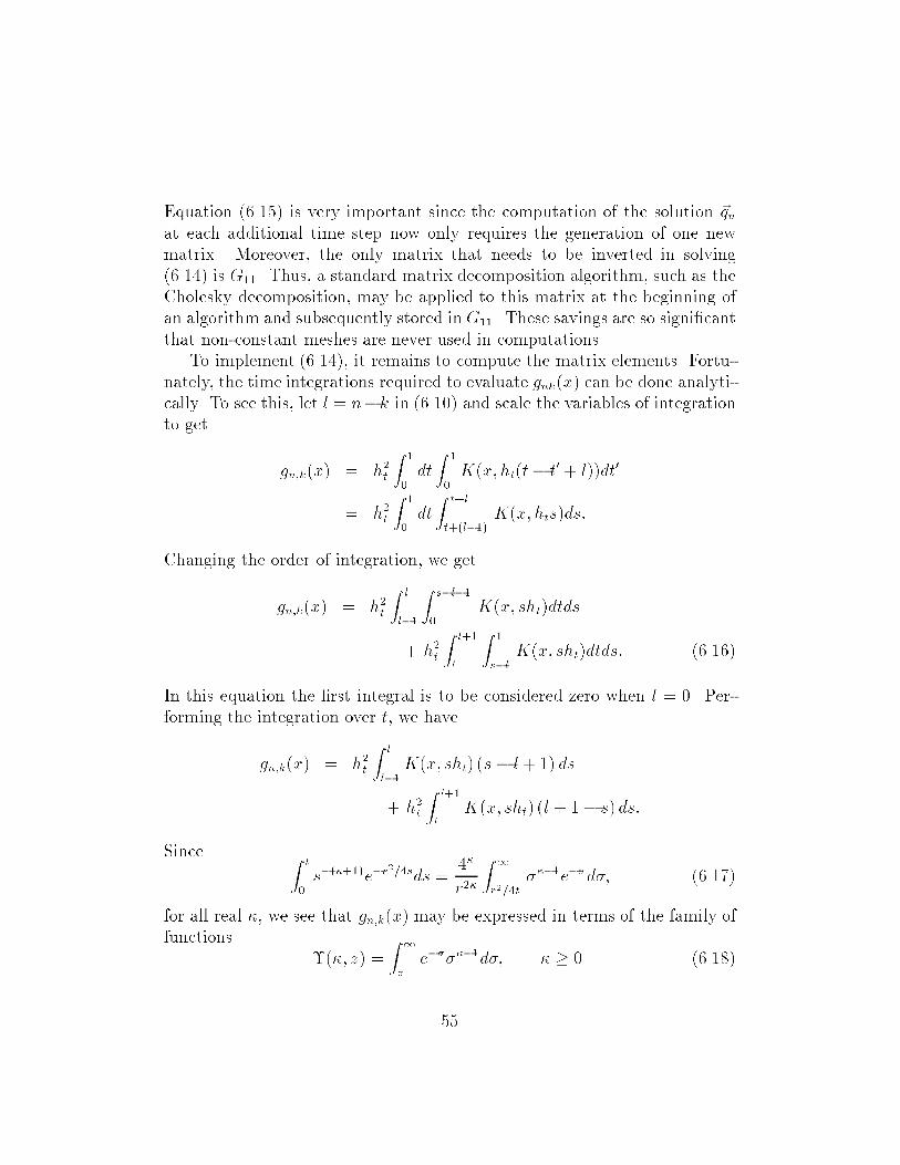
Equation ���� is very important since the computation of the solution �qnat each additional time step now only requires the generation of one newmatrix� Moreover� the only matrix that needs to be inverted in solving����� is G��� Thus� a standard matrix decomposition algorithm� such as theCholesky decomposition� may be applied to this matrix at the beginning ofan algorithm and subsequently stored in G��� These savings are so signi�cantthat non constant meshes are never used in computations�
To implement ������ it remains to compute the matrix elements� Fortu nately� the time integrations required to evaluate gnk�x� can be done analyti cally� To see this� let l � n�k in ����� and scale the variables of integrationto get
gn�k�x� � h�t
Z �
�dtZ �
�K�x� ht�t� t� � l��dt�
� h�t
Z �
�dtZ t�l
t��l���K�x� hts�ds�
Changing the order of integration� we get
gn�k�x� � h�t
Z l
l��
Z s�l��
�K�x� sht�dtds
� h�t
Z l��
l
Z �
s�lK�x� sht�dtds� ����
In this equation the �rst integral is to be considered zero when l � �� Per forming the integration over t� we have
gn�k�x� � h�t
Z l
l��K�x� sht� �s� l� �� ds
� h�t
Z l��
lK�x� sht� �l � �� s� ds�
Since Z t
�s�����e�r
���sds ��
r�
Z �
r���t���e��d�� �����
for all real �� we see that gn�k�x� may be expressed in terms of the family offunctions
(��� z� �Z �
ze�����d�� � � �� �����

Setting
al �x�
�lht� l �Z�� �����
and working out the details� we get
�����
htgn�k�x� �
�
r�l� � �
pa�� �(�a���� ���� �(�al� �����
� �
r�l� � �
pa�� �(�al� ���� �(�al��� �����
�h�le�al � �l � ��e�al�� � �l� ��e�al��
i� �����
for all values of �n� k� such that l � �� �When l � �� one uses the limits
limz��
ze���z � � and limz��(�z� � ���
The appropriate expression for gn�n�x� is
gn�n�x� �ht
�����
��� �
pa��
�
r(�a�� ���� � e�a�
��
The functions ( are known as the complementary incomplete gammafunctions and are customarily denoted by ���� z� �we avoid this notationbecause it con�icts with our notation for the spatial surface�� They have beenextensively studied and tabulated� For all positive values of �� they tend toa �nite limit as z tends to zero �namely� the value of the complete gammafunction�� When z tends to in�nity� these functions decrease exponentiallyto zero� More precisely� we have
(��� z� � e�zz�� as z ��� � � ��
For our purposes� we only need (��� z� for � � j � ��� where j � N� Sincewe have the recurrence relation
(��� �� z� � e�zz �(��� z��
�derived by integration by parts�� the only non trivial evaluation required isdetermining the value of (����� z�� Further� the change of variable � � ��
shows that(����� z� � �
Z �pze�
�
d�� z � R��

Thus� (����� z� is related to the complementary error function whose valuesare extensively available�
Unfortunately� the computation of the spatial integrals over the boundary
�Gn�k���� �Z�
Z����x�gn�k�x� x�����x��dxdx��
must be done numerically� Based on the behavior of the gamma functions� itfollows that gn�n�x� has a jxj�� type singularity as x tends to the origin� �Thissingularity is completely analogous to the behavior of the electrostatic singlelayer potential near the origin�� Accordingly� a special type of integrationrule must be used to compute the diagonal elements of Gn�n� Fortunately�this issue has received considerable attention in the literature� For example�see ��� and ����� Since the functions gn�k�x� for k � n are smooth� a regularGaussian integration rule can be used to compute the matrices Gn�k�
��� Application to the Direct Integral Equation
Throughout this paper� our motivating example of the single layer operatorequation K�q � F has been the direct integral equation� To recall� the forcingfunction F of this equation is given by
F �x� t� ��
�g�x� t� �
Z t
�
Z�
�K
�n�x� y� t� s�g�y� s�dyds
�ZK�x� x�� t�f�x��dx�� �x� t� � � �R�� �����
where g � H����������R�� and f � L���� are known� �They represent theprescribed Dirichlet and Cauchy data of the boundary value heat equationunder consideration�� In this section� we describe an approximation Fh toF and address the evaluation of integrals required to apply the Galerkinmethod to this equation�
De�ne
Mf �ZK�x� x�� t�f�x��dx�� x � �� t � ��
and recall the notation
K�g�x� t� �Z t
�
Z�
�K
�n�x� y� t� s�g�y� s�dyds� x � �� t � ��
�

Thus� F � ���� � K��g �Mf � Our approximation of this function will bebased on polynomial interpolations of g and f � Since interpolation over theset ��R� has already been discussed� we concentrate on interpolation overthe set ��
Unfortunately� this necessitates some sort of triangulation of �� To in clude non polygonal sets � in our discussion� we shall use an isoparametrictriangulation ���� We let T represent such a triangulation �regular and quasi uniform� of � and set
�T ��T�T
T and hT � supT�T
diam�T ��
For simplicity� we will assume that the open set �T is contained in �� Thisassumption is often true in practice and is simplymade to allow us to properlyconsider f over �T �
Since �T is a polygonal set� it makes sense to de�ne the piecewise linearinterpolant )�f of f with respect to the triangulation T � Because )�f isde�ned only over �T � it is necessary to de�ne the operator
MT f �ZT
K�x� x�� t�f�x��dx�� x � �� t � ��
and approximate the domain term by MT)�f �Analogously� our approximation of the double layer term ���� � K��g is
based on replacing g by its tensor product interpolant PxPtg � Q���h � Note
that the use of linear �or higher� degree polynomials in space is required toensure the inclusion PxPtg � H����������R��� Combined with our remarksabove� we de�ne the function Fh
Fh�x� t� � ���� �K��P�xP
�t g�x� t� �MT )�f�x� t��
To implement the Galerkin method� we must evaluate the integralsZ����x�
Z nht
�n���htF �x� t�dtdx� � � � � Nx� n �Z��
The integral in timemay be taken exactly� with the spatial integrals requiringnumerical quadrature� We refer the reader to ������� for details� Incorpo rating these approximations into the Galerkin equations ������ we get adiscretized system which in matrix form looks like
nXk��
Gn�k�qk �nX
k��
Ln�k�gk �Mn�f� n �Z�� �����
�

where �for each n� z � Z��� Gn�k and Ln�k denote square matrices of orderNx and Mn � RNT �Nx �
An immediate observation from ����� is the great deal of storage thismethod requires� �We point out that the excessive storage is not due to theuse of a Galerkin method�� Shortly� we mention an alternate formulation ofthe boundary element equations which minimizes the needed storage�
Often� the goal of computations is not the computation of the �uxes qn�but in using these values to obtain estimates of the solution u�x� t� to thegiven boundary value problem� Such estimates are obtained from the repre sentation formula ������ With qh denoting the Galerkin solution� MT)�f �and PxPtg as above� the function
uh�x� t��Z t
�
Z��K�x� y� t� s�qh�y� s�� �K
�n�x� y� t� s�PxPtg�y� s��dyds
�ZK�x� x�� t�)�f�x
��dx� �x� t� � R� �R�� �����
de�nes a natural approximation to the solution u� In practice� uh is onlyevaluated at a �nite number of points� A typical procedure is to evaluateuh at the node points of �T � R�� with values of uh at other points beingapproximated by interpolation�
An alternate approach to solving the boundary element equations is basedon ����� and the time invariance of the heat equation� Speci�cally� let �q�denote the solution to the Galerkin equations� As discussed above� thisvalue determines the approximate values of u�x�� t�� in the interior� We nowconsider these values to represent the initial values in ����� � This proceduregreatly reduces storage since it only requires the solution of the linear system
G���qn � L���gn �Mn�un��� �����
along with an interior equation of the form
�un �nX
k�n��
�Gn�k�qk � L
n�k�gk��M
��fn��� n � ��
Note how this approach couples the computation of the boundary values�u��n and the interior values of u� The drawback this has it that it requiresa triangulation of the domain � even if the initial data f is zero� It therefore
�

would not be used in this case� �Also if f satis�es Laplace�s equation� See�� for details�� On the other hand� for problems where f is non zero andinterior values are desired� this method would seem to be worthy of somefurther attention� To date� the most complete investigation of this methodhas been given in �����
��� Higher Order Methods in Time
We consider the Galerkin equations when we base Vh on piecewise linearpolynomials� �Higher degree polynomials can be handled similarly�� First�we treat the case of discontinuous polynomials� Over the reference interval��� ��� we set
������ � �� � and ������ � ��
and then introduce the basis functions
��k�t� � ����t
ht� � � k� and ��k�t� � ����
t
ht� � � k�� k �Z��
We now write each q � Qh as
q�x� t� �NxX���
�Xk��
���x��q��k�
�k�t� � q��k�
�k�t�
�� ����
and introduce over each subinterval the pair of vectors
�q �n �
�BBBB�
q��nq��n���
q�Nxn
�CCCCA and �q �n �
�BBBB�
q��nq��n���
q�Nxn
�CCCCA � n � N� ����
To express the Galerkin equations in Qh� let �� and �� denote numberswhich either equal one or two� Then� for each l � N� we de�ne matricesG���l each of order Nx by
�G���l ���� �
Z�
Z����x����x
��g� ��l �x� x��dxdx�
� � �� � � Nx� �����
�

where
g� ��l �x� �Z �l���ht
lht
Z t
���l���t�K�x� t� t����� �t��dt�dt� x � R��
By de�ning matrices of order �Nx as
Gl ���G��l G��
l
G��l G��
l
� l � N� �����
we can write the Galerkin equations in Qh as
G���q �n�q �n
�
��F �n�F �n
�
n��Xk��
Gn�k��q �k�q �k
� n �Z�� �����
where the vectors F �n and F �
n are de�ned by
��F �n �� �
Z����x�
Z nht
�n���htF �x� t��n�t�dtdx� � � � � Nx� �� � �� ��
Since piecewise�continuous linears are discontinuous linears which satisfy
�q �k � �q �k��� k �Z��the form of the Galerkin equations in the basis of continuous linears may bededuced from ������ A more direct approach de�nes the hat functions
�cl �t� � ��l���t� � ��l �t�� l � N��where we set ����t� � ��� and explicitly computes the integrals� Because
h�cn�K�cki � � for all n � k � �� �����
it is not hard to determine that the Galerkin equations would have a �par titioned� lower Hessenberg form� In other words� they would have non zeromatrices on the superdiagonal� These terms would seem to preclude anysimple and economical solution scheme�
Remark� The Hessenberg form of Galerkin equations in this basis sharplycontrasts with the lower triangular form of the matrix equations obtainedusing continuous linear polynomials and the method of point collocationin time� On the other hand� there is some reason to believe that degreeof polynomials needed by a collocation method to achieve a given order ofaccuracy must be larger than the degree of polynomials used in a Galerkinmethod� �see ����� Thus� the question of method selection appears to be moredelicate than it would originally seem�
�
� Error Analysis of the Galerkin Method
The error analysis of the Galerkin method follows directly from the quasiop timality ���� and appropriate approximation theory� For generality� we willconsider the general trial spaces Qdx�dt
h � We begin by recalling some standardfacts from approximation theory�
��� Approximation Theory in the Anisotropic Sobolev
Spaces
For the approximation error in V dth � we have ���� ��� Theorem �������� Lemma
���� ��� p� ��
ku� P dtt ukH���R�� � Ch�����t kukH���R��� u � H���R�� �����
for all values of ���� ��� which satisfy
� �dt � �� � �� � �� � dt � �� �� � ����� and �� � ���� �����
The corresponding error estimates for the projection operator P dxx � assuming
su�cient smoothness on �� are �also see ����� ����
ku� PxukH����� � Ch�����x kukH������ u � H������ �����
for all ���� ��� which satisfy
� �dx � �� � �� � �� � dx � �� �� � ����� and �� � ���� �����
In the next lemma� we bound the di�erence u�PxPtu in negative anisotropicnorms� that is� in H������R� norms for which � � � ��
Lemma �� Let � � �� r� s� denote values which satisfy
�dx � � � � r � dx � ��
and�dt � � � � � s � dt � �� ����
Then� for all u � Hr�s���R��� there exists a positive constant C which de�pends on � � �� r� s� such that
ku� PxPtukH������R�� � C�h��x � h��t
��hrx � hst� kukHr�s���R��� ����
�

Proof� Fix � �� r� and s� We bound u � PxPtu in the L��� � R�� normby applying the triangle inequality to
u� PxPtu � �u� Pxu� � Px�u� Ptu��
We get
ku� PxPtukL����R�� � ku� PxukL����R�� � kPx�u� Ptu�kL����R��� C
�hrxkukL��R��Hr���� � hstkukHs�R��L�����
��
by ����� and ������ Thus�
ku� PxPtukL����R�� � C�hrx � hst�kukHr�s���R��� �����
To deduce bounds on u�PxPtu in the H������R�� norm� we use duality�By de�nition� we have
ku� PxPtukH������R�� � supv�H�����
� ���R��
jhu� PxPtu� vijkvkH��������R��
� supv�H�����
� ���R��
jhu� v � PxPtvijkvkH��������R��
� �����
�Recall that H������ ���R�� is the completion of test functions D���R�� in
the H��������R�� norm�� Substituting
jhu� v � PxPtv ij � kv � PxPtvkL����R�� kukL����R��� C�h��x � h��t �kvkH��������R�� kukL����R��� by ������
into ������ we get
ku� PxPtukH������R�� � C�h��x � h��t �kukL����R��� �����
Finally� to show ����� we combine ���� ���� with the identity
�I � PxPt�� � �I � PxPt��
as follows�
ku� PxPtukH������R�� � k�I � PxPt��ukH������R��
� C�h��x � h��t �ku� PxPtukL����R��� by ������� C�h��x � h��t ��hrx � hst�kukHr�s���R��� by ������
�

In the next two lemmas� we consider u � PxPtu in H������R� norms forpositive values of and ��
Lemma �� Let � � �� r� s� denote values which satisfy
� � � r � dx � �� � dx � ���� ������
� � � � s � dt � �� � � dt � ���� ������
Then� for all
u � H������R�� H��R�Hr������ Hs���R��H������ ������
there exists a positive constant C such that
ku� PxPtukH������R�� � C�hr��x � hs��t ��kukHr�s���R��
� kukH��R��Hs������
� kukHr���R��H�������������
Proof� Fix the values of � �� r and s and set
� � r � and � � s� ��
Assuming that u satis�es ������� we �rst apply the triangle inequality to
u� PxPtu � �u� Pxu� � Px�u� Ptu��
to get
ku� PxPtukH��R��L����� � ku� PxukH��R��L�����
� kPx�u� Ptu�kH��R��L�����
� C�h�xkukH��R��H�����
� h�t kukHs�R��L������� ������
Analogously� applying the triangle inequality to
u� PxPtu � �u� Ptu� � Pt�u� Pxu��
we get
ku� PxPtukL��R��H����� � C�h�t kukH��R��H�����
� h�xkukL��R� �Hr������ �����
Clearly� ������ follows from ����� and �������
�

Though ������ is optimal with respect to powers of hx and ht� it is some what unsatisfactory since it requires more than u � Hr�s���R�� regularity�Actually� we can use interpolation theory to show the next result�
Lemma �� Let � � �� r� s� satisfy � ���� and
r
s�
�� �����
Then� there exist positive constants C��r� s� and C��r� s� such that
kukH��R��Hr������ � C��r� s�kukHr�s���R�� ������
and
kukHs���R� �H����� � C��r� s�kukHr�s���R��� ������
Hence� for such values of � � �� r� s�� the approximation error � ���� satis�esthe symmetrical form
ku� PxPtukH������R�� � C�r� s��hr��x � hs��t �kukHr�s���R���
Proof� Let u � Hr�s���R��� This means that
u � H��R��Hr���� and u � Hs�R��H
������
By interpolation theory� �see ���� chapter �� and ��� chapter ���� it followsthat
u � H�s�R��H�����r���� for each � � ��� ���
Hence� by setting � � ��s and then � � �� ��s� we get
kukH��R� �Hr������ � C�kukHr�s���R���
andkukHs���R��H����� � C�kukHr�s���R���
Besides approximation estimates� we need to develop an inverse inequalityfor Qdx�dt
h � For such an inequality� we must henceforth assume that the trian gulation of � is quasi uniform� Informally� this means that the ratio of themaximum to minimum diameter of the partition is bounded from above and

below� Practically� this is not a restrictive assumption on the triangulationand implies the inverse inequalities ��� pp� �� ���� ���� ����
kukH����� � Ch��������x kukH����� for all u � Xdxh � ������
for all values �� � �� � �� � ���� We also have
kukH���R� � Ch��������t kukH���R� for all u � V dt
h � ������
for all values �� � �� � �� � ���� From these results� we deduce the nextlemma�
Lemma �� Let � � � �� Then� there exists a positive constant C� � ��which is independent of the subspace Qdx�dt
h such that
kqkL����R� � C� � ��max�h��x � h��t
�kqkH������ q � Qdx�dt
h � ������
Proof� Let q � Qdx�dth be given� We use ������ and ������ in
kqk�H������R� � kqk�H��R�L����� � kqk�L��R�H����� � � � ��
to get
kqk�H������R� � C� � ���h���x � h���t �kqk�L����R�� C� � ���h��x � h��t ��kqk�L����R�� ������
Substituting ������ on the right of the inequality
kqk�L����R� � kqkH������R�kqkH��������R�� � � � �� ������
we get
kqkL����R� � C� � ���h��x � h��t �kqkH��������R�
� C� � ��max�h��x � h��t �kqkH��������R��

��� Error Estimates I
The purpose of this section is to give error estimates in a variety of anisotropicnorms between the Galerkin approximation qh � Qdx�dt
h and the exact solutionto K�q � F � Our �rst result which estimates q � qh in the so called energynorm H������������R�� clearly follows from ���� and �����
Theorem �� Let qh � Qdx�dth denote the Galerkin approximation to K�q �
F � Then�
kq � qhkH������������R�� � Ckq � PxPtqhkH������������R���
Thus� if q � Hdx���dt�����R���
kq � qhkH������������R�� � C�h���x � h���t ��hdx��x � hdt��t �kqkHdx���dt�����R���
������
We remark that if dx � � � ��dt � �� then ������ becomes
kq � qhkH������������R�� � C�h�x � ht�dt����kqkH��dt����dt�����R���
Now� in the main theorem of this section� we consider the error q� qh in theL����R� norm�
Theorem �� Assume that Qdx�dth satis�es the inverse inequality � ���� and
that q � Hdx���dt�����R��� Then� the Galerkin solution qh satis�es
kq � qhkL����R�� � C�hx� ht��hdx��x � hdt��t �kqkHdx���dt�����R��� �����
where
C�hx� ht� � Cmax
���h�x
ht
���
�
�h�xht
������ � �����
Proof� For clarity� we will number the constants which appear� using theletters C to denote constants which are independent of the stepsizes hx� htand the letters C to denote speci�c constants which depend on �hx� ht��
To estimate the di�erence q � qh� we write
q � qh � q � PxPtq � PxPtq � qh�
�

Applying the triangle inequality� we get
kq � qhkL����R�� � kq � PxPtqkL����R�� � kPxPtq � qhkL����R���
By ������ we have
kq � PxPtqkL����R�� � C��hdx��x � hdt��t �kqkHdx���dt�����R��� ������
Thus� it remains to estimate qh � PxPtq � Qh� By the inverse inequality������� we have
kqh � PxPtqkL����R�� � C�max�h����x � h����t �kqh � PxPtqkH������������R���
������Since qh � PxPtq � �q � PxPtq� � �q � qh�� equations ���� and ������ showthat
kqh � PxPtqkH������������R�� � kq � PxPtqkH������������R��
� kq � qhkH������������R��
� C��h�x � ht�
����hdx��x � hdt��t �kqkHdx���dt�� �
We now substitute this inequality into ������� This yields
kPxPtq � qhkL����R�� � C��hx� ht��hdx��x � hdt��t �kqkHdx���dt�����R��� ������
whereC��hx� ht� � C�C�max�h����x � h
����t ��h���x � h
���t ��
Thus� by combining ������ with ������� we conclude that
kq � qhkL����R�� � C��hx� ht��hdx��x � hdt��t �kqkHdx���dt�����R��� ������
whereC��hx� ht� � C��hx� ht� � C��
To conclude the proof� we note that
max�h����x � h����t ��h���x � h
���t � � �max�h����x � h
����t �max�h���x � h
���t �
� �max
���h�x
ht
���
�
�h�xht
������ �
�

for all hx� ht � �� Hence� it follows that
C��hx� ht� � C�max
���h�xht
���
�
�h�xht
������ � ������
for some positive constant C�� Substituting ������ into ������ proves thetheorem�
The factor
max
���h�x
ht
���
�
�h�xht
������ �seems to suggest that the ratio h�x�ht must remain bounded throughout com putations in order to achieve optimal order convergence in L����R���
��� The AubinNitsche Lemma and Interior Error
Estimates
In this section� we apply the Aubin Nitsche lemma to derive error estimatesbetween the Galerkin solution qh and the exact solution q in lower Sobolevspaces� We then use these estimates to deduce L� error estimates between
u�x� t� �Z t
�
Z�K�x� y� t� s�q�y� s�dyds� x � R�� t � ��������
and
uh�x� t� �Z t
�
Z�K�x� y� t� s�qh�y� s�dyds� x � R�� t � �� ������
Theorem � Let qh � Qdx�dth denote the Galerkin approximation to K�q �
F � Then� for all � � � � min�dt � ��� dx�� � ����� there exists a positiveconstant C such that
kq � qhkH���������������������R�� � C�h�x � ht��kq � qhkH������������R��� ������
Thus� if q � Hdx���dt�����R���
kq � qhkH���������������������R�� � C��� dx� dt� ht� hx�kqkHdx���dt�����R���
where
C��� dx� dt� ht� hx� � C�h�x � ht���h
���t � h���x ��hdxx � hdtt �� �����
�

Proof� For brevity� we introduce some temporary notation� For all realnumbers �� we let
X� � H�������R�� and "X� � H�������R��
We further de�ne the spaces
X�� � H����
� ���R��� � � ��
Recall that H����� ���R�� was de�ned as the completion of D���R�� in the
H�������R�� norm� Therefore�
X�� ��X�
�
��� � � ��
Set �� � min�dt � ��� dx�� � ����� For any � � � � ��� we have
kq � qhkX�������� � supp�X�����
�
jhq � qh� pijkpk
X������
�
Let R�� "X� � X� denote the restriction operator and E�� X� � "X� any��xed� operator of extension� Since R�E�p � p almost everywhere� we have
kq � qhkX�������� � supp�X�����
�
jhq � qh� R�E�pijkpk
X������
� supp�X�����
�
jhR���q � qh�� E�pijkpk
X������
�
Since E� is bounded� it follows that
kq � qhkX�������� � C supp�X�����
�
jhR���q � qh�� E�pijkE�pk X�����
�
Setting � � E�p� it therefore follows that
kq � qhkX�������� � C sup�� X�����
jhR���q � qh�� �ijk�k X�����
� �����
��

Now� de�ne � "X����� as the unique solution to the adjoint equation"K�� � �� Since "K��� "X����� � "X����� is an isomorphism� there exists somepositive constant c such that
ck�k X����� � kk X������
Therefore� substituting this into ������ we have
kq � qhkX�������� � C sup�� X�����
jhR���q � qh�� "K��ijkk X�����
� C sup�� X�����
jh "K�R���q � qh�� ijkk X�����
� ������
We now use the fact that the Galerkin solution qh satis�es
h "K�R���q � qh�� i � � for all � "Qh�
�This is easily seen since R�� corresponds to� or more precisely extends� thezero extension operator�� Therefore�
kq � qhkX�������� � C sup�� X�����
jh "K�R��q � qh�� �I � PxPt�ijkk X�����
� Ck "K�R���q � qh�k X���
k � PxPtk X����
kk X�����
� ������
The boundedness of the operators "K� and R�� imply
k "K�R���q � qh�kX��� � Ckq � qhkH������������R���
Using this estimate and the approximation inequality
k� PxPtkH������������R�� � C�h�x� ht��kk X������ � � � � ��� ������
in ������� we get
kq � qhkH���������������������R�� � C�h�x � ht��kq � qhkH������������R���
This shows ������� Assuming the greater regularity on q� we get the nextresult by applying the energy estimate �������
��

We make two brief remarks� First� observe that it is the approximationinequality ������ which limits the range of �� Secondly� we can only simplifythe constant C in special cases� For example� if dx � � � ��dt � ��� it can bewritten in the more attractive form
C��� dx� dt� ht� hx� � C�h�x � ht�������dt � � � � � dt � ���
Theorem �� Let q � H������������R�� denote the solution to K�q � Fand qh � Qdx�dt
h the Galerkin solution� De�ne u and uh by � ���� and � �����Then� for all x � R
� such that dist��� x� � � � � and for each � � � �min�dt � ��� dx�� � ����� there exists a positive constant C��� �� such that
ju�x� t�� uh�x� t�j � C��� ��C��� dx� dt� hx� ht�kqkHdx�dt ���R��� ������
where
C��� dx� dt� ht� hx� � C�h�x � ht���h
���t � h���x ��hdxx � hdtt ��
Proof� Set �� � min�dt � ��� dx�� � ����� We subtract ������ from ������and take absolute values� We get
ju�x� t�� uh�x� t�j � jZ t
�
Z�K�x� y� t� s��q � qh��y� s�dydsj
� CkKkX�����kq � qhkX��������
for any � � � � ��� Now� because x is bounded away from �� the heat kernelK is a C� function which decays su�ciently rapidly at in�nity� Hence� it be longs to Xs for any s � R� The proof now follows by applying estimate ������to the di�erence q � qh�
��� Error Estimates II
The analysis of the previous section assumed that no approximation of theforcing function F �in the equation K�q � F � occurred� This is not a rea sonable assumption� even if one neglects the e�ects of numerical integration�Often� a better model is to assume that the Galerkin solution qh solves theequations
hp�K�qhi � hp� Fhi for all p � Qh � H������������R��� ������
��
where Fh is some approximation of F � In the next lemma� we adjust the errorbounds between qh and q � K��� F to re�ect this additional approximation�Since the proof is obvious� we omit the details�
Lemma �� Let Fh � H����������R�� and let qh denote the solution to theGalerkin equations � ����� Then�
kq � qhkH������������R�� � Cfkq � PxPtqhkH������������R��
� kF � FhkH����������R��g� ������
Similarly� for a quasi�uniform mesh�
kq � qhkL����R�� � Cfkq � PxPtqhkL����R��� kF � FhkH����������R��g� ������
where C is de�ned in � �����
In the rest of this section� we examine the error term F � Fh for ourapplication of the Galerkin method to the direct integral equation� Thatis� we study the di�erence between F � ��
�� K��g �Mf and Fh � ��
��
K��PxPtg�MT)�f � �Recall that )�f denotes the linear interpolant of f withrespect to a isoparametric triangulation T of � and PxPtg a tensor productinterpolation of g by piecewise constants in time and piecewise linears inspace��
We consider the error due to our approximation of the domain term �rst�We begin with a preliminary lemma�
Lemma �� Let O denote any bounded� open set such that
O � fx � R�� jxj � Rg� some R � ��
For any f � L��O�� let
U�x� t� �ZOK�x� x�� t�f�x��dx�� x � R�� t � �� ������
where K denotes the fundamental solution to the heat equation� Then� thereexists a positive constant C�R� such that
kUk�V �R��R�� � C�R�kfk�L��O�� �����
��

Proof� Let
"f�x� �
f�x�� x � O��� x � R�nO�
so thatU�x� t� �
ZR�K�x� x�� t� "f�x��dx�� x � R�� t � ��
We take the Fourier transform in space of both sides� This yields
�Ux��� t� � e�j�j�tFx
�"f����� � � R�� t � �� �����
where �Ux denotes the Fourier transform in space of U �Since Z �
�e��j�j
�tdt ��
�j�j �
it follows that
Z �
�
ZR��� � j�j��j �Ux��� t�j�d�dt � �
�
ZR�
�� � j�j��j�j� jFx
�"f����j�d�� ������
To bound the right hand side of ������� note that "f having compact supportimplies
jFx
�"f����j � j
ZR�
"f�x�e�ix�dxj
�ZOjf�x�jdx
� C�R�ZOjf�x�j�dx�
Since �B� denotes the unit ball in R��
ZR�
�� � j�j��j�j� jFx
�"f����j�d� �
ZB�
�� � j�j��j�j� jFx
�"f����j�d�
�ZR�nB�
�� � j�j��j�j� jFx
�"f����j�d�
� Ckfk�L��O�ZB�
�j�j�� � ��d�
� �ZR�nB�
jFx
�"f����j�d��
��
it follows that
ZR�
�� � j�j��j�j� jFx
�"f����j� � Ckfk�L��O��
Applying this in ������� we have
kUk�L��R��R�� � C�R�kfk�L��O�� ������
for some positive constant C�R�� Analogously� because
Fx
��U
�t
��� t� � ��j�j�e�j�j�tFx
�"f����� � � R�� t � �� ������
we have
k�U�tk�L��R��H���R��� �
Z �
�
ZR��� � j�j����jFx
��U
�t
��� t�j�d�dt
�Z �
�
ZR�
j�j�j�j� � �
e��j�j�tjFx
�"f����j�d�dt
� �
�k "fk�L��R��
��
�kfk�L��O�� �����
Using Lemma ����� we can now analyze the error between Mf andMT)�f �
Theorem ��� Let � denote an open� bounded set in R� and f � L�����Set
E�x� t� �Mf�x� t��MT)�f�x� t�� x � R�� t � ��
Then� there exists a positive constant C which depends on � such that
kEkV �R��R�� � C�meas�� ��T � � h�T �kfkH��R��� �����
Proof� For each �x� t� � R� �R�� let
E��x� t� � Mf�x� t��MT f�x� t��
and
�
E��x� t� � MT f�x� t��MT)�f�x� t��
Clearly� E � E� � E�� By Lemma ����� we have
kE�kV �R��R�� � C���kf �)�fkL��R��R��� C���h�T kfkH���� �����
by familiar approximation theory ��� Section �����Thus� it remains to estimate E�� Set
�f�x� �
f�x�� x � �n�T ��� otherwise�
for each x � R�� Then� we have
E��x� t� �ZnT
K�x� x�� t�f�x��dx��
�ZK�x� x�� t� �f�x��dx��
for all x � R�� t � �� Hence� by Lemma �����
kE�k�V �R��R�� � Ck �fk�L���� �����
for some positive constant C� The theorem now follows since
k �fk�L��� �ZnT
jf�x��j�dx�
� � meas����T � �� kfk�L��R���
andkfkL��R�� � CkfkH��R���
by a Sobolev embedding theorem ��� p� �����Since I�K�� H����������R��� H����������R�� is bounded� the error due
to our approximation of the double layer term is easily deduced� We have
k���� �K���g � PxPtg�kH����������R�� � Ckg � PxPtgkH����������R��
� C�h�x � � ����kgkH������R��
�

� Numerical Examples
In this section� we report the results of some numerical experiments� Sincethese experiments are preliminary in nature� we shall consider the analogoussingle layer potential K� which is de�ned on surfaces � � R�� �The operatorde�ned by ������ with the fundamental solution now given by
K�x� t� �
�����
exp��jxj���t����t�
x � R�� t � �
� x � R�� t � ���
The objective of these experiments is to solve the initial Dirichlet valueboundary value heat equations
�u
�t�x� t���u�x� t� � �� x � �� t � ��
u�x� �� � �� x � �� �����
u�x� t� � g�x� t�� x � �� t � ��
using the direct integral equation
K�q�x� t� ��
�g�x� t� �K�g�x� t�� x � � � R�� t � ��
Throughout� our basic assumption on � is that there exists a � periodicparametrization &��� � ��� �� � �� To recall� our method consists inreplacing the given Dirichlet data by its projection gh in the subspace Qh ofpiecewise linear in space and piecewise constant in time and to then solvethe Galerkin equations
hv�K�qhi � hv� ��gh�x� t� �K�gh�x� t�i for all v � Qh�
for qh � Qh� As shown in the text� this procedure reduces to solving the setof linear systems
nXk��
Gn�k�qk �nX
k��
Ln�k�gn� for each n �Z�� �����
where �qn and �gn represent average values of the approximate Neumann dataqh and given Dirichlet data g at time step n�
��

To accurately determine the convergence of the method� the exampleschosen have known solutions� In general� except for the �rst run� each runconsists of two parts� In the �rst part� we solve ����� for the �uxes qn� Inthe second part� we then use the representation formula
u�x� t� �Z t
�
Z�
��u
�n�y� t��K�x� y� t� t��� �K
�n�x� y� t� t��u�y� t��
�dydt��
x � R�n�� t � ��
to recover approximations to the corresponding solutions u� �The minussign holds for the interior problem� while the plus sign holds for the exteriorproblem��
In the �rst three of our examples� � is the unit disk� We will describethe points of the disk by polar coordinates �r� �� with the angular variable scaled to lie between � and �� In this case� exact solutions to ����� areavailable in series form� We supply some details on the construction of thesesolutions in appendix C� In each of these examples� approximations weresought over the space time cylinder �B� � ��� ���
Example ��
Dirichlet datag�� t� � t��
Exact solution
u�r� � t� � t� � ��Xk��
J���kr�
��kJ���k�
�t� �
��k��� e��
�kt�
��
where J���k� � ��
Exact Boundary Flux
q�� t� � t� ��Xk��
��� e���kt�
��k� �����
�Note� �J��z���z � �J��z���This example was ran for debugging purposes since it could be compared
to runs previously reported in the literature ����� ����� Note that the Dirichlet
��

10-2
10-1
100
101
10-1 100 101 102
o
o
o
o
o
o
o
*
*
*
*
*
*
*
x
x
x
x
x
11
-.-.-.
......
------
C
B
A
21
Reciprocal Timestep
Abs
olut
e E
rror
s
Figure �� Absolute Errors versus Reciprocal Timestep ��ht� A� L� Error� B�L� Error� C� Midpoint l� Error�
data g and the exact �ux q are independent of the coordinate� This isre�ected in numerical computations since each component of the vectors qnwere found to be identical� Considering that the Galerkin method makes nospatial discretization error� a reasonable assumption is that the number ofboundary nodes can remain at constant value independent of the timestepht� We found this observation to be true with � boundary nodes su�cient�
In Figure �� we graphically examine the rates of convergence between theGalerkin solution and the exact �ux in both the L� and L� norms� Clearly�the rates of convergence are linear in both norms� Since the L� comparisonbetween the Galerkin and exact solution is pessimistic� we also looked atthe maximun of the absolute errors jq�tn������ qh�tn�����j at the midpointstn���� � �n � ����ht� Here� we see evidence that the rate of convergence atthe midpoints is faster� To determine the rate� we looked at the midpointerrors at selective points� In Table �� we display the relative errors at thepoints t � �� and t � ���� These results show quadratic convergence withrespect to the time step�
ht Rel Error Rate� ������e������ ����e��� ������� ������e��� �������� �����e��� ���������� ����e�� ������
ht Rel Error Rate� ���e������ �����e��� ������� �����e��� ��������� ������e��� ��������� �����e�� ����
Table ���� Relative L� Errors as a Function of ht
��

10-3
10-2
10-1
100
10-1 100 101 102
o
o
o
o
o
Reciprocal timestep
L2
erro
r 1
1
10-2
10-1
100
100 101 102
*
*
**
o
o
o
o
++
+ +hx=1/8
hx=1/16
hx=1/32
Reciprocal timestep
L2
erro
r
Figure �� Relative L� Errors versus Reciprocal Timestep
Example ��
Dirichlet datag�� t� � t� cos ���
Exact solution
u�x� t� �
rt� � �
�Xk��
J���kr�
��kJ���k�
�t� �
��k��� e��
�kt�
��cos ���
where J���k� � ��
Exact Boundary Flux
q�� t� �
t� � ��t� �
�Xk��
�� � e���kt�
��k
�cos ���
We start by investigating the total L� approximation error over the cylin der �B����� ��� Since the optimal rate of convergence to expect is O�h�x�ht��we performed a sequence of runs in which the time and spatial steps wererelated by �hx � h
���t � The results are shown in the left graph of Figure ��
They indicate that the method is converging linearly with respect to ht�Considering the excessive demands on storage this algorithmmakes� �each
successive run in Figure � increased the demand on storage by a factor of��� it is important to recognize the relative importance of the stepsizes htand hx� We performed a set of experiments with various values of ht andhx� In order to conserve a bit of storage� we reduced the time axis of interestin this investigation to ��� ����� The results are graphically summarized in
��
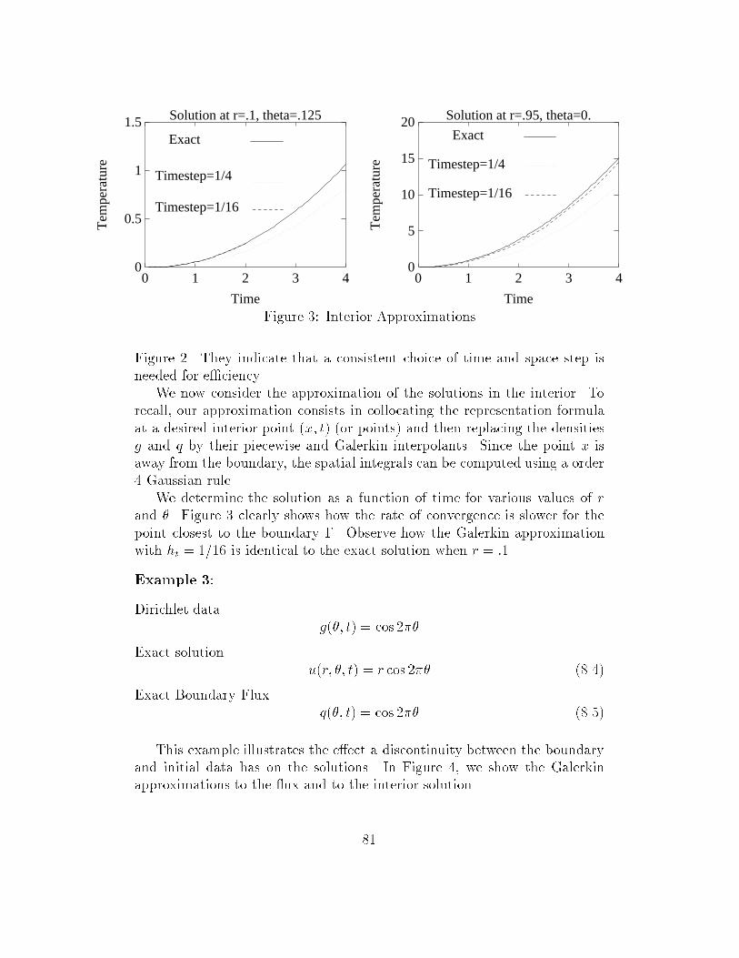
0
0.5
1
1.5
0 1 2 3 4
Time
Tem
pera
ture
Solution at r=.1, theta=.125
Exact
Timestep=1/4
Timestep=1/16
0
5
10
15
20
0 1 2 3 4
Time
Tem
pera
ture
Solution at r=.95, theta=0.
Exact
Timestep=1/4
Timestep=1/16
Figure �� Interior Approximations
Figure �� They indicate that a consistent choice of time and space step isneeded for e�ciency�
We now consider the approximation of the solutions in the interior� Torecall� our approximation consists in collocating the representation formulaat a desired interior point �x� t� �or points� and then replacing the densitiesg and q by their piecewise and Galerkin interpolants� Since the point x isaway from the boundary� the spatial integrals can be computed using a order� Gaussian rule�
We determine the solution as a function of time for various values of rand � Figure � clearly shows how the rate of convergence is slower for thepoint closest to the boundary �� Observe how the Galerkin approximationwith ht � ��� is identical to the exact solution when r � ���
Example ��
Dirichlet datag�� t� � cos ��
Exact solutionu�r� � t� � r cos �� �����
Exact Boundary Fluxq�� t� � cos �� ����
This example illustrates the e�ect a discontinuity between the boundaryand initial data has on the solutions� In Figure �� we show the Galerkinapproximations to the �ux and to the interior solution�
��

0
1
2
3
4
5
0 0.1 0.2 0.3 0.4 0.5 0.6 0.7 0.8 0.9 1
*
*
** * * * * * *
o
o
oo o o o o o o
x
x
xx x
Time
Flux
Timestep 1/5 Spacestep 1/8 x
Timestep 1/10 Spacestep 1/16 o
Timestep 1/10 Spacestep 1/8 *
Approximations to the flux. theta=0.
0
0.2
0.4
0.6
0.8
1
0 0.1 0.2 0.3 0.4 0.5 0.6 0.7 0.8 0.9 1*
*
* * * * * * * * *
.
.
. . . . . . . . .
o
o
o o o o o o o o o
x
x x x x x
Time
Tem
pera
ture
Timestep 1/5 Spacestep 1/8 x
Timestep 1/10 Spacestep 1/8 *
Timestep 1/10 Spacestep 1/16 o
Approximations to the temperature at r=1/2, theta=0.
Figure �� Galerkin Approximations
Clearly� the method behaves quite poorly near the origin t � �� For tunately� however� the e�ect of this discontinuity decays fairly rapidly withtime� Indeed� away from the origin� we found the method to be convergingoptimally�
Example �� In this example� we consider an exterior problem� It is forsuch exterior problems that the boundary element method seems to be mostuseful� We take the boundary � to be the ellipse
E� ��
�x� y� �
x�
x���y�
y��� �
��
with �x�� y�� � ����� ���
��

0
0.1
0.2
0.3
0.4
0.5
0.6
0.7
0.8
0.9
1
0 0.1 0.2 0.3 0.4 0.5 0.6 0.7 0.8 0.9 1
x
x
x
x
x
*
*
*
*
*
*
*
*
*
*
o
o
o
o
o
o
o
o
oo
Time
Flux
Timestep 1/5 Spacestep 1/8 x
Timestep 1/10 Spacestep 1/8 *
Timestep 1/10 Spacestep 1/16 o
Approximations to the flux for theta=0.
Figure � Galerkin Approximation to Flux
In order to have a problem with a known solution� we choose the Dirichletg so that the exact solution u to the heat equation in the exterior is thefundamental solution
u�x� t� �exp��jxj���t�
�t� x � R�� t � ��
Note that g has both a spatial and time dependence since the radius ��� ofE� is
��� �nx�� cos
� �� � y�� sin� ��
o���� ����
It is easy to check that the exact Neumann �ux is
q�� t� �exp��������t�
�t�hx�� sin
������ � y�� cos������i��� �
��

0
0.05
0.1
0.15
0.2
0.25
0.3
0.35
0.4
0.45
0.5
0 0.1 0.2 0.3 0.4 0.5 0.6 0.7 0.8 0.9 1x
x
x
x x
x
**
*
*
*
* * **
**
o o
o
o
o
oo o o
oo
Time
Tem
pera
ture
Approximations to the temperature at r=1.6, theta=0.
Timestep 1/5 Spacestep 1/8 x
Timestep 1/10 Spacestep 1/8 *
Timestep 1/10 Spacestep 1/16 o
Figure � Galerkin Approximation to Solutions
In Figure � we consider the Galerkin approximations to the �ux� Theresults indicate that its spatial step which is controlling the error� The sameremarks can be made about the approximations of the solution� Some ofthese are shown in Figure �
We conclude with some observations� In the �rst example� we saw evi dence that the Galerkin method when applied to smooth functions not onlyconverges optimally in L� by also exhibits superconvergence at the midpoints�In the second example� we saw the competitive e�ect of the discretizations inspace and time� In the third example� we examined how the Galerkin methodbehaves when applied to a problem with incompatible Dirichlet and initialdata� Very encouragingly� we saw that although it behaves quite poorly nearthe discontinuity� the Galerkin method damps out its e�ects fairly rapidly�Lastly� we applied the method to an exterior problem to show how the bound ary element is well suited to such problems�
��
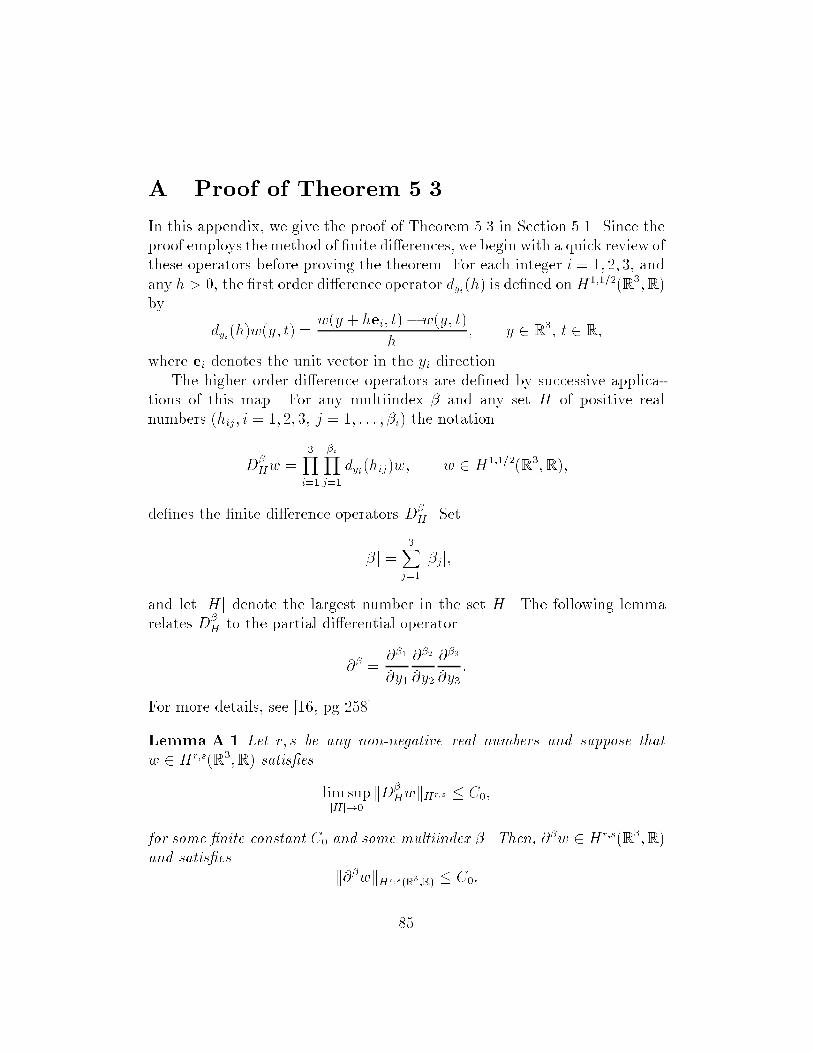
A Proof of Theorem ��
In this appendix� we give the proof of Theorem �� in Section ��� Since theproof employs the method of �nite di�erences� we begin with a quick review ofthese operators before proving the theorem� For each integer i � �� �� �� andany h � �� the �rst order di�erence operator dyi�h� is de�ned onH������R��R�by
dyi�h�w�y� t� �w�y � hei� t�� w�y� t�
h� y � R�� t � R�
where ei denotes the unit vector in the yi direction�The higher order di�erence operators are de�ned by successive applica
tions of this map� For any multiindex � and any set H of positive realnumbers �hij� i � �� �� �� j � �� � � � � �i� the notation
D�Hw �
�Yi��
�iYj��
dyi�hij�w� w � H������R��R��
de�nes the �nite di�erence operators D�H � Set
j�j ��X
j��
j�jj�
and let jHj denote the largest number in the set H� The following lemmarelates D�
H to the partial di�erential operator
�� ����
�y�
���
�y�
���
�y��
For more details� see ��� pg ����
Lemma A�� Let r� s be any non�negative real numbers and suppose thatw � Hr�s�R��R� satis�es
lim supjHj��
kD�HwkHr�s � C��
for some �nite constant C� and some multiindex �� Then� ��w � Hr�s�R��R�and satis�es
k��wkHr�s�R��R� � C��
�

We note some properties satis�ed by the di�erence operators� If denotesthe restriction operator� �i�e��
w�y�� y�� t� � w�y�� y�� �� t�� �y� t� � R� �R� �and � � ���� ��� ��� any multiindex such that �� � �� then
D�Hw�y�� y�� y�� t� � D�
Hw�y�� y�� t��
Another useful property of the �nite di�erence operator is that it commuteswith di�erentiation� i�e�
D�H�
�w � ��D�Hw� for any multiindices �� ��
for w � S�R� � R�� say� Finally� by a simple change of variables� it is easyto prove the important equalityZ �
��
ZR�D�Hw�y� t�v�y� t�dydt � ����j�j
ZR�w�y� t�D�
�Hv�y� t�dydt�
for all w� v � L��R� �R�� �A���
We are now ready to begin the proof� First� we remind the reader of someprevious notation�
# � Heat operator W����� �W��������
� Trace operator W � H��������� �R��Y � fy � R�� jyij � �� i � �� �� �g�Y� � fy � Y � y� � �g�O � An open set in R�� A representative
of the sets in a �nite covering of ��
� � Isomorphism from O � Y �
Here is what we want to prove� Given m � N and q � Hm�����m�������R��let
wq�y� t� � ����uq��y� t�� y � Y � t � R�Theorem �� states that all of the partial derivatives ��wq exist and belongto L��R�H��Y �� so long as j�j � m and �� � �� Moreover� they each satisfyan inequality of the form
k��wqkH������Y�R� � CkqkHm�����m���������R�� �A���
�

Proof of Theorem ���� Let H������ �Y�R� denote the closure of D�Y � R�
in the H������Y�R� norm� �In other words� functions with compact support
in Y �R�� De�ne A� H������ �Y�R��H
������� �Y�R�� C by
A�w� v� � h#���w�� ���v�i � �A���
It is simple to check that A can be written in the form
A�w� v� �Z �
��
ZYi�F t�w��y� � �F t�v��y� � �J�y�dyd�
��Xi�j
Z �
��
ZYaij�y�
�w
�yi�y� t�
�v
�yj�y� t�J�y�dydt� �A���
for each w� v � H������Y�R�� where J�y� denotes the Jacobian of � and whereai�j�y� � C��Y � with the matrix of coe�cients fai�j�y�g being uniformly pos itive de�nite� �That is� there exists a positive constant c which is independentof y � Y such that
�Xi�j
�iai�j�y��j � c�Xi��
��i for all � � R��� �A��
Consequently� there exists some positive constant c such that
A�w� �I �H�w� � ckwk�H������Y�R� for all w � H������� �Y�R�� �A��
where H� H������ �Y�R�� H
������ �Y�R� denotes the Hilbert transform�
We substitute wq for w in �A���� Using the product rule� we get
A�wq� v� � h#uq� ����v�i�Z �
��
ZR�uq�x� t�r��x�r�� �v� �x� t�dxdt
�Z �
��
ZR��� �v� �x� t�r��x�ruq�x� t�dxdt�
where uq � #���q� Hence�
A�wq� v� � h�q� ��� �v�i �Z �
��
ZR�uq�x� t�r��x�r�� �v� �x� t�dxdt
�Z �
��
ZR��� �v� �x� t�r��x�ruq�x� t�dxdt� �A���
��

for all v � H������ �Y�R��
To estimate D�Hwq� we will consider the pairing A�D�
Hwq� v�� Before wecan take this step� however� we must verify that this pairing makes sense forall multiindices � such that j�j � m� Fortunately� this only requires a carefulchoice of the set H so that jHj is su�ciently small� To be precise� let r � �be such that
supp wq��� t� � Yr �� fy � R�� jyij � r� i � �� �� �g � Y�
uniformly with respect to t � R� �The de�nition of wq shows that such an rexists�� Set
�� ��
��
�
�r� and �� �
�
��
�
�r�
so that r � �� � �� � �� Then� it is easy to check that D�Hwq has support
in the set Y�� for all sets H which satisfy
jHj � �
�m��� r��
Moreover� we haveD��HD
�Hwq � H
������ �Y�� �R��
which we will need later�Let v � H
������ �Y�R� be given� Without loss of generality� we choose v so
that its support lies in the cylinder Y�� �R� �This ensures the inclusion
D�Hv � H
������ �Y�R� for any multiindex ���
We now consider the pairing A�D�Hwq� v�� By �A��� and �A���� we have
A�D�Hwq� v� � ����j�jA�wq�D
��Hv� � E��wq� v�� �A���
where
E��wq� v� ��Yl��
�lYk��
�Xi�j
Z �
��
ZY
�wq
�yi�y� t�
�v
�yj�y � hlk� t�D
l�hlkai�j�y�dydt
��Yl��
�jYk��
Z �
��
ZYi�F t�wq��y� � �F t�v��y � hlk� � �D
l�hlk �J�y��dyd��
��

Using �A���� we obtain
A�D�Hwq� v� �
D�q� ���
�D��Hv
�E� E��wq� v� � E��uq� �
��v��� �A���
where
E��uq� ���v�� �
Z �
��
ZR�uq�x� t�r��x�rv���x�� t�dxdt
�Z �
��
ZR�v���x�� t�r��x�ruq�x� t�dxdt�
We now bound the terms E�� and E�� We have
jE��wq� v�j � CkwqkH������Y�R� kvkH������Y�R�� �A����
and
jE��uq� v�j � Cnk����uqkL��R��R� � k jruqj kL��R��R�
okvkH����Y�R�
� CkuqkW�����kvkH������Y�R�� �A����
�To get the last estimate� note that �� � D�R�� and apply Lemma �����Collecting together equations �A���A����� it follows that
A�D�Hwq� v� �
Dq� ���
�D��Hv
�E� E�v�� v � H������Y�� �R�� �A����
where E satis�es
jE�v�j � CnkuqkW����� � kwqkH������Y�R�
okvkH������Y�R�
� CkqkH������������R�kvkH������Y�R�� �A����
To proceed further� we now rewrite the term
Iq ��D�q� ���
�D��Hv
�E�A����
in a form where D��H acts not on v but instead on ����q�� Set
V ��H �y
�� y�� t� � D��H �v� �y�� y�� t�� �y�� y�� t� � Y �R�
Then� from �A����� we have
Iq �Z �
��
Z��O
q�x� t���x�V ��H���x�� t�dxdt�
��
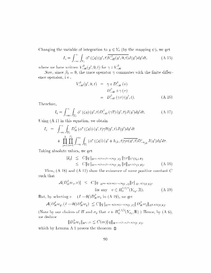
Changing the variable of integration to y � Y� �by the mapping ��� we get
Iq �Z �
��
ZY��� ��q� �y�� t�V �
�H�y�� �� t�J�y��dy�dt� �A���
where we have written V ��H�y
�� �� t� for � V ��H �
Now� since �� � �� the trace operator commutes with the �nite di�er ence operator� i�e��
V ��H�y
�� �� t� � �D��H �v�
� D��H � �v�
� D��H �v� �y�� t�� �A���
Therefore�
Iq �Z �
��
ZY��� ��q� �y�� t�D�
�H �v� �y�� t�J�y��dy�dt� �A����
Using �A��� in this equation� we obtain
Iq �Z �
��
ZY�D�H ��� ��q�� �y�� t�v�y�� t�J�y��dy�dt
��Y
j��
�jYk��
Z �
��
ZY���� ��q�� �y� � hjk� t�v�y�� t�D
j�hjkJ�y
��dy�d��
Taking absolute values� we get
jIqj � CkqkHm�����m���������R� kvkL��Y��R�� CkqkHm�����m���������R� kvkH������Y�R�� �A����
Thus� �A���� and �A���� show the existence of some positive constant Csuch that
jA�D�Hwq� v�j � CkqkHm�����m���������R�kvkH������Y�R��
for any v � H������ �Y���R�� �A����
But� by selecting v � �I �H�D�Hwq in �A����� we get
jA�D�Hwq� �I �H�D�
Hwq�j � CkqkHm�����m���������R�kD�HwqkH������Y�R��
�Note by our choices of H and �� that v � H������ �Y�� �R��� Hence� by �A���
we deducekD�
HwqkH����� � C�m�kqkHm�����m���������R��
which by Lemma A�� proves the theorem�
��

B Proof of Theorem ��
In this appendix� we give the proof of Theorem ��� To recall� we must showthat the solution u to the Dirichlet problem
�u
�t��u � � on R
�n� �R�u � g on ��R�
satis�es the interior and exterior estimates
kukHm���m��������R� � CkgkHm�����m���������R� for each m � N� �B���
and
kukWm���m�������c�R� � CkgkHm�����m���������R� for each m � N� �B���
Observe that the regularity estimates �B���B��� do not say anythingabout the solution u over R� � R� Therefore� we can separately study theDirichlet problem over the interior � � R and the exterior �c � R� We willconcentrate on the exterior problem
�u
�t��u � � on �c �R� �B���
u � g on ��R� �B���
The proof will use localization� Henceforth� we �x m � N and g �Hm�����m���������R�� For convenience� we will write
kgkm�� � kgkHm�����m���������R�� �B��
Continuing with previous notation� let �Oj� �j� �j�M� denote a chart of ��We append to this chart an interior set O� such that O�� O��� � �� OM covers�� and a function �� � D�O�� such that f�j�x�gM� forms a partition of unitywith respect to this cover� We then set
OM�� � R�n
M�j��
Oj�
��

and de�ne
�M���x� � ��MXj��
�j�x�� x � R��
�Again� note that the functions f�j�x�gM��� form a partition of unity over
R���Now� let u denote the solution to �B���B���� To study u� we will consider
each of the functions �ju� for integers j between � and M � �� They areconnected by
u�x� t� �M��Xj��
�j�x�u�x� t�� x � �c� t � R� �B��
To estimate the functions �ju� we shall use a standard inductive argument�Speci�cally� assume that the solution u to �B��� satis�es
u � Wk�k����c�R�� �B���
for some k � N with k � m� We will then show that each �ju satis�es
k�jukWk���k�������c�R� � Cnkgkm�� � kukWk�k���c�R�
o� �B���
Clearly� because of �B��� equation �B��� implies that
kukWk���k�������c�R� � Cnkgkm�� � kukWk�k���c�R�
o� �B���
for any k � N with k � m� Noting that �B��� is true for k � �� induction onk in �B��� shows that
kukWm���m�������c�R� � Ckgkm�� for any m � N� �B����
The estimates �B��� will be proven based the di�erential equation
#��ju��x� t� � �ru�x� t�r�j�x��u�x� t���j�x�� �x� t� � �c�R� �B����
�ju�x� t� �
�j�x�g�x� t� j � �� �� � � �M� j � M � �
� x � �� t � R�
solved by �ju� In the next theorem� we show �B��� for j � M � ��
��

Theorem B�� For any integer k � N� let u � Wk�k����c�R� satisfy
#u�x� t� � �� x � �c� t � R� �B����
and let �x� � D�R�� satisfy �x� � � on ��� Then� there exists a positiveconstant C which depends only on k and such that
k��� �ukWk���k�������c�R� � CkukWk�k���c�R�� �B����
Proof� We apply the heat operator # to ��� �u� We get
#�� � �u � �� � �#u� F
� F� �by �B������ �B����
where
F �x� t� � �ru�x� t�r�x� � u�x� t���x�� x � �c� t � R�
Since � � on ��� it follows that F � � on ���R� Because ��� �u alsovanishes over this set� we can extend both sides of equation �B���� by zeroto ��� We get
#��� ��x� t� � F �x� t�� x � R�� t � R�
To conclude the proof� we will verify the inclusion
F �x� t� � Hk���k�������R��R� W�������� �B���
and apply Theorem �� �This theorem showed that
# �Wk���k������ � Hk���k�������R��R� W��������
is an isomorphism�� The main observation to showing �B��� is to note thatthe support of F �x� t� is contained in some cylinder BR�R of �nite radius R�It is easily checked that any Hk���k�������R��R� function which is supportedin this fashion also belongs to W��������
Hence� we must verify that
�rur� u� � Hk���k�������R��R�� �B���
��

But� by de�nition ofWk�k����c�R�� we have the existence of positive constantC� such that
k jruj kHk���k�������c�R� � C�kukWk�k���c�R�� u � Wk�k����c�R��
Similarly� since Wk�k����c�R� and Hk�k����c�R� di�er only in their behaviornear in�nity� it follows that there exists a positive constant C��� such that
ku�kHk�k���R��R� � C��kukWk�k���c�R��
Hence� �B��� holds�
It remains to consider �B���� for the indices j which lie between � andM � Since the supports of the functions �ju are bounded in this case� we add�ju to each side of �B����� We get
#��ju� � �ju � Fj�x� t�� �x� t� � �c �R��ju � �jg�x� t�� �x� t� � ��R� �B����
where
Fj�x� t� � ��ru�x� t�r�j�x�� u�x� t���j�x� � �j�x�u�x� t��
�x� t� � �c �R� j � �� � � � �M�
The way to study the parabolic problems represented in �B���� is to mapthem into equivalent problems which are posed over the half space Y� �R�where
Y� � f�y�� y�� y��� jyij � �� i � �� �� � � y� � �g�Before we do this� it is convenient to reduce �B���� to an equivalent Dirichletproblem with homogeneous boundary condition� Let ug�x� t� � Wm���m������
denote any extension of g such that
ug�x� t� � g�x� t�� �x� t� � � �R�We then de�ne Uj � �ju� �jug� This function satis�es
#�Uj� � Uj � fj�x� t�� �x� t� � R� �R�Uj � �� �x� t� � ��R� �B����
wherefj�x� t� � Fj�x� t�� # ��jug� �x� t�� �x� t� � �c �R�
��

To map �B���� to the half space Y� �R� let
wj�y� t� � ��j �Uj��y� t�� �y� t� � Y� �R�
This leads to
wj
t�y� t�� Lwj�y� t� � wj�y� t� � ��j �fj��y� t�� �y� t� � Y� �R�
wj�y� t� � �� �y� t� � Y� �R��B����
where L denotes the uniformly strongly elliptic di�erential operator
Lw�y� t� ��X
i�j��
ai�j�y���w
�yi�yj�y� t�� �y� t� � Y �R�
�In particular� the matrix of coe�cients fai�j�y�g is positive de�nite� uni formly for y � Y �� Let
L�w�y� t� ��X
i�j��
ai�j�����w
�yi�yj� �y� t� � Y� �R�� �B����
The mapping properties of the parabolic operator I�#� �� ���t�L��Iare well understood ��� Chapter ��� We state them in a lemma�
Lemma B�� For each k � N� let Hk���k������� �Y��R� denote the closure of
D�Y��R� in the Hk���k�������Y��R� norm� For any f � Hk���k������� �Y��R��
there exists a unique solution w � Hk���k������� �Y��R� to
�w
�t� L�w � w � f on Y� �R� �B����
w � � on Y� �R� �B����
which satis�es
kwkHk���k�������Y��R� � C�k�kfkHk���k�������Y� �R��
Set #� � ���t� L� and let L� � L� L�� so that
�
�t� L� I � �#� � I� � L��
�

To deduce the mapping properties of the operator I�#��L�� we shall showthat the operator L� amounts in some sense to a small perturbation of theoperator I � #�� The next theorem is the crucial step� For brevity� we shallhenceforth use the abbreviations
kukk�Y��R� kukHk�k���Y� �R�� and kukk�R���R� kukHk�k���R���R�� k �Z�
Theorem B�� Let k � N and f � Hk�k��� �Y��R�� Given any � � �� there ex�
ists some � � � which depends on � and k but not on f � such that supp f � B� �Rimplies that
kL��I � #����fkk�Y��R� �kfkk�Y��R� �B����
We of course mean �I � #���� in the sense of Lemma B��� We postponethe proof for the moment to show how we will use it� Set
zj � �I � #���ju�
and by �B����� we havehI � L��I � #��
��i zj � ��j �fj� �
and thus
khI � L��I � #��
��i zjkk���Y� �R� � k��j�fj�kk�Y��R�� CkfjkWk�k���c�R�
� CkukWk���k�������c�R�� �B����
Now� by Lemma B���
k�jukWk���k�������c�R�
� C��k�kzjkk���R��R� k � N� �B���
Since the support of the cuto�s functions �j may be chosen su�ciently smalland because
supp zj � supp� �ju��
we may apply Theorem B�� and the triangle inequality in �B���� to deducethe existence of some positive constant C� which depends on k and �j suchthat
kzjkk�Y��R� C� k �I � L��I � #�����zj kk�Y��R�
Combining this with �B��� yields the desired inequality
k�jukWk���k�����c�R� � C�k�kukWk���k�������c�R��
�

It remains to prove Theorem B��� We need two lemmas� In these lemmas�we use the notation
B�� � fy � �y�� y�� y�� � R�
� � y� � �� jyj � �g� � � ��
Lemma B�� Let k � N and � Hk���R���� Given any � � �� there exists
some � � � which depends on � and k but not on � such that supp � B��
implies thatkkHk�R���
� �kkHk���R����
We refer the reader to ���� p� �� for the proof and state an importantcorollary to this result�
Corollary B�� Let k � N and � Hk���k�������R���R�� Given any � � ��
there exists some � � � which depends on � and k but not on � such thatsupp � B�
� �R implies that
kkHk�k���R���R�� �kkHk���k�������R���R�
� �B���
Proof� Let � � �� k � N� and � Hk�k���R���R� be given� The key to the
corollary is to note by interpolation theory that there exists some positiveconstant C� such that
kkHk���R�H��R����� C�kkHk���k�������R�� �R�
� k � N�
Now� by Lemma B��� there exists some �� � � such that
kkL��R�Hk�R����� �
�C�kkL��R�Hk���R����
�
if the support of is contained in B���� R� Analogously� there exists some
�� � � such that
kkHk���R�L��R����� �
�C�kkHk���R�H��R����
� k � N�
if the support of is contained in B����R� The corollary follows by setting
� � min���� ��� and restricting the support of to lie in B�� �R�
��

Lemma B�� Let k � N and � Hk���k�����R���R�� Given any � � ��
there exists some � � � which depends on k and � but not on � such thatsupp � B�
� �R implies that
kL�kk�R���R� �kkk���R���R �B����
Proof� Fix k � N and let � Hk���k�������R��R� be given� Without lossof generality� we can assume that the support of is contained in the halfcylinder B�
� �R for some � � � � �� From the de�nition of the operator L��we shall derive two inequalities�
First� by direct di�erentiation and the product rule� there exists a positiveconstant C��k� such that
kL�kL��R�Hk�R�����
maxi�j
kai�j�y�� ai�j���kL��B�� �
�kkL��R�Hk���R����
� C��k�kkL��R�Hk���R���� �B����
Analogously� we have
kL�kHk���R�L��R������maxi�j
kai�j�y�� ai�j���kL��B�� �
�kkHk���R�H��R����
�
SincekkHk���R�H��R����
� C��k�kkk���R���R�by interpolation theory� we have
kL�kHk���R�L��R����� C��k�
�maxi�j
kai�j�y�� ai�j���kL��B�� �
�kkk���R���R�
�B����Hence� by combining �B����B����� we have
kL�kk�R���R � C��k� �
maxi�j
kai�j�y�� ai�j���kL��B���
�kkk���R���R
� kkk���R���R�� �B����
for some positive constant C��k��Now� the continuity of the coe�cients ai�j implies that for any given � � ��
there exists some �� � � such that
C��k� maxi�j
kai�j�y�� ai�j���kL��B����
�� �
�� �B����
��

Analogously� by Corollary B�� there exists some �� � � such that
C��k�kkk���R���R��
�kkk���R���R� �B����
for all supported in B����R� The lemma follows by combining �B���� with
�B���� and choosing � � min���� ����
Proof of Theorem B�� � Fix k � N and let f � Hk�k��� �Y��R� have
support contained in B�� � R for some � � � � �� Choose any � � D�Y��
with � � � on the support of f � We shall now show the existence of somepositive constant C� which depends on k and � but not on f � such that
k�� � ���I � #����fkk���Y��R� C���� k�kfkk�Y�R� �B����
Note that it is the di�erence of � between the subscripts of the norms asopposed to � which makes this a non trivial statement�
To prove it� observe that
�I � #����� ���I � #����f � f � �I � #����I � #��
��f
� �f � �f� �G�
whereG � �f � �I � #����I � #��
��f�
But� since � equals one on the support of f � it follows that
�I � #���� � ���I � #����f � G� �B����
Now� set w� � �I � #����f � Because
�I � #���w� � ��I � #��w� �Xi�j
ai�j����w�
�yi
��
�yj
�Xi�j
ai�j���w����
�yi�yj�
it follows that
G�y� t� �X
ai�j����w�
�yi
��
�yj
�Xi�j
ai�j���w��y� t����
�yi�yj�
��

for each �y� t� � Y� �R� Hence�
kGkk�Y��R� C���� k�kw�kk���Y� �R� �B���
We now applying the operator �I �#���� to both sides of �B����� Doingthis and then taking norms� we get
k�� � ��I � #����fkk���Y��R � k�I � #��
��Gkk���Y��R� C��k�kGkk���Y� �R� C���� k�k�I � #��
��fkk���Y� �R� C���� k�kfkk�Y��R� �B���
which veri�es �B�����To complete the proof� let �� and �� denote two positive numbers to be
determined� To estimate L��I � #����f � write
L��I � #����f � L���� ���I � #��
��f � L���I � #����f�
and take norms� This yields
kL��I � #����fkk�Y� �R � kL���� ���I � #��
��fkk�Y��R� kL���I � #��
��fkk�Y��R� C��k�k��� ���I � #��
��fkk���Y� �R� kL��I � #��
��fkk���Y��R�We �rst apply Lemma B� to this inequality to get
kL��I � #����fkk�Y� �R � C��k�k��� ���I � #��
��fkk���Y� �R� ��k��I � #��
��fkk���Y��R� �B����
By then using
k��I � #����fkk���Y��R � k�I � #��
��fkk���Y��R� k�� � ���I � #��
��fkk���Y��R�in �B����� we have
kL��I � #����fkk�Y��R � �C��k� � ���k��� ���I � #��
��fkk���Y��R� ��k�I � #��
��fkk���Y� �R�
���

To conclude� apply �B���� to this equation to get
kL��I � #����fkk�Y��R � C��k��C��k� � ���kfkk���Y��R
� ��k�I � #����fkk���Y� �R
� C��k��C��k� � ���kfkk���Y��R� ��C��k�kfkk�Y��R�
and then apply �B��� to the �rst term to deduce
kL��I � #����fkk�Y��R� C�k� �����kfkk�Y��R� �B����
whereC � ��C��k��C��k� � ��� � ��C��k��
Clearly� this implies the theorem�
���

C Solutions to the Heat Equation Over the
Unit Circle
In this appendix� we describe how to solve the heat equation
�u
�t�x� t���u�x� t� � �� x � B�� t � ��
u�x� �� � �� x � B�� �C����
u�x� t� � g�x� t�� x � �B�� t � ��
in the unit disk B�� Again� we will describe the points of B� by polar coor dinates �r� � with scaled to lie between � and �� For simplicity� we shallassume that g��� �� � ��
The �rst step is transform to a Dirichlet problem where the inhomoge neous condition appears as a forcing function� This is done by letting "g�r� � t�denote any extension of the Dirichlet data g to the interior of the circle andthen letting U � u� "g� Though "g is obviously non unique� the best choiceappears to be an harmonic extension� In other words� we choose "g so that
�"g�r� � t� � �� r � �� � ��� ��� t � ��
"g��� � t� � g�� t�� � ��� ��� t � ��
With this choice of "g� we �nd that U satis�es the inhomogeneous equation
�U
�t�r� � t���U�r� � t� � ��"g
�t�r� � t�� r � �� � ��� ��� t � �� �C����
with homogeneous initial and boundary conditions�Problem �C���� is now in the form where Duhamel�s principle �cf�� ���� p�
���� applies� For each s � �� let v�r� � t% s� denote the solution to
�v
�t�r� � t% s��v�r� � t% s� � �� t � s�
v��� � t% s� � �� t � s� �C����
v�r� � s% s� � ��"g�t
�r� � t��
Note that the variable s in �C���� represents the initial time and is viewed asa parameter� Duhamel�s principle states that the solution to �C���� is given
���

by
U�r� � t� �Z t
�v�r� � t% s�ds�
Of course� the transformations used to get to �C���� apply for any prob lem� not simply ones over the unit circle� The reason why the circle is specialis that �C���� can be solved using separation of variables� The general formof the solution v is
v�r� � t% s� ��X
m���
�Xk��
Ak�m�s�Jm��m�kr�e���m�kteim�� �C����
where �m�k are the roots of
Jm��m�k� � �� m �Z� k �Z��
and Ak�m�s� the so called Fourier Bessel coe�cients which are determined by
��g�t
�r� � s� ��X
m���
�Xk��
Ak�m�s�Jm��m�kr�e���m�kseim��
Thus�
Ak�m �
R ���
R �� rFg�r� � s�Jm��m�kr� drdR �
� r �Jm��m�kr��� dr
�
where we have set Fg � ��g��t�Remark� To compute the series in �C����� the various identities found in ���p� ���� such as
�Xk��
�
��m�k
��
��m� ���
and �Xm��
�
��m�k
��
��m� ����m� ��� m � Z��
were found to be quite useful�
���
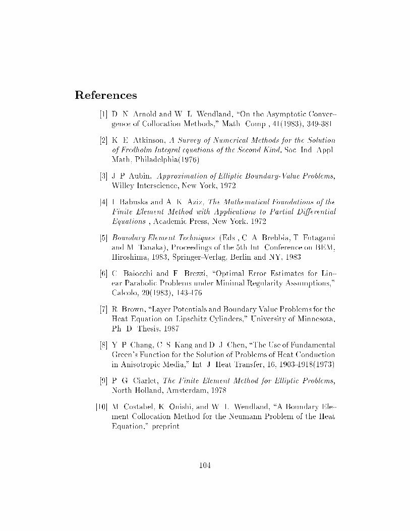
References
��� D� N� Arnold and W� L� Wendland� *On the Asymptotic Conver gence of Collocation Methods�+ Math� Comp�� ��������� ��� ����
��� K� E� Atkinson� A Survey of Numerical Methods for the Solutionof Fredholm Integral equations of the Second Kind� Soc� Ind� Appl�Math� Philadelphia������
��� J� P� Aubin� Approximation of Elliptic Boundary�Value Problems�Willey Interscience� New York� �����
��� I� Babuska and A� K� Aziz� The Mathematical Foundations of theFinite Element Method with Applications to Partial Di�erentialEquations � Academic Press� New York� �����
�� Boundary Element Techniques �Eds�� C� A� Brebbia� T� Futagamiand M� Tanaka�� Proceedings of the th Int� Conference on BEM�Hiroshima� ����� Springer Verlag� Berlin and NY� �����
�� C� Baiocchi and F� Brezzi� *Optimal Error Estimates for Lin ear Parabolic Problems under Minimal Regularity Assumptions�+Calcolo� ��������� ��� ���
��� R� Brown� *Layer Potentials and Boundary Value Problems for theHeat Equation on Lipschitz Cylinders�+ University of Minnesota�Ph� D� Thesis� �����
��� Y� P� Chang� C� S� Kang and D� J� Chen� *The Use of FundamentalGreen�s Function for the Solution of Problems of Heat Conductionin Anisotropic Media�+ Int� J� Heat Transfer� �� ���� ����������
��� P� G� Ciarlet� The Finite Element Method for Elliptic Problems�North Holland� Amsterdam� �����
���� M� Costabel� K� Onishi� and W� L� Wendland� *A Boundary Ele ment Collocation Method for the Neumann Problem of the HeatEquation�+ preprint�
���

���� D� Curran� M� Cross� and B� A� Lewis� *A Preliminary Analysisof Boundary Element Methods Applied to Parabolic Partial Dif ferential Equations�+ in New Developments in Boundary ElementMethods �C� A� Brebbia� ed��� CML Publications� Southhampton������
���� D� Curran and B� A� Lewis� *A Boundary ElementMethod for theSolution of the Transient Di�usion Equation in Two Dimensions�+Appl� Math� Modelling� �������� ��� ����
���� J� Deny and J� L� Lions� *Les Espaces de Type Beppo Levi�+ Ann�Inst� Fourier� ���� ����� �� ����
���� E� B� Fabes and N� M� Riviere� * Dirichlet and Neumann Problemsfor the Heat Equation in C� Cylinders�+ Proceedings of Symposiain Pure Mathematics� Vol� XXXV� Part � ������� ��� ���
��� G� Fairweather� F� J� Rizzo and D� J� Shippy� *Computation ofDouble Integrals in the Boundary Integral Equation Method�+ inAdvances in Computer Methods for Partial Di�erential EquationsIII� R� Vichnevetsky and R� S� Stepleman� eds�� New Brunswick�IMACS� ����� ��� ����
��� G� B� Folland� Introduction to Partial Di�erential Equations�Princeton University Press� Princeton� NJ� ����
���� A�Friedman� Partial Di�erential Equations of Parabolic Type �Prentice Hall� Englewood Cli�� NJ �����
���� M� Gevrey� Sur les Equations Aux Derivees Partielles du TypeParabolique�+ Journal de Math�� Ser� � Vol� �� ����� pp� �� ����
���� J� Giroire and J� C� Nedelec� *Numerical Solution of an Exte rior Neumann Problem Using a Double Layer Potential� Math� ofComp�� ������������ ����
���� B� Hanouzet� *Espaces de Sobolev Avec Poids� Application auproblem de Dirichlet dans un demi space�+ Rendiconti del Semi nario Matematico dell�Universit,a di Padova� XLVI������� ��� ����
��

���� E� Holmgren� *Sur une Application de l�Equation Integrale de M�Volterra�+ Ark� Mat� Astronom� Fys�� Vol� �� ����� � ��
���� S� Kaplan� *Abstract Boundary Value Problems for LinearParabolic Equations�+ Ann� Scuola� Norm� Sup� Pisa� ��������� ����
���� J� L� Lions� Equations Di�erentielles Operationelles et ProblemsAux Limits� Springer Verlag� Berlin� ����
���� J� L� Lions and E� Magnes� Problems Aux Limites non Homoge�nous et Applications � Vol��� Dunod� Paris� ����
��� J� L� Lions and E� Magnes� Problems Aux Limites non Homoge�nous et Applications � Vol��� Dunod� Paris� ����
��� E� A� McIntrye Jr�� *Boundary Integral Solution of the Heat Equa tion�+ Math Comp�� ������� �� ���
���� G� Miranda� *Integral Equation Solution of the First Initial Boundary Value Problem for the Heat Equation in Domainswith Non smooth Boundary�+ Comm� Pure and Appl� Math��XXIII������� �� ��
���� J� C� Nedelec and J� Planchard� * Une Methode Variationalled�Elements Finis Pour la Resolution Numerique d�un ProblemeExterieur dans R��+ Rairo R �� ������� �� ����
���� J� C� Nedelec� *Curved Finite ElementMethods for the Solution ofSingular Integral Equations on Surfaces in R��+ Comput� MethodsAppl� Mech� Engrg� ������� � ���
���� H� Okamoto� *Applications of the Fourier Transform to theBoundary Element Method under the Dirichlet Boundary Con dition�+ preprint�
���� F� W� J� Olver� Asymptotics and Special Functions� AcademicPress� New York� �����
���� K� Onishi� *Convergence in the Boundary Element Method forthe Heat Equation�+ Tru� Math� ��� ��� ���������
��

���� Ozisik� M� N�� Heat Conduction� John Wiley and Sons� New York������
���� H� L� G� Pina and J� L� M� Fernandes� *Applications in TransientHeat Conduction�+ Chapter �� Topics in Boundary Element Re�search� �Ed� C� A� Brebbia �� Vol� �� pp� �� �� Springer Verlag�New York�
��� W� Pogorzelski� Integral Equations � Vol� �� Pergamon Press� Ox ford������
��� W� Pogorzelski� *Sur la Solution de l�Equation Integrale dans leProbleme de Fourier�+ Ann� de la Soc� Polon de Math�� �������� ���
���� W� Pogorzelski� *Sur le Probleme de Fourier Generalise�+ Ann�Polon� Math�� ������ �� ����
���� W� Pogorzelski� *Probleme Aux Limites Pour l�EquationParabolique Normale�+ Ann� Polon� Math�� ������� ��� ���
���� M� N� Le� Roux� *Method D�Elements Finis Pour La ResolutionNumeriqueDe Problems Exterieurs en Dimension ��+ Rairo� Anal�Num�� �������� �� ��
���� W� Rudin� Functional Analysis � McGraw Hill Book Company�New York� �����
���� C� Johnson and L� R� Scott� *An Analysis of Quadrature Errorsin Second Kind Boundary Integral Methods�+Preprint� �����-��
���� F� Sgallari� *A Weak Formulation of Boundary Integral Equationsfor Time Dependent Problems�+ Appl� Math� Modelling� ��������� ����
���� R� P� Shaw� *An Integral Equation Approach to Di�usion�+ Int�J� Heat Transfer� ��������� �� ���
���� F� Treves� Basic Linear Partial Di�erential Equations� AcademicPress� New York� ����
���
��� G� N� Watson� A Treastise on the Bessel Functions� CambridgeUniversity Press� London and New York� �����
��� W� L� Wendland� *Asymptotic Convergence of Boundary ElementMethods�+ in Lectures on the Numerical Solution of Partial Di�er�ential Equations� I� Babuska� T� P� Liu� and J� Osborn� eds��� Lec ture Notes� Vol ���� University of Maryland� College Park� MD������� �� ���
���� L� C� Wrobel and C� Brebbia� *Time Dependent Potential Prob lems�+ in Progress in Boundary Element Methods �
���