Symmetric Galerkin boundary element computation … · Symmetric Galerkin boundary element computation of T-stress ... constraint and fracture toughness ... approach involves one

$Page 1: Symmetric Galerkin boundary element computation … · Symmetric Galerkin boundary element computation of T-stress ... constraint and fracture toughness ... approach involves one$
Symmetric Galerkin boundary element computation of T-stress

and stress intensity factors for mixed-mode cracks

by the interaction integral method

Alok Sutradhar, Glaucio H. Paulino*

Newmark Civil Engineering Laboratory, Department of Civil and Environmental Engineering, University of Illinois

at Urbana-Champaign, MC-250, 205 North Mathews Avenue, Urbana, IL 61801-2352, USA

Received 10 November 2003; revised 17 February 2004; accepted 23 February 2004

Available online 11 June 2004

Abstract

An interaction integral method for evaluating T-stress and mixed-mode stress intensity factors (SIFs) for two-dimensional crack problems

using the symmetric Galerkin boundary element method is presented. By introducing a known auxiliary field solution, the SIFs for both mode

I and mode II are obtained from a path-independent interaction integral entirely based on the Jð; J1Þ integral. The T-stress can be calculated

directly from the interaction integral by simply changing the auxiliary field. The numerical implementation of the interaction integral method

is relatively simple compared to other approaches and the method yields accurate results. A number of numerical examples with available

analytical and numerical solutions are examined to demonstrate the accuracy and efficiency of the method.

q 2004 Elsevier Ltd. All rights reserved.

Keywords: Fracture mechanics; Mixed-mode stress intensity factors; T-stress; Symmetric Galerkin boundary element method; Interaction integral

(M-integral); Two-state integral

1. Introduction

Fracture behaviour is generally characterized by a single

parameter such as the stress intensity factors (SIFs) or path-

independent J-integral [1]. These quantities provide a

measure of the dominant behaviour of the stress field in the

vicinity of a crack-tip. In order to understand the effect of the

structural and loading configuration on the ‘constraint’ [2]

conditions at the crack-tip, another parameter is required. A

second fracture parameter often used is the elastic T-stress. In

two dimensions, the T-stress is defined as a constant stress

acting parallel to the crack and its magnitude is proportional

to the nominal stress in the vicinity of the crack. Various

studies have shown that the T-stress has significant influence

on crack growth direction, crack growth stability, crack-tip

constraint and fracture toughness [3–8]. In order to calculate

the T-stress, researchers have used several techniques such as

the stress substitution method [9], the variational method

[10], the Eshelby J-integral method [11,12], the weight

function method [13], the line spring method [14], the Betti–

Rayleigh reciprocal theorem [15,16], and the interaction

integral method [15,17]. Among these methods, the Eshelby

J-integral method, the Betti–Rayleigh reciprocal theorem

and the interaction integral method are based on path-

independent integrals. In these methods, the fracture

parameters can be calculated using data remote from the

crack-tip and, as a result, higher accuracy compared to local

methods can be achieved.

For a few idealized cases, analytical solutions for

T-stress and SIFs are available. However, for practical

problems involving finite geometries with complex loading,

numerical methods need to be employed. The boundary

element method (BEM) has emerged as a powerful

numerical method for computational fracture analysis. In

BEM analysis, only the boundary of the domain is

discretized and unknown quantities are determined only

on the boundaries. Compared to domain-type methods (e.g.

finite element method (FEM) and meshless methods [18]),

this boundary method significantly reduces the problem size

and the problem setup. Additionally, remeshing of propa-

gating cracks, which only involves local operations on

0955-7997/$ - see front matter q 2004 Elsevier Ltd. All rights reserved.

doi:10.1016/j.enganabound.2004.02.009

Engineering Analysis with Boundary Elements 28 (2004) 1335–1350

www.elsevier.com/locate/enganabound

* Corresponding author. Tel.: þ1-217-333-3817; fax: þ1-217-265-8041.

E-mail address: [email protected] (G.H. Paulino).

http://www.elsevier.com/locate/enganabound

the propagating tip/front region, is simple and easy. The

Galerkin BEM has several advantages over the collocation

BEM. The biggest advantage is that the hypersingular

integrals can be evaluated using standard C0 elements

without any compromise or ambiguity [19]. Moreover, the

weighted averaging formula in the Galerkin BEM provides

a reliable solution in the neighborhood of geometric

discontinuities such as corners and junctions. The Galerkin

approach involves one more integration compared to

collocation. The symmetric Galerkin BEM (SGBEM) uses

both the standard singular displacement boundary integral

equation (BIE) and the hypersingular traction BIE in such a

way that the resultant coefficient matrix for the linear system

becomes symmetric. The symmetry property of the

coefficient matrix reduces the computation time of the

problem. Also by exploiting symmetry [20] and using faster

algorithms [21] in setting up the coefficient matrix,

computational effort can be further reduced. This paper is

based on the SGBEM [22–25], and follows the approach of

Ref. [26]. A recent review [19] provides an excellent

introduction to the literature on the SGBEM.

The interaction integral method is based on conservation

laws of elasticity and fundamental relationships in fracture

mechanics [27]. SIFs pertaining to mixed-mode fracture

problems can be easily obtained from this integral. The basis

of the approach lies in the construction of a conservation

integral for two superimposed states (actual and auxiliary)

of a cracked elastic solid. The analysis requires integration

along a suitably selected path surrounding the crack-tip. The

method was originally proposed by Chen and Shield [27],

and later implemented numerically by Yau et al. [28] using

the FEM applied to homogenous isotropic materials. Since

then, this method has been used by many other researchers.

For instance, Wang et al. [29] applied the method to

anisotropic materials, and Gosz and Moran [30] investigated

three-dimensional (3D) interface cracks. Recently this

method has been widely used to determine mixed-mode

SIFs in functionally graded materials (FGMs). Dolbow and

Gosz [31] originally developed it with the extended FEM

(X-FEM). Rao and Rahman [32] implemented this method

using the element free Galerkin (EFG) method. Kim and

Paulino [33,34] used the method to solve mixed-mode crack

problems in isotropic and orthotopic FGMs in conjunction

with the FEM and micromechanics models. They have

also extended the two-state integral approach to evaluate

T-stress in isotropic [35,36] and orthotopic [37] FGMs.

In the BEM literature, the displacement correlation

technique (DCT) is widely used to evaluate SIFs due to its

simplicity in numerical implementation [38]. Among the

path-independent integral techniques, Aliabadi [39] applied

the J-integral to mixed-mode crack problems by decoupling

the J into its symmetrical and anti-symmetrical portions.

Sladek and Sladek [40] used the conservation integral

method in thermoelasticity problems to calculate the

T-stress, and the J-integral to calculate the SIFs. Denda

[41] implemented the interaction integral for mixed-mode

analysis of multiple cracks in anisotropic solids using a

dislocation and point force approach (Lekhnitskii –

Eshelby–Stroh formalism). Wen and Aliabadi [42] pro-

posed a different contour integral based on Westergaard’s

solution and Betti’s reciprocal theorem to calculate the SIFs.

Reviews of the application of the BEM in fracture can be

found in Refs. [43,44]. In this paper, we develop a unified

scheme by using the interaction integral method for

calculating both the T-stress and the SIFs for mixed-mode

cracks by means of the SGBEM. Recently, Gray et al. [26]

proposed a modified quarter-point element for a more

accurate representation of the crack opening displacement.

The present methodology also includes this improved crack-

tip element.

The remaining sections of this paper are organized as

follows. Section 2 provides the definition of the T-stress.

The interaction integral (called M-integral) method for

calculating the fracture parameters is described in Section 3.

Section 4 gives an introduction to the SGBEM, followed by

the SG formulation for fracture and selected features of the

modified quarter-point element. Section 5 presents various

numerical examples in which the T-stress and the SIFs are

evaluated by means of the M-integral. Finally, Section 6

concludes with some closing remarks and potential exten-

sions. The Appendices A–D supplement the paper.

2. Fracture parameters: T-stress and stress

intensity factors

Williams’ asymptotic solution [45] for crack-tip stress

fields in any linear elastic body is given by a series of the

form

sijðr; uÞ ¼ A1r21=2f ð1Þij ðuÞ þ A2f ð2Þij ðuÞ þ A3r1=2f ð3Þij ðuÞ

þ higher order terms; ð1Þ

where sij is the stress tensor, r and u are polar coordinates

with the origin at the crack-tip as shown in Fig. 1, f ð1Þij ; f ð2Þij ;

f ð3Þij are universal functions of u; and A1; A2; A3 are

parameters proportional to the remotely applied loads. In the

vicinity of the crack ðr ! 0Þ; the leading term which

exhibits a square-root singularity dominates. The amplitude

of the singular stress fields is characterized by the stress

intensity factors (SIFs), i.e.

sij ¼KIffiffiffiffiffi2pr

p f IijðuÞ þ

KIIffiffiffiffiffi2pr

p f IIij ðuÞ; ð2Þ

where KI and KII are the mode I and mode II SIFs,

respectively.

The second term in the Williams’ series solution (Eq. (1))

is a non-singular term, which is defined as the elastic

T-stress. Thus, the above expression (2) can be expanded to

A. Sutradhar, G.H. Paulino / Engineering Analysis with Boundary Elements 28 (2004) 1335–13501336

include this term as follows:

sij ¼KIffiffiffiffiffi2pr

p f IijðuÞ þ

KIIffiffiffiffiffi2pr

p f IIij ðuÞ þ Td1id1j: ð3Þ

The T-stress varies with different crack geometries and

loadings. It plays a dominant role on the shape and size of

the plastic zone, the degree of local crack-tip yielding, and

also in quantifying fracture toughness. For mixed-mode

problems, the T-stress contributes to the tangential stress

and, as a result, it affects the crack growth criteria. By

normalizing the T-stress with the applied load s0ð¼

KI=ffiffiffiffipa

pÞ; a non-dimensional parameter B can be defined

by [2,10]

B ¼ Tffiffiffiffipa

p=KI; ð4Þ

where a is the crack length. The dependence on geometrical

configurations can be best indicated by the biaxiality

parameter B:

3. The two-state interaction integral: M-integral

The interaction integral or M-integral is derived from the

path-independent J-integral [1] for two admissible states of

a cracked elastic FGM body. The formulation of the

M-integral is presented here followed by techniques to

calculate T-stress and SIFs. Finally, some aspects of the

numerical scheme adopted for the implementation of the

contour integral are discussed.

3.1. Basic formulation

The path-independent J-integral [1] is defined as

J ¼ limG!0

ðGðWd1j 2 sijui;1Þnj dG; ð5Þ

where W is the strain energy density given by

W ¼ð1kl

0sij d1ij ð6Þ

and nj denotes the outward normal vector to the contour G;

as shown in Fig. 1.

If two independent admissible fields are considered

where the displacements, strains and stresses of the actual

fields and the auxiliary fields are denoted by ðu;1;sÞ and

ðuaux; 1aux;sauxÞ; respectively, then the J-integral of the

superimposed fields (actual and auxiliary) can be written as:

Js ¼ðG

�1

2ðsik þ saux

ik Þð1ik þ 1auxik Þd1j 2 ðsij þ saux

ij Þ

� ðui;1 þ uauxi;1 Þ

�nj dG: ð7Þ

This integral can be conveniently decomposed into

Js ¼ J þ Jaux þ M; ð8Þ

where J is given by Eq. (5), Jaux is given by

Jaux ¼ðGðWauxd1j 2 saux

ij uauxi;1 Þnj dG ð9Þ

with

Waux ¼ð1aux

kl

0saux

ij d1auxij ; ð10Þ

and M is the interaction integral involving the cross terms of

actual and auxiliary fields, which is given by

M¼ðG

1

2ðsik1

auxik þsaux

ik 1ikÞd1j2ðsijuauxi;1 þsaux

ij ui;1Þ

� �nj dG:

ð11Þ

The M-integral deals with interaction terms only, and will

be used directly for solving mixed-mode fracture mechanics

problems.

3.2. Auxiliary fields for T-stress

The auxiliary fields are judiciously chosen for the

interaction integral depending on the nature of the problem

to be solved. Since the T-stress is a constant stress that is

parallel to the crack, the auxiliary stress and displacement

fields are chosen due to a point force f in the x1 direction

(locally), applied to the tip of a semi-infinite crack in

an infinite homogeneous body, as shown in Fig. 2(a).

Fig. 1. Schematic of integration path and coordinate systems. Notice the

Cartesian ðx1; x2Þ and polar ðr; uÞ coordinate systems at the crack-tip. The

notation �u denotes prescribed displacements and �t denotes prescribed

tractions.

A. Sutradhar, G.H. Paulino / Engineering Analysis with Boundary Elements 28 (2004) 1335–1350 1337

The auxiliary stresses are given by Michell’s solution [46]:

saux11 ¼ 2

f

prcos3u; saux

22 ¼ 2f

prcos u sin2u;

saux12 ¼ 2

f

prcos2u sin u:

ð12Þ

The corresponding auxiliary displacements are [47]

uaux1 ¼ 2

f ð1 þ kÞ

8pmln

r

d2

f

4pmsin2u

uaux2 ¼ 2

f ðk2 1Þ

8pmuþ

f

4pmsin u cos u

ð13Þ

where d is the coordinate of a fixed point on the x1 axis (see

Fig. 2(a)), m is the shear modulus, and

k ¼ð3 2 nÞ=ð1 þ nÞ plane stress

ð3 2 4nÞ plane strain:

(ð14Þ

3.3. Determination of T-stress

By considering the auxiliary field in Eq. (12), a simple

expression for the T-stress in terms of the interaction

integral ðMÞ; the point force for the auxiliary field ðf Þ; and

material properties ðE; nÞ can be obtained. Since the

modulus of elasticity is same for both the actual and the

auxiliary states, the stresses are

sij ¼ Cijkl1kl and sauxij ¼ Cijkl1

auxkl ; ð15Þ

where Cijkl is the constitutive tensor. Then, from Eq. (15)

sij1auxkl ¼ saux

ij 1kl: ð16Þ

Therefore, Eq. (11) can be rewritten as

M ¼ðG

{ðsik1auxik d1j 2 ðsiju

auxi;1 þ saux

ij ui;1Þ}nj dG: ð17Þ

The M-integral is path-independent, and thus any arbitrary

path can be chosen to evaluate the integral. The actual stress

field is composed of singular terms, T-stress term and

higher order terms (see Eqs. (1) and (3)). Considering a

circular integration path, if G shrinks to zero ðr ! 0Þ; then

the contribution of the higher order terms tends to zero. The

coefficients of the singular terms Oðr21=2Þ after the

integration over u from 2p to þp in Eq. (17) sum to zero

(see Appendix D). As a result, the only contribution to the

M-integral comes from the T-stress term. Hence, the only

stress to be considered is in the crack direction, i.e.

sij ¼ Td1id1j; ð18Þ

or s11 ¼ T : By means of Eq. (18), the stress–strain and

strain–displacement relationships are

u1;1 ¼T

E0and uaux

1;1 ¼ 1aux11 : ð19Þ

Thus, the first two terms of Eq. (17) cancel out and we get

M ¼2 limG!0

ðGsaux

ij njui;1 dG¼2T

E0limG!0

ðGsaux

ij nj dG: ð20Þ

In the auxiliary state, the force f is in equilibrium (see

Fig. 2(a)), thus

f ¼ 2 limG!0

ðGsaux

ij nj dG; ð21Þ

and by substituting back into Eq. (20), we obtain

T ¼E0

fM ð22Þ

where

E0 ¼E plane stress

E=ð1 2 n2Þ plane strain:

(ð23Þ

By calculating the M-integral from Eq. (17) and plugging

the value in Eq. (22), the T-stress can be readily obtained.

Fig. 2. The loading configuration of the auxiliary fields: (a) a point force applied to the crack in an infinite plate for T-stress computation [46]; (b) Williams’

asymptotic solution for SIF computation [45].


3.4. Auxiliary fields for SIFs

The mixed-mode SIFs can be extracted from the

interaction integral, Eq. (11), through an appropriate

definition of auxiliary fields. Local Cartesian and polar

coordinates originate from the crack-tip (see Fig. 1).

According to Fig. 2(b), the auxiliary stress fields

(expressed in polar coordinates) are given by

sauxij ¼

KauxIffiffiffiffiffi2pr

p f IijðuÞ þ

KauxIIffiffiffiffiffi2pr

p f IIij ðuÞ; ði; j ¼ 1; 2Þ ð24Þ

where the angular functions fijðuÞ are given in Appendix A.

The corresponding auxiliary displacement fields are

given by

uauxi ¼

KauxI

m

ffiffiffiffiffir

2p

rgI

iðuÞ þKaux

II

m

ffiffiffiffiffir

2p

rgII

i ðuÞ;

ði ¼ 1; 2Þ

ð25Þ

where m is the shear modulus, and KauxI and Kaux

II are the

auxiliary mode I and mode II SIFs, respectively. The

angular functions giðuÞ are also given in Appendix A.

These angular functions can be found in many references

on fracture mechanics, e.g. the textbook by Anderson [2]

or Hills et al. [48].

3.5. Determination of SIFs

The relationship among the J-integral and the mode I and

mode II stress intensity factors (SIFs) (KI and KII) is

established as

J ¼K2

I þ K2II

E0ð26Þ

where E0 is given by Eq. (23). By superimposing the actual

and auxiliary fields, and using Eq. (26), one obtains

Js ¼ðKI þ Kaux

I Þ2 þ ðKII þ KauxII Þ2

E0¼ Jaux þ J þ M ð27Þ

where

Jaux ¼ðKaux

I Þ2 þ ðKauxII Þ2

E0ð28Þ

and

M ¼2

E0ðKIK

auxI þ KIIK

auxII Þ: ð29Þ

The mode I SIF ðKIÞ is computed by assigning the SIFs

of the auxiliary field to KauxI ¼ 1:0 and Kaux

II ¼ 0:0 in

Eq. (29), i.e.

KI ¼E0

2M ðKaux

I ¼ 1:0; KauxII ¼ 0:0Þ: ð30Þ

Similarly, the mode II SIF ðKIIÞ can be obtained by

assigning KauxI ¼ 0:0 and Kaux

II ¼ 1:0 in Eq. (29), i.e.

KII ¼E0

2M ðKaux

I ¼ 0:0; KauxII ¼ 1:0Þ: ð31Þ

The M-integral in Eqs. (30) and (31) is evaluated by

means of Eq. (11) and the auxiliary fields given by

Eqs. (24) and (25).

4. Symmetric Galerkin boundary element method

The basic symmetric Galerkin BEM (SGBEM) frame-

work for two-dimensional (2D) elastic boundary value

problems is introduced in this section. First, the algorithm

for bodies without cracks is provided. Then, the fracture

algorithm is developed followed by a section on crack-tip

elements.

4.1. Basic SGBEM formulation for 2D elasticity

The boundary integral equation (BIE) for a source point

P interior to the domain for linear elasticity without body

forces [49] is given by

ukðPÞ2ðGb

½UkjðP;QÞtjðQÞ2TkjðP;QÞujðQÞdQ¼ 0; ð32Þ

where Q is a field point, tj and uj are traction and

displacement vectors, respectively, Ukj and Tkj are the

Kelvin kernel tensors and Gb denotes the boundary of the

domain.

For plane strain problems (see, e.g. Ref. [49]), the Kelvin

kernels are

Ukj ¼1

8pGð1 2 nÞ½r;kr;j 2 ð3 2 4nÞdkj lnðrÞ; ð33Þ

Tkj ¼21

4pð1 2 nÞr{ð1 2 2nÞdkj þ 2r;kr;j}

›r

›n

�

2ð1 2 2nÞðnjr;k 2 nkr;jÞ

�; ð34Þ

where n is Poisson’s ratio, G is shear modulus, dij is the

Kronecker delta and

rk ¼ xkðQÞ2 xkðPÞ; r2 ¼ riri; r;k ¼ rk=r

and ›r=›n ¼ r;ini:

ð35Þ

For a point P interior to the domain, the displacement

gradient can be obtained by differentiating Eq. (32) with

respect to the source point P: As P approaches the boundary,

the limit of right-hand-side of Eq. (32) exists [25]. For P [Gb; the BIE is defined in the limiting sense. Substituting

the displacement gradient into the Hooke’s law, we get


the HBIE for the boundary stresses

sklðPÞ2ðGb

½DkjlðP;QÞtjðQÞ2 SkjlðP;QÞujðQÞdQ ¼ 0;

ð36Þ

where the kernels are given by [49]

Dkjl ¼1

4pð12nÞr½ð122nÞðdkjr;l þdjlr;k 2dlkr;jÞþ2r;kr;jr;l;

ð37Þ

Skjl ¼G

2pð1 2 nÞr2

�2›r

›n{ð1 2 2nÞdlkr;j þ nðdkjr;l þ djlr;kÞ

24r;kr;jr;l} þ 2nðnkr;jr;l þ nlr;kr;jÞ þ ð1 2 2nÞ

ð2njr;lr;k þ dkjnl þ djlnkÞ2 ð1 2 4nÞdlknj

�: ð38Þ

In the collocation approach, the BIE (32) and HBIE (36) are

enforced at discrete source points. In a Galerkin approxi-

mation, the error in the approximate solution is orthogona-

lized against the shape functions. The shape functions are

the weighting functions and the integral equations (32) and

(36) are enforced in the ‘weak sense’, i.e.ðGb

cmðPÞ

�ukðPÞ2

ðGb

½UkjðP;QÞtjðQÞ2 TkjðP;QÞ

� ujðQÞdQ

�dP ¼ 0; ð39Þð

Gb

cmðPÞ

�sklðPÞ2

ðGb

½DkjlðP;QÞtjðQÞ

2SkjlðP;QÞujðQÞdQ

�dP ¼ 0; ð40Þ

respectively. As a result, the Galerkin technique possesses

the important property of the local support. A symmetric

coefficient matrix in the symmetric-Galerkin approximation

can be obtained by using Eq. (39) on the boundary GbðuÞ

where displacements ubv are prescribed, and using Eq. (40)

on the boundary GbðtÞ with prescribed tractions tbv (see

Fig. 3). Note that, Gb ¼ GbðuÞ þ GbðtÞ for a well-posed

boundary value problem.

The additional boundary integration is the key to

obtaining a symmetric coefficient matrix, as this ensures

that the source point P and field point Q are treated in the

same manner in evaluating the kernel tensors Ukj; Tkj; Dkjl

and Skjl: After discretization, the resulting equation system

can be written in block-matrix form [25] as

H11 H12

H21 H22

" #ubv

up

( )¼

G11 G12

G21 G22

" #tp

tbv

( ): ð41Þ

Here, the first and second rows represent, respectively, the

BIE written on GbðuÞ and the HBIE written on GbðtÞ: Further,

up and tp denote unknown displacement and traction

vectors. Rearranging Eq. (41) into the form ½A{x} ¼ {b};

and multiplying the HBIE by 21, one obtains

2G11 H12

G21 2H22

" #tp

up

( )¼

2H11ubv þ G12tbv

H21ubv 2 G22tbv

( )ð42Þ

The symmetry of the coefficient matrix, G11 ¼ GT11; H22 ¼

HT22; and H12 ¼ GT

21 now follows from the symmetry

properties of the kernel tensors [25].

4.2. Fracture analysis with the SGBEM

The symmetric-Galerkin formulation for linear elastic

fracture analysis is provided in this section. Consider a body

of arbitrary shape B which contains a crack, as shown in

Fig. 3. The boundary G of the body B is composed of non-

crack boundary Gb and the crack surface Gc: The portion of

the boundary Gb with prescribed displacements is denoted by

GbðuÞ; and the portion with prescribed traction boundary is

denoted by GbðtÞ: The crack surface Gc consists of two

coincident surfaces Gþc and G2

c ; where Gþc and G2

c represent

the upper and lower crack surfaces, respectively. The

outward normals to the crack surfaces, designated by nþc

and n2c are oriented in opposite directions and at any point on

the crack n2c ¼ 2nþ

c (see Fig. 3). On the crack surface, it is

assumed that only traction is specified. Therefore, the

traction HBIE is applied on the crack surface boundaries.

Since the only difference between the two coincident crack

surfaces is the orientation of the normals ðn2c ¼ 2nþ

c Þ; it is

convenient to replace the displacements uþc and u2

c by the

single crack opening displacement Duc ¼ uþc 2 u2

c ; and the

tractions tþc and t2c by the sum of tractionsPtc ¼ tþc þ t2c :

As a consequence, it suffices to discretize the upper crack

surface Gþc : Thus, the BIE and HBIE written for an interior

point P take the following form:

ukðPÞ ¼ðGb

½UkjðP;QÞtjðQÞ2 TkjðP;QÞujðQÞdQ

þðG þ

c

½UkjðP;QÞX

tjðQÞ2 TkjðP;QÞDujðQÞdQ;

ð43Þ

sklðPÞ¼ðGb

½DlkmðP;QÞtmðQÞ2SlkmðP;QÞumðQÞdQ

þðG þ

c

½DlkmðP;QÞX

tmðQÞ2SlkmðP;QÞDumðQÞdQ:

ð44Þ

Fig. 3. Configuration of the fracture scheme using the SGBEM. Notice that

on the crack surface, only the upper surface is discretized and the unknown

is the displacement discontinuity. The bullets denote the nodal points.


However, since the crack surfaces are usually symmetrically

loaded, i.e. t2c ¼ 2tþc ; one gets

ukðPÞ ¼ðGb

½UkjðP;QÞtjðQÞ2 TkjðP;QÞujðQÞdQ

2ðG þ

c

TkjðP;QÞDujðQÞdQ; ð45Þ

sklðPÞ ¼ðGb

½DlkmðP;QÞtmðQÞ2 SlkmðP;QÞumðQÞdQ

2ðG þ

c

SlkmðP;QÞDumðQÞdQ: ð46Þ

Previous boundary element solutions of fracture mechanics

problems in terms of displacement discontinuities have been

presented by Crouch and co-workers [50,51]. In the Galerkin

approximation for the non-crack boundary Gb; the limit of

Eqs. (45) and (46) is taken as P ! GbðuÞ and GbðtÞ;

respectively. Since tractions are prescribed on the crack

surface Gþc ; only Eq. (46) is written for source points on Gþ

c

and, following the Galerkin approximation, the limit of

Eq. (46) as P ! Gþc is considered. Converting the stress

equation (46) into a traction equation through the identity

tkðPÞ ¼ slkðPÞnlðPÞ; with nlðPÞ being the outward normal at

P and discretizing, the following system is obtained from

Eqs. (45) and (46) in block matrix form

Hbb Hbc

Hcb Hcc

" #ub

Duc

( )¼

Gbb 0

Gcb Gcc

" #tb

2tþc

( ); ð47Þ

where the subscripts b and c denote the contribution of the

non-crack boundary and upper crack surface, respectively.

For the present case, with traction free cracks ðtc ¼ 0Þ; the

system of equations reduces to

Hbb Hbc

Hcb Hcc

" #ub

Duc

( )¼

Gbb 0

Gcb Gcc

" #tb

0

( ): ð48Þ

The vector tb is a mixture of known traction tbv and unknown

traction tp; similarly ub is a mixture of known displacement

ubv and unknown displacement up: Eq. (48) can be written in

terms of the known and unknown boundary displacement and

traction values as

HbubuHbubt

Hbuc

HbtbuHbtbt

Hbtc

HcbuHcbt

Hcc

2664

3775

ubv

up

Duc

8>><>>:

9>>=>>;

¼

GbubuGbubt

0

GbtbuGbtbt

0

GcbuGcbt

Gcc

2664

3775

tp

tbv

0

8>><>>:

9>>=>>;; ð49Þ

where the subscripts bu; bt and c represents the terms

corresponding to the non-crack boundary with prescribed

displacements GbðuÞ; non-crack boundary with prescribed

tractions GbðtÞ and the crack surface Gþc ; respectively.

By rearranging Eq. (49) into the form ½A{x} ¼ {b}; and

multiplying the HBIEs by 21, we get the system of the

matrix

2GbubuHbubt

Hbuc

Gbtbu2Hbtbt

2Hbtc

Gcbu2Hcbt

2Hcc

2664

3775

tp

up

Duc

8>><>>:

9>>=>>;

¼

2Hbubuubv þ Gbubt

tbv

Hbtbuubv 2 Gbtbt

tbv

Hcbuubv 2 Gcbt

tbv

8>><>>:

9>>=>>;: ð50Þ

The final coefficient matrix of this system is symmetric due to

the symmetric properties of the kernel tensors [25,52].

Further details can be found in Refs. [24,25,52–54].

4.3. Crack-tip elements

In fracture analysis, a quarter-point element at the

crack-tip accounts for theffiffir

pdisplacement behaviour of

the crack-tip, where r is the distance from the source point

to the tip. The quarter-point element is formed from the

standard quadratic element by simply moving the mid-node

coordinates three-fourths of the way towards the crack-tip

[55,56] (see Fig. 4). The modified quarter-point (MQP)

crack-tip element [26] is based on the standard quarter-

point element, but altered to account for a constraint on the

linear term as suggested by Gray and Paulino [57]. This

constraint is implemented in the modified shape functions

by including a cubic term. Use of this element has been

shown to greatly improve the accuracy in computed values

for SIFs by means of local techniques [26]. The present

algorithm makes use of all the crack-tip elements shown in

Fig. 4.

The standard quadratic shape functions are defined in

terms of the intrinsic coordinate t [ ½0; 1 by

c1ðtÞ ¼ ð1 2 tÞð1 2 2tÞ; c2ðtÞ ¼ 4tð1 2 tÞ;

c3ðtÞ ¼ tð2t 2 1Þ

ð51Þ

and thus the boundary interpolation is

GðtÞ ¼X3

j¼1

ðxjcjðtÞ; yjcjðtÞÞ: ð52Þ

For the standard quarter-point crack-tip element, shown in

Fig. 4, the mid-side node is moved to the quarter-point

position. The effect of this is that t <ffiffiffiffiðrÞ

p; which provides

the singular behavior at the tip. For the modified quarter-

point, the displacement discontinuity is given by

DuðtÞ ¼X3

j¼2

ðDuj1cjðtÞ;Du

j2cjðtÞÞ; ð53Þ


where the new shape functions c are

c2ðtÞ ¼ 4tð1 2 tÞ2 4tð1 2 tÞð1 2 2tÞ=3 ¼ 28ðt3 2 tÞ=3;

c3ðtÞ ¼ tð2t 2 1Þ þ 2tð1 2 tÞð1 2 2tÞ=3 ¼ ð4t3 2 tÞ=3:

ð54Þ

As the intrinsic coordinate t is proportional toffiffir

p; the

MQP element is seen to give crack opening displace-

ments which are of the form Duk ¼ Affiffir

pþ Br3=2; the

absence of the linear term in r is consistent with the

proof by Gray and Paulino [57]. It should be noted that

the shape function c1ðtÞ is not defined, as it multiplies

the crack opening displacement at the tip which is known

to be zero.

4.4. Numerical implementation of the M-integral

The accuracy of the computation of the M-integral

depends on the integration points of the path and the method

of integration. Integrals are evaluated along the circular path

centered at the crack-tip as shown in Fig. 5.

The integration along the contour path can be

performed by using simple trapezoidal rule or Gaussian

quadrature formula. The contour integrals can be written

as follows

M ¼ðGi

FNðx; yÞdGi; ðx; yÞeG ð55Þ

where FN denotes the integrand of Eq. (11) and Gi is the

integration path of interest. The following formula is

used for the trapezoidal rule

ðGi

FNðx; yÞdGi ¼p

m

X2m

n¼1

FN h cospn

m; h sin

pn

m

� �ð56Þ

where h is the radius of the circular path. Alternatively

Eq. (55) in polar ðr;vÞ coordinates is given by

M ¼ hðp

2pFNðr;vÞdv: ð57Þ

In order to use the Gaussian–Legendre quadrature rule,

Eq. (57) is written as

M ¼ hpð1

21FNðr;psÞds: ð58Þ

Convergence is achieved by using 30 or more integration

points for the trapezoidal rule and eight or more

integration points for the Gauss–Legendre rule. For the

numerical examples presented in this paper, the Gaussian

integration scheme is used.

5. Numerical examples

The performance of the M-integral method for extracting

SIFs and T-stress is examined by means of numerical

examples. In order to assess the various features of the

method, the following examples are presented.

(1) Infinite plate with an interior inclined crack.

(2) Slanted edge crack in a finite plate.

(3) Multiple interacting cracks.

Fig. 4. The shape functions, positions of the nodes and order of the crack opening displacement function for standard quadratic, quarter-point and the modified

quarter-point element are shown.

Fig. 5. Integration contours for evaluation of the M-integral.


(4) Fracture specimen configurations.

† Single edge notch tension (SENT) specimen.

† Single edge notch bending (SENB) specimen.

† Center cracked tension (CCT) or middle crack

tension (MT) specimen.

† Double edge notched tension (DENT) specimen.

The first example is an inclined central crack in an

infinite plate. This problem has analytical solution for both

T-stress and SIFs. An edge crack in a finite plate is analysed

in the second problem and compared with reference

solutions. The third problem is an interesting problem

consisting of two interacting cracks in a finite plate. The

last example investigates the benchmark examples as used

for laboratory experiments and provides solution for the

T-stress, SIF and the associated biaxiality ratios. Unless

otherwise stated, in all the examples we use modified

quarter-point element at the crack-tips.

5.1. Infinite plate with an interior inclined crack

Consider a plate containing a single interior crack of

length 2a oriented at an angle u with the horizontal direction

as shown in Fig. 6. The plate is loaded with a uniform far-

field traction s ¼ 1 applied symmetrically in the vertical

direction and ls in the horizontal direction, where l is the

lateral load ratio. The crack length is 2a ¼ 2 and the plate

dimensions are 2H ¼ 2W ¼ 100; which can be considered

as an infinite domain. T-stress, KI and KII are calculated for

various values of u where 0 , u , p=2: The boundary of

the plate is discretized with only two quadratic elements on

each side, and the crack is discretized with four elements.

The number of Gauss points used for integration is n ¼ 8:

The Young’s modulus is taken as E ¼ 1:0 (consistent units)

and Poisson’s ratio is n ¼ 0:3: The exact solutions of

the SIFs and the T-stress for this problem [5] are

KI ¼ sðl sin2uþ cos2uÞffiffiffiffipa

p

KII ¼ sð1 2 lÞcos u sin uffiffiffiffipa

p

T ¼ 2ð1 2 lÞs cos 2u:

ð59Þ

The results of T-stress, normalized KI and KII for the right

crack-tip and the corresponding analytical solution for l ¼

0 (uniaxially loaded) and l ¼ 0:5 (biaxially loaded) are

presented in Tables 1 and 2, respectively. The results show

good agreement between numerical (SGBEM) and analyti-

cal (Eq. (59)) results.

The influence of several parameters, i.e. the radius of the

integration contour r; the number of integration points n;

crack discretization m; and the crack-tip elements on the

calculated SIFs and the T-stress is studied next using the

SGBEM.

5.1.1. Effect of the radius of the integration contour

The M-integral is evaluated along different circular

integration paths as shown in Fig. 5. The KI; KII and T-stress

results are obtained for several circular paths at the right

crack-tip with the radius of the circular contour r ranging

from r ¼ 0:025a (near crack-tip) to r ¼ 1:5a (closer to

opposite crack-tip). According to Fig. 6, the crack angle is

u ¼ 308; and the lateral load ratio is l ¼ 0: The outer

boundary of the plate is discretized with only two quadratic

Fig. 6. A single interior inclined crack in a plate subject to biaxial loading.

The outer boundary of the plate is discretized with only two quadratic

elements on each edge.

Table 1

T-stress and normalized SIFs as functions of the crack angle u for the lateral

load ratio l ¼ 0

Angle u (8) SGBEM (M-integral) Analytical solution

KI=ffiffiffiffipa

pKII=

ffiffiffiffipa

pT KI=

ffiffiffiffipa

pKII=

ffiffiffiffipa

pT

0 1.0002 0.0000 21.0013 1.0000 0.0000 21.0000

15 0.9332 0.2502 20.8672 0.9330 0.2500 20.8660

30 0.7502 0.4334 20.5009 0.7500 0.4330 20.5000

45 0.5001 0.5004 20.0006 0.5000 0.5000 0.0000

60 0.2500 0.4333 0.4997 0.2500 0.4330 0.5000

75 0.0670 0.2502 0.8659 0.0670 0.2500 0.8660

90 0.0000 0.0000 1.0000 0.0000 0.0000 1.0000

Table 2

T-stress and normalized SIFs as function of the crack angle u for the lateral

load ratio l ¼ 0:5

Angle u (8) SGBEM (M-integral) Analytical solution

KI=ffiffiffiffipa

pKII=

ffiffiffiffipa

pT KI=

ffiffiffiffipa

pKII=

ffiffiffiffipa

pT

0 1.0003 0.0000 20.5011 1.0000 0.0000 20.5000

15 0.9668 0.1251 20.4341 0.9665 0.1250 20.4330

30 0.8752 0.2167 20.2509 0.8750 0.2165 20.2500

45 0.7502 0.2502 0.0007 0.7500 0.2500 0.0000

60 0.6251 0.2167 0.2494 0.6250 0.2165 0.2500

75 0.5336 0.1251 0.4324 0.5335 0.1250 0.4300

90 0.5001 0.0000 0.4994 0.5000 0.0000 0.5000


elements on each side. The crack is discretized with 10

elements since smaller values of r=a are used. The number of

Gauss points for integration is n ¼ 8: A plot of normalized

KI; KII and T-stress versus r=a is plotted in Fig. 7, which

verifies the path independence of the integral. However,

notice that the T-stress results are more sensitive to the

radius of integration ðr=aÞ than the SIFs.

5.1.2. Effect of the number of integration points

in the contour

A convergence study with respect to the number of Gauss

integration points ðnÞ is carried out. The SIFs and T-stress

are calculated and normalized values are plotted against n in

Fig. 8 for n ranging from 6 to 20. According to Fig. 6, the

crack angle is u ¼ 308 and the lateral load ratio is l ¼ 0:5:

The outer boundary of the plate is discretized with only two

quadratic elements on each side, the crack is discretized

with 10 elements and r=a ¼ 1:0: Fig. 8 shows that the results

converge when n is equal to or greater than 8. The T-stress

results are more sensitive to the number of integration points

ðnÞ than the SIFs. For higher values of n (e.g. n . 20), stress

results at integration points very close to the crack face are

required. Accurate stress evaluation close to the boundary

requires appropriate treatment of near-singular integrals. In

the present implementation, no special treatment has been

considered for this purpose. Instead, by increasing the

number of elements to discretize the crack ðmÞ; accurate

results are obtained when n is large. However, for all the

other problems presented in this paper the number of

integration points n used was between 8 and 12, which

proved sufficient.

5.1.3. Effect of crack discretization

A convergence study on crack discretization with the

number of the elements on the crack m ranging from 2 to

14 elements is done. The crack is oriented at u ¼ 308 and

l ¼ 0:5: The outer boundary of the plate is discretized with

only two quadratic elements on each side. The number of

Gauss points is n ¼ 8: The normalized values of KI=KexactII ;

KII=KexactII and T=Texact are presented in Table 3, which shows

that discretizing the crack with four elements is sufficient for

the present problem.

5.1.4. Effect of crack-tip elements

The influence of the type of crack-tip elements on the

SIFs and the T-stress results is studied. The crack angle is

u ¼ 308 and the lateral load ratio is l ¼ 0:5: The outer

boundary of the plate is discretized with only two quadratic

elements on each side and the crack is discretized with six

elements. The number of Gauss points is n ¼ 8 and

r=a ¼ 1:0: Table 4 shows normalized SIFs and the T-stress

obtained by using standard quadratic elements (Fig. 4(a)),

quarter-point elements (Fig. 4(b)) and modified quarter-

point elements (Fig. 4(c)) as crack-tip elements. As

expected, there is no significant difference in the results,

especially for the latter two elements. Since the M-integral

Table 3

Effect of the crack discretization

m KI=KexactI KII=K

exactII T=Texact

2 0.9982 0.9992 1.0621

3 0.9913 1.0075 1.0774

4 1.0002 1.0009 1.0043

5 1.0001 1.0010 1.0035

6 1.0002 1.0009 1.0036

7 1.0003 1.0014 1.0033

8 1.0003 1.0005 1.0034

9 1.0003 0.9997 1.0034

10 1.0003 1.0009 1.0034

11 1.0003 0.9992 1.0034

12 1.0003 1.0013 1.0034

14 1.0003 1.0004 1.0034

The parameter m denotes the number of elements on the crack surface.

Fig. 7. Variation of normalized SIFs and T-stress with different values of

r=a: Parameters adopted: u ¼ 308; l ¼ 0; m ¼ 10; n ¼ 8:

Fig. 8. Normalized SIFs and T-stress versus number of integration

points ðnÞ on the contour. Parameters adopted: u ¼ 308; l ¼ 0:5; m ¼ 10;

r=a ¼ 1:0:


is computed away from the crack-tip, the details of the local

crack-tip interpolation do not have much influence on the

results. However, such details are relevant for a local

method like the DCT [26].

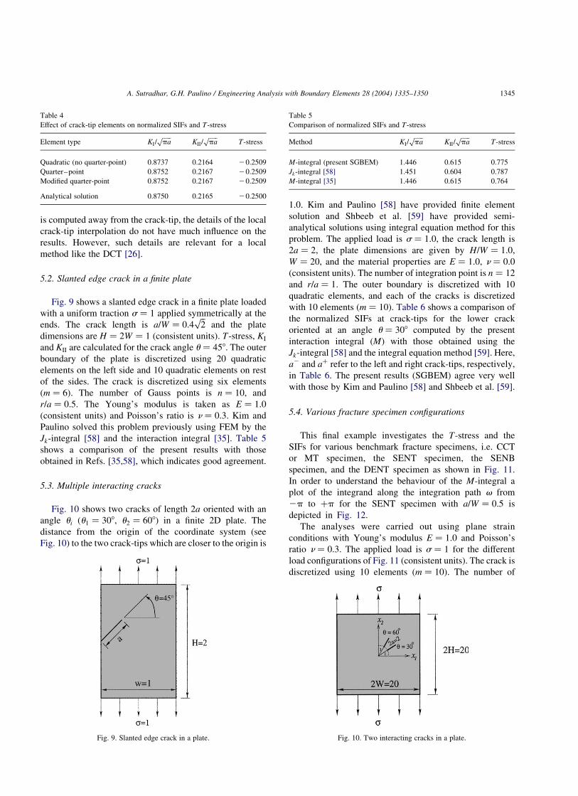
5.2. Slanted edge crack in a finite plate

Fig. 9 shows a slanted edge crack in a finite plate loaded

with a uniform traction s ¼ 1 applied symmetrically at the

ends. The crack length is a=W ¼ 0:4ffiffi2

pand the plate

dimensions are H ¼ 2W ¼ 1 (consistent units). T-stress, KI

and KII are calculated for the crack angle u ¼ 458: The outer

boundary of the plate is discretized using 20 quadratic

elements on the left side and 10 quadratic elements on rest

of the sides. The crack is discretized using six elements

ðm ¼ 6Þ: The number of Gauss points is n ¼ 10; and

r=a ¼ 0:5: The Young’s modulus is taken as E ¼ 1:0

(consistent units) and Poisson’s ratio is n ¼ 0:3: Kim and

Paulino solved this problem previously using FEM by the

Jk-integral [58] and the interaction integral [35]. Table 5

shows a comparison of the present results with those

obtained in Refs. [35,58], which indicates good agreement.

5.3. Multiple interacting cracks

Fig. 10 shows two cracks of length 2a oriented with an

angle ui (u1 ¼ 308; u2 ¼ 608) in a finite 2D plate. The

distance from the origin of the coordinate system (see

Fig. 10) to the two crack-tips which are closer to the origin is

1.0. Kim and Paulino [58] have provided finite element

solution and Shbeeb et al. [59] have provided semi-

analytical solutions using integral equation method for this

problem. The applied load is s ¼ 1:0; the crack length is

2a ¼ 2; the plate dimensions are given by H=W ¼ 1:0;

W ¼ 20; and the material properties are E ¼ 1:0; n ¼ 0:0

(consistent units). The number of integration point is n ¼ 12

and r=a ¼ 1: The outer boundary is discretized with 10

quadratic elements, and each of the cracks is discretized

with 10 elements ðm ¼ 10Þ: Table 6 shows a comparison of

the normalized SIFs at crack-tips for the lower crack

oriented at an angle u ¼ 308 computed by the present

interaction integral ðMÞ with those obtained using the

Jk-integral [58] and the integral equation method [59]. Here,

a2 and aþ refer to the left and right crack-tips, respectively,

in Table 6. The present results (SGBEM) agree very well

with those by Kim and Paulino [58] and Shbeeb et al. [59].

5.4. Various fracture specimen configurations

This final example investigates the T-stress and the

SIFs for various benchmark fracture specimens, i.e. CCT

or MT specimen, the SENT specimen, the SENB

specimen, and the DENT specimen as shown in Fig. 11.

In order to understand the behaviour of the M-integral a

plot of the integrand along the integration path v from

2p to þp for the SENT specimen with a=W ¼ 0:5 is

depicted in Fig. 12.

The analyses were carried out using plane strain

conditions with Young’s modulus E ¼ 1:0 and Poisson’s

ratio n ¼ 0:3: The applied load is s ¼ 1 for the different

load configurations of Fig. 11 (consistent units). The crack is

discretized using 10 elements ðm ¼ 10Þ: The number of

Table 4

Effect of crack-tip elements on normalized SIFs and T-stress

Element type KI=ffiffiffiffipa

pKII=

ffiffiffiffipa

pT-stress

Quadratic (no quarter-point) 0.8737 0.2164 20.2509

Quarter–point 0.8752 0.2167 20.2509

Modified quarter-point 0.8752 0.2167 20.2509

Analytical solution 0.8750 0.2165 20.2500

Fig. 9. Slanted edge crack in a plate.

Table 5

Comparison of normalized SIFs and T-stress

Method KI=ffiffiffiffipa

pKII=

ffiffiffiffipa

pT-stress

M-integral (present SGBEM) 1.446 0.615 0.775

Jk-integral [58] 1.451 0.604 0.787

M-integral [35] 1.446 0.615 0.764

Fig. 10. Two interacting cracks in a plate.


Gauss integration point is n ¼ 10: The outer boundary of

the CCT specimen is discretized with 10 quadratic elements

on each side, while for the rest of the specimens (SENT,

SENB and DENT), the outer boundary is discretized with 50

quadratic elements on the left edge and 30 quadratic

elements on the rest of the edges. Only half of the DENT

specimen was analysed due to its symmetry. Table 7 shows

good agreement between present results (SGBEM) and

those available in the literature. Fig. 13 shows the variation

of biaxiality ratio ðB ¼ Tffiffiffiffipa

p=KIÞ versus the ratio of crack

length to width a=W for various specimens ðH=W ¼ 12Þ and

compares with the results published by Fett et al. [60] using

the boundary collocation method, and by Kim and Paulino

[36] using the FEM. Notice that, for the SENB the present

solution (SGBEM) is closer to that by Fett et al. [60], while,

for the DENT, the present solution (SGBEM) is closer to

that by Kim and Paulino [36]. In general, all the solutions

(SGBEM, Fett et al. [60], and Kim and Paulino [36]) show

very good agreement in Fig. 13. The sign of the biaxiality

ratio changes from negative to positive as a=W increases in

SENT and SENB, while the sign remains the same for CCT

and DENT specimens.

6. Concluding remarks and extensions

The interaction integral method applied to mixed-mode

crack problems to evaluate T-stress and the SIFs using the

SGBEM has been presented. This method provides an

accurate and robust scheme for calculating the fracture

parameters. The numerical results obtained are in remark-

able agreement with known results for single and multiple

cracks. In general, the T-stress computations are more

demanding than those for SIFs (see Figs. 7 and 8). This

observation is in agreement with analogous studies in the

FEM field—see for example Refs. [36,61].

The influence of several parameters on the SIFs and

T-stress has been investigated, including the radius of the

integration contour ðrÞ; the number of integration points ðnÞ;

number of elements on the crack surface ðmÞ; and type of

crack-tip elements. Based on the experience acquired with

the present study, the number of Gauss points n $ 12 and

number of crack elements m $ 10 give accurate results for

all the problems investigated. A value of r=a . 0:3 is

sufficient for most problems, except when a=W is large,

where a is the length of the crack and W is the width of the

plate. A fracture criteria which includes the SIFs and T-stress

Table 6

Comparison of the normalized SIFs for the lower crack among various

methods

Method KIða2Þ=

ffiffiffiffipa

pKIIða

2Þ=ffiffiffiffipa

pKIða

þÞ=ffiffiffiffipa

pKIIða

þÞ=ffiffiffiffipa

p

M-integral

(present

SGBEM)

0.601 0.430 0.808 0.433

Jk-integral [58] 0.603 0.431 0.801 0.431

Integral

equation [59]

0.59 0.43 0.78 0.42

Fig. 11. Various fracture specimen configurations. The thickness of each

specimen is t:

Fig. 12. Variation of integrand of the M-integral along the integration path

v with r=a ¼ 0:5 where a is the crack length. Parameters adopted: m ¼ 10;

n ¼ 10:


can be implemented in the present code and used to predict

crack initiation angle (see, for example, Ref. [35]).

A potential extension of this SGBEM work includes

development of the two-state integral post-processing

approach to 3D crack problems. Another possible extension

involves fracture mechanics of non-homogeneous

materials, such as FGMs, which can make use of the new

Green’s functions developed by Chan et al. [62] in 2D and

Table 7

Normalized T-stress, biaxiality ratio (B), and normalized mode I SIF for various fracture specimens

Fracture specimen Sources T=s B ¼ Tffiffiffiffipa

p=KI KI=ðs=

ffiffiffiffipa

pÞ

CCT or MT (a=W ¼ 0:3; H=W ¼ 1:0) SGBEM (present) 21.1554 21.0286 1.1232

Chen et al. [15] 21.1554 21.0286 1.1232

Fett [60] 21.1557 21.0279 2

Leevers and Radon [10] – 21.0255 –

Cardew et al. [11] – 21.026 –

SENT (a=W ¼ 0:3; H=W ¼ 12) SGBEM (present) 20.6105 20.3679 1.6597

Kim and Paulino [36] 20.6139 20.3700 1.6594

Chen et al. [15] 20.6103 20.3677 1.6598

Fett [60] 20.6141 20.3664 –

Sham [13] 20.6142 20.3707 1.6570

SENT (a=W ¼ 0:5; H=W ¼ 12) SGBEM (present) 20.4184 20.1481 2.8241

Kim and Paulino [36] 20.4309 20.1481 2.8237

Chen et al. [15] 20.4217 20.1493 2.8246

Fett [60] 20.4182 20.1481 –

Sham [13] 20.4314 20.1529 2.8210

SENB (a=W ¼ 0:3; H=W ¼ 12) SGBEM (present) 20.0800 20.0712 1.1235

Chen et al. [15] 20.0792 20.0704 1.1241

Fett [60] 20.0771 20.0671 –

Sham [13] 20.0824 20.0734 1.1220

SENB (a=W ¼ 0:5; H=W ¼ 12) SGBEM (present) 0.3986 0.2662 1.4973

Chen et al. [15] 0.3975 0.2655 1.4972

Fett [60] 0.3921 0.2620 –

Sham [13] 0.3911 0.2616 1.4951

DENT (a=W ¼ 0:3; H=W ¼ 12) SGBEM (present) 20.5326 20.4780 1.1143

Kim and Paulino [36] 20.5384 20.4444 1.2115

Fett [60] 20.5319 20.4720 –

DENT (a=W ¼ 0:5; H=W ¼ 12) SGBEM (present) 20.5521 20.4725 1.1685

Kim and Paulino [36] 20.5597 20.4454 1.2567

Fett [60] 20.5216 20.4396 –

Fig. 13. Biaxiality ratio versus a=W for various fracture specimens.


Martin et al. [63] in 3D. Such Green’s function approach

allow the boundary element solution of fracture problems in

FGMs using a boundary-only approach (i.e. no domain

discretization).

Acknowledgements

We acknowledge the support from the Computational

Science and Engineering (CSE) Program (Prof. Michael

Heath, Director) at the University of Illinois at Urbana-

Champaign (UIUC) for the CSE Fellowship award to

A. Sutradhar. We thank Dr L.J. Gray, Oak Ridge National

Laboratory and Prof. Anh-Vu Phan, South Alabama

University, for helping us with the 2D SGBEM elasticity

code. We also thank Dr J.-H. Kim for providing the SIF

results for the slanted edge crack problem obtained by the

M-integral method using the FEM and also for useful

suggestions. G.H. Paulino acknowledges the support from

the National Science Foundation under grant CMS-0115954

(Mechanics and Materials Program).

Appendix A. Auxiliary fields for SIFs

The angular functions fijðuÞ in Eqs. (2) and (24) are

given by

f I11ðuÞ ¼ cos

u

21 2 sin

u

2sin

3u

2

� �;

f II11ðuÞ ¼ 2sin

u

22 þ cos

u

2cos

3u

2

� �;

f I22ðuÞ ¼ cos

u

21 þ sin

u

2sin

3u

2

� �;

f II22ðuÞ ¼ sin

u

2cos

u

2cos

3u

2;

f I12ðuÞ ¼ sin

u

2cos

u

2cos

3u

2;

f II12ðuÞ ¼ cos

u

21 2 sin

u

2sin

3u

2

� �

ðA1Þ

and giðuÞ in Eq. (25) is given by

gI1ðuÞ ¼

1

4ð2k2 1Þcos

u

22 cos

3u

2

� �;

gII1 ðuÞ ¼

1

4ð2kþ 3Þsin

u

2þ sin

3u

2

� �;

gI2ðuÞ ¼

1

4ð2kþ 1Þsin

u

22 sin

3u

2

� �;

gII2 ðuÞ ¼ 2

1

4ð2k2 3Þcos

u

2þ cos

3u

2

� �:

ðA2Þ

Appendix B. Displacement derivatives of auxiliary fields

for determining the T-stress

uaux1;1 ¼

2f cos u

pE0r1 2

sin2u

1 2 n

!

uaux2;1 ¼

þf sin u

pE0r1 2

cos2u

1 2 n

!

uaux1;2 ¼

2f sin u

pE0r1 þ

cos2u

1 2 n

!

uaux2;2 ¼

2f cos u

pE0r1 2

cos2u

1 2 n

!

ðB1Þ

where E0 is given by Eq. (23).

Appendix C. Displacement derivatives of auxiliary fields

for SIFs

uaux1;1 ¼

1

8mffiffiffiffiffi2pr

p KauxI ð2k2 3Þcos

u

2þ cos

5u

2

� ��

2KauxII ð2kþ 1Þsin

u

2þ sin

5u

2

� ��

uaux2;1 ¼

1


p KauxI 2ð2kþ 3Þsin

u

2þ sin

5u

2

� ��

2KauxII ð2k2 1Þcos

u

22 cos

5u

2

� ��

uaux1;2 ¼

1


p KauxI ð2kþ 1Þsin

u

2þ sin

5u

2

� ��

þKauxII ð2kþ 5Þcos

u

2þ cos

5u

2

� ��

uaux2;2 ¼

1


p KauxI ð2k2 1Þcos

u

22 cos

5u

2

� ��

þKauxII 2ð2k2 5Þsin

u

2þ sin

5u

2

� ��

ðC1Þ

Appendix D. Integration of the singular terms

in M-integral for calculating the T-stress

The contribution of the singular terms in the M-integral

for calculating the T-stress is evaluated. Let

M ¼ðG

{ðsik1auxik n1 2 ðsiju

auxi;1 þ saux

ij ui;1Þnj}dG: ðD1Þ

By selecting a circular integration path, the coefficients of

the singular terms Oðr21=2Þ from the integration over u from

2p to þp in Eq. (D1) are evaluated. After integration, the

first, second and the third term of Eq. (D1) yield

ðp

2psik1

auxik n1 du ¼ 2

1

210

fffiffi2

pKIð49k2 27Þ

pffiffiffiffirp

pm

; ðD2Þ


2ðp

2psiju

auxi;1 nj du ¼ 2

1

105

fffiffi2

pKIð7kþ 3Þ

pffiffiffiffirp

pm

; ðD3Þ

and

2ðp

2psaux

ij ui;1nj du ¼ 21

10

fffiffi2

pKIð3k2 1Þ

pffiffiffiffirp

pm

; ðD4Þ

respectively. These three terms add to zero.

References

[1] Rice JR. Path-independent integral and the approximate analysis of

strain concentration by notches and cracks. J Appl Mech Trans ASME

1968;35(2):379–86.

[2] Anderson TL. Fracture mechanics: fundamentals and applications.

Boca Raton, FL: CRC Press LLC; 1995.

[3] Williams JG, Ewing PD. Fracture under complex stress—the angled

crack problem. Int J Fract 1972;8(4):416–41.

[4] Ueda Y, Ikeda K, Yao T, Aoki M. Characteristics of brittle failure

under general combined modes including those under bi-axial tensile

loads. Eng Fract Mech 1983;18(6):1131–58.

[5] Smith DJ, Ayatollahi MR, Pavier MJ. The role of T-stress in brittle

fracture for linear elastic materials under mixed-mode loading.

Fatigue Fract Eng Mater Struct 2001;24(2):137–50.

[6] Cotterell B, Rice JR. Slightly curved or kinked cracks. Int J Fract

1980;16(2):155–69.

[7] Du Z-Z, Hancock JW. The effect of non-singular stresses on crack-tip

constraint. J Mech Phys Solids 1991;39(3):555–67.

[8] O’Dowd NP, Shih CF, Dodds JrRH. The role of geometry and crack

growth on constraint and implications for ductile/brittle fracture. In:

Constraint effects in fracture theory and applications. volume 2 of

ASTM STP 1244, American Society for Testing and Materials; 1995.

p. 134–59.

[9] Larsson SG, Carlson AJ. Influence of non-singular stress terms and

specimen geometry on small-scale yielding at crack tips in elastic–

plastic materials. J Mech Phys Solids 1973;21(4):263–77.

[10] Leevers PS, Radon JCD. Inherent stress biaxiality in various fracture

specimen. Int J Fract 1982;19(4):311–25.

[11] Cardew GE, Goldthorpe MR, Howard IC, Kfouri AP. On the elastic

T-term. Fundamentals of deformation and fracture: Eshelby memorial

symposium. 1985.

[12] Kfouri AP. Some evaluations of the elastic T-term using Eshelby’s

method. Int J Fract 1986;30(4):301–15.

[13] Sham TL. The determination of the elastic T-term using higher-order

weight functions. Int J Fract 1991;48(2):81–102.

[14] Wang Y-Y, Parks DM. Evaluation of the elastic T-stress in surface-

cracked plates using the line-spring method. Int J Fract 1992;56(1):

25–40.

[15] Chen CS, Krause R, Pettit RG, Banks-Sills L, Ingraffea AR.

Numerical assessment of T-stress computation using a p-version

finite element method. Int J Fract 2001;107(2):177–99.

[16] Sladek J, Sladek V, Fedelinski P. Contour integrals for mixed-mode

crack analysis: effect of nonsingular terms. Theor Appl Fract Mech

1997;27(2):115–27.

[17] Nakamura T, Parks DM. Determination of T-stress along three-

dimensional crack fronts using an interaction integral method. Int J

Solids Struct 1992;29(13):1597–611.

[18] Liu GR. Mesh free methods: moving beyond the finite element

method. Boca Raton, FL: CRC Press LLC; 2003.

[19] Bonnet M, Maier G, Polizzotto C. Symmetric Galerkin boundary

element method. Appl Mech Rev 1998;51(11):669–704.

[20] Bonnet M. Exploiting partial or complete geometrical symmetry in

3D symmetric Galerkin indirect BEM formulations. Int J Numer Meth

Eng 2003;57(8):1053–83.

[21] Gray LJ, Griffith B. A faster Galerkin boundary integral algorithm.

Commun Numer Meth Eng 1998;14(12):1109–17.

[22] Sirtori S. General stress analysis method by means of integral

equations and boundary elements. Meccanica 1979;14:210–8.

[23] Hartmann F, Katz C, Protopsaltis B. Boundary elements and

symmetry. Ingenieur Archiv 1985;55(6):440–9.

[24] Sirtori S, Maier G, Novati G, Miccoli S. A Galerkin symmetric

boundary element method in elasticity: formulation and implemen-

tation. Int J Numer Meth Eng 1992;35(2):255–82.

[25] Gray LJ, Paulino GH. Symmetric Galerkin boundary integral fracture

analysis for plane orthotropic elasticity. Comput Mech 1997;20(1–2):

26–33.

[26] Gray LJ, Phan A-V, Paulino GH, Kaplan T. Improved quarter-point

crack tip element. Eng Fract Mech 2003;70(2):269–83.

[27] Chen FHK, Shield RT. Conservation laws in elasticity of the J-integral

type. J Appl Math Phys (ZAMP) 1977;28:1–22.

[28] Yau JF, Wang SS, Corten HT. A mixed-mode crack analysis of

isotropic solids using conservation laws of elasticity. J Appl Mech

Trans ASME 1980;47(2):335–41.

[29] Wang SS, Corten HT, Yau JF. Mixed-mode crack analysis of

rectilinear anisotropic solids using conservation laws of elasticity. Int

J Fract 1980;16(3):247–59.

[30] Gosz M, Moran B. An interaction energy integral method for

computation of mixed-mode stress intensity factors along non-planar

crack fronts in three dimensions. Eng Fract Mech 2002;69(3):

299–319.

[31] Dolbow J, Gosz M. On the computation of mixed-mode stress

intensity factors in functionally graded materials. Int J Solids Struct

2002;39(9):2557–74.

[32] Rao BN, Rahman S. Mesh-free analysis of cracks in isotropic

functionally graded materials. Eng Fract Mech 2003;70(1):1–27.

[33] Kim J-H, Paulino GH. An accurate scheme for mixed-mode fracture

analysis of functionally graded materials using the interaction integral

and micromechanics models. Int J Numer Meth Eng 2003;58(10):

1457–97.

[34] Kim J-H, Paulino GH. The interaction integral for fracture of

orthotropic functionally graded materials: evaluation of stress

intensity factors. Int J Solids Struct 2003;40(15):3967–4001.

[35] Kim J-H, Paulino GH. T-stress, mixed-mode stress intensity factors,

and crack initiation angles in functionally graded materials: a unified

approach using the interaction integral method. Comput Meth Appl

Mech Eng 2003;192(11):1463–94.

[36] Paulino GH, Kim J-H. A new approach to compute T-stress in

functionally graded materials by means of the interaction integral

method. Eng Fract Mech 2004;71(13–14):1907–50.

[37] Kim J-H, Paulino GH. T-stress in orthrotropic functionally graded

materials: Lekhnitskii and Stroh formalisms. Int J Fract 2004; [in

press].

[38] Banerjee PK. The boundary element methods in engineering. London:

McGraw-Hill; 1994.

[39] Aliabadi MH. Evaluation of mixed mode stress intensity factors using

the path independent integral. In: Proceedings of 12th International

Conference on Boundary Element Methods, Southampton. Compu-

tational Mechanics Publications; 1990. p. 281–92.

[40] Sladek J, Sladek V. Evaluation of T-stresses and stress intensity

factors in stationary thermoelasticity by the conservation integral

method. Int J Fract 1997;86(3):199–219.

[41] Denda M. Mixed mode I, II and III analysis of multiple cracks in plane

anisotropic solids by the BEM: a dislocation and point force approach.

Eng Anal Bound Elem 2001;25(4–5):267–78.

[42] Wen PH, Aliabadi MH. A contour integral for the evaluation of stress

intensity factors. Appl Math Model 1995;19(8):450–5.

[43] Aliabadi MH. Boundary element formulations in fracture mechanics.

Appl Mech Rev 1997;50(2):83–96.

[44] Aliabadi MH. The boundary element method: vol 2. Application in

solids and structures. England: Wiley; 2002.


[45] Williams ML. On the stress distribution at the base of a stationary

crack. J Appl Mech Trans ASME 1957;24(1):109–14.

[46] Michell JH. Elementary distributions of plane stress. Proc Lond Math

Soc 1900;32:35–61.

[47] Timoshenko SP, Goodier JN. Theory of elasticity, 3rd ed. New York:

McGraw-Hill; 1987.

[48] Hills DA, Kelly PA, Dai CN, Korsunsky AM. Solution of crack

problems: the distributed dislocation technique. The Netherlands:

Kluwer Academic Publishers; 1996.

[49] Rizzo FJ. An integral equation approach to boundary value problems

of classical elastostatics. Q Appl Math 1967;25:83–95.

[50] Crouch SL. Solution of plane elasticity problems by the displacement

discontinuity method. Int J Numer Meth Eng 1976;10:301–43.

[51] Crouch SL, Starfield AM. Boundary element methods in solid

mechanics. London: George Allen and Unwin; 1983.

[52] Phan A-V, Napier JAL, Gray LJ, Kaplan T. Symmetric-Galerkin

BEM simulation of fracture with frictional contact. Int J Numer Meth

Eng 2003;57(6):835–51.

[53] Holzer SM. The symmetric Galerkin BEM for plane elasticity: scope

and applications. In: Hirsch C, editor. Numerical methods in

engineering ’92. Amsterdam: Elsevier; 1992.

[54] Li S, Mear ME, Xiao L. Symmetric weak form integral equation

method for three-dimensional fracture analysis. Comput Meth Appl

Mech Eng 1998;151(3–4):435–59.

[55] Henshell RD, Shaw KG. Crack tip finite elements are unnecessary. Int

J Numer Meth Eng 1975;9:495–507.

[56] Barsoum RS. On the use of isoparametric finite elements in linear

fracture mechanics. Int J Numer Meth Eng 1976;10:25–37.

[57] Gray LJ, Paulino GH. Crack tip interpolation, revisited. SIAM J Appl

Math 1998;58(2):428–55.

[58] Kim J-H, Paulino GH. Finite element evaluation of mixed-mode stress

intensity factors in functionally graded materials. Int J Numer Meth

Eng 2002;53(8):1903–35.

[59] Shbeeb NI, Binienda WK, Kreider KL. Analysis of the driving

forces for multiple cracks in an infinite nonhomogeneous plate. Part

II. Numerical solutions. J Appl Mech Trans ASME 1999;66(2):

501–6.

[60] Fett T. T-stresses in rectangular plates and circular disks. Eng Fract

Mech 1998;60(5–6):631–52.

[61] ABAQUS/standard user’s manual. Version 6.3, vol. I. Pawtucket, RI,

USA: Hibbitt, Karlsson and Sorensen Inc.; 2003.

[62] Chan Y-S, Gray LJ, Kaplan T, Paulino GH. Green’s function for a

two-dimensional exponentially-graded elastic medium. Proceedings

of the Royal Society of London Series A: Mathematical, Physical and

Engineering Sciences. 2004. [in press].

[63] Martin PA, Richardson JD, Gray LJ, Berger J. On Green’s function for

a three-dimensional exponentially-graded elastic solid. Proc R Soc

Lond Ser A: Math Phys Eng Sci 2002;458(2024):1931–47.


Documents

Symmetric Galerkin boundary element computation … · Symmetric Galerkin boundary element computation of T-stress ... constraint and fracture toughness ... approach involves one