The Signaling Value of a High School Diploma

Paco Martorell

RAND

Damon Clark

University of Florida, NBER, IZA

12 August 2010

Abstract

Although economists acknowledge that various indicators of educational attainment (e.g., highest

grade completed, credentials earned) might serve as signals of a worker’s productivity, the practical

importance of education-based signaling is not clear. In this paper we estimate the signaling value

of a high school diploma, the most commonly held credential in the U.S. To do so, we compare the

earnings of workers that barely passed and barely failed high school exit exams, standardized tests

that, in some states, students must pass to earn a high school diploma. Since these groups should, on

average, look the same to firms (the only difference being that "barely passers" have a diploma while

"barely failers" do not), this earnings comparison should identify the signaling value of the diploma.

Using linked administrative data on earnings and education from two states that use high school exit

exams (Florida and Texas), we estimate that a diploma has little effect on earnings. For both states, we

can reject that individuals with a diploma earn eight percent more than otherwise-identical individuals

without one; combining the state-specific estimates, we can reject signaling values larger than five or six

percent. While these confidence intervals include economically important signaling values, they exclude

both the raw earnings difference between workers with and without a diploma and the regression-adjusted

estimates reported in the previous literature.

∗For useful discussions, we thank Kelly Bedard, Ken Chay, Mike Geruso, Marco Manacorda, Rob McMillan, Devah Pager,Craig Riddell and, especially, David Lee. For helpful comments and suggestions, we thank seminar participants at Bristol

University, Brown University, Columbia University, the Florida Department of Education, Harvard University, London School

of Economics, Northwestern University, Pompeu Fabra, Princeton University, RAND, Rutgers University, University of Toronto,

UC Davis, UC Irvine, UC Santa Barbara, University of Florida, the SOLE 2010 conference, the NBER 2010 Summer Institute

and the Southern California Conference of Applied Microeconomics (Claremont McKenna College). Clark thanks the Florida

Department of Education for generously supplying the Florida data used in this paper and for providing invaluable information

on the relevant institutions. Much of this work was completed while Clark was visiting the Industrial Relations Section at

Princeton University. We thank Marion Aouad and Yu Xue for excellent research assistance. Financial support was generously

provided by the U.S. Department of Education (under grant R305R060096). The opinions expressed in this paper are ours, and

do not necessarily reflect the views of the Florida Department of Education, the Texas Department of Education or the U.S.

Department of Education.

1 Introduction

The concept of market signaling, most closely associated with Spence (1973), has added greatly to our

understanding of markets characterized by incomplete information. In a labor market context, it implies

that firms with incomplete information about worker productivity may base productivity expectations, and

thus wages, on unalterable "indices" such as race and sex, and alterable "signals" such as educational

attainment. In principle, various types of educational outcomes could act as signals of ability, including

highest grade completed, school performance (e.g., grades), school attended (e.g., a selective college) and

receipt of an educational credential such as a high school diploma or college degree.

For two reasons, tests of education-based signaling have often focused on the signaling content of edu-

cational credentials.1 First, it has long been thought that credential receipt may send a particularly strong

signal. As Layard and Pschacharopoulos (1974) observed, “graduation from a course should provide more

evidence of ability and staying power than mere attendance for a number of years” (p.989). Second, because

credentials are, ultimately, pieces of paper, they cannot have a direct effect on productivity. In principle

then, one could estimate the signaling value of a credential by randomly assigning credentials among equally

productive workers and estimating the wage return to holding the credential.2 Since workers in these "treat-

ment" and "control" groups would appear equally productive to firms (at least on average), the wage return

would capture the signaling value of the credential.

In this paper we focus on the signaling value of a high school diploma. Since this is the most commonly

held credential in the US, it should be relatively well understood, and might act as an especially strong

signal of productivity.3 The existing evidence supports this conjecture. In particular, estimates of the return

to a high school diploma in regressions of wages on diploma receipt and other controls suggests that a

diploma increases wages by between ten and twenty percent (e.g.,Park (1994), Jaeger and Page (1996)).4

These regression-based estimates do, however, rest on the assumption that these controls capture all of the

market’s other productivity information. If the market has productivity information not captured by these

1Other approaches test whether the private returns to education exceed the social returns to education (as they would if

signaling dominated any positive externalities associated with education - Acemoglu and Angrist (2000)); whether education

policy changes impact the educational decisions of students they do not directly affect (as they would if those students wished to

differentiate themselves from the directly-affected students - Lang and Kropp (1986) and Bedard (2001)); whether wage equations

fit better for workers in occupations in which productivity cannot be observed (as they would if productivity expectations and

hence wages in those occupations were based on signals such as education - Riley (1979)) and whether there are lower returns

to education among the self-employed (as there would be if a component of the return among the non self-employed reflected

the signaling value of education - Wolpin (1977)).2 Such an experiment would have to be limited to a small subset of workers and would have to involve a well-known credential

(such as a high school diploma). If all credentials were randomly assigned, or if the credential was unfamiliar to firms, then by

design, the credential would not be a useful signal of productivity. The theoretical framework (below) makes precise the sense

in which credentials are quasi-randomly assigned in the settings that we study.3 http://www.census.gov/population/www/socdemo/education/cps2009.html4An earlier generation of studies addressed this question by assessing whether there was an especially large return to

completing twelve years of schooling. As Park (1994) concluded, "it appears that these types of estimates...are sensitive to

model specification" (p.5). For example, using this approach, he estimated diploma returns between three and thirteen percent.

Hungerford and Solon (1987) estimated diploma returns between three and eight percent.

1

controls (e.g., how a worker presents herself when applying for a job), and if this is correlated with diploma

receipt, the estimated diploma returns will overstate the signaling value of the diploma. Many of the papers

in this literature acknowledge these problems.5

More convincing estimates of the signaling value of a high school diploma might be obtained from research

designs that better approximate the random assignment of high school diplomas among workers. In a

seminal paper in the empirical signaling literature, Tyler, Murnane, and Willett (2000) employ a difference-

in-difference strategy that mimics this randomization to estimate the signaling value of a GED.6 Their key

insight is that across-state variation in the scores required to earn a GED generates across-state variation in

GED status among workers with similar GED scores (hence similar productivity). Using this strategy, they

estimate the signaling value of the GED to be between 12 percent and 20 percent for whites and zero for

blacks. While these estimates are consistent with the earlier sheepskin estimates (at least for whites), there

are two reasons why they may be an unreliable guide to the signaling value of a high school diploma. First,

subsequent papers in the GED literature, based on versions of the same strategy, find much smaller effects,

suggesting there is no consensus as to the signaling value of the GED.7 Second, as Jepsen, Mueser, and

Troske (2010) point out in a recent paper, much of this literature has drawn comparisons between workers

that pass GED exams and workers that fail GED exams and do not retake them. If retaking is selective

(e.g., if more motivated workers retake), this could bias this literature towards finding positive GED effects.8

This paper estimates the signaling value of a high school diploma by exploiting variation in high school

diploma receipt generated by high school exit exams, standardized tests that, in some states, students must

pass to earn a high school diploma. More specifically, we estimate the signaling value of a diploma via a

regression discontinuity strategy that compares the earnings of workers that narrowly passed these exams

(and earned a high school diploma) with the earnings of students that narrowly failed these exams (and

did not). The key assumption is that workers that narrowly passed and narrowly failed these exams will

have the same productive characteristics as observed by firms (at least on average), such that any earnings

discontinuity can be interpreted as the signaling value of the diploma. This argument is intuitive, but we

formalize it in the context of a simple theoretical framework. This framework clarifies the conditions under

which the signaling value of the diploma can be identified, the relation between these conditions and those

5Hungerford and Solon (1987) note that their regression analyses "may be biased by omission of ability variables or other

factors correlated with degree completion” (p.177). Jaeger and Page (1996) note that “we are reluctant to interpret our results

as purely causal effects of diploma receipt on wages” (p.739).6The General Educational Development (GED) degree is a credential that is typically pursued by high school dropouts. It

is intended to be equivalent to a high school diploma.7Using various strategies to compare the earnings of workers that passed and failed GED exams in the same state, Tyler

(2004b) finds signaling values of around 10%. Lofstrum and Tyler (2007) use difference-in-difference strategies based on within-

state variation in GED passing scores and cannot reject zero signaling values. Cameron and Heckman (1993) also argue that

there are small returns to a GED.8Jepsen, Mueser, and Troske (2010) find little return to the GED when instrumenting GED status with whether the GED

exams were passed at the first attempt, although these estimates are fairly imprecise.

2

required by the previous regression-based studies, and the likely determinants of the signaling value of the

diploma.

For two states that use high school exit exams (Florida and Texas), we were able to link detailed education

records to high-quality administrative earnings data. The individuals in these datasets attended high school

in the 1990s and 2000s, and we observe them in the labor market until they are approximately age 25. Using

these data, we estimate the signaling value of a high school diploma. We begin by reporting regression-based

estimates, all of which suggest large signaling values, between ten and twenty percent (i.e., in line with the

previous literature). We then report estimates based on our preferred discontinuity approach. These are

much smaller than the regression-based estimates and suggest that the diploma has little effect on earnings.

This conclusion holds when we split by sex and race and when we examine the experience profile of signaling

values. When we pool across years and combine estimates from the two states, we can reject signaling values

larger than six percent of mean earnings. This would still be an economically important effect, but it is much

smaller than raw earnings difference between workers with and without a diploma and the regression-adjusted

estimates reported in the previous literature.

Although we think that this discontinuity approach is highly credible, two caveats must be applied to our

estimates. First, to ensure that exam outcomes affect only diploma status (as opposed to length of schooling

or curriculum), we focus on students that take the exit exam at the end of twelfth-grade. Since students take

the exam for the first time in tenth grade, and can retake it several times between tenth grade and the end

of twelfth grade, this means that we focus on a relatively small group of academically marginal students that

have already failed the exam at least once, and often several times. If signaling values are heterogeneous

(e.g., because they vary with the other information held by firms or with the type of jobs performed by

workers), this means that our estimates will be specific to these academically marginal students. In defense

of our approach, we note that if policies target academic performance/standards but also affect high school

graduation rates, it is exactly these academically marginal students whose graduation status will likely be

affected by these policies. As such, our estimates can tell us whether the returns to these policies can be

attributed to the signaling value of a high school diploma. Moreover, we show that a high school diploma is

a good predictor of earnings for these types of students - almost as good a predictor of their earnings as it

is of the earnings of academically stronger groups. Since this suggests that a diploma could, potentially, be

used to infer something about the productivity of these workers, it is not obvious why the signaling value

of the diploma should be especially low for them. The second caveat is that diploma receipt may affect

downstream outcomes for these students (e.g., whether to attend college). While this would complicate the

interpretation of our estimates, we show that diploma receipt has relatively small impacts on a variety of

post-secondary education outcomes, and we argue that these are unlikely to account for any of our results.

3

We suspect that our discontinuity-based estimates are smaller than the raw earnings differences and the

regression-based estimates because the diploma has less predictive power for earnings conditional on the

other information observed by firms (and implicitly controlled for by our strategy). Some of this information

will be acquired at the time of hiring (e.g., from employment histories, interviews and performance tests)

and firms may learn quickly about productivity thereafter (Farber and Gibbons (1996), Altonji and Pierret

(2001) and Lange (2007)). The information content of the diploma will be further weakened by the potential

for diploma misreporting, a likely result of the difficulty of verifying diploma receipt (Bishop (1988)). Since

similar considerations likely apply to other lower-level indicators of educational attainment, (e.g., grade

dropped out of high school), our findings suggest that among workers without a college degree, the signaling

value of various indicators of educational attainment is likely much smaller than was previously thought.

2 Theoretical Framework

We begin the paper by laying out a simple theoretical framework. This helps to clarify the assumptions

under which we identify the signaling value of a credential and it connects these assumptions to those on

which estimates in the previous literature were based. It also helps in interpreting the signaling values that

we estimate. For example, it shows why these signaling values might differ across workers (i.e., heterogeneous

effects).

2.1 Basic Setup

We assume that individuals live for two periods. In the first period they attend school and in the second

period they work. We characterize individuals in terms of a one-dimensional index of ability as represented

by the continuous random variable . We assume that ability is known to individuals at the start of the first

period but is never observed by firms.

In our setup, students earn a credential when a one-dimensional measure of school performance exceeds

some threshold level . That is, = 1 iff ≥ .9 We assume that is determined by = b + , where

b = 0+1. The variable is the amount of study effort exerted in the schooling period. We think of study

effort as encompassing various behaviors and activities that improve school performance (given ability).10

We assume that study effort ( ) is costly for all individuals ( 0) and that costs are decreasing (or

at least non-increasing) in ability ( ≤ 0). The variable is a mean-zero random variable assumed to be

9The one-dimensional nature of is unrestrictive. In the absence of exit exams, could refer to the minimum number of

credits needed to graduate; in the presence of exit exams, could refer to the score on the exit exam as well as other graduation

requirements.10 In the absence of exit exams, studying could correspond to attendance; in the presence of exit exams, it could correspond

to exam preparation.

4

independent of b and continuously distributed on the real line. This assumption captures the fact that thereis some uncertainty determining school performance (i.e., students do not exercise complete control over )

and that all students will obtain a credential with probability between zero and one.11

We assume that second-period productivity (denoted ) is given by = + 2, a function of ability

and first-period study effort. This captures the idea that productivity is related to underlying ability and

also implies that studying might be valued by firms (if 2 0). We assume that firms do not observe .

Instead, they observe , whether a worker has a diploma, and , a noisy signal of productivity. We assume

= + , where is a mean-zero random variable assumed to be independent of . We will describe

as a worker’s type, as observed by a firm. This could be based, for example, on performance at a job

interview. On average, more productive workers will perform better at job interviews, but there is some

slippage between productivity and interview performance. We assume individuals are perfect substitutes

in production and assume there are a large number of risk-neutral firms competing for their services. This

implies that the second-period wage equals expected productivity. Since productivity expectations will be

based on a worker’s type () and whether she holds a credential (), this implies that wages can be written:

= () (1)

2.2 Signaling Equilbria and Signaling Values

These assumptions describe a game of incomplete information in which firms choose wage functions ( = 1

) and ( = 0 ) and workers choose study level (). A perfect Bayesian equilibrium of this game

must satisfy two properties. First, given the wage functions, given knowledge of the distribution of and

and assuming rational expectations, the study choices () must maximize the expected utility of workers.

Second, given these study choices, given knowledge of the distribution of and and assuming rational

expectations, these wage functions must ensure that firms make zero profits.

We can define the signaling value of a credential for a worker of type as:

() = ( = 1 )− ( = 0 )

This is the wage difference between workers with and without a credential, conditional on the other produc-

tivity information observed by firms.

11There are two other ways to introduce uncertainty into this process. First, students may be imperfectly informed about

ability . Then, even if high school performance is a deterministic function of ability and study effort, students will not be able

to forecast performance precisely. Second, students might not know how productive will be their study effort (i.e., 1 could be

a random variable whose distribution varied across students). These will have similar implications to the case considered in the

text.

5

Example of a Signaling Equilibrium

It is worth considering the signaling equilibrium in a simple special case of this framework. Suppose that

(1) ability is uniformly distributed on [ ] where =0(i.e., all students must exert some study effort

to obtain the credential), (2) study costs are () = , where 2+120

(i.e., sufficiently high so that not

all students will obtain the credential), (3) = 0, so that there is no uncertainty in the credential acquisition

process and (4) the firm observes only , so that wages will be conditioned on only. This implies that

a signaling equilibrium must feature an ability cutoff below which workers exert zero effort (and do not get

a credential) and above which workers exert just enough study effort to get the credential. It is simple to

show that there is only one such equilibrium, which can be characterized by:

∗ = [ − ][

2(− 2)]

() =

⎧⎪⎨⎪⎩ 0 if ∗

01( − ) if ≥ ∗

⎫⎪⎬⎪⎭ − ∗

− =

120

[1

(− 2)] 1

The signaling value is not a function of because we assumed that firms observe only .12 We return to

this equilibrium below.

2.3 Two Approaches to Identification

There are two possible approaches to identifying (). First, the researcher could assume that observable

covariates serve as adequate proxy for . Then he could estimate type-specific signaling values by comparing

wages by credential status for workers of the same type. This is the basis of the regression-based approaches

used in the previous literature. The obvious limitation with these regression-based approaches is that the

covariates may not fully control for . If, as expected, is positively correlated with , and hence ,

estimates of the signaling value of the credential will be biased upwards.

Some (e.g., Riley (2001)) have also criticized these regression-based approaches for not explaining what

drives variation in credential status among workers who appear similar to firms (i.e., what drives variation

in conditional on ). This framework shows that this variation can be driven by either or . Variation

driven by implies that workers with the same ability , the same school performance , the same produc-

12An equilibrium is a value of such that, given the optimal effort strategies, [| = 1] − [| = 0] = . For a given

, the cutoff ability level ∗ solves [ 01( −∗)] = . For a given ∗, [| = 1]−[| = 0] =

−2

+021

( −∗).

Equating and using () = gives−∗− , which can be used to derive . There is only one solution to the equation

[| = 1]−[| = 0] = . Given the assumption on , this satisfies 0 −∗− 1.

6

tivity and the same productivity signal can differ in diploma status by virtue of getting a good or bad

draw of (i.e., being lucky in school). Variation driven by implies that workers that have different levels

of ability , different levels of school performance , different values of diploma status and different levels

of productivity can have the same productivity signal by virtue of getting a good or bad draw of (i.e.,

being lucky in the interview).

This discussion suggests a second, discontinuity-based approach that exploits variation in and rests

on weaker assumptions than those required by the regression-based approach. Specifically, we can compare

workers whose school performance was just good enough to earn the credential with those whose performance

falls just below the cutoff :

( ) = [ | = ]− lim∆→0+

[ | = −∆]

The key assumption underpinning this approach is that (| = ) is smooth through = , that is, if

the distribution of ability is the same for workers in a small interval around . If this condition holds,

then it follows that ( ) =R

()(| = ) 13 In other words, this discontinuity-based approach

identifies a weighted average of type-specific signaling values (), where the weights are the probabilities

that workers are of different types conditional on school performance being close to .

In this context, (| = ) will be smooth through if school performance is uncertain (i.e., the

distribution of is non-degenerate).14 ,15 If, instead, students have complete control over school performance

(so that it exhibits no randomness), then a discontinuity-based approach would be impossible. That is

because the distribution of school performance will have zero density just to the left of the threshold. The

intuition is that when students have complete control over school performance, they will never choose a

study level that results in them narrowly failing to pass. The example equilibrium described above exhibited

this property. School performance was certain, workers with ability = ∗ exerted positive study effort and

13The continuity of (| = ) ensures the continuity of (| = ) because (| = ) =(|)(| = ) and

because (|) is not a function of . It then follows that: [ | = ] − lim∆→0+ [ | = − ∆] =

( =

1)(| = ) − lim∆→0

( = 0)(| = − ∆) =

[ ( = 1) − ( = 0)](| = ) =

()(| = ).14Because we have assumed that is a continuous random variable distributed on the real line, we have that for any equilibrium

study strategies and for every ability type 0 (|) = [ − ()] 1 . This implies that for all , ( − ())and ( − ()) are continuous at = and ( − ()) 0 when = . Since () =

( − ())(), this

implies that () is continuous at = . Since this implies that () and ( − ()) are continuous in , it implies that

(0| = ) =(|0)(0)

()=

(−\(0))(0)()

is continuous at = .15This is a special case of the conditions required for the validity of a regression discontinuity design. These were introduced

by Lee (2008) in a far more general setting than the linear additive model for considered here.

7

just passed while workers with ability ∗ exerted zero study effort and failed by 1(∗).16 It is easy to

show that this "zero density" result carries through to the more general case in which school performance is

certain and the firm also observes worker’s type (in that example firms observed only ).17

2.4 Interpretation

Because signaling values are conditioned on , they can differ across types of workers. To the extent that

specific subgroups are associated with specific types, this implies that they can also vary across subgroups

(e.g., sex and race). Average signaling values can also vary across credentials. To see this, return to the simple

example considered above and note that the equilibrium signaling value was increasing in 2, the productivity

returns to the studying required to obtain the credential. The dependence on 2 implies that the signaling

value will be higher the more strongly correlated are the credential requirements and productivity. This point

was made by Dee and Jacob (2006) in their discussion of the effects of expanding high school graduation

requirements to include high school exit exams.

Note finally that there are three cases in which signaling values are zero (i.e., the diploma carries no

information).18 First, if the firms observe (i.e., observe exit exam scores in our context), the wage will

be conditioned on and rather than and . Conditional on , there is no overlap in hence the

signaling value is no longer defined as it was above. Moreover, the difference in wages among workers on

either side of the passing threshold will be zero, since (| = ) = lim∆→0+ (| = − ∆) hence[ | = ]− lim∆→0+ [ | = −∆] = 0. Second, if firms have a lot of information, then the credentialbecomes redundant. In the extreme case where firms observe worker productivity (i.e., = 0), wages equal

observed productivity and () = () = () and ( = 1 ) − ( = 0 ) = 0. Third,

the signaling value will also be zero if misreporting of diploma receipt ensures that reported diploma receipt

is uncorrelated with true diploma receipt. We return to these possibilities when discussing our results below.

16Since workers with = ∗ studied just enough to meet the cutoff, we know that (∗) = 0∗+1(

∗) = . Since workers

with ability below ∗ did no studying, we know that their high school performance was lim∆→0+

(∗) = 0∗ = − 1(

∗),

hence 1(∗) below the cutoff.

17We want to show that we cannot have an equilibrium in which = 0 (i.e., no uncertainty), () is continuous at = =

(i.e., density on both sides of the threshold) and some () 0 (i.e., positive signaling values for some types). Notice first that

if () is continuous at = , then there exist some for which ≥ and some for which . Given our assumptions on

study costs and 0 1 2, must be increasing in among both groups. Further, () (∗) for all ∗ where (∗) = .

Since () is continuous at = , we must have lim→0+

(∗ −) = (∗) = (if lim→0+

(∗ −) , there would be a

"hole" in the distribution of just below ). Since = 1 + 2, this implies that we must have lim→0+

(∗ −) = (∗).

Since study costs are continuous in ability and study effort, then for study strategies to take this form, we must have that

lim→0+

[ |∗ − (∗ −) = 0] ≥ [ |∗ (∗) = 1]. If this was not the case, an individual with ability ∗

would do better by choosing (∗) such that = . But this implies that [ | = ]− lim∆→0+ [ | = −∆] ≤ 0,which cannot be the case if there exists a positive signaling value.18We assume there is a mechanism linking school performance and productivity. That is, we rule out the possibility that

= 0 and 0 = 2 = 0 (i.e., no mechanism linking and ), such that school performance does not predict productivity

(hence ( = 1 )− ( = 0 ) = 0). That is because, in our data, exit exam scores are strongly correlated with wages

(hence productivity).

8

2.5 Relation to the Literature

The framework outlined above is, we believe, a useful tool for analyzing the signaling value of a credential.

It does, however, differ from what might be considered the canonical model of education-based signaling.19

In this model, outlined for example by Borjas (2005) (pp. 260-265) and Ehrenberg and Smith (2009) (pp.

307-312), workers signal unobserved (to the firm) ability via their choice of how many years to spend in

school. Provided firms observe years of schooling, and provided the cost of schooling is decreasing in ability,

schooling can act as an ability signal even if it is completely unproductive.

There are two differences between this textbook framework and our credentials framework. First, in this

textbook framework, there is more education investment in a signaling equilibrium than there is in the full-

information (socially optimal) equilibrium. This is obvious when schooling is completely unproductive (i.e.,

the socially optimal level is zero); it also true in the more general case in which schooling is both productive

and, potentially, used as an ability signal.20 In contrast, it is unclear in our framework whether investments

in education (i.e., studying) are greater in a signaling equilibrium or the full-information equilibrium.21 ,22

Second, in the textbook framework it is impossible to identify the signaling value of education by comparing

the wages of workers with differing levels of schooling. Even randomization of years of schooling cannot

unbundle the productivity and signaling components unless the researcher knows the magnitude of the

productivity component. In contrast, because a credential has no productive component (i.e., it is a piece

of paper), quasi-randomization of a credential can identify its signaling value. This is the approach pursued

in this paper.

Despite these differences, the same conditions are required to sustain signaling in both frameworks. In

particular, in both frameworks, the education signal (credential, years of education) must be verifiable, and it

must provide productivity information beyond that already held by firms. Because of this essential similarity,

we think that our results have direct implications for the signaling value of education as conceived in the

usual setup, at least for lower levels of education such as years of high school completed. Below, we discuss

in more detail the generalizability of our findings.

19When there is no uncertainty in school performance, our framework can be thought of as a greatly simplified version of

the Betts (1998) model of education standards. In turn, this builds on the Weiss (1983) "sorting-cum-learning" model and the

Costrell (1994) model of standards.20 See, for example, the model in section II of Spence (2002).21The full-information (socially optimal) study levels are those that equate the marginal benefit and marginal cost of studying

(2 = 0(;)). For high-ability individuals that can pass the exam without studying, studying in the signaling equilibrium will

be lower than in the full-information equilibrium. Intuitively, while studying improves the productivity signal observed by firms

(), provided this signal is noisy, the individual will receive less than the full return to this investment. For some lower-ability

individuals that cannot pass the exam if they exert the socially optimal level of studying, it may be worth studying harder and

passing the exam.22 It is clear, however, that study levels in this signaling equilibrium can be higher than those that would be chosen if there was

no exam. Suppose, for example, that firms observe nothing if there is no exam, and observe whether someone passed if there is an

exam. Without an exam, there are no incentives to study. With an exam, there are some positive study incentives. In that sense,

our credentials framework captures the idea that education standards can induce students to engage in productivity-enhancing

studying (Weiss (1983), Costrell (1994), Betts (1998)).

9

3 High School Exit Exams

The theoretical framework showed that if credential status is determined by a high school performance

threshold, and if there is a random component to high school performance, the signaling value of the credential

can be identified via a comparison of workers with high school performance on either side of the threshold.

In states which require students to pass an exit exam in order to graduate from high school, this suggests

that the signaling value of a high school diploma can be identified via a comparison of workers with exit

exam scores on either side of the relevant passing threshold.

Even in states with high school exit exams, however, high school diploma receipt is not determined by a

single pass-fail exit exam taken at the end of grade twelve. Instead, several factors complicate the relationship

between exit exams and high school graduation. We now discuss the most important of these institutional

features and the way that we handle them. These features are common to all of the states that use these

exams, including the two that we study in this paper.

Exit exam retaking

Typically, students take high school exit exams for the first time in the spring of grade ten (fall of grade

eleven in Texas for part of our study period). If they fail, they can retake them multiple times (four in

Florida, four to seven in Texas depending on cohort) before they take the "last-chance exam" offered at the

end of grade twelve. Because students can take the exam multiple times, there are several exams on which

a discontinuity strategy could be based. Because the early exams (e.g., the one taken in tenth grade) could

affect outcomes other than diploma status (e.g., if/when students drop out, the curriculum studied in high

school), we focus on students taking the last-chance exam at the end of grade twelve. Since these students

should have similar high school records (on average), and assuming the exam outcome does not affect post-

secondary "downstream" outcomes (discussed below), the last-chance exam outcome should generate "clean"

variation in high school diploma status.

By using variation in last-chance exam outcomes, we are estimating signaling values for a set of academ-

ically marginal students: those that stay in school until the end of grade twelve but are, potentially, denied

a dipoma because they do not pass the exam. In later sections, we describe the key characteristics of this

group and discuss whether our estimates will generalize to other types of students: those that can pass the

exam but drop out of school before the end of grade twelve and those that cannot pass the exam and drop

out of school before the end of grade twelve.

Imperfect compliance

Even among students taking the last-chance exam at the end of twelfth grade, there is some slippage

10

between passing the exam and obtaining a diploma. Students that fail the exam can get a diploma if they

get an exam exemption or if they retake and pass the exam after twelfth grade. On the other hand, passing

the exam is not sufficient to graduate. Students also have to pass a certain number of courses across a

distribution of subjects.

This slippage, or "imperfect compliance", can be seen in Figure 1. This plots the distribution of last-

chance scores and the relationship between last-chance scores and the fraction of students obtaining a high

school diploma within two years of the last-chance exam (the data are explained in more detail below).

Because the exams consist of multiple subjects (math and reading in Florida; math, reading and writing

in Texas), we normalize these scores in relation to the relevant passing thresholds and define a student’s

score to be the minimum of these normalized scores. Students with a score less than zero fail, students with

a score zero or greater pass. As with most of the graphs presented in this paper, the dots are cell means

and the lines are fitted regression lines based on models that include a dummy for passing the exam and a

fourth-order polynomial in exam scores interacted with the pass dummy. These fitted lines are designed to

help the reader assess the relationship between exam scores and the outcome. The main estimates presented

in the paper are typically based on more restrictive regression models (chosen using goodness-of-fit criteria),

although more flexible models give similar results. The X-axes are narrower on the Texas graph because

in Texas, exit exam scores are defined in terms of the number of items answered correctly. In Florida, exit

exam scores are scale scores that range from 100 to 500.

The fraction of students with a diploma is seen to increase from around 0.4 to 0.9 as scores move through

the passing threshold. The slippage among those that passed reflects the fact that passing does not guarantee

that students receive a diploma: students must also complete the specified number and type of course credits

(see the Appendix for more details). The slippage among those that failed reflects two factors: the possibility

that students can be exempted from the exit exam requirement and the possibility that students can retake

and pass the exam after twelfth grade (see the Appendix for more details). As shown in Appendix Figure 1,

students classified in special education programs are likely to receive a diploma via an exemption. Students

not classified in special education programs must, typically, pass a future exam to earn a diploma.23

We take the standard approach to this "fuzzy" discontinuity. That is, we use the discontinuity in the

probability of earning a high school diploma as an instrumental variable for high school diploma receipt

(Angrist and Lavy (1999)). Although imperfect compliance implies that not all "last-chance students" are

denied a diploma because of their inability to pass the exam, the two-stage least squares estimate identifies

the signaling value of the diploma for the subset of students for whom diploma status is determined by the

23Some students not classified as special education are observed to receive a diploma despite not passing the exit exam

(particularly in Texas). While this could represent some policy non-compliance on the part of administrators, close to the

passing threshold, this appears relatively uncommon.

11

exam outcome (the "compliers" - Imbens and Angrist (1994)).

An obvious concern here is that compliance is potentially endogenous (i.e., determined by students’

choices). For students that pass the exam, compliance implies that the other requirements are met. Students

will be more likely to meet these other requirements when they expect the diploma to generate large returns.

For students that fail the exam, compliance implies that the exam has not been retaken and passed after

grade twelve. Students may be less likely to retake/pass a subsequent exam if they expect the diploma to

generate small returns. While this endogenous compliance could complicate the interpretation of our results,

we doubt this is a first-order issue. First, these forces are pushing in opposite directions (i.e., compliance on

the right is associated with large returns, compliance on the left is associated with small returns) hence it is

not clear in which direction any biases will go. Second, as detailed below, there is little correlation between

compliance and labor market outcomes at the time at which these decisions are taken. Since this suggests

that these decisions are not based on current/past earnings, it is hard to see how they can be based on

accurate forecasts of the signaling value of a diploma.

Downstream outcomes

A final possibility from which the theoretical framework abstracted is that exit exams affect earnings via

mechanisms unrelated to signaling. In that case, our estimates could not be interpreted as the signaling value

of the diploma, even though they would still be valid estimates of the causal effects of passing the exam.

Further education activities represent one important class of downstream outcomes. Fortunately, our data

allow us to assess whether students that fail the exam try to obtain a GED and whether students that pass

the exam are more likely to attend college. Our estimates suggest that effects on these further education

activities are too small to have a first-order impact on our main earnings estimates. Labor market experience

represents another class of downstream outcomes. If a diploma carries a positive signal and raises wages,

workers with a diploma may supply more labor and gain more experience than workers without a diploma.

Again, since we find no evidence to suggest that diploma receipt affects earnings or employment in the first

few years after leaving high school, we doubt this is an important consideration. Clearly, we cannot speak

to certain other downstream outcomes, such as effects on self-esteem.

4 Empirical Framework

In the previous section, we described in general terms how the basic discontinuity strategy can be modified

to take account of the relationship between exit exams and high school graduation. In this section we discuss

our estimation strategy in more detail.

12

We start by assuming that wages are a function of the information observed by firms: whether workers

hold a high school diploma () and a vector of other productivity signals ():

= 0 + 1 + 2

The parameter 1 measures the signaling value of the diploma: the extent to which the diploma predicts

productivity conditional on the other productivity information observed by firms. Without loss of generality,

and for ease of exposition, we specify this parameter to be the same for all workers. As noted above, a more

realistic assumption is that it is heterogenous, a function of .24

We estimate 1 using two approaches. First, we use a regression-based approach in which we regress

earnings on diploma status and covariates () designed to capture the productivity information available

to firms (). This approach will identify 1 provided is a good proxy for . We present estimates for

various samples and various controls. Second, we use a discontinuity approach in which we focus on students

taking the last-chance exam and exploit variation in diploma status among those on either side of the passing

threshold.

The key assumption underlying the discontinuity-based approach is that students do not have perfect

control over their scores. This implies that the expected value of productivity (hence the expected value of )

conditional on the exit exam score is smooth through the passing threshold. To use regression discontinuity

methods based on a wider range of data, we make the slightly stronger assumption that this conditional

expectation is smooth at all values of and that it can be represented by some polynomial ().

With perfect compliance, this assumption would imply that in the projection of onto and (), the

projection coefficient on should be zero. This would allow us to rewrite (1) as:

= 0 + 1 + () + (2)

where is the projection error. We could then identify the signaling value of the diploma by regressing wages

on diploma status and a flexible function of the exit exam score. With imperfect complicance, the projection

coefficient on need not be zero and this no longer follows. However, in the projection of onto (a

dummy variable for obtaining a passing score) and (), the projection coefficient on should be zero.

This implies that we can use to instrument for in the "outcome" equation (2). The associated

24 In either case, 1 will depend on the accuracy of the productivity signal . As this becomes more accurate, 1 will

decrease. In the full information case in which firms can observe productivity, 1 = 0. The same result will be obtained if firms

observe exit exam scores. That is because, conditional on those, dipoma status will not predict productivity.

13

"first-stage" equation is:

= 0 + 1 + () + (3)

Estimation issues

The first estimation issue is whether to estimate state-specific signaling values or whether to pool data

from the two states and estimate a common signaling value. Since data access restrictions prevent us from

pooling data, and because the institutional context and labor market conditions differ in the two states, we

proceed in two steps. First, we estimate state-specific signaling values. Second, we combine these to generate

a variance-weighted average of the separate signaling values.25 Assuming that signaling values are common

across the two states, these weighted averages can be interpreted as more efficient estimates of these common

parameters.26

The second estimation issue is how to generate the state-specific estimates. As recommended by Lee

and Lemieux (2010), we used two methods. First, we used "global polynomial" methods. With these, all

the data are used, and g(.) is chosen from among a wide set of polynomials.27 For our baseline estimates,

we restricted this set to include only polynomials that were fully interacted with the "pass" variable (i.e.,

allowed to take different shapes on either side of the threshold).28 Since non-interacted polynomials appear

to fit the reduced-form earnings-test score relationship, and since these generate more precise estimates, we

also present results based on more restrictive specifications. Second, we used "local linear" methods. With

these, a smaller range of data ("bandwidth") is used, and g(.) is chosen to be linear (and interacted with

"pass"). As discussed by Lee and Lemieux (2010), these local linear methods approximate a nonparametric

regression approach. As proposed by Imbens and Lemieux (2008), we used cross-validation methods to guide

the choice of bandwidth. Since these suggest that different bandwidths are required for the two states, and

for the reduced-form and first-stage relationships, and since this complicates the presentation of results, we

focus most attention on the global polynomial estimates. We do however discuss the local linear estimates

when we consider the robustness of our results. Note finally that we report estimates from models with and

models without covariates. As expected in a valid regression discontinuity design, the addition of covariates

has little effect on the estimates.

25The weight on the Florida estimate is the Texas variance estimate as a proportion of the summed variance estimates. These

weights generate the most efficient weighted average of the state-specific estimates.26The state-specific estimates are similar in magnitude. This is consistent with the signaling values being the same across

the states, and suggests that pooling the estimates is appropriate.27Our choice of g(.) was guided by the AIC statistic. As discussed by Lee and Lemieux (2010), the AIC statistic helps choose

a functional form that balances the trade-off between generating a good fit and generating precise estimates. Since the AIC

criterion might suggest different g(.) functions for the first-stage and the reduced-form relationships, we present estimates from

models in which both relationships are estimated using whichever of the suggested g(.) functions is most flexible.28The preferred g(.) was a third-order polynomial in Florida and a second-order polynomial for Texas.

14

5 Data and Descriptive Statistics

In this section we describe the data used in the paper. We also describe the analysis samples constructed

from these data and we present descriptive statistics for these analysis samples. A more detailed description

of the data can be found in the Appendix.

5.1 Data

From Florida and Texas we have student-level administrative data that links high school records, post-

secondary education records and earnings records. These data contain information on demographics, high

school enrollment, high school attendance, high school dropout, exit exam performance, high school awards

(e.g., high school diploma), postsecondary enrollment, postsecondary awards and earnings.

We have these linked data for five cohorts of Texas students (students in tenth grade in the spring of 1991

through 1995) and four cohorts of Florida students (students in the tenth grade in the spring of 2000 through

2003). Each of the Texas cohorts can be followed in the labor market for seven years after the last-chance

exam. Postsecondary schooling outcomes are available up to eight years after the last-chance exam. The

earliest Florida cohort can be followed in the earnings data for six years after the last-chance exam and in

the post-seccondary data for four years after the last-chance exam. For each later cohort we have one less

follow-up year.

These datasets contain large samples and these data should be more accurate than would be self-reported

education and earnings data. In addition, it is interesting to compare results from two states in two slightly

different time periods. A specific strength of the Texas data is that they allow for a slightly longer follow-up

and contain information on GED attempts. A specific strength of the Florida data is that they contain an

employer identifier that allows us to obtain information on tenure, firm size and industry.

One limitation of these data is our inability to construct an hourly wage measure. Instead, we use

total earnings to measure the signaling value of a high school diploma. This is not, however, a major

disadvantage. First, since estimates of the signaling value of a GED have been based on similar types of

data, it is straightforward to compare our estimates with those. By applying regression-based methods to

our data, we can also assess whether differences between our discontinuity-based estimates and the previous

regression-based estimates are driven by our discontinuity approach or by the data that we use. Second, since

firms may base hiring decisions on education-based signals, the labor supply channel is one of independent

interest, the effects of which would impact total, but not hourly, earnings.

15

5.2 Analysis samples and descriptive statistics

We use two analysis samples in this paper. First, to generate regression-based estimates of the signaling value

of a high school diploma, we use the "full sample" of students that took the exam when it was intially offered

(spring of tenth grade except for the first two Texas cohorts that took it in the fall of eleventh grade).29

Second, to generate regression discontinuity estimates of the signaling value of a high school diploma, we use

the subset of the full sample that took the final exam offered at the end of grade twelve. We call this the

last-chance exam since it is a student’s last chance to pass the exam in high school (even though they can

retake it after twelfth grade).

For Florida, there are 600,462 students in the full sample and 51,626 students in the last-chance sample. In

Texas there are 777,892 students in the full sample and 37,571 students in the last-chance sample. The fraction

of students in the last-chance sample is lower in Texas than it is in Florida because students in Texas have

more retake opportunities between the first and the last-chance exam. Table 1 presents descriptive statistics

for the two samples in the two states. As expected, last-chance sample members are more disadvantaged

than full sample members. Also as expected, last-chance sample members perform worse on the initial exam

and retake the exam more often.

Figure 2 illustrates several features of the full and last-chance samples. In panel A, we plot the distribution

of initial exam scores (defined as the minimum of the individual subject scores) in the two samples. This

shows that around one half of the full sample passed at the first attempt. By construction, none of the

last-chance sample passed at the first attempt. It also shows that ability among the last-chance sample is

much lower than it is among the full sample: the median initial score in the last-chance sample is at the

twenty-first percentile in Florida and the twelfth in Texas.

In panel B, we plot the relationship between initial scores and whether students complete twelfth grade.

This shows that among students whose first-chance score falls in the last-chance sample range (roughly [-

100,0] in Florida, [-30,0] in Texas), around 70 percent complete twelfth grade. This suggests that in this

respect, last-chance sample students (who, by definition, finish twelfth grade) are not unusual. While this

graph may understate the persistence of last-chance sample students, since they completed twelfth grade

despite failing multiple exams, Martorell (2010) finds that failing exit exams has little effect on persistence in

Texas and Florida. To a first approximation therefore, one can think of two types of low-scoring students: one

group that drops out before the end of grade twelve (irrespective of exit exam performance) and another,

29 In Texas, this excludes students who were exempt from the exam, who dropped out before taking it or who took the

test but did not take it when it was initially offered (perhaps due to illness). We also restrict the sample to those with valid

SSN’s (to allow for linkages across files) and non-missing values for key covariates. In Florida, this excludes the students never

observed to take the exam (likely students classified as Limited English Proficient (LEP) or in special education programs) and

the students observed to take the exam for the first time in a later administration (e.g., because they missed the initial exam

through illness).

16

larger, group that completes grade twelve (irrespective of exit exam performance). Last-chance-sample

students are drawn from the second group.

In panel C we plot the relationship between initial scores and whether students receive a high school

diploma. This shows that while last-chance students are drawn from the lower part of the ability distribution,

these ability groups account for most of the variation in high school diploma status. For example, over the

range of initial scores obtained by last-chance sample students, the fraction of students receiving a diploma

increases from around 0.2 to 0.8.

To summarize, while last-chance sample students are drawn from the lower part of the ability distribution,

it is among these lower-ability students that most of the variation in diploma receipt is found. Moreover,

while the last-chance sample may seem unusual in that it consists of students who complete grade twelve

despite having low scores, the majority of low-scoring students complete grade twelve. Nevertheless, since

these students are a minority of the overall student population, it is important to consider whether our

estimates will generalize to other types of students. We address this question after we report our results.

6 Estimates of the Signaling Value of a High School Diploma

In this section we report regression-based and discontinuity-based estimates of the signaling value of a high

school diploma.

6.1 Regression-based estimates

We begin by presenting regression-based estimates of the signaling value of a diploma. Consistent with the

discontinuity-based analysis to follow, we begin by presenting state-specific estimates. These estimates are

reported in Table 2. Unlike the previous literature, we do not observe an hourly wage. Instead, to make

our estimates as similar as possible to the previous literature, we focus on the sub-sample of workers for

whom variation in hours is likely smallest, those with positive earnings in every quarter of the relevant year,

and never enrolled in college.30 To facilitate further the comparison with the previous literature (which

estimated effects on workers aged 25-64), we report earnings in the final year of the earnings window (year

six in Florida, year seven in Texas), when workers are aged around 25.31

In the first column we present estimates from models without controls. In the second column we control

for demographics (cohort, sex and race). Since some of the previous literature estimated models that include

30The college enrollment criterion ensures sample members are not in college in the relevant earnings year. It also ensures

we are looking at a non-college bound sample for which potential experience (conditional on grades completed and cohort) will

be the same.31For the last-chance sample, the earnings window is defined relative to the last-chance exam. For the full sample, it is defined

relative to the year in which students are scheduled to graduate high school.

17

dummies for highest grade completed and interactions between these dummies and degree receipt, the third

through fifth columns report estimates from models estimated on the sub-sample of workers that completed

grade twelve but did not attend college.32 The assumption underlying those specifications is that firms

observe highest grade completed. The column (3) estimate is based on a model that includes all demographic

groups (and controls for demographics). To facilitate comparison with the estimates for white men reported

by Jaeger and Page (1996) and Park (1994), the column (4) estimate is restricted to white men. To assess

how these estimates change as more controls are added, the column (5) estimate adds a control for the

average score obtained on the initial exam.

The estimates in columns (1) and (2) confirm that workers with a diploma earn substantially more (at

least 15 percent more) than workers without one. As seen in column (3), restricting to workers that completed

grade twelve has only a small impact on these estimates. As seen in column (4), further restricting to white

males has a similarly small effect. Across all three columns, the Florida and Texas estimates are remarkably

similar and very precisely estimated. Were we to combine them, the combined estimates would be similar

in magnitude and even more precise.

These column (4) estimates are close to those obtained by Jaeger and Page (1996) (16.4 log points) and

Park (1994) (13.5 log points).33 This is despite our use of a much younger sample, a different data source

(administrative data as opposed to self-reported survey data) and a different dependent variable. With the

caveat that we have compared our estimates to only a small part of the previous literature, we conclude that

regression-based approaches applied to our data are likely to generate large signaling values. The addition of

initial exam scores reduces the estimated signaling values by 20-35 percent (column (5)). This suggests that

regression-based estimates are likely sensitive to the controls used: too few and the estimates will overstate

the signaling value of the diploma; too many and they might understate it (i.e., some information available

to the econometrician might be unavailable to the firm). As noted already, our discontinuity-based approach

does not require us to make assumptions about the information held by firms.

6.2 Discontinuity-based estimates

In this section we present our discontinuity-based estimates. We start by presenting evidence on the key

assumption underlying our discontinuity-based analysis, that students have imperfect control of their last-

32For Florida, we classify students as attending college if they were enrolled in community college for three or more semesters

and if they attended a state university for one or more semesters. For Texas, we classify students as attending college if they

complete 30 or more credits. These restrictions are intended to retain students in the "no college" sample if they attended

college for a short time or on a part-time basis.33For Jaeger and Page (1996), this estimate comes from Table A1. For Park (1994), this estimate comes from Table 4, column

(5). Both estimates are based on regressions of log hourly wages on dummies for years of school completed, interactions between

these dummies and degrees held and potential experience and its square. Both equations are estimated on samples of white

men aged 25-64. Note that by controlling for cohort and restricting the sample to those that completed grade twelve (columns

(3)-(5)) we are implicitly controlling for potential experience.

18

chance exam scores. We then report estimates of the effects of passing the last-chance exam on the probability

of receiving a diploma and estimates of the effects of obtaining a diploma on various measures of earnings.

Finally, we assess the robustness of these results along various dimensions.

6.2.1 Validity tests and first-stage estimates

Our key assumption is that students do not have perfect control of their last-chance exam scores. Consistent

with this assumption, we have already seen that there are no discontinuities in the density of last chance

scores at the passing threshold (c.f., Figure 1).34 As another test of this assumption, we checked whether

the pre-determined characteristics listed in Table 1 were smooth through this threshold. In only one case

could we reject a zero discontinuity in the relationship between these variables and the exam score. It is

not surprising that in the majority of cases this relationship appears smooth: since the exams last for two

hours and contain over 50 questions, we think it would be difficult to exert such a high degree of control over

one’s score. It is also not surprising that one of these estimates suggests a discontinuity: we would expect

some type I errors when conducting so many tests. To summarize these individual relationships, the final

row presents estimates of the discontinuity in a summary measure of potential earnings: earnings predicted

using the other covariates in this table. The estimate suggests that predicted earnings is smooth through

the passing threshold.

We saw in Figure 1 that passing the last chance exam is associated with a sharp increase in the probability

of obtaining a high school diploma. To investigate this relationship in more detail, Table 3 reports estimates

of the diploma effects of passing the last-chance exam. The first row shows the effect of passing the exam

on the likelihood of receiving a diploma before the summer after twelfth grade (Texas) and at the end of the

summer after twelfth grade (Florida). In both states, the preferred estimates (last column) are around 0.5.

These are robust to more alternative polynomials and estimation without covariates (earlier columns). One

year after the exam the Texas discontinuity falls to around 0.42 and remains stable at longer intervals (two

and three years). The Florida discontinuity is stable at around 0.5. The Texas discontinuity falls because

of retaking in the summer after twelfth grade (already accounted for in the first Florida estimate). Our

two-stage least squares estimates use first-stage estimates based on regressions of diploma receipt within two

years of the last-chance exam (i.e., the third panel of Table 3). This ensures that our earnings estimates

beyond Year 2 are not biased up by non-compliance not accounted for in our first-stage estimates.

Before reporting discontinuity-based estimates of the signaling value of the high school diploma, we note

that two pieces of evidence contained in Figure 1 already suggest that the signaling value of the diploma may

34A formal test of the smoothness of the density of last chance test score at the passing cutoff (proposed by McCrary (2008))

failed to reject the null hypothesis of a continuous distribution.

19

be smaller than the regression-based estimates suggest. First, the bell-shaped density of last-chance exam

scores is inconsistent with the diploma having a large signaling value. If there was a large signaling value to

obtaining a diploma (e.g., on the order of the signaling values suggested by the regression-based estimates),

then even if the score could not be precisely controlled, we might expect the distribution of scores to be

bimodal, with fewer students scoring just to the left of the passing threshold. Second, the relatively small

fraction of students obtaining a diploma after failing the last-chance exam is inconsistent with the diploma

having a larger signaling value. If there was a large signaling value to obtaining a diploma, we might expect

a larger fraction of students to retake after failing the last-chance exam.

6.2.2 Signaling values measured by total earnings

We now present our discontinuity-based estimates of the signaling value of a diploma. We begin with

our baseline estimates: state-specific estimates based on fully-interacted polynomials. We then present

additional estimates that are based on more restrictive polynomials and that combine the separate state-

specific estimates.

The main outcomes of interest is earnings in the first seven years after the last-chance exam. For the

last-chance sample, Figure 3 plots these earnings as a function of last-chance exam scores. As before, the

dots are bin means, the lines are fourth-order polynomials fitted separately on the two sides of the passing

threshold. Four features of these graphs stand out. First, from inspection of the Y-axes, it is clear that

average earnings are low in these years. This is not unexpected, and it reflects the inclusion of workers with

zero earnings in these graphs.35 Second, the Florida graphs are markedly noisier than the Texas graphs,

especially in later years. This is partly because the Florida graphs are based on smaller samples in later years

(e.g., there are around four times as many observations underlying the Texas "Year 7" graph as the Florida

"Year 6" graph) and partly because there are some obvious outliers in the Florida earnings data.36 Third,

the slopes of the fitted lines reflect a positive relationship between last-chance exam scores and earnings.

This implies that even among last-chance-sample workers (who have failed this exam at least once before),

the score is a good predictor of earnings. Unless these scores were controlled for, a comparison of earnings

35To check if the fraction with zero earnings was reasonable, we used data from the National Longitudinal Survey of Youth

(NLSY) 97. To make the NLSY as comparable as possible to the last-chance sample, we limited the sample to individuals

who enrolled in at least grade 10 but did not earn a college degree. We also reweighted the NLSY sample so that it matched

the distribution across gender, race, and test score percentiles (using the AFQT score in the NLSY and the initial exit exam

score in the last-chance sample). With the reweighted data, we found that 26 percent of 20 year olds (roughly Year 2 in our

analysis) had zero earnings, and 16 percent of 25 year olds (roughly Year 7 in our analysis) had zero earnings. These are in line

with the numbers for Texas (see the notes to Figure 5), but below those for the Florida in later years. That is not surprising

since, relative to the NLSY and Texas cohorts, the Florida cohorts in later years are in a labor market with a high rate of

unemployment (2007-2009).36With the outliers in mind, we re-estimated earnings effects in Florida after first "winsorizing" the top one percent of Florida

earnings distribution (i.e., replacing earnings in the top one percentile with the 99th percentile of the earnigs distribution).

These estimates (available on request) display similar patterns but are slightly more precise.

20

among those that pass and fail in this group (or between those with and without a high school diploma)

would suggest that there was a large signaling value associated with the diploma. Fourth, there appear to

be, at best, small discontinuities in the earnings-score relationship at the passing threshold.

The estimated discontinuities reported in Table 4 are consistent with this last assertion. The first four

columns report estimated discontinuities for first- through fourth-order polynomials (all fitted separately

on the two sides of the passing threshold). For none of the Florida specifications do the estimates suggest

consistent discontinuities in either direction. The Texas specifications point to positive discontinuities in

Years 3-5, although these are statistically insignificant and small in relation to mean earnings (panel headers).

In the fifth column we report estimates based on the polynomial specification that performs best with respect

to goodness-of-fit tests, and with covariates added to improve precision. As expected, the covariates change

the estimates only slightly. In the final column we report the associated two-stage least squares estimates.

Since the first-stage estimates were around 0.5, these are roughly twice the size of the reduced-form estimates

in the previous column.

Because there are no obvious patterns to the year-specific estimates, we estimated models (reported in

the bottom rows of Table 4) in which the signaling value of the diploma is constrained to be the same in each

year (i.e., we stack the data and adjust the standard errors for clustering at the individual level).37 These

pooled estimates are statistically indistinguishable from zero but are more precise than the year-specific

estimates. For example, in both states, they suggest that we can rule out signaling values in excess of about

ten percent of average yearly earnings.

The reduced-form estimates reported in Table 4 appear fairly robust to the polynomial used, all of which

are fully interacted with the pass dummy (i.e., allowed to take a different shape on either side of the passing

threshold). It turns out that they are also robust to polynomials that are not interacted in this way. While

this suggests that we could base two-stage least squares estimates on these more restrictive polynomials, the

first-stage estimates are not robust to polynomials without a pass interaction. Indeed, goodness-of-fit tests,

tests of the joint significance of the interaction terms, and visual inspection of Figure 1 suggest that the

interaction is required.38

With this in mind, we estimated signaling values as the ratio of the reduced-form to the first-stage

estimates, where these are estimated separately and where they based on difference specifications (and

where the standard error of the ratio is estimated using the delta method). For the first-stage estimates, we

used an interacted polynomial, for the reduced-form estimates we used a non-interacted polynomial.39 Table

37When we allowed the earnings effects of passing the last-chance exam to evolve linearly with years since the exam, we could

not reject the hypothesis of a constant effect over time (the p-value in Florida was 0.25, the p-value in Texas was 0.73).38Otherwise, the estimated relationship will not capture the change in the curvature of the diploma-score relationship occurring

at the passing cutoff.39We continued to use a second-order polynomial in Florida and a third-order polynomial in Texas. In fact, goodness-of-fit

21

5 reports estimates from this "restricted" specification and from the "unrestricted" specification used until

now (taken from the final column of Table 4). We also report the p-values on tests of the joint significance of

the reduced-from polynomial interaction terms and the upper bounds on the 95 percent confidence intervals

associated with these estimates (expressed as a percentage of mean earnings). Although there are no obvious

differences between the point estimates from the restricted and unrestricted models, the restricted estimates

are, typically, more precise: the standard errors are around 30 percent lower in Florida and 20 percent lower

in Texas. In turn, these smaller standard errors generate tighter upper bounds on the confidence intervals

around these estimated signaling values. For example, the estimates in the final column suggest that we can

rule out signaling values larger than eight percent in both states.

In the bottom row of Table 5 we present variance-weighted averages of the state-specific estimates. As

noted above, if the signaling value is common across states, these can be viewed as more efficient estimates

of this common parameter. The separate estimates provide no reason to suppose that signaling values

differ across states, and the combined estimates and state-specific estimates are similar in magnitude. The

combined estimates are, however, considerably more precise: the upper bounds on the confidence intervals

associated with the combined estimates are around 30 percent smaller than those on the state-specific

estimates. This is not surprising: combining these states is similar to doubling state-specific sample sizes;

when sample sizes are doubled, we would expect confidence intervals to tighten by roughly this amount.

Overall then, our results suggest that a diploma has little effect on earnings. When we pool across years and

combine the state-specific results, we can rule out signaling values larger than five or six percent.

6.2.3 Subgroup estimates and distribution effects

Estimates that pool across subgroups and estimate impacts on total earnings may mask diploma effects on

particular groups or in particular parts of the earnings distribution. To assess effects on particular groups,

Figure 4 presents the "all-group" estimates alongside the estimates obtained for various subgroups. All

of these estimates were generated using the baseline specification (i.e., using a fully-interacted test score

polynomial), so that the full sample estimates refer to those in the final column of Table 4). In Florida, the

confidence intervals span zero for all subgroups, and there is no obvious time pattern to these estimates.

The same is broadly true in Texas, although the point estimates for men are uniformly positive. They are

not, however, statistically significant, and are typically less than ten percent of mean earnings.

To assess diploma effects on the distribution of earnings, we estimated diploma effects on the probability

of having earnings in each of ten mutually exclusive and exhaustive groups: zero earnings and nine equally

sized bins of the conditional-on-positive earnings distribution. We also applied a version of the Abadie,

tests would have justified more restrictive specifications in both cases.

22

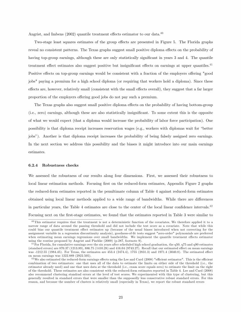
Angrist, and Imbens (2002) quantile treatment effects estimator to our data.40

Two-stage least squares estimates of the group effects are presented in Figure 5. The Florida graphs

reveal no consistent patterns. The Texas graphs suggest small positive diploma effects on the probability of

having top-group earnings, although these are only statistically significant in years 3 and 4. The quantile

treatment effect estimates also suggest positive but insignificant effects on earnings at upper quantiles.41

Positive effects on top-group earnings would be consistent with a fraction of the employers offering "good

jobs" paying a premium for a high school diploma (or requiring that workers hold a diploma). Since these

effects are, however, relatively small (consistent with the small effects overall), they suggest that a far larger

proportion of the employers offering good jobs do not pay such a premium.

The Texas graphs also suggest small positive diploma effects on the probability of having bottom-group

(i.e., zero) earnings, although these are also statistically insignificant. To some extent this is the opposite

of what we would expect (that a diploma would increase the probability of labor force participation). One

possibility is that diploma receipt increases reservation wages (e.g., workers with diplomas wait for “better

jobs”). Another is that diploma receipt increases the probability of being falsely assigned zero earnings.

In the next section we address this possibility and the biases it might introduce into our main earnings

estimates.

6.2.4 Robustness checks

We assessed the robustness of our results along four dimensions. First, we assessed their robustness to

local linear estimation methods. Focusing first on the reduced-form estimates, Appendix Figure 2 graphs

the reduced-form estimates reported in the penultimate column of Table 4 against reduced-form estimates

obtained using local linear methods applied to a wide range of bandwidths. While there are differences

in particular years, the Table 4 estimates are close to the center of the local linear confidence intervals.42

Focusing next on the first-stage estimates, we found that the estimates reported in Table 3 were similar to

40This estimator requires that the treatment is not a deterministic function of the covariates. We therefore applied it to a

narrow range of data around the passing threshold and did not include the test score as a covariate. Note that while this

could bias our quantile treatment effect estimates up (because of the usual biases introduced when not correcting for the

assignment variable in a regression discontinuity analysis), goodness-of-fit tests suggest "zero-order" polynomials are preferred

when estimating mean earnings regressions over small bandwidths. We implement the quantile treatment effects estimator

using the routine proposed by Angrist and Pischke (2009) (p.287, footnote 9).41For Florida, for cumulative earnings over the six years after scheduled high school graduation, the q50, q75 and q90 estimates

(standard errors) are 870.37 (1213.89), 886.75 (1410.28) and 416.04 (9743.27). Recall that our estimated effect on mean earnings

was -1212.55 (1984.45). For Texas, the estimates are 453.4 (2474.4), 1755 (2831.3) and 1971.4 (3040.8). The estimated effect

on mean earnings was 1222.889 (2922.505).42We also estimated the reduced-form earnings effects using the Lee and Card (2008) "efficient estimator". This is the efficient

combination of two estimators: one that uses all of the data to estimate the limits on either side of the threshold (i.e., the

estimator already used) and one that uses data at the threshold (i.e., exam score equals zero) to estimate the limit on the right

of the threshold. These estimates are also consistent with the reduced-form estimates reported in Table 4. Lee and Card (2008)

also recommend clustering standrad errors at the level of test scores. We experimented with this type of clustering, but this

generally resulted in standard errors that were smaller than the supposedly less conservative robust standard errors. For this

reason, and because the number of clusters is relatively small (especially in Texas), we report the robust standard errors

23

local linear estimates based on narrow bandwidths (which were suggested by cross-validation methods), but

not wider bandwidths. This is because a linear specification will not capture the curvature of the diploma-

score relationship to the left of the passing threshold (Figure 1). Overall, we conclude that local linear

estimates point to similar conclusions, at least when based on sensible bandwidths.

Second, we assessed whether our estimates could be biased by diploma effects on the probability that

workers are falsely assigned zero earnings (i.e., in non-covered employment, working for the federal govern-

ment, working out of state). This is a particular concern for Texas, since we found positive, albeit statistically

insignificant, diploma impacts on the probability of having zero earnings. It is also a concern for Florida,

since our estimated zero diploma impact on positive earnings could reflect positive diploma effects on the

probability of false-zero earnings and negative diploma effects on the probability of true-zero earnings.

Without information on the reason for zero earnings, it is difficult to rule out false-zero effects com-

pletely. Perhaps the most important possibility is that false-zero effects are driven by diploma effects on the

probability of military enlistment. That is because the military has a large presence in Texas and because

the military accepts very few applicants who do not have a standard (i.e., non-GED) high school diploma.

Yet despite higher enlistment rates among men, our estimated earnings effects are not obviously lower for

men than for women, and not obviously lower for individuals from counties close to military bases than for

individuals less close to military bases.43 Moreover, we estimate that the AFQT scores of last-chance-sample

students would be below those required for the military, at least assuming a rough correspondence between

exit exam and Armed Forces Qualifying Test (AFQT) scores.44 A second explanation for false-zero effects

is diploma effects on the probability of leaving the state. Census-based analysis of mobility out of state

suggests, however, that mobility effects are likely small. Among those in the relevant age group that lived

in Florida (Texas) five years before the Census (but not at the Census), the fraction with a diploma was

only 1.6 (3.6) percentage points higher than the fraction without a diploma. Since this is likely an upper

bound on the causal effect of diploma status on mobility out of state, we expect it is unlikely a phenomenon

of first-order importance.45 A third explanation for false-zero effects is diploma effects on the probability

of working in the uncovered (i.e., black) economy or being self-employed. Again though, we might expect

43We defined students as living close to a military base if there was a military base located in their county or in an adjacent

county (about 39 percent of the sample). Proximity to military bases is likely correlated with enlistment rates, since enlistment

rates in an area are known to be correlated with the proportion of veterans in an area (Warner, Simon, and Payne (2003)). For

most years, the estimated diploma effects were larger in magnitude (though never statistically significant) for students from

counties near military bases.44The military accepts very few applicants below the 31st percentile of the national AFQT distribution (Angrist (1993)).

In contrast, the median initial-attempt score in the Texas last-chance sample is at the twelfth percentile of the full-sample

distribution.45Calculations based on the five percent 2000 Census PUMS. Sample restricted to (1) 23-24 year olds (who were aged 18-19

five years ago, roughly the age at which the last-chance exam is taken) and (2) US natives or no older than 14 when they

immigrated to US. We obtained similar results when we restricted the sample to workers that completed grade twelve but did

not enroll in college.

24

workers with a diploma to be less likely to work in the black economy and less likely to be self-employed.

Third, we assessed the robustness of our estimates to diploma effects on downstream education outcomes.

These included the probability of enrolling in high school beyond the last chance exam, the probability of

pursuing and earning a GED, college enrollment, college credit accumulation and college diploma receipt.

These results are explored in more detail in Martorell (2010); a selection are presented in Appendix Figures

3-T and 3-F. The bottom line here is that while diploma receipt has the expected positive effect on college

outcomes and the expected negative effect on high school and GED outcomes, the estimates are relatively

small and short-lived. For example, while we find clear evidence of positive diploma effects on college

enrollment in Year 1, there are no effects in Year 2. There is also no effect on college attainment measured

by college academic credits or college degree completion. While we find clear negative effects on GED receipt

(workers that earn a high school diploma are around ten percentage points less likely to receive a GED), the

resulting bias is likely small, even assuming there are large returns to a GED.46 Under the more reasonable

assumption that a GED is equivalent to a high school diploma, we can deal with GED-taking by redefining

the treatment to be "diploma or GED", re-analyzing the first stage (which will result in first stage estimates

around 0.1 lower) and rescaling the existing reduced-form estimates by these new first-stage estimates. Since

the existing reduced-form estimates are close to zero and often negative, two-stage least squares estimates

that take account of GED-taking will be little changed.

Fourth, we assessed whether our results could be biased by endogenous compliance (i.e., compliance

among individuals that anticipate low diploma returns). As noted above, since endogenous compliance

imparts different biases depending whether it is on the left or right of the passing threshold, it is not clear

in which direction any endogenous compliance biases will go. Nevertheless, we tested this hypothesis using

what we believe is our best proxy for anticipated diploma returns: labor market attachment at the time of

the last-chance exam, as measured by earnings in high school. Since we find no relationship between high

school earnings and compliance, we suspect that this is not a first-order concern.47

7 Interpretation and Discussion

Across both states and across various subgroups, we could not reject the hypothesis that the signaling value

was zero. When we pooled across years and combined estimates from the two states, we could reject signaling

46For example, using observational estimates of the return to a GED, we calculate that downstream GED effects will bias

down our estimated signaling values by no more than one percentage point. These observational estimates (around 10 percent)

are based on regressions of earnings on dummies for whether a GED was attempted successfully and whether it was attempted

unsuccessfully (the omitted category was workers that did not attempt a GED) using samples of workers that failed the

last-chance test and did not obtain a diploma.47For example, in Florida, when we cut the sample by earnings in the year before the last-chance test, the estimated diploma

effects (standard errors) are (in ascending order of earnings) 0.498 (0.019), 0.507 (0.025), 0.528 (0.024) and 0.514 (0.024). For

Texas, the estimates (standard errors) are 0.412 (0.015), 0.397 (0.021), 0.425 (0.021) and 0.421 (0.021).

25

values in excess of five or six percent. In this section we consider the generalizability of these findings and

discuss what factors might explain them.

7.1 Can we generalize from the last-chance sample?

Our estimates were based on the subset of academically marginal students that sat the last-chance exam.

Before considering the generalizability of these estimates, we note that they should be of interest whether

they generalize or not. That is because they can inform the evaluations of policies that improve high school

academic performance or change high school graduation standards. Consider, for example, a policy designed

to improve high school math performance (e.g., Goodman (2009)). Even if this policy had no impact on

productivity, there could be a private return to this policy provided it caused some treated students to obtain

a high school diploma and provided that a diploma had a positive signaling value for these students.48 Since

the subset of students whose diploma status was affected by this policy should be similar to the academically

marginal students in our last-chance sample, and since we showed that a diploma carried zero signaling value

for these students, our results suggest that this signaling interpretation can be ruled out.

In fact, we believe that our estimates will generalize to other populations. More specifically, we believe

that the three main generalizability concerns are rejected by the data. One concern is that firms might

observe the number of times that individuals have taken the exit exam. In that case, they will know that

last-chance sample workers have typically taken the exam many times, might infer that they form a fairly

homogenous group, and might offer similar wages whether or not workers eventually received the diploma.

But estimates of the wage return to passing the exam at the first attempt (versus passing on a second or

subsequent attempt) are close to zero, which suggests that firms do not observe this type of information. This

is also consistent with more direct evidence showing that hiring firms rarely obtain students’ high school

transcripts, where this information would be found. Our analysis of the Bay Area Longitudinal Surveys

(BALS) of firms (Maxwell (2004)) shows that a transcript is request in less than four perent of cases.49 ,50

A second concern is that estimates based on last-chance-sample workers might be unusually low because

these workers perform unusually routine jobs in which a high school diploma does not matter (i.e., in which

workers with high school diplomas are no more productive than workers without them). Yet the data reject

48 In the context of our theoretical framework, we think of this policy as an increase in . If 2 = 0, this will have no

impact on productivity (i.e., zero social return). But if 1 0, it would improve high school performance and cause some

students to obtain a diploma. The diploma can carry a positive signaling value even if 2 = 0 (operating through study cost

function — i.e., studying is cheaper for more-able individuals), hence this policy could have a positive private return even if it

had no productivity effect. An important assumption is that firms cannot observe who has been treated by the policy. See the

discussion in Weiss (1995) of the relationship between firm information and the signaling interpretations of education changes

caused by potentially observable factors such as quarter of birth.49A 1987 survey of small and medium-sized employers found that transcripts had been obtained for only 13.7% of the hires

with twelve or fewer years of school (Bishop (1988)).50An alternative interpretation is that firms observe the number of attempts and the exact score obtained on each attempt,

but we argue in the next section that firms are unlikely to observe all of this information.

26

at least two implications of this hypothesis. First, assuming jobs correspond to six-digit industries, we

find that last-chance sample workers do similar jobs to full-sample workers (Appendix Figure 4-F). Second,

assuming that regression-based estimates of the return to a high school diploma measure how well diploma

receipt predicts productivity, we find that a high school diploma is almost as good a predictor of productivity

among low-ability workers (defined by initial exam scores) as it is among workers in other parts of the ability

distribution. These findings, based on regression-based estimates similar to those reported earlier (but split

by initial exam score), also hold after we condition on completing twelfth grade and not attending college

(Appendix Table 1).51 This implies, consistent with the work of Tyler (2004a) and others, that a high

school diploma predicts earnings even for academically weak students. Like Tyler (2004a), we cannot say

whether this reflects a correlation between diploma status and productivity-enhancing non-cognitive skills

(e.g., punctuality, reliability and so on) or between diploma status and productivity-enhacing cognitive skills

(e.g., numeracy and literacy).

A third more subtle concern that emerges from the theoretical framework is that there might be a positive

correlation between the signaling value of the high school diploma and the productivity signal observed by the

firm (i.e., 0() 0). In that case, since last-chance sample workers will have unusually poor productivity

signals (because they are, generally, low-ability workers), the diploma will have an unusually low signaling

value for them. Yet there is no obvious connection between the productivity signals received by firms and

the signaling value of a high school diploma. Indeed, one might expect the signaling value of a high school

diploma to be highest for workers with extremely good or extremely bad productivity signals.52 As a partial

test of this prediction we estimated whether the signaling value of the diploma was larger for last-chance-

sample students with relatively low ability (i.e., from high-scoring districts) than it was for last-chance-sample

students with relatively high ability. Although we found no clear evidence in either direction, the results

at least suggest that there is no obvious connection between relative ability and the signaling value of the

diploma.53

To summarize, while our estimates are based on a relatively small group of academically marginal workers,

we think this is a policy-relevant group and we see no reason why the signaling value for these workers should

be lower than it is for other types of students. While it is difficult to provide more positive evidence in support

of small signaling values among other types of students (without other good sources of diploma variation),

our results are consistent with our reading of the data on employer hiring practices. For example, it seems

51As with the estimates reported in Table 2, the estimates reported in Appendix Table 1 are based on a "full-time" sample

of individuals with earnings in all four quarters. We obtain similar estimates when we include those with zero earnings.52The intuition is that diploma information is more informative conditional on extreme signals. This can be shown in the

case in which the joint distribution of productivity and productivity signals is bivariate normal and diploma status is a function

of productivity (i.e., high school performance measures productivity).53 In Florida, for both types of district, estimates are positive in some years, negative in others and statistically signficant in

none.

27

that few employers create job ads that specify that applicants must have a high school diploma.54

7.2 What might explain these findings?

Our results suggest that the signaling value of a high school diploma is likely smaller than was previously

thought. At the end of our theoretical framework, we noted that three factors would reduce the signaling

value of the diploma: the availability of other sources of productivity information, the potential for diploma

misreporting and the availability of exit exam scores. We find the third explanation implausible. As noted

above, the data suggest that firms rarely ask for high school transcripts. In addition, in searching online job

ads and candidate resumes in Florida (on Monster.com), we were unable to find any that mentioned these

scores.

Instead, we suspect that our findings can be explained by a combination of the first two factors. That is,

we suspect that our discontinuity-based estimates are smaller because we suspect that the diploma has much

less predictive power for earnings conditional on all of the non-education productivity information held by

firms. Even at the point of hiring, it seems reasonable to suppose that firms observe a lot of non-education

productivity information. This could be obtained from resumes, letters of recommendation and, especially,

interviews and performance tests. It could also be provided in the process of job referral. Analysis of the

BALS data reveals that references are required for 80 percent of the positions filled and employment tests

for 22 percent of the positions filled; employer referrals are the most common means by which positions

are filled. Moreover, what firms do not observe at the time of hiring they might observe shortly afterwards

(Farber and Gibbons (1996), Altonji and Pierret (2001) and Lange (2007)).

The information content of a diploma will be further weakened by any misreporting of diploma status.

This is possible, since diploma information is likely difficult to verify. Firms could ask applicants to provide

a copy of their diploma, but applicants could claim to have lost their diploma or could provide a forged

diploma. Only by contacting an applicant’s high school can a firm verify diploma status, and high schools

are under no legal obligation to cooperate.55 Even when they do, the information may be provided too

late to be of use to a hiring firm. For example, according to Bishop (1988), Nationwide Insurance, "one

of Columbus, Ohio’s most respected employers", obtained permission to get all high school records for its

applicants. It sent over 1,200 such records to high schools in 1982 and received only 93 responses.56 The

54 In the job ads database assembled by Bertrand and Mullainathan (2004), fewer than 1% of ads state that applicants are

required to have a high school diploma (almost 10% state that a college degree is required). The job ads comprise all employment

ads in specific categories of the Sunday editions of The Boston Globe and The Chicago Tribune. The categories were sales,

administrative support, and clerical and customer services. The ads were collected from July 2001 to January 2002 (Boston

Globe) and July 2001 to May 2002 (Chicago Tribune). Calculations based on data kindly supplied by Marianne Bertrand.55Under the Federal Education Records and Privacy Act (FERPA), a school can release "directory informa-

tion" on names, dates attended and degrees earned without the written consent of the applicant or employee

(www.ed.gov/offices/OM/fpco/ferpa/index.html).56As a partial test of whether firms’ apparent indifference to diploma receipt can be thought of as a rational response to the

28

incentive to verify is further weakened by expected worker tenure, which might be short. For example,

among workers in the Florida full sample that start a job in the first quarter of Year 6, only 70 percent still

work for that firm in the second quarter, only around 50 percent work for that firm in the third quarter and

only around 40 percent work for that firm in the final quarter. These numbers are slightly lower among the

last-chance sample and are in line with the empirical exit hazards documented by Topel and Ward (1992).57

8 Conclusion

It is difficult to determine whether various types of education act as signals of underlying ability. In this

paper we estimated the signaling value of one type of education: a high school diploma. Using an approach

that identifies the signaling value of a diploma under much weaker assumptions than those made in the

previous literature, we estimated the signaling value of the diploma to be much smaller than the raw earnings

difference between workers with and without a diploma and much smaller than the estimates produced by

regression-based approaches (used in the previous literature). We suspect the difference reflects productivity

information held by firms but not the econometrician. Once we condition on this (as our approach implicitly

does), the information content of the diploma is likely much lower, and will be further weakened by diploma

mis-reporting. Since similar considerations likely apply to other types of lower-level education (e.g., high

school GPA, grade dropped out of high school), our findings suggest that among workers without a college

degree, the signaling value of various indicators of educational attainment is likely much lower than was

previously thought. It is not clear that our findings speak to workers with a college degree. For them,

indicators of educational attainment (e.g., college GPA, college selectivity) may be better predictors of

productivity and may be more easily verified.

Ultimately, economists care about education-based signaling because it implies that the private return

to education could exceed the social return to education, the parameter of interest relevant to education

policy. A large body of research (summarized by Card (1999)) suggests that at the lower end of the education

distribution, the private returns to education (e.g., additional years of high schooling) are relatively high. Our

analysis suggests that in this part of the education distribution, education-based signaling is less important

than was previously thought. As such, it suggests that the social returns to these types of education may be

even higher than was previously thought.

costs and benefits of verifying diploma information, we investigated whether diploma receipt was correlated with firm size, as it

might be if it was cheaper for larger firms to verify diploma information. The results suggest that there are no diploma effects

on firm size, although it is possible that larger firms can also acquire non-education information (e.g., organize performance

assessments) more cheaply.57For the last-chance sample, the fractions remaining in quarters 2, 3 and 4 are 61.4, 53.2 and 43.2 (N=13,776). For the

last-chance sample, they are 66.7, 48 and 37.1 (N=925). The empirical exit hazards reported by Topel and Ward (1992) (e.g.,

Figure 1) show the hazard rate declining from roughly 0.3 to roughly 0.2 over the first year of tenure.

29

References

Abadie, A., J. Angrist, and G. Imbens (2002): “Instrumental Variables Estimates of the Effect ofSubsidized Training on the Quantiles of Trainee Earnings,” Econometrica, 70(1), 91—117.

Acemoglu, D., and J. Angrist (2000): “How Large are Human-Capital Externalities? Evidence fromCompulsory-Schooling Laws,” NBER Macroeconomics Annual, 15, 9—74.

Altonji, J., and C. Pierret (2001): “Employer learning and statistical discrimination,” Quarterly Journalof Economics, 116, 313—350.

Angrist, J. (1993): “The "Misnorming" of the U.S. MilitaryŠs Entrance Examination and Its Effect onMinority Enlistmentse,” University of Wisconsin, Institute for Research on Poverty, Discussion Paper

1017-93.

Angrist, J., and V. Lavy (1999): “Using Maimonides’ Rule To Estimate The Effect Of Class Size OnScholastic Achievement,” The Quarterly Journal of Economics, 114(2), 533—575.

Angrist, J., and S. Pischke (2009): Mostly Harmless Econometrics. Princeton University Press, Prince-ton, NJ.

Bedard, K. (2001): “Human Capital Versus Signaling Models: University Access and High School Drop-outs,” Journal of Political Economy, 190(4), 749—775.

Bertrand, M., and S. Mullainathan (2004): “Are Emily and Greg More Employable Than Lakishaand Jamal? A Field Experiment on Labor Market Discrimination,” American Economic Review, 94(4),

991—1013.

Betts, J. (1998): “The Impact of Educational Standards on the Level and Distribution of Earnings,”American Economic Review, 88(1), 66—76.

Bishop, J. (1988): “Employer Testing and Incentives to Learn,” CAHRS Working Paper Series 433, CornellUniversity ILR School.

Borjas, G. (2005): Labor Economics (Third Edition). McGraw-Hill, New York, NY.

Cameron, S., and J. Heckman (1993): “The Nonequivalence of High School Equivalents,” Journal ofLabor Economics, 11(1), 1—47.

Card, D. (1999): “The Causal Effect of Education on Earnings,” in Handbook of Labour Economics Volume3A, ed. by O. Ashenfelter, and D. Card. Elsevier, Amsterdam.

Costrell, R. (1994): “A Simple Model of Educational Standards,” American Economic Review, 84(4),

856—971.

Dee, T. S., and B. Jacob (2006): “Do High School Exit Exams Influence Educational Attainment orLabor Market Performance,” NBER Working Paper 12199.

Ehrenberg, R., and R. Smith (2009): Modern Labor Economics (Nineth Edition). Pearson, Boston, MA.

Farber, H., and R. Gibbons (1996): “Learning and wage dynamics.,” Quarterly Journal of Economics,111, 1007—47.

Florida Department of Education (2005a): Assistance to 11th and 12th Grade Students that Have Not Earned

Passing Scores on Grade 10 FCAT for 2004-2005 (available online).

Florida Department of Education (2005b): FCAT Handbook - A Resource for Educators (available online).

Goodman, J. (2009): “The Labor of Division: Returns to Compulsory Math Coursework,” mimeo, HarvardKennedy School.

30

Hungerford, T., and G. Solon (1987): “Sheepskin Effects in the Returns to Education,” Review ofEconomics and Statistics, 69, 175—177.

Imbens, G. W., and J. D. Angrist (1994): “Identification and Estimation of Local Average TreatmentEffects,” Econometrica, 61(2), 467—476.

Imbens, G. W., and T. Lemieux (2008): “Regression discontinuity designs: A guide to practice,” Journalof Econometrics, 142(2), 615—635.

Jaeger, D., and M. Page (1996): “Degrees Matter: New Evidence on Sheepskin Effects in the Returns toEducation.,” Review of Economics and Statistics, 77, 733—9.

Jepsen, C., P. Mueser, and K. Troske (2010): “Labor Market Returns to the GED Using RegressionAnalysis,” mimeo, University of Kentucky.

Lang, K., and D. Kropp (1986): “Human Capital vesus Sorting: The Effects of Compulsory AttendanceLaws.,” Quarterly Journal of Economics, 101(3), 609—624.

Lange, F. (2007): “The Speed of Employer Learning,” Journal of Labor Economics, 25(1), 1—35.

Layard, R., and G. Pschacharopoulos (1974): “The Screening Hypothesis and the Returns to Educa-tion.,” Journal of Political Economy, 82, 989—98.

Lee, D., and T. Lemieux (2010): “Regression Discontinuity Designs in Economics.,” Journal of EconomicLiterature, 48(2), 281—355.

Lee, D. S. (2008): “Randomized Experiments from Non-random Selection in U.S. House Elections,” Journalof Econometrics, 142(2), 675—697.

Lee, D. S., and D. Card (2008): “Regression Discontinuity Inference with Specification Error,” Journalof Econometrics, 142(2), 655—674.

Lofstrum, M., and J. Tyler (2007): “Modeling the Signaling Value of the GED with an Application toan Exogenous Passing Standard Increase in Texas,” IZA Discussion Paper No. 2953, IZA, Bonn.

Martorell, P. (2005): “Do High School Graduation Exams Matter? Evaluating the Effects of Exit ExamPerformance on Student Outcomes.,” Unpublished manuscript, UC Berkeley.

(2010): “The Impact of High School Exit Exams on High School Graduation and Persistence,”

mimeo, RAND.

Maxwell, N. L. (2004): “The Bay Area Longitudinal Surveys of Firms,” HIRE Center Discussion PaperD04-06-04.

McCrary, J. (2008): “Manipulation of the Running Variable in the Regression Discontinuity Design: ADensity Test,” Journal of Econometrics, 142(2), 698—714.

Park, J. H. (1994): “Estimation of Sheepskin Effects and Returns to Schooling Using he Old and the NewCPS Measures of Educational Attainment,” Princeton University Industrial Relations Section Working

Paper 717.

Riley, J. G. (1979): “Testing the Educational Screening Hypothesis.,” Journal of Political Economy, 87(5),s227—s252.

(2001): “Silver Signals: Twenty-Five Years of Screening and Signaling.,” Journal of Economic

Literature, 39(2), 432—478.

Spence, M. (1973): “Job market signaling.,” Quarterly Journal of Economics, 83, 355—79.

Spence, M. (2002): “Signaling in Retrospect and the Informational Structure of Markets,” AmericanEconomic Review, 92(3), 434—459.

31

Texas Education Agency (2003): Timeline of Testing in TEXAS (available online).

Topel, R. H., and M. P. Ward (1992): “Job Mobility and the Careers of Young Men,” Quarterly Journalof Economics, 107(2), 439—479.

Tyler, J. (2004a): “Basic Skills and the Earnings of Dropouts,” Economics of Education Review, 23(3),221—235.

Tyler, J., R. Murnane, and J. Willett (2000): “Estimating the Labor Market Signaling Value of theGED.,” Quarterly Journal of Economics, 115, 431—468.

Tyler, J. H. (2004b): “What is the Value of the GED to Dropouts Who Pursue the Credential?,” Industrialand Labor Relations Review, 57(4), 587—598.

Warner, J., C. Simon, and D. Payne (2003): “The Military Recruiting Productivity Slowdown: TheRoles of Resources, Opportunity Cost and the Tastes of Youth,” Defense and Peace Economics, 14(5),

329—342.

Weiss, A. (1983): “A Sorting-cum-Learning Model of Education.,” Journal of Political Economy, 91, 420—42.

(1995): “Human Capital vs. Signalling Explanations of Wages.,” Journal of Economic Perspectives,

9, 133—154.

Wolpin, K. (1977): “Education and Screening,” American Economic Review, 73, 949—958.

32

Appendix

In this appendix we describe in more detail the relevant institutions and data sources.

A: Florida

A.1: Exit exams and high school graduation requirements

Florida was the first state to make high school graduation contingent on passing an exit exam (in 1978).58

In 2001, by which time Florida had developed an accountability system based on FCAT tests in grades three

through ten, the HSCT was replaced by the grade ten FCAT.

The grade ten FCAT exams are offered in reading and mathematics.59 Students must pass both. In

general, all students enrolled in grade ten should take these exams.60 The exams contain multiple choice

items, gridded-response items and performance tasks.61 Raw scores are scaled using item response theory

methods. The scaled scores range from 100 to 500 and cover five pre-defined levels of achievement.62 To pass,

students need to perform at the second level. For students in tenth grade in 2000-2001 (i.e., took the exam

for the first time in spring 2001), the passing scores were 287 for reading and 295 for math. For students

in tenth grade from 2001-02 onwards (i.e., took the exam for the first time from spring 2002 onwards), the

passing scores were 300 in both subjects. Students and parents receive a four-page report describing their

exam performance. This lists the scores obtained, whether the student passed, the associated performance

levels and the scores required to obtain the various performance levels and to pass.

Students that fail one or both of these exams have numerous opportunities to retake them. Students need

only retake the exams they have not yet passed. Initially, these retakes took the same format as the initial

exam. Starting fall 2004, the retake format changed to include only multiple choice and gridded response

questions.63 Students in tenth grade in 2000-2001 (i.e., took the first exam in spring 2001) had five chances

to retake the exam: the fall of eleventh grade (October 2001), the spring of eleventh grade (February-March

2002), the summer of eleventh grade (June 2002), the fall of twelfth grade (October 2002) and the spring

of twelfth grade (February-March 2003). Students in tenth grade in 2001-2002 onwards had an additional

retake opportunity in the summer of grade 10. Since few students retake the exam in the summer of tenth

and eleventh grades, students typically have five chances to pass before the end of grade twelve. School

districts are required to give “intensive remediation” to seniors that have not yet received a passing score on

the FCAT. In practice, schools offer remediation to students before they reach their senior year. Students

are given performance reports after each retake.

To obtain a public high school diploma, students must meet the exam requirement, maintain a 2.0 GPA

and earn course credits in the required number and distribution. Some students that have met the other

graduation requirements but not passed the FCAT can be exempted from the FCAT and can receive a

diploma. Exemptions are provided for students with disabilities if the student’s IEP team determine in

the student’s senior year that the FCAT does not accurately reflect the student’s abilities. Starting May

2004, students with ACT/SAT scores above certain thresholds are also exempt from the FCAT requirement.

Students that have met the other graduation requirements but not passed the FCAT can receive a “Certificate

58This section draws heavily on several Florida Department of Education publications. These include Florida Department of

Education (2005b) and Florida Department of Education (2005a).59The reading exam is a 160-minute exam that assesses students’ reading comprehension. The test is composed of about 6-8

reading passages (informational or literary) with sets of 6-11 questions based on each passage. The math exam is a 160-minute

exam that assesses performance on five strands: (1) Number Sense, Concepts and Operations; (2) Measurement; (3) Geometry

and Spatial Sense; (4) Algebraic Thinking and (5) Data Analysis and Probability. Students are allowed to use calculators.60LEPt students can be exempted if they have received services in an LEP program for one year or less. An Exceptional

Student Education (ESE) student may be exempted if he has an Individual Education Plan (IEP) and meets certain criteria.61 In gridded-response items, students answer questions that require a numerical response and they mark their numerical

answers in response grids.62These are “little success with the content on the FCAT” (level 1), “limited success with the content on the FCAT” (level 2),

“partial success with the content on the FCAT” (level 3), “success with the content on the FCAT by answering most questions

correctly, except for the challenging questions” (level 4), “success with the content of the FCAT by answering most questions

correctly” (level 5).63This change was designed to reduce grading costs. The DOE claimed that the new format was aligned with the old

standards. Students will receive this if their IEP team determines that the FCAT accurately reflects the student’s abilities.

33

of Completion”.64

Students that have met the other graduation requirements but have not passed the FCAT and are not

able to receive an exemption can still obtain a diploma if they pass another administration of the FCAT after

grade twelve. Students can retake the FCAT in the summer of grade twelve or in the following academic year.

They can prepare for the FCAT by taking an additional semester or full year (“thirteenth year”) of high

school education or by taking remediation and FCAT preparation classes available at adult and community

colleges.

Students wishing to enroll in state universities must have a high school diploma and must have acquired

course credits in specific amounts and types. Students wishing to enroll in college credit courses at community

colleges must have a high school diploma or must have a certificate of completion and pass a college placement

test. Students that do not pass the college placement test are placed in college preparatory courses. Students

can enroll in adult education programs without a diploma or a certificate of completion.

A.2: Data

The Florida data used in this paper were provided by the Florida Education and Training Placement Infor-

mation Program (FETPIP), a unit within the Florida Department of Education. FETPIP follows students

from school into post-secondary education and into the labor market. The FETPIP data combine several

data files that are linked at the student level using identifying information such as the student’s name, date

of birth and social security number. Since the data were linked before they were provided to us, match rates

are unknown.

The Florida data consists of a base enrollment record matched to several other types of data. The base

enrollment record refers to the academic year in which a student was first enrolled in grade ten in a Florida

public school (defined to include charter schools but not private schools). Every individual in the Florida

data is therefore associated with a unique base enrollment record and we use this to define the cohort to

which the individual belongs. In particular, we define cohorts 1-4 to include individuals in grade ten in

2000-01, 2001-02, 2002-03 and 2003-04.

Several types of data are matched to this base enrollment record:

1. Subsequent enrollments in Florida public schools: These enrollment records (and the base enrollment

record) include school and grade details and time-varying student details such as free lunch status and

special education classification.

2. Demographic data: These include information on sex, month and year of birth and race. Race is

classified as White, Black, Hispanic, Asian, and other.

3. Grade 10 FCAT data: In principle, these include details of all grade ten FCAT attempts, including

dates and scores obtained on both the math and reading sections. For the first and second cohorts,

grade ten FCAT data are only available for spring exams and retakes (i.e., not for summer and fall

retakes). Since both the first and last-chance exams are administered in spring, this is not an important

constraint.

4. Awards data: These include details of all certificates and diplomas awarded to students. These data

include the type of diploma awarded (e.g., high school diploma) and further details of the route by

which it was obtained (e.g., met standard requirements, exempted from FCAT requirement).

5. Postsecondary enrollment and awards data: These are available for all students that attend state

community colleges (CCs) and state universities (SUs) in Florida. The data include enrollment and

awards files similar to those available at the high school level. We use the postsecondary information

to define variables including “semesters in CCs” and “semesters in SUS”.

6. Earnings data: These come from the Unemployment Insurance (UI) tax reports submitted to the

Florida Department of Revenue by employers covered by the state’s UI law. Covered employers are

required to report, on a quarterly basis, the wages paid to each employee in order to determine the

64Special education students that have met the other graduation requirements but not passed the FCAT can receive a “Special

Diploma for Students with Disabilities”.

34

firm’s tax liability. Wages will be reported for nearly all individuals working for earnings in Florida.

The major categories not covered will be those working in the informal sector, the self-employed and

those working in the military. For each individual in our data we have, for each quarter, earnings

information as provided by each employer. We sum this to obtain “total earnings in the quarter” and

deflate it to $2000 using the CPI-U series. For earnings data from 2008 and 2009 we have an employer

identifier. Using another FETPIP-provided file that provides the six-digit industry of each employer,

we use this to determine the industry of each employer. “Year 1” earnings are computed as the sum

of earnings received in Q4 of the year of the last chance test and Q1-Q3 of the following year. Annual

earnings for subsequent years are defined in a similar fashion.

B: Texas

B.1: Exit exams and high school graduation requirements

The Texas class of 1987 was the first subject to the state’s exit exam requirement.65 In 1990, changes in

state law prompted the adoption of a new, harder set of exams called the Texas Assessment of Academic

Skills (TAAS). The stated purpose of the TAAS was to assess “higher-order thinking skills and problem

solving” (Texas Education Agency (2003)).66

The exit-level TAAS consisted of three sections (reading, math, and writing) all of which had to be

passed to satisfy the testing requirement. The math and reading sections had 48 and 60 multiple choice

questions, respectively, and state law set the passing standard to be 70 percent. The writing section had a

multiple choice component (40 questions) and an essay component, which was scored on a four-point scale.

The score for the writing section was computed by summing the multiple choice items correct and ten times

the essay section, and a passing score was set to be 48.67 The tests are designed to be of equal difficulty

across administrations, but the passing standards are still adjusted to be equivalent to passing standard

on the first (Fall 1990) exam.68 Students receive a score report describing their performance on the exam.

It contains the scores received on the exam, the standard required to pass each section, and whether the

student satisfied the graduation requirement.

Students who failed their first attempt could retake the exam during a subsequent administration (stu-

dents only had to retake sections they did not pass on an earlier attempt). The timing of the initial exam

and retake administrations changed over the study period. Students in tenth grade in the spring of 1991 or

1992 first took the exam in the fall of eleventh grade. The 1993-1995 tenth grade cohorts began taking the

TAAS in the spring of tenth grade. Students in all cohorts could retake the exam during administrations

given in the fall, spring, and summer. Beginning with the 1992 tenth grade cohort, seniors who had not yet

passed could take the exam one more time before graduation during a special administration given in April

or May. Thus the number of chances to retake the exam before the end of twelfth grade (for students not

held back) increased from five (for students in the 1991 tenth grade cohort) to eight (for students in the

1993-1995 tenth grade cohorts). Texas law requires that districts provide remedial services for students who

fail the exam (but does not mandate specific interventions).

To receive the “minimum high school program” diploma (the easiest high school diploma to obtain),

students had to meet the exit exam requirement and earn a minimum number of course credits across a

required distribution of subject areas. Students could receive special education exemptions from the exit

exam (or certain sections of the exit exam) and still earn high school degrees. To receive an exemption,

a student’s admission, review, and dismissal (ARD) committee has to determine that the TAAS is not

an appropriate measure of their academic progress.69 In Texas during this period, about seven percent of

students received exemptions from at least one section of the exam.Martorell (2005) Unlike Florida, Texas

65This section draws on Texas Education Agency (2003).66 Students could also take course-specific exams called End-of-Course (EOC) exams to satisfy the testing requirement. The

first class for which the EOC exams could be a substitute for the TAAS was 1999 (they were not fully phased in until the fall

of 1998). Consequently, the EOC exam are not relevant for the period in this study.67A minimum score of 2 on the writing section was also necessary, which implied that a student could still fail the writing

section with a writing score of 48 or greater if they received a 1 on the essay and got 38 out of 40 (or more) items correct on

the multiple choice. In practice, very few students scored a 1 on the essay and correctly answered 38 or more multiple choice

items.68These adjustments are typically no more than plus or minus one correct answer.69An ARD committee is made up of teachers, parents, and individuals with expertise working with special education students.

35

does not offer a certificate of completion to students who completed all other graduation requirements aside

from the exit exam. Individual districts, however, can issue these.

Students that complete all other graduation requirements, but that fail the exam and do not receive an

exemption, can attempt the exam after they leave school. If they pass, they are awarded a diploma. To help

prepare to retake the TAAS, students who have not graduated are also eligible to enroll in school for all of

or part of an academic year following their twelfth grade year (a “thirteenth year”).

Texas does not have statewide admissions standards. However, we checked admissions requirements at

several two- and four-year public institutions and most require proof that students graduated from high school

(earned a GED degree). Colleges that do not impose these requirements often impose other requirements.

For instance, Austin Community College admits non-high school graduates who can demonstrate “skill

proficiencies that support an ability to benefit from college-level instruction.”

B.2: Data

The Texas data used in this paper come from the Texas Schools Project (TSP), a collection of administrative

records from various Texas state agencies. These permit a longitudinal analysis of individuals as they proceed

through high school and later as they enter college or the workforce.

For this study we used five cohorts of students, defined in terms of the year in which they first took

the exit exam. These include students who took the initial exam in eleventh grade in the fall of 1991 and

1992, and students who took the initial exam in tenth grade in the spring of 1993-1995. Assuming no grade

repetition, these correspond to the 1993-1997 graduation classes. The initial exam record forms the basis

for the sample, and for each student in the cohorts we examine, we merged in data from the following Texas

Education Agency (TEA) files:

1. Exam files. There are separate files for each exit exam administration. We used these to generate

longitudinal exam-taking histories through 2002. One important limitation is that only scores from

the spring 1998 administration are included in the 1997-1998 school year. Thus, we have incomplete

data on retakes in the year after the final cohort of students was in twelfth grade.

2. K-12 Enrollment files. The TSP contains annual enrollment files from 1990 through 2002. These files

include fields for school, grade level, special education status, limited English proficiency and economic

disadvantage status.

3. K-12 Attendance files. These contain data on six-week attendance periods (six per school year) starting

in 1993. These files contain the number of days a student attended a given school in each attendance

period.

4. GED files. These are annual files that contain GED scores for individuals who attended Texas public

schools and who earned a GED certificate through 2002. Beginning in 1995, records for all GED test

takers are included regardless of eventual passing status.

5. Graduation files. These are annual rosters of students receiving a high school diploma from a Texas

public school between 1992 and 2001. The data distinguishes between basic and more advanced diplo-

mas. Since the exit exam is a requirement for the most basic diploma, we do not make use of information

on degree type.

We also merged in data from the following Texas Higher Education Coordinating Board (TEA) files (all

files available 1990 — 2005):

1. Report 1. These files, created every semester, include basic information for students enrolled in Texas

colleges including the school, semester and year in which a student was enrolled.

2. Report 2. These files, created every semester, include information on admissions tests, remediation

status, placement exam results and academic credits attempted in each semester. Academic credits

are those that count toward a degree, and “attempted” credits refer to credits in courses in which a

student earns a grade (i.e., they did not drop out of the course) but did not necessarily pass.

36

3. Report 9. These are annual rosters of awards issued by public colleges in Texas. These files identify

the type of degree (associates degree or baccalaureate degree)

We also merged in data from Texas Workforce Commission Files (available 1990 through 2004 Q3).

These quarterly files contain earnings reported by employers covered by the state’s unemployment insurance

system. This is similar to that described for Florida. “Year 1” earnings are computed as the sum of earnings

received in Q4 of the year of the last chance exam and Q1-Q3 of the following year. Annual earnings for

subsequent years are defined in a similar fashion.

Records were linked across files using a unique scrambled student ID used by the TEA. Records were

linked across agencies (e.g., TEA to TWC matches) using scrambled Social Security Numbers (SSN). We

checked to see if records matched on the basis of scrambled student ID or SSN were in agreement on variables

such as gender and date of birth. In general, these fields were almost always in agreement.

37

Figure 1: Last-chance exam scores and diploma receiptF

LOR

IDA 0

.51

1.5

-100 -50 0 50

Density of last-chance scores

0.2

.4.6

.81

-100 -50 0 50

Diploma receipt and last-chance scores

TE

XA

S

Notes: Graphs based on the last-chance samples. See Table 1 and text. For Texas, dots are cell means. For Florida, dots are averages of bins defined over two test scores (….[-2,-1], [0,1],…). Lines are fourth-order polynomials fitted separately on either side of the passing threshold.

01

23

45

6

-30 -25 -20 -15 -10 -5 0 5 10 15

Density of last-chance scores

0.2

.4.6

.81

-30 -25 -20 -15 -10 -5 0 5 10 15

Diploma receipt and last-chance scores

Figure 2: Descriptive statisticsF

LOR

IDA

01

2

-200 -150 -100 -50 0 50 100 150 200

Distribution of initial scores (full and last-chance samples)0

.2.4

.6.8

1

-200 -150 -100 -50 0 50 100 150 200

Complete 12th grade and initial scores (full sample)

0.2

.4.6

.81

-200 -150 -100 -50 0 50 100 150 200

Diploma receipt and initial scores (full sample)

Notes: Graphs based on the full samples and the last-chance samples. See Table 1 and text. For Texas, dots are cell means. For Florida, dots are averages of bins defined over five exam scores (….[-5,-1], [0,4],…) The scores on the X-axis are the minimum scores achieved on the initial exam for the subsample with scores on both subtests (see Table 1 for the relevant descriptive statistics).

TE

XA

S

01

23

45

-40 -35 -30 -25 -20 -15 -10 -5 0 5 10 15

Distribution of initial scores (full and last-chance samples)

0.2

.4.6

.81

-40 -35 -30 -25 -20 -15 -10 -5 0 5 10 15

Complete 12th grade and initial scores (full sample)

0.2

.4.6

.81

-40 -35 -30 -25 -20 -15 -10 -5 0 5 10 15

Diploma receipt and initial scores (full sample)

Figure 3: Earnings by last-chance exam scoresF

LOR

IDA

3000

700

0

-100 -50 0 50

Year 1

4000

800

0

-100 -50 0 50

Year 2

5000

9000

-100 -50 0 50

Year 3

5000

1000

0

-100 -50 0 50

Year 4

500

010

000

-100 -50 0 50

Year 5

5000

1000

0

-100 -50 0 50

Year 6

Notes: Graphs based on the last-chance samples. See Table 1 and text. For Texas, dots are cell means. For Florida, dots are averages of bins defined over two test scores (….[-2,-1], [0,1],…). Lines are fourth-order polynomials fitted separately on either side of the passing threshold. For Texas, "Year 2" exlcuded to conserve

TE

XA

S

3500

6000

-30 -25 -20 -15 -10 -5 0 5 10 15

Year 1

6000

1000

0

-30 -25 -20 -15 -10 -5 0 5 10 15

Year 3

6000

1200

0

-30 -25 -20 -15 -10 -5 0 5 10 15

Year 4

6000

1200

0

-30 -25 -20 -15 -10 -5 0 5 10 15

Year 5

6000

1400

0

-30 -25 -20 -15 -10 -5 0 5 10 15

Year 6

8000

1600

0

-30 -25 -20 -15 -10 -5 0 5 10 15

Year 7

Figure 4: Earnings effects by subgroup and year after last-chance exam (X-axis)F

LOR

IDA

-20

20

1 2 3 4 5 6

Main

-202

0

1 2 3 4 5 6

Male

-20

20

1 2 3 4 5 6

Female

-20

20

1 2 3 4 5 6

White

-20

20

1 2 3 4 5 6

Nonwhite

Notes: Graphs based on last-chance samples. See Table 1 and text. The solid lines connect 2SLS estimates of the diploma effect on earnings in each year after last-chance exam (i.e., the estimates reported in the final column of Table 4). The dashed lines connect points equal to these estimates plus and minus two times the associated standard errors. Estimates are expressed as a percentage of mean earnings in that year among individuals with an last-chance exam score of -1.

TE

XA

S

-20

020

1 2 3 4 5 6 7

Main

-20

020

1 2 3 4 5 6 7

Male

-20

020

1 2 3 4 5 6 7

Female

-20

020

1 2 3 4 5 6 7

White

-20

020

1 2 3 4 5 6 7

Nonwhite

Figure 5: Probability of earnings being in particular groupF

LOR

IDA

-.05

.05

0 1 2 3 4 5 6 7 8 9

Year 1

-.05

.05

0 1 2 3 4 5 6 7 8 9

Year 2

-.05

.05

0 1 2 3 4 5 6 7 8 9

Year 3

-.05

.05

0 1 2 3 4 5 6 7 8 9

Year 4

-.05

.05

0 1 2 3 4 5 6 7 8 9

Year 5

-.05.

050 1 2 3 4 5 6 7 8 9

Year 6

Notes: Graphs based on the last-chance samples. See Table 1 and text. Solid and dashed lines represent 2SLS estimates and associated confidence intervals, as in Figure 4. Group 0 corresponds to zero earnings. Groups 1-9 are equal-sized cuts of the conditional-on-positive earnings distribution. In Florida, the fractions with zero earnings in years 1 through 6 are 0.271, 0.280, 0.308, 0.324, 0.348 and 0.377. In Texas, the fractions with zero earnings are 0.2 in years 1-4, 0.21 in years 5-6, and 0.22 in year 7. For Texas, "Year 2" excluded to conserve space.

TE

XA

S

-.1

.1

0 1 2 3 4 5 6 7 8 9

Year 1

-.1

.1

0 1 2 3 4 5 6 7 8 9

Year 3

-.1

.1

0 1 2 3 4 5 6 7 8 9

Year 4

-.1

.1

0 1 2 3 4 5 6 7 8 9

Year 5

-.1

.1

0 1 2 3 4 5 6 7 8 9

Year 6

-.1

.1

0 1 2 3 4 5 6 7 8 9

Year 7

Appendix Figure 1: Routes to a diploma for students that fail the last-chance examF

LOR

IDA 0

.2.4

.6.8

1

-100 -50 0

High School Diploma (HSD)

0.2

.4.6

.81

-100 -50 0

Special Education (SE)

0.2

.4.6

.81

-100 -50 0

SE=1: HSD (solid), Passed after LCE (dash)

0.2

.4.6

.81

-100 -50 0

SE=0: HSD (solid), Passed after LCE (dash)

TE

XA

S

Notes: Florida graphs based on last-chance sample. Texas graphs based on last-chance sample excluding the final (10th grade in 1995) cohort. The final cohort is excluded because the testing data for the 1997-98 year are incomplete (this is the year after this cohort's last-chance exam). See Table 1 and text. Dots and lines as in Figure 1. Bottom-left (bottom-right) graph refers to those (not) classified as special education. "LCE" refers to last-chance exam.

0.2

.4.6

.81

-30 -25 -20 -15 -10 -5 0

High School Diploma (HSD)

0.2

.4.6

.81

-30 -25 -20 -15 -10 -5 0

Special Education (SE)

0.2

.4.6

.81

-30 -25 -20 -15 -10 -5 0

SE=1: HSD (solid), Passed after LCE (dash)

0.2

.4.6

.81

-30 -25 -20 -15 -10 -5 0

SE=0: HSD (solid), Passed after LCE (dash)

Appendix Figure 2: Local linear estimates relative to preferred estimates (dashed line)F

LOR

IDA

-10

10

0 10 20 30 40 50

Year 1

-10

10

0 10 20 30 40 50

Year 2

-10

10

0 10 20 30 40 50

Year 3

-10

10

0 10 20 30 40 50

Year 4

-1010

0 10 20 30 40 50

Year 5

-101

00 10 20 30 40 50

Year 6

TE

XA

S

Notes: Graphs based on last-chance samples. See Table 1 and text. The solid lines connects reduced-form estimates (dashed lines +/- two standard errors) for the symmetric bandwidth defined by the point at the x-axis (e.g., the estimates corresponding to x=10 are based on exam scores in the [-10,10] interval. The dashed horizontal line is the preferred reduced-form estimate (i.e., the estimate in column (5) of Table 4). For Texas, "Year 2" excluded to conserve space.

-50

5

5 10 15 20 25 30

Year 1

-50

5

5 10 15 20 25 30

Year 3

-50

5

5 10 15 20 25 30

Year 4

-50

5

5 10 15 20 25 30

Year 5

-50

5

5 10 15 20 25 30

Year 6

-50

5

5 10 15 20 25 30

Year 7

Appendix Figure 3-F: Postsecondary outcomes in Florida

Appendix Figure 3-T: Postsecondary outcomes in Texas

Notes: Graphs based on the 2000 cohort of the last-chance sample. See Table 1 and text. Dots are averages of bins defined over two test scores (….[-2,-1], [0,1],…). Lines are fourth-order polynomials fitted separately on either side of the passing threshold. The lines refer to the number of semesters enrolled in community colleges (CC) and the state university system (SUS) after the last-chance exam. For this cohort we observe post-secondary information for four years after the last-chance exam.

Enroll Yr 1 Enroll Yr 2

01

23

-100 -50 0 50

Semesters in CC(solid) and SUS(dash)

Note: Graphs based on the last-chance sample. See Table 1 and text. Dots are exam score cell averages. Lines are fourth-order polynomials fitted separately on either side of the passing threshold. Estimated discontinuities (using a fully-interacted quadratic in the test score) are: 0.086 (se=0.010) for enrolled in college in Year 1, 0.005 (se=0.010) for enrolled in college in Year 2, 0.332 (se=0.677) for total college academic credits, and -0.062 (se=0.005) for receive GED degree. We observe post-secondary information for these cohorts for seven years after the last-chance exam. 2SLS estimates of diploma impacts on these outcomes would be roughly 2.5 times as large.

0.1

.2.3

.4.5

-30 -25 -20 -15 -10 -5 0 5 10 15

Enroll Yr. 1

0.1

.2.3

.4.5

-30 -25 -20 -15 -10 -5 0 5 10 15

Enroll Yr. 2

05

10

15

20

25

-30 -25 -20 -15 -10 -5 0 5 10 15

College Academic Credits

0.0

4.0

8.1

2

-30 -25 -20 -15 -10 -5 0 5 10 15

Receive GED

Appendix Figure 4-F: Industry shares in Florida: full sample (Y) v last-chance sample (X)

Professional, technical & scientificPublic AdminstrationConstruction

Wholesale tradeTransportation & warehousing

Unclassified

Accomodation & food services

Health care & social assistance

Administration, etc

Retail trade

0.0

5.1

.15

.2

0 .05 .1 .15 .2

Two-digit industry

Full service restaurantsProfessional employer orgns

Unclassified

.06

.09 Six-digit industry

Notes: Graphs based on 2000 cohort (full sample and last-chance sample) with positive earnings in the first quarter of Year 6 (after the last-chance exam). See Table 1 and text. Industry refers to industry of main employer in first quarter of sixth year after the last-chance exam. Industries defined using NAICS 2002 classification. "Adiminstration, etc" in top panel is "Administrative and Support and Waste Management and Remediation Services".

Temporary help services

Warehouse clubs and supercenters

General medical and surgical hospitals

Limited service restaurants

General warehousing and storage

0.0

3

0 .03 .06 .09

Table 1: Descriptive statistics

Full sampleAll Fail Pass

Sample size 600,462 51,626 39,723 11,903 Coeff SEDemographics: Male 0.487 0.442 0.440 0.449 -0.019 0.015

Black 0.210 0.444 0.461 0.387 -0.010 0.015Hispanic 0.202 0.267 0.265 0.272 0.005 0.013

Free or reduced price lunch 0.279 0.479 0.497 0.421 -0.025 0.015Limited english proficient 0.187 0.337 0.346 0.305 -0.010 0.014

Special education 0.089 0.204 0.226 0.131 -0.004 0.010At grade level (initial attempt) 0.761 0.681 0.667 0.726 -0.023 0.015

Cohort 1 (grade 10 in 2000) 0.220 0.181 0.168 0.225 -0.013 0.012Cohort 2 (grade 10 in 2001) 0.240 0.270 0.248 0.343 0.010 0.014Cohort 3 (grade 10 in 2002) 0.265 0.258 0.261 0.250 -0.003 0.013Cohort 4 (grade 10 in 2000) 0.275 0.291 0.324 0.182 0.006 0.012

Initial exam: Took All Sections 0.976 0.976 0.976 0.974 0.004 0.004Reading (mean,sd) 7.7 (56.1) -54.9 (40.2) -60.2 (40.6) -37.3 (33.3) -0.434 1.015

Math(mean,sd) 23.3 (46.4) -24.3 (38.3) -27.9 (39.8) -12.2 (29.9) 0.819 0.926Pass (%) 0.570 0 0 0

Total exam attempts in HS: 1.723 4.422 4.498 4.168 0.009 0.0394Predicted earnings 28,548 28,140 27,357 30,754 -62.814 300.838

Full sample

All Fail PassSample size 777,892 37,571 23,242 14,329 Coeff SEDemographics: Male 0.487 0.421 0.416 0.430 -0.020 0.012

Black 0.117 0.246 0.256 0.230 -0.003 0.010Hispanic 0.289 0.478 0.505 0.434 -0.001 0.012

Free or reduced price lunch 0.213 0.409 0.442 0.354 -0.004 0.012Limited english proficient 0.040 0.147 0.177 0.099 -0.011 0.008

Special education 0.034 0.034 0.040 0.024 -0.006 0.004At grade level (initial attempt) 0.770 0.541 0.494 0.617 -0.031 0.012Cohort 1 (grade 11 fall 1991) 0.177 0.356 0.296 0.453 -0.006 0.011Cohort 2 (grade 11 fall 1992) 0.174 0.156 0.179 0.120 0.006 0.009

Cohort 3 (grade 10 spring 1993) 0.214 0.185 0.189 0.179 -0.017 0.009Cohort 4 (grade 10 spring 1994) 0.211 0.157 0.180 0.120 0.009 0.008

Initial exam: Took All Sections 0.949 0.956 0.956 0.955 -0.004 0.005Reading (mean,sd) 0.9 (11.7) -14.9 (7.9) -16.4 (7.7) -12.4 (7.4) 0.021 0.021

Math(mean,sd) 3.8 (7.5) -5.7 (6.8) -7 (6.9) -3.7 (6.2) -0.005 0.021Pass (%) 0.514 0 0 0

Total exam attempts in HS: 2.050 5.727 5.830 5.559 -0.008 0.030Predicted earnings Year 1-7 70,438.2 66,305.5 64,984.6 68,448.2 -323.194 328.563

TEXAS

Notes: See text for further description of full and last-chance samples. Last two columns report the estimated coefficients (and robust standard errors) on a "pass" dummy variable in regressions of these variables on the pass dummy and a third-order polynomial (Florida) or second-order polynomial (Texas) in the last-chance exam scores (interacted with the pass dummy). The final row refers to the fitted values from a regression of cumulative earnings in the six years (Florida) or seven years (Texas) after the last-chance exam on all of the demographics in the first panel, initial reading and math scores (missing values set to zero) and dummies for which sections were taken as part of the last-chance exam. This is the standard set of covariates used in the paper.

Last-chance sampleDisc

FLORIDA

Last-chance sampleDisc

Table 2: Regression-based estimates of the signaling value of a diploma

(1) (2) (3) (4) (5)

Diploma 2,694.7 2,687.2 2,686.4 3,297.4 2,119.2(226.1) (177.6) (196.7) (476.0) (438.8)

Demographics X XTest score XN 56,900 56,900 17,780 5,462 5,338Mean w/o HSD 17,627.8 17,627.8 15,979.9 18,873.1 18,729.9Diploma effect (%) 15.3 15.2 16.8 17.5 11.3

(1) (2) (3) (4) (5)

Diploma 4731.5 4129.2 3139.5 3975.6 3188.4(56.5) (55.4) (99.1) (275.2) (275.0)

Demographics X XTest score XN 432,222 432,222 180,972 47,777 47,777Mean w/o HSD 21,790.8 21,790.8 21,248.0 26,620.5 26,620.5Diploma effect (%) 21.7 18.9 14.8 14.9 12.0

White male only

Notes: Tables based on full samples. See Table 1 and text. First row reports estimates (second row reports robust standard errors) of the estimated coefficient on diploma receipt in regressions of earnings in the last year of the observation window (Florida: Year 6; Texas: Year 7) on diploma receipt and various controls. All models use only observations with positive earnings in every quarter of the relevant year. Estimates in columns (3)-(5) based on the subset of the full sample that complete twelfth grade and did not enroll in college. See text for further explanation. Demographic controls include sex, race and cohort dummies. Test score controls are scores on the initial attempt (with dummies for missing scores on a particular subject). The second-to-final row reports mean earnings among the subset of the relevant sample that did not earn a diploma. The final row reports the coefficient estimates as a percentage of this mean.

FLORIDA

Full sample Completed grade 12, no collegeTEXAS

Full sample Completed grade 12, no college

White male only

Table 3: Impact of passing the last-chance exam on the probability of earning a diploma

Poly-1 Poly-2 Poly-3 Poly-4 Poly-3+X

Pass 0.553 0.529 0.510 0.507 0.509(0.007) (0.010) (0.011) (0.012) (0.011)

Pass 0.548 0.519 0.498 0.495 0.499(0.008) (0.010) (0.011) (0.012) (0.011)

Pass 0.546 0.518 0.499 0.497 0.500(0.008) (0.009) (0.010) (0.011) (0.011)

Pass 0.545 0.484 0.481 0.475 0.486(0.007) (0.009) (0.012) (0.016) (0.009)

Pass 0.480 0.420 0.425 0.424 0.422(0.007) (0.009) (0.012) (0.016) (0.009)

Pass 0.472 0.415 0.419 0.417 0.417(0.007) (0.009) (0.012) (0.016) (0.009)

Pass 0.468 0.412 0.416 0.414 0.414(0.007) (0.009) (0.012) (0.016) (0.009)

Notes: Tables based on last-chance samples. See Table 1 and text. Cells report estimates (robust standard errors in parentheses) of the impact of passing the last-chance exam on diploma receipt. The column headings denote different exam score polynomials controlled for in these regressions (all interacted with a dummy for passing the exam). The final column presents estimates based on models that also control for covariates (see notes to Table 1).

Receive diploma within 1 year of last-chance exam (N=51,626)

Receive diploma within 2 years of last-chance exam (N=51,626)

Receive diploma within 1 year of last-chance exam (N=37,571)

Receive diploma within 2 years of last-chance exam (N=37,571)

Receive diploma within 3 years of last-chance exam (N=37,571)

FLORIDA

TEXAS

Receive diploma by end of summer of 12th grade (N=51,626)

Poly-1 Poly-2 Poly-3 Poly-4 Poly-2+X

Receive diploma before summer of 12th grade (N=37,571)

Table 4: Discontinuity-based estimates of the signaling value of a diploma

2SLS EstimatesPoly-1 Poly-2 Poly-3 Poly-4 Poly-3+X Poly-3+X

Pass/HSD -67.034 -51.506 -150.871 -221.647 -185.882 -372.115(80.506) (108.186) (127.240) (161.074) (134.172) (268.375)

Pass/HSD 24.142 -23.875 -257.322 -297.754 -286.701 -573.942(125.113) (183.936) (236.948) (278.897) (244.167) (488.308)

Pass/HSD 109.846 -52.121 -207.064 -74.161 -226.233 -452.893(157.231) (218.532) (276.025) (313.988) (283.406) (567.829)

Pass/HSD 107.069 -31.508 -164.844 10.325 -171.655 -338.086(184.994) (252.647) (306.313) (390.729) (324.031) (641.525)

Pass/HSD -327.268 -57.347 541.643 312.821 584.694 1186.428(449.648) (412.541) (420.181) (818.350) (436.215) (873.667)

Pass/HSD -860.494 -1105.003 -94.648 -270.329 -128.648 -256.265(595.864) (541.511) (505.279) (875.930) (493.726) (977.195)

Pass/HSD -46.998 -86.262 -103.401 -107.586 -123.873 -247.600(139.297) (170.221) (207.096) (267.951) (205.946) (411.829)

2SLS EstimatesPoly-1 Poly-2 Poly-3 Poly-4 Poly-2+X Poly-2+X

Pass/HSD -58.123 -26.765 -182.352 -209.524 -32.158 -77.126(100.732) (137.460) (173.737) (213.061) (134.500) (322.555)

Pass/HSD -2.754 39.427 -13.575 9.288 45.121 108.216(124.204) (169.980) (214.785) (263.331) (166.052) (398.262)

Pass/HSD 90.018 104.963 107.692 225.174 124.022 297.450(145.977) (197.152) (249.164) (303.060) (192.712) (462.258)

Pass/HSD 52.544 221.979 262.838 294.673 264.822 635.141(163.874) (219.469) (277.211) (336.630) (214.116) (513.727)

Pass/HSD -4.912 47.124 136.804 268.807 117.635 282.132(177.934) (240.035) (304.451) (373.857) (234.006) (561.234)

Pass/HSD 6.889 -52.730 -189.176 -80.987 34.183 81.983(198.010) (267.447) (337.067) (413.798) (260.499) (624.763)

Pass/HSD -24.726 -147.900 -192.856 16.023 -43.741 -104.906(213.279) (288.282) (361.694) (443.843) (280.866) (673.651)

Pass/HSD 8.420 26.585 -10.089 74.779 72.840 174.698133.399 180.113 227.229 277.775 174.074 417.501

Year 6 (Mean at score=-1: 9,794.0; N=9,336)

Reduced-Form Estimates

Year 1 (Mean at score=-1: 5,451.2; N=51,626)

Year 2 (Mean at score=-1: 7,267.1; N=51,626)

Year 3 (Mean at score=-1: 7,454.7; N=51,626)

Year 4 (Mean at score=-1: 8,389.5; N=36,604)

FLORIDA

Years pooled (Mean at score=-1: 8005.7; N=224,086, N(cluster)=51,626)

Years pooled (Mean at score=-1: 9580.2; N=262,997, N(cluster)=37,571)

Year 6 (Mean at score=-1: 12,355.1; N=37,571)

Year 7 (Mean at score=-1: 12,879.0; N=37,571)

Year 5 (Mean at score=-1: 8,653.5; N=23,268)

Notes: Estimates based on same samples/models as those reported in Table 3. Individuals with zero earnings included in these regressions. The bottom row reports estimates from models in which year-specific data are stacked and standard errors are clustered at the individual level.

Reduced-Form EstimatesTEXAS

Year 1 (Mean at score=-1: 5,529.2; N=37,571)

Year 2 (Mean at score=-1: 7,107.6; N=37,571)

Year 3(Mean at score=-1: 8,381.8; N=37,571)

Year 4 (Mean at score=-1: 9,783.4; N=37,571)

Year 5 (Mean at score=-1: 11,025.4; N=37,571)

Table 5: Restricted and combined estimates of the signaling value of a diploma

Year 1 Year 2 Year 3 Year 4 Year 5 Year 6 Year 7 Pooled

Unrestricted Coeff -372.11 -573.94 -452.89 -338.09 1186.43 -256.26 -247.60SE (268.37) (488.31) (567.83) (641.53) (873.67) (977.19) (411.83)Ub on CI 3.02 5.54 9.16 11.26 33.90 17.34 7.20

Restricted Coeff -76.69 -0.16 118.96 287.25 -304.66 -2254.7 -74.77SE (218.56) (272.41) (316.09) (375.86) (818.97) (1120.20) (283.47)Ub on CI 6.61 7.49 10.08 12.38 15.41 -0.15 6.15p-value 0.42 0.09 0.23 0.4 0.61 0.45 0.37

Unrestricted Coeff -77.13 108.22 297.45 635.14 282.13 81.98 -104.91 174.70SE (322.55) (398.26) (462.26) (513.73) (561.23) (624.76) (673.65) (417.50)Ub on CI 10.27 12.73 14.58 16.99 12.74 10.78 9.65 10.54

Restricted Coeff -57.06 78.29 338.22 305.66 169.70 -10.28 -92.53 104.57SE (258.82) (318.37) (375.04) (420.34) (453.53) (509.19) (551.39) (339.72)Ub on CI 8.33 10.06 12.98 11.72 9.77 8.16 7.84 8.18p-value 0.99 0.99 0.69 0.18 0.77 0.68 0.91 0.54

Unrestricted Coeff -251.442 -164.286 -1.61969 254.8875 546.2927 -16.1617 -39.34SE (206.30) (308.63) (358.49) (401.00) (472.20) (526.38) (293.19)Ub on CI 2.94 6.32 8.93 11.44 14.43 8.93 6.23

Restricted Coeff -68.5189 32.99776 210.0232 295.4299 58.36799 -394.618 -1.16SE (166.99) (206.98) (241.70) (280.18) (396.76) (463.55) (217.65)Ub on CI 4.84 6.21 8.84 9.50 8.14 4.47 5.02

FLORIDA

TEXAS

FLORIDA & TEXAS COMBINED

Notes: Tables based on last-chance samples. The “unrestricted” estimates are reproduced from Table 4. The “restricted” estimates are the ratio of reduced-form to first-stage estimates, where these are estimated separately, using separate specifications (standard errors calculated using the delta method). The first-stage specification uses a polynomial that is fully-interacted with the pass dummy. The reduced-form specification uses a polynomial that is not interacted with the pass dummy. The “Florida and Texas combined” estimates are weighted averages of the corresponding state-specific estimates. The associated standard errors are a function of the weights and the state-specific variance estimates. The weight on the Florida estimate is the Texas variance estimate as a proportion of the summed variance estimates.

Appendix Table 1: Regression-based estimates of the signaling value of a diploma: by ability

All Group 1 Group 2 Group 3 Group 4 Group 5 Group 6<-31 [-31,-2) [-2,18) [18,36) [36,56) >=56

HS diploma 2,687.22 1,025.73 2,025.35 1,962.70 1,808.08 2,562.86 3,142.76(177.64) (376.80) (241.85) (312.62) (352.15) (412.67) (640.02)

N 56,900 7559 9510 9495 10038 10029 8885Mean w/o diploma 17,627.8 17,106.9 17,039.6 18,177.5 18,800.4 18,618.7 19,757.6Diploma effect (%) 15.2 6.0 11.9 10.8 9.6 13.8 15.9

HS diploma 2,686.44 1,126.65 2,231.49 2,786.91 2,415.95 3,688.69 4,096.02(196.69) (310.78) (385.14) (598.35) (728.73) (960.22) (1748.06)

N 17,780 3780 4017 3296 2839 2082 1300Mean w/o diploma 16,979.9 16,781.2 16,852.7 17,487.5 17,971.4 17,853.0 20,356.8Diploma effect (%) 15.8 6.7 13.2 15.9 13.4 20.7 20.1

All Group 1 Group 2 Group 3 Group 4 Group 5 Group 6<-12 [-12,-5) [-5,1) [1,5) [5,9) >=9

HS diploma 4129.2 1944.1 1871.1 2287.7 2607.6 3383.2 3042.5(55.4) (85.1) (109.3) (129.6) (169.4) (204.7) (281.8)

N 432,222 71,182 65,697 77,309 64,200 72,366 62,779Mean w/o diploma 21,790.8 19,218.8 21,530.2 22,906.5 24,314.0 25,538.4 28,715.7Diploma effect (%) 18.9 10.1 8.7 10.0 10.7 13.2 10.6

HS diploma 3139.5 1414.8 1659.7 1825.8 2485.2 3176.3 3444.6(99.1) (129.4) (172.8) (231.1) (319.1) (422.7) (701.1)

N 180,972 37,394 40,323 41,801 30,307 26,841 20,584Mean w/o diploma 21,248.0 19,119.0 21,391.4 23,047.4 24,151.0 25,377.8 28,200.5Diploma effect (%) 14.8 7.4 7.8 7.9 10.3 12.5 12.2Notes: Table based on full samples. See Table 1 and text for more details. Bottom panel based on subset of full panel that complete twelfth grade and do not enroll in college. See text for more details. The cells report estimates (robust standard errors in parentheses) from models identical to those underlying Table 2 (see notes to Table 2 for more details). The first columns use all observations, hence estimates are identical to those reported in columns (2) and (3) of Table 2. The next six columns report estimates from models restricted to observations from six groups corresponding to 6-tiles of the minimum score on the initial exam (only observations with non-missing scores for all initial-attempt subjects included). The column headings describe the relevant score cutoffs. The second-to-final row reports mean earnings among the subset of the relevant sample that did not earn a diploma. The final row reports the coefficient estimates as a percentage of this mean.

Full Sample

Completed grade 12, no college

FLORIDA

TEXAS

Full sample

Completed grade 12, no college