Embed Size (px)
Citation preview

The role of optimization and simplified
methods in the design of Thermally
Activated Building Systems (TABS) Yueting Yang 0789016
7/25/2013
[1]
Supervisor:
prof. dr.ir J.L.M. Hensen
dr. D. Costola
/ Unit Building Physics & Services
/ Built environment department

Yueting Yang The role of optimization and simplified methods in the design of Thermally Activated Building Systems (TABS)

Contents
1. Introduction ............................................................................................................ 1
1.1 Background of TABS system ................................................................................... 1
1.2 Complexity of design ............................................................................................ 1
1.3 Focus on pipe level ............................................................................................... 2
1.4 Research question ................................................................................................ 2
2. Research methodology ............................................................................................... 3
2.1 Current TABS design method ................................................................................. 3
2.2 Simulation and optimization design method ................................................................ 4
2.3 Case study ......................................................................................................... 5
3. Result and discussion ................................................................................................. 7
3. 1 Optimization ..................................................................................................... 8
3.2 Design method................................................................................................... 13
4. Conclusion ............................................................................................................ 16
Appendix .................................................................................................................. 25
5. Heat transfer theory and modeling of TABS system in TRNSYS ............................................ 27
5.1 TABS modeling in TRNSYS .................................................................................. 27
5.2 Heat transfer theory of TABS in TRNSYS .................................................................. 27
6. Case study design in current methods ............................................................................ 29
6.1 Simplified sizing by diagrams in standard [60] ............................................................. 29
6.2 Straightforward unknown but bounded method (SUB) [65] ............................................ 31
6.3 Rehva guidebook [53].......................................................................................... 32
6.4 Design manual from manufacture in USA [49] ............................................................ 34
6.5 Design manual from manufacture in Canada [55] ......................................................... 39
7. Single pipe dimension optimization ............................................................................... 41
7.1 Simulation and modeling ...................................................................................... 41
7.2 Thermal demand and pipe dimension ....................................................................... 41
7.3 Overheating hours and pipe dimension ..................................................................... 45
7.4 Pareto front in single dimension optimization .............................................................. 46

Yueting Yang The role of optimization and simplified methods in the design of Thermally Activated Building Systems (TABS)

Yueting Yang The role of optimization and simplified methods in the design of Thermally Activated Building Systems (TABS)
Page 1
The role of optimization and simplified methods in the design of
Thermally Activated Building Systems (TABS)
YUETING YANG‡
Thermally Activated Building Systems (TABS) are widely used because of energy saving and improved indoor comfort.
There are some simplified design methods of TABS systems including European standards, manuals from scientific
institution and manufacture guidebooks. To figure out the optimal design method, simulation and optimization are
integrated as a new method. By defining objectives as energy saving and comfort improving, 4 kinds of optimization
are investigated regarding pipe dimension design and supply water design. In a case study, the pipe dimension design
and supply water design of current simplified methods and the new simulation integrated optimization method are
shown. The corresponding building performances under each design are compared to figure out the optimal solution.
1. Introduction
1.1 Background of TABS system
Active building components are thermally heavy
parts of the building construction, which are
equipped with ducts for circulation of air or
embedded pipes for circulation of water [2] (Figure
1). Buildings equipped with thermally activated
building systems (TABS) system are heavy thermal
mass constructions with high thermal inertia, which
could absorb more heat and solar gain in and delay
the heat transfer from outside to inside [2]. In this
way, indoor temperature could be kept within a
comfortable range regardless of wide fluctuation of
ambient temperature.
TABS has been widely used in modern building
design and develops towards more energy efficient
way [3-13]. As an adaptive design, TABS has been
investigated in various environment and integrated
with numerous systems, such as heat pump ground-
coupled system [14], combined cooling, heating &
power system (CCHP) [15] and rainwater system
[16]. In this process, energy consumption could be
reduced compared with conventional systems.
Another advantage of TABS system is it can satisfy
different indoor comfort levels by low energy
consumption [17], which reduces greenhouse gas
emission [18] and allows the utilization of low grade
energy sources, such as the ground [19-20], outside
air [21] or recovered process heat [22]. As a thermal
mass integrated with the whole building, TABS
system also functions well in peak shaving and time
lag due to its thermal inertia effect [8,22-27], which
brings economic benefits when exploiting the
nighttime cheap electricity tariff[18].
There are also some potential barriers and
limitations in application. TABS is only suitable for
buildings with low heating/cooling loads (
[2]. High thermal insulation of the building
envelope and proper solar shading is a prerequisite
for application [2]. Control strategy has influence
on TABS design and performance, but there are
various ways of control which cannot be
determined at the TABS design stage. In other
words, control and design of TABS are in circular
cause and consequence.
1.2 Complexity of design
Considering the benefits and limitations of TABS
systems, there are potentials and complexities in

Yueting Yang The role of optimization and simplified methods in the design of Thermally Activated Building Systems (TABS)
Page 2
the design process, which can be classified by three
levels.
Figure 1. Schematic diagram of Thermally Activated Building Systems (TABS) [28]
Building level
At building level, the designers deal with problem
related to TABS application rage and necessity.
Various building construction types [29], kinds of
climate environment and different comfort models
[30-32] should be taken into account. Once the
capacity of TABS can be decided, the necessity of
auxiliary equipment (solar panel, chiller etc.) can
also be known. The application of phase change
material also plays an important role in TABS
system [33-35].
System control level
The diverse control strategies of TABS can be
classified as water temperature control and pump
operational control (power control & energy
control). The control could be continuous or
discontinuous in a time step of one hour or one day.
Related researches cover topics including the
switching point between cooling and heating modes
[36-37], control efficiency [38-39], hydronic circuit
topologies [40-41] and integrated control with
occupant behavior [42-43].
Pipe level
There are many standards and guidebooks regarding
pipe design of TABS [44–60] which includes both
pipe dimension and supply water to pipes. Pipe
dimension design refers to sizing the pipes [61] such
as pipe diameter, pipe spacing, pipe wall thickness,
loop length and position of the pipes embedded in
the construction. Supply water design concerns
about designed heat loss, supply water
temperature, mass flow rate and pressure drop etc.
Given the heat transfer analysis and thermal
resistance model [62-63], the variables at pipe level
are directly related to the building performance.
1.3 Focus on pipe level
In most TABS design guidebooks, the supply water
design is determined based on the known pipe
dimension. The design methods discussed in this
passage come from European standard, scientific
organizations and manufactures. These current
methods are direct and straightforward, but also
less accurate and without optimal result because of
the assumptions about limited control strategies and
unstated hydronic configuration.
To set up more convincing guidelines and provide
optimal solutions, the method in this research
makes use of simulation and optimization. Modeling
and simulation have been widely used in building
performance prediction. Optimization is the
mathematical selection of a best element (with
regard to some criteria) from some set of available
alternatives to achieve defined objectives [64].
Combined optimization with simulation, a better
solution could appear in terms of TABS design.
1.4 Research question
Given the benefits of optimization, limitations of
existing design methods and more potentials of
TABS system, this research would investigate the
feasibility of optimization in design of
Thermally Activated Building Systems (TABS)
when compared with existing simplified
methods.
This passage will illustrate the research question in
the following parts. The research methodology
clarifies the current situation of existing design
methods and the integration method of
optimization and simulation. A case study has been

Yueting Yang The role of optimization and simplified methods in the design of Thermally Activated Building Systems (TABS)
Page 3
introduced to investigate the quantitative analysis of
each method. The design and performance are
compared to select the optimal design method.
2. Research methodology
2.1 Current TABS design method
2.1.1 Design method from European
standard [60]
2.1.1.1 Rough sizing method
Based on the assumption of operative temperature
as 24˚C, the cooling system can be sized for 70%
of the peak cooling load. Since the inaccuracy is
around 20~30% and there is no information about
supply water temperature or pipe dimension, this
rough sizing method can only be used to size the
production unit.
2.1.1.2 Simplified method using diagrams for sizing
Within the frame of assumed operation mode,
orientation and active surface, the linear
relationship of core temperature, daily heat gain,
total thermal resistance and circuit running time has
been set up to determine the supply water
temperature. This method is based on the
assumption that both the entire conductive slab and
supply water are at constant temperatures during
the whole day. The dis-advantage lies in the
limitation of operation mode, no dynamic
consideration and no instruction on sizing pipe
dimension, which leads to 15~20% inaccuracy.
2.1.1.3 Simplified model based on finite difference
method (FDM)
Based on the knowledge of 24 values of the variable
cooling loads of the room and the temperature of
the air, detailed dynamic simulation for thermal
conduction in the slab via FDM has been applied to
get the related surface and supply water
temperature (inaccuracy 10~15%). The pre-
requisite of application is that the operative
temperature of the room has to be 20˚C to 25.5˚ C
as the program underestimates the temperature of
the room. The following limitations should be met
(1) pipe distance ranges from 0.15 to 0.3m, (2)
usual concrete slab structure have to be considered,
, without discontinuous light
fillings in upper or lower slabs.
2.1.1.4 Dynamic building simulation program
By taking into account of the water flow into pipes,
the heat conduction between upward and
downward surface of the slab and the pipe level,
heat conduction of each wall, mutual radiation
between internal surfaces, convection with air and
the internal balance of the air, the detailed dynamic
building-system model has been carried out.
2.1.2 Design method from scientific
organization
2.1.2.1 Rehva guidebook using diagrams for sizing [53]
There are only two types of pipe dimension
available in this method: 0.15m and 0.3m for pipe
spacing. The relationship of heat exchange rate,
thermal resistance of floor covering and medium
differential temperature has been built up and can
be read from the diagram. But the result of medium
differential temperature does not shown the exact
value of supply water temperature, return water
temperature or indoor temperature. It only reveals
the rational result of these three temperatures.
(Equation 1)

Yueting Yang The role of optimization and simplified methods in the design of Thermally Activated Building Systems (TABS)
Page 4
2.1.2.2 Straight-forward unknown but bounded method
(SUB) [65]
In contrast to the conventional iterative design
method of TABS, which is based on iterative
dynamic model simulation studies, this approach is
a more straight-forward calculation process, which
is less time-consuming and enables more insight
into the potential of TABS. Based on estimated
lower and upper bounds for the heat gains, the
supply water temperature and control set-point can
be decided. It also shows the limitation of TABS
application and points out when additional auxiliary
heating or cooling devices have to be installed. The
assumption behind this method is the daily variable
heat gains has been transferred to equivalent bounds
based on a linear relationship. An outstanding
advantage of this method is that it distinguishes
ceiling and floor, heating and cooling.
2.1.3 Design method from manufacture
resource
2.1.3.1 Design and installation guide from manufacture
in USA [49]
Based on floor covering and designed heat output,
the supply water temperature and TABS dimension
can be sized. It serves for both residential and light
commercial buildings. The general diagrams are
provided for designers and installers to follow. But
it is obvious that the suggested supply water
temperature and heat output are quite high
compared with normal range.
2.1.3.2 Design and installation guide from manufacture
in Canada [55]
Similar to the design guide from manufacture in
USA, the method is also on the basis of floor
covering and designed heat output. The difference
is that flow rate in this method is an essential
variable in dimension parameters determination
instead of a result determined by dimension
parameters according to the design guide from
USA. This diminishes error propagation and
improves accuracy because there is more
uncertainty in sizing dimension than flow rate.
2.2 Simulation and optimization design method
2.2.1 Application of simulation in TABS
Over the past 30 years, the importance of building
simulation has become more and more obvious in
research about TABS system. The performance of
TABS is strongly related to the design details and
control strategy, which can be modeled in various
simulation software packages, such as ESP-r,
TRNSYS, IES VE, IDA ICE, & EnergyPlus [66]. By
means of computational simulation, design
complexities are investigated and possible
performance are predicted without time and money
wasted in uncertain construction. For example, it
was found that reductions up to 50% of the cooling
capacity for a chiller can be achieved using TABS
[25,67].
2.2.2 Application of optimization in
simulation
In order to achieve optimal system performance
under some architectural and comfort constraints,
the optimal sets of design parameters in building
envelope and HVAC system play an important role
[68-69]. In other words, optimization techniques
aim to solve problems in a systematic way by
producing a set of solutions based on predefined
objectives that are functions of design variables [70].
In the literature [71], savings of 5% to 30% in
annual energy consumption for lighting, cooling
and heating due to optimized building and HVAC
design has been reported.
The most common optimization theory is Genetic
Algorithm(GA) [72]. Its popularities comes from
the easiness of implementation since it can take into

Yueting Yang The role of optimization and simplified methods in the design of Thermally Activated Building Systems (TABS)
Page 5
account discontinuous design parameters instead of
smoothing the approximating objectives. And its
population-based search has an advantage in multi-
criteria optimization decision making, which elicits
the specific optimization technique used in this
passage—multi-objective genetic algorithm
(MOGA). The obvious characteristics of this
method is to treat constraints as criteria and force
solution into desired feasible region(by penalizing
Pareto rank of infeasible solutions) [73].
2.2.3 Combined design of simulation and
optimization
In this paper, the simulation and optimization are
well combined to investigate the guidelines for
TABS designers. The methodology is shown in
Figure 2.
Figure 2 Integration schematics of optimization and simulation
A case study has been built up in TRNSYS, in which
the building with TABS system in case study has
been modeled and simulation results of energy and
comfort are available.
Optimization and simulation have been integrated
on the platform of modeFrontier. Some design
variables in TRNSYS model can be re-defined as
inputs (pipe dimension and supply water variables)
and some simulation results can be selected as
outputs (energy and comfort). The selection of
input values is made by Design of experiments
(DOE), which enables the number of designs and
the content of the sequence can be defined by the
user. The scheduler is based on the user’s sequence
defined in the DOE table. The outputs can be
related to objectives either maximize or minimize
the value. By clarifying objectives, the optimization
method—multi-objective genetic algorithm
(MOGA) is applied to help inputs selection in
purpose of driving the corresponding outputs
towards objectives.
2.3 Case study
2.3.1 Location and basic building
information
The building called Hollandsch Huys in case study
(Figure 3) is a 5-storeis multi-functional building
located in the city of Hasselt, Belgium.
Figure 3 Building in case study--Hollandsch Huys
The TABS system embedded in both floor and
ceiling for heating and cooling, which integrated
with air handling unit as the HVAC system. TABS
system has been simplified modeled using an
equivalent 1D model with one pipe instead of 3D
model, which is based on the work of (Wout Parys
and Dirk Saelens, 2001) [74]. The model is
subdivided in 12 thermal zones based on the layout
of pipes in the TABS system. The spatial indoor
comfort level is also measured by the overheating
and underheating hours in each thermal zone.
Zone 1 (Figure 4) has been selected for case study
but the whole building with system has been
modeled. It is located on the first floor of the
building and more detailed information is listed in
Table 1.
2.3.2 Control strategy

Yueting Yang The role of optimization and simplified methods in the design of Thermally Activated Building Systems (TABS)
Page 6
2.3.2.1 Top level control
Top level control decides the running mode of the
system which relates to the convective heat transfer
coefficient in TABS (Table 2). According to the
average ambient temperature, three modes of
TABS can be specified including heating mode, free
running mode and cooling mode. The supply water
temperature set points depend on the average
ambient temperature during the six previous hours,
as shown in Figure 5.
Figure 4 Zone 1 in case study
Table 1 Detailed construction and system information of Zone1
Table 2 Operation mode control scheme
Figure 5 Supply water temperature control scheme in reference case
2.3.2.2 supply water mass flow rate control
As shown in Table 1, supply water mass flow rate is
decided by both water scheme and occupied area.
The hourly water scheme can be divided into two
time periods. The water is supplied to the building
in the first 10min of each hour, and the later water
scheme is decided by the temperature difference of
inlet and outlet TABS water at the 10th min. If the
temperature difference is more than 2˚C, the water
should be delivered to the building in the rest 50
minutes, otherwise TABS system would stop water
supply.
2.3.4 Simulation setting (Trnsys)
Typical week:
typical summer week: 4837~5004 hr (July)
typical winter week: 169~336 hr (January)
Time step: 2 min
2.3.3 Optimization setting (modeFrontier)
Input variables
The input variables at pipe level can be divided into
pipe dimension and supply water variables (Table
3). The supply water temperature can be a constant
value during the simulation time or follow a new
linear supply water –ambient temperature
relationship (Figure 6).
Space length, width, height 6.76m*6.95m*2.7m
Façade South/East
18.66/19.18 m2
0.205W/(m2•K)
41.27%
Adjacent wall West/North
18.66/19.18 m2
4.082 W/(m2•K)
Floor/Ceiling 46.98 m2
1.692 W/(m2•K)
weather BE_Brussels-National-64510.tm2
occupancy occupant density 10 m2/occupant
occupancy schedule Monday to Friday
8:00 am-18:00 pm
computer power 140 w
number occupant number
artificial lighting 10 w/m2
Infiltration 0.5 ACH
Solar radiation calculated from weather data
Shading devices irradiation > 250 W/m2irradiation < 150 W/m2
0.3 m
0.0266 m
0.002 m
12.6 KJ/hmK
588.77 L/h
0.00189 m2⁰C/W
0.071 m2⁰C/W
Data of room
pipe wall conductivity
supply water mass flow rate
internal thermal resistance(Rint)
circuit thermal resistance(Rcircuit)
Data of TABS configuration
loweredraised
pipe spacing
pipe outside diameter
pipe wall thickness
Internal laod
(zone 10 & 12
are zero)
Orientation
Area
Overall U-Value
Glazing fraction façade
Orientation
Area
Overall U-Value
Area
Overall U-Value
Floor Ceiling
Heating mode T_avg_3day < 13 ˚C 28.8 21.6
Free running mode 13 ˚C< T_avg_3day < 15 ˚C 0 0
Cooling mode T_avg_3day > 15 ˚C 21.6 28.8
Convective coeffient (W/m2•K)System modules Ambient temperature

Yueting Yang The role of optimization and simplified methods in the design of Thermally Activated Building Systems (TABS)
Page 7
Table 3 Inputs of optimization in modeFrontier
Figure 6 Supply water temperature scheme in Linear Tsupply optimization
Optimization Method
Design of experiment (DOE)—Uniform Latin
Hypercube, number of designs: 200
Scheduler—Multi objective genetic algorithm
(MOGA-II), generations: 10
Objectives
Minimizing E_tot
E_tot indicates the thermal energy supply from
TABS, which indicates the integration of both
heating and cooling capacity of TABS system over
the simulation period.
Minimizing uncomfortable hours
Uncomfortable hours includes both overheating and
underheating hours, which generates when the
average building temperature is larger than 26 ˚C or
smaller than 19 ˚C.
2.3.4 Optimization scheme
a. Pipe dimension (including mass flow rate)
optimization
b. Constant supply water temperature optimization
c. Linear supply water temperature optimization
d. Pipe dimension (including mass flow rate) and
linear supply water temperature optimization
3. Result and discussion
The following questions have been answered in this
paper.
Optimization part
a) What is the influence of dimension
optimization in terms of energy saving and
indoor comfort?
b) What is the influence of supply water
temperature optimized as a constant in
terms of energy saving and indoor comfort?
c) What is the influence of supply water
temperature optimized with a linear
relationship of ambient temperature in
terms of energy saving and indoor comfort?
d) What is the influence of supply water
temperature optimized with a linear
relationship of ambient temperature
combined with dimension optimization in
terms of energy saving and indoor comfort?
e) Which optimization method is more useful?
Design method part
a) What are the necessary inputs and
corresponding outputs of current design
methods?
b) What is the designs of case study under
each methods?
c) What is the drawback of current design
methods?
range step
pipe spacing 0.2~0.4m 0.01m
pipe outside diameter 0.006~0.04m 0.001m
number of loops 1~23 1
specific mass flow rate 0.0028~0.007kg/(s•m2) 0.00035kg/(s•m2)
summer week 16~29 ⁰C 0.5 ⁰C
winter week 26~40 ⁰C 0.5 ⁰C
Ya 26.5~30 ⁰C 0.5 ⁰C
Yb 19~26 ⁰C 0.5 ⁰C
Yc 13~19 ⁰C 0.5 ⁰C
X2 7~20 ⁰C 0.5 ⁰C
X3 (X2<X3) 15~26 ⁰C 0.5 ⁰C
pipe dimension variables
Supply water variables
linear supply water temperature
constant supply water temperature
Ya Yb Yb
Yc
-20 -15 15 20 35 40
Sup
ply
wat
er
Tem
per
atu
re (
°C)
Ambient Temperature (°C)
X2 X3

Yueting Yang The role of optimization and simplified methods in the design of Thermally Activated Building Systems (TABS)
Page 8
3. 1 Optimization
3.1.1 All dimension parameters optimization
The pipe diameter, pipe spacing, loop length and
mass flow rate in zone1 change at the same time to
achieve lower energy consumption and higher
indoor comfort. The two conflicting performance
targets are generally considered complementary but
competitive functional requirements. In winter
(Figure 7), only the energy supply from TABS is
plotted since the weekly uncomfortable hour is too
small. There are other dimension designs yielding
more energy supply than the reference design.
Figure 7 Pipe dimension optimization of a typical winter week
In summer time (Figure 8), the pipe dimension
optimization result is better than reference result
since lower energy or higher comfort could be
reached by optimization. The minimum weekly
uncomfortable hour design and minimum weekly
energy supply design are marked as B and A. By
dimension optimization, the maximum energy
saving reaches 44.52% (Figure 9) and the comfort
level improves maximally 65% (Figure 10).
Among the involved dimension design variables,
pipe spacing and diameter are two important
parameters according to the sensitivity analysis
shown in Figure 11. For larger pipe diameter, there
is more contact area and more energy supply. But
there is more uncomfortable hours since it takes
more time for heat transfer. The decreasing pipe
spacing results in longer loop length, according to
equation (Equation 2). Then the more heat will be
delivered to the building and more thermal comfort
will be achieved.
(Equation 2)
Figure 8 Pipe dimension optimization of a typical summer week
Figure 9 Energy supply boundary comparison of dimension optimization in summer
Figure 10 Uncomfortable hours boundary comparison of dimension optimization in summer

Yueting Yang The role of optimization and simplified methods in the design of Thermally Activated Building Systems (TABS)
Page 9
Figure 11 Sensitivy analysis of pipe dimension in dimension optimization
3.1.2 Constant supply water temperature
optimization
Figure 12 Tsupply constant optimization in a typical summer week
Figure 13 Energy supply boundary comparison of Tsupply constant optimization in a typical summer week
To compared with existing design method, supply
water temperature is supposed to be a constant
value in a certain period of time. In summer (Figure
12), the optimization results form a Pareto front
and the reference result turns out to be a dominated
Figure 14 Uncomfortable hours boundary comparison of Tsupply constant optimization in a typical summer week
solution, which is less competitive in terms of the
two objectives. Similarly, the boundaries of
optimization are design C for minimum energy
supply (Figure 13) and design D for minimum
overheating (Figure 14).
3.1.3 Linear supply water temperature
optimization
The original control strategy of supply water
temperature is dependent on a linear relationship
with ambient temperature. Since the system works
in heating, cooling and free running mode, the
relationship can still be supposed to be linear.
According to the annual weather data, the
temperature range is -8.6 ˚C to 30.6 ˚C. So there
are 5 variables in this scheme: Supply water
temperature Ya, Yb, Yc, switching point ambient
temperature X2 and X3. The optimization process
is the re-definition of control strategy over all
operation modes and it is unnecessary to investigate
typical winter week because the typical summer
week involves all operation modes (heating, free
running and cooling).
The linear supply water temperature optimization
result is in Figure 15. The reference case is a
dominated solution compared with the Pareto
front and more optimal control strategy are
available. According to the supply water
temperature sensitivity analysis (Figure 18), supply

Yueting Yang The role of optimization and simplified methods in the design of Thermally Activated Building Systems (TABS)
Page 10
water temperature Yb is most negative correlated
to energy supply from TABS and is most positive
correlated to uncomfortable hours. This is because
supply water temperature Yb involves in all
operational modes. Higher supply water
temperature Yb indicates supply water temperature
is higher in cooling mode and lower in heating
mode, which brings more overheating hours and
less energy supply. Similarly, the boundaries of
optimization are design E for minimum energy
supply (Figure 16) and design F for minimum
overheating (Figure 17).
Figure 15 Tsupply linear optimization of a typical summer week
Figure 16 Energy supply boundary comparison of Tsupply linear optimization in a typical summer week
Figure 17 Uncomfortable hours boundary comparison of Tsupply linear optimization in a typical summer week
Figure 18 Sensitivity analysis of supply water control temperature in Tsupply linear optimization
3.1.4 Pipe dimension (including mass flow
rate) and linear supply water temperature
optimization
Since both pipe dimension optimization and supply
water temperature linear optimization operation
are effective optimization methods, the
combination has been investigated to approach the
two conflicting objectives (Figure 19). Similar to
previous optimization, there are always non-
dominated solutions instead of the reference.
Similarly, the boundaries of optimization are design
G for minimum energy supply (Figure 20) and
design H for minimum overheating (Figure 21).

Yueting Yang The role of optimization and simplified methods in the design of Thermally Activated Building Systems (TABS)
Page 11
To figure out the influence of dimension and supply
water temperature, a synthesized sensitivity analysis
has been made (Figure 22). The supply water
temperature B has more influence than other
parameters and its correlations with energy supply
Figure 19 Pipe dimension & Tsupply linear optimization of a typical summer week
Figure 20 Energy supply boundary comparison of pipe dimension & Tsupply linear optimization in a typical summer
week
Figure 21 Uncomfortable hours boundary comparison of pipe dimension & Tsupply linear optimization in a typical summer
week
Figure 22 Sensitivity analysis of all parameters in Pipe dimension & Tsupply linear optimization
and indoor comfort are the same as previous (-0.713 to energy supply & -0.869 to uncomfortable hours). Pipe diameter is more effective than other dimension parameters and it is positive correlated (0.381) to TABS supply energy and negative correlated (-0.196) to uncomfortable hours. Its correlation is always opposite to other dimension parameters.
3.1.5 Optimization comparison
To figure out the optimal optimization method,
there are two ways of comparison.
3.1.5.1 Pareto front of all optimization
The results of ‘pipe dimension & Tsupply linear
optimization’ are more similar to and overlapped by
the ‘linear Tsupply optimization’ than the ‘dimension
optimization’. The supply water temperature scheme
has more influence on energy and comfort than pipe
dimension. The Pareto front of all optimization
results (Figure 23) mainly come from ‘dimension
optimization’, but the boundaries still come from
‘pipe dimension & Tsupply linear optimization’ and
‘linear Tsupply optimization’. So results from the each
optimization can merely get the local optimum and
the optimization results from all optimization lead
to global optimal values.

Yueting Yang The role of optimization and simplified methods in the design of Thermally Activated Building Systems (TABS)
Page 12
Figure 23 All optimization results comparison and total Pareto front
3.1.5.2 Boundary of all optimization
The boundaries of optimization indicate the
capability of each method. To investigate the
potential of each optimization, the optimal results
under single objective are shown in Figure 24 &
Figure 25.
Minimize E_tot
Compared with reference design, the energy saving
of each optimization is marked in Figure 24. ‘Pipe
dimension optimization’ and ‘linear Tsupply
optimization’ have similar energy savings. ‘Tsupply
constant optimization’ is the least effective
optimization in energy saving and ‘pipe dimension &
Tsupply linear optimization’ saves most energy.
Figure 24 Single objective comparison (Energy supply) of boundary values in each optimization
Minimize uncomfortable hours
The improved comfort of each method is shown in
Figure 25. ‘Tsupply constant optimization’ and ‘pipe
dimension & Tsupply linear optimization’ can almost
eliminate the indoor uncomfort. The collaboration
of dimension and supply water temperature has
more influence than single optimization.

Yueting Yang The role of optimization and simplified methods in the design of Thermally Activated Building Systems (TABS)
Page 13
METHOD
Rough sizing peak cooling load operative temperature floor heat outputdaily heat gain orientation average core temperature
internal resistance of slab circuit resistance supply water temperature
number of active surfaces operation strategy
Simplified model based on finite difference method(FDM) all related dimension parameters supply water temperature indoor temperature
hourly heat gain façade thermal resistance supply water temperature
room air conditioning setpoint ambient temperature heat output
circuit thermal resistance internal thermal resistance
floor covering R value heat output differential temperature
pipe spacing
supply water temperature floor covering R value floor surface temperature floor heat output
total pipe length effective floor area pipe spacing pipe diameter
inside design temperature maximum allowed pipe length number of circuits actual circuit length
total water flow flow rate in single circuit
pressure drop in single circuit
floor heat output surface heat transfer coefficient floor surface temperature
effective floor area inside design temperature total water flow requirement center distance of pipe
floor construction type floor covering R value supply water temperature
differential temperature total water flow
pressure drop in single circuit
OUTPUT
Manufacture in USA
Manufacture in Canada
Simplified sizing by diagrams
Straightforward unknown but bounded method (SUB)
Rehva diagram
INPUT
Figure 25 Single objective comparison (Uncomfortable hours) of boundary values in each optimization
3.1.6 Optimization conclusion
All optimization can provide a better design than
the reference case because the energy and comfort
of reference case is a dominated solution behind the
Pareto front. Due to the conflicting objectives, all
optimization results follow the decreasing energy
and increasing uncomfort trend. The potential of
each method can be observed from boundaries.
There is one thing that all the optimization methods
share in common. Compared with reference case,
objective min_E_tot can save energy and improve
indoor comfort at the same time while objective
min_uncomfortable hours can decrease
uncomfortable level greatly but extra energy supply
is needed.
Among all optimization methods, ‘pipe dimension &
Tsupply linear optimization’ can eliminate indoor
uncomfort and save the most energy than others.
However, the Pareto front of all optimization
mainly come from ‘Pipe dimension optimization’.
Points on the Pareto front are non-dominated
solutions, which indicates the best optimization
method has to be selected on the base of design
purpose.
3.2 Design method
3.2.1 Qualitative analysis
Due to the specific assumption and simplification of
current methods, TABS designers have to acquire
specific system information and follow the
corresponding procedure. To clarify the difference
between all existing methods, a comparison of
necessary inputs and outputs has been listed here
(Table 4.).
Table 1 Inputs and outputs comparison of current TABS design methods

Page 14
3.2.2 Quantitative analysis
The dimension and supply water temperature from
all existing methods, ‘pipe dimension optimization’
and ‘Tsupply constant optimization’ have been
compared. The range value is the boundary value
fitting the TRNSYS simulation. Reference is the
design in case study.
3.2.2.1 Comparison of pipe diameter
The standard diagram method yields similar
diameter as the reference (Figure 26). The
manufacture designs and design from Rehva
guidebook are similar. From the dimension
optimization, the reference diameter is oversized
for minimal uncomfortable hours and undersized
for minimal energy supply. Smaller pipe diameter
results faster flow velocity and less contact area.
Point A is the smallest pipe diameter in range and
yields minimal energy supply. However, the
minimal uncomfortable hours needs a large
diameter instead of the largest boundary value.
Figure 26 Pipe diameter comparison of current design methods
3.2.2.2 Comparison of pipe spacing
The standard diagram method suggests a pipe
spacing similar to minimum uncomfortable hours
optimization and USA manufacture (Figure 27).
The reference case meet the requirements from
Canada manufacture and Rehva guidebook.
Compared with the dimension optimization, the
reference spacing is a medium value between the
optimization boundaries. The decreasing pipe
spacing results in longer loop length, then the more
heat will be delivered to the building and more
thermal comfort will be achieved.
Figure 27 Pipe spacing comparison of current design methods
3.2.2.3 Comparison of loop length
The designed loop length in standard diagram
method have different values in winter and
summer, which is unrealistic. The manufactures
suggest to apply a pipe length of around 90m in
light commercial buildings. The Rehva guidebook
instructs designers to apply short length loops,
which is close to requirement of the minimal
uncomfortable hours. To minimize the energy
supply, the maximum pipe length is required
(Figure 28).

Yueting Yang The role of optimization and simplified methods in the design of Thermally Activated Building Systems (TABS)
Page 15
Figure 28 Pipe loop length comparison of current design methods
3.2.2.4 Comparison of specific mass flow rate
The standard diagram method suggests the maximum mass flow rate in winter, which is twice the mass flow rate in summer (Figure 29).
Figure 29 Specific mass flow rate comparison of current design methods
The reference case meet the requirements from
USA manufacture, standard diagram design of
summer and Rehva guidebook. The dimension
optimization give similar designs for two conflicting
objectives, which doubles the design in reference.
3.2.2.5 Comparison of supply water temperature
The supply water temperature in reference case is
the average value during the simulation time. By
‘Tsupply constant optimization’, reference case should
supply higher temperature in winter for both
minimizing uncomfortable hours and minimizing
energy supply (Figure 30). In summer, the
reference design should supply lower temperature
of water to relieve overheating problem. The
standard diagram design suggests similar results as
the optimization and reference. The manufacture
can only provide instruction for winter heating
period and the supply water temperature of Canada
manufacture is too high that could cause energy
wasted and overheating problem. For supply water
temperature design, Rehva guidebook can only
provide complete information in design with 0.3m
as pipe spacing, which is contrary to the dimension
design. Rehva guidebook only provide complete
information in design with 0.15m as pipe spacing in
dimension design. The design from Rehva suggests
the lowest temperature in summer and a high
temperature in winter. In other words, the
production system would be oversized. Another
design method from scientific organization—SUB
method only shows the situation in summer because
the method is used in the reverse way. In SUB
design, the supply water temperature is close to the
design in minimizing E_tot.

Yueting Yang The role of optimization and simplified methods in the design of Thermally Activated Building Systems (TABS)
Page 16
Figure 30 Supply water temperature comparison of current design methods
3.2.3 Comparison of performance
The available performance of typical winter week
and summer week is shown in Figure 31& Figure
32. During the winter time (Figure 31), designs
from Rehva 0.3m spacing and Canada manufacture
are less competitive because of oversized system
and overheating. Dimension optimization design
and design from standard diagram are both non-
dominated solutions.
In summer week (Figure 32), design from Rehva
guidebook and standard diagram cannot provide a
better solution than the reference case. The design
from SUB demands less energy supply but brings
more overheating hours. The Pareto front of all
optimization represents the non-dominated
solutions.
3.2.4 Current design methods conclusion
Based on previous analysis, there are some
drawbacks of current design methods.
Limited application
Among all the design methods, the methods from
manufactures can only be used for spacing heating
in winter and the methods from scientific
departments also cannot be easily applied unless the
strict assumption has been fulfilled. For example,
the straight forward unknown but bounded method
(SUB) would have unpractical dimension results.
The design absence of some methods come from
the reverse application.
Unpractical application
The standard method gives different design
dimension parameters due to seasonal change,
which is unrealistic in practice. The dimension
optimization method suggests the same value
regardless of simulation time.
Oversized system
Due to assumption and simplification from
manufactures, the design from manufactures tend
to give oversized system suggestion. In this case,
more energy supply is needed but more
uncomfortable also exists.
4. Conclusion
This passage mainly discuss the role of optimization
and simplified methods in the design of TABS
system. TABS system have been widely used
because of the energy saving and improved indoor
comfort. The thermal inertia property functions
well in peak shaving and time lag, which brings
some economic benefits. The allowed application of
low grade energy makes TABS system an adaptive
design integrated with other systems, such as
ground-coupled HVAC system.

Yueting Yang The role of optimization and simplified methods in the design of Thermally Activated Building Systems (TABS)
Page 17
Figure 31 Performance comparison of current design methods in a typical winter week
Figure 32 Performance comparison of current design methods in a typical summer week

Yueting Yang The role of optimization and simplified methods in the design of Thermally Activated Building Systems (TABS)
Page 18
Considering the design complexities, several design
methods have been investigated to figure out the
optimal solution. Based on the previous simulation
results and analysis, optimization in TABS design is
important which can be illustrated in two aspects.
To begin with, there are some limitation and
drawback of existing design methods. In general,
the existing methods are over-simplified and
inaccurate. The designers cannot find out an
optimal solution to meet their special purpose.
There is no information on pipe configuration and
control strategy is limited. The design method from
manufactures assumes large heat loss and make
over-sized system to meet the promise to
customers. Some design methods cannot be easily
applied unless the strict assumption has been
fulfilled. The design of TABS includes both pipe
dimension and supply water scheme. Most of
existing methods suppose the dimension parameters
are known and the supply water design is based on
dimension design. However, there would be some
problem when these design methods are used in the
reverse way. In other words, the design of
dimension cannot be based on the known supply
water design. Due to seasonal changes, the
dimension design from some methods can be
different in different seasons, which is unpractical
since the construction cannot be changed. So the
current design methods cannot satisfy the TABS
design.
By optimization, better solutions are available. Less
energy supply and more indoor comfort can be
achieved. To investigate the role of optimization,
there are 4 types of optimization discussed in this
paper (‘Pipe dimension optimizaiton’, ‘Tsupply linear
optmization’, ‘Tsupply constant optimization’ and ‘pipe
dimension & Tsupply linear optimization). All
optimization results follow the trend of decreasing
energy supply with increasing uncomfort level.
Another common point of all optimization is that
objective min_E_tot can save energy and improve
indoor comfort at the same time while objective
min_uncomfortable hours can decrease
uncomfortable level greatly but extra energy supply
is needed. The potential of each optimization
method is different which can be observed from
boundaries. Among all optimization methods, ‘pipe
dimension & Tsupply linear optimization’ can eliminate
indoor uncomfort and save the most energy than
others. However, the Pareto front of all
optimization mainly come from ‘Pipe dimension
optimization’. Points on the Pareto front are non-
dominated solutions, which indicates the best
optimization method has to be selected on the base
of design purpose.
In conclusion, the role of optimization in TABS
design is important and current simplified methods
cannot satisfy the designers. But there is no general
conclusion about the specific optimization way since
the specific purpose of each design is different.

Yueting Yang The role of optimization and simplified methods in the design of Thermally Activated Building Systems (TABS)
Page 19
[1] Rehau company, “Drawing showing a Thermally Activated Building Structure (TABS) by Rehau,” Infixion Media. [Online]. Available: http://www.specifile.co.za/product-highlights/article.phpq=2012-03-28-rehau-promotes-energy-efficient-building-solutions.
[2] I. Annex, I. Environmentally, R. Elements, and A. Editor, “State of the art review Vol.1. State of the art report,” integrated environmentally responsive elements in buildings.
[3] A. B. Rodd, D. E. Dunstan, S. B. Ross-murphy, and D. V Boger, “Dependence of linear viscoelastic critical strain and stress values on extent of gelation for a thermally activated gelling system,” Rheol Acta, pp. 23–29, 2001.
[4] K. L. J. Jakub Kolarik, Jørn Toftum, Bjarne W. Olesen, “Simulation of energy use, human thermal comfort and office work performance in buildings with moderately drifting operative temperatures,” Energy and Buildings, vol. 43, pp. 2988–2997, 2011.
[5] L. Peeters, R. De Dear, J. Hensen, and W. D’haeseleer, “Thermal comfort in residential buildings: Comfort values and scales for building energy simulation,” Applied Energy, vol. 86, no. 5, pp. 772–780, May 2009.
[6] M. De Carli, G. Hauser, D. Schmidt, P. Zecchin, and R. Zecchin, “AN INNOVATIVE BUILDING BASED ON ACTIVE THERMAL SLAB SYSTEMS.”
[7] L. S. Nielsen, “Building Integrated System Design for Sustainable Heating and Cooling,” Rehva journal, no. February, pp. 24–27, 2012.
[8] J. Karlsson, “Possibilities of using thermal mass in buildings to save energy, cut power consumption peaks and increase the thermal comfort,” Lund university, 2012.
[9] ISO (the International Organization for Standardization), “INTERNATIONAL STANDARD ISO 7730: Ergonomics of the thermal environment — Analytical determination and interpretation of thermal comfort using calculation of the PMV and PPD indices and local thermal comfort criteria,” vol. 2005, 2005.
[10] F. B. Chandrayee Basu1, Stefano Schiavon1, “Sizing Thermally Activated Building Systems (TABS): A Brief Literature Review and Model Evaluation,” HVAC Systems, Center for the Built Environment, Center for Environmental Design Research, UC Berkeley.
[11] C. Crocker and J. Higgins, “RADIANT HEATING & COOLING SYSTEMS : A THEORETICAL DISCUSSION , LITERATURE REVIEW,” Crocker;Higgins, pp. 1–35, 2012.
[12] F. I. Z. Karlsruhe, “Thermo-active building systems- a company guide to energy research,” BINE themeninfor, 2007.
[13] P. C. St, V. Gmbh, K. G. Wei, P. Dipl, D. K. Dipl, J. W. Dipl, and S. E. Ise, “Evaluierung der Energieeffizienz von aktiv durchströmten Wandkühlflächen mit Phasenwechselmaterial in Wohngebäuden in Kombination mit einer Zisternenkühlung und Opti.”
[14] J. Hensen, Daniel Cóstola, Meng Liu, Wout Parys, “Towards optimal design and control of geothermal heat pumps combined with thermally activated building systems in offices.”
[15] J. Deng, R. Z. Wang, and G. Y. Han, “A review of thermally activated cooling technologies for combined cooling, heating and power systems,” Progress in Energy and Combustion Science, vol. 37, no. 2, pp. 172–203, Apr. 2011.
[16] D. E. Kalz, J. Wienold, M. Fischer, and D. Cali, “Novel heating and cooling concept employing rainwater cisterns and thermo-

Yueting Yang The role of optimization and simplified methods in the design of Thermally Activated Building Systems (TABS)
Page 20
active building systems for a residential building,” Applied Energy, vol. 87, no. 2, pp. 650–660, Feb. 2010.
[17] A. Z. Jens U. Pfafferott, Sebastian Herkel, Doreen E.Kalz, “Comparison of low-energy office buildings in summer using different thermal comfort criteria,” Energy and Buildings, vol. 39, pp. 750–757, 2007.
[18] X. Xu, S. Wang, J. Wang, and F. Xiao, “Active pipe-embedded structures in buildings for utilizing low-grade energy sources: A review,” Energy and Buildings, vol. 42, no. 10, pp. 1567–1581, Oct. 2010.
[19] W. Zeiler and G. Boxem, “Geothermal Active Building Concept,” 2005.
[20] D. Pahud, M. Belliardi, and P. Caputo, “Geocooling potential of borehole heat exchangers’ systems applied to low energy office buildings,” Renewable Energy, vol. 45, pp. 197–204, Sep. 2012.
[21] M. Koschenz and V. Dorer, “Interaction of an air system with concrete core conditioning,” Energy and Buildings 30, no. October 1996, pp. 139–145, 1999.
[22] B. Lehmann, V. Dorer, and M. Koschenz, “Application range of thermally activated building systems tabs,” Energy and Buildings, vol. 39, no. 5, pp. 593–598, May 2007.
[23] Y. Xin, Z. Wang, and Z. Tian, “Effect of thermal storage performance of concrete radiant cooling room on indoor temperature,” Journal of Central South University, vol. 19, no. 3, pp. 709–714, Mar. 2012.
[24] I. V. D. Jaunzems, “INFLUENCE OF THERMO-DYNAMIC PROPERTIES AND THERMAL INERTIA OF THE BUILDING ENVELOPE ON BUILDING COOLING LOAD,” no. 2.
[25] D. O. Rijksen, C. J. Wisse, and a. W. M. van Schijndel, “Reducing peak requirements
for cooling by using thermally activated building systems,” Energy and Buildings, vol. 42, no. 3, pp. 298–304, Mar. 2010.
[26] N. Enteria and K. Mizutani, “The role of the thermally activated desiccant cooling technologies in the issue of energy and environment,” Renewable and Sustainable Energy Reviews, vol. 15, no. 4, pp. 2095–2122, May 2011.
[27] P. Hollmuller, “Analytical characterisation of amplitude-dampening and phase-shifting in air/soil heat-exchangers,” International Journal of Heat and Mass Transfer, vol. 46, no. 22, pp. 4303–4317, Oct. 2003.
[28] F. of E. H. and A. Rehva, Associations, “Rehva guidebook for Thermally Activated Building Systems design and installations,” Finland, 2007.
[29] J. Kolarik, “THERMAL MASS ACTIVATION – state of the art and perspectives,” 4th Annex 44 Forum/TORINO.
[30] M. Sourbron and L. Helsen, “Evaluation of adaptive thermal comfort models in moderate climates and their impact on energy use in office buildings,” Energy and Buildings, vol. 43, no. 2–3, pp. 423–432, Feb. 2011.
[31] A. Wagner, E. Gossauer, C. Moosmann, T. Gropp, and R. Leonhart, “Thermal comfort and workplace occupant satisfaction—Results of field studies in German low energy office buildings,” Energy and Buildings, vol. 39, no. 7, pp. 758–769, Jul. 2007.
[32] A. Hourigan, P. Monkman, and M. Krarti, “Effects of Standard Energy Conserving Measures on Thermal Comfort,” Building and Environment, vol. 32, no. I, pp. 31–43, 1997.
[33] B. Z. Javier Mazo, Monica Delgado, Jose Maria Marin, “Modeling a radiant floor system with Phase Change Material (PCM) integrated into a building simulation tool:

Yueting Yang The role of optimization and simplified methods in the design of Thermally Activated Building Systems (TABS)
Page 21
Analysis of a case study of a floor heating system coupled to a heat pump,” Energy and Buildings.
[34] M. Koschenz and B. Lehmann, “Development of a thermally activated ceiling panel with PCM for application in lightweight and retrofitted buildings,” Energy and Buildings, vol. 36, no. 6, pp. 567–578, Jun. 2004.
[35] M. Ibáñez, A. Lázaro, B. Zalba, and L. F. Cabeza, “An approach to the simulation of PCMs in building applications using TRNSYS,” Applied Thermal Engineering, vol. 25, no. 11–12, pp. 1796–1807, Aug. 2005.
[36] M. Gwerder, J. Tödtli, B. Lehmann, V. Dorer, W. Güntensperger, and F. Renggli, “Control of thermally activated building systems (TABS) in intermittent operation with pulse width modulation,” Applied Energy, vol. 86, no. 9, pp. 1606–1616, Sep. 2009.
[37] M. Gwerder, B. Lehmann, J. Tödtli, V. Dorer, and F. Renggli, “Control of thermally-activated building systems (TABS),” Applied Energy, vol. 85, no. 7, pp. 565–581, Jul. 2008.
[38] L. H. M. Sourbron, R. De Herdt, T. Van Reet, W. Van Passel, M. Baelmans, “Efficiently produced heat and cold is squandered by inappropriate control strategies: A case study,” Energy and Buildings, vol. 41, pp. 1091–1098, 2009.
[39] A. H.-G. Danielle Griegoa, Moncef Krartia, “Optimization of energy efficiency and thermal comfort measures for residential buildings in Salamanca, Mexico,” Energy and Buildings, vol. 54, pp. 540–549, 2012.
[40] a. K. de Wit and C. J. Wisse, “Hydronic circuit topologies for thermally activated building systems – design questions and case study,” Energy and Buildings, vol. 52, pp. 56–67, Sep. 2012.
[41] J. T. B. Lehmann, V. Dorer, M. Gwerder, F. Renggli, “Thermally activated building systems (TABS): Energy efficiency as a function of control strategy, hydronic circuit topology and (cold) generation system,” Applied Energy, vol. 88, pp. 180–191, 2011.
[42] D. Saelens, W. Parys, and R. Baetens, “Energy and comfort performance of thermally activated building systems including occupant behavior,” Building and Environment, vol. 46, no. 4, pp. 835–848, Apr. 2011.
[43] A. Kashif, S. Ploix, J. Dugdale, and X. H. Binh Le, “Simulating the dynamics of occupant behaviour for power management in residential buildings,” Energy and Buildings, vol. 56, pp. 85–93, Oct. 2012.
[44] G. Wp and G. Project, “GEOTABS WP 2: Review of Design Methods”, 2013.
[45] M. L. Daniel Cóstola, “GEOTABS WP 5: Model simulations” GEO TABS website, pp. 1–42, 2011.
[46] B. Skagestad and P. Mildenstein, IEA D ISTRICT H EATING AND C OOLING Programme of Research , Development and Demonstration on District Heating and Cooling. 1Kattner/FVB District Energy Inc. Canada 2Sheffield Heat and Power Group, UK.
[47] M. Modern and L. Possible, “Danfoss-Planning Underfloor Heat.”
[48] A. For, P. Release, and D. Unlimited, “UNIFIED FACILITIES CRITERIA ( UFC ) HEATING AND COOLING DISTRIBUTION SYSTEMS,” US Army Corps of Engineers, no. July, 2003.
[49] INFLOOR Company, “INFLOOR-Design & installation guide.”
[50] J. P. Guyer, F. Asce, and F. Aei, “An Introduction to Design of Heating and Cooling Distribution Systems,” CED engineering, no. 877.
Yueting Yang The role of optimization and simplified methods in the design of Thermally Activated Building Systems (TABS)
Page 22
[51] UPONOR company, “UPONOR-Installation Guide for Underfloor Heating Systems,” no. June, 2009.
[52] W. U, H. S, “Design guidelines-solar space heating of factory buildings with underfloor heating systems,” 2007.
[53] F.Rehva, Associations, “Rehva guidebook
for Thermally Activated Building
Systems design and installations.”, 2007
[54] WAVIN company, “WAVIN-Heating and Cooling Systems Design Manual FOR RESIDENTIAL , COMMERCIAL AND,” vol. 31, no. June, 2010.
[55] Zurn company, “Zurn Radiant Heating Design and Application Guide.”
[56] B. W. Olesen and D. Ph, “FLOOR HEATING Lecture 2c Radiant surface heating and cooling systems Determination of Heating and Cooling Capacity,” 2009. .
[57] M. F. Keohane and B. E. Mengsc, “Energy Benchmarking for Commercial Buildings What are Benchmarks for commercial buildings,” sustainable energy authority of ireland.
[58] ISO (the International Organization for Standardization), “ISO TC 163/SC 2 WG Energy performance of buildings — Calculation of energy use for space heating and cooling,” 2006.
[59] European Standard, “Water based surface embedded heating and cooling systems-Dimensioning,” 2009.
[60] D. Cen, N. Tc, and C. E. N. Tc, “CEN?TC 228 WI 018 Heating systems in buildings - Design of embedded water based surface
heating and cooling systems - Part 3 : Optimizing for use of renewable energy sources,” 2006.
[61] N. Z. Yan Ding, Qiang Fu, Zhe Tian,
Meixia Li, “Influence of indoor design air
parameters on energy consumption of heating and,” Energy and Buildings, vol. 56, pp. 798–84, 2013.
[62] T. Weber and G. Jóhannesson, “An optimized RC-network for thermally activated building components,” Building and Environment, vol. 40, no. 1, pp. 1–14, Jan. 2005.
[63] T. B. T. Webera, G.Jo hannesson, M. Koschenz, B. Lehmann, “Validation of a FEM-program (frequency-domain) and a simplified RC-model (time-domain) for thermally activated building component systems (TABS) using measurement data,” Energy and Buildings, vol. 37, pp. 707–724, 2004.
[64] wikipedia, “mathmatical optimization,” Wikimedia Foundation. [Online]. Available: http://en.wikipedia.org/wiki/Mathematical_optimization.
[65] M. Gwerder, “INTEGRATED DESIGN OF THERMALLY ACTIVATED BUILDING SYSTEMS AND OF THEIR CONTROL,” 9th REHVA World Congress for Building Technologies – CLIMA 2007, Helsinki, no. June, 2007.
[66] B. M. Behrendt, D. Raimondo, Y. Zhang, S. Schwarz, J. E. Christensen, B. W. Olesen, P. Torino, and I. D. A. Ice, “A SYSTEM FOR THE COMPARISON OF TOOLS FOR THE SIMULATION OF WATER-BASED RADIANT HEATING AND COOLING SYTEMS,” Proceedings of Building Simulation 2011, no. May 1998, pp. 14–16, 2011.
[67] A. Laouadi, “Development of a radiant heating and cooling model for building energy simulation software,” Building and Environment, vol. 39, no. 4, pp. 421–431, Apr. 2004.
[68] Z. Yu, Y. Tian, Y. Zheng, and X. Zhao, “Calibration of pipe roughness coefficient based on manning formula and genetic

Yueting Yang The role of optimization and simplified methods in the design of Thermally Activated Building Systems (TABS)
Page 23
algorithm,” Transactions of Tianjin University, vol. 15, no. 6, pp. 452–456, Dec. 2009.
[69] H. Janssen and J. E. Christensen, “Hygrothermal optimisation of museum storage spaces,” Energy and Buildings, vol. 56, pp. 169–178, Jan. 2013.
[70] A. Schlueter and F. Thesseling, “Building information model based energy/exergy performance assessment in early design stages,” Automation in Construction, vol. 18, no. 2, pp. 153–163, Mar. 2009.
[71] MichaelWetter, “Simulation-Based Building Energy Optimization,” 2004.
[72] Z. Sekulski and D. Ph, “Multi-objective optimization of high speed vehicle-passenger catamaran by genetic algorithm Part II Computational simulations,” POLISH MARITIME RESEARCH, vol. 18, no. 3, pp. 3–30, 2011.
[73] C. J. Hopfe, Uncertainty and sensitivity analysis in building performance simulation for decision support and design optimization Christina Johanna Hopfe. 2009.
[74] Wout Parys (KULeuven), “Towards optimal design and control of geothermal heat pumps combined with thermally activated building systems in offices Deliverable D5.2: Reference building model (test case),” GEO TABS website.

Yueting Yang The role of optimization and simplified methods in the design of Thermally Activated Building Systems (TABS)
Page 24

Yueting Yang The role of optimization and simplified methods in the design of Thermally Activated Building Systems (TABS)
Page 25
Appendix

Yueting Yang The role of optimization and simplified methods in the design of Thermally Activated Building Systems (TABS)
Page 26

Yueting Yang The role of optimization and simplified methods in the design of Thermally Activated Building Systems (TABS)
Page 27
5. Heat transfer theory and modeling of TABS system in TRNSYS
5.1 TABS modeling in TRNSYS
The case study has been built up in TRNSYS, which
contains active layer in construction to model TABS
system. The active layer contains fluid pipes that
either add or remove heat from the surface and can
be characterized by 5 parameters: specific heat
coefficient of water, pipe spacing (center to
center), pipe outside diameter, pipe wall thickness
and pipe wall conductivity. For a specific wall or
floor & ceiling, there are 4 more parameters to
design the specific area including inlet mass flow
rate, inlet temperature, number of loops and
additional energy gain at the fluid level. Based on
the zone distribution, detailed specification and
control strategy of TABS system can be modeled.
(Equation 2)
In TRNSYS model, the thermal-active building
elements are used to integrate a fluid system(known
as active layer) into massive layers in the structure.
Despite as a multi-dimensional thermal conduction
problem, it could be simplified as a stationary
solution in the x-y plane of a thermo-active
construction element(Figure 33).
5.2 Heat transfer theory of TABS in TRNSYS
5.2.1 2D heat transfer at pipe level
In the basic case, the element has the same property
at each intersection along its z-axis. The equivalent
heat transfer process in x-y plane could be divided
into several steps:
a. heat convection at the interface of water and
pipe;
b. heat conduction inside the pipe, temperature
changes from to ;
c. heat conduction in the x direction, temperature
changes form to ;
d. heat conduction in the y direction, temperature
changes from to or
Figure 33. Structure of the thermo active construction
element system
5.2.2 3D heat transfer
Taken the heat loss along the pipe coil in the z
direction into consideration, the water temperature
inside pipe is not stable. Under this
circumstance, the equivalent thermal resistance is
shown in Figure 34.
Figure 34. Equivalent thermal resistance of TABS system
5.2.3 Mathematical equation of the heat
transfer process
is the total resistance ( ) between the
inlet water temperature and the pipes level
temperature determined by the Resistance Method.
can be calculated through the equation (3-7).
(Equation 3)
(Equation 4)

Yueting Yang The role of optimization and simplified methods in the design of Thermally Activated Building Systems (TABS)
Page 28
(
)
(Equation 5)
(
)
(Equation 6)
(Equation 7)
—equivalent thermal resistance caused by inlet
and outlet water temperature difference
[(m²·K)/W];
—thermal resistance at the interface of water
and pipe [(m²·K)/W];
—thermal resistance inside pipe [(m²·K)/W];
—equivalent thermal resistance of pipes in star
arrangement [(m²·K)/W];
—pipe spacing(from center to center) [m];
—outer diameter of pipe [m];
—thickness of pipe [m];
—thermal conductivity of construction
[W/m•K];
—thermal conductivity of pipe shell [W/m•K];
—specific mass flow rate of pipe water
[kg/s•m2]
—loop length [m];
1.2.4 Detailed thermal resistance in
reference design
Zone 1
= 0.0035 [kg/s•m2]
(
)
[
]
[
]
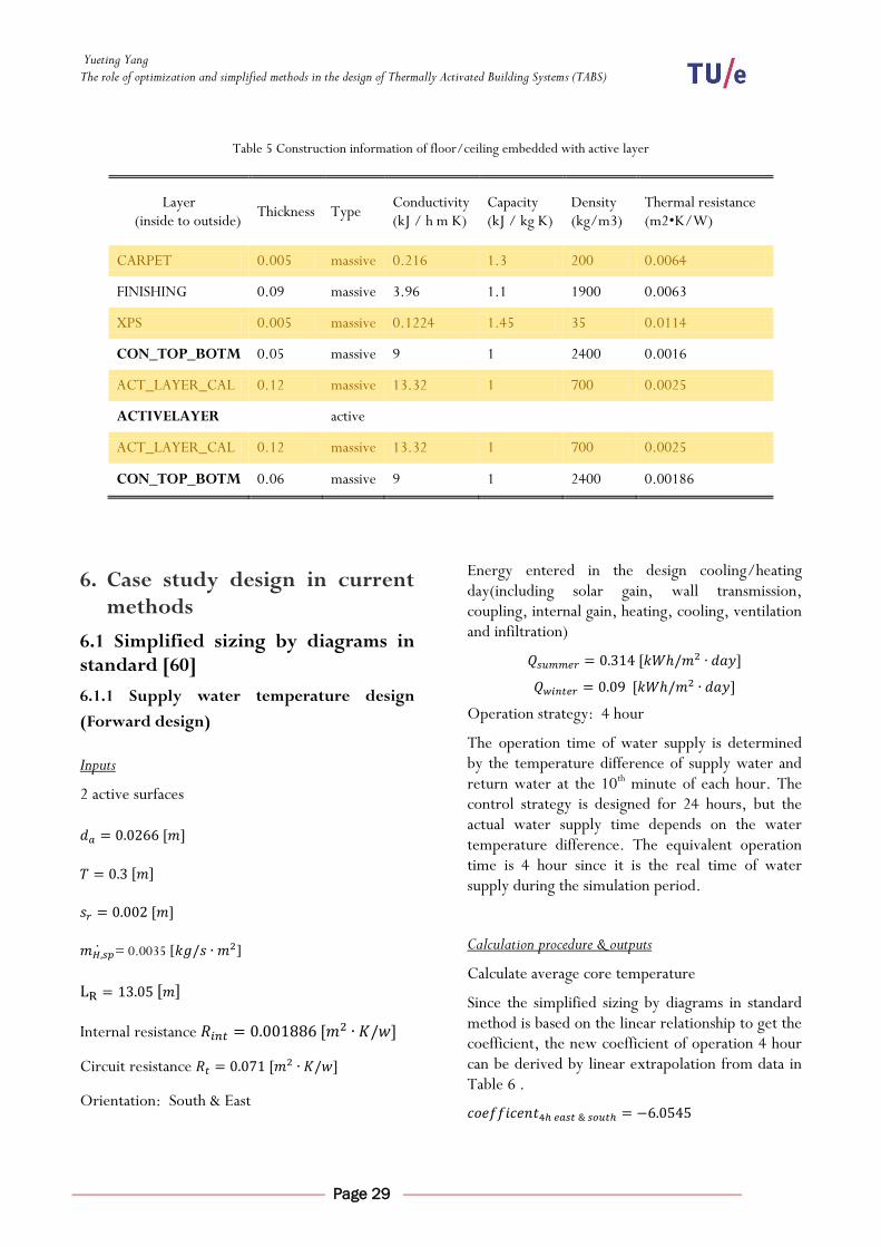
According to the building components information
(Table 5) of the ceiling/floor embedded with active
layer, the thermal resistance of the whole
construction is shown in Figure 35.
Figure 35 Thermal resistance model of floor/ceiling construction
Yueting Yang The role of optimization and simplified methods in the design of Thermally Activated Building Systems (TABS)
Page 29
Table 5 Construction information of floor/ceiling embedded with active layer
Layer (inside to outside)
Thickness Type Conductivity (kJ / h m K)
Capacity (kJ / kg K)
Density (kg/m3)
Thermal resistance (m2•K/W)
CARPET 0.005 massive 0.216 1.3 200 0.0064
FINISHING 0.09 massive 3.96 1.1 1900 0.0063
XPS 0.005 massive 0.1224 1.45 35 0.0114
CON_TOP_BOTM 0.05 massive 9 1 2400 0.0016
ACT_LAYER_CAL 0.12 massive 13.32 1 700 0.0025
ACTIVELAYER
active
ACT_LAYER_CAL 0.12 massive 13.32 1 700 0.0025
CON_TOP_BOTM 0.06 massive 9 1 2400 0.00186
6. Case study design in current methods
6.1 Simplified sizing by diagrams in standard [60]
6.1.1 Supply water temperature design
(Forward design)
Inputs
2 active surfaces
= 0.0035 [ ]
Internal resistance
Circuit resistance
Orientation: South & East
Energy entered in the design cooling/heating day(including solar gain, wall transmission, coupling, internal gain, heating, cooling, ventilation and infiltration)
Operation strategy: 4 hour
The operation time of water supply is determined by the temperature difference of supply water and return water at the 10th minute of each hour. The control strategy is designed for 24 hours, but the actual water supply time depends on the water temperature difference. The equivalent operation time is 4 hour since it is the real time of water supply during the simulation period.
Calculation procedure & outputs
Calculate average core temperature
Since the simplified sizing by diagrams in standard method is based on the linear relationship to get the coefficient, the new coefficient of operation 4 hour can be derived by linear extrapolation from data in Table 6 .
Yueting Yang The role of optimization and simplified methods in the design of Thermally Activated Building Systems (TABS)
Page 30
Table 6 Coefficient for average temperature calculation of the slab
Calculate the supply temperature for removing
cooling energy or supplying heating
energy
6.1.2 Dimension design (Reverse design)
Inputs
In reverse design, the supply water temperature come from the average value during simulation time in the reference design.
Internal resistance
Orientation: South & East
Energy entered in the design cooling/heating day(including solar gain, wall transmission, coupling, internal gain, heating, cooling, ventilation and infiltration)
Operation strategy: 4 hour
Calculation procedure & outputs
Calculate average core temperature
Calculate the circuit thermal resistance
Calculate the pipe dimension and specific mass flow rate
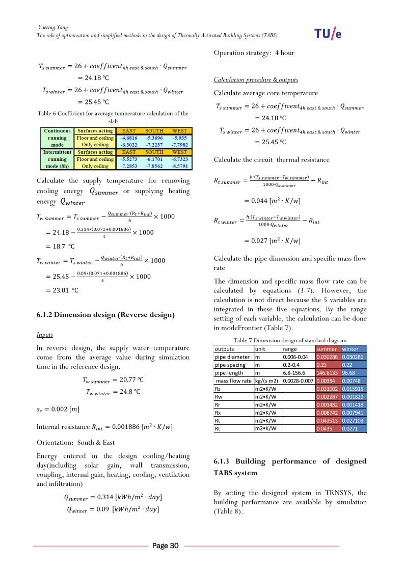
The dimension and specific mass flow rate can be calculated by equations (3-7). However, the calculation is not direct because the 5 variables are integrated in these five equations. By the range setting of each variable, the calculation can be done in modeFrontier (Table 7).
Table 7 Dimension design of standard diagram
6.1.3 Building performance of designed
TABS system
By setting the designed system in TRNSYS, the building performance are available by simulation (Table 8).
outputs unit range summer winter
pipe diameter m 0.006-0.04 0.030286 0.030286
pipe spacing m 0.2-0.4 0.23 0.22
pipe length m 6.8-156.6 146.6133 96.68
mass flow rate kg/(s m2) 0.0028-0.007 0.00384 0.00748
Rz m2•K/W 0.031002 0.015915
Rw m2•K/W 0.002287 0.001829
Rr m2•K/W 0.001482 0.001418
Rx m2•K/W 0.008742 0.007941
Rt m2•K/W 0.043513 0.027103
Rt m2•K/W 0.0435 0.0271

Yueting Yang The role of optimization and simplified methods in the design of Thermally Activated Building Systems (TABS)
Page 31
Table 8 Building performance from standard diagram design
6.2 Straightforward unknown but bounded method (SUB) [65]
6.2.1 Supply water temperature design
(Forward design)
Inputs
= 0.0035 [ ]
Internal resistance
Circuit resistance
Resistance of façade
According to the building components information
(Table 9) of external wall, the thermal resistance of
façade is
Outdoor average temperature
Room heating/cooling set-point
Energy entered in the design cooling/heating day(including solar gain, wall transmission, coupling, internal gain, heating, cooling, ventilation and infiltration)
Calculation procedure & outputs
Supply water temperature
For heating
( )
For cooling
( )
6.2.2 Dimension design (Reverse design)
Inputs
Internal resistance
Resistance of façade
Outdoor average temperature
Room heating/cooling set-point
Energy entered in the design cooling/heating day(including solar gain, wall transmission, coupling, internal gain, heating, cooling, ventilation and infiltration)
Supply water temperature
In reverse design, the supply water temperature come from the average value during simulation time in the reference design.
For heating
For cooling
summer 0.625 30
winter 0.634 0.33
summer 0.394 0
winter 0.771 0.067
Supply water
design
Dimension
design
weekly supply
energy (kJ/m2)
weekly uncomfortable
hours (hr)
Design
method

Yueting Yang The role of optimization and simplified methods in the design of Thermally Activated Building Systems (TABS)
Page 32
Table 9 Construction information of the facade
Layer (inside to outside) Thickness
(m) Type
Conductivity (kJ / h m K)
Capacity (kJ / kg K)
Density (kg/m3)
Thermal resistance (m2•K/W)
1GYPSONBOARD 0.013 massive 0.9 0.84 950 0.004012346
1CAVITY50 0.05 massive 1 1 1.2 0.013888889
1OSB 0.012 massive 0.468 1.3 650 0.007122507
1CELLULOSEINSULATION 0.184 massive 0.18 1.3 50 0.283950617
1WOODFIBERBOARD 0.018 massive 0.198 2.1 260 0.025252525
1CAVITY65 0.065 massive 1.3 1 1.2 0.013888889
1EXTERNALBRICKWORK 0.115 massive 4.86 0.84 1700 0.006572931
Calculation procedure & outputs Circuit resistance
The circuit thermal resistance is different in different seasons, which is not practical. For every dimension design, the calculated value is out of the range (Table 10). So the straightforward unknown but bounded method (SUB) cannot be used in the reverse way.
Table 10 Dimension design of straightforward unknown but bounded method (SUB)
range summer winter
Circuit resistance
( )
0.449 8.321
pipe diameter (m) 0.006-0.04 0.877 25.53
pipe spacing (m) 0.2-0.4 2.532 31.43
pipe length (m) 6.8-156.6 0.384 0.0117
mass flow rate
( ) 0.0028-0.007
0.00039 0.0000183
6.2.3 Building performance of designed
TABS system
By setting the designed system in TRNSYS, the building performance are available by simulation (Table 11).
Table 11 Building performance from straightforward unknown but bounded method (SUB)
6.3 Rehva guidebook [53]
The Rehva guidebook uses several supposed cases (Figure 38) to make diagrams for TABS design. Based on the dimension and supply water design in reference case, the Rehva guidebook can only be used in supply water temperature design (forward design).
6.3.1 Supply water temperature design
(Forward design)
Inputs
= 0.0035 [ ]
summer 0.3007 49.43
winter 0.0714 0
summer / /
winter / /
Dimension
design
Design methodweekly supply
energy (kJ/m2)
weekly uncomfortable
hours (hr)
Supply water
design

Yueting Yang The role of optimization and simplified methods in the design of Thermally Activated Building Systems (TABS)
Page 33
Figure 36 Heat exchange as the function of water temperature and floor covering (pipe spacing T= 150mm)
Figure 37 Heat exchange as the function of water temperature and floor covering (pipe spacing T= 300mm)

Yueting Yang The role of optimization and simplified methods in the design of Thermally Activated Building Systems (TABS)
Page 34
Heat exchange rate 37 [ ]
Floor covering resistance 0.0064
Figure 38 Sketches of calculated cases for capacity diagrams (thickness of structure layers, position of pipes)
Calculation procedure & outputs Pipe spacing
or
According to Figure 36 & Figure 37, the medium differential temperature can be decided.
For winter
For summer
For winter
For summer
Supply water temperature
According to the definition of the medium differential temperature (Equation 1), the supply water temperature is related to return water temperature and indoor operative temperature. The determination of supply water temperature has to be acquired by simulation in TRNSYS
(Equation 1)
For winter (no appropriate value)
For summer
For winter
For summer
6.3.2 Building performance of designed
TABS system
By setting the designed system in TRNSYS, the
building performance are available by simulation
(Table 12)
Table 12 Building performance from Rehva guidebook design method
6.4 Design manual from manufacture in USA [49]
There is only design for winter in this manual.
6.4.1 Supply water temperature design
(Forward design)
Inputs
Heat output ⁄
Indoor design temperature
Floor covering resistance The floor covering is carpet and the thermal resistance is 0.0064 in model. But in consideration of safety factor, the resistance is supposed to be 1 , which is decided by thickness of carpet.
range winter
pipe diameter (m) 0.006-0.04 0.017 0.017 0.017
pipe spacing (m) 0.2-0.4 0.15 0.3 0.3
pipe length (m) 6.8-156.6 13.05 13.05 13.05
0.0035
Circuit resistance
(m2K/W)0.05294 0.07137
mass flow rate
(kg/(s m2))0.0028-0.007 0.0035 0.0035
weekly supply energy
(kJ/m2)weekly uncomfortable
hours (hr)
1.64 0.97 1.79
0.37 22.70
summer
0.0714

Yueting Yang The role of optimization and simplified methods in the design of Thermally Activated Building Systems (TABS)
Page 35
Figure 39 Output chart of manual from manufacture in USA
Calculation procedure & outputs Floor surface temperature
According to Figure 39, heat output and indoor design temperature decide the floor surface temperature . The floor covering resistance is 1 , the supply water
temperature is .
Dimension design
Table 13 Pipe dimension and heat output chart
The pipe dimension can be decided by heat output (Table 13). The corresponding tube size of heat output can be 3/8'', 1/2'' and 3/4 ''. According to the system design guideline, the recommended pipe dimension for this residential building is 3/8''
Pipe diameter 0.01 [m]
Pipe spacing 0.23 [m]
The recommended length can be get by Table 14.
Table 14 Recommended tube length from manufacture in USA
Table 15 System design guideline from manufacture in USA
Number of circuit
=total pipe length/recommended pipe length

Yueting Yang The role of optimization and simplified methods in the design of Thermally Activated Building Systems (TABS)
Page 36
pipe length=total pipe length/number of circuit
=188.5/4=47.125 [m]
Mass flow rate
⁄
Pressure drop
The calculated supply water temperature is .
However, the minimal supply water temperature in
chart (Table 16 & Table 17) is . Supposed
the supply water temperature and head loss is linear
relationship , the pressure drop can be decided.
6.4.2 Dimension design (Reverse design)
Inputs
Supply water temperature (from reference case)
Floor covering resistance 1
Indoor design temperature
Calculation procedure & outputs Floor surface temperature
According to Figure 39, heat output and indoor design temperature decide the heat output
⁄ .
Dimension design
The pipe dimension can be decided by heat output (Table 13). The corresponding tube size of heat output can be 3/8'', 1/2'' and 3/4 ''. Compared with the forward design, the heat output is lower. So according to the system design guideline, the recommended pipe dimension is 1/2''
Pipe diameter 0.013 [m]
Pipe spacing 0.3 [m]
The recommended length can be get by Table 14.
Number of circuit
=total pipe length/recommended pipe length
pipe length=total pipe length/number of circuit
=143.6/2=71.8 [m]
Mass flow rate
⁄
Pressure drop
The calculated supply water temperature is
. However, the minimal supply water
temperature in chart (Table 16 & Table 17) is
. Supposed the supply water temperature
and head loss is linear relationship , the pressure
drop can be decided.

Yueting Yang The role of optimization and simplified methods in the design of Thermally Activated Building Systems (TABS)
Page 37
Table 16 Head loss when supply water temperature at 100

Yueting Yang The role of optimization and simplified methods in the design of Thermally Activated Building Systems (TABS)
Page 38
Table 17 Head loss when supply water temperature at 120

Yueting Yang The role of optimization and simplified methods in the design of Thermally Activated Building Systems (TABS)
Page 39
6.4.3 Building performance of designed
TABS system
By setting the designed system in TRNSYS, the building performance are available by simulation (Table 18).
Table 18 Building performance from TABS design manual of manufacture in USA
6.5 Design manual from manufacture in Canada [55]
There is only design for winter in this manual.
6.5.1 Supply water temperature and
dimension design (Forward design)
Inputs
Heat output ⁄
Area 6.76m * 6.95m =
Temperature difference of supply and return water
Floor covering resistance The floor covering is carpet and the thermal resistance is 0.0064 in model. But in consideration of safety factor, the resistance is supposed to be 1 , which is decided by thickness of carpet.
Calculation procedure & outputs Pressure drop
=2.22 GPM
According to the relationship of flow rate and heat output (Figure 40), there are several choices for dimension design (Table 19).
Table 19 Distance on center and flow rate
Distance on center(inch) Flow rate (GPM)
6 1.1
9 1.6
12 2.2
To meet the requirement of pressure drop, the
distance on center has to be 12 inch.
Supply water temperature
By heat loss and resistance of floor covering, the
supply water temperature can be decided (Figure
41).
Dimension design
The pipe dimension and pressure drop has to fit the
following relationship (Table 20). The requirement
of this system is 2.2, the possible dimension designs
are listed in Table 21.
Table 20 Pipe dimension and pressure drop relationship
Table 21 Possible dimension designs at total pressure drop 2.2 GPM
range
pipe diameter (m) 0.006-0.04 0.01 0.013
pipe spacing (m) 0.2-0.4 0.23 0.3
pipe length (m) 6.8-156.6 47.125 71.8
weekly uncomfortable
hours (hr)0.17 4.37
Supply water
design
Dimension
design
mass flow rate
(kg/(s m2))
0.0028-
0.0070.0035 0.0021
weekly supply energy
(kJ/m2)0.8 1.34
winter
Circuit resistance
(m2K/W)0.061 0.092
1 2.2 3 1'' 506 600-750
3 1'' 253 600-750
1.7 3/4'' 253 500-600
1.3 5/8'' 253 325-500
3 1'' 169 600-750
1.7 3/4'' 169 500-600
1.3 5/8'' 169 325-500
1 1/2'' 169 250-325
Tube
size
Loop length
(ft)
Recommended
loop length (ft)
2
3 0.7
1.1
Flow rate
(GPM)
Number
of circuit
Max flow
rate

Yueting Yang The role of optimization and simplified methods in the design of Thermally Activated Building Systems (TABS)
Page 40
Figure 40 Flow rate and heat output chart at 10 supply/return temperature differential
Figure 41 Water supply temperature for 12 inch on center

Yueting Yang The role of optimization and simplified methods in the design of Thermally Activated Building Systems (TABS)
Page 41
All the designed pipe length are not in the range of
recommended loop length. So there are two
possible designs which are most close to the range
of recommended loop length: 3/4''& 5/8''.
6.5.2 Building performance of designed
TABS system
By setting the designed system in TRNSYS, the
building performance are available by simulation
(Table 22).
Table 22 Building performance from TABS design manual of manufacture in Canada
7. Single pipe dimension optimization
7.1 Simulation and modeling
TRNSYS model
The simulation in MODEFRONTIER is integrated with the basic ‘only building’ TRNSYS model. The indoor environment of building is only controlled by the TABS system without other heating or cooling equipment. The supply water temperature of TABS is controlled by the ambient temperature and supply water flow rate is controlled by the temperature difference of supply and return water(TABS outlet) temperature at 10th minute of each hour. The air handling unit(AHU) is responsible for the ventilation and the boiler works as a supplement in heating mode.
TRNSYS simulation time
4837-5004hr, a typical summer week in July
Input variable
According the thermal resistance model, there are pipe sizing related parameters: pipe diameter, pipe distance, deepness of embedded pipe and specific mass flow rate.
-pipe diameter of active layer, which ranges from 0.006m to 0.04m with a step of 0.0005m
-pipe spacing between pipe centers, which ranges from 0.2m to 0.4m with a step of 0.01m
--pipe deepness, which ranges from 0.09m to 0.13m inside original active layer(from the pipe position to the outside covering) with a step of 0.01m
Optimization Method
Design of experiment(DOE)—Uniform Latin Hypercube, number of designs: 200
Scheduler—Multi objective genetic algorithm(MOGA-II), generations: 10
Objectives
Minimizing E_tot:
E_tot indicates the thermal demand of building, which includes both heating and cooling capacity of TABS system.
Minimizing Overheating:
Overheating is the weekly overheating hours which generates when the average building temperature is larger than 26 ˚C.
7.2 Thermal demand and pipe dimension
According to Figure 42, Figure 43 & Figure 44, the thermal demand increases when pipe diameter or pipe deepness increases and decreases when pipe spacing increases. Thermal demand is the integration result of thermal capacity of TABS over the simulation time.
a. The thermal capacity of TABS system is
determined by both temperature difference of
supply and return water, and the water mass
flow rate (Equation 8).
pipe diameter (m) 0.006-0.04 0.022 0.019
pipe spacing (m) 0.2-0.4 0.3 0.3
pipe length (m) 6.8-156.6 28 28
weekly supply energy
(kJ/m2)5.04 5.13
weekly uncomfortable
hours (hr)49.9 49.93
Circuit resistance
(m2K/W)0.042 0.042
mass flow rate
(kg/(s m2))0.0028-0.007 0.008 0.008
winter
3/4'' 5/8''range

Yueting Yang The role of optimization and simplified methods in the design of Thermally Activated Building Systems (TABS)
Page 42
b. According to the simulation data (Figure 45 &
Figure 47), the temperature difference is not
large, so the determinant factor is water mass
flow rate, which increases with the pipe
diameter growth (Figure 46 & Figure 48).
( )
(Equation 8)
Return flow rate
( )
(Equation 9)
c. And the specific mass flow rate is determined
by the temperature difference at 10 minute of
supply and return water as shown in (Equation
9), which is described in the TRNSYS
model(Every hour, water circulates for the first 10
minutes. Then, calculate temperature difference of
supply and return water at 10th minute, If
temperature difference is higher than 2°C, the water
will circulate for the next 50 minutes; If temperature
difference is lower than 2°C, the water pump stops for
the next 50 minutes).
7.2.1 Pipe diameter optimization and
thermal supply
In this sense, the probability of temperature difference at the first 10th min of each hour is larger than 2°C increases with the growth of pipe diameter, as shown in Figure 49. The temperature difference of return water and supply water at 10th of ceiling in zone1 is plotted, and larger the pipe diameter, more dots are over the boundary of 2˚C. All the points indicate either pipe diameter has more water supply opportunity than the other one. So the more dots over the 2˚C boundary, the more possibility of water supply.
This is because the heat transfer determinant depends on the specific situation. With smaller pipe diameter, the velocity in pipe is faster and the contact area is smaller. In this sense, heat transfer is
less sufficient because of fast velocity so the temperature difference of supply and return water is not so large. While in the case of larger pipe diameter, the velocity in pipe is slower and more contact area is available. It takes more time for heat transfer and the temperature difference is larger, but the average temperature difference is smaller because of more sufficient heat transfer.
Figure 42 Pipe diameter optimization and weekly thermal supply
Figure 43 Pipe spacing optimization and weekly thermal supply
Figure 44 Pipe deepness optimization and weekly thermal supply

Yueting Yang The role of optimization and simplified methods in the design of Thermally Activated Building Systems (TABS)
Page 43
Figure 45 Temperature and mass flow rate in TABS outlet (pipe diameter)
Figure 46 Mass flow rate and pipe diameter
Figure 47 Temperature and mass flow rate in TABS outlet (pipe spacing)
Figure 48 Mass flow rate and pipe spacing
7.2.2 Pipe spacing optimization and thermal
supply
When there is a larger pipe spacing, the probability of temperature difference at first 10th min of each hour is decreasing (Figure 50). The temperature difference of return water and supply water at 10th of ceiling in zone1 is plotted, and smaller the pipe spacing, more dots are over the boundary of 2˚C. All the points indicate the water supply schemes of two pipe spacing systems are different from each other. So the more dots over the 2˚C boundary, the more possibility of water supply. And the smaller pipe spacing has more water supply opportunity than the larger ones. This is because the decreasing pipe spacing results in longer loop length, according to equation 2. Then the more heat will be delivered to the building and more thermal comfort will be achieved.
7.2.3 Pipe deepness optimization and
thermal supply
There is not much difference in thermal supply for both ceiling and floor cases when pipe deepness changes. This is because the determinant outlet water temperature and mass flow rate do not change much as well. The changeable range of deepness is quite narrow because of the characteristics of active layer. According to the TRNSYS manual, there are several rules for active layer design (Figure 52).
a. For entering the layers of the floor heating
system start with a thickness of the later
adjacent to the active later with a
thickness≥0.3*pipe spacing.
b. Define an active layer. Automatically, a new
layer with the same properties of the layer
above the active layer is added below.
c. Enter an insulation layer with a resistance of at
least 0.825 .
d. The thickness of the layer between the active layer and the insulation layer≥1/2* outside pipe diameter.

Yueting Yang The role of optimization and simplified methods in the design of Thermally Activated Building Systems (TABS)
Page 44
Figure 49 Temperature difference of supply and return water at 10th minute of ceiling in zone1 (pipe diameter)
Figure 51 Temperature difference of supply and return water at 10th minute of ceiling in zone1 (pipe deepness)
Figure 1 Temperature difference of supply and return water at 10th minute of ceiling in zone1 (pipe spacing)

Yueting Yang The role of optimization and simplified methods in the design of Thermally Activated Building Systems (TABS)
Page 45
In this case, the possible range of pipe deepness is quite limited, which indicates the pipe deepness is not a determinant factor for optimization (Figure 51).
Figure 52 Scheme of active layer in TRNSYS
7.3 Overheating hours and pipe dimension
7.3.1 Pipe diameter optimization and
overheating hours
As shown in Figure 53, weekly overheating hours decreases when pipe diameter increases. This could be explained by the declining return water temperature in pipes with the increase of pipe diameter, shown in Figure 54. The temperature of supply water is controlled by outdoor ambient temperature. The temperature difference is decreasing, which indicates TABS system absorbing more heat. In this case, a more comfortable indoor environment and less overheating hours would be achieved.
Figure 53 Pipe diameter optimization with weekly overheating hours
Figure 54 Pipe water temperature, indoor air temperature and pipe diameter
7.3.2 Pipe spacing optimization and
overheating hours
As indicated in Figure 55, more overheating hours results from larger pipe spacing. This is because the return water temperature grows larger in larger spacing system (Figure 56). The larger pipe spacing, the smaller output is. Then the TABS system absorbs less heat and results in higher indoor temperature in the case of larger pipe spacing.
Figure 55 Pipe spacing optimization and weekly overheating hours
Figure 56 Pipe water temperature, indoor air temperature and pipe spacing

Yueting Yang The role of optimization and simplified methods in the design of Thermally Activated Building Systems (TABS)
Page 46
7.3.3 Pipe deepness optimization and
overheating hours
Figure 57 Pipe deepness optimization and overheating hours
There is not much difference in overheating hours for both ceiling and floor cases when pipe deepness changes (Figure 57).
7.4 Pareto front in single dimension optimization
Considering the two conflicting objectives: low thermal demand and high thermal comfort, the multi-objective genetic algorithm is applied to solve the problem. To compare with energy and comfort standard, the annual results of some points are also indicated. Unfilled dots are the dominated solutions and the filled ones are a set of optimal trade-offs(all objectives are equally important), which is called the non-dominated solution or PARETO FRONT. The Pareto front of pipe diameter and pipe spacing optimization are shown in Figure 58 & Figure 59.
Since there are restrictions on both objectives, the selected solutions can be determined by the specific purpose of the TABS system designers.
a. According to Energy Benchmarks Codes &
Standards, the annual thermal demand for low
energy consumption office building is
40kWh/m2•yr and 15kWh/m2•yr for passive
office buildings. Compared with this code, the
designers for TABS system could get an
appropriate range of pipe diameter for specific
building types. For example, there are some
disadvantages for a passive house, such as
system running noise and high overheating hour
risk. In this case, the annual thermal demand
should be more than 15kWh/m2•yr to avoid
the drawbacks of passive house.
b. Given the standard from the Government
Buildings Agency and the Government
Occupational Health Agency in the
Netherlands, a good thermal indoor climate had
to comply with the limitations:
25˚C may not be exceeded during
maximally 100 hours a year;
28˚C may not be exceeded during
maximally 10-20 hours a year;
In the case of TRNSYS model, the overheating set point is 26˚C, and it is obvious that all the annual overheating hours exceed far higher than the standard limit. The whole building is suffered from severe overheating problem. As for the energy demand, this building is in a quite energy-saving way.

Yueting Yang The role of optimization and simplified methods in the design of Thermally Activated Building Systems (TABS)
Page 47
Figure 58 Energy demand and thermal comfort of a typical summer week in July with PARETO FRONT (pipe diameter)
Figure 59 Energy demand and thermal comfort of a typical summer week in July with PARETO FRONT (pipe spacing)
700 800 900 1000 1100 1200 1300 140020
21
22
23
24
25
26
27
28
Weekly thermal demand from TABS[kJ/m2.week]
Weekly
overh
eating h
ours
[hr]
Energy demand and thermal comfort of a typical summer week in July
3mm
10mm
17mm
24mm
31mm
38mm
45mm
weekly simulation result
pareto front
ORIGINAL PIPE DIAMETER 0.0266m
Annual overheating hours 785hr
Annual thermal demand 22.51kWh/m2
PIPE DIAMETER 0.006m
Annual overheating hours906hr
Annual thermal demand18.42kWh/m2
PIPE DIAMETER 0.04m
Annual overheating hours 756hr
Annual thermal demand23.35kWh/m2
950 1000 1050 1100 1150 1200 1250 1300 1350 1400 145018
19
20
21
22
23
24
Weekly thermal demand from TABS[kJ/m2.week]
Weekly
overh
eating h
ours
[hr]
Energy demand and thermal comfort of a typical summer week in July
20cm
22cm
24cm
26cm
28cm
30cm
32cm
34cm
36cm
38cm
40cm
weekly simulation result
pareto front
Pipe spacing 20cm
Annual overheating hours 713hr
Annual thermal demand 24.35kWh/m2
Pipe spacing 40cm
Annual overheating hours 821.6hr
Annual thermal demand 21.03kWh/m2
ORIGINAL pipe spacing 30cm
Annual overheating hours 785hr
Annual thermal demand 22.51kWh/m2

![A SIMPLIFIED DOLPHIN ECHOLOCATION OPTIMIZATION …ijoce.iust.ac.ir/article-1-183-en.pdf · Optimization algorithm (CBO) [12] and Enhanced colliding bodies optimization [13]. Recently,](https://img.dokumen.tips/doc/110x75/5edec40dad6a402d666a1d84/a-simplified-dolphin-echolocation-optimization-ijoceiustacirarticle-1-183-enpdf.jpg)