The Robustness of CAPM-A Computational Approach�

P. Jean-Jacques Heringsy

Department of Economics

University of Maastricht

Felix Kublerz

Department of Economics

Stanford University

January 21, 2000

Abstract

In this paper we argue that in realistically calibrated two period general equilib-

rium models with incomplete markets CAPM-pricing provides a good benchmark for

equilibrium prices even when agents are not mean-variance optimizers and returns

are not normally distributed. We numerically approximate equilibria for a variety

of di�erent speci�cations for preferences, endowments and dividends and compare

the equilibrium prices and portfolio-holdings to the predictions of CAPM. While we

show that CAPM cannot hold exactly for the chosen speci�cation, it turns out that

pricing-errors are extremely small. Furthermore, two-fund separation holds approxi-

mately.

JEL codes: C61, C62, C63, C68, D52, D58, G11, G12.

Keywords: asset pricing, general equilibrium, incomplete markets, computational

methods.

�The research of Jean-Jacques Herings has been made possible by a fellowship of the Royal Netherlands

Academy of Arts and Sciences and a grant of the Netherlands Organization for Scienti�c Research (NWO).

While this paper was being written this author enjoyed the generous hospitality of the Cowles Foundation

for Research in Economics at Yale University, of CORE at Universit�e Catholique de Louvain, and of

CentER at Tilburg University. Felix Kubler gratefully acknowledges the �nancial support of the Cowles

Foundation in the form of an Anderson dissertation fellowship.yP.J.J. Herings, Department of Economics, University of Maastricht, P.O. Box 616, 6200 MD Maas-

tricht, The Netherlands. E-mail: P.Herings@algec.unimaas.nlzF. Kubler, Department of Economics, Stanford University, Stanford, California 94305-6072, USA.

1

1 Introduction

The capital asset pricing model (CAPM) of Sharpe (1964) and Lintner (1965) pre-

dicts that equilibrium returns of assets are a linear function of their market � (the slope

in the regression of a security's return on the market's return). This intuitively appealing

result has long shaped the way practitioners think about average returns and risk. While

the model fares poorly in explaining observed cross-sectional stock returns (see for exam-

ple Fama and French (1992)) it remains one of the central building blocks in �nancial

economics.

One of the reasons for this is that the CAPM provides a good theoretical starting point

for the examination of asset prices. Geanakoplos and Shubik (1990) show that CAPM

can be viewed as a special case of the general equilibrium model with incomplete asset

markets (the GEI-model). Oh (1996), Willen (1997) and others have shown that the

central conclusions of CAPM, the pricing formula, holds true under completely general

dividends and endowments as long as all agents have mean-variance utility functions.

However, without mean-variance preferences one has to make very strong assumptions

on the distribution of asset pay-o�s in order to derive the conclusions of CAPM1. Berk

(1997) shows that joint restrictions on utility functions and asset returns cannot lead to

more realistic assumptions. He shows that if one assumes that agents have von-Neumann-

Morgenstern utility functions, quadratic utility is necessary for the CAPM-pricing formula

to hold. Since quadratic utility is an unattractive assumption, it is an important question

whether CAPM-pricing provides a benchmark for the cross section of security prices in a

model with more general preferences, endowments and asset returns. Empirical contradic-

tions of CAPM might be explained by the fact that some agents are not mean-variance

optimizers and that many securities have returns that are far from elliptical.

In this paper we show that independently of mean-variance preferences or normal re-

turns, the CAPM pricing formula often provides a very good prediction for actual equi-

librium returns. It is clear, of course, that it is always possible to construct economies

where equilibrium asset prices are arbitrarily far from those predicted by CAPM. We do

not provide a theoretical explanation for the documented phenomenon but instead com-

pute hundreds of examples which illustrate it (see Judd (1997) for a general discussion

which favors this approach to economic theory) - we approximate equilibria numerically

(using the algorithm developed in Herings and Kubler (2000)) and compare the prices and

portfolio-holdings predicted by CAPM to the actual equilibrium prices and equilibrium

portfolio-holdings. In all cases we consider, CAPM pricing is an excellent benchmark for

the equilibrium prices. These results are robust with respect to variations in preferences,

endowments and dividends.

In order to show that the CAPM pricing formula provides a good approximation to

asset returns in realistically calibrated models, one �rst has to clarify what one means

by 'realistically calibrated'. We follow the macroeconomic literature and we choose �rst

1Ross (1978) provides a complete characterization of the class of separating distribution

2

and second moments of endowments and dividends to roughly match annual US data

and preferences to exhibit relative risk aversion below 10 and nondecreasing absolute risk

aversion (see e.g. Mehra and Prescott (1985))2.

More importantly one has to argue that the computed examples are not sensitive to

the exact speci�cation of the model but that they re ect some general property of asset

prices. We assume that there are three agents and 32; 768 states of nature and we examine

the robustness of CAPM with respect to 600 di�erent speci�cations of preferences and

endowments: We �rst assume that endowments and dividends are log-normally distributed

and consider the following 3 speci�cations for preferences.

� All three agents have constant absolute risk aversion (CARA) utility functions.

� All agents' utility functions exhibit constant relative risk aversion (CRRA).

� Agents' utility-functions exhibit loss aversion as in Benartzi and Thaler (1995).

For each case we randomly generate 100 economies which di�er with respect to agents'

(heterogeneous) degrees of risk aversion.

In the next three cases we �x preferences and vary distributions of dividends and

endowments. We assume that all agents have CRRA utility functions and consider the

following distributions for assets and endowments.

� Endowments and dividends are drawn from a uniform distribution, We randomly

generate 100 economies with di�er with respect to the support of the uniform distri-

butions.

� Endowments and dividends are determined by two factors and an idiosyncratic shock

each of which are drawn from a log-normal distribution. We randomly generate 100

economies with di�er with respect to the factor-loads.

� Endowments and dividends are drawn from a log-normal distribution and there is an

option on one of the stocks. We randomly generate 100 economies which di�er with

respect to the strike-price of the option.

For all 600 economies under consideration we compare the computed return on indi-

vidual stocks to the return predicted by the CAPM-pricing formula. We �nd that in all

600 cases the average mean squared pricing errors (for returns) across stocks lie below 0.04

percent. The average error across all simulations is in the order of magnitude of 0.005

percent. In addition to predicting asset returns, the CAPM also predicts that all agents'

equilibrium portfolio-holdings will consist of the riskless bond and a mutual fund of risky

assets. It is possible that CAPM-pricing is very accurate, but two-fund separation does not

2Note that just as in Mehra and Prescott this calibration is very unrealistic with respect to the market

risk-premium. This fact might give a �rst indication of why CAPM-pricing does so well in our framework.

3

apply. Nevertheless, in the computed examples two-fund separation holds almost exactly

in the equilibria we compute.

The paper is organized as follows. In Section 2 we give a short introduction to the model

and collect several general results on CAPM in a general equilibrium setting. Section 3

gives an example of a realistically calibrated economy with non-elliptical returns and CRRA

preferences for which CAPM-pricing provides an almost perfect prediction. In Sections 4

and 5 we examine the robustness of this phenomenon. In Section 4 we vary the parameters

of risk aversion for the CRRA case, we consider CARA utility functions, and we examine

utility functions displaying loss aversion. In Section 5 we �x preferences to exhibit constant

relative risk aversion and we examine the robustness of CAPM with respect to dividend-

distributions. In Section 6 we speculate about possible explanations and conclude the

paper.

2 The Two-Period Finance Economy

The �nance version of the GEI-model describes an economy over two periods of time,

t = 0; 1; with uncertainty over the state of nature resolving in period t = 1. We describe the

model, introduce the necessary notation and discuss the CAPM. For a thorough description

of the GEI-model see for example Magill and Quinzii (1996).

2.1 The Model

There are S + 1 states in the economy; at time t = 0 the economy is in state s = 0; at

time t = 1 one state of nature s out of S possible states of nature realizes. In each state

s = 0; : : : ; S; there is a single nondurable consumption good.

There are H agents, indexed by h = 1; : : : ; H; that participate in the economy. Each

agent h is characterized by initial endowments (the initial income stream) eh = (eh0 ; eh1 ; : : : ; e

hS)

> 2int(Xh)3 and his preferences over consumption bundles (income streams available for con-

sumption) ch = (ch0 ; ch1 ; : : : ; c

hS)

> 2 Xh. Here Xh is a closed subset of IRS+1 that satis�es

fxhg+IRS+1+ � Xh for all xh 2 Xh: In most applicationsXh will be equal to IRS+1

+ or IRS+1:

To distinguish between �rst-period consumption and the random second period consump-

tion, we de�ne ex = (x1; : : : ; xS)> for any vector x = (x0; x1; : : : ; xS)

>. Aggregate endow-

ments (aggregate incomes) are e =PH

h=1 eh: Each agents' preferences are represented by a

utility function uh : Xh ! IR satisfying standard assumptions; uh is strictly quasi-concave

and continuous. Moreover, the set Xh(eh) = fxh 2 Xh j uh(xh) � uh(eh)g is assumed

to be bounded from below, a property automatically satis�ed when Xh is bounded from

below. In the applications of Sections 3 � 5 we consider economies where all agents have

separable utility functions across date-events with identical probabilities, i.e. there exist

3int(Xh) denotes the interior of Xh:

4

probabilities �1; : : : ; �S > 0;PS

s=1 �s = 1, such that

uh(ch) = vh0 (ch0) + �h

SXs=1

�svhs (c

hs );

where �h > 0 is the discount factor, Xh =QS

s=0Xhs ; where Xh

s is a subset of IR; and

vhs : Xhs ! IR is assumed to be strictly increasing and strictly concave. In this case it follows

from the properties of vhs that Xh(eh) is bounded from below. When the functions vhs are

independent of s; we say that agents have von Neumann-Morgenstern utility functions.

There are J assets. Asset j pays dividends at date t = 1 which we denote by dj 2 IRS:

The price of asset j at time t = 0 is qj. Without loss of generality we assume that the

assets are in zero net supply and we collect all assets' dividends in a pay-o� matrix

A = (d1; ::::; dJ) 2 IRS�J :

At time t = 0 agent h chooses a portfolio-holding �h 2 IRJ which uniquely de�nes the

agents' consumption by ech = eeh + A�h and ch0 = eh0 � �h � q. The net demand of agent h;ech � eeh; belongs to the marketed subspace hAi = fz 2 IRS j 9� 2 IRJ ; z = A�g:The exogenous parameters de�ning a �nance economy E = ((Xh; uh; eh)h=1;:::;H ;A)

are agents' consumption sets, utility functions and endowments, and the pay-o� matrix.

Without loss of generality, we assume throughout that there are no redundant assets,

rank(A) = J: If there are redundant assets, it follows from an arbitrage argument that

their price is uniquely determined by the price of the other assets. Markets are incomplete

when J < S. We de�ne asset prices to be arbitrage free if it is not possible to achieve a

positive income stream in all states by trading in the available assets. It is well known that

a price system q 2 IRJ precludes arbitrage if and only if there exists a state price vector

� 2 IRS++ such that q = �>A. We de�ne Q to be the set of arbitrage free asset prices.

Definition 2.1 (Competitive Equilibrium): A competitive equilibrium for an

economy E is a collection of portfolio-holdings �� = (�1�; : : : ; �H�) 2 IRHJ and asset prices

q� 2 IRJ that satisfy the following conditions:

(1) �h� 2 argmax�h2IRJ uh(ch) s:t: ch = eh +

�q�>

A

!�h and ch 2 Xh; h = 1; : : : ; H;

(2)PH

h=1 �h� = 0.

Under an additional assumption of strictly increasing utility functions, existence of an

equilibrium follows from the results of Geanakoplos and Polemarchakis (1986).

2.2 The Capital Asset Pricing Model

Sharpe (1964) and Lintner (1965) use the portfolio analysis developed by Tobin (1958)

and Markowitz (1959) to examine an equilibrium model of �nancial markets. Under the

5

assumption that all agents are mean-variance optimizers they derive a closed-form solution

for equilibrium returns, the so-called �-pricing formula. This formula relates the return of

a risky asset to the return of the market portfolio by the covariance of that asset with the

market. It is well known that the �-pricing formula can be derived in the �nance GEI-

model, see Geanakoplos and Shubik (1990). To �x notation and to give some intuition

for the computational results in Sections 3� 5; we summarize and slightly generalize the

�ndings in the literature - Geanakoplos and Shubik (1990), Magill and Quinzii (1996), Oh

(1996), and Willen (1997) - to cover the case with mean-variance preferences, non-marketed

endowments and a �nite state space in a world with incomplete markets.

We denote by 1n = (1; : : : ; 1)> 2 IRn the vector of all ones. The m-th unit vector of

appropriate dimension is denoted �m - the dimension of �m is always apparent from the

context. Throughout this subsection we assume that there exist objective probabilities �s;

s = 1; : : : ; S; over the possible states of nature in period 1: Moreover, asset 1 is a riskless

bond, d1 = 1S. For a random variable x 2 IRS; we de�ne its expected value E(x) =PSs=1 �sxs, for two random variables x; y 2 IRS; we de�ne the covariance as cov(x; y) =PSs=1 �sxsys � E(x)E(y): The variance of a random variable x 2 IRS is given by var(x) =

cov(x; x). Finally, we de�ne x �� y =PS

s=1 �sxsys for vectors x; y 2 IRS.

For any competitive equilibrium (��; q�); there exists a unique state price vector in the

marketed subspace ��A 2 hAi such that, for all assets j q�j = ��A �� dj: Using the de�nitionsof variance and covariance, this implies

q�j = E(��A)E(dj) + cov(��A; d

j): (1)

We de�ne the return of a portfolio � 2 IRJ with q� � � 6= 0 by r� =A�q���

and we denote the

return of the riskless bond by Rf = 1q�1

: With this we rewrite equation (1) as

q�j =1

RfE(dj) + cov(��A; d

j):

We de�ne the pricing portfolio as the unique portfolio ��A which solves A��A = ��A.

Notice that

q� � ��A = ��A �� A��A = ��A �� ��A > 0;

where ��A 6= 0 follows from E(��A) = q�1 > 0:

Since the return of the pricing portfolio satis�es r��A=

A��A

q����A

=��A

��A����A

we can rewrite

equation (1) as

E(r�)� Rf =cov(r�; r��

A)

var(r��A)

(E(r��A)� Rf): (2)

While equation (2) relates the prices of the risky assets and looks similar to the CAPM

pricing formula, this formula is rather useless if we have no further information on ��A. Note

that so far all formulas followed simply from the absence of arbitrage. It is well known that

under the assumption that one agent h's utility function is di�erentiable and that in an

6

equilibrium with individual consumption (ch�)h2H , agent h's utility maximization problem

has an interior solution, ��A can be characterized as

��A = projhAi

0@@ch1uh(ch�)=�s@ch

0

uh(ch�); : : : ;

@chSuh(ch�)=�s

@ch0

uh(ch�)

1A ;

where projhAi denotes the projection on hAi under the inner product �.One possibility to derive an interesting pricing formula is to assume that all preferences

just depend on the mean and the variance of consumption,

uh(ch) = wh(ch0 ;E(ech); var(ech));where wh is strictly increasing in ch0 and in the expected consumption and strictly decreasing

in the variance of consumption.

Agent h's �rst period endowments can be decomposed into a marketed part and a non-

marketed part, where the latter part lies orthogonal to the marketed subspace under the

inner product �: We write

eeh = eehM + eeh?and have by de�nition eeh? �� z = 0 for all z 2 hAi. This decomposition is uniquely deter-

mined. We de�ne the marketed endowments eeM =PH

h=1eehM and the market portfolio �M

as the unique portfolio satisfying

A�M = eeM:Note that it may happen that q� � �M = 0; even when ee� 0:4

To simplify matters, we �rst assume q� � �M 6= 0 and then argue that this assumption is

not necessary. Given a competitive equilibrium (��; q�); we de�ne �� for a portfolio � 2 IRJ

by

�� =cov(r�; r�M)

var(r�M):

Then we have the following result.

Theorem 2.3: Under the assumptions that all agents maximize mean-variance util-

ity functions with objective probabilities �; var(eeM) > 0, and there is a riskless bond, each

equilibrium (��; q�) of E with equilibrium consumption (c1�; : : : ; cH�) has the following prop-

erties.

1. The CAPM-pricing formula holds; when q� � �M 6= 0; then for each � 2 IRJ ;

E(r�)�Rf = ��(E(r�M)� Rf): (3)

4For a vector x 2 IRm we use the notation x � 0 if x 2 IRm+ ; x > 0 if x 2 IRm+ n f0g; and x � 0 if

x 2 IRm++:

7

2. Two-fund separation holds; for each agent h there exists (�h1 ; �

h2) 2 IR � IR+; wherePH

h=1 �h1 = 0 and

PHh=1 �

h2 = 1; such that

ech� � eeh? = �h11S + �h

2A�M:

3. The pricing vector satis�es ��A = �11S � �2eeM; with �1 > �2E(ee) and �2 strictly

positive.

Proof. We �rst show that a pseudo two-fund separation holds in the sense that the

agents' consumption bundles can be written as ech� = eeh?+ e�h11S+ e�h

2��A for some e�h

1 ; e�h2 2 IR.

De�ne

ech = eeh? + projh1S ;��Ai(ech�):

Suppose pseudo two-fund separation does not hold, so ech 6= ech�. Since ��A �� (ech�� ech) = 0;

it follows that the portfolios needed to consume ech� and ech are as expensive at date 0.

Moreover, eeh? �� (ech� � ech) = 0 and 1S �� (ech� � ech) = 0; so it follows that E(ech� � ech) = 0

and cov(ech� � ech; ech) = 0: Therefore, E(ech�) = E(ech) and var(ech�) > var(ech); giving a

contradiction to the optimality of ech� at prices q�: We obtain pseudo two-fund separation.

Since in equilibrium eeM =PH

h=1(ech� � eeh?), the two-fund separation property implies

that eeM 2 h1S; ��Ai. The assumption var(eeM) > 0 implies that eeM is not collinear to 1S

and it holds that ��A = �11S��2eeM for some numbers �1; �2: Two-fund separation follows

immediately, ech� � eeh? = �h11S + �h

2A�M for some numbers �h1 ; �

h2 :

Since eeM =PH

h=1 �h11S +

PHh=1 �

h2eeM and var(eeM) > 0; we have

PHh=1 �

h1 = 0 andPH

h=1 �h2 = 1: Consider a consumption bundle ch� that results from using the income that

is invested in the market portfolio to buy the riskless bond, so ech� = eeh? + �h11S + �h

2(��A ��

A�M=q�1)1S: The portfolios needed to consume ech� and ech� are as expensive since ��A �� (ech��ech�) = 0: Since var(ech�) � var(ech�) and uh(ch�) � uh(ch�); it holds that E(ech�) � E(ech�) =

�(�h2�2=q

�1)var(eeM) � 0; where we use that ��A��A�M = q�1E(eeM)��2var(eeM): The preceding

inequalities are strict inequalities when �h2 > 0; which is the case for at least one agent.

Then it follows that �2 > 0 and �h2 � 0; h = 1; : : : ; H: Since 0 < q�1 = E(��A) = �1 �

�2E(eeM); and 1S �� ee? = 0; so E(eeM) = E(ee); it holds that �1 > �2E(ee):The CAPM pricing formula is obtained by substituting ��A = �1�1��2�M in equation (2).

From

cov(r�; r��A)

var(r��A)

= � q� � ��A�2q� � �M

cov(r�; r�M)

var(r�M)

and

E(r��A)� Rf =

�1 � �2E(A�M)

q� � ��A� Rf;

8

it follows that

E(r�)� Rf = ��

�1 � �2E(A�M)

��2q� � �M+

Rf(�1q�1 � �2q

� � �M)�2q� � �M

!= ��(E(r�M)�Rf):

Q.E.D.

We assume in the theorem that var(eeM) > 0: The theorem also holds true for the

degenerate case where eeM is collinear to 1S, but since the proof of this simple fact is rather

tedious it is omitted.

Note that for the case where the endowments are spanned, i.e. where eh? = 0 for all

h; the pricing formula reduces to the standard CAPM-formula (see Magill and Quinzii

(1996)).

It might be sensible to de�ne the market portfolio somewhat di�erently as a portfolio

of risky assets only. This clari�es the concept of two-fund separation, since then one

fund consists of risky assets only. In this case de�ne b�M = (0; �M,2; : : : ; �M;J): If we de�neb�� = cov(r�; rb�M)=var(rb�M) it turns out that the pricing formula still holds. After some

substitutions, one obtains

E(r�)� Rf = b��(E(rb�M)� Rf):

Even more generally, de�ne the market portfolio e�M as an arbitrary combination of a

portfolio consisting of the riskless asset only and the portfolio b�M; soe�M = 1�1 + 2

b�M;where 2 6= 0: Then it holds that ��A = e�1�1 � e�2

e�M; where e�2 6= 0: If we de�ne e�� =

cov(r�; re�M)=var(re�M); thenE(r�)� Rf = e��(E(re�M)� Rf):

The proof is identical to the one of Theorem 2.3, when �1; �2; and �M are substituted bye�1; e�2; ande�M: This result also o�ers a way out when q� � �M = 0: One may simply usee�M = �M + "�1 with " > 0 to derive the pricing formula. Indeed, q� � e�M = "q�1 > 0:

The version of two-fund separation we consider in Theorem 2.3 is slightly more general

than the usual one, where it is assumed that initial the initial income stream eh of every

agent is marketed. As a consequence one obtains the formula

ech� = �h11S + �h

2ee

when endowments are marketed. In the more general case considered in Theorem 2.3, the

�nal income stream consumed by each agent consists not only of the returns of a linear

combination of the riskless bond and the market portfolio, but also of the undiversi�able

non-marketed individual part of the initial income stream, eeh?:Finally, note that the concept of marketed endowments is not needed to de�ne the

pricing vector. Since ee? is orthogonal to hAi; the pricing vector can also be de�ned by

9

e��A = �11S � �2ee: Of course it no longer holds that e��A 2 hAi: Moreover, income streams

not in hAi are typically priced di�erently by e��A than by ��A:

As we have discussed in the introduction, Theorem 2.3 can only be obtained when one

is willing to make very restrictive assumptions. As Magill and Quinzii (1996) put it when

commenting on representative agent models and the CAPM: \As we indicated above these

models are interesting since they lead to clearcut results which have strong intuitive appeal.

However the restrictive nature of the hypothesis made could cast doubt on the generality

of the results." The important question we want to address is how much actual equilibrium

prices and actual portfolio-holdings in a general setting will di�er from the predictions of

CAPM.

3 CAPM Without Mean-Variance Preferences

The assumption that all agents maximize a quadratic utility function is unattractive be-

cause it implies increasing absolute risk aversion. A more realistic assumption, and one

commonly made in macroeconomics and �nance, is that agents' preferences exhibit con-

stant relative risk aversion. It is clear, however, that with these preferences agents' will

care about higher moments and that therefore a mean-variance analysis is not valid. The

following example shows that a mean-variance utility function does not even serve as a

good approximation of a constant relative risk aversion utility function.

Example 3.1: Consider an agent with utility function uh(ch) =P3

s=1 �svh(chs ); where

�s = 1=3; s = 1; 2; 3; and vh(chs) = �1=3(chs )�3; which corresponds to a utility function

with constant relative risk aversion equal to 4: For simplicity we assume that the household

has no income at t = 0 and does not derive utility from consumption in that period. Con-

sider the consumption of two income streams, (0:8; 0:8; 1:4) and (0:6; 1:2; 1:2); that have

the same mean and variance. Any mean-variance utility function should therefore consider

both income streams as being equally good. When an agent has a constant relative risk

aversion utility function, the second income stream is less preferred, as the income in the

�rst state is 40% lower than average income, whereas the income at the bad states of the

�rst income stream are only 20% below average income, uh(0:8; 0:8; 1:4) = �0:475 and

uh(0:6; 1:2; 1:2) = �0:643: Even if for the second income pro�le, income is increased by

10% in every state, we get uh(0:66; 1:32; 1:32) = �0:483; so it would still be inferior to

the income stream (0:8; 0:8; 1:4): This phenomenon becomes even more severe when two

income streams with the same, higher variance are compared or when a more risk averse

agent is considered.

A standard way to calibrate equilibrium models under uncertainty is to assume that

there are several uncorrelated shocks and to choose the magnitude of the shocks to match

aggregate �rst and second moments. From now on we examine an economy with three

10

heterogeneous agents, representing classes of agents with low, medium or high incomes.

Each agent is endowed with an initial portfolio (0; �h�) of the riskless bond and the

available stocks,5 with current income, representing current labor income plus dividends

from �h�; e10 = 2=3; e20 = 1; and e30 = 4=3; and with stochastic future labor income given by

some lh 2 IRS++: We are back in the framework of Section 2 by setting e10 = 2=3, e20 = 1

and e30 = 4=3; and eeh = lh +PJ

j=2 �h�jd

j for h = 1; :::; H. For each household h; the labor

incomes lhs are generated by S independent draws from some given distribution. In this

way we can obtain a discrete approximation of any continuous distribution.

The �rst agent has no capital income, �1� = 0: For the other agents we have �2� =

1=3 � 1J�1 and �3� = 2=3 � 1J�1. In most applications agents have heterogeneous von

Neumann-Morgenstern utility functions with identical uniform probabilities over states

and identical discount factors �h = 0:95.

The assets available are given by a riskless bond and seven stocks. In most examples the

dividends of asset j depend on a single common factor f 2 IRS as well as on an idiosyncratic

shock "j 2 IRS. We denote asset j's load in the factor by cj, varying from 0:25 to 1:75

in steps of 0:25. The examples are calibrated to yearly US data. The expected growth

rate of aggregate consumption equals two percent and the standard deviation of both the

factor and the idiosyncratic shock determining the dividends are about 0:13 - giving an

overall standard deviation of the stock market of about 0:17. The standard deviation of

labor income is chosen to be around 0:10 and labor income constitutes around 2=3 of total

income. The eleven random variables in the model are therefore ((lh)h=1;:::;H; f; ("j)j=2;:::;J).

As a �rst example we analyze the case where the realization of each random variable

is either high or low with equal probabilities, and all random variables are independent.

The minimal state space to achieve this consists of 211 = 2; 048 states. More speci�cally

we have that

lhs 2 f2=3 � (1:02� 0:1); 2=3 � (1:02 + 0:1)g;fs 2 f�0:13; 0:13g;"js 2 f�0:13; 0:13g:

Dividends of asset j are then determined by

djs = 1=3 � 1=7 � (1:02 +pcjfs + "js):

We assume that all agents have constant relative risk aversion utility functions of the form

vh(chs ) =(chs )

1� h

1� h; chs > 0;

where h is the coe�cient of relative risk aversion. We choose 1 = 6; 2 = 4 and 3 = 2:

With these speci�cations we compute the equilibrium prices and portfolio-holdings and

compare them to the predictions of the CAPM in Figure 1. To do those computations, we

5Note that contrary to the model described in Section 2, we assume now that stocks are in unit net

supply.

11

could in principle use the homotopy algorithms as reported in Brown, DeMarzo and Eaves

(1996) or Schmedders (1998), which can solve for an equilibrium in the general multiple

commodities GEI-model. The problem is that for both algorithms the number of equations

to be solved is a multiple of the number of states, whereas the number of states is 1,024

for the current economy and 32,768 for the other economies considered in this paper. This

makes both algorithms unsuitable for our purposes. In Herings and Kubler (2000) we

develop an algorithm that is tailored to the �nance GEI-model with one good per state,

and that is independent of the number of states. Instead, the number of equations to be

solved is related to the number of assets, which is 8 for most economies analyzed in this

paper. Our algorithm therefore allows for an e�ective and e�cient computation in �nance

economies, which is imperative to address the issues in this paper.

The solid line in the �gure is the security market line, i.e. the CAPM relationship

between a portfolio's � and its risk premium. The actual equilibrium expected returns of

the seven securities are depicted by + and lie all almost exactly on the security market line.

CAPM turns out to be an extraordinarily good predictor for the actual equilibrium returns

of assets in this example. This is surprising as preferences are far from mean-variance, and

asset returns are far from being normally distributed.

Although the graph of Figure 1 looks very convincing, it is clear that we need more

objective measures to quantify the deviation of equilibrium prices and portfolio-holdings

from the CAPM predictions. Note that we need to check both the robustness of two-fund

separation and the robustness of the pricing-formula. With general preferences CAPM-

pricing is neither necessary nor su�cient for two-fund separation. It is easy to see that two-

fund separation does not imply CAPM-pricing. Consider a model with complete markets

where all agents have identical constant absolute risk aversion preferences. It is well known

that two-fund separation holds since there exists a linear sharing rule, see also Cass and

Stiglitz (1970). However, it is easy to see that generally

��A = projhAi

0@�h@ch1 vh1 (e1)@ch

0

vh0 (e0); : : : ;

�h@chSvhS(eS)

@ch0

vh0 (e0)

1A =

0@�h@ch1vh1 (e1)@ch

0

vh0 (e0); : : : ;

�h@chSvhS(eS)

@ch0

vh0 (e0)

1A =2 h1S; eei:Conversely, suppose prices of assets consistent with CAPM-pricing are given, and let asset

markets be complete for simplicity. It is easy to choose individual consumption bundles

which do not belong to h1S; eei and utility functions for which the individual consumption

bundles are optimal at the asset prices chosen.

The most straightforward approach is to measure the accuracy of CAPM-pricing is to

take the Mean Squared Error (MSE), which is de�ned by

MSE =

vuuut 1

J � 1

JXj=2

(r�j � brj)2;where r�j denotes the equilibrium expected return of asset j and brj the prediction by CAPM.

A di�erent approach consists of the following. By the arguments used in the proof

of Theorem 2.3 it is obvious that ��A 2 h1S; eeMi is su�cient for CAPM-pricing. That

12

0.5 0.6 0.7 0.8 0.9 1 1.1 1.2 1.3 1.4 1.50.01

0.015

0.02

0.025

beta

exce

ss re

turn

Figure 1: Security market line with high-low returns.

13

this is necessary as well follows from the observation that otherwise ��A is equal to the

sum of its projection on h1S; eeMi plus a non-zero orthogonal part in hAi under the innerproduct �: When CAPM-pricing is valid, the orthogonal part should have zero price, which

is obviously not the case when priced by ��A: Therefore, an interesting alternative to MSE

is to take the OLS R2 of the regression with

projhAi

0@@ch1uh(ch�)=�1@ch

0

uh(ch�); : : : ;

@chSuh(ch�)=�s

@ch0

uh(ch�)

1Aas regressand and 1S and eeM as regressors. Notice that this measure is independent of h:

We call it Pricing R2:

To measure how well two-fund separation holds for agent h; we take the OLS R2 of the

regression with (�h�j )j=2;:::;J as regressand and b�M; the risky part of the market portfolio,

as regressor.

The following table con�rms that CAPM provides an outstanding prediction for the

economy under consideration.

Rf 1.0633

Equity Premium 0.0185

MSE 0.0000530

Pricing R2 0.99999998

Two-fund R2 h = 1 0.9999988

Two-fund R2 h = 2 0.9999994

Two-fund R2 h = 3 0.9999998

Table 1: CAPM for CRRA preferences and two-point distributions.

Although the high-low speci�cations for the random variables are two-point approxi-

mations to normal random variables the well-known fact that CAPM holds with normally

distributed returns does not imply anything about the validity of CAPM in this framework.

It is easy to see that two-point approximations to normal random variables do not satisfy

the properties of elliptical distributions. The following trivial example shows that while

each dividends distribution is characterized by its mean and variance it is not true that a

linear combination of these random variables is also fully characterized by its mean and

variance.

Example 3.2: Consider a model with 4 states where all probabilities are equal. Let

d1 =

0BBBB@�0:5�0:50:5

0:5

1CCCCA ; d2 =

0BBBB@0:5

�0:50:5

�0:5

1CCCCA :

14

Both d1 and d2 are discrete distributions such that with probability 1=2 the realization is

�0:5 and with probability 1=2 the realization is 0:5: However, both d1+ d2 andp2d1 have

expectation zero and variance 1=2; but correspond to di�erent distributions and di�erent

utilities when the utility function is not mean-variance.

One should not expect CAPM to hold in this model even though the distributions

provide a (very crude) approximation to normal distributions.

Also the fact that two-fund separation holds so well, comes as a surprise. Since the

households we are dealing with have di�erent parameters of relative risk aversion, there

is no reason to expect that two fund separation obtains, see Cass and Stiglitz (1970) and

Detemple and Gottardi (1998).

4 Robustness in Preferences

In order to show that the predictions of CAPM are a good approximation for equilibria

in a wide variety of economic settings we compute 600 examples. We assume that there

are S = 32; 768 states of nature. Using a large number of states guarantees that our �nal

samples are good approximations of continuous distributions. By taking a large number

of states we rule out �nite sample e�ects on the prices of assets. When we replicate the

experiment and generate economies out of a newly drawn sample, the equilibrium will be

almost the same if the number of states is su�ciently large.

Throughout this section we assume that all random variables are log-normally dis-

tributed, so lhs ; fs; and "js are drawn independently from a log-normal distribution. The

log-normal distribution with mean � and variance �2 is denoted by LN(�; �2): Since we

are considering �nite samples, the drawing will be of (some) in uence on the equilibrium

we compute. As before asset 1 is the riskless bond. For j � 2; we de�ne asset j's dividend

to be

djs = 1=3 � 1=7 � 1:02 � f js � "js

and we choose

lhs � LN(2=3 � 1:02; (2=3)2 � 0:01);f js � LN(1; cj � 0:0161);"js � LN(1; 0:0161):

The actual (f js )Jj=2 are all based on a single realization of a normal random variable bfs:

For each asset j; we linearly transform the realization of this random variable in such a

way that after taking the exponent a log-normally distributed random variable with mean

1 and variance cj � 0:0161 results. The construction of the random variables implies that

all dividends themselves are log-normally distributed. To get a similar variance of the

entire stock market as before the variance of the factors and the idiosyncratic shock have

15

to be chosen to be 0:0161 instead of 0:0169. Notice that the factor realization does not

enter linearly in the formula for the asset's dividends, an assumption that is made in most

models describing factor economies. This is an additional advantage as it puts CAPM only

more seriously to the robustness test. Finally, it follows from the work of Feldstein (1969)

that log-normal distributions do not belong to the elliptic class, and would not admit of

two-fund separation.

We consider three di�erent families of utility functions and compute �fty randomly

generated examples within each class. For each class we report histograms of the MSE,

the Pricing R2; and the Two-fund R2 of agent 2 and 3. By market clearing, the portfolio-

holdings of agent 1 are fully dependent on those of agents 2 and 3. If two-fund separation

holds exactly for agents 2 and 3 it will hold exactly for agent 1 as well. Therefore, we safe

space and do not report the Two-fund R2 of agent 1. In all histograms the scaling is taken

identically, so that results for di�erent models can be compared easily.

We �rst assume that all agents' utility functions exhibit constant absolute risk aver,

i.e.

vh(chs ) = � exp(�hchs ); chs 2 IR;

where �h is the coe�cient of absolute risk aversion. We then move on and examine an

economy where all agents' utility functions exhibit constant relative risk aversion, i.e.

vh(chs ) =(chs )

1� h

1� h; chs > 0; h 6= 1;

vh(chs ) = log(chs ); chs > 0; h = 1;

where h is the coe�cient of relative risk aversion.

The rationale for examining both constant absolute risk aversion and constant relative

risk aversion is as follows. Kenneth Arrow has repeatedly argued that it is realistic assume

increasing absolute risk aversion and non-increasing relative risk aversion. By covering the

two extreme cases of constant absolute and constant relative risk aversion we want to argue

that CAPM provides a good approximation for pricing for all speci�cations which satisfy

Arrow's criteria.

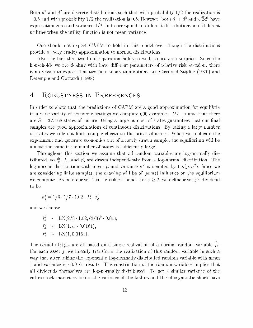
4.1 Random CARA

We randomly generate 100 examples of economies where all agents have constant absolute

risk aversion. For each example we draw the coe�cient of risk aversion �h, h = 1; 2; 3;

from a uniform distribution on the interval [0:5; 10]: Comparisons between the computed

equilibria and the CAPM predictions are depicted in the histograms of Figures 2a-d.6

Obviously CAPM predicts extremely well. The mean squared error always lies below

0:04 percent. In most cases it is around 0:5 � 10�4: The Pricing R2 exceeds 0:9999 in all

6The Pricing R2 is multiplied by 100 to avoid round-o� to 1.000 by our software.

16

0 0.5 1 1.5 2 2.5 3 3.5 4

x 10−4

0

2

4

6

8

10

12

14

16

18

20

Figure 2a: CARA: MSE.

99.99 99.991 99.992 99.993 99.994 99.995 99.996 99.997 99.998 99.9990

2

4

6

8

10

12

14

16

18

20

Figure 2b: CARA: 100� Pricing R2:

0.95 0.955 0.96 0.965 0.97 0.975 0.98 0.985 0.99 0.995 10

10

20

30

40

50

60

70

80

Figure 2c: CARA: Two-fund

separation agent 2.

0.98 0.982 0.984 0.986 0.988 0.99 0.992 0.994 0.996 0.998 10

10

20

30

40

50

60

70

Figure 2d: CARA: Two-fund

separation agent 3.

17

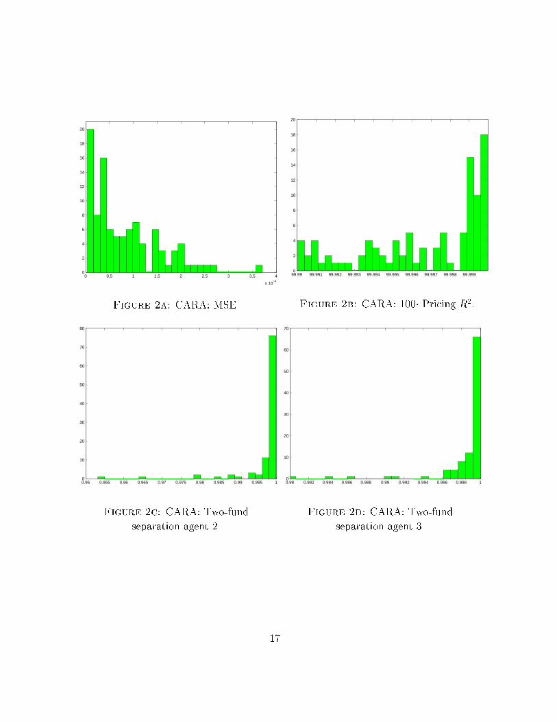
examples. The Two-fund R2 exceeds 0:99 in most cases. Compared to the single example

examined in Section 3, the results are slightly worse on average. Figure 3 clari�es that this

can be entirely explained by higher values for the average rate of risk aversion present in

the economy. The MSE increases with average risk aversion in the economy, as measured

by the harmonic mean of the �h's (it is well known that the harmonic mean is the right

measure for average risk aversion in an economy where all agents have constant absolute

risk aversion).

Although CAPM remains an excellent predictor for all cases examined so far, Figure 3

indicates that CAPM is a better tool in environments with lower average risk aversion. In

the light of this result one might be tempted to draw a parallel between our results and

the observation of Mehra and Prescott (1985) that realistic values of risk-aversion do not

produce a realistic equilibrium risk-premium. If the equilibrium returns of risky assets do

not change signi�cantly with small variations of agents' coe�cient of relative risk aversion

it can be expected that the cross section remains almost unchanged and that CAPM

(which predicts excess returns independently of preferences) provides a good prediction for

a variety of attitudes towards risk. Note, however, that this can only explain one side of

the phenomena - the question remains why the cross-section of returns can be described

by the assets' �'s.

4.2 Random CRRA

We now assume that all agents have constant relative risk aversion and we draw h, h =

1; 2; 3; from a uniform distribution on the interval [0:5; 10]: With mean household income

equal to 1; the degree of risk-aversion in the economy is similar to the CRRA-case examined

in Subsection 4.1. As before we compute 100 examples - Figures 4a-d report the analogues

of Figures 2a-d for the CRRA case.

Figure 4 shows that CAPM is an excellent predictor for the class of CRRA utility

functions, both in terms of pricing and in terms of two-fund separation. In most cases

MSE is around 1 � 10�4: The worst Pricing R2 found is 0:99995 and the worst Two-fund

R2 is 0:95:

The high values of the Pricing R2 provides very useful information for the pricing of

assets. Recall that the price of asset j is given by ��A �dj: Any vector that is highly correlatedwith ��A should lead to a similar price for asset j: In particular, when the Pricing R2 is

close to one, CAPM is bound to give almost exact equilibrium prices and the use of CAPM

leads to a low MSE.

4.3 Loss Aversion

To demonstrate that our results do not depend on state independent utility, we analyze

a class of utility functions that are state dependent and that are characterized by loss

aversion. Such utility functions get support from empirical work on the decision making

18

1 2 3 4 5 6 7 8 9 100

0.5

1

1.5

2

2.5

3

3.5

4x 10

−4

Harmonic Mean of Risk Aversion

MS

E o

f CA

PM

−P

ricin

g

Figure 3: MSE against Risk-Aversion for CRRA preferences.

19

0 0.5 1 1.5 2 2.5 3 3.5 4

x 10−4

0

5

10

15

Figure 4a: CRRA: MSE.

99.99 99.991 99.992 99.993 99.994 99.995 99.996 99.997 99.998 99.9990

5

10

15

20

25

30

35

40

45

50

55

Figure 4b: CRRA: 100� Pricing R2:

0.95 0.955 0.96 0.965 0.97 0.975 0.98 0.985 0.99 0.995 10

10

20

30

40

50

60

70

Figure 4c: CRRA: Two-fund

separation agent 2.

0.98 0.982 0.984 0.986 0.988 0.99 0.992 0.994 0.996 0.998 10

5

10

15

20

25

30

35

Figure 4d: CRRA: Two-fund

separation agent 3.

20

of agents. They are also claimed to be helpful in explaining the equity premium puzzle of

Mehra and Prescott (1985), see Benartzi and Thaler (1995).

We cannot use exactly the same utility functions as Benartzi and Thaler, as these are

not everywhere quasi-concave, and as a consequence a competitive equilibrium may not

exist. The important characteristic of loss-aversion is not so much the existence of non-

concavities, but a sharp decrease in utility when loosing income compared to the status

quo and only a mild increase in utility when gaining income. This is usually modeled by

a utility function that has a kink at the status quo.

We generate a utility function with loss aversion as follows. We identify the status quo

of an agent h in state s � 1 with ehs : Then loss aversion applies to making good or bad

investment decisions on the stock market. Consistent with Benartzi and Thaler (1995),

we want a Bernoulli function vhs such that limchs "ehs@vhs (c

hs ) = 2 limchs #e

hs@vhs (c

hs ): For each h;

we choose parameters h1 and h2 : When chs � ehs ; then vhs coincides with a CRRA utility

function with parameter of relative risk aversion h1 : When chs � ehs ; then vhs coincides with

a CRRA utility function with parameter of relative risk aversion h2 ; plus a term linear in

chs to get limchs "ehs@vhs (c

hs ) = 2 limchs #e

hs@vhs (c

hs); plus a constant ks to make vhs continuous.

More precisely, we assume that uh(ch) = vh0 (ch0) + �h

PSs=1 �sv

hs (c

hs), where

vh0 (ch0) = (ch0)

1� h1 =(1� h1 );

vhs (chs ) = (chs )

1� h2 =(1� h2 ) + (

2

1(ehs )

� h1 � (ehs )

� h2 )chs + ks; chs � ehs ;

vhs (chs ) = (chs )

1� h1 =(1� h1 ); chs � ehs ;

with

ks = 2

1� 2(ehs )

1� h2 +

h1 h2 + h1 � h2 h1 (1� h1 )

(ehs )1� h

1 :

The Bernoulli function vhs is continuous and is continuously di�erentiable except at ehswhere it has a kink. It can be shown that the coe�cient of relative risk aversion varies

continuously in chs and is given by ( h1 h2 (c

hs )

� h2 )=( h2 (e

hs )

� h1 � h1 (e

hs )

� h2 + h1 (c

hs )

� h2 ) if

chs � ehs , so it approaches h2 as chs ! 0: The coe�cient of relative risk aversion is given by

h1 if chs � ehs .

Since vhs is not di�erentiable at ehs it does not satisfy the assumptions under which the

algorithm has been shown to be convergent. We have to smooth out the kinks of the utility

function. We can do this by taking any eh�s ; eh+s such that eh�s < ehs < eh+s and de�ning

@vhs (chs ) =

eh+s � chseh+s � eh�s

@vhs (eh�s ) +

chs � eh�seh+s � eh�s

@vhs (eh+s ):

In principle, the parameter ks has to be adjusted to make vhs continuous. Since our algo-

rithm works entirely with �rst order conditions, this is of no concern to us. In the numerical

experiments we took eh�s = 0:95ehs and eh+s = 1:05ehs . For each example we take h1 = h2 =2

and we draw h2 , h = 1; 2; 3; from a uniform distribution on the interval [1; 6]. In this way

21

0 0.5 1 1.5 2 2.5 3 3.5 4

x 10−4

0

2

4

6

8

10

12

14

16

Figure 5a: LA: MSE.

99.99 99.991 99.992 99.993 99.994 99.995 99.996 99.997 99.998 99.9990

10

20

30

40

50

60

Figure 5b: LA: 100� Pricing R2:

0.95 0.955 0.96 0.965 0.97 0.975 0.98 0.985 0.99 0.995 10

5

10

15

20

25

30

35

40

45

Figure 5c: LA: Two-fund

separation agent 2.

0.98 0.982 0.984 0.986 0.988 0.99 0.992 0.994 0.996 0.998 10

5

10

15

20

25

30

35

40

45

50

Figure 5d: LA: Two-fund

separation agent 3.

22

�fty economies are randomly generated. The outcomes of our computations are presented

in Figures 5a-d.

It turns out that CAPM is an extraordinarily good predictor for the case with loss

aversion. The results seem to be even better than for the CRRA and CARA cases examined

before. In most cases, MSE is below 1 �10�4; Pricing R2 exceeds 0:99999; and the Two-fund

R2 exceeds 0:98: If we take into account that the examples with loss aversion are such that

the degree of risk aversion is lower on average than before, the Pricing R2 is comparable

to the one found for CRRA and CARA preferences.

5 Robustness in Return Processes

We now �x agents' preferences to exhibit constant relative risk aversion and choose 1 = 6;

2 = 4; and 3 = 2: We test the robustness of our results to variations in the distributions

of endowments and assets. We consider three di�erent families of return processes and

compute 100 randomly generated examples within each class. We show the histograms of

MSE, Pricing R2; and Two-fund R2 of agents 2 and 3.

5.1 Uniform Returns

In order to verify whether our results depend on the assumption of log-normal shocks, we

now assume that all shocks are uniformly distributed. We also allow for some variation in

the ratio of labor income to total income, in the variance of the factor and in the variance

of the idiosyncratic shocks.

We start each example by randomly generating parameters a1; a2; a3 and a4; where

a1 � U(1:02 � 0:5; 1:02 � 0:9);a2 � U(1:02 � 1:1; 1:02 � 1:5);a3 � U(�0:5;�0:1);a4 � U(0:1; 0:5):

Given a realization for a1; : : : ; a4; we continue the construction of the economy by taking

independent drawings for lhs ; fs and "js; where

lhs � U(2=3 � 0:8; 2=3 � 1:24);fs � U((a1 � a2)=2; (a2 � a1)=2);

"js � U(a3; a4):

Finally, dividends are determined by

djs = 1=3 � 1=7 � (a1 + a2

2+pcjfs + "js):

Given the realizations for the parameters a1 and a2; 1=3 � 1=7 � (a1 + a2)=2 equals expected

dividends from asset j: The realization of the factor belongs to the interval [(a1�a2)=2; (a2�

23

a1)=2] and the realizations of the idiosyncratic shocks to the interval [a3; a4]: The expected

labor income and the variance of labor income are taken as before.

Figures 6a-d show that the ability of CAPM to predict portfolio-holdings and excess

returns is robust to the exact speci�cation of the distribution of shocks. The results are very

close to the ones obtained for the base case with log-normal shocks examined in Section 3,

where the average degree of risk aversion in the economy is similar.

5.2 More Factors

One might wonder whether our results are not simply due to the fact that we have all risky

assets being in uenced by a single common factor. In fact, it is possible to derive CAPM

as a special case of APT where there is only one factor, see for instance Connor (1984).

However, such a derivation requires an uncountable number (or at least very large number)

of assets to diversify the idiosyncratic shocks away. The importance of idiosyncratic shock

is quite substantial in our economies with only seven risky assets. Moreover, usually factors

enter linearly in the de�nition of an asset's pay-o�, which is not always the case in our

economies. It seems therefore not likely that our results are due to the single factor set-up.

Other suspicious elements of the set-up we used so far are that factor loads are dis-

tributed very symmetrically and balanced, and that the importance of idiosyncratic shocks

is the same for all assets. Finally, we consider a wider range for the variance of the entire

stock market.

In this subsection we generate a number of economies where risky assets depend on two

factors, f and bf; and factor loads for each one of the assets are randomly drawn. On top

of this, also the importance of the idiosyncratic shock is randomly determined.

We start each example by randomly generating, for each asset j = 2; : : : ; J; parameters

cj; bcj; and ij: These parameters represent the load in factor 1, the load in factor 2 and the

importance of the idiosyncratic shock. More speci�cally it holds that

cj � U(0; 2);bcj � U(0; 2);

ij � U(0; 4):

Labor income, the two factors and assets' idiosyncratic shocks are independently log-

normally distributed, so lhs ; fs;bfs; and "js are drawn from a log-normal distribution,

lhs � LN(2=3 � 1:02; (2=3)2 � 0:01);f js � LN(1; cj � 0:0161);bf js � LN(1; bcj � 0:0161);"js � LN(1; ij � 0:0161):

Finally, dividends are determined by

djs = 1=3 � 1=7 � 1:02 � f js � bf js � "js:24

0 0.5 1 1.5 2 2.5 3 3.5 4

x 10−4

0

2

4

6

8

10

12

Figure 6a: Uniform: MSE.

99.99 99.991 99.992 99.993 99.994 99.995 99.996 99.997 99.998 99.9990

5

10

15

20

25

30

Figure 6b: Uniform: 100� Pricing R2:

0.95 0.955 0.96 0.965 0.97 0.975 0.98 0.985 0.99 0.995 10

5

10

15

20

25

30

35

40

Figure 6c: Uniform: Two-fund

separation agent 2.

0.98 0.982 0.984 0.986 0.988 0.99 0.992 0.994 0.996 0.998 10

5

10

15

20

25

30

Figure 6d: Uniform: Two-fund

separation agent 3.

25

The way to generate f js ; j = 2; : : : ; J; from a single realization of a normally distributed

random variable is the same as in Section 3. The same applies to the other factor.

From Figure 7 we may conclude that the one factor framework is certainly not the

driving force that makes CAPM work. Also in the two factor set-up, for a variety of factor

loads, with assets that are di�erent in the importance of the idiosyncratic shocks, CAPM

turns out to be an excellent model.

5.3 Options

Since markets are incomplete the introduction of an option on one of the assets will gener-

ally change all equilibrium prices (see Detemple and Selden (1991)). Therefore one might

expect that the introduction of an option worsens CAPM-pricing considerably. Further-

more, given the robustness of CAPM in the earlier examples, it is interesting to see if it

is possible to give an equilibrium pricing formula for options in incomplete markets via

CAPM.

Another reason to introduce an option is that this is an asset with the capacity to

seriously alter the higher order moments of an asset portfolio. One possible explanation

for our results obtained so far is that asset markets are very incomplete, which makes it

di�cult for households to change the higher order moments of the returns of their portfolios.

Although households care for higher order moments, the mix of marketed assets makes it

di�cult to a�ect the higher order moments. With the introduction of an option this clearly

changes. Agents have then a possibility to limit downwards risk, which is exactly the kind of

risk agents with CRRA utility functions are concerned about, but mean-variance optimizers

are not.

In order to investigate this issue more closely we introduce a call option on the most

risky asset. Speci�cally we have a 9-th security which pays max(djs�X; 0) in state s, with

X the strike price of the call option.

Suppose we consider the uniquely determined equilibrium pricing vector ��A of the

economy without the option, and we use this pricing vector to price the option. Given the

reasoning of the previous paragraph, at those prices one would expect the call option (in

combination with the bond) to be more attractive to the agents than the stock, exactly

because of the higher order moments. So the equilibrium price of the call option should be

higher than the one computed by CAPM-pricing, in order to make that asset less appealing.

As a consequence, the expected equilibrium return of the call option should be less than

the one predicted by CAPM.

To examine di�erent options, we draw X out of the uniform distribution for each

example. To avoid options that are either too far in or too far out of the money we

determine in each example the minimal dividend paid out by asset 8; d8 = mins=1;:::;S d8s;

and the maximal dividend paid out, d8= maxs=1;:::;S d

8s: We then draw X out of a uniform

distribution on [0:5 � (1:02 + d8); 0:5 � (1:02 + d8)]: Note that 1:02 is the expected dividend

of asset 8. The strike price is always between the average of the minimal dividend and the

26

0 0.5 1 1.5 2 2.5 3 3.5 4

x 10−4

0

5

10

15

20

25

Figure 7a: Two-factor: MSE.

99.99 99.991 99.992 99.993 99.994 99.995 99.996 99.997 99.998 99.9990

10

20

30

40

50

60

Figure 7b: Two-factor: 100� PricingR2:

0.95 0.955 0.96 0.965 0.97 0.975 0.98 0.985 0.99 0.995 10

10

20

30

40

50

60

70

Figure 7c: Two-factor: Two-fund

separation agent 2.

0.98 0.982 0.984 0.986 0.988 0.99 0.992 0.994 0.996 0.998 10

10

20

30

40

50

60

70

80

Figure 7d: Two-factor: Two-fund

separation agent 3.

27

expected dividend, and the average of the expected dividend and the maximal dividend.

The results are given in Figures 8a-d.

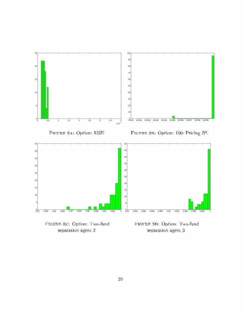
The MSE in Figure 8 refers to the MSE of the pricing of the stocks only. The option

is analyzed in detail in Figure 9. It turns out that the MSE, and the Two-fund R2 are

comparable to the ones given before. The Pricing R2 is somewhat less good than before,

but is still excellent. Surprisingly, we have found no systematic e�ect of the introduction

of the option on the price of asset 8. In some examples the introduction of an option raised

the price above the CAPM-prediction, in others it has been lower.

Figure 9 analyzes the pricing of the option by CAPM. According to CAPM, a call option

is a very risky asset. It has zero pay-o�s in bad states of nature, and very high in good states

of nature. The covariance of a call option with the market portfolio is very high, which is

also clear from Figure 9, where it is shown that the option's � varied from 5 to 35 in the

economies generated. Notice that, as we expected, there is indeed an over-prediction of the

expected return of an option by CAPM. In all economies generated, CAPM underpriced

the call option. The misprediction was relatively small when the option's � is low, say

below 10, but may get quite severe for call options with a very high strike price, which

are the ones with a high �: Notice, however, that a higher � of an option also corresponds

to a higher excess return, which makes the relative misprediction less bad. Still, the over-

prediction of call option returns is more than linearly increasing in an option's �; whereas

the excess return itself is still roughly linear.

It is surprising that the Pricing R2 and the MSEs of stocks remained so good in all

economies, even when the option was sometimes seriously under-priced by CAPM. In fact,

it may even be perceived as an inconsistency that the PricingR2 is virtually exactly correct,

and the option is seriously mispriced. Indeed, when CAPM-pricing is highly correlated with

��A; almost all assets are priced very well. The only exceptions are those like options with

a very high strike price. Such an asset pays o� in a few (less than 10) states of the 32,768

only. A high correlation with ��A is not inconsistent with a fairly di�erent state price in a

negligible fraction of states only.

6 Interpretation and Conclusion

In order to show that the CAPM-pricing formula holds, one needs strong assumptions either

on preferences or on dividends and endowments (see Berk (1996)). However, examining the

robustness of CAPM by computing equilibria, we �nd that CAPM provides an excellent

approximation to equilibrium excess returns and portfolio-holdings for a wide variety of

preferences, dividends and endowments.

This result is very puzzling for two separate reasons. First, there is no a priori reason

why in the absence of mean-variance prefernces or normal returns, the CAPM-pricing

formula should provide a good approximation to actual equilibrium prices if there is only

one agent in the economy or if markets are complete (which is observationally equivalent).

28

0 0.5 1 1.5 2 2.5 3 3.5 4

x 10−4

0

5

10

15

20

25

Figure 8a: Option: MSE.

99.99 99.991 99.992 99.993 99.994 99.995 99.996 99.997 99.998 99.9990

10

20

30

40

50

60

70

80

90

100

Figure 8b: Option: 100� Pricing R2:

0.95 0.955 0.96 0.965 0.97 0.975 0.98 0.985 0.99 0.995 10

5

10

15

20

25

30

35

40

45

Figure 8c: Option: Two-fund

separation agent 2.

0.98 0.982 0.984 0.986 0.988 0.99 0.992 0.994 0.996 0.998 10

5

10

15

20

25

30

35

40

45

50

Figure 8d: Option: Two-fund

separation agent 3.

29

5 10 15 20 25 30 350

0.02

0.04

0.06

0.08

0.1

0.12

Figure 9: Option: over-prediction of return against option's �:

30

Secondly one would expect the presence of heterogeneous agents and incomplete �nancial

markets to alter the pricing implications of consumption based pricing models signi�cantly.

We compute the complete market equilibirum for the examples considered. In almost

all of the cases the complete markets pricing errors lie even below the incomplete market

errors. In order to understand this �rst puzzle, consider the simplest possible setup with a

single agent who has log-utility and no labor-income. Suppose that the dividends of stocks

j = 2; :::; 8 are given by

djs = �j(�+ "1s) + "js;

where all " are iid. From Section 2 we know that if we normalize e0 = 1 the pricing errors

of the CAPM pricing formula for asset j is given by

� = Edj � E(dj=~e)

E(1=~e)� (E~e� 1

E(1=~e))cov(dj; ~e)

var(~e)

The results in this paper might become a little more plausible if one realizes that if factor-

weights (�j)j=2;:::;8 are such thatP8

j=2 �j = 1 then � = 0. Substituting for dj and ~e, since

there are 7 stocks and sincecov(dj ;~e)var(~e) = (�j + 1)=8 we obtain

� = �j��E

�j(�+�1)+�j

�+P

8

i=1�i

E 1

�+P

8

i=1�i

�

0B@�� 1

E 1

�+P

8

i=1�i

1CA (�j + 1)=8

In order to show that � = 0 the crucial insight is that

E�j

�+P

8

i=1�i� 1=8

E 1

�+P

8

i=1�i

+ 1=8� = 0:

ForP8

j=2 �j 6= 1, � 6= 0 but the resulting pricing errors are small. As long as the coe�cient

of relative risk aversion remains low the pricing errors remain low if we vary the utility

functions (see Figure 3).

However, while this argument shows that given our calibration one would expect CAPM

to provide a good approximation to prices if there is only a single agent, one has to compute

equilibria in order to assess how well CAPM predicts equilibrium prices in economies

with heterogeneous agents and incomplete markets. Our current computational experience

suggests that CAPM is an excellent tool to price assets in realistically calibrated economies

with incomplete markets. The results seem to be robust for a wide variety of cases. The

form of the utility functions, the distribution of the shocks, the number of factors, and the

introduction of options do not a�ect our results. The question which then arises out of the

analysis in this paper is why the presence of incomplete markets does not have signi�cant

e�ects on cross-sectional returns.

31

References

[1] Benartzi, S., and R.H. Thaler (1995), \Myopic Loss Aversion and the Equity Premium

Puzzle," Quarterly Journal of Economics, 440, 73-92.

[2] Berk, J.B. (1997), \Necessary Conditions for the CAPM," Journal of Economic The-

ory, 73, 245-257.

[3] Brown, D.J., P.M. Demarzo, and B.C. Eaves (1996), \Computing Equilibria When

Asset Markets Are Incomplete," Econometrica, 64, 1-27.

[4] Cass, D., and J.E. Stiglitz (1970), \The Structure of Investor Preferences and Asset

Returns, and Separability in Portfolio Allocation: A Contribution to the Pure Theory

of Mutual Funds," Journal of Economic Theory, 2, 122-160.

[5] Chamberlain, G. (1983), \A Characterization of the Distributions That Imply Mean-

Variance Utility Functions," Journal of Economic Theory, 29, 185-201.

[6] Connor, G. (1984), \A Uni�ed Beta Pricing Theory," Journal of Economic Theory,

34, 13-31.

[7] Detemple, J.B., and P. Gottardi (1998), \Aggregation, E�ciency and Mutual Fund

Separation in Incomplete Markets," Economic Theory, 11, 443-455.

[8] Detemple, J.B., and L. Selden (1991), \A General Equilibrium Analysis of Option and

Stock Market Interactions," International Economic Review, 32, 279-303.

[9] Fama, E.F. and K.R. French (1992), \The Cross-Section of Expected Stock Returns,"

Journal of Finance, 47, 427-465.

[10] Feldstein, M.S. (1969), \Mean-Variance Analysis in the Theory of Liquidity Preference

and Portfolio Selection," Review of Economic Studies, 36, 5-12.

[11] Garcia, C. and W. Zangwill (1981), Pathways to Solutions, Fixed Points, and Equi-

libria, Prentice Hall, Englewood Cli�s.

[12] Geanakoplos, J.D., and H.M. Polemarchakis (1986), \Existence, Regularity, and Con-

strained Suboptimality of Competitive Allocations when the Asset Market is Incom-

plete," in W.P. Heller, R.M. Starr, and D.A. Starrett (eds.), Uncertainty, Information

and Communication: Essays in Honor of K.J. Arrow, Vol. III, Cambridge University

Press, Cambridge, 65-96.

[13] Geanakoplos, J., and M. Shubik (1990), \The Capital Asset Pricing Model as a General

Equilibrium With Incomplete Markets," The Geneva Papers on Risk and Insurance,

15, 55-72.

32

[14] Gottardi, P., and T. Hens (1996), \The Survival Assumption and Existence of Com-

petitive Equilibria when Asset Markets are Incomplete," Journal of Economic Theory,

71, 313-323.

[15] Hens, T. (1991), Structure of General Equilibrium Models with Incomplete Markets,

Doctoral Dissertation, University of Bonn.

[16] Herings, P.J.J. and F. Kubler (2000), \Computing Equilibria in the Finance Version

of the General Equilibrium Model with Incomplete Asset Markets," working paper.

[17] Judd, K.L. (1997), \Computational economics and economic theory: Subsitutes or

complements ?" Journal of Economic Dynamics and Control, 21, 907-942.

[18] Lintner, J. (1965), \The Valuation of Risky Assets and the Selection of Risky Invest-

ments in Stock Portfolios and Capital Budgets," Review of Economics and Statistics,

47, 13-37.

[19] Magill, M.J.M., and M. Quinzii (1996), Theory of Incomplete Markets, MIT Press,

Cambridge.

[20] Markowitz, H.M. (1959), Portfolio Selection: E�cient Diversi�cation of Investment,

Yale University Press, New Haven.

[21] Mehra, R., and E.C. Prescott (1985), \The Equity Premium, A Puzzle," Journal of

Monetary Economics, 15, 145-161.

[22] Oh, G. (1996), \Some Results in the CAPM with Nontraded Endowments," Manage-

ment Science, 42, 286-293.

[23] Owen, R., and R. Rabinovitch (1983), \On the Class of Elliptical Distributions and

Their Applications to the Theory of Portfolio Choice," Journal of Finance, 38, 745-

752.

[24] Ross, S.A. (1978), \Mutual Fund Separation in Financial Theory: The separating

Distributions," Journal of Economic Theory, 17, 254-286

[25] Schmedders, K. (1998), \Computing Equilibria in the General Equilibrium Model

with Incomplete Asset Markets," Journal of Economic Dynamics and Control, 22,

1375-1401.

[26] Sharpe, W.F. (1964), \Capital Asset Prices: A Theory of Market Equilibrium under

Conditions of Risk," Journal of Finance, 19, 425-442.

[27] Tobin, J. (1958), \Liquidity Preference as Behavior toward Risk," Review of Economic

Studies, 25, 65-86.

33

[28] Willen, P.T. (1997), A Model which Allows for Comparison of Di�erent Levels of

Market Incompleteness, mimeo, Yale University, New Haven.

34