THE PRODUCTION, APPLICATIONS AND ECONOMIC STUDY OF

ACTIVATED CARBON FOR LARGE SCALE PRODUCTION INCLUDING AN

EDUCATIONAL STUDY ON UNDERGRADUATE LABORATORY MODULES

____________________________________

A Thesis presented to

The Faculty of the Graduate School

At the University of Missouri

_____________________________________

In Partial Fulfillment

Of the Requirements for the Degree

Master of Science

___________________________________________________________

By

MICHELLE JI

Dr. Galen Suppes, Thesis Advisor

DECEMBER 2010

The undersigned, appointed by the dean of the Graduate School, have examined the thesis entitled

THE PRODUCTION, APPLICATIONS AND ECONOMIC STUDY OF ACTIVATED

CARBON FOR LARGE SCALE PRODUCTION INCLUDING AN EDUCATIONAL

STUDY ON UNDERGRADUATE LABORATORY MODULES

presented by Michelle Ji,

a candidate for the degree of master of science,

and hereby certify that, in their opinion, it is worthy of acceptance.

Professor Galen Suppes

Professor Paul Chan

Professor Sheila Grant

…to the Chemical Engineering Department, University of Missouri.

ii

Acknowledgements

I would like to express my sincere gratitude to my advisor, Dr. Galen Suppes for

the opportunity to work on these projects, and for his support, encouragement, and

guidance in developing these experiments.

I would also like to thank Dr. Sheila Grant for all of her encouragement and

direction during my undergraduate years and for serving as a thesis committee member.

I would like to thank Dr. Paul Chan for his insight and assistance in my graduate

studies and for serving as a thesis committee member.

This work could not have been completed without the help of my co-researchers,

and I would like to show my deepest appreciation to Bryan Sawyer, Michael Gordon,

Ramsey Hilton, Frank Kirkley and Ali Tekeei for their patience and dedication.

I would like to thank my parents, Ya-Li Tian and Jian- Min Ji, my sister, Diana Ji,

and my grandparents, Zhong –Mei Chen and Jia-He Tian for their unconditional love and

support in my decision to pursue higher education.

And lastly I would like to thank my friends, Alana Zhu, Stephanie Song, and

Chris Gu for all of their encouragement and support throughout the years.

Michelle Ji

iii

Disclaimer

This thesis includes estimates of equipment costs, operating costs, and

profitability. These are only estimates prepared for discussion purposes. These estimates

are not intended to represent an accurate assessment of the costs or profitability for any

application.

iv

TABLE OF CONTENTS

ACKNOWLEDGEMENTS……………………………………………………………..ii

DISCLAIMER………………………………………………………………………… iii

LIST OF TABLES………………………………………………………………………vii

LIST OF FIGURES……………………………………………………………………...viii

ABSTRACT……………………………………………………………………………...x

CHAPTERS……………………………………………………………………………….1

1. THE CARBON PROJECT………………………………………………………..1

1.1 Introduction of Natural Gas……………………………………………….1

1.2 Types of Natural Gas Storage and Transportation………………………...3

1.2.1 Liquefied Natural Gas (LNG)……………………………………..3

1.2.2 Compressed Natural Gas (CNG)………………………………….4

1.2.3 Adsorbed Natural Gas (ANG)…………………………………….4

1.3 Activated Carbon………………………………………………………….6

1.3.1 Introduction……………………………………………………….6

1.3.2 Activated Carbon and Adsorption………………………………...7

1.3.3 Other Applications of Activated Carbon………………………….7

1.3.4 Activated Carbon Production……………………………………..8

1.3.4.1 Materials and Experimental Procedure………………..8

1.3.5 Activated Carbon Mass Balance…………………………………11

1.4 Adsorbed Natural Gas Progress and Goals………………………………12

v

1.5 Introduction to Economical Analysis…………………………………….12

1.5.1 Base Case Scenario………………………………………………12

1.5.2 Large Scale Carbon Production………………………………….13

1.5.2.1 Cost of Materials and Size of Equipment……………13

1.5.2.2 Annual Operating Cost………………………………16

1.5.2.3 Net Present Value Over Ten Years…………………..17

1.5.2.4 Cost of Carbon Production with 70% Recycle………18

1.6 Conclusion……………………………………………………………….20

2. INTRODUCTION OF BATTERY MODULE………………………………….21

2.1. Importance of Battery Technology and Introduction of Modules……….21

2.2. Objectives………………………………………………………………..22

2.3. Energy Balance for Battery-Resistor Circuit Module Description………23

2.3.1. Storage Capabilities and Equipment……………………………..24

2.3.2. Description of Hardware and Circuitry…………………………..25

2.3.3. Schematic of Resistor Bank……………………………………...26

2.4. Data Acquisition Software……………………………………………….27

2.5. LabVIEW BatteryResistorEnergyBalance.VI Program Explanation……27

2.6. Operating Procedures…………………………………………………….28

3. LABORATORY TEACHING MODULES……………………………………..29

3.1. Introduction………………………………………………………………29

3.2. Project 1: Battery Resistor Energy Balance……………………………...29

3.2.1. Laboratory Operational Procedures……………………………...30

vi

3.2.2. Governing Equations…………………………………………….32

3.2.3. Modeling Data…………………………………………………...32

3.2.4. Other Applications……………………………………………….35

3.2.5. Sample Outline for Project 1: Battery Resistor Energy Balance...36

3.2.6. MatLAB Codes for Project 1: Battery Resistor Energy Balance...39

3.3. Project 2: Evaluating the Internal Resistance of a Battery………………41

3.3.1. Laboratory Operating Procedures………………………………..41

3.3.2. Sample Outline for Project 2……………………………………..44

3.4. Project 3: Diffusion and Permeability in a Manganese Dioxide-Zinc

Battery……………………………………………………………………45

3.4.1. Laboratory Operating Procedures………………………………..46

3.4.2. Separator Material for Cathode and Anode……………………...48

3.4.3. Diffusivity and Permeability Results…………………………….49

3.4.4. Sample Outline for Project 3……………………………………..50

3.5. Student Feedback………………………………………………………...53

3.6. Conclusion.………………………………………………………………53

REFERENCES…………………………………………………………………………..54

vii

LIST OF TABLES

Table 1-1 Sample BET measurements for carbons. 3K Surface Area σ= 200, 3K

Porosity σ=0.025…………………………………………………………………………10

Table 1-2 Sample mass balance on activated carbon process: 3K, 790°C, 1 hour……..11

Table 1-3 Materials for the production of 2000 lbs/day of activated carbon…………...13

Table 1-4 Cost estimation for the production of 2000 lbs/day of activated carbon……..13

Table 1-5 List of equipment used for activated carbon production……………………..14

Table 1-6 Cost and size of equipment for carbon production without recycle………...15

Table 1-7 Annual utilities cost summary of equipment used for carbon production…..16

Table 1-8 Equivalent annual operating cost for carbon production……………………16

Table 1-9 Summary of total purchase costs of process equipment by equipment type..17

Table 1-10 Net Present Value calculations for the production of activated carbon

(without recycle) in millions of dollars…………………………………………………..18

Table 1-11 Cost and size of equipment for carbon production with 70% recycle……..19

Table 3-1 Sample parameters used model the resistor temperature versus time. ………33

viii

LIST OF FIGURES

Figure 1-1 Block flow diagram of carbon production…………………………………... 9

Figure 1-2 Process flow diagram of activated carbon production……………………..14

Figure 2-1 Energy Balance for Battery-Resistor Circuit module……………………....23

Figure 2-2 Storage cabinet for stand-alone laboratory modules………………………..24

Figure 2-3 Close up images of module, including from left to right: AA battery holder;

expanded image of 1-ohm resistor with thermocouple attached with shrink wrap; circuit

board with 1-ohm resistor, two resistor banks, and knobs for selecting resistance from

two resistor banks; and switches used to select locations for voltage measurements…...25

Figure 2-4 Schematic of the experimental system which shows the different resistors in

series and switch settings for voltage measurements…………………………………….26

Figure 2-5 Front panel view of LabVIEW BatteryResistorEnergyBalance.VI program..27

Figure 3-1 A plot of the resistor and battery temperature profile with a 3 Ohm total

resistor…………………………………………………………………………………….33

Figure 3-2 A plot of the resistor temperature with superimposition of modeling results

(left) and voltage profile of the battery operating with a 3 Ohm total resistor (right)…...34

Figure 3-3 Schematic of resistor bank on module………………………………………38

Figure 3-4 Schematic of a battery as a voltage source in series with an internal

resistance…………………………………………………………………………………41

ix

Figure 3-5 Example results from PROJECT 2 and equation 3-6 for evaluating the

internal resistance of a battery. The data are for different circuit resistances evaluated

with the experimental module……………………………………………………………43

Figure 3-6. Model illustration of a battery as a voltage source in series with an internal

resistance…………………………………………………………………………………44

Figure 3-7 Pictorial representation of a compression cell used for the assembly of MnO2

– Zn batteries (left) with picture of assembled cell (middle) and an assembled cell with

weight to provide compression (right)…………………………………………………...45

Figure 3-8 Graph of results showing proposed trend of decreasing voltage with

increasing resistance of separator between electrodes. The numbers indicate the number

of layers of filter paper between the electrodes………………………………………… 50

Figure 3-9 Schematic of resistor bank…………………………………………………..52

x

THE PRODUCTION, APPLICATIONS AND ECONOMIC STUDY OF

ACTIVATED CARBON FOR LARGE SCALE PRODUCTION INCLUDING AN

EDUCATIONAL STUDY ON UNDERGRADUATE LABORATORY MODULES

Michelle Ji

Dr. Galen Suppes, Thesis Supervisor

ABSTRACT

The production of activated carbon was evaluated using a biomass feed stock,

corn cobs, as a precursor. The importance of the carbonization process and activation

process are discussed and how nanopores and its unique surface chemistry allow

activated carbon to perform advantageously in the transportation of natural gas.

Adsorbed natural gas transportation is a valuable technique because of its ability to gain

access and utilize methane from currently unavailable resources by conventional

methods. A design approach was proposed and evaluated using the applications of

activated carbon to transport natural gas including economic analyses on the large scale

production of activated carbon.

In addition, an experimental learning module was developed to study the mass

and energy balance involved with operation of an AA Alkaline battery under a load

current. An extension of the module allows evaluation of laboratory assembled batteries

using granular anodic/cathodic materials. The system allows load resistance to be varied

and measures voltage and temperature. The importance of batteries and the integration of

chemical engineering education is discussed involving the battery- resistor circuit

module.

1

CHAPTER 1

THE CARBON PROJECT

1.1. Introduction of Natural Gas

Natural gas is a co-product of crude oil production and provides nearly one-fifth

of all the world’s primary energy requirements. It was discovered in Fredonia, New York

in 1821, and initially it was used as fuel in areas immediately surrounding the gas fields.

Since then, the construction of long -distance, large diameter pipelines have been able to

bring the supply of gaseous fuel to domestic, commercial, and industrial consumers to

areas miles away from the gas fields[1]. The turning point in the natural gas industry

occurred after World War II due to increases in natural gas consumption for residential,

commercial, industrial, and power generation. Several contributors led to this growth

including the development of new markets, the replacement of coal, using natural gas in

making petrochemicals and fertilizers, and the growing demand for low-sulfur fuels[2].

Natural gas is a mixture of hydrocarbons and other impurities. Methane is the

main component in natural gas followed by ethane, propane, butane, pentanes, and small

amounts of hexanes, heptanes, octanes, and other heavier gases[1]. The impurities

present in natural gas include carbon dioxide, hydrogen sulfide, nitrogen, water vapor,

and heavier hydrocarbons. The composition of natural gas varies from each stream, and

each gas stream produced from a natural gas reservoir can change its composition as it is

depleted[2]. The propane and heavier hydrocarbons are usually removed to be

additionally processed because of their high market value, so the natural gas that is

2

available for consumers is mainly composed of a mixture of methane and ethane with a

small percentage of propane.

The importance of natural gas has increased significantly in the last 25 years

because of the widening infrastructure of pipelines and compressor stations that are being

developed, especially transnational pipelines. Gas has also been established as an

environmentally friendly fuel that burns much more efficiently than oil or coal. The only

by-products released from natural gas if burned correctly are carbon dioxide and water.

Natural gas is also sold at a discounted price in terms of energy equivalence since 6

MSCF (thousand standard cubic feet) of gas is equal to one barrel of oil. As a price

comparison, 8-10 MSCF (thousand standard cubic feet) of gas is equivalent to one barrel

of oil[2]. Natural gas is also being used as a motor fuel because it burns cleaner than

traditional gasoline or diesel engines. Many vehicles are being retrofitted to use natural

gas as an alternative to gasoline or diesel, and these engines are proving to be

environmentally friendly and efficient[3].

There are currently two conventional types of natural gas storage and

transportation in use, either in the form of liquefied natural gas or compressed natural

gas. This chapter proposes an alternative method described as adsorbed natural gas using

activated carbon to deliver natural gas that is unreachable by pipelines or other

conventional methods. These gas fields are referred to as “stranded” natural gas either

physically or economically. It is physically stranded because of its remote or

geographically challenging location or economically stranded because the amount of gas

produced is not sufficient enough to build a multi-million dollar facility for processing

and distribution.

3

Adsorbed natural gas uses activated carbon, which is a highly adsorbent,

nanoporous material to bind to the methane molecules, and the carbon is often referred to

as a “sponge for natural gas[4].” Adsorbed natural gas is a viable alternative in natural

gas storage and transport, and its economic feasibility including the large scale

production of activated carbon is discussed in this chapter.

1.2. Types of Natural Gas Storage and Transportation

1.2.1. Liquefied Natural Gas (LNG)

The energy demands of Japan, Western Europe, and the United States were

growing rapidly and could not be satisfied without importing natural gas. In the 1930s,

the use of refrigeration to liquefy dry natural gas to reduce its volume was introduced in

Hungary, and later used in the United States for moving gas from the gas fields in

Louisiana to Chicago[1]. This liquefaction process became economically attractive to

transport natural gas across oceans by tankers since the gas is reduced to about one six-

hundredth of its original volume and the non-methane components are largely eliminated.

Liquefied Natural Gas (LNG) technology also requires handling at very low temperatures

around 108.15 K, and at the receiving terminals, LNG is reconverted into a gaseous phase

using a regasifying plant and fed into the conventional gas distribution process of the

importing country[5]. LNG can also be stored in insulated tanks or subsurface storages

for future use. However, for LNG to be economically successful, certain parameters need

to be satisfied. First, the location where the natural gas is produced should have reserves

capable of producing 25 to 30 times the annual capacity of the plant. Second, as a rule of

thumb, the cost of building a liquefaction plant ranges from $225 to $675 million for 100

MMSCFD (million standard cubic feet per day) capacity. Third, the tankers built for

4

LNG transportation requires special linings and double hulls. It is estimated that a 3 BCF

(billion cubic feet) tanker costs $260 million and transportation costs increase linearly

with distance. And lastly, the LNG can only be distributed into specialized terminals,

and the cost of re-gasification plants can run up to several hundred million dollars[2].

1.2.2. Compressed Natural Gas (CNG)

The major transportation of natural gas is carried through pipelines. On average,

over 12,000 miles of new gas pipelines are completed per year within the last five to six

years, most being transnational[2]. Currently, the main transportation of gas is carried

out by using compressed natural gas. Compressed natural gas (CNG) can be used as a

substitute for gasoline or diesel, and it is made by compressing natural gas to less than

one percent of its volume at standard atmospheric pressure. It is stored and transported in

heavy, thick –walled, cylindrical containers at pressures up to 3600 psig[6]. Another use

for CNG is in internal combustion engines to power vehicles. CNG vehicles require

more space for fuel storage than gasoline powered vehicles due to the physical properties

of compressed gas, rather than a liquid like gasoline so there are challenges in creating

space or maintaining free space in the construction of CNG vehicles[7]. Another

consideration is the structural strength of the vehicle to withstand the heavy components

of the storage tanks for compressed natural gas. The high cost of cylinders and the high

pressure facilities limit the practical use of CNG in natural gas fuelled vehicles.

1.2.3. Adsorbed Natural Gas (ANG)

Adsorbed natural gas (ANG) provides a method of storing gas at a lower

compression using activated carbon. It is a simpler process than liquefied natural gas or

5

compressed natural gas because it does not require the use of refrigeration or significant

supplementary equipment. Activated carbon is a form of carbon that has been

chemically processed in order to create a dense network of micropores and nanopores to

increase its surface area for adsorption. The primary advantage of ANG technology over

CNG is the low pressure. Activated carbon can be packed into storage vessels and filled

with pressurized methane at 500 psig at ambient temperatures compared to 3600 psig for

the CNG process[8]. Natural gas is attracted to the porous activated carbon by Van der

Waals forces and later, the gas can be desorbed when subjected to higher temperatures or

higher pressures[9]. This type of storage is appealing due to the fact that gas can be

stored at lower pressures in a lower volume environment, which would be more

convenient and economically efficient for transportation because it would use lighter,

smaller tanks. Methane can be stored with relatively high energy density on activated

carbon at ambient temperatures and low pressure (~500 psig), so the lower pressures

would allow the use of larger containers for transportation to reduce the amount of

wasted space and weight of the transport module[10].

For bulk storage applications, ANG technology is essentially dependent on the

cost of the adsorbing material. However, the price of high performing carbons tends to

increase disproportionally to the advantage gained in storage capacity[10]. For ANG

applications, the capacity of the carbon is expressed as storage per unit volume in terms

of volume per volume stored (v/v). Vigorous research efforts have been utilized to

produce activated carbons capable of storing up to 190 volumes of gas per volume of

storage space (v/v) at pressures of approximately 500 psig. The focus of this chapter will

6

be on the large scale production of activated carbon to transport stranded natural gas in

the form of adsorbed natural gas (ANG).

1.3. Activated Carbon

1.3.1. Introduction

Activated carbon includes a wide range of processed amorphous carbon-based

materials with a microcrystalline structure. They are known for their highly developed

porosity and extensive surface area. Carbon is the major component of activated carbon

and is present to the extent of 87 to 97%. Other elements are also present such as

hydrogen, nitrogen, sulfur, and oxygen[11]. The most widely used activated carbon

adsorbents have a specific surface area of 800 to 1500 m2g-1 and a pore volume range of

0.20 to 0.60 cm3g-1[9]. The surface area in activated carbons is primarily contained in

micropores with effective diameters smaller than 2 nm. The pores in activated carbon

can be represented by three groups: macropores with diameters greater than 50 nm,

mesopores with diameters ranging from 2 to 50 nm, and micropores with diameters less

than 2 nm[6]. The micropores encompass nearly 95% of the total surface area, thus they

are considered to be the determining factor of the adsorption capacity of the activated

carbon.

Activated carbon can be made from a wide variety of raw materials ranging from

bones to coconut shells to wood; however, the properties of the finished activated carbon

are greatly influenced by the source material and by the conditions of activation[12]. The

preparation of activated carbon occurs in two fundamental steps: the carbonization

process and the activation process. The carbonization process is performed at

temperatures below 800 ˚C in an inert environment typically in the presence of nitrogen.

7

This process rids the carbonaceous material of noncarbon elements such as oxygen,

hydrogen, and nitrogen using pyrolysis and forms a rudimentary porous structure as a

precursor to the activation step[12]. Then the activation process is carried out using

oxidizers in the temperature range of 800˚C to 900˚C to develop large internal surface

areas as high as 3500m2g-1[4]. The high surface area of activated carbon is crucial in its

performance and adsorption capacity.

1.3.2. Activated Carbon and Adsorption

There are two types of adsorption depending on the nature of the forces involved:

physical adsorption and chemisorption. Physical adsorption occurs when the adsorbate is

bound to the surface by Van der Waals forces, and chemisorptions involves the exchange

or sharing of electrons between the adsorbate molecules and the surface of the adsorbent

as a product of a chemical reaction[13]. In the case of activated carbon and natural gas,

natural gas is adsorbed by physical adsorption by weak Van der Waals forces[14]. Many

different parameters are significant in determining an accurate model for adsorption on

activated carbon such as the concentration of the surface chemical groups, the surface

area, the pore size distribution, and polarity of the surface[9].

1.3.3. Other Applications of Activated Carbon

Since activated carbons have exceptional adsorbing properties, they have gained

important applications in the removal of color, odor, taste, and other undesirable

pollutants from drinking water, in the treatment of waste water, and air purification[13].

There has been over 800 specific organic and inorganic chemicals identified in drinking

water as a result from industrial discharge and chemical run off, from water chlorination

8

practices, and natural decomposition of plant and animal matter. Many of these

chemicals are harmful and carcinogenic and activated carbon is essential in removing

these dangerous components. Other uses for activated carbon also include applications in

medicine and health to purify blood and to aid in the removal of certain toxins, and to

purify pharmaceutical products and chemicals[15].

1.3.4. Activated Carbon Production

1.3.4.1. Materials and Experimental Procedure

Activated carbon is a nanoporous carbon material made from waste corn. One

reason why corn is an attractive precursor is because of its abundance in Missouri in corn

production, and it is Missouri’s second largest production crop, producing nearly 460

million bushels annually[16]. Corn is used as the starting raw material because it is

abundant, economically affordable, and environmentally conservative to produce

activated carbon from waste material. Other materials have been used such as walnut

shells and red oak, but they are more expensive to produce and lack a significant

performance advantage compared to corn cobs.

Carbon is produced using a starting ingredient of Grit O’ Cobs brand corn cobs

provided by Anderson Farms. A 63:37 weight ratio of 85% Phosphoric Acid obtained

from Fisher Scientific and de-ionized water is mixed thoroughly on a stir plate before it is

added to the corn cobs. The acid/water mixture is added to the corn cobs in a stainless

steel vessel using a 60:40 weight ratio of mixture to corn cobs. This hydrolysis process

requires rigorous mixing because the acid needs to be distributed homogeneously to have

the greatest affect on isolating the carbon product and removing all other volatile

components[12]. After mixing, the product is transferred into a stainless steel vessel and

placed in a Fischer Scientific 750 series model 126 Isotemp Programmable Muffle

furnace at 45˚C for at least 12 hours. This is called the soaking process and this allows

for the isolation of the carbon

After the soaking process,

of 5 L/min to create an inert environment and

heater at 380˚ C for 3 hours and then raised to 480˚ C for 2 hours. This is

carbonization process or extreme pyrolysis and the resulting product is a carbon char.

The char undergoes a washing process to remove any remaining acid, and then it is

placed in a vacuum dryer to remove any moisture.

the production of activated carbon is shown in Figure 1

DI Water

85% Phosphoric Acid

DI Water

DI Water

Figure 1-1 Block flow diagram of carbon production.

9

Fischer Scientific 750 series model 126 Isotemp Programmable Muffle

for at least 12 hours. This is called the soaking process and this allows

for the isolation of the carbon components, and to prepare it for the next reaction.

After the soaking process, nitrogen is introduced into the furnace

o create an inert environment and the corn cob mixture is placed in a fired

˚ C for 3 hours and then raised to 480˚ C for 2 hours. This is

carbonization process or extreme pyrolysis and the resulting product is a carbon char.

The char undergoes a washing process to remove any remaining acid, and then it is

dryer to remove any moisture. A process flow diagram describing

the production of activated carbon is shown in Figure 1-1.

KOH

Block flow diagram of carbon production.

Fischer Scientific 750 series model 126 Isotemp Programmable Muffle

for at least 12 hours. This is called the soaking process and this allows

to prepare it for the next reaction.

at a purge rate

the corn cob mixture is placed in a fired

˚ C for 3 hours and then raised to 480˚ C for 2 hours. This is called the acid

carbonization process or extreme pyrolysis and the resulting product is a carbon char.

The char undergoes a washing process to remove any remaining acid, and then it is

A process flow diagram describing

Nitrogen

Nitrogen

10

When the carbon is completely dry, it has an approximate mass loss of 60% from

the initial corn cob mass. The char is ground into a fine powder using a Waring blender

to a particle size of approximately 40 mesh, and mixed with potassium hydroxide (KOH)

flakes (>90%) obtained from Sigma Aldrich. Adding a three to one ratio of KOH to the

ground char has shown to be optimal in performance, verified in Table 1-1[17]. This is

commonly noted as 3K carbon because the carbon is chemically activated with three

times as much KOH. The chemically activated carbons depict a significantly higher

surface area of over 2600 m2/g compared to the control sample with zero activation.

Table 1-1 Sample BET measurements for carbons. 3K Surface Area σ= 200, 3K Porosity σ=0.025

Sample #

KOH Ratio

Process Temperature

(°C)

Process Hold Time (hrs)

Specific Surface Area

(m2/g)

1 0 480 1 1150

2 2 790 1 1880

3 3 790 1 2670

4 4 790 1 2600

A small amount of water is added to form a thick slurry, starting the chemical

activation, described by these two reactions[18]:

2C + 6KOH à 2K + 3H2 + 2K2CO3 (1)

yK2CO3 + zC à 2yK + (y + z) COx (2)

The mixture is placed into a nickel vessel because of its low corrosive properties

and activated in a fired heater with nitrogen at 790˚ C for one hour. After the activation

process, the carbon is washed with hot water in a Buchner Funnel to remove the K2CO3

11

formed and any residual KOH until a neutral pH was obtained. When the carbon is free

of KOH, it is placed in a vacuum dryer to remove any remaining moisture. The result is

the final activated carbon product.

1.3.5. Activated Carbon Mass Balance

Once the activated carbon is dry, it has a mass loss of approximately 70% of its

starting char component so the overall yield is approximately 12% from corn cobs to

activated carbon. The yield information is given in Table 1-2 shown below.

Table 1-2 Sample mass balance on activated carbon process: 3K, 790°C, 1 hour

Mass Corncob Feedstock 1000 g

Mass Carbon After Phosphoric Acid Carbonization, Washing,

Drying 417 g

Sample Mass Loss in Phosphoric Acid Carbonization 58.3%

Mass Carbon Used in KOH Activation 417 g

Sample Mass Loss in KOH Activation 11.1%

Mass Carbon after KOH Activation, Washing, Drying 119 g

Mass Loss in KOH Activation 71.4%

Overall Process Yield Corncob to 3K Carbon 11.9%

This sample mass balance on activated carbon shows a 58.3% mass loss due to

the acid carbonization process and a 71.4% mass loss in the chemical activation process

using KOH, giving a resultant yield of 11.9% of activated carbon from the initial raw

corn cob material. The mass loss that occurs during the acid carbonization step is due to

12

the removal of non carbon elements in corncobs such as water and carbon dioxide. It is

reasonable to have a 60 % mass loss during the acid carbonization process because corn

cobs are comprised of approximately 43.5% carbon, thus the remaining carbon[6]. The

mass loss that occurs during the chemical activation step is due to the micropores being

formed within the network of dense pores already present, increasing its surface area and

adsorption capacity.

1.4. Adsorbed Natural Gas Progress and Goals

Adsorbed Natural Gas technology has numerous environmental and energy

conservation applications. Using ANG technology to transport stranded natural gas could

reduce dependence on foreign oil, increase domestic renewable energy resources, and

create new opportunities for domestic agriculture and waste management. Presently, the

majority of natural gas is obtained from domestic (85%) and Canadian fields, with

research in progress to achieve renewable methane from landfills and biomass feed

stock[2]. Future goals include technology to safely and efficiently obtain methane from

deep-sea methane hydrate fields.

1.5. Introduction to Economical Analysis

1.5.1. Base Case Scenario

This project focuses on the large scale production of activated carbon to transport

stranded natural gas. The base case requirements of this project are as follows:

• To produce 2000 pounds of activated carbon/ day

• Well head producing 160,000 SCF crude natural gas/ day

• 500 miles distance from well head to distribution site

13

• ANG containers loaded on semi- trucks (8ft x 13.5ft x 53ft)

• Carbon packing density of 0.5g/cm3

1.5.2. Large Scale Carbon Production

1.5.2.1. Cost of Materials and Size of Equipment

For the production of 2000 lbs/day of activated carbon, Table 1-3 summarizes the

quantity of materials needed per day using the ratios described earlier.

Table 1-3 Materials for the production of 2000 lbs/day of activated carbon.

To produce 2000 lb of activated carbon Materials Amount (lb) Ratio Grit O'Cob Corncobs 16700 40:60 Corn: Acid mixture 85% Phosphoric Acid 15750 63:37 Acid: Water DI Water 9250

Approximate Char remaining 6670 Assume 60% mass loss Char

KOH 20000 Approximate AC remaining 2000 Assume 70% mass loss

Using cost estimates from Chemical Marketing Reporter, the daily and annual cost

summaries are listed in Table 1-4.

Table 1-4 Cost estimation for the production of 2000 lbs/day of activated carbon.

Materials/ Chemicals Units of

Issue Quantity Needed

Unit Price ($)

Daily Cost ($)

Annual Cost ($)

Grit O' COB Corncob 40 lbs 417 17 7,089.00 2,480,000 o-Phosphoric Acid, 85% (Certified ACS) 100 lbs 158 36.20 5,719.60

2,000,000

KOH Flakes 25 kg 363 65.00 23,595.00 8,260,000

TOTAL 36,400.00 12,700,000

14

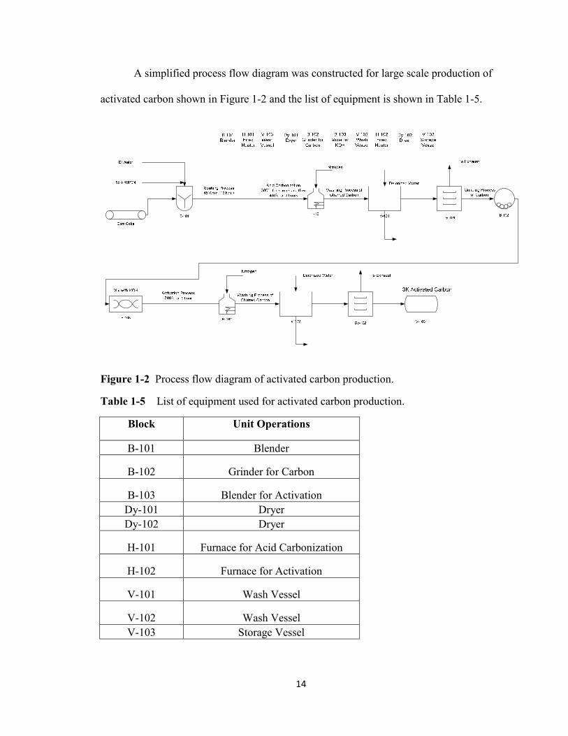
A simplified process flow diagram was constructed for large scale production of

activated carbon shown in Figure 1-2 and the list of equipment is shown in Table 1-5.

Figure 1-2 Process flow diagram of activated carbon production.

Table 1-5 List of equipment used for activated carbon production.

Block Unit Operations

B-101 Blender

B-102 Grinder for Carbon

B-103 Blender for Activation Dy-101 Dryer Dy-102 Dryer

H-101 Furnace for Acid Carbonization

H-102 Furnace for Activation

V-101 Wash Vessel

V-102 Wash Vessel V-103 Storage Vessel

15

The cost and size of equipment needed for producing 2000 lbs of activated carbon is

summarized in Table 1-6 using the CapCost 2008 program without recycle.

Table 1-6 Cost and size of equipment for carbon production without recycle.

Materials

Type Yearly Corn Cobs $ 2,480,000

H3PO4 $ 2,000,000

KOH $ 8,260,000

Total $12,740,000

Utilities

Type Yearly

Electricity $ 636,000 Natural

Gas $ 700,000

Blenders & Grinders

Unit Type Volume (ft3) Base Cost BMC

B-101 Rotary 1250.00 $ 236,000 $ 354,000

B-102 Rotary 618.00 $ 117,000 $ 176,000

B-103 Rotary 1020.00 $ 185,000 $ 278,000

Dryers

Unit Type Area (ft2) Base Cost BMC

Dy-101 Rotary 618.00 $ 268,000 $ 402,000

Dy-102 Rotary 306.00 $ 146,000 $ 219,000

Furnaces

Unit Type MOC Heat Duty (MJ/h) Base Cost BMC

H-101 Fired Heater CS 3210 $ 664,000 $ 1,410,000

H-102 Fired Heater CS 3610 $ 664,000 $ 1,410,000

Vessels

Unit Type MOC Diameter (ft) Length/Height (ft) Base Cost BMC

V-101 Horizontal Nickel 8.69 26.08 $ 37,000 $ 453,000

V-102 Horizontal CS 7.56 22.69 $ 28,100 $ 84,600

V-103 Horizontal CS 7.56 22.69 $ 28,100 $ 84,600

16

1.5.2.2. Annual Operating Costs

The annual utilities cost summary is shown in Table 1-7 broken down by

equipment type and form of utility used. Rough estimates (not recommended for design)

of the utilities were estimated as follows:

Table 1-7 Annual utilities cost summary of equipment used for carbon production.

Name Total Module Cost Grass Roots Cost Utility Used Efficiency

Actual Usage

Annual Utility Cost

B-101 $ 418,000 $ 536,000 NA

B-102 $ 208,000 $ 267,000 NA

B-103 $ 327,000 $ 420,000 NA

Dy-101 $ 474,000 $ 608,000 Electricity 2270 MJ/h $ 317,800

Dy-102 $ 258,000 $ 331,000 Electricity 2270 MJ/h $ 317,800

H-101 $ 1,670,000 $ 2,380,000 Natural

Gas 0.9 3570 MJ/h $ 329,500

H-102 $ 1,670,000 $ 2,380,000 Natural

Gas 0.9 4010 MJ/h $ 370,500

V-101 $ 534,000 $ 590,000 NA

V-102 $ 100,000 $ 142,000 NA

V-103 $ 100,000 $ 142,000 NA Totals $ 5,800,000 $ 7,800,000 $ 1,340,000

An equivalent annual operating cost was formulated in Table 1-8 using equations

found in Turton et al[19], taking into account capital cost, and estimated equipment life.

Table 1-8 Equivalent annual operating cost for carbon production.

Discount rate = 0.1

Equipment Capital Cost Operating Cost (per year)

Equipment Life (year)

Equivalent Annual Operating Cost (EAOC)

B-101 $ 536,000.00 $ 52,900.00 10 $ 140,000.00

B-102 $ 267,000.00 $ 52,900.00 10 $ 96,400.00

B-103 $ 420,000.00 $ 52,900.00 10 $ 121,000.00

H-101 $ 2,380,000.00 $ 329,500.00 10 $ 717,000.00

H-102 $ 2,380,000.00 $ 370,500.00 10 $ 758,000.00

Dy-101 $ 608,000.00 $ 317,800.00 10 $ 417,000.00

Dy-102 $ 331,000.00 $ 317,800.00 10 $ 372,000.00

V-101 $ 590,000.00 $ - 10 $ 96,000.00

V-102 $ 142,000.00 $ - 10 $ 23,100.00

17

V-103 $ 142,000.00 $ - 10 $ 23,100.00

Total EAOC= $ 2,760,000.00

*EAOC= (Capital investment)(A/P,I,neq) +(YOC)

The total summary of purchase costs is summarized in Table 1-9 broken down by

equipment type. The bare module cost is the summation of the bare equipment cost,

adjustment factors for design pressure, materials of construction, and equipment

setting[19]. And the grass roots cost refers to the cost of manufacturing the equipment

and building a completely new facility which is calculated by multiplying the bare

module cost by a factor of 1.68.

Table 1-9 Summary of total purchase costs of process equipment by equipment type.

Equipment Bare Module Cost Grass Roots Cost

Fired Heaters $ 2,820,000 $ 4,760,000

Blenders $ 808,000 $ 1,223,000

Dryers $ 621,000 $ 939,000

Vessels $ 622,200 $ 874,000

Total $ 4,870,000 $ 7,800,000 1.5.2.3. Net Present Value Over Ten Years

Taking into account the total initial investment needed for an annual production of

Activated Carbon, a net present value spreadsheet was created to analyze incoming and

outgoing cash flow, to appraise this project on a long term basis, and to provide an initial

foundation for capital budgeting[19]. The price of activated carbon calculated for a net

present value of zero during a period of ten years is shown in Table 1-10 below. The

initial investment includes the $7.8 million equipment cost with an additional ten percent

of the annual material cost, resulting in $9.85 million. The cost of manufacturing

18

includes the $12.7 million in raw material costs with utility costs, resulting in $14.04

million. The net present value calculation also incorporates a ten percent interest rate and

a 42% tax rate per year. The price of the carbon to break even in ten years is shown

below.

Table 1-10 Net Present Value calculations for the production of activated carbon (without recycle) in millions of dollars.

i(p.a.)= 0.1 WC(at the end of year 2)= 2.89

CL= 1.25 t= 0.42 /year

FCIL= 9.85 S= 0

5.5 year MACRS

End Of Year Investment R COMd Cashflow CCF dk

After-tax

Profit

After-tax Cash Flow

DCF DCCF

0 -9.85 0.00 0.00 -9.85 -9.85 0.00 0.00 -21.80 -21.80 -21.80

1 0.00 20.01 14.04 5.97 -3.88 1.97 2.32 4.29 3.90 -17.90

2 0.00 20.01 14.04 5.97 2.09 3.15 1.63 4.79 3.96 -13.94

3 0.00 20.01 14.04 5.97 8.06 1.89 2.37 4.26 3.20 -10.75

4 0.00 20.01 14.04 5.97 14.03 1.13 2.80 3.94 2.69 -8.06

5 0.00 20.01 14.04 5.97 20.00 1.13 2.80 3.94 2.45 -5.61

6 0.00 20.01 14.04 5.97 25.97 0.57 3.13 3.70 2.09 -3.52

7 0.00 20.01 14.04 5.97 31.94 0.00 3.46 3.46 1.78 -1.75

8 0.00 20.01 14.04 5.97 37.90 0.00 3.46 3.46 1.62 -0.13

9 0.00 20.01 14.04 5.97 43.87 0.00 3.46 3.46 1.47 1.34

10 1.25 20.01 14.04 7.22 51.09 0.00 3.46 -3.46 -1.33 0.00

NPV= 0.00

Rev/Year=

20.01 million

Carbon Produced = 2000 lbs/day

Carbon/year*= 700000 lbs/year

Cost of carbon needed to break even= $ 28.58 per lb

* Assumes 350 days/year for maintenance and holidays

1.5.2.4. Cost of Carbon Production with 70% Recycle

With an initial investment of $9.85 million and an annual cost of manufacturing

of $14.04 million which includes materials and utilities, an annual revenue of $20.01

19

million has to be generated, the cost of activated carbon is calculated to be $28.58 per

pound to break even over ten years. This price is considered to be noticeably higher

compared to commercial products, however, after a separate computation allowing for a

70% recycle of chemicals used provided by Aspen software, the materials and equipment

cost was dramatically decreased shown in Table 1-11.

Table 1-11 Cost and size of equipment for carbon production with 70% recycle.

Materials

Type Yearly

Corn Cobs $ 2,456,000

H3PO4 $ 590,000

KOH $ 2,497,000

Total $5,543,000

Utilities

Type Yearly

Electricity $ 60,820

Natural Gas $ 700,000

Blenders & Grinders

Unit Type Volume (ft3) Base Cost BMC

B-101 Rotary 26.68 $ 178,000 $ 266,000

G-101 Rotary 27.76 $ 181,000 $ 272,000

G-102 Rotary 22.24 $ 162,000 $ 242,000

Dryers

Unit Type Area (ft2) Base Cost BMC

Dy-101 Rotary 38.32 $ 28,300 $ 42,400

Dy-102 Rotary 17.55 $ 28,300 $ 42,400

Furnaces

Unit Type MOC Heat Duty (MJ/h) Base Cost BMC

H-101 Pyrolysis Nickel 3210 $ 462,000 $ 1,300,000

H-102 Activation Nickel 3610 $ 555,000 $ 1,560,000

Vessels

20

Unit Type MOC Diameter (ft) Length/Height (ft) Base Cost BMC

V-101 Horizontal Nickel Clad 8.16 24.47 $ 32,600 $ 228,000

V-102 Horizontal CS 7.51 22.57 $ 27,800 $ 83,600

V-103 Horizontal CS 8.11 24.32 $ 32,200 $ 96,800

1.6. Conclusion

Adsorbed natural gas technology provides a safe and environmentally friendly

alternative in fuel storage requiring simple compression, low pressure, and low

temperature surroundings. The production of extremely high porosity carbons have been

engineered for bulk storage natural gas vehicle applications.

The economics of activated carbon production relies heavily on product yield and

method of activation. Implementing a 70% recycle on the use of phosphoric acid and

potassium hydroxide plays a significant role in decreasing the price of carbon. These

economics are also considerably affected by selling the activated carbon in a price based

on its adsorption capacity and not on its weight[20] since its performance is substantially

better than commercial products currently in the market. Calculating the plant capacity at

its break-even point and conducting a sensitivity analysis would allow for future studies

in optimization and minimizing the cost of production to provide a greater incentive for

profit.

21

CHAPTER 2

INTRODUCTION OF BATTERY MODULE

2.1 Importance of Battery Technology and Introduction of Modules

The chemical engineering field of study is undergoing changes with goals of

introducing design earlier in the curriculum and increasing utilization of experiential

learning throughout the curriculum.[21] A modular battery experiment has been

developed and used in a sophomore-level mass and energy balance course and a junior-

level measurements lab toward these goals. These experiments assess the student’s

ability to use the techniques, skills, and modern engineering tools necessary for

engineering practice, and it also allows them to demonstrate their ability to design and

conduct experiments, and to analyze and interpret data.[22]

An additional goal of this module is to introduce chemical engineering students to

battery technology since batteries will play the pivotal role in energy security of modern

societies. As an alternative to petroleum, batteries can be used in hybrid electric vehicles

(HEVs) and plug-in HEVs to displace petroleum and increase the efficiency with which

limited petroleum resources are consumed. Alkaline manganese–zinc batteries are the

most convenient primary batteries as the source of power for portable electronic and

electric appliances.[23] For advanced devices, alkaline MnO2–Zn batteries are preferred,

which use electrolytic manganese dioxide (EMD) and an alkaline electrolyte (KOH).[24]

When used with the electric grid, batteries are able to enhance technologies related to

wind power, solar power, and peak load shifting.[25] These topics provide students with

22

exceptional platforms to which they can relate their investigations to contemporary

issues.

The battery- resistor circuit module allows heat transfer, mass transfer, reactions,

circuit theory, heat/mass balances, and product design to be studied in a single module.

The module also provides a good preparation for the study of sensors, biosensors, and

instrumentation because of its integrated approach using MATLAB, LabVIEW data

acquisition systems, and virtual instruments, which incorporates different aspects of the

engineering curriculum. Once the standardized workstations, stands, and storage are in

place, individual modules can be produced for a few hundred dollars with four modules

occupying about two square feet of space when stored in the storage cabinet.

The importance and utilization of battery technology has exponentially increased

in the last 20 years with the widespread introduction of hybrid electric vehicles (HEVs),

and society’s consciousness of using renewable resources and alternative energy. Due to

more rigorous environmental regulations, battery technology is a fundamental element to

initialize resource preservation efforts. Students will gain a practical laboratory

experience which incorporates theoretical modeling and real world applications of

batteries.

2.2 Objectives

• To develop experiments using the battery-resistor circuit module for the

University of Missouri – Department of Chemical Engineering within the Mass

and Energy Balance, Unit Operations, and Process Measurements courses

• To demonstrate fundamental concepts using modeling and simulations in a

battery-resistor circuit

23

• To introduce Laboratory Virtual Instrumentation Engineering Workbench

(LabVIEW) software and its integration with the undergraduate laboratory

modules

• To create Portable Document Format (PDF) files which demonstrate modular use

and software use for future students

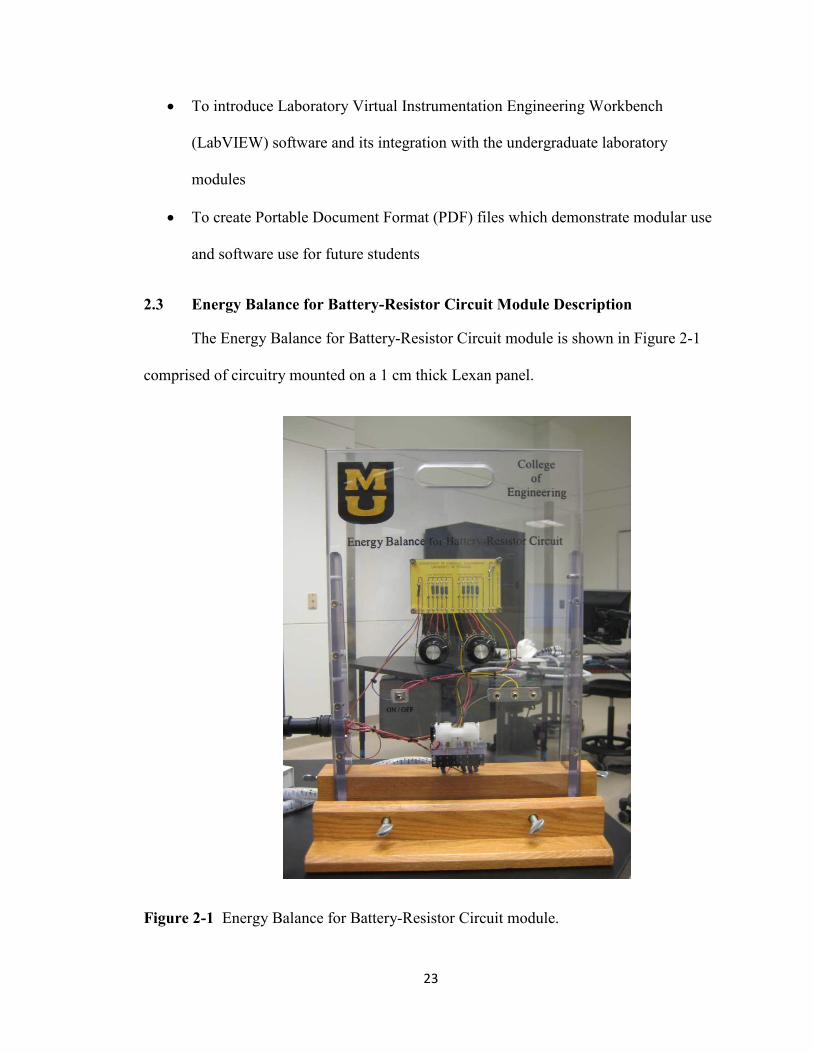
2.3 Energy Balance for Battery-Resistor Circuit Module Description

The Energy Balance for Battery-Resistor Circuit module is shown in Figure 2-1

comprised of circuitry mounted on a 1 cm thick Lexan panel.

Figure 2-1 Energy Balance for Battery-Resistor Circuit module.

24

The module consists of a resistor bank with several different settings and selector knobs

to control the total resistance applied to the battery, and switches to control where the

voltage is measured. The front panel also shows an AA battery holder that can also be

converted to connect to unconventional batteries made in the laboratory, and a data

acquisition cable connected to the module.

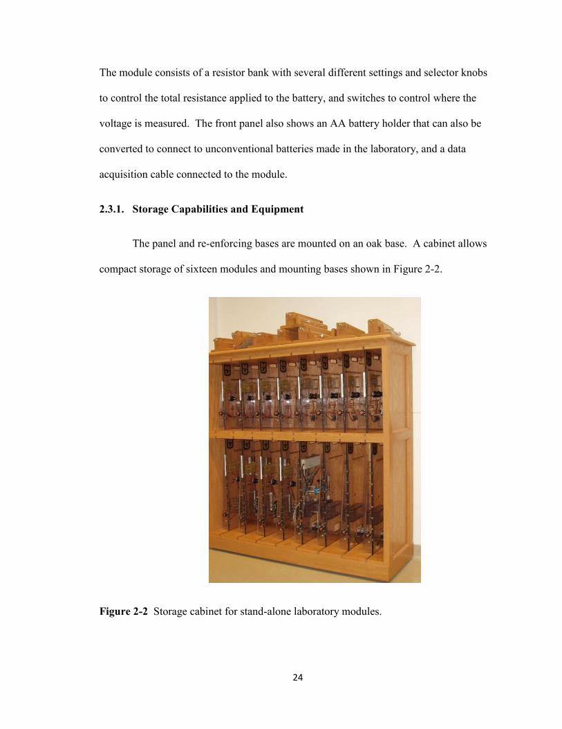
2.3.1. Storage Capabilities and Equipment

The panel and re-enforcing bases are mounted on an oak base. A cabinet allows

compact storage of sixteen modules and mounting bases shown in Figure 2-2.

Figure 2-2 Storage cabinet for stand-alone laboratory modules.

25

Each module connects to a computer workstation equipped with a National

Instruments data acquisition card: NI PCI-6259, a shielded connector block: NI SCB-68

and LabVIEW 8.6 software. Use of a standardized 24-pin connector allows different

experiments to use the same connector interface and respective workstation.

2.3.2. Description of Hardware and Circuitry

Figure 2-3 provides close up images of the AA battery connector, resistor bank,

and voltages switches. A small thermocouple embedded in the AA battery holder

monitors the battery temperature, which is used for the energy balance.

Figure 2-3 Close up images of module, including from left to right: AA battery holder; expanded image of 1-ohm resistor with thermocouple attached with shrink wrap; circuit board with 1-ohm resistor, two resistor banks, and knobs for selecting resistance from two resistor banks; and switches used to select locations for voltage measurements.

A second thermocouple is attached to the 1-ohm resistor—the temperature profile

of the 1-ohm resistor is the key measurement for the energy balance studies. The 1-ohm

resistor is connected in series with two other resistors from two resistor banks as selected

by the selector-switches. Each selector switch has five settings allowing 25 different

loads to be measured. The left selector switch has resistor settings 0, 1, 2, 3, and 5 ohms,

and the right selector switch has resistor settings 0, 5, 10, 20, and 30 ohms depicted by

26

Figure 2-4. These resistor banks allow variations in an assignment to be made so no two

groups or individuals have the same exact experiment. This allows the students to

compare their data with other individuals or groups to relate the effect of the changes in

resistor load, promoting a more interactive learning environment.[26]

2.3.3. Schematic of Resistor Bank

A series of three switches allow students to measure voltages at different locations

in the circuit. Figure 2-4 provides a schematic of the two resistor banks with the two

associated selector-switches, and the three switches that allow voltages to be measured

over the different loads. The first resistor bank consists of resistors 0, 1, 2, 3, and 5

ohms, and the second bank consists of resistors 0, 5, 10, 20, and 30 ohms.

Figure 2-4 Schematic of the experimental system which shows the different resistors in series and switch settings for voltage measurements.

Measure T AA

Battery

5 Ohm

30 Ohm

S1

3 Ohm

S2

20 Ohm

2 Ohm

10 Ohm

Measure T

1 Ohm

5 Ohm

0 Ohm

0 Ohm

S3

S4

S5

1 Ohm

VI

27

2.4 Data Acquisition Software

The LabVIEW program BatteryResistorEnergyBalance.VI is for the acquisition

of voltage profiles, and temperature profiles of the battery and 1-ohm resistor. LabVIEW

is installed on Dell workstation running on the Windows 7 operating system.

2.5 LabVIEW BatteryResistorEnergyBalance.VI Program Explanation

Figure 2-5 shows the front panel of the BatteryResistorEnergyBalance.VI

program which records voltage, resistor temperature, and battery temperature as a

function of time. Data files created by LabVIEW are readily accessible by MS Excel and

include columns of time, resistor temperature, battery temperature, and voltage (as

selected by the switch settings). The first time the experiment is run by a group, it takes

about 25 minutes. Subsequent runs take about 10-15 minutes.

Figure 2-5 Front panel view of LabVIEW BatteryResistorEnergyBalance.VI program.

28

The data display boxes on top of each graph show battery voltage in Volts, and

temperatures in degrees Celsius. The white “run” arrow at the top left of the screen will

prompt the user to indicate a location for the data file created by LabVIEW, and this will

also cause the program to initiate and start recording data.

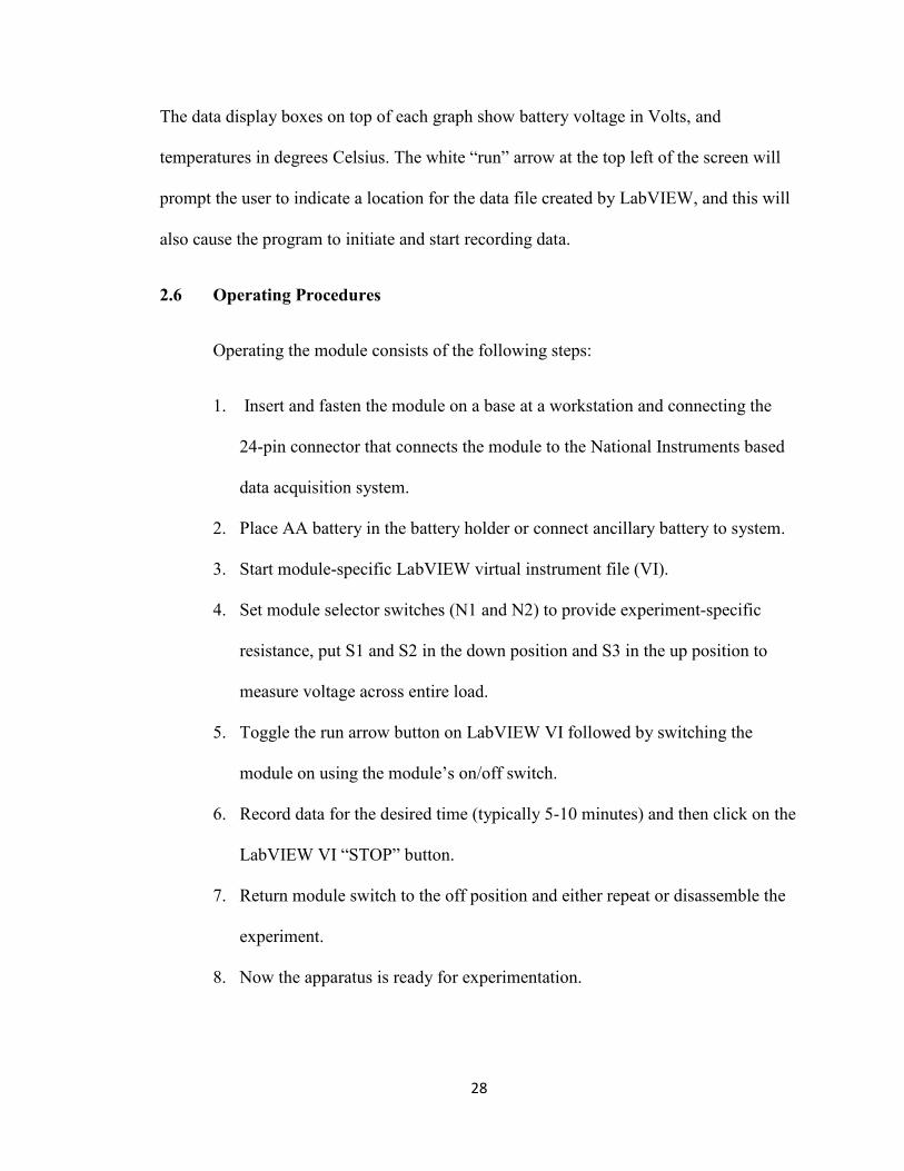
2.6 Operating Procedures

Operating the module consists of the following steps:

1. Insert and fasten the module on a base at a workstation and connecting the

24-pin connector that connects the module to the National Instruments based

data acquisition system.

2. Place AA battery in the battery holder or connect ancillary battery to system.

3. Start module-specific LabVIEW virtual instrument file (VI).

4. Set module selector switches (N1 and N2) to provide experiment-specific

resistance, put S1 and S2 in the down position and S3 in the up position to

measure voltage across entire load.

5. Toggle the run arrow button on LabVIEW VI followed by switching the

module on using the module’s on/off switch.

6. Record data for the desired time (typically 5-10 minutes) and then click on the

LabVIEW VI “STOP” button.

7. Return module switch to the off position and either repeat or disassemble the

experiment.

8. Now the apparatus is ready for experimentation.

29

CHAPTER 3

LABORATORY TEACHING MODULES

3.1 Introduction

These laboratory experiments can be used to develop fundamentals in engineering on

different educational levels in the undergraduate chemical engineering curriculum. The

students will apply practical skills such as modeling, simulations, and evaluations of a

dynamic model using both analytical and visual proficiencies. Three different

experiment-based projects can be performed using this module as follows:

• Battery Resistor Energy Balance

• Evaluating the Internal Resistance of a Battery

• Diffusion and Permeability in Manganese Dioxide-Zinc Battery

3.2 Project 1: Battery Resistor Energy Balance

The purpose of Mass and Energy Balance Experiment is to predict and then

model the transient temperature profile of the 1-ohm resistor that is connected in series

with two resistor banks and an AA battery. The students are also to develop applications

to measure and record temperature, voltage, current, and concentration of mass as a

function of time. Virtual instruments will be used to simulate different systems by the

use of various resistors and experimental data will be modeled as a function of time to

describe how the battery and resistor work in a circuit.

30

The students are given minimal guidance in the initial prediction of the

temperaure profile beyond a schematic of the circuit, knob settings, and the specification

of the brand name and type (zinc-alkaline) of battery.

Objectives:

• To use the Energy Balance for Battery-Resistor Circuit Module for applications

in the design of more efficient alkaline batteries

• To specify the design of the smallest alkaline battery capable of powering a 10W

light bulb for a period of one hour, using the same materials and chemistry as the

Duracell Procell Battery provided

• To understand how the battery and resistor function in a circuit over time, and to

extrapolate the information obtained to design a larger battery to power the light

bulb

• To perform simulations, preliminary and primary experimental measurements of

the system as well as modeling of the experimental data using Matlab and

different analytical approaches

3.2.1 Laboratory Operational Procedures

Procedure Set- Up Principle I. Operational Procedures

1. Obtain a circuit board and a base holder, noting the Module number

2. Insert the circuit board into the base and tighten the screws on the sides of the base holder first, and then loosely tighten the screws in front to prevent the glass from cracking

3. Make sure that the board is OFF before the battery is loaded, and insert the data

(It is best to use the same board for all data to decrease discrepancies) (This will make sure that the battery does not drain)

31

acquisition cable into the side of the board

II. Operational Procedures

1. The switch configurations should be S1 down, S2 down, and S3 up for this lab

2. Using the resistor dial, select the resistor needed for the experiment

3. Using the LabView software, open the BatteryResistanceEnergyBalance.vi

4. Run the program by clicking on the white arrow at the top left of the screen, and create a file name for your program

5. Turn on the circuit board (the LED light should come on)

6. Note any changes in battery voltage, resistor temperature, and battery temperature

7. To stop the program, click STOP to record the data, and THEN turn off the board to decrease discrepancies in the data

The S1 switch operates the thermocouple connected to the 1Ω resistor. The S2 switch controls the low resistance bank and the S3 switch operates the high resistance bank. Since the resistors are in series, they are added up across the board, but remember to include the 1Ω resistor attached to the thermocouple. The far left wire connected to the dial is the short circuit, resulting in 0 Ohms.

III. Maintenance a. The Module should be cooled for a

minimum of 30 minutes before performing the next experiment since temperature measurements are very sensitive

b. Be sure to disassemble the data acquisition cable, circuit board, and base holder and put away the materials when you leave

32

3.2.2. Governing Differential Equations

The students are responsible for the derivation of governing differential equations

such as the equation for change in resistor temperature as a function of time,

which

can be derived from the change in internal energy over time;

.[27] The students are to

identify how voltage drop and amperage translate to a heat input term in a first law

balance, and they are to estimate parameters such as heat capacity and mass. They are

encouraged to use MatLab to solve the differential equations that govern the system.

The following are pertinent governing equations:

(3-1)

(3-2)

(3-3)

3.2.3. Modeling Data

During initial predictions the students will typically neglect the convective cooling

of the resistor by ambient air or they will struggle to identify how to model the heat

transfer. Most students have not had a course in heat transfer, and when they identify the

need to apply an engineering science that they have not yet covered they are directed to

research the use of heat transfer coefficients.[28] The need to take into account the

convective heat transfer term to model the temperature profile of the resistor will become

evident when they obtain experimental temperature profiles. If convection was not

identified during the predictive modeling stage of the project, the temperature profile

indicates the need to modify the model battery. Figure 3-1 shows the raw experiemental

33

data, and Figure 3-2 depicts the superimposed model after is is fitted with the experiental

data. The modeling process provides a conceptual learning element because the students

can visually relate how changing the heat transfer coefficients modifies the temperature

profile.[22]

Figure 3-1 A plot of the resistor and battery temperature profile with a 3 Ohm total resistor.

Some of the modeling parameters are shown in Table 3-1 including heat transfer

coefficients, heat capacity, total resistance applied to the battery, time span required to run

the experiment, and initial temperature. These parameters are inputed into various

MATLAB codes to model and plot the data.

Table 3-1 Sample parameters used model the resistor temperature versus time.

Model Parameters used for the Resistor Temperature vs. Time

mC 1.675

hA .255

R 3

Tspan [1, 289]

To 20.95

0 200 400 600 800 1000 120020

22

24

26

28

30

32

34

36

38

40

Time (s)

Temperature (C)

Preliminary Experimental Measurements (3 Ohm)

ResistorBattery

34

Figure 3-2 provides a typcial resistor temperature versus time profile with

modeling results and a voltage profile for battery discharge operating with a 3-ohm total

resistance load.

Figure 3-2 A plot of the resistor temperature with superimposition of modeling results (left) and voltage profile of the battery operating with a 3 Ohm total resistor (right).

The resistor temperature versus time profile can be used to model the resistor temperature

as a function of time by manipulating hA, the heat transfer coefficient, and mC, the heat

capacity, in the MATLAB program. The decreasing temperature is a manifestation of

decreasing voltage power output from the AA battery which is under a heavy load.[29]

This aspect of the project introduces the challenge of how to handle the modeling of the

resistor temperature for a non-constant voltage term—this introduces the utility for

numerical solution of ordinary differential equations when analytical solutions may not

be an option.[30]

The voltage data shown in Figure 3-2 behaved accordingly to theory because

there is a rapid decrease at first because a battery can only perform at its ideal for a short

amount of time. The steep drop in voltage at the beginning of the plot is due to the power

supply being turned on at the start of the experiment after the run has already begun. The

voltage then gradually decreases as a slower rate as the time increases.

0 200 400 600 800 1000 120020

22

24

26

28

30

32

34

36

38

40

Time [s]

Resistor Tem

perature [C]

ModelExperimental Data

0 200 400 600 800 1000 12001.25

1.3

1.35

1.4

1.45

1.5

1.55

1.6

Time (s)

Voltage (V)

Voltage

35

Another aspect of this lab can be used to measure battery efficiency by measuring

actual voltage, shown in Figure 3-2, delivered by the battery divided by the ideal voltage.

The students will be able to follow the temperature profile of the battery and visually

understand and verify what happens to the lost energy.[31]

3.2.4. Other Applications

For semester-long projects, the students are able to sequentially perform the following:

1. Convert the voltage profile of Figure 3-2 to battery efficiency versus time.

2. Obtain battery voltages at a specified times (e.g. 30 seconds into discharge)

over multiple resistances then use these data to prepare a battery performance

curve (Voltage versus Amperage).

3. Fully deplete a battery to obtain the amp-hours of energy the battery is able to

deliver and compare this to the mass of the battery components (as estimated

based on Material Safety Data Sheet (MSDS) information).

4. Use the performance curve (from 2), amount of active reagent utilization

(from 3), membrane surface area (membrane that separate cathode from

anode, an estimated value) to design a battery for a different application (e.g.

powering a 20 W light bulb for 2 hours).

A project based on these steps provides a valuable experiential leaning process

involving: energy balances, transient energy balances, basic circuit theory, modeling

versus predictive simulation, convective heat transfer, analytical versus numerical

solution methods, mass balances, transient mass balances, battery performance curves,

and product design.[32]

36

3.2.5. Sample Outline for Project 1: Battery Resistor Energy Balance

Project Objective

The purpose of this lab is to develop applications to measure and record

temperature, voltage, current, and concentration of mass as a function of time. Virtual

instruments will be used to simulate different systems by the use of various resistors and

experimental data will be modeled as a function of time to describe how the battery and

resistor work in a circuit.

Part A

Given project-specific settings for S1 and S2 (this is given), estimate the temperature

of the 1 Ohm resistor when the circuit is closed based on initial conditions at ambient

temperature. Perform a-e in this analysis. How long will it take for a temperature

rise of 4°C?

a. Derivation of governing differential equations.

o Derive the equation for change in resistor temperature as a function of

time,

and include this in your report

b. Simulation of system using analytical approaches a possible and using Matlab

(including temperature increase). Each person will be given a specific

resistance at which to model the resistor and the battery.

o Use Matlab to define and solve the differential equation, and to import

and plot the data

c. Primary experimental measurements on the system.

o Use project specific settings for S1 and S2

37

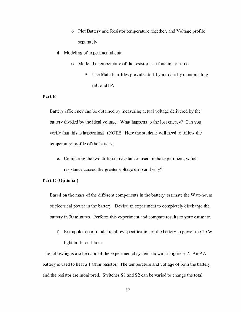
o Plot Battery and Resistor temperature together, and Voltage profile

separately

d. Modeling of experimental data

o Model the temperature of the resistor as a function of time

§ Use Matlab m-files provided to fit your data by manipulating

mC and hA

Part B

Battery efficiency can be obtained by measuring actual voltage delivered by the

battery divided by the ideal voltage. What happens to the lost energy? Can you

verify that this is happening? (NOTE: Here the students will need to follow the

temperature profile of the battery.

e. Comparing the two different resistances used in the experiment, which

resistance caused the greater voltage drop and why?

Part C (Optional)

Based on the mass of the different components in the battery, estimate the Watt-hours

of electrical power in the battery. Devise an experiment to completely discharge the

battery in 30 minutes. Perform this experiment and compare results to your estimate.

f. Extrapolation of model to allow specification of the battery to power the 10 W

light bulb for 1 hour.

The following is a schematic of the experimental system shown in Figure 3-2. An AA

battery is used to heat a 1 Ohm resistor. The temperature and voltage of both the battery

and the resistor are monitored. Switches S1 and S2 can be varied to change the total

38

resistance of the circuit to allow additional data to be obtained and/or to allow different

groups to have different project definitions while using the same experimental system.

Figure 3-3 Schematic of resistor bank on module.

Measure TAA Battery

5 Ohm 30 Ohm

S1 3 Ohm S2 20 Ohm

2 Ohm 10 Ohm

Measure T 1 Ohm 5 Ohm

0 Ohm 0 Ohm

S3 S4 S5

1 Ohm

VI

39

3.2.6. MatLAB Codes for Project 1: Battery Resistor Energy Balance

Data Import

uiimport Time=data(:,1); ResistorTemp=data(:,2); BatteryTemp=data(:,3); Voltage=data(:,4); plot(Time, ResistorTemp) hold all plot(Time, BatteryTemp) hold off plot(Time, Voltage)

MEB Data Extraction

Time = data(:,1); %Takes all values in first column of "data" array and gives it the name "Time" ResistorTemp = data(:,2); %Takes all values in second column of "data" array and gives it the name "ResistorTemp" BatteryTemp = data(:,3); % Takes all values in third column of "data" array and gives it the name "BatteryTemp" Voltage = data(:,4); % Takes all values in forth column of "data" array and gives it the name "Voltage" InitialTime = Time(1,1) %Gives the initial time value FinalTime = Time (289,1) %Gives the last time value...by looking at the "workspace" tab my "data" array has a value of <1676x4 double> this means the array has 1676 lines and 4 columns, so my "Time" array will have 1676 values and #1676 will be my final time InitialTemp = ResistorTemp(1,1) ) %Gives initial temperature to use as initial condition in the differential equation

Dual Plot Solver

solver %Use the name of ODE solver m-file you created previously hold on %Allows for multiple plots to be displayed on same figure plot(Time- InitialTime,ResistorTemp)%Plots ResistorTemp as a function ot Time hold off %Stops allowing plots to be added to same figure

%Adds axis titles and a legend to the figure xlabel('Time [s]'); ylabel('Resistor Temperature [C]'); legend('Model','Experimental Data','Location','South');

40

Solver

tspan=[InitialTime FinalTime]; T0=InitialTemp; [t,T] = ode45(@difftemp, tspan, T0); plot(t-InitialTime,T,'Color','red');

To Model Data

function Tprime = difftemp(t,T,mC,hA,P,R,Tamb); mC=1.675; hA=0.255; P=0.05291*exp(-0.0009862*t)+0.1703*exp(-2.636e-5*t); R=3; Tamb=20.95; Tprime = ((1/mC)*P)-((hA/mC)*T)+((hA/mC)*Tamb);

41

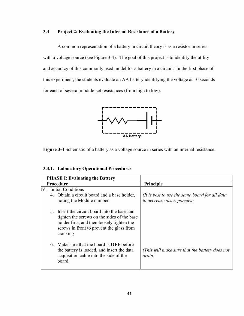
3.3 Project 2: Evaluating the Internal Resistance of a Battery

A common representation of a battery in circuit theory is as a resistor in series

with a voltage source (see Figure 3-4). The goal of this project is to identify the utility

and accuracy of this commonly used model for a battery in a circuit. In the first phase of

this experiment, the students evaluate an AA battery identifying the voltage at 10 seconds

for each of several module-set resistances (from high to low).

Figure 3-4 Schematic of a battery as a voltage source in series with an internal resistance.

3.3.1. Laboratory Operational Procedures

PHASE I: Evaluating the Battery Procedure Principle

IV. Initial Conditions 4. Obtain a circuit board and a base holder,

noting the Module number

5. Insert the circuit board into the base and tighten the screws on the sides of the base holder first, and then loosely tighten the screws in front to prevent the glass from cracking

6. Make sure that the board is OFF before the battery is loaded, and insert the data acquisition cable into the side of the board

(It is best to use the same board for all data to decrease discrepancies) (This will make sure that the battery does not drain)

AA Battery

42

V. Operational Procedures

8. The switch configurations should be S1 down, S2 down, and S3 up for this lab

9. Using the resistor dial, select the resistor needed for the experiment

10. Using the LabView software, open the BatteryResistanceEnergyBalance.vi

11. Run the program by clicking on the white arrow at the top left of the screen, and create a file name for your program

12. Turn on the circuit board (the LED light should come on)

13. Note any changes in battery voltage, resistor temperature, and battery temperature

14. To stop the program, click STOP to record the data, and THEN turn off the board to decrease discrepancies in the data

The S1 switch operates the thermocouple connected to the 1Ω resistor. The S2 switch controls the low resistance bank and the S3 switch operates the high resistance bank. Since the resistors are in series, they are added up across the board, but remember to include the 1Ω resistor attached to the thermocouple. The far left wire connected to the dial is the short circuit, resulting in 0 Ohms.

Analysis of the data for this project can be obtained by linear regression of an

equation derived as follows.[33] Where:

o= I (RBattery + RCircuit) (3-4)

The current (I) for each experiment can be identified by this same equation

evaluated over the circuit load rather than the theoretical voltage of the battery:

= VCircuit / RCircuit (3-5)

Or

Circuit = Vo - RBattery(VCircuit / RCircuit) (3-6)

Where linear regression can be used to identify VO (constant) and RBattery (slope).

43

Figure 3-5 Example results from PROJECT 2 and equation 3-6 for evaluating the internal resistance of a battery. The data are for different circuit resistances evaluated with the experimental module.

Figure 3-5 illustrates experimental data plotted according to equation 3-6 with an

excellent correlation and little scatter. The students are expected to analyze their data and

understand why the internal resistance of the battery stays constant, using equations to

justify their results. The internal resistance of the battery is relatively constant for data

taken at a constant time of exposure to a load. For low resistances, the resistance of the

battery will decrease with time due to increased diffusion over-potential as the substrates

closest to the membrane are consumed.[34] This trend is seen for the right-most data

point, and for this reason, the linear regression was performed without including that data

point.

Extensions of this project could include evaluating the internal battery resistance

at different times the battery is under load.[35] Detailed discussions related to transient

diffusions in packed-bed anodes could be used to explain the dependence of the internal

battery resistance on time. If the students are able to do the sophisticated modeling, the

1.220

1.240

1.260

1.280

1.300

1.320

1.340

1.360

1.380

0 0.1 0.2 0.3 0.4 0.5

Vc

(Vol

ts)

Vc / Rc (Amps)

Vo

Slope = - RBattery

44

diffusion in the packed bed could be modeled, converted to diffusion over-potential, and

interpreted in terms of a resistor model.

3.2. Sample Outline for Project 2

Project Outline: Evaluating the Internal Resistance of a Battery

Phase 1 – A common representation of a battery for circuit representation purposes is as

a resistor in series with a voltage sources (see Figure 3-6). In the first phase of this

experiment, you are to evaluate an AA battery for about 10 seconds at each of several

module-set resistances (from high to low) to evaluate if this model of a battery is

accurate. The experimental component of this phase should take about 5 minutes.

Figure 3-6. Model illustration of a battery as a

voltage source in series with an internal resistance.

a. Run the module for 10 seconds, and note the open- circuit voltage and the voltage

at the 10 second interval. Use this information to find the internal resistance

of the battery (RB) of each resistance and compare them to each other.

i. Open a new file each run, and use the following total resistances to

run your module: 3Ω, 6Ω, 11Ω, 16Ω, 26Ω, 36Ω

3.4 Project 3: Diffusion and Permeability in a Manganese Dioxide-Zinc Battery

AA Battery

The objective of this project is to evaluate batteries that the students assemble.

The students are also to relate fundamental differences of the battery performances to

properties of the materials and the cell geometry, and to quantitatively correlate the

performance to diffusivity resulting from varying the separator material. The use

zinc electrode anode is important because of its high open

electrolyte, a low corrosion rate, and a low material cost.

A schematic of the battery as

packing, cathode packing, separator materials, and premixed electrolyte are provided to

the students for assembling the batteries. The electrode packings are volumetrically

dispensed into the cell being separated by the separator materia

used to connect the current collectors of the battery assembly to the AA battery holder

points of contact on the experimental module.

Figure 3-7 Pictorial representation of a compression cell used for the assembly of MnO– Zn batteries (left) with picture of assembled cell (middle) and an assembled cell with weight to provide compression (right).

The experimental procedures include assembling several Zn

different separator materials and evaluate the perf

powder is used as the anode packing in preference to zinc foil or plates because of its 45

The objective of this project is to evaluate batteries that the students assemble.

he students are also to relate fundamental differences of the battery performances to

properties of the materials and the cell geometry, and to quantitatively correlate the

performance to diffusivity resulting from varying the separator material. The use

zinc electrode anode is important because of its high open-circuit voltage in the KOH

electrolyte, a low corrosion rate, and a low material cost.[36]

A schematic of the battery assembly is provided by Figure 3-7. Prepared anode

packing, cathode packing, separator materials, and premixed electrolyte are provided to

the students for assembling the batteries. The electrode packings are volumetrically

dispensed into the cell being separated by the separator materials. Alligator clips are

used to connect the current collectors of the battery assembly to the AA battery holder

points of contact on the experimental module.

Pictorial representation of a compression cell used for the assembly of MnOZn batteries (left) with picture of assembled cell (middle) and an assembled cell with

weight to provide compression (right).

The experimental procedures include assembling several Zn-MnO

different separator materials and evaluate the performance in a 33- ohm circuit. Zinc

powder is used as the anode packing in preference to zinc foil or plates because of its

The objective of this project is to evaluate batteries that the students assemble.

he students are also to relate fundamental differences of the battery performances to

properties of the materials and the cell geometry, and to quantitatively correlate the

performance to diffusivity resulting from varying the separator material. The use of a

circuit voltage in the KOH

. Prepared anode

packing, cathode packing, separator materials, and premixed electrolyte are provided to

the students for assembling the batteries. The electrode packings are volumetrically

ls. Alligator clips are

used to connect the current collectors of the battery assembly to the AA battery holder

Pictorial representation of a compression cell used for the assembly of MnO2

Zn batteries (left) with picture of assembled cell (middle) and an assembled cell with

MnO2 batteries with

ohm circuit. Zinc

powder is used as the anode packing in preference to zinc foil or plates because of its

46

large surface area to distribute solid and liquid phases more homogeneously.[37] A high

zinc surface area to volume ratio is needed for high-rate capability and zinc oxide will

form on the surface of the zinc as summarized by the following half reactions:[38]

Zn (s) + 2OH− (aq) → ZnO (s) + H2O (l) + 2e− (3-7)

2MnO2 (s) + H2O (l) + 2e− →Mn2O3 (s) + 2OH− (aq) (3-8)

Manganese oxide powder mixed with a carbon black is used as the cathode. The

carbon is used to increase conductivity of the positive active mass to reduce the internal

resistance of the cell.[39] This material may require mechanical processing to maximize

reactivity.[40] Potassium hydroxide (1M or 2M) in distilled water works well as the

electrolyte because of its high conductivity, and results in a low internal resistance.[41]

In the presence of KOH, the discharge behavior of MnO2 occurs in a heterogeneous

phase reaction.[42]

3.4.1. Laboratory Operational Procedures

Phase II: Battery Assembly of Zn- MnO2

Procedure Principle

***EYE PROTECTION AND GLOVES REQUIRED*** VI. Operating Procedures

a. Obtain a Compression Cell and a 6Kg weight

b. In the glove box, start to assemble the battery by inserting the base of the compression cell first ( the shorter piston)

c. Place ~0.15g of the cathode material (!"#) into the cylinder (enough to cover a thin layer on the bottom of the cell) and tap the cell to create an even distribution

Keep in mind which side of the compression cell the anode or cathode material is being placed. This is important when connecting the positive and negative leads Use the spatula to flatten out the filter paper and tap out the excess cathode material

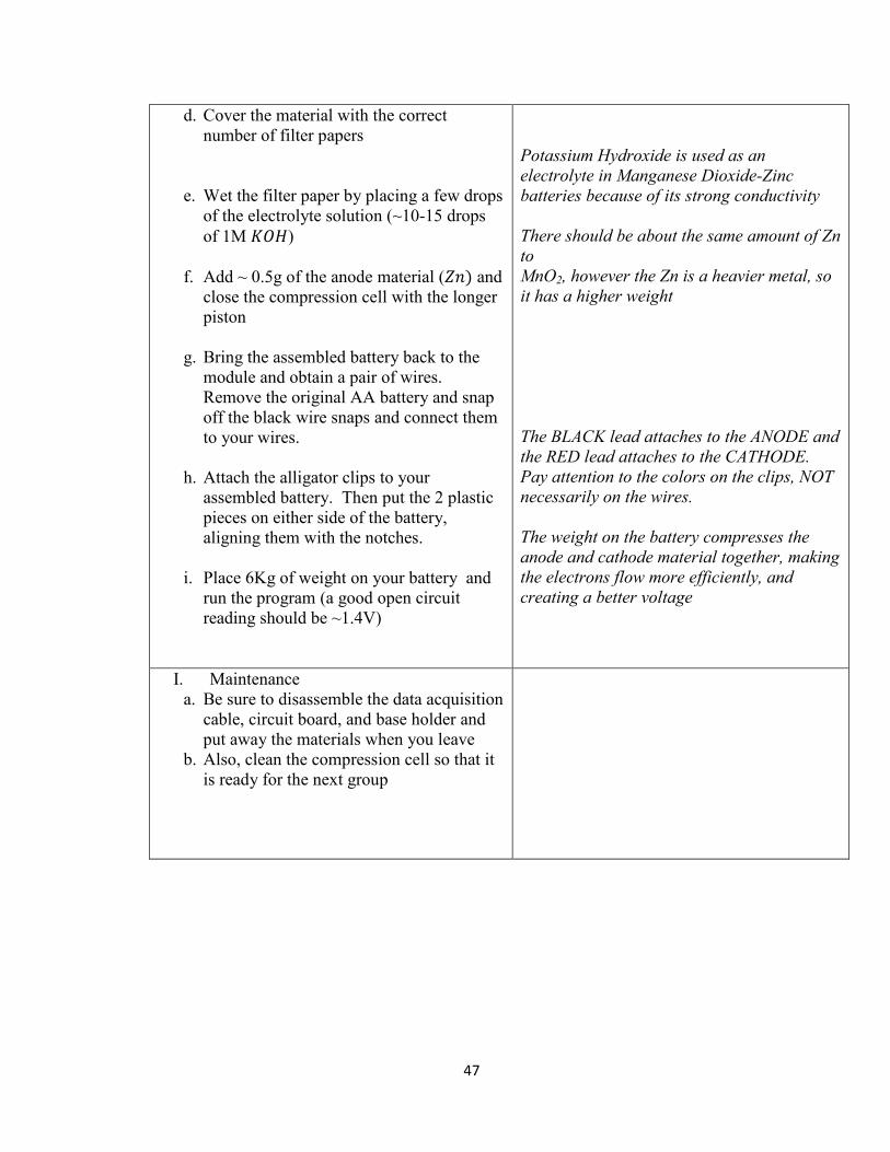
47

d. Cover the material with the correct number of filter papers

e. Wet the filter paper by placing a few drops of the electrolyte solution (~10-15 drops of 1M $#%)

f. Add ~ 0.5g of the anode material (&" and

close the compression cell with the longer piston

g. Bring the assembled battery back to the

module and obtain a pair of wires. Remove the original AA battery and snap off the black wire snaps and connect them to your wires.

h. Attach the alligator clips to your

assembled battery. Then put the 2 plastic pieces on either side of the battery, aligning them with the notches.

i. Place 6Kg of weight on your battery and

run the program (a good open circuit reading should be ~1.4V)

Potassium Hydroxide is used as an electrolyte in Manganese Dioxide-Zinc batteries because of its strong conductivity There should be about the same amount of Zn to MnO2, however the Zn is a heavier metal, so it has a higher weight The BLACK lead attaches to the ANODE and the RED lead attaches to the CATHODE. Pay attention to the colors on the clips, NOT necessarily on the wires. The weight on the battery compresses the anode and cathode material together, making the electrons flow more efficiently, and creating a better voltage

I. Maintenance a. Be sure to disassemble the data acquisition

cable, circuit board, and base holder and put away the materials when you leave

b. Also, clean the compression cell so that it is ready for the next group

48

3.4.2. Separator Material for Cathode and Anode

The separator materials provide the best opportunity to systematically vary a

parameter that impacts battery performance. Sheets of permeable material can be

punched to sizes that match the inner diameter of the battery’s polyethylene sleeve.

When preparing the battery, care must be taken to assure that the permeable separator

totally separates the anode from the cathode or the battery will short circuit. Filter paper

work well as separators with the experimental parameter being the number of sheets of

filter paper placed between the anode and cathode. The filter paper used in this

experiment is a qualitative type with course porosity and a fast flow rate from Fisher

Brand. More sheets will create greater resistance to diffusion and greater over-potential

losses.[34] It is also beneficial to have a negative control of a non-permeable

polypropylene membrane to confirm that in the absence of a diffusive path between the

anode and cathode, the battery voltage will immediately go to zero.

The test cell (Figure 3-7) is basically a compression cell comprised of two pistons

inside a non-conductive sleeve. The battery is assembled by inserting the base of the

compression cell first (the shorter piston). It is assembled as follows:

1. Place a volumetrically dispersed amount of the cathode material (!"#) into the

cylinder (enough to cover a thin layer on the bottom of the cell) and tap the cell to

create an even distribution.

2. Cover the material with the correct number of filter papers (qualitative P8 Fisher

Brand).

49

3. Wet the filter paper by placing a few drops of the electrolyte solution (~10-15

drops of 1M$#%). Potassium Hydroxide is used as an electrolyte in Manganese

Dioxide-Zinc batteries because of its strong conductivity.

4. Add a thin layer of the anode material (&" and close the compression cell with

the longer piston.

5. Bring the assembled battery back to the module and obtain a pair of wires.

Remove the original AA battery, snap off the battery power adapters and connect

them to the wires.

6. Attach the alligator clips to the assembled battery and put the two plastic pieces

on the top and bottom of the assembled battery, aligning them with the notches.

7. Place a 6 kg weight on the assembled battery and run the program. The weight on

the battery compresses the anode and cathode material together, making the

electrons flow more efficiently, and creates a better voltage.[43]

3.4.3. Diffusivity and Permeability Results

Figure 3-8 summarizes representative data for a study of 2, 4, and 6 layers of filter

paper, and a negative control using polypropylene as a non-permeable membrane

separating the anode material from the cathode material keeping the time of the

experimental runs constant. The polypropylene membranes used in this experiment were

obtained using the same hole-punch technique as the filter papers, using a petri-dish as

the material. Battery performance typically consists of a steep drop in voltage initially

and then a steady decline. At a constant load, an increase in resistance (more layers of

filter paper) results in a lower voltage delivered to the resistor.[34] Ideally, the voltage

for the non-permeable membrane should immediately drop to zero, however, because of

50

the difficulties involved in constructing a perfect separation seal, there may be some

voltage detected due to the seepage and mixing of the anodic and cathodic material

around the outer perimeter of the polypropylene membrane.

Figure 3-8 Graph of results showing proposed trend of decreasing voltage with increasing resistance of separator between electrodes. The numbers indicate the number of layers of filter paper between the electrodes.

The students should be able to qualitatively understand how increased diffusion

distances through permeable materials translate to increased voltage over-potentials.[34]

In more advanced applications, the permeability can be related to voltage. Other

variations from this experiment include use of battery assemblies with different inner

diameters and use of non-permeable separators cut into washer-shapes that vary the

cross-sectional area available for diffusion.

3.4.4. Sample Outline for Project 3

Project Outline: Diffusivity and Permeability in a Manganese Dioxide- Zinc Battery

Phase 2 –You are to assemble several Zn-MnO2 batteries with different materials

(specified in group project specification) separating the anode from the cathode. The

0

0.2

0.4

0.6

0.8

1

1.2

1.4

1.6

0 50 100 150 200 250

Volt

age

(V)

Time (s)

2 Filter Paper

4

6Negative Control

51

assembled battery will be connected to the module via wire leads. We will run the total

resistance of the battery at 33 Ohms. Use Figure 3-9 as a schematic for the resistor bank

for reference.

a. Each group will assemble their battery with a negative control, 2, 4, and 6 filter

papers separating the anode material from the cathode material to witness the

ion’s diffusivity and to notice a trend regarding voltage, current, and the layers of

filters with respect to time.

a. The negative control will be used with a polypropylene non-permeable

membrane.

b. Run the LabVIEW program using the assembled battery; you will notice a steep

drop in voltage initially and then a steady decline. A good Zinc battery should

have about 1.4V at open circuit. Stop the program at 2 minutes. And then, turn

the module OFF.

c. Using MatLAB, import the files and define your variables using this code in the

command prompt:

uiimport Time=data(:,1); ResistorTemp=data(:,2); BatteryTemp=data(:,3); Voltage= data(:,4); plot(Time, Voltage) I= Voltage./(Total Resistance)

i. When you import your data, cut out the voltage data in open circuit

using the header function

ii. The Total Resistance should be the resistance that was assigned

earlier. This gives an equation for Current.

52

iii. The use the function trapz(Time, I) in the command line to

integrate the current to obtain Coulombs. Then divide by Faraday’s

constant to obtain moles of electrons.

d. Plot all 4 experimental runs on the same graph with respect to time. Make 2

separate graphs: Voltage vs. Time, and Current vs. Time

e. Evaluate the diffusivity of the battery if there is a consistent trend. Relate the flow

of ions through the electrolyte solution to the thickness of the filters separating the

cathode and anode material. Use the mass flux equation and Fick’s law of

diffusivity to support your answer.

f. Calculate the total power output of each experimental run by integrating Power/

Time and discuss your results.

Objective - The objective is to relate fundamental differences of the battery

performances to thermodynamic properties of the materials and the cell geometry, and to

quantitatively relate the performance to diffusivity (or apparent diffusivity/permeability)

of your separator material.

Figure 3-9 Schematic of resistor bank.

AA Battery

5 Ohm 30 Ohm

S1 3 Ohm S2 20 Ohm

2 Ohm 10 Ohm

Measure T 1 Ohm 5 Ohm

0 Ohm 0 Ohm

S3 S4 S5

1 Ohm

VI

53

3.5 Student Feedback

For Project 1, the students recognized and appreciated how energy is converted

from chemical to thermal forms and how transient differential models can relate

underlying engineering science (ohms law, convective heat transfer) to observed

phenomena. The most frequent problem encountered was a lack of attention by the

students on which voltages were actually being measured during the experiment. Project

2 was a simple and straight forward experiment that validates a commonly used model

for batteries. Students that expected the need for a detailed analysis based on differential

equations were disappointed. Project 3 was effective in getting students to contemplate

some more complicated aspects of mass transfer and how mass transfer limits the

performance of a battery. The primary concern with Project 3 was that sloppy

preparation of the assembled battery could result in inconsistent data.

3.6 Conclusion

The battery provides an excellent basis for student projects in chemical

engineering. The module described in this paper provides a way to delivery experiential

learning with batteries in open formats that can be used with a variety of lecture-based

courses. The students are able to directly connect with what they observe in the

experiential learning because they encounter and frequently use batteries in their day-to-

day routines. Different variations of battery-based projects allow students to use energy

balances, transient energy balances, basic circuit theory, modeling versus predictive

simulation, convective heat transfer, analytical versus numerical solution methods, mass

balances, transient mass balances, battery performance curves, and product design.

54

REFERENCES [1] C. U. Ikoku, Natural Gas Engineering. Tulsa, Oklahoma: PennWell Publishing

Company, 1980. [2] M. Kelkar, Natural Gas Production Engineering. Tulsa, Oklahoma: PennWell

Corporation, 2008. [3] "How Safe Are Natural Gas Vehicles?," Clean Vehicle Education Foundation, p. 3, 2010. [4] P. S. Shah, "Nanoporous Carbon from Corn Cobs and its Applications," PhD, Chemical

Engineering, University of Missouri, Columbia, 2007. [5] H. Najibi, et al., "Methane/Natural Gas Storage and Delivered Capacity for Activated

Carbons in Dry and Wet Conditions," Fuel, vol. 87, pp. 7-13, 2007. [6] N. Bagheri and J. Abedi, "Preparation of High Surface Area Activated Carbon From

Corn By Chemical Activation Using Potassium Hydroxide," Chemical Engineering Research and Design, vol. 87, pp. 1059-1064, 2009.

[7] E. Salehi, et al., "Theoretical and Experimental Study on the Adsorption and Desorption of Methane by Granular Activated Carbon at 25C," Journal of Natural Gas Chemistry, vol. 16, pp. 415-422, 2007.

[8] M. J. Prauchner and F. R.-. Reinoso, "Preparation of Granular Activated Carbons for Adsorption of Natural Gas," Microporous and Mesoporous Materials, vol. 109, pp. 581-584, 2008.

[9] R. C. Bansal and M. Goyal, Activated Carbon Adsorption. Boca Raton, FL: CRC Press Taylor & Francis Group 2005.

[10] R. W. Judd, et al., "The Use of Adsorbed Natural Gas Technology for Large Scale Storage," American Chemical Society Division of Fuel Chemistry, p. 575, 1998.

[11] H. Jankowska, et al., Active Carbon. Warsaw, Poland: Ellis Horwood Limited Wydawnictwa Naukowo-Techniczne, 1991. [12] M. Molina-Sabio, et al., "Phosphoric Acid Activated Carbon Discs for Methane

Adsorption," Carbon, vol. 41, pp. 2113-2119, 2003. [13] J. W. Hassler, Activated Carbon. New York: Chemical Publishing Co.,Inc. , 1963. [14] D. Quinn, "Adsorption Storage: A Viable Alternative to Compression for Natural Gas

Powered Vehicles," ed. Royal Military College of Canada, 2006. [15] T. J. Bandosz, Activated Carbon Surfaces in Environmental Remediation. New York:

Elsevier, 2006. [16] U. N. A. S. Service, "Missouri State Agriculture Overview," M. A. Overview, Ed., ed,

2009. [17] E. Liemkuehler, "Production, Characterization, and Applications of Activated Carbon,"

MS, Chemical Engineering, University of Missouri, Columbia, 2010. [18] H. Marsh and F. R. Reinoso, Activated Carbon. Amsterdam: Elsevier Science and

Technology, 2006. [19] R. Turton, et al., Analysis, Synthesis, and Design of Chemical Processes, Third Edition.

Boston: Prentice Hall, 2009. [20] G. G. Stavropoulos and A. A. Zabaniotou, "Minimizing Activated Carbons Production

Cost," Fuel Processing Technology, vol. 90, p. 952, 2009. [21] A. Rugarcia, et al., "Future of Engineering Education. I. A Vision for a New Century,"

Chemical Engineering Education [22] R. M. Felder and R. Brent, "Designing and Teaching Courses to Satisfy the ABET

Engineering Criteria," Journal of Engineering Education vol. 92, p. 18, 2003. [23] T. Takamura, "Primary Batteries: Aqueous Systems- Alkaline Manganese–Zinc " in

Encyclopedia of Electrochemical Power Sources, ed: Elsevier, 2009, pp. 28-42.

55

[24] K. Kordescha and W. Taucher-Mautner, "Chemistry, Electrochemisty, and Electrochemical Applications: Manganese," in Encyclopedia of Electrochemical Power Sources, ed: Elsevier, 2009, pp. 784-795.

[25] D. Linden and T. B. Reddy, Handbook Of Batteries 3rd Edition. New York: McGraw-Hill, 2002.

[26] C. C. Bonwell and J. A. Eison, "Active Learning: Creating Excitement in the Classroom," George Washington University, Washington, DC1991.

[27] R. D. Knight, Physics for Scientists and Engineers: A Strategic Approach. San Francisco: Pearson Education, 2004.

[28] M. T. Aronson, et al., "New Laboratory Course for Senior-Level Chemical Engineering Students," Chemical Engineering Education, vol. 43, 2009.

[29] Y. A. Cengel and M. A. Boles, Thermodynamics - an Engineering Approach, 5th ed.: McGraw-Hill, 2005.

[30] R. M. Felder, et al., "Future of Engineering Education. II. Teaching Methods that Work," Chemical Engineering Education.

[31] M. Prince, "Does Active Learning Work?," Journal of Engineering Education, vol. 93, p. 9, 2004.

[32] J. L. Spencer, "A Process Dynamics and Control Experiment for the Undergraduate Laboratory," Chemical Engineering Education, vol. 43, p. 5, 2009.

[33] B. J. Ott and J. Boerio-Goates, Chemical Thermodynamics – Principles and Applications: Academic Press, 2000.

[34] F. Lantelme, et al., "Study of the Concentration-Dependent Diffusion in Lithium Batteries," Electrochimica Acta, vol. 45, pp. 3171-3180, 2009.

[35] A. Mitsos, "Design Course for Micropower Generation Devices," Chemical Engineering Education, vol. 43, p. 5, 2009.

[36] C.-C. Yang and S.-J. Lin, "Improvement of High-rate Capability of Alkaline Zn-MnO2 Battery," Journal of Power Sources, vol. 112, pp. 174-183, 2002.

[37] M. F. Almeida, et al., "Characterization of Spent AA Household Alkaline Batteries," Waste Management, vol. 26, pp. 466-476, 2005.

[38] G. Cahiez, et al., "Manganese Dioxide," in Encyclopedia of Reagents for Organic Synthesis, L. A. Paquette, Ed., ed. New York: J. Wiley & Sons, 2004.

[39] R. M. Dell, "Batteries: fifty years of materials development," Solid State Ionics, vol. 134, pp. 139-158, 2000.

[40] A. Walker and T. F. Reise, "Process for Producing Beta Manganese Dioxide," US Patent, 1990.

[41] M. Manickama, "Examining Manganese Dioxide Electrode in KOH Electrolyte Using TEM Technique," Journal of Electroanalytical Chemistry, vol. 616, pp. 99-106, 2008.

[42] M. Manickama, et al., "Lithium insertion into manganese dioxide electrode in MnO2/Zn aqueous battery: Part I. A preliminary study," Journal of Power Sources, vol. 130, pp. 254-259, 2004.

[43] J. E. Brady, et al., General Chemistry: Principles and Structure 3rd ed.: John Wiley & Sons, 1983.