The price of indoor air pollution: evidence from risk maps and the housing market Edward Pinchbeck, Sefi Roth, Nikodem Szumilo and Enrico Vanino September 2021 Grantham Research Institute on Climate Change and the Environment Working Paper No. 369 ISSN 2515-5717 (Online)

This working paper is intended to stimulate discussion within the research community and among users of research, and its content may have been submitted for publication in academic journals. It has been reviewed by at least one internal referee before publication. The views expressed in this paper represent those of the authors and do not necessarily represent those of the host institutions or funders.

The Grantham Research Institute on Climate Change and the Environment was established by the London School of Economics and Political Science in 2008 to bring together international expertise on economics, finance, geography, the environment, international development and political economy to create a world-leading centre for policy-relevant research and training. The Institute is funded by the Grantham Foundation for the Protection of the Environment and a number of other sources. It has 12 broad research areas:

1. Biodiversity 2. Climate change adaptation and resilience 3. Climate change governance, legislation and litigation 4. Environmental behaviour 5. Environmental economic theory 6. Environmental policy evaluation 7. International climate politics 8. Science and impacts of climate change 9. Sustainable finance 10. Sustainable natural resources 11. Transition to zero emissions growth 12. UK national and local climate policies

More information about the Grantham Research Institute is available at www.lse.ac.uk/GranthamInstitute Suggested citation: Pinchbeck E, Roth S, Szumilo N, Vanino E (2021) The price of indoor air pollution: evidence from risk maps and the housing market. Grantham Research Institute on Climate Change and the Environment Working Paper 369. London: London School of Economics and Political Science

The Price of Indoor Air Pollution:

Evidence from Risk Maps and the Housing Market

Edward W. Pinchbeck∗ Sefi Roth† Nikodem Szumilo‡ Enrico Vanino§

Abstract

This paper uses the housing market to examine the costs of indoor air pollution. We focus on

radon, a common indoor air pollutant which is the leading cause of lung cancer after smoking.

For identification, we exploit a natural experiment whereby a risk map update in England induces

exogenous variation in published pollution risk levels. We find a significant negative relationship

between changes in published pollution risk levels and residential property prices. Interestingly,

we do not find a symmetric effect for decreasing risk. We also show that the update of the risk

map led higher socio-economic groups (SEGs) to move away from affected areas, attracting lower

SEG residents via lower prices. Finally, we develop a new theoretical framework to account for

preference based sorting, which allows us to calculate that the average willingness to pay to avoid

the risk of indoor air pollution is 1.6% of a property price.

Keywords: indoor air pollution; neighbourhood sorting; house prices; risk information; radon.

JEL codes: R21, R28, Q53, H23.

∗University of Birmingham†London School of Economics and IZA‡University College London - Corresponding author: n.szumilo@ucl.ac.uk.§University of Sheffield¶Acknowledgments: We would like to thank David Rees and Marie Horton from Public Health England and Monika

Szumilo from Imperial College London for their kind support. We also thank Gabriel Ahlfeldt,Johannes Boehm, Felipe

Carozzi, Ludovica Gazze, Matthew Gibson, Alastair Gray, Christian Hilber, Nicolai Kuminoff, Nico Pestel and Aurelien

Saussay, as well as seminar participants at the Center for Economic Performance (LSE), the Grantham Research Institute

(LSE), University College London, the Hebrew University of Jerusalem, the University of Sheffield, the 2020 AERE

Summer Conference, the 35th annual Congress of the European Economic Association and the 2020 Meeting of the

Urban Economics Association for helpful comments and suggestions. This project uses Ordnance Survey AddressBase

data which is Crown Copyright and is also based upon data provided by the British Geological Survey UKRI. All rights

reserved. It also uses data supplied from Public Health England under the Open Government License.

1

1 Introduction

The adverse impacts of ambient pollution and its associated costs have received substantial public

policy attention in the last few decades. Nevertheless, the health and economic consequences of in-

door pollution are often overlooked. This is surprising given that the population in developed countries

spends approximately 90% of their time indoors (Klepeis et al., 2001), and the documented substantial

health implications from exposure to indoor pollution. More specifically, the World Health Organisa-

tion (WHO) estimates that indoor pollution is responsible for 2.7% of the global burden of disease and

3.8 million deaths every year. Importantly, indoor pollution is not simply a by-product of ambient pol-

lution as there are numerous indoor sources of pollution including cooking, smoking and substances of

natural origin such as radon. In fact, indoor levels of pollution are in many cases higher than those out-

doors. As such, focusing on reducing ambient pollution concentrations without addressing the indoor

environment would fail to provide adequate protection to the public against overall pollution exposure.

Assessing the economic effects of indoor pollution is challenging for several reasons, even compared

to other non-market goods. First, large data samples on indoor air pollution are rarely available.

Second, exposure to indoor pollution may be associated with unobserved factors that are also cor-

related with human health and well-being (e.g. income, diet and smoking). Finally, monetizing the

total cost of exposure to indoor pollution is remarkably difficult, as exposure can lead to a wide range

of observed or unobserved health and wellbeing costs.1 This paper exploits a unique opportunity to

overcome these challenges and examine the following research questions: What is the willingness to

pay to avoid indoor air pollution? which socio-economic groups are most affected by it? and what are

the consequences of providing information to the public about indoor pollution risk?

We address these questions by looking at how exogenous variation in the level of indoor pollution

risk, reported by governmental sources, is linked with variation in residential property prices in Eng-

land. We focus on radon, an odourless, colourless and tasteless common indoor air pollutant which is

formed by the natural decay of uranium from rocks and soil. Radon is considered to be the largest

source of exposure to natural ionising radiation, which damages human lungs and causes lung cancer.

Globally, exposure to radon at homes and workplaces is estimated to cause tens of thousands of deaths

each year, making it the most important cause of lung cancer after smoking (WHO, 2009; US-EPA,

2013). The main risk factors for getting lung cancer from radon depend on the level and duration of

exposure, and whether the individual is a smoker or has smoked in the past. However, it is important

to note that while smoking is an important risk factor, exposure to radon is also the number one cause

1Indoor pollution can affect a wide range of outcomes including mortality, morbidity, cognitive performance andeducational outcomes (Duflo et al., 2008; Kunn et al., 2019; Stafford, 2015; Gilraine, 2019; Roth, 2019).

2

of lung cancer among non-smokers. Due to increased awareness of these deleterious effects on health,

radon exposure has become an increasingly important environmental concern for policymakers. Con-

sequently, the US, EU and China have developed new radon policies for buildings and residents, and in

many cases have commissioned radon maps of increasing accuracy and spatial granularity to increase

awareness about this issue (Gruber et al., 2013; US-EPA, 2013; Zielinski et al., 2006). Nonetheless,

there is very limited evidence on how effective those policies are in informing market participants about

radon risk, and more generally about the economic cost of radon.2

We conduct our analysis using a unique data set that combines information on the universe of res-

idential property transactions in England with detailed maps of radon risk provided by Public Health

England that classifies radon risk into six categories of increasing risk, of which all but the first are clas-

sified as ”radon affected areas”.3 To overcome endogeneity concerns, we exploit a quasi-experimental

radon risk variation resulting from the publication of an updated radon risk map in England in 2007,

which did not incorporate changes in actual levels of radon, but simply new developments in risk mod-

elling techniques. Our setting is also advantageous because since 2002 the UK standard conveyancing

searches undertaken on behalf of house buyers must include information about radon risk based on

the latest map.4 The combination of arguably exogenous variation and information disclosure to home

buyers provides us with a unique opportunity to estimate the effects of pollution risk information in

housing markets.

Our baseline specifications examine the effect of radon risk category changes on house prices using

a repeat-sales approach. The principal measure of radon we use is the reclassification to and from the

first category, i.e. reclassification into and out of a ”radon affected area”. We find a highly significant

negative relationship between changes in radon risk and changes in residential property prices. The

results from our preferred specifications suggest that an upward reclassification of a property (from

being in a radon risk-free category to being in a radon affected category) reduces property prices by

2Our focus on radon is also advantageous from an empirical perspective. Unlike other common pollutants (such asparticulate matter), outdoor concentration of radon is typically very low (as it dilutes quickly), and it is generally notconsider as a health risk. This feature of radon is what makes it an ideal pollutant to use in our study, as it enables usto ensure that we estimate only the willingness to pay to avoid indoor air pollution and not ambient pollution or somecombination of the two.

3The six categories of risk are based on the estimated percentage of houses in the grid square above the action levelof 200 becquerels per cubic meter (Bq m3): 0-1% (risk free area), 1-3%, 3-5%, 5-10%, 10-30% and >30%.

4These conveyancing searches include enquiries that are sent to Local Authorities, which are the main units of localgovernment in the UK. The searches are required to obtain a mortgage. They are not required for cash buyers butwill usually be undertaken. As a robustness test, we confirm that our main analysis yields similar results when usinga subsample of properties with only mortgage buyers. One part of the searches is the CON29 form: a standard set ofquestions set by the government, the Law Society and the Local Government Association. CON29 contains requiredand optional questions. Radon gas is on the required part, whereas flooding is on the optional part. The radon questionasks if the property is in a ”radon affected area”, which is defined as any risk category higher than category one. Thereis no explicit requirement to report the specific category in which the property is although the solicitor can find this outfrom other sources.

3

about 1.6%. These results are economically significant and are similar to the estimated effects found

in studies that measure the impact of energy efficiency ratings, flooding risk or earthquake risk on

property prices (Fuerst et al., 2015; Bosker et al., 2018; Naoi et al., 2009). In contrast, we find no

evidence that downwards reclassifications of radon risk (i.e. lower radon risk) affect house prices. We

posit that this asymmetry is driven by the fact that the buyers are responsible for conducting the

conveyancing search (which includes information about the current radon risk level) and that sellers

might not be fully aware of the latest radon risk classification of their area. However, we are unable

to make strong claims about this because we have relatively few data points where radon levels fall.

We next show that an upward radon risk reclassification increases the number of transactions, as

homeowners would like to relocate to avoid radon risk and discounted prices will push buyers to go

ahead with the purchase, and test whether radon risk changes induce sorting. We find that it does,

and more specifically we show that the share of higher educated, higher income and higher social

status residents decreases in response to upward radon risk reclassification. Once again, we find no

effect of downward reclassification although similar caveats apply. These findings have two impor-

tant implications. First, they suggest that radon risk disproportionately affects lower socio-economic

groups in our society, creating a source of environmental injustice. Second, it means that our previous

estimates are ”local”, in the sense that they reveal the Willingness To Pay (WTP) of the specific buy-

ers who are purchasing houses affected by radon and not the average buyer (see Greenstone (2017),

Gamper-Rabindran and Timmins (2013) and Davis (2004) for more details). Therefore, we propose

and apply a new theoretical framework, following Bayer et al. (2007) and utilising results from Besley

et al. (2014), that uses transaction probabilities to account for sorting in order to calculate the average

WTP. We also present several robustness tests and placebo exercises that provide further support to

our empirical analysis and validate our estimates.

Our study provides several important contributions to the literature and to policy-making more

broadly. First, despite the growing body of work on the capitalization of ambient air pollution (Chay

and Greenstone, 2005; Currie et al., 2015), the paucity of direct measurements of indoor air pollution

mean we are among the first to provide an hedonic estimate of the economic impact of indoor air

pollution.To the best of our knowledge, the only other revealed-preference estimates of WTP for in-

door air quality improvements are inferred from the demand for air purifiers in China (Ito and Zhang,

2020). The authors of this study develop a novel framework to estimate WTP for indoor air quality

improvements from information on the air purifier’s effectiveness in reducing indoor particulate matter

and the price elasticity of demand. Although we also lack home-specific measures of indoor air pollu-

tion, the risk categories in our data are arguably a very close approximation to this ideal because they

4

are derived from these underlying measurements and because they are very granular. Furthermore,

even though radon is linked with significant health risks by the epidemiological literature, it has not

yet received much attention in economics and our paper addresses this gap as well. In fact, the only

two exceptions are a paper by Smith and Johnson (1988) which studied how households form risk

perceptions using a survey of households’ responses to information about risks associated with radon

in Maine, and a paper by Howe and Shreedhar (2020) that evaluated if a ‘Healthy Home Checklist’

postcard nudges households to purchase a radon test in Ottawa.

Second, consistent with approaches in other countries and other domestic policies (e.g. on energy

efficiency - Fuerst et al. (2015)), the UK government radon policy centres on increasing information

availability to allow markets to price environmental risks. Our paper provides critical insights into how

the market responds to this information, complementing a growing literature on the effects of access

to pollution information that has so far solely focused on ambient pollution (Cutter and Neidell, 2009;

Zivin and Neidell, 2009; Barwick et al., 2019), and to the empirical literature on the role of informa-

tion on environmental risks and on consumer choices more broadly (Hastings and Weinstein, 2008;

Jessoe and Rapson, 2014; Wichman, 2017; Bakkensen and Barrage, 2017; Bakkensen and Ma, 2020).

Importantly, our distinctive setting enables us to purely estimate the effect of information shock as

the underlying risk (actual pollution level) has not changed. This is unique because most papers in

the literature study an exogenous shock to the amenity itself (e.g. flood risk) and the price or other

responses to this change are a composite of the change in the amenity itself and its salience.

Third, our work also speaks to the literature on environmental justice, which denotes various chan-

nels through which environmental costs and poverty or race may be correlated, including household

sorting (or ”coming to the noise/nuisance”) and selective siting of polluting facilities (Banzhaf et al.,

2019; Hausman and Stolper, 2020). The evidence on the extent to which sorting drives the observed

correlations in this literature is mixed, in part reflecting considerable empirical challenges (Banzhaf

et al., 2019). We contribute to this literature by showing that different socio-economic groups sort in

response to radon risk change.

Fourth, our study contributes to the existing hedonic literature on air pollution by overcoming

two important and common empirical limitations. More specifically, the institutional set up we study

determines that information on property-level radon risk is made available to buyers through standard

conveyancing searches. This addresses an important concern regarding prior research studying the

impact of air pollution on property prices, which are less certain about market participants awareness

of pollution levels. Recent evidence on the effects of environmental information disclosure on house

5

prices and other outcomes suggests this is an important concern (e.g Pope, 2008; Moulton et al., 2018).

Additionally, we propose and utilise a new theoretical framework to estimate the average willingness

to pay in the presence of sorting.

Finally, our paper demonstrates that the stakes are high for policymakers working on indoor air

pollution. Due to its geology, the UK has relatively low levels of radon compared to those found in

other countries, notably the US and China.5 Despite this, our estimates imply that if unmitigated

by remedial measures the presence of radon in our setting would reduce the total market value of

residential properties in England by as much as £11.93 billion.6

The rest of the paper is structured as follows: the next section provides background information

about radon risk and risk information policy in the UK; section 3 presents the data and our study

design; section 4 discusses the empirical strategy; section 5 presents the main results of our analysis;

section 6 proposes and utilises a new theoretical framework to account for sorting and estimate the

average WTP, while section 7 concludes.

2 Background on radon and the UK

2.1 Background on radon

Radon is a colourless, odourless and tasteless gas which is formed by the natural decay of uranium

that occurs in all rocks and soil. Once escaped from the ground into the air, it decays and produces

radioactive particles which tend to concentrate in enclosed spaces. The amount of radon in houses,

schools and workplaces depends on a variety of factors including the amount of uranium in the un-

derlying rocks and soil, the available routes for radon to enter the building, and the rate of exchange

between indoor and outdoor air (WHO, 2009). Radon is usually measured in becquerels per cubic

meter (Bq m3) or in picocuries per liter (pCi/L). In the UK and in many other countries, a radon level

of 200 (Bq m3) or above is classified as ”Action Level”, which means that householders are advised

to take actions to reduce radon through remediation works (e.g. by installing a radon sump). The

average radon level in UK houses is 20 (Bq m3), but there is significant variation across geographical

areas and some dwellings have yielded readings of more than ten thousand Bq m3 (PHE, 2018).

5According to the EPA, approximately 1 out of every 15 houses in the US have elevated levels of radon.6This range is obtained by multiplying the average impact of being reclassified to a radon affected area (1.64%) by

the number and average value of all houses in the housing stock classified to be in radon affected areas according to thelatest and most accurate radon maps available (25m2 grid).

6

According to the medical literature, radon can affect the human body as radioactive elements are

inhaled and enter the lungs where they emit radiation. This radiation (mainly alpha particles) is

absorbed by nearby tissues which can lead to lung cancer. Early epidemiological studies evaluated this

link empirically among miners, and established that exposure to high levels of radon is associated with

an increased risk of lung cancer (Radford and Renard, 1984; Howe et al., 1986; Tirmarche et al., 1993).

Later studies have examined the relationship between residential exposure to radon and lung cancer in

the general population. This strand of the literature, which relies on pooled large scale epidemiological

studies, provides robust evidence that residential exposure to radon is linked with a significant number

of lung cancers in China, North America and Europe (Lubin et al., 2004; Krewski et al., 2005; Darby

et al., 2006). While there is a small theoretical risk that radon exposure can also cause cancer to other

organs, there is currently no strong empirical evidence to support this hypothesis (AGIR, 2009).

Approximately 1,100 lung cancer deaths a year in the UK and 21,000 in the US are attributed

to exposure to elevated levels of radon. Although these numbers are considerably lower than deaths

attributable to smoking, radon is the most important cause of lung cancer after smoking (US-EPA,

2013; Gray et al., 2009). The main risk factors for getting lung cancer from radon depend on the levels

of radon exposure and whether the individual is a smoker or has smoked in the past. For example,

if 1,000 people who smoke were exposed to a radon level of 10 (pCi/L) over a life time, about 150 of

them could get cancer compared to 36 people among a group of 1,000 people who have never smoked

and were exposed to the same level of radon. Nevertheless, it is important to clarify that non-smokers

are still at significant risk from radon exposure, and according to the US Environmental Protection

Agency (EPA) radon is the number one cause of lung cancer among non-smokers. There are several

methods for radon prevention and mitigation at dwellings, such as increasing under-floor ventilation,

installing radon sump systems, and sealing floors and walls. The appropriate remedial strategy de-

pends on several factors including radon levels, sources and the type of floor. Importantly, none of

the techniques can guarantee complete eradication of radon, and often a combination of strategies is

required to reduce the risk. This is important given the fact that measuring radon concentration is a

complex process, as readings can vary between rooms, over times of day, months of the year or even

with phases of the moon. Costs of these remedial techniques vary significantly, but as a rough guideline

the approximate costs range between £200 and £2000 according to Public Health England. However,

in practice a high proportion of affected properties, both in the UK and in other countries, do not

have any remediation measure in place (Zhang et al., 2011). This could be due to non-monetary costs

of installation (hassle costs), budget constraints for lower socio-economic groups, or low awareness of

the health risks related to radon.

7

2.2 History of radon information and policy in the UK

Developments in understanding the health risks of ionizing radiation after the Second World War led

to investigations of radon levels in UK houses in the 1970s and 1980s. These initial local measurement

schemes developed into a systematic measurement program which tried to identify areas and houses

exposed to the risk. The concept of ”radon affected areas” was introduced in the 1990s and defined as

areas where 1% of houses were above a pre-specified action level. In 1993 several parts of the UK were

designated as affected areas and in 1996 the first complete nation-wide map of radon was published.

The map was based on over 250,000 measurements, and denoted radon risk in 5km grid squares using

five categories of risk based on the percentage of houses in the grid above the action level: 0-1% (risk

free area), 1-3%, 3-10%,10-30% and >30%. The measurements in each dwelling were made with two

detectors over a period of three months and were calculated using temperature corrections to enable

to produce accurate annual estimates.7

A second radon map was issued in November 2002 and was in use from 2003. This map (the

”2003 map”) updated the 1996 map based on additional measurements (over 400,000) in the affected

regions and on updated probability models. It also included an additional risk category, as the 3-10%

category was split into 3-5% and 5-10%. Additional measurements allowed mapping the affected areas

of the South West of England in a 1km2 grid. A third iteration of the radon map was then released in

November 2007 (the ”2007 map”), as shown in Figure 1 presenting the evolution of these maps. This

updated map incorporated further improvements to probability models, which now included not only

measurements but also geological information as input variables (Miles et al., 2007).8 Importantly,

two versions of this 2007 map were created from the same underlying data. The first (the ”25m 2007

map”) was a map using a 25m2 grid for the whole of England. Unlike the earlier maps, this version

was not available to the public or to local government organisations free of charge, but required a fee

to be accessed (a paid subscription for institutions including government organisations). However, a

second publicly available version of the 2007 update was released which indicated radon risk in 1km

grid squares (the ”1km 2007 map”). This 1km2 map was created by taking the maximum category of

radon risk in all the 25m squares within each 1km square.9

7Houses included in the measurement program were selected based on progressive measurements of areas where initialreading were high and on geological data.

8Specifically Miles et al. (2007) state that, ”The previous maps published separately by the NRPB and BGS groupeddomestic radon results either by grid square or by geological unit, before applying lognormal modelling. Both of thesemapping methods ignore some part of the geographical variation in radon potential: grid square mapping ignoresvariation between geological units within grid squares, and geological mapping ignores variation within areas sharingcombinations of geological characteristics. It was realised by the HPA and BGS that combining the two methods couldgive more accurate mapping than either separately. The two organisations cooperated to develop a joint geological/gridsquare mapping method. This atlas is the outcome of applying this method to radon mapping in England and Wales,and supersedes the previous atlas of radon potential in England and Wales”.

9A comparative example of these two set of maps for the Sheffield Local Authority District is provided in Figure A1in the Appendix.

8

Radon information can be obtained by individuals in two main ways. First, since X the maps are

available online for download, so potential buyers could in theory find this information themselves.

However, since it is unlikely that the average buyer would actively search for such information online,

we believe (and later document) that the main source of radon information that buyers receive is via

the set of questions submitted to Local Authorities (LAs) by solicitors and licensed conveyancers on

behalf of their clients when a property is traded or a development application is made.10 These are

known as Local Authority searches and the specific form used to make enquiries is known as CON29.

CON29 contains a standard set of questions which are jointly agreed by the government and the Law

Society. Part of the form indicates required questions (CON29r) and another part contains optional

questions (CON29o). Information about radon has been a part of this process since 1994 and it was

made compulsory in July 2002 (it was previously optional). Conducting Local Authority searches is a

formal requirement for mortgage lenders, so we can be sure that all mortgaged buyers receive radon

information (representing around 70% of all transaction in the UK according to the ONS). While cash-

buyers are not required to do so, we expect most will as the searches are inexpensive and solicitors will

recommend them. The information about radon is based on risk categories, but the CON29 is only

strictly required to state if a property is in a radon affected area (any category other than category 1)

and not its actual risk category.11 Buyers obtain CON29 information only at a relatively late stage

in the buying process, since the LA searches are performed after an offer is accepted, but before final

sales price is agreed and the deposit (usually 10% of the final sales price) is paid.

The transmission of information contained in the radon maps to home buyers is an important

consideration in our empirical work. In late 2002 copies of the 2003 map were provided to all Lo-

cal Authorities (LAs) in the country, and contemporaneous guidance issued by the National Radon

Protection Board (NRPB) indicated that the map should be used by LAs to answer enquiries by

conveyancers about whether houses were in radon affected areas. For the 2007 map update, things

are more complicated as Local Authorities had a choice about which map to use. Around half of the

Local Authorities in the country have elected to licence the more spatially detailed 25m2 version of

the map for some or all the period since it was released, while the other half have elected to use the

freely available 1km2 version of the 2007 map. In our empirical work we will define house level radon

information based on the version of the 2007 map the associated LA had at the time of the house sale,

and further exploit the two map versions for robustness checks.12

10Local Authorities are the main unit of local government in the UK.11Specimen of a standard CON29 form could be found on the UK Law Society website: https://www.lawsociety.

org.uk/en/topics/property/con29-forms. Figure A2 in the Appendix shows an example of the demand and answerabout radon provided in a standard CON29 form.

12Besides the radon maps and the CON29 form, there are two further institutional details which are somewhat related.

9

3 Data and Study Design

Our final dataset combines information on house sales, radon risk and various socioeconomic char-

acteristics from several administrative sources. Data on house sales come from the Land Registry,

which contains all housing transactions in England between the years 1995-2018. From this source,

we take over 2.4 million transactions that took place during our 2003-2011 study period. This is the

population of all repeated transactions of the same property which is a sub-sample of the population

of all 6.48 million transactions in England in this period. Our data on radon risk comes from radon

maps provided by Public Health England (PHE) which are the publicly available maps and the 25m2

map provided by the British Geological Survey. The public maps are presented in Figure 1. Notably,

the three maps include revisions of the radon level in numerous locations with the vast majority of

revisions increasing the level of radon risk (see Table 1).

In order to focus our study on areas where we can be certain that buyers received information

about radon and what map was used to provide it, we only consider transactions in which the first

sale occurred between January 2003 and October 2007 and the second sale between 2008-2011.13 The

full database consists of 1.4m pairs of transactions, as shown in Table 1, where for each property we

observe two transactions, one before the map update and one after.

There are 6 radon categories in each map, and house level changes can theoretically be in any of the

36 possible combinations. However, as shown in Table 1, in practice more than 91% of houses in our

sample stay in the same category. Of those that do move categories, more than 7% start in category

1 and move up, while less than 1.5% start in a category higher than 1 and move down one or several

categories. Moreover, some combinations of starting and ending category are very thin, especially

when we condition on area fixed effects. We therefore collapse the dimensionality of this problem by

First, newly built houses are subject to radon policies. The general policy since 1990 has been that houses with radonlevels above 200Bqm3 are advised to apply preventive measures and all new buildings in affected areas have to applythese measures (National Radiological Protection Board, 1996). Second, a Home Information Packs (HIP) policy, in placefrom late 2007 to May 2010, required house sellers or their representatives to disclose a number of documents and piecesof information to buyers about the house before a sale, including an Energy Performance Certificate, local authoritysearches, title documents, guarantees, etc, as well as to state if the house is in a radon affected area as identified by theHealth Protection Agency. While the HIP policy could signal a mechanism for sellers to learn of radon risk changes totheir house, in practice this assumption could be tenuous as it would require that (a) the HIP contains accurate and upto date radon information from a new LA radon search, and (b) the seller carefully checking the HIP radon question. Thefirst condition is undermined because the regulations do not specify which map should be used, and by evidence from asurvey that found five out of six HIPs contained “inaccurate, incomplete or missing information” (”Home InformationPacks: a short history”, House of Commons Research Paper 10/69). The second also seems improbable given that thevast majority of sellers would be unaware of the 2007 radon map update (or even that radon maps are periodicallyupdated), and hence unlikely to carefully check through a 100 page document for this information.

13Starting our sample period in 2003 implies that we use two iterations of radon maps and we focus only on saleswhen radon questions were compulsory in the CON29 form. With the most recent radon map issued in November 2007,we drop the final 2 months of 2007 because it is unclear which map was used. We choose to end the sample period in2011 as this is the last year for which we have rich demographic information from the Population Census.

10

either (a) focusing on particular start/end category combinations that are well-populated, (b) reclas-

sifying moves into upwards, downwards, or stays the same, or (c) treating the change in categories

as a continuous variable. Each has drawbacks, but in general in our analysis we prefer (a) and (b) to (c).

To create our final sales dataset, we first geocode each property using the AddressBase database

from the Ordnance Survey. This gives us the exact location of each house, which enables us to assign

a radon risk category to each transaction from the radon risk maps. By using ancillary data which

tells us the periods where Local Authorities had a subscription to the 25m2 grid version of the 2007

radon map, we ensure the radon risk in our data matches the radon information buyers receive from

the CON29 form.14

Besides this property-level dataset, we also create several area level datasets. For balancing checks

and to test for sorting, we obtain micro-neighbourhood information on socioeconomic characteristics

such as education, age and ethnicity from the 1991, 2001, and 2011 Censuses. The spatial units we

use are Output Area (OA), the smallest census geography in the UK with an average of around 100

residents.15 We measure the radon level in each area by assigning the median radon risk for all house

in the same neighbourhood. Finally, to examine the effect of radon on transactions, we also create two

panel datasets for the period 2003-2011 at the level of (i) the radon map grid square tile and (ii) the

Output Area.

Table 2 presents summary statistics for all transactions in our dataset. The first two columns

show that cross-sectionally, transaction prices in radon affected areas do not appear to be statistically

different from the full sample, although the mean house price is slightly lower for transactions in cat-

egories higher than one. The next three columns suggest that in the repeated sale sample prices of

properties where radon did not change grew faster than in places where radon risk changed (upwards

or downwards), although the differences are not statistically significant. Naturally, these comparisons

are very general as they do not account for confounding factors. In the next section we provide detailed

explanation of possible confounders and how our empirical strategy overcomes them.

14We received this information from The British Geological Survey15OAs are the smallest of a hierarchy of nested Census geographies. They sit within Lower Layer Super Output Areas

(LSOAs) which in turn are nested within Middle Layer Super Output Areas (MSOAs).

11

4 Empirical Strategy

Following the standard hedonic approach to modelling house prices, we begin with the following simple

equation:

ln(Pit) = βRit + ρXik + εit (1)

Where Pit denotes the transaction price of property i in year t, Rit is the level of radon for the

transacted property given by the grid used by the Local Authority at the time of the transaction, Xi

is a vector of time invariant property characteristics, and ε is an idiosyncratic error term.

The usual identification problem is that radon levels can be correlated with both the features of

the house and with property price. For example, geological conditions could affect the level of radon

but also the amenity value of the location or construction materials used to build houses. As such,

estimating equation 1 would yield a biased estimate in the presence of unobserved correlated factors.

To overcome this problem we take advantage of the popular approach in the real estate literature

and adopt a repeat-sales approach (Cannaday et al., 2005). More specifically, if the same property is

transacted also at time τ (where τ > t), we can write a first-difference model of the following form:

ln

(PiτPit

)= ln(Piτ )− ln(Pit) = β∆Riτt + εiτt (2)

The repeat-sales approach removes all time-invariant characteristics and focuses our identification

on changes in radon risk levels within the same property over time. The approach is particularly

compelling in our context because geological conditions and actual radon levels do not change over

time, yet the estimates of the radon risk do due to map updates. As radon only affects humans through

the impact on their health, β captures the impact of the health risk associated with radon on prices.

Since time varying unobserved correlated variables remain a potential threat for causal identification,

we allow for house prices to change over time by including a fixed effect θ for each pair of periods τ

and t in our data which effectively strips out any time effects in log price changes:

ln

(PiτPit

)= ln(Piτ )− ln(Pit) = β∆Riτt + θτt + εiτt (3)

Furthermore, we also adjust for local housing cycles by allowing each area to have its own trend in

prices between periods τ and t. We use two definitions of a local area, one broad and one tight. For the

broader units we use labour market areas, known in the UK as Travel to Work Areas (TTWA), and

for the tighter units we again use micro-neighbourhoods as defined by Census Output Areas (OA).16

16Travel to Work Areas (TTWAs) are geographies used by the UK government to approximate self-contained areas in

12

Finally, to ensure we are comparing like with like, and to mitigate any imprecision in map adoption

dates, we also introduce a control to take account of which version of the 2007 map (25m2 or 1km2)

was in use by the Local Authority at the time of the second sale. Specifically, our main specification

takes the following form:

ln

(PiτPit

)= ln(Piτ )− ln(Pit) = β∆Riτt + θrµτt + εiτt (4)

Where θrµτt is an interaction between the area r fixed effect (TTWA or OA), an indicator µ de-

noting whether the Local Authority had a contract to use the 25m2 map at the second sale,17 and

the time fixed effect θτt introduced in equation 3. Therefore, our identification is based on changes in

radon risk levels within the same property over time, accounting for all other time-varying area-specific

factors.

Importantly, for equation 4 to reveal a causal estimate, several identifying assumptions should be

made. First, housing market participants (buyers and sellers) must be aware of the radon risk and take

it into account when making buying and selling decisions. For example, if buyers are unaware of higher

radon risk in a property, they will not ask for a discount and our estimates should be zero. While this

fundamental identification assumption is being made implicitly in all papers that rely on the hedonic

technique, it is not frequently discussed or addressed explicitly.18 We believe that our unique context

enables us to ease concerns regarding a violation of this crucial assumption as buyers receive infor-

mation about radon risk levels when buying properties. More specifically, buyers receive information

on radon risk levels as it is included in the conveyancing process through the local authority search

(CON29), which is based on the same radon risk data that we use in our study. Interestingly, while the

owner will know what the radon risk was at the time of the first transaction, they will not necessarily

be aware of updates to radon risk in their area. Therefore, if new data reveal that the radon risk in

an area is reduced, a rational buyer might not pass this information to the seller and we would not

expect to see an effect on property prices.

Second, updates in the maps have to be exogenous to other determinants of house prices. To explore

the validity of this assumption, we start by testing if the main treatment in our analysis (radon level

going from ”risk free” to ”radon affected” relative to remaining ”risk free”) is correlated to observable

variables in balancing tests in Table 3. To this end, we obtain data for small Output Area (OA)

which most people live and work. There are 228 TTWAs in the UK according the 2011 Census data).17Note that µ is determined both by the date of second sale and the location of the house. We use this notation for

exposition simplicity.18There are several exceptions to this, including early work by Kask and Maani (1992). See Pope (2008) for a recent

example of an environmental application that examines the effect of information disclosure.

13

characteristics from the 2001 and 1991 Censuses and regress these variables on an indicator for radon

level going from ”risk free” to ”radon affected” under the 2007 map change, together with area fixed

effects, restricting attention to places that were classified as being radon risk free in the initial period.

Our regressions take the form:

yj = γR+j + θrµ + εj (5)

where y represents several share variables for 2001, or a change in the share variables between 1991

and 2001 for Output Areas j, while R+j is an indicator for (median) radon level going from ”risk free”

to ”radon affected” under the 2007 map change, and θrµ is an interaction between the area r fixed

effect and an indicator µ denoting whether the associated Local Authority had a contract to use the

25m2 map at any time after the 2007 map was released.

In the first two columns of Table 3 we find most area characteristics are uncorrelated with our radon

measure when we control for broader (TTWA) or tighter (MSOA) area fixed effects.19 There are some

exceptions to this. In particular, we find that the share of workers in high income professional and

managerial occupations is correlated to radon in both cases, although the magnitude of the effect is

small and the sign reverses depending on the fixed effects adopted. The same holds true for education,

which is unsurprising given that this is highly correlated with the occupation measure (ρ = 0.83). This

is not necessarily a concern, since our main identification strategy eliminates time-invariant sources of

bias. Reassuringly, in the third column we find no significant correlations between radon risk increases

and changes in the share variables between 1991 and 2001 for characteristics that are available in

both Censuses. Moreover, later in the paper, we test for the presence of price trends correlated to our

treatment locations (using periods in which there were no changes in radon maps) and find no evidence

of trends correlated to our treatment. Besides this, we also test whether radon risk is correlated with

ambient air pollution which has been shown to affect house prices in numerous studies (e.g. Chay

and Greenstone (2005)) and can therefore pose a risk for causal interpretation. More specifically, we

examine the correlation of OA level ambient air pollution measured by PM10 and OA level radon

risk.20 In Table A1 columns (1) and (2) we regress levels of the PM10 index on levels of radon risk

in 2003 and 2008 with MSOA fixed effects. Column (3) repeats this for changes in both measures of

air pollution at OA level. All results indicate that ambient air pollution is not correlated with either

19MSOAs are Middle Layer Super Output Areas and nest Output Areas (OAs). We cannot use the OA fixed effectsadopted in our house price regressions here because the outcome variables are defined at this scale.

20The information on ambient air pollution (PM10) comes from the Department for Environment Food and RuralAffairs (DEFRA). To generate PM10 measures we keep stations that have less than 10% missing values for these yearsand we assign pollution level to OA by linking it with the three closest monitoring stations to each OA centroid. Wethen use the mean value of those three measurements weighted by the inverse squared distance between the monitoringstation and the OA centroid.

14

levels or changes in radon risk.

Third, in order to claim that the estimated effect is the price households attach to indoor air pol-

lution risk, we have to measure changes in air pollution risk observed by households. One possible

concern is that radon remedial measures may introduce a misalignment between the level of risk ob-

served in our data and by buyers, since we cannot observe if properties have remedial measures in

place. For example, a change in the level of risk which in our data is between categories 2 and 6 could

be less consequential for the buyer if the house is equipped with radon mitigation devices. Mindful of

this issue, in the majority of specifications we will focus on properties for which the first transaction

occurred when the contemporary map indicated no risk of radon. These houses had no, or at least very

small, incentives to install radon mitigation devices before the update of the map. Another possible

source of measurement error is that owners can measure the actual level of radon in their houses and

may thus have different information than reflected on the map. For example, if the seller tests the

house that has been reclassified into a high risk area and the test shows no pollution, our measure of

risk would be biased. We will address this concern in Section 5.3.

Finally, it is important to note that the hedonic model only reveals the marginal willingness to pay

(WTP) of the marginal buyer. This means that, in order to interpret our ”direct” hedonic estimates as

the average WTP of the population, we would have to make a number of assumptions, including that

there is no sorting based on radon (Greenstone, 2017; Ekeland et al., 2002; Gamper-Rabindran and

Timmins, 2013; Davis, 2004). In the next sections we will test this assumption directly and in Section

6 we will propose and apply a new theoretical framework to estimate this policy relevant parameter in

a context with sorting.

While we obtain the impact on house prices from our central empirical approach, we also conduct

a number of ancillary regressions. To estimate the effect of radon risk on house transactions, we use

the following quarterly panel specification:

sjqhj

= φ1(R+j × Iq) + φ2(R−j × Iq) + θj + θrµqη + εjq (6)

where the dependent variable is the number of house sales s taking place in quarter q and area j

divided by the total count of houses h in area j (measured in 2019) multiplied by 100. R+j is a dummy

variable that takes the value 1 only if the area was not radon affected before the map change but it is

after (as defined by medians). R−j is a dummy variable that takes the value 1 only if the area was radon

affected before the map change but is not after. Iq is a ”post” dummy equal to 1 for quarters q after

15

the map change in 2007. θj is a cross-sectional panel fixed-effect for area j, and θrµqη are interacted

fixed effects for TTWA area r, post-2007 map version µ, quarter q, and the 2003 radon category, η. By

restricting the sample only to those areas which stay in the same radon category, go from unaffected

by radon to affected, or from affected by radon to unaffected after the map change, this specification

allows us to obtain estimates for the effect of radon on transactions that are analogous to our main

repeat sales price estimates.

Finally, to estimate the effect of radon risk on sorting, we utilise the following cross-sectional

specification:

yj = γ1R+j + γ2R

−j + θrµ + θη + εj (7)

This is similar to the balancing estimation described in equation 5, albeit here the dependent vari-

ables are the change in shares between the 2001 and 2011 Censuses. Moreover, because here we wish

to examine the effect of moving to and from a radon affected classification, we add places that move

down to a radon-free classification in our sample and include fixed-effect for the initial 2003 radon

category (θη). This implies that estimates can be interpreted as the average change in the outcome

when radon changes, relative to remaining in the same initial radon category.

5 Results

5.1 Main Results

We begin our empirical investigation by examining whether upwards and downwards movements in

house level radon risk categories affect property prices using first difference estimations.21 In all cases

we control for whether a house was new at the previous sale, and cluster standard errors on the radon

grid square. Recall that radon category 1 is denoted as a ”radon risk free area” in the local authority

search (CON29), whereas all other categories are denoted as being in ”an area that is affected by

radon”. Commensurate with the institutional set up, Table 4 examines whether moving to and from

category 1 affects house prices. In the first two columns of this table we partial out broad labour

market-wide trends in prices by interacting sales years with Travel to Work Area (TTWA) dummies,

and in the last two we use tighter geographical (Output Area) fixed-effects.

In panel A, we test for upwards risk reclassifications, using samples composed of sales that stay

21For clarity of exposition we present upwards and downwards changes in separate regressions but collapsing theminto a single regression yields effectively identical results.

16

in category 1 (the baseline category), and houses that move from category 1 to other, by definition

higher, categories. In column 1, we examine moves from category 1 (risk free) to the lowest category

classified as affected by radon (category 2). Despite the relatively small increase in radon risk between

categories 1 and 2, this upward risk reclassification decreases house prices by 1.64%. In column 2 we

expand the sample to include properties that start in category 1 but move to higher risk categories.

The estimated parameter is slightly smaller in magnitude, but statistically indistinguishable from our

estimate in column 1.22

Given that the updating of the maps led to reclassifications of properties downwards as well as

upwards, we test downwards moves in panel B of Table 4. However, we acknowledge that our esti-

mation sample is much smaller than for upwards moves which limits the strength of the conclusions

we can draw. Our approach relies on comparing houses that stay in a given category with others

that move from the same category to category 1. In column 1, we examine the effect of moving from

category 2 to category 1 relative to staying in category 2. We obtain a small negative coefficient that

is not significantly different from zero. In column 2 we expand the sample to any house that moved to

category 1 or stayed in the same radon-affected category, identifying the average downward effect by

adding the baseline radon category into the interactive fixed effects. Again, the results suggest that

conditional on TTWA trends in prices, a house reclassified from a radon affected to a radon-free area

does not command a statistically significant price premium.

This suggests an asymmetry in price responses to radon risk, which is consistent with buyers and

sellers acting on information about higher radon risk but not acting on information about lower radon

risk. One possible explanation for this is the asymmetry in radon information between buyers and

sellers. As mentioned above, buyers receive radon risk information from conveyancing searches, but

sellers will not necessarily be fully aware of the latest radon risk classification in their area. Hence, with

information mostly coming from the buyer-side, only upwards movements in radon risk classification

get priced in. Nonetheless, we acknowledge the limitations imposed by our data here and moreover

that there are other possible mechanisms that could lead to this finding. For example, a persistent

sorting effect or a stigma effect could lead to similar results (McCluskey and Rausser, 2003; Ioannides

and Zabel, 2003).

In columns 3 and 4 of Table 4, we attempt to exclude as many confounders as possible by using the

tighter geographical fixed-effects available in the data (Output Area), which means that identification

22As we discuss further below, it may be that the smaller magnitude of the coefficients when we add higher riskcategories follows from unobserved radon remedial works in higher risk category houses. In many later regressions wewill focus solely on properties that move from category 1 to category 2 for this reason.

17

is based on comparing houses in the same micro locations. More specifically, we interact Output Area

indicators with years of sale to focus on houses selling in the same pair of years and the same area.

These specifications control for changes in local amenities such as school quality, public transport or

ambient air pollution, but also for changes in the composition of the neighbourhood (i.e. sorting),

which helps identify the direct impact of map changes on affected houses (Ekeland et al., 2002). Re-

assuringly, the estimated coefficients remain highly significant and similar to the findings in the first

2 columns of Table 4. Again, we find that upward changes in risk significantly affect house prices,

but downward changes do not. However, the effect of upwards risk reclassification is slightly higher

than those estimated conditional on TTWA trends, but they are also less precisely estimated given

the reduction in the sample size when using such restrictive fixed-effects. Finally, given that using

geographical trend controls at different levels of aggregation (at the TTWA and OA level) yield statis-

tically indistinguishable results, we conclude that local factors and spillover effects do not seem to be

a concern for our identification strategy. We find no evidence of correlated spatial trends, treatment

externalities or price spillovers (across OAs). Therefore we adopt the more precisely estimated and con-

servative coefficients from columns 1 and 2 as our main results and use them in our subsequent analysis.

Using the results discussed above, and the cumulative risks of lung cancer at different radon con-

centrations (category levels) by smoking status,23 we can test whether house price responses to radon

risk information updates are consistent with monetised changes in lung cancer risk. We first calculate

the implied monetary values of lung cancer risk in each risk category using a value of a statistical life

of £5 million,24 and official estimates of smoking prevalence by the UK Office of National Statistics

(ONS).25 Based on the above, and by assuming an average household size of 2.3 people, we estimate

that moving from category 1 to category 2 should yield an increase in risk with a present value of

between £800 and £1,400 per household on average. While this is by necessity assumption heavy,

our estimated coefficient for moving up from category 1 to category 2 in column 1 panel A of Table

4 implies a change in house prices of roughly £3,327, which is larger than the implied value of risk.

This back of the envelope calculation suggests that market participants are overreacting to the risk,

which would be consistent with findings in the literature (Davis, 2004; Sunstein and Zeckhauser, 2011;

Dessaint and Matray, 2017).26

23The source for this is Table 4.3 of the Health Protection Agency report ”Radon and Public Health: Report ofthe independent Advisory Group on Ionising Radiation” https://assets.publishing.service.gov.uk/government/

uploads/system/uploads/attachment_data/file/335102/RCE-11_for_website.pdf.24The choice of this VSL is of course arbitrary but this value is within the typical range used in the US. The comparison

of a transformed VSL to the reduced-form price effect relies on mean risk and variance as sufficient statistics (Cordobaand Ripoll, 2016).

25According to the UK Office of National Statistics, 14.7% of people aged 18 years and above are smokers.For more details see the following: https://www.ons.gov.uk/peoplepopulationandcommunity/healthandsocialcare/

healthandlifeexpectancies/bulletins/adultsmokinghabitsingreatbritain/2018. On the basis that adults represent70% of the population, we assume that approximately 10% of the population smoke.

26The estimated increase in risk could then be higher than the average cost of installing radon mitigation systems,

18

Results so far have been based on movements from and to category 1 radon risk. In Table 5 we

examine the effect of upwards and downwards movements in house level radon risk more generally. In

column (1)-(3) we estimate the effect of moving up (Panel A) and down (Panel B) 1 or more categories

from different starting categories conditional on local labour-market price trends. In column (1) we

retain houses that start in category 1, in column (2) we examine the average effect of going up or

down one or more categories from categories 2 and 3, and in column (3) for houses that start initially

in categories 4,5 and 6. We find that going up and down risk categories from categories 2 and 3 both

yield price reductions, but the coefficients are smaller than in column (1) and not significant at any

conventional level. In column (3) we find similar results for going up and down categories when a house

starts in categories 4,5 and 6, although now the coefficient for moving down is positive. In columns

(4)-(6) we repeat the analysis, but using only houses where risk categories stay the same or go up

or down by 1 category (i.e. we drop houses that move more than one category). This yields similar

coefficients to those obtained in columns (1) and (3), but the discount attracted by going down risk

category from categories 2 and 3 is now statistically significant. In summary, at least for upwards risk

reclassification, we find strong evidence for price effects on the extensive margin (radon affected area

or not) but not on the intensive margin of radon risk (radon category, given the area is affected by

radon). Although we are unable to pin down the reasons for this, we suspect it reflects the fact that

CON29 does not necessarily contain information on the intensity of radon risk, or that the wording

”radon affected area” is more salient to individuals.

Table 6 is designed to examine the effect of radon risk on house transactions. For this purpose

we use quarterly panel data for the period 2003-2011, but exclude Q4 2007 to account for the map

change. We specify the dependent variable as the number of sales in a quarter divided by the total

number of houses in the area, and drop areas with fewer than 5 properties. For columns (1) to (3) the

cross-sectional panel units are grid tiles in the 2003 radon map. In column (1) we find a positive corre-

lation between transactions and changes in radon when we specify radon risk as a continuous variable.

In column (2) we estimate the effect of changes in radon risk, as defined in our earlier specifications.

Similar to our house price analysis, findings suggest that the effect is not symmetric, since an increase

in the radon risk level at the grid square level increases the proportion of transacted properties in that

area, while a reduction in the risk does not have significant effects. In column (3) we obtain similar

results if we winsorise the dependent variable at the 99th percentile to limit the effects of extreme

usually averaging between between £200 and £2000 according to Public Health England. This could be the case whenthis is driven by reasons beyond the direct health risk, such as the dread risk of not being able to control exposure toradon in the neighbourhood beyond the own property (e.g. in local shops or schools), lack of information regardinghealth risks and remedial measures, and the stigma effect for the neighbourhood being reclassified to a higher radon riskcategory.

19

values. In columns (4) and (5) we switch to using an Output Area panel. The results in column

(4) are effectively unchanged from previous results. In column (5) we test the impact of changes in

radon levels on the average transaction price in the Output Area, using all rather than just repeated

sale transactions. Reassuringly, the results are broadly consistent with, but smaller than, our earlier

estimates (we prefer the repeat sales estimates as these are immune to changes in the composition of

houses sold). This phenomenon could be explained by several factors. In the short-term, as some of

the homeowners become aware of the reclassification, they might want to relocate elsewhere in order

to avoid radon risk. Similarly, the discounted prices offered to avoid radon risk, or to balance the cost

of installing remedial measures, could push buyers to go ahead with the purchase despite the increased

level of risk. In the long-term, as the reclassification would induce a sorting of different socio-economic

groups, as shown in the following section, more homeowners could decide to relocate in order to live

nearby households with similar characteristics and preferences.

To summarise, in this section we find compelling evidence that market participants do react to

house level radon risk information, but that the nature of this reaction is not straightforward. This is

because we find large effects on house prices when a house moves from a ”radon free” classification to

a ”radon affected area” classification, but little evidence that movements between other risk categories

affect prices.27 Finally, we find no evidence that going down categories increases prices, which might

be due to sellers being unaware of changes to radon risk categories, but could also reflect that we have

relatively few sales on which to generate these downward estimates.

5.2 Sorting

In this section we investigate the possibility that changes in radon risk information may lead to taste-

based sorting of residents across properties for two main reasons. First, testing for sorting might help

us to shed light on issues related to environmental justice (e.g. Banzhaf et al., 2019; Hausman and

Stolper, 2020). Second, it is unclear whether our estimates above can be classified as the average

willingness to pay to avoid radon of the average buyer, since it requires the strict assumption that

buyers do not sort based on radon (Greenstone, 2017; Gamper-Rabindran and Timmins, 2013; Davis,

2004).

27One possible explanation for the lack of evidence for high risk categories could be that houses in these higher riskcategories have already undertaken radon remedial works, such as installing a radon sump, so that actual radon riskis lower than what we observe in our data. Although we lack data on house level remedial measures, Public HealthEngland releases information on the number of house radon tests conducted in each postcode sector, which should be agood predictor of remedial measures. In Table 8 we exclude postcode areas where PHE reports that the number of houseradon tests is greater than 1% of the number of address points. Reassuringly, coefficients are similar to, and statisticallyindistinguishable from our main results.

20

In Table 7 we test whether residents sort in response to changes in radon risk using census data

by regressing changes in Output Area characteristics between the 2001 and 2011 Census on our main

radon treatment variables (collapsed at the Output Area level), conditional on local labour-market

(TTWA) or neighbourhood (MSOA) fixed effects.Note that the use of 2001 does not exactly mirror

our house price results because reporting radon to home buyers became compulsory in 2002 and new

radon maps were issued in November 2003 and 2007. These results here will capture the composite

effect of these changes rather than just the 2007 map change, and we interpret them as about the link

between radon and sorting rather than specifically about the effect of the 2007 map. The table shows

that the share of people with characteristics normally correlated with higher house prices, such as

being in managerial or professional occupations, having secondary school education , or higher income

(as proxied by owning house outright with no mortgage), decreases in response to upward radon risk

reclassification (Ioannides and Zabel, 2003; van Ham and Manley, 2009). Interestingly, the share of

owner occupiers falls, which is expected as renters may not receive information about radon or may

be more likely to accept temporary exposure related to short term tenancy. We also find that the

share of white people falls in areas that are newly affected by radon. At the same time, we find

that the same Census variables are not correlated with reclassification downwards to a risk-free area.

Overall these findings lead us to two important conclusions. First, radon risk falls disproportionately

on non-white and lower socio-economic groups, as they move into affected areas in search for a price

discount, an example of environmental injustice that results from sorting. In fact, despite radon risk

being mitigable to some extent, the risk could fall disproportionately on lower SEGs if they do not

install remedial measures. Evidence from surveys show that lower SEGs are not as aware of the risks

of radon (Zhang et al., 2011). In addition, the installation of remedial measures by households in

lower SEGs could be limited by more stringent budget constraints. Second, we are unable to support

the assumption of no sorting as a consequence of the reclassification, and we therefore interpret our

previous estimates as ”local” in the sense that they reflect the difference between the WTP of the

ex-ante and ex-post marginal buyers after the property have been reclassified. In other words, it is

the market price of indoor air pollution risk in the housing market, under supply determined by the

pre-determined housing stock and the natural experiment, while demand is determined by preferences

of the population. However, since we are also interested in the average willingness to pay for avoiding

radon, in Section 6 we develop a new theoretical framework to estimate this policy relevant parameter.

5.3 Robustness and Heterogeneity Tests

In this section we provide a set of robustness tests to evaluate the soundness of our main empirical re-

sult, and heterogeneity analysis across several dimensions of house and area characteristics. We begin

21

by conducting a placebo test in which we examine the impact of the change in radon maps introduced

in 2007 on transaction pairs in which both first and second sales happen in the period 2007 to 2015. In

other words, we apply the change between the 2003 and 2007 radon maps to properties for which both

transactions occurred under the 2007 map. This approach checks for local trends correlated to changes

in radon (including long-term trends induced by sorting). The first two columns in Table 8 use the

placebo treatment and find no effect, demonstrating that our treatment effect cannot be attributed to

a long-term trend that is correlated to changes in radon. This also suggests that the sorting effects

occur relatively quickly after the maps change.

In the second two columns of Table 8, we assess if our estimates are affected by measurement error,

as previously discussed in Section 4. To address this issue, we take advantage of the fact that most

house radon measurements in the UK are recorded by PHE (the government agency which subsidises

radon measurements). Our strategy is to replicate our results but restricting the focus only to areas

where fewer than 1% of houses have had measurements taken by PHE. Findings in column (3) control

for local labour-market trends and in column (4) adopt the more granular OA fixed-effects. In both

cases estimates are similar to our baseline results, demonstrating that house radon measurement are

unlikely to be a major source of bias in our estimates. These findings thus provide further reassurance

that our main results are robust to mis-measurement that may arise as a consequence of a dwelling

having an evaluation of radon risk independent of the publicly-available radon maps.

In the final pair of columns in Table 8, we test whether our results are robust to using a house-level

fixed-effect panel rather than a first difference estimating approach, and find that they are (Davis,

2004). Although the house fixed-effect has the advantage of using more information, we generally

prefer to rely on the first difference approach as it gives us more flexibility in dealing with radon as a

categorical variable and provides a clearer match to our theoretical model.

We report further robustness checks in the Appendix. We start by using an alternative identifica-

tion strategy based on the spatial boundary discontinuity design (BDD) akin to Gibbons et al. (2013)

exploiting boundaries of grid tiles. More specifically, we focus our regressions on freehold transactions

within 300m of the boundary between radon affected (category 2) and radon free (category 1) areas.28

As in our main approach, we use TTWA fixed effects, the same time period and the same radon

maps.29 To further strength the identification, we also control for third-order polynomials in distance

28Since some areas consist of only one tile, we use 300m as a bandwidth of roughly one third of a tile’s length/height,but get similar results with other bandwidths.

29Specifically, we use the 1km2 gird, in locations/periods that did not have access to the 25m2 grid map, and transactedbetween 2007 and 2012.

22

from the boundary, which account for possible spatial trends in house prices closer to boundaries.30

The results of our BDD regressions are presented in Table A2 in the Appendix. The first column

shows cross sectional results across the BDD sample with distance to the boundary polynomials as

well as TTWA and time period fixed effects. In the second column we add property characteristics to

the sample to ensure that our results are not biased by changes in characteristics of the housing stock

at the boundary. In the third column, we add Output Area characteristics from the 2001 Census as

control variables (the same as in our sorting table 7) to control for cross sectional differences in housing

market characteristics. Finally, we extend our bandwidth to 500m and show that our key coefficient

remains close to our other results. Overall, our BDD analysis yields results consistent with our first-

difference estimates. However, the results are clearly less precisely estimated than our main results in

Table 4. This seems logical given the smaller sample size, less precise controls for unobserved property

characteristics and the fact that not all sellers were informed about radon when they purchased their

properties (which could bias the results towards zero). Furthermore, the BDD coefficients seem smaller

than our main results, but given the imprecision of these estimates we cannot statistically distinguish

them from the coefficients in Table 4.31

Next, we focus on houses purchased with a mortgage, since cash buyers are not mandatorily re-

quired to request an environmental search for their house (CON29). In this case, it is possible that the

buyer would not receive information about radon risk. To test if this is affecting our results, we use a

sub-sample of transactions financed by the mortgage provider Nationwide Building Society.32 To check

if transactions with mortgages are different from the rest of the sample, we add a dummy variable

denoting having a mortgage from Nationwide and interact it with the treatment variable. The results

presented in Table A3 in the appendix demonstrate that the sample of houses that have certainly been

bought with a mortgage receives the same treatment effect as the rest of our sample. This shows that

our results are unlikely to be biased by mis-measuring the information that cash buyers receive.

30Formally, we estimate the treatment effect given by β in the boundary sample in the following equation:

ln(Pit) = βRAit +Di + Tt + TTWAi + εit (8)

where Pit denotes the transaction price of property i in period (quarter) t, RAit is a dummy variable that equalsone if the property is on the side of the boundary that is affected by radon, Di is a vector of distance to the boundarypolynomials up to the third order, Tt is a time period (quarter) fixed-effect, TTWAi the local labour market fixed-effect,and ε is an idiosyncratic error term.

31Compared to our first-difference specification, BDD has some notable shortcomings. First, it focuses on a smallersample, as we can only use transactions close to boundaries. Second, it cannot show if the estimated effect is attributableto increasing or decreasing radon risk. Third, it is only suitable for large grids (1km2 and 5km2) and cannot be used withthe most accurate map (25m2). Nonetheless, a cross-sectional BDD approach is very useful as a robustness check of ourmain strategy, as it is based on different identification assumptions. Specifically, it assumes that while the informationabout being affected by radon is discontinuous at the boundary of a gird tile, all other determinants of house prices arecontinuous.

32Data for transactions financed by Nationwide come directly from the lender.

23

In our last set of robustness tests we explore the assumption that prices react to radon information

given to buyers by Local Authorities through the CON29 form. More specifically we leverage that we

know which version of the 2007 radon map - the 25m2 or the 1km2 grid - is being used by a LA to

provide radon risk information at the time of the second sale, and we run tests to check that it is the

information which is indeed driving house price changes. In column 1 of Table A4 we first separate

out the treatment variable for the two different versions of the map and estimate the effect for each

group.33 We find that the impact of radon reclassification to ”radon affected” is the same regardless of

which version of the map is being used to provide this information. In column 2 we restrict attention

to sales where CON29 is based on the 25m2 grid map and test if a radon treatment defined using

the 1km2 grid information affects prices. We find that it does not. However, more reassuringly, when

information on radon changes from both 1km2 and 25m2 grids are included in the same regression

in column 3, only the latter matters for transactions that have access to it. This provides further

convincing evidence that the effects we estimate stem from information transmitted in the CON29

form.

Finally, we investigate heterogeneity in Appendix Table A5, using models that employ the more

granular (Output Area) fixed-effects. Our approach is to estimate the baseline model in column 4 of

Table 4, but including an additional interaction term between the radon treatment and an indicator

for different subset of observations. In column (1) the indicator is for the house having at least part of

the accommodation in the basement, which we derive from the address string. We do not find evidence

for the radon treatment being any different to the average effect, since the coefficient for the interac-

tion term is small and not statistically significant. In column (2) the indicator denotes rural places.

Again we find that there is no significant differences to the average effect. In columns (3) and (4) we

also do not find strong evidence for heterogeneity in radon effects according to neighbourhood average

level of job qualifications or income deprivation. Finally, in column (5) we test for heterogeneity with

respect to the baseline radon level in the local labour-market area (TTWA). Once again the parameter

estimate is close to zero. Although we lack the micro-data to make strong claims in this regard, overall

we find little support for substantial heterogeneity in the effects of radon risk on house prices.

6 Theoretical and empirical framework to identify WTP

Given the difficulties in estimating WTP in the presence of sorting, in this section we outline some

well-known challenges in identifying WTP only from changes in market prices, and we propose a new

33Note that we use 1 → 2 radon treatment for this test. Using the 1 → Any treatment yields qualitatively similarresults, but these are estimated with less precision.

24

framework, which uses transaction probabilities, to mitigate these challenges.

6.1 The household

We begin by specifying the household problem using a standard model of housing choice with hetero-

geneous houses and preferences suggested by Bayer et al. (2007). We present its parametric version

to make the impact of sorting on our hedonic estimates explicit. Households (q) maximise their indi-

rect utility (V ) by choosing to live in a house (i) with some characteristics (h), a level of radon risk

(r) which is purchased at a certain price (p). Formally, the household maximisation problem can be

written as follow:

maxV qi (hi, ri, pi) = αqhhi + αqrri − αqppi (9)

where αh,r,p are household-specific parameters which reflect different household preferences and

budgets that vary with characteristics of households (defined as zq) such as income, race, employment

status, aversion to lung cancer and smoking habits. We express the relationship between the household-

specific parameter of each characteristic of a house or the area denoted by j (where, j ∈ {h, r, p}) as:

αqj = α0j +

k∑k=1

αkjzqk (10)

This expression shows the preference of household q for characteristic j, which also applies to the

preference for radon risk. The first term of the above equation gives the mean parameter across the

population while the second is the idiosyncratic preference term. Naturally, the empirical challenge

is to estimate α0r, which is the average WTP in the population and therefore the policy relevant

parameter. Note that estimating WTP only from the impact of radon on the market price requires an

assumption that∑kk=1 αkjz

qk = 0 which is unlikely to hold in many settings (see Kuminoff and Pope

(2014) for more detail).

6.2 The housing market

The above household problem can be used to characterize housing demand. The probability that

household q decides to live in house i is a function of characteristics of the household and the house

(including its price and radon risk) and can be written as follows:

P qi = fi (zq, pi, hi, ri) (11)

25

The aggregate demand for house i can therefore be given by:

Di =∑q

P qi (12)

The market clearing condition is that∑q P

qi = Si and price pi is the market clearing price which

depends on the total amount of houses of type i and the demand for these houses.34 Bayer et al.

(2004) provide a solution to this model showing that this price increases when demand for houses of

this type exceeds supply and decreases in the opposite case.

The corollary of the above is that the effect of radon on the market clearing price is not necessarily

the same as the average WTP. The supply of any one type of houses is fixed so the price of an af-

fected house is determined by matching demand for those houses to the supply. However, the average

household living in a radon affected house can have a different preference for radon than an average

household. If the supply of radon affected houses is high compared to demand, the price discount

will be more than the WTP to avoid radon risk as even households that are more averse to radon

than the average will move into an affected house when the price of that house is low enough. If the

supply of radon affected houses is low compared to demand, the price discount will be less than the

WTP. In this case only those who have the highest WTP for a radon affected house will purchase

them. This process is usually referred to as sorting, a mechanism where households locate in places

where their preference-adjusted utility is maximized (Bayer et al., 2007). In the model, sorting results

from the idiosyncratic preference for characteristics of a house, and every house is inhabited by the

household with the highest preference for its characteristics. To illustrate the impact of sorting on the

market-clearing price, consider a simple case where characteristics of potential buyers are endogenous

to prices and characteristics of the houses in the housing stock. When prices decrease, more potential

buyers with a preference for low prices enter the market. When houses are treated with higher radon

risk, more buyers with a preference for higher radon risk houses enter the market. These buyers will

end up purchasing the affected dwellings and the observed transaction price will be higher than it

would be without sorting.

6.3 Identifying WTP

As different households have different preferences, WTP is not observed directly in the data. However,

we develop a strategy that allows us to estimate WTP from the impact of radon on transaction prices

34Note that each housing type has its own equilibrium price. For simplicity we focus on modelling the price of a singletype of a house (affected by radon) and ignore the general equilibrium effect on other house types.

26

and the number of transactions that occur at those prices. The idea here is that if the transaction

price is the market-clearing price, the probability of a transaction at that price can help us to reveal

the WTP of an average treated owner. The following section explains this empirical strategy in detail.

At the very basic level, a house is sold if the value it delivers to the owner is lower than the value

it delivers to the highest bidder. Both of these values are determined by the same household problem

(outlined above), and the results differ due to different budgets and preferences. Based on the fact that

our treatment is orthogonal to household characteristics of owners, we can assume that the distribution

of preferences of the treated owners is random (reflecting different characteristics of households). At

the same time, the sorting mechanism that we explained above shows that the composition of prefer-

ences of the highest bidders is likely to be endogenous to prices and the corresponding characteristics

of properties in the housing stock. For example, properties affected by radon risk attract buyers with

different characteristics than properties without radon risk. Furthermore, these buyers will face differ-

ent supply and demand conditions than buyers of an unaffected house.

To present a more general analysis we suppress subscripts denoting households and house types

and describe a matching process of an owner and a buyer for a house of a specific type. We denote

the valuation of the owner WO and the valuation of the buyer with the highest willingness to pay for

it (the maximum bidder) WB . We assume that both valuations are random to allow for preferences.

Since the treatment is assigned randomly to the owners, the preference-based idiosyncratic component

of their valuation is expected to be zero on average so that the mean change in the valuation of the

house on the owner side when the house is affected by radon (denoted by R) is simply the WTP

denoted as φ and we can therefore write it as follow:35

WOR = WO − φ (13)

On the buyer side, the situation is more complicated due to the sorting process and the potential

mismatch of supply and demand for houses of a particular type. We specify this by allowing the buyer’s

valuation to change by an additional factor ϕ, which accounts for this sorting and the mismatch between

supply and demand for affected houses:

WBR = WB − φ+ ϕ (14)

At this point we are agnostic about the sign of ϕ as the above analysis shows that it could be

positive, negative or zero. It simply allows buyers to be affected in different ways than owners and its

35Note that when radon is a binary variable, φ equals α0r from the household problem above.

27

value is an empirical question, which is not the focus of this paper. Importantly, ϕ gives the difference

to the impact of radon on the average owner (not the average seller) which will allows us to identify

the impact of radon on the valuation to the average owner.

The next step is to match owners of the affected houses with the highest bidders for their house.

We assume that the (market clearing) transaction price is generated by a Nash bargaining solution

where 0 < ψ < 1 gives the fraction of the surplus attributable to the buyer.36 For transactions that

occur the bargain struck for a house without radon will pick price p that maximizes:

Q(p) =(WB − p

)α (p−WO

)(1−α)(15)

For the radon affected case:

Q(pR) =(WB − φ+ ϕ− pR

)α (pR −WO − φ

)(1−α)(16)

Maximizing with respect to price yields:

pR = (1− α)(WB − φ+ ϕ

)+ α

(WO − φ

)(17)

Which gives the observed transaction prices of houses affected by radon. In this equation, buyers

are allowed to sort based on their preferences and supply/demand conditions (i.e. they have a different

willingness to pay than the population average of φ). The difference between the owner’s valuation

and the buyer’s valuation is defined as a random variable λ = WB −WO. The difference between the

seller and buyer valuations for a radon affected house is:

λR =(WB − φ+ ϕ

)−(WO − φ

)= WB −WO + ϕ (18)

This clearly shows that λ only changes due to ϕ. Combining the last two equations gives (for an

affected and unaffected house respectively):

pR = (1− α)λR +WO − φ (19)

p = (1− α)λ+WO (20)

To estimate φ we can write first differences describing the change in the price of a house when it is

36Note that although the traditional hedonic framework assumes a world with no bargaining, extensions show howbargaining can be incorporated into the hedonic models (Harding et al., 2003).

28

re-classified from radon-free to radon-affected house:

pR − p = ∆p = (1− α)(λR − λ) +WO −WO − φ = (1− α)(λR − λ)− φ (21)

Between the two cases, WO does not change, there is no φ in the case of the unaffected house and

λR − λ = ϕ so the equation simplifies to:

∆p = (1− α)ϕ− φ (22)

Which gives a very intuitive result that the change in price is the WTP plus the impact of sorting

and supply/demand mismatch multiplied by the market power parameter. Furthermore, when sellers

are price takers and α = 1, this is similar to hedonic models and WTP can be calculated from changes

in market prices. Moreover, this solution shows that when there is no sorting, or demand/supply

mismatch (ϕ = 0), the price effect will be the same as the WTP. Finally, changes in transaction prices

are positively affected if ϕ > 0, which occurs if buyers have higher valuations than the average and

would suggest that more matches would be made than in a market with no radon.

Note that ∆p is already estimated to be - £3,315 (from column (1) table 4) so φ can be calculated

if ϕ and α are known. First, we set α to be 59.3% based on Besley et al. (2014), who estimated

this parameter using the same data. Second, we note that ϕ can be calculated from probabilities of

transactions with an identifying assumption that λ and λR have the same distribution denoted by G(.).

For simplicity (and following Besley et al. (2014)), we assume that G(.) is a normal distribution.37 A

transaction occurs only when the buyer’s valuation exceeds the owner’s valuation and the likelihood

of this happening for a property is denoted by T and given by P (λ > 0):

T =

∫ ∞0

G(λ)dλ (23)

If both valuations are affected by radon in the same way, this probability does not change (λ

does not change so T remains unchanged). However, if radon affects valuations of owners and buyers

differently, the probability of a transaction can change. Therefore, the probability of a transaction of

a house affected by radon is TR:

TR =

∫ ∞0

G(λ)dλ+

∫ ϕ

0

G(λR)dλR (24)

37We recognise that these assumptions are important for our approach but are difficult to test. While we make themby following the literature, it turns out that our ϕ is so small that these assumptions do not matter for our result. Theseassumptions would have a material effect on the conclusions if the change in the probability of a transaction due toradon was higher by at least one order of magnitude. We therefore treat this exercise as a robustness check to test theimpact of ϕ on our results and show that it is very small. Nonetheless, the process can be applied to estimate WTP inohter settings if the assumptions are satisfied.

29

Where the first term is the same as equation 23 and second term gives the change in the probability

due to being affected by sorting on preferences for radon, as shown in Figure 2. Intuitively, the first

term is the probability that for an average house with no radon the buyer with the highest valuation

will have a higher valuation than the seller: G(λ) > 0. The second term, gives the change in this

probability when information about radon is revealed: G(λ+ ϕ) > 0.

From this we know T = 0.087%38 and TR − T = 0.00263%. To solve for ϕ we follow Besley et al.

(2014) and assume that G(.) is normal with σ = 7082. This allows us to calculate E(λ) for unaffected

properties at -£16,765, ϕ =£77 and φ =£3,346. Converting φ into a percentage value of the price of

an unaffected property gives 1.66% which is our estimate of the average WTP. From this we conclude

that the impact of sorting is very small and the hedonic estimate is very close to the average WTP. It

is worth noting that the fact that ϕ is small does not imply that households do not sort, but simply

that the impact this has on prices is negligible. Thus, the estimated discount of prices and increase

in transactions seem to be mainly driven by the WTP to avoid radon-related health risks rather than

sorting of different socio-economic groups into the neighbourhood. For example, households with a

strong aversion to radon (above-average WTP) move out when their house is revealed to be in an

affected area, even when the market value of their house changes by the average WTP.

7 Conclusion

We provide the first empirical evidence on the economic effects of indoor air pollution. By focusing

on radon and the housing market, we are able to address many of the key challenges in the existing

air pollution literature and provide compelling evidence that market participants react to information

about indoor air pollution related to radon. Our results show that prices of houses affected by exoge-

nous increases in radon risk decrease significantly. Our preferred specifications place the magnitude of

the estimate at around 1.6%. We also find that changes in radon risk cause sorting and corresponding

changes in characteristics of residents of the affected areas. Specifically, we show that residents from

higher SEGs move out of places that are newly affected by radon, and that people from lower SEGs

move in. These results thus highlight how sorting leads to the disproportionate exposure of lower

SEGs to indoor air pollution. Although beyond the scope of our paper, we note that this environmen-

tal injustice may be exacerbated if individuals in these SEGs are less able to adopt radon remedial

measures, for example because of credit or informational constraints.39

38Estimated as the average number of transactions per quarter over the population of houses in an OA.39This seems plausible because surveys suggest the main reason for households not remediating radon is cost. See

Appendix D of the report of the Independent Advisory Group on Ionising Radiation https://assets.publishing.

service.gov.uk/government/uploads/system/uploads/attachment_data/file/335102/RCE-11_for_website.pdf.

30

Our results prove to be robust to multiple tests, but they are still limited by the institutional

setting and data availability. Most notably, while we find no evidence that reclassifying a house from

a radon-affected to a radon-free category increases prices, we are unable to conclusively determine

whether this is due to sellers being unaware of changes to radon levels (unlike the buyers), or due to

small sample size. For similar reason, we are unable to exploit changes in the magnitude of radon risk

in affected houses to understand how households react to changes in risk more generally.

We also provide new evidence on how the housing market reacts to information about environmen-

tal risks. We show that mandatory information provision has a strong effect on household choices and

that, at least in the case of radon, prices react to the information about the risk even when the actual

level of risk is the same. Therefore, alternative policy initiatives could be more efficient in order to pro-

vide health risk information to the population, while preventing the depression of the housing market

value. For instance, CON29 forms could provide more detailed information, in particular distinguishing

between the different radon categories and relative risk levels. Finally, the most effective intervention

would require a campaign of mass testing to precisely measure the exposure to radon for all residential

properties in the country, solving once for all the information mismatch problem at a relatively low cost.

Overall, our analysis highlights the importance of considering the extent and distribution of indoor

air pollution costs alongside those of other ambient air pollutants. Given the significant amount of

time that we spend indoors, and the relatively little policy and research attention to this subject, we

argue that much more focus should be directed towards this issue in future work.

31

References

AGIR (2009). Radon and Public Health. Report of the independent Advisory Group on Ionising

Radiation. Documents of the Health Protection Agency. Radiation, Chemical and Environmental

Hazards RCE-11, Health Protection Agency.

Bakkensen, L. A. and Barrage, L. (2017). Flood Risk Belief Heterogeneity and Coastal Home Price

Dynamics: Going Under Water? Technical report.

Bakkensen, L. A. and Ma, L. (2020). Sorting over flood risk and implications for policy reform. Journal

of Environmental Economics and Management, 104:102362.

Banzhaf, S., Ma, L., and Timmins, C. (2019). Environmental justice: The economics of race, place,

and pollution. Journal of Economic Perspectives, 33(1):185–208.

Barwick, P. J., Li, S., Lin, L., and Zou, E. (2019). From fog to smog: The value of pollution information.

Technical report, National Bureau of Economic Research.

Bayer, P., Ferreira, F., and McMillan, R. (2007). A Unified Framework for Measuring Preferences for

Schools and Neighborhoods. Journal of Political Economy, 115(4):588–638.

Bayer, P., McMillan, R., and Rueben, K. (2004). An Equilibrium Model of Sorting in an Urban

Housing Market. Technical report.

Besley, T., Meads, N., and Surico, P. (2014). The incidence of transaction taxes: Evidence from a

stamp duty holiday. Journal of Public Economics, 119(C):61–70.

Bosker, M., Garretsen, H., Marlet, G., and van Woerkens, C. (2018). Nether Lands: Evidence on the

Price and Perception of Rare Natural Disasters. Journal of the European Economic Association,

17(2):413–453.

Cannaday, R. E., Munneke, H. J., and Yang, T. T. (2005). A multivariate repeat-sales model for

estimating house price indices. Journal of Urban Economics, 57(2):320–342.

Chay, K. Y. and Greenstone, M. (2005). Does Air Quality Matter? Evidence from the Housing Market.

Journal of Political Economy, 113(2):376–424.

Cordoba, J. C. and Ripoll, M. (2016). Risk Aversion and the Value of Life. The Review of Economic

Studies, 84(4):1472–1509.

Currie, J., Davis, L., Greenstone, M., and Walker, R. (2015). Environmental Health Risks and Housing

Values: Evidence from 1,600 Toxic Plant Openings and Closings. American Economic Review,

105(2):678–709.

32

Cutter, W. B. and Neidell, M. (2009). Voluntary information programs and environmental regulation:

Evidence from ‘spare the air’. Journal of Environmental Economics and management, 58(3):253–265.

Darby, S., Hill, D., Deo, H., Auvinen, A., Barros-Dios, J. M., Baysson, H., Bochicchio, F., Falk, R.,

Farchi, S., Figueiras, A., Hakama, M., Heid, I., Hunter, N., Kreienbrock, L., Kreuzer, M., Lagarde,

F., Makelainen, I., Muirhead, C., Oberaigner, W., Pershagen, G., Ruosteenoja, E., Rosario, A. S.,

Tirmarche, M., Tomasek, L., Whitley, E., Wichmann, H.-E., and Doll, R. (2006). Residential radon

and lung cancer—detailed results of a collaborative analysis of individual data on 7148 persons

with lung cancer and 14 208 persons without lung cancer from 13 epidemiologic studies in europe.

Scandinavian Journal of Work, Environment & Health, 32:1–84.

Davis, L. W. (2004). The effect of health risk on housing values: Evidence from a cancer cluster.

American Economic Review, 94(5):1693–1704.

Dessaint, O. and Matray, A. (2017). Do managers overreact to salient risks? Evidence from hurricane

strikes. Journal of Financial Economics, 126(1):97–121.

Duflo, E., Greenstone, M., and Hanna, R. (2008). Indoor air pollution, health and economic well-being.

S.A.P.I.EN.S. - Surveys and Perspectives Integrating Environment and Society.

Ekeland, I., Heckman, J. J., and Nesheim, L. (2002). Identifying hedonic models. American Economic

Review, 92(2):304–309.

Fuerst, F., McAllister, P., Nanda, A., and Wyatt, P. (2015). Does energy efficiency matter to home-

buyers? An investigation of EPC ratings and transaction prices in England. Energy Economics,

48:145–156.

Gamper-Rabindran, S. and Timmins, C. (2013). Does cleanup of hazardous waste sites raise housing

values? evidence of spatially localized benefits. Journal of Environmental Economics and Manage-

ment, 65(3):345–360.

Gibbons, S., Machin, S., and Silva, O. (2013). Valuing school quality using boundary discontinuities.

Journal of Urban Economics, 75:15–28.

Gilraine, M. (2019). Air Filters, Pollution and Student Achievement. Technical Report 188, Annenberg

Institute at Brown University.

Gray, A., Read, S., McGale, P., and Darby, S. (2009). Lung cancer deaths from indoor radon and the

cost effectiveness and potential of policies to reduce them. BMJ, 338.

33

Greenstone, M. (2017). The Continuing Impact of Sherwin Rosen’s “Hedonic Prices and Implicit

Markets: Product Differentiation in Pure Competition”. Journal of Political Economy, 125(6):1891–

1902.

Gruber, V., Bossew, P., Cort, M. D., and Tollefsen, T. (2013). The European map of the geogenic

radon potential. Journal of Radiological Protection, 33(1):51–60.

Harding, J. P., Rosenthal, S. S., and Sirmans, C. F. (2003). Estimating bargaining power in the market

for existing homes. Review of Economics and statistics, 85(1):178–188.

Hastings, J. S. and Weinstein, J. M. (2008). Information, school choice, and academic achievement:

Evidence from two experiments. The Quarterly journal of economics, 123(4):1373–1414.

Hausman, C. and Stolper, S. (2020). Inequality, information failures, and air pollution. Technical

report, National Bureau of Economic Research.

Howe, G. R., Nair, R. C., Newcombe, H. B., Miller, A. B., and Abbatt, J. D. (1986). Lung Cancer

Mortality (1950–80) in Relation to Radon Daughter Exposure in a Cohort of Workers at the Eldorado

Beaverlodge Uranium Mine. JNCI: Journal of the National Cancer Institute, 77(2):357–362.

Howe, J. and Shreedhar, G. (2020). Do Healthy Home Checklists Nudge People to Test Their Home

for Radon?: Evidence from a Randomised Control Trial. Grantham Research Institute on Climate

Change and the Environment.

Ioannides, Y. M. and Zabel, J. E. (2003). Neighbourhood effects and housing demand. Journal of

Applied Econometrics, 18(5):563–584.

Ito, K. and Zhang, S. (2020). Willingness to pay for clean air: Evidence from air purifier markets in

china. Journal of Political Economy, 128(5):1627–1672.

Jessoe, K. and Rapson, D. (2014). Knowledge is (less) power: Experimental evidence from residential

energy use. American Economic Review, 104(4):1417–38.

Kask, S. B. and Maani, S. A. (1992). Uncertainty, information, and hedonic pricing. Land Economics,

68(2):170–184.

Klepeis, N., Nelson, W., Ott, W. R., Robinson, J. P., Tsang, A. M., Switzer, P., Behar, J. V., Hern,

S. C., and Engelmann, W. H. (2001). The National Human Activity Pattern Survey (NHAPS):

a resource for assessing exposure to environmental pollutants. Journal of Exposure Science and

Environmental Epidemiology, 11:231–252.

34

Krewski, D., Lubin, J. H., Zielinski, J. M., Alavanja, M., Catalan, V. S., Field, R. W., Klotz, J. B.,

Letourneau, E. G., Lynch, C. F., Lyon, J. I., Sandler, D. P., Schoenberg, J. B., Steck, D. J., Stolwijk,

J. A., Weinberg, C., and Wilcox, H. B. (2005). Residential Radon and Risk of Lung Cancer: A

Combined Analysis of 7 North American Case-Control Studies. Epidemiology, 16(2):137–145.

Kuminoff, N. V. and Pope, J. C. (2014). Do “capitalization effects” for public goods reveal the public’s

willingness to pay? International Economic Review, 55(4):1227–1250.

Kunn, S., Palacios, J., and Pestel, N. (2019). Indoor air quality and cognitive performance.

Lubin, J. H., Wang, Z. Y., Boice Jr, J. D., Xu, Z. Y., Blot, W. J., De Wang, L., and Kleinerman,

R. A. (2004). Risk of lung cancer and residential radon in China: Pooled results of two studies.

International Journal of Cancer, 109(1):132–137.

McCluskey, J. J. and Rausser, G. C. (2003). Stigmatized asset value: Is it temporary or long-term?

The Review of Economics and Statistics, 85(2):276–285.

Miles, J., Appleton, J., Rees, D., Green, B., Adlam, K., and Myers, A. (2007). Indicative atlas of

radon in England and Wales. Health Protection Agency Chilton, Oxon.

Moulton, J. G., Sanders, N. J., and Wentland, S. A. (2018). Toxic assets: How the housing market

responds to environmental information shocks. Technical report.

Naoi, M., Seko, M., and Sumita, K. (2009). Earthquake risk and housing prices in Japan: Evidence

before and after massive earthquakes. Regional Science and Urban Economics, 39(6):658–669.

NRPB (1996). Radon Affected Areas: England. Doc NRPB 7(2): 1-9, NRPB.

PHE (2018). UK National Radon Action Plan. Public Health England.

Pope, J. C. (2008). Buyer information and the hedonic: the impact of a seller disclosure on the implicit

price for airport noise. Journal of Urban Economics, 63(2):498–516.

Radford, E. P. and Renard, K. G. S. C. (1984). Lung Cancer in Swedish Iron Miners Exposed to Low

Doses of Radon Daughters. New England Journal of Medicine, 310(23):1485–1494.

Roth, S. (2019). The contemporaneous effect of indoor air pollution on cognitive performance: Evidence

from the UK. In mimeo.

Smith, V. K. and Johnson, F. R. (1988). How do Risk Perceptions Respond to Information? The Case

of Radon. The Review of Economics and Statistics, 70(1):1–8.

35

Stafford, T. M. (2015). Indoor air quality and academic performance. Journal of Environmental

Economics and Management, 70:34–50.

Sunstein, C. R. and Zeckhauser, R. (2011). Overreaction to Fearsome Risks. Environmental and

Resource Economics, 48:435–449.

Tirmarche, M., Raphalen, A., Allin, F., Chameaud, J., and Bredon, P. (1993). Mortality of a cohort of

French uranium miners exposed to relatively low radon concentrations. British Journal of Cancer,

67:1090–1097.

US-EPA (2013). EPA map of radon zones.

van Ham, M. and Manley, D. (2009). The effect of neighbourhood housing tenure mix on labour market

outcomes: A longitudinal investigation of neighbourhood effects. Journal of Economic Geography,

10(2):257–282.

WHO (2009). WHO handbook on indoor radon: A public health perspective. Technical report, World

Health Organization.

Wichman, C. J. (2017). Information provision and consumer behavior: A natural experiment in billing

frequency. Journal of Public Economics, 152:13–33.

Zhang, W., Chow, Y., Meara, J., and Green, M. (2011). Evaluation and equity audit of the domestic

radon programme in england. Health Policy, 102(1):81–88.

Zielinski, J. M., Carr, Z., Krewski, D., and Repacholi, M. (2006). World Health Organization’s Inter-

national Radon Project. Journal of Toxicology and Environmental Health, Part A, 69(7-8):759–769.

PMID: 16608837.

Zivin, J. G. and Neidell, M. (2009). Days of haze: Environmental information disclosure and intertem-

poral avoidance behavior. Journal of Environmental Economics and Management, 58(2):119–128.

36

8 Tables and Figures

Figure 1: Radon Maps

Notes: The maps give the level of radon risk from 1 to 5 in the first map and from 1 to 6 in the other two with darker blue corresponding to higherlevels of radon.

Figure 2: The graphical representation of the probability of transacting a house with (right) andwithout (left) radon.

Notes: λ: difference between the seller and buyer valuation. G(.): distribution of λ. ϕ difference between the valuation of the highest-bidding buyerand the average buyer for a radon-affected house, λr = λ+ϕ. Probability to the right of zero gives the probability of a transaction. We are agnosticabout what is the value of E(λ) is, but based on our later results we present a case where E(λ) < 0, E(λ + ϕ) < 0, and E(ϕ) > 0.

37

Table 1: Summary statistics: Repeated transactions with changing radon levels.

Radon 2nd saleRadon 1st sale 1(Radon-Free) 2 3 4 5 6 Total1(Radon-Free) 1,110,986 89,473 14,105 9,960 4,289 496 1,229,3092 20,931 92,112 6,462 6,638 4,928 532 131,6033 1,856 2,299 18,695 2,747 3,050 718 29,3654 608 414 434 12,503 3,833 1,225 19,0175 140 189 134 695 15,977 4,118 21,2536 0 1 0 2 162 4,131 4,296Total 1,134,521 184,488 39,830 32,545 32,239 11,220 1,434,843

Notes: the table gives the number of repeated transactions for the estimation period which means that only first transactions after 2002and second transactions before 2012 are included. The total number of transactions is around 2.8m. Data on transactions comes fromLand Registry and on radon levels from PHE.

Table 2: Summary statistics: Average prices of house prices and changes in radon.

(1) (2) (3) (4) (5)Radon=1 Radon>1 ∆radon=0 ∆radon>0 ∆radon<0

Price Mean 202,876 191,374St. Dev. 197,314 162,966

Change in Price Mean 34,937 25,366 24,254St. Dev. 92,163 60,480 67,996

N 6,739,720 1,952,025 1,254,404 152,574 27,865Notes: the table gives the number of individual transactions in columns 1-2 and repeated transactions in columns 3-5. The data isthe estimation period which means that only first transactions after 2002 and second transactions before 2012 are included. Data ontransactions comes from Land Registry and on radon levels from PHE.

38

Table 3: Balancing Tests

(1) (2) (3)Dependent variable: 2001 2001 ∆ 1991-2001Age 60 or above 0.003* 0.002 0.000

(0.001) (0.001) (0.001)House outright owners 0.001 0.002 0.001

(0.003) (0.002) (0.001)Lone parent households 0.000 -0.000 -0.000

(0.000) (0.000) (0.000)Owner occupiers (outright or mortgage) 0.002 -0.002 -0.000

(0.005) (0.003) (0.002)People living in social housing 0.005 -0.001 -0.002

(0.004) (0.003) (0.002)Professionals and managers -0.009*** 0.007*** 0.003

(0.003) (0.002) (0.002)White ethnicity 0.017*** -0.000 0.001

(0.003) (0.001) (0.001)Employed 0.001 0.001

(0.002) (0.001)Households who moved within the area 0.007 0.004

(0.007) (0.011)Houses with 4 or more rooms -0.002 -0.003*

(0.002) (0.002)People reported not to be in good health -0.000 -0.000

(0.001) (0.001)People who work from home -0.000 0.001

(0.001) (0.001)People who work within 2km of the house 0.005* -0.001

(0.003) (0.002)Qualifications: at least A level or equivalent -0.011*** 0.005***

(0.003) (0.001)Fixed-Effects: TTWA MSOA MSOA

Notes: Standard errors in parentheses, clustered at MSOA. * p < 0.1, ** p < 0.05, *** p < 0.01. Each row gives the resultsof a pairwise Output Area level regression where an area characteristic is regressed on an indicator for radon risk conditionalon the fixed effect indicated. All area characteristics are shares and are defined using from the 2001 Census (columns 1 and2) or changes between the 1991 and 2001 Census (column 3). The independent variable is a dummy that equals one if themedian level of radon changed from 1 to any other category following the 2007 map update. Samples are composed of theseareas and a control group where the median radon is category 1 in both maps. Sample size is 146,526.

39

Table 4: Radon Risk and House Prices

(1) (2) (3) (4)TTWA OA

X={2} X={All} X={2} X={All}Panel A: 1 → X -0.0164+ -0.0139+ -0.0238*** -0.0193***

(0.00275) (0.00246) (0.00678) (0.00637)N 493030 519315 128016 134734R2 0.251 0.251 0.704 0.704Panel B: X → 1 -0.00415 -0.00374 -0.00880 -0.00612

(0.00355) (0.00309) (0.0142) (0.0130)N 36249 45363 9236 11264R2 0.294 0.309 0.674 0.672

Notes: Standard errors in parentheses, clustered at 1km grid. * p < 0.1, ** p < 0.05, *** p < 0.01,†p < 0.001. All regressions include interactions of time controls with TTWA or OA controls. PanelA tests for upwards risk moves, using samples composed of sales that stay in category 1 and housesthat move from category 1 to other categories. In columns 1 and 3, we examine moves from category1 to the lowest category classified as affected by radon (category 2). Columns 2 and 4 include housesthat start in category 1 but move to any higher risk categories. Panel B repeats the same process fordownwards risk moves.

Table 5: Intensive and Extensive Margin Estimates

(1) (2) (3) (4) (5) (6)Starting Cat: Cat 1 Cat 2,3 Cat 4,5,6 Cat 1 Cat 2,3 Cat 4,5,6

Panel A: Upwards movesUp -0.0139+ -0.00341 -0.00319 -0.0164+ -0.00902* -0.00311

(0.00246) (0.00383) (0.00680) (0.00275) (0.00445) (0.00677)N 519315 40872 13590 493030 26208 12480R2 0.251 0.299 0.297 0.251 0.314 0.302

Panel B: Downwards movesDown -0.00387 0.000648 -0.00331 -0.000648

(0.00317) (0.00995) (0.00337) (0.0110)N 41668 7813 39849 6344R2 0.306 0.332 0.305 0.337

Notes: Standard errors in parentheses, clustered at 1km grid. * p < 0.1, ** p < 0.05, *** p < 0.01, †p < 0.001. All regressionsinclude years of sale dummies (years) interacted with TTWA effects. Columns 1-3 include regressions where the radon risk canbe by any number of categories. Columns 4-6 give results only for risk reclassifications that move by one category.

40

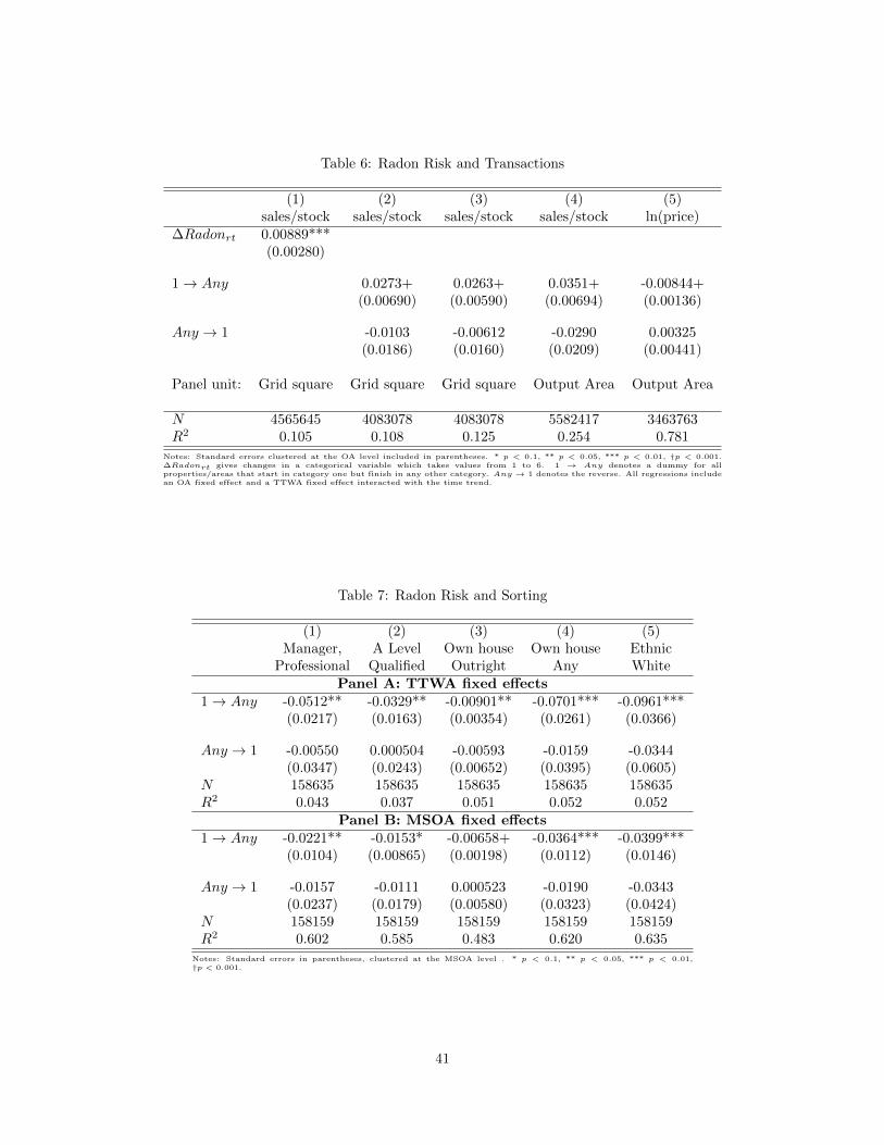
Table 6: Radon Risk and Transactions

(1) (2) (3) (4) (5)sales/stock sales/stock sales/stock sales/stock ln(price)

∆Radonrt 0.00889***(0.00280)

1→ Any 0.0273+ 0.0263+ 0.0351+ -0.00844+(0.00690) (0.00590) (0.00694) (0.00136)

Any → 1 -0.0103 -0.00612 -0.0290 0.00325(0.0186) (0.0160) (0.0209) (0.00441)

Panel unit: Grid square Grid square Grid square Output Area Output Area

N 4565645 4083078 4083078 5582417 3463763R2 0.105 0.108 0.125 0.254 0.781

Notes: Standard errors clustered at the OA level included in parentheses. * p < 0.1, ** p < 0.05, *** p < 0.01, †p < 0.001.∆Radonrt gives changes in a categorical variable which takes values from 1 to 6. 1 → Any denotes a dummy for allproperties/areas that start in category one but finish in any other category. Any → 1 denotes the reverse. All regressions includean OA fixed effect and a TTWA fixed effect interacted with the time trend.

Table 7: Radon Risk and Sorting

(1) (2) (3) (4) (5)Manager, A Level Own house Own house Ethnic

Professional Qualified Outright Any WhitePanel A: TTWA fixed effects

1→ Any -0.0512** -0.0329** -0.00901** -0.0701*** -0.0961***(0.0217) (0.0163) (0.00354) (0.0261) (0.0366)

Any → 1 -0.00550 0.000504 -0.00593 -0.0159 -0.0344(0.0347) (0.0243) (0.00652) (0.0395) (0.0605)

N 158635 158635 158635 158635 158635R2 0.043 0.037 0.051 0.052 0.052

Panel B: MSOA fixed effects1→ Any -0.0221** -0.0153* -0.00658+ -0.0364*** -0.0399***

(0.0104) (0.00865) (0.00198) (0.0112) (0.0146)

Any → 1 -0.0157 -0.0111 0.000523 -0.0190 -0.0343(0.0237) (0.0179) (0.00580) (0.0323) (0.0424)

N 158159 158159 158159 158159 158159R2 0.602 0.585 0.483 0.620 0.635

Notes: Standard errors in parentheses, clustered at the MSOA level . * p < 0.1, ** p < 0.05, *** p < 0.01,†p < 0.001.

41

Table 8: Placebo and Robustness Tests

(1) (2) (3) (4) (5) (6)Placebo Radon Tests House Fixed Effects

∆ln(price) ∆ln(price) ∆ln(price) ∆ln(price) ln(price) ln(price)

1→ Any 0.00187 -0.00204 -0.0157+ -0.0173*** -0.0138+ -0.0128**(0.00244) (0.0191) (0.00258) (0.00559) (0.00161) (0.00535)

Area Fixed Effects: TTWA OA TTWA OA TTWA OA

N 589234 130631 490484 127748 2433059 1755151R2 0.248 0.704 0.252 0.707 0.958 0.978

Notes: Standard errors in parentheses clustered at the 1km grid. * p < 0.1, ** p < 0.05, *** p < 0.01, †p < 0.001. The results in columns 1-4 arebased on pairs of transactions that occurred after 2010 (using the same map). The placebo change in radon applied to those pairs is based on thechange the house experienced when maps changed between 2003 and 2007. It is a falsification test. The dependent variable is price so that theresults are equivalent to table 4. 1 → Any denotes a dummy for all properties/areas that start in category one but finish in any other category.Any → 1 denotes the reverse. Columns 5 and 6 give results of a reclassification from no radon to any other category (again equivalent to table 4in areas where no more than 1% of houses have been tested for radon risk by PHE.

42

A Appendix

Table A1: Correlation between ambient air pollution (PM10) and radonrisk.

(1) (2) (3)PM10 2003 PM10 2008 Change in PM10

OA radon 2003 0.00233(0.00563)

OA radon 2008 0.00284(0.00286)

Change in OA radon 0.00502(0.00543)

N 153640 153578 153578R2 0.992 0.993 0.991

Notes: Standard errors in parentheses, clustered on MSOA and year * p < 0.1, ** p < 0.05, *** p < 0.01,†p < 0.001. All regressions inlcude an MSOA fixed effect. OA radon measures are maximum values in thearea. PM10 concentration is based on air pollution readings from the three closest DEFRA monitoringstations (weighted by inverse squared distance). Change in PM10 refers to the change in levels between2008 and 2003.

Table A2: Boundary discontinuity estimates of the impact of radonon house prices.

(1) (2) (3) (4)ln(price) ln(price) ln(price) ln(price)

Radon affected -0.00786 -0.00784 -0.00962** -0.0114**(0.00643) (0.00557) (0.00379) (0.00482)

TTWA FE Yes Yes Yes YesTime FE Yes Yes Yes YesDist. poly. Yes Yes Yes YesProp. char. Yes Yes YesOA char. Yes YesDistance limit 300m 300m 300m 500mN 99156 98706 98706 160927R2 0.447 0.664 0.770 0.763

Notes: Standard errors in parentheses, clustered on TTWA * p < 0.1, ** p < 0.05, *** p < 0.01.TTWA denote travel to work areas, Time FE refers to the quarter of the transaction, Dist. poly.denotes distance to the boundary and its polynomials (up to the third order). Prop. char. denotesproperty characteristics; property type, new/existing, urban/non-urban interacted with TTWAFE. OA char. denotes micro-neighbourhood characteristics as shares of population; in social classA, with A levels as the highest level of education, owning their houses, identifying as white, andowning their houses outright. Distance limit denotes the maximum distance to the boundary forproperties included in the BDD sample.

43

Table A3: The impact of radon on house prices –transactions with mortgages.

(1) (2)∆ln(price) ∆ln(price)

1→ 2 -0.0240*** -0.0164+(0.00676) (0.00278)

1→ 2 with Mortgage 0.0255 -0.00403(0.0178) (0.0108)

Time trend×area OA TTWAN 128016 493030R2 0.704 0.251

Notes: Standard errors in parentheses, clustered on 1km grid and yearpairs * p < 0.1, ** p < 0.05, *** p < 0.01, †p < 0.001. Column 1includes OA fixed effects interacted with time trends, the starting levelof radon and a dummy that equals one if the 25m grid is available in thearea/period, while column 2 replicates this using TTWA fixed effects.Both regressions include a dummy control for the property being newat the first sale. 1 → 2 with Mortgage is a dummy variable that equalsone if the transaction is funded by a Nationwide mortgage and receivesthe treatment. The OA sample includes a total of 597 properties with amortgage while the TTWA sample has 2,440.

Table A4: Estimation differences using the 25m or the 1km gridradon maps.

(1) (2) (3)∆ln(price) ∆ln(price) ∆ln(price)

1→ 2 25m grid -0.0261* -0.0213**(0.0126) (0.00969)

1→ 2 1km grid -0.0212** 0.00348 0.000390(0.00975) (0.0157) (0.0156)

Sample FULL 25m grid only 25m grid onlyObservations 127949 27847 27847R2 0.704 0.694 0.695

Notes: Standard errors in parentheses, clustered on 1km grid squares * p < 0.1, ** p < 0.05,*** p < 0.01, †p < 0.001. All regressions include an OA fixed effects interacted with timetrends. Column 1 compares the impact of radon depending on whether the best available infor-mation comes from the 25m grid or the 1km grid. Column 2 shows the impact of the 1km gridinformation in a sample where 25m grid data is available. Column 3 shows the impact of 25mgrid information and 1km grid information in locations where 25m grid information is available.

Table A5: Heterogeneity

(1) (2) (3) (4) (5)1→ Any -0.0193*** -0.0185** -0.0237** -0.0194** -0.0195*

(0.00636) (0.00705) (0.00936) (0.00754) (0.0103)

× Interaction 0.00179 -0.00411 0.0109 0.000296 0.000323(0.0286) (0.0248) (0.0145) (0.0147) (0.0121)

Interaction: Basement Rural Below p50 Above p50 Below p50Qualifications Deprivation Radon 2003

N 134734 134734 134734 134734 134734R2 0.704 0.704 0.704 0.704 0.704

Notes: Standard errors in parentheses, clustered on 1km grid * p < 0.1, ** p < 0.05, *** p < 0.01, †p < 0.001. All regressionsinclude Output Area fixed effects. Interaction terms for columns are: (1) address field suggests living accommodation is inbasement; (2) rural location; (3) residents in n’hood (OA) have below median qualifications (A levels or equivalent); (4) n’hood(LSOA) has above median level of deprivation; (5) labour-market area (TTWA) had below median radon in 2003.

44

Figure A1: Radon Risk Maps for Sheffield LAD: 1km2 and 25m2 grid maps.

Notes: The maps give the level of radon risk from 1 to 5 in the Sheffield LAD for the 1km squared grid map and for the more detailed 25m squaredmap.

45

Figure A2: Example of the radon-related demand and answer provided in CON29 form.

Source: UK Law Society - https://www.lawsociety.org.uk/en/topics/property/con29-forms.

46