The polytropic index of solar coronal plasma in sunspot fan loops andits temperature dependence

Krishna Prasad, S., Raes, J. O., Van Doorsselaere, T., Magyar, N., & Jess, D. B. (2018). The polytropic index ofsolar coronal plasma in sunspot fan loops and its temperature dependence. The Astrophysical Journal, 868, 1-9.[149]. https://doi.org/10.3847/1538-4357/aae9f5

Published in:The Astrophysical Journal

Document Version:Publisher's PDF, also known as Version of record

Queen's University Belfast - Research Portal:Link to publication record in Queen's University Belfast Research Portal

Publisher rights© 2018. The American Astronomical Society. All rights reserved.This work is made available online in accordance with the publisher’spolicies. Please refer to any applicable terms of use of the publisher.

General rightsCopyright for the publications made accessible via the Queen's University Belfast Research Portal is retained by the author(s) and / or othercopyright owners and it is a condition of accessing these publications that users recognise and abide by the legal requirements associatedwith these rights.

Take down policyThe Research Portal is Queen's institutional repository that provides access to Queen's research output. Every effort has been made toensure that content in the Research Portal does not infringe any person's rights, or applicable UK laws. If you discover content in theResearch Portal that you believe breaches copyright or violates any law, please contact openaccess@qub.ac.uk.

Download date:16. May. 2020

The Polytropic Index of Solar Coronal Plasma in Sunspot Fan Loops and ItsTemperature Dependence

S. Krishna Prasad1 , J. O. Raes2, T. Van Doorsselaere2 , N. Magyar2, and D. B. Jess1,31 Astrophysics Research Centre, School of Mathematics and Physics, Queen’s University Belfast, Belfast, BT7 1NN, UK; krishna.prasad@qub.ac.uk

2 Centre for mathematical Plasma Astrophysics, KU Leuven, Celestijnenlaan 200B, 3001 Leuven, Belgium3 Department of Physics and Astronomy, California State University Northridge, Northridge, CA 91330, USAReceived 2018 August 24; revised 2018 October 17; accepted 2018 October 18; published 2018 December 4

Abstract

Observations of slow magneto-acoustic waves have been demonstrated to possess a number of applications incoronal seismology. Determination of the polytropic index (γ) is one such important application. Analyzing theamplitudes of oscillations in temperature and density corresponding to a slow magneto-acoustic wave, thepolytropic index in the solar corona has been calculated and, on the basis of the obtained value, it has been inferredthat thermal conduction is highly suppressed in a very hot loop, in contrast to an earlier report of high thermalconduction in a relatively colder loop. In this study, using Solar Dynamics Observatory/AIA data, we analyzedslow magneto-acoustic waves propagating along sunspot fan loops from 30 different active regions and computedpolytropic indices for several loops at multiple spatial positions. The obtained γ values vary from 1.04±0.01 to1.58±0.12 and, most importantly, display a temperature dependence indicating higher γ at hotter temperatures.This behavior brings both the previous studies to agreement, and perhaps implies a gradual suppression of thermalconduction with increase in temperature of the loop. The observed phase shifts between temperature and densityoscillations, however, are substantially larger than that expected from the classical Spitzer thermal conduction, andappear to be influenced by a line-of-sight integration effect on the emission measure.

Key words: magnetohydrodynamics (MHD) – methods: observational – Sun: corona –

Sun: fundamental parameters

1. Introduction

Slow magneto-acoustic waves have been regularly observedin the solar corona since their initial discovery in polar plumes(Ofman et al. 1997, 1999; Deforest & Gurman 1998) andcoronal loops (Berghmans & Clette 1999; De Moortel et al.2000). Both propagating and standing versions of these waveshave been found, and their properties have been extensivelystudied using observations and theoretical modeling (seereview articles by De Moortel 2009 and Wang 2011). Standingslow waves are mainly observed in flare-related hot loopstructures (Wang et al. 2002, 2005; Kumar et al. 2015; Mandalet al. 2016; Nisticò et al. 2017, see Pant et al. 2017 for anexception) and are relatively rare, whereas propagating slowwaves have a photospheric source (Marsh & Walsh 2006; Jesset al. 2012; Krishna Prasad et al. 2015) and are more commonand ubiquitous in warm loops (De Moortel et al. 2002;McEwan & de Moortel 2006; Kiddie et al. 2012; KrishnaPrasad et al. 2012b, 2014). Modern high-resolution observa-tions have significantly improved our knowledge on slowwaves and have also revealed a wealth of seismologicalapplications.

Using stereoscopic observations of slow waves fromSTEREO/EUVI, Marsh et al. (2009) estimated their truepropagation speed and thereby deduced the temperature of theassociated loop. Wang et al. (2009), employing spectroscopicobservations of slow waves from EUV Imaging Spectrometer(EIS) on board Hinode (Culhane et al. 2007), obtained theinclination angle of a loop in addition to the correspondingplasma temperature. Van Doorsselaere et al. (2011) reportedthe measurement of polytropic index in the solar corona for thefirst time from the observations of slow waves using spectro-scopic data from EIS. Wang et al. (2015) made a similar

measurement for the plasma in a hot flare coronal loop utilizingthe observations of standing slow waves. Applying thedependence of the slow wave propagation speed on themagnetic field for high plasma-β loops, the coronal magneticfield has been estimated from both standing (Wang et al. 2007)and propagating waves (Jess et al. 2016). Utilizing theobservations of accelerating slow magneto-acoustic waves inmultiple channels, Krishna Prasad et al. (2017) obtainedthe spatial variation of temperature along a coronal loop inaddition to revealing its underlying multithermal structure(King et al. 2003).Our main focus in this study, however, is the determination

of a polytropic index. There have been several studies in thepast on the estimation of polytropic index using solar windproperties (e.g., Parker 1963; Roosen 1969; Kartalev et al.2006), but our emphasis here is on the particular application ofthe observations of slow magneto-acoustic waves. It has beenshown that thermal conduction introduces a phase lag betweentemperature and density perturbations of a slow magneto-acoustic wave (Owen et al. 2009). Also, from simple linearizedmagnetohydrodynamics (MHD) theory for slow waves, onecan show that the relative amplitudes of perturbations intemperature and density are directly related through thepolytropic index (Goossens 2003). Applying these, VanDoorsselaere et al. (2011) derived a polytropic index,γ=1.10±0.02, and inferred that thermal conduction is veryefficient in the solar corona. The authors obtained the requiredtemperature and density information from spectroscopic lineratios. Furthermore, through a comparison between temperatureand magnetic field fluctuations found from spectropolarimetricinversions of upper-chromospheric sunspot observations,Houston et al. (2018) also uncovered a similar polytropicindex, γ=1.12±0.01. Wang et al. (2015), on the other hand,

The Astrophysical Journal, 868:149 (9pp), 2018 December 1 https://doi.org/10.3847/1538-4357/aae9f5© 2018. The American Astronomical Society. All rights reserved.

1

employed a differential emission measure (DEM) analysis onbroadband imaging observations of a hot flare loop exhibitingstanding slow magneto-acoustic oscillations to obtain a γ valueof 1.64±0.08, which is close to the adiabatic index (5/3).This implies that thermal conduction is highly suppressed inthis loop, in contrast to the results of Van Doorsselaere et al.(2011) and Houston et al. (2018). Extending this work, Wanget al. (2018) performed 1D MHD simulations to compare withthe observations and extract further information on excitationand damping mechanisms of slow waves. In this study, wefollow the approach of Wang et al. (2015) and analyzepropagating slow magneto-acoustic waves in different activeregion fan loops using multiband imaging observations.The details of observations, obtained results, and conclusionsare described in the following sections.

2. Observations

Fan-like coronal loops rooted in sunspots are selected from 30different active regions observed between 2011 and 2016, for thepresent study. Imaging sequences of 1-hour-long durations takenin six coronal channels—namely the 94Å, 131Å, 171Å, 193Å,211Å, and 335Å channels of the Atmospheric ImagingAssembly (AIA; Lemen et al. 2012) on board the SolarDynamics Observatory (SDO; Pesnell et al. 2012)—are particu-larly utilized. AIA cutout data with subfields of about180″×180″ encompassing the individual fan-loop structureswere obtained and processed for all the six channels using arobust pipeline developed by Rob Rutten in IDL.4 Besidesapplying the necessary roll angle and plate scale corrections tothe downloaded level 1.0 data using aia_prep.pro (bringingthem to science-grade level 1.5), this pipeline aligns images frommultiple channels and corrects for any time-dependent shiftsusing a large subfield disk center data obtained at a lowercadence. Subpixel alignment accuracies of about 0 1 aretypically achieved even for the target subfields away from diskcenter. The spatial and temporal resolutions of the final data areabout 0 6 and 12 s, respectively. Figure 1 displays the vicinity ofthe selected fan-loop structures from all the 30 active regionsusing snapshots from the AIA 171Å channel. The start times ofthe individual data sets along with the corresponding NOAAnumbers are listed in the figure. The central coordinates, theoscillation period, and other important parameters obtained in thisstudy are listed in Table 1.

3. Analysis and Results

Fan-like loop structures from each of the selected activeregions were manually inspected for propagating oscillations,and a loop segment has been chosen where the oscillationsshow large amplitudes. These loop segments are shown as solidblue lines in Figure 1. In about five cases, we found anadditional loop segment displaying oscillations with reasonablygood amplitudes. These structures are marked with red solidlines in Figure 1. We constructed time-distance maps (e.g.,Berghmans & Clette 1999; De Moortel et al. 2000) for all thechosen loop segments following a method similar to thatdescribed in Krishna Prasad et al. (2012a). Although theselection of loop segments was mainly based on data from theAIA 171Å channel, similar time-distance maps were createdfor all six AIA coronal channels using cospatial segments. The

respective intensities from all the six channels were thensubjected to the regularized inversion code developed byHannah & Kontar (2012) to obtain the DEM at each spatial andtemporal position along the loop structure.A sample DEM profile is shown in Figure 2(c). The plus

symbol in red along the loop segment shown in Figure 2(a)marks the location from where the sample profile has beenextracted. As can be seen, the DEM profile is double peaked,with its first peak just under 1 MK (log10T=6.0) and itssecond peak near 2 MK (log10T=6.3) temperatures. The firstpeak is relatively stronger and broader, which represents thedominant emission coming from the loop, whereas the secondpeak appears to be likely due to the foreground/backgroundemission. Nearly all the loop structures analyzed in this studyexhibit a similar behavior. Figure 2(b) shows the temporallyaveraged DEM depicting its spatial variation along the loopstructure. Note that the horizontal axis in this figure shows thedistance along the loop, whereas the vertical axis displays thetemperature in logarithmic scale. Apparently, the double-peaked behavior is visible all along the loop and the dominantemission is coming from the low-temperature peak throughoutthe length, except for the bottom few arcseconds, where theforeground/background emission dominates. To properlyisolate the loop emission, we employed a best-fit double-Gaussian model for the DEM profiles. The solid line inFigure 2(c) shows the obtained fit to the data, whereas thedotted lines show individual Gaussians. The temperature atwhich the first Gaussian peaks is then considered as a measureof the loop temperature, whereas the area under this curveprovides the total emission measure. Following Sun et al.(2013) and Wang et al. (2015), we restrict the areameasurement to±2σ, where σ is the width of the Gaussiancurve. The emission measure (EM) and electron number

density (n) of the loop are related as n EM

d= , where d is

the depth of the loop along the line of sight. Considering asymmetric cross-section for the loop, the depth is thenestimated from the width of a Gaussian fitted to the cross-sectional intensity profile of the loop. A suitable location ismanually identified along each of the selected loop segmentswhere the cross-sectional profile could be better fitted with aGaussian, and the width estimated from that location isconsidered as the depth of the loop segment throughout itslength. As it follows, our main analysis is restricted to a fewarcseconds length along each loop structure, which makes thisapproximation reasonable. The estimated loop widths rangefrom 3–7 AIA pixels (1–3 Mm). The density and temperaturevalues thus obtained are used to build time-distance maps inthese quantities for each of the selected loop segments.Sample time-distance maps in intensity, temperature, and

density obtained from the loop segment marked in Figure 2(a)are shown in Figure 3. The time-distance map in intensityshown here is for the data from the AIA 171Å channel. Theslanted bright/dark ridges in each of these parameters highlightthe compressive oscillations propagating along the loop. Toenhance the visibility of these ridges, the time series at eachspatial position has been filtered in the Fourier domain,suppressing oscillation power outside a narrow band around thestrongest oscillation period. To achieve this, the Fourier powerof the respective time series were multiplied by a normalizedGaussian centered at the oscillation period with a width of1minute, before applying the inverse Fourier transform thatprovides the filtered time series (see, e.g., Jess et al. 2017). The4 http://www.staff.science.uu.nl/~rutte101/rridl/sdolib/

2

The Astrophysical Journal, 868:149 (9pp), 2018 December 1 Prasad et al.

oscillation period is predetermined through a simple Fourieranalysis of the AIA 171Å time series extracted from theaverage intensities over three adjacent pixel positions close to

the bottom of the loop foot point. The average time series hasbeen detrended to remove fluctuations of 6 minutes or longerbefore establishing the exact oscillation period.

Figure 1. AIA 171 Å images displaying fan-like loop structures from 30 different active regions observed between 2011 and 2016. The respective start times andNOAA numbers are printed on the figure. The solid lines in blue and red represent selected loop segments from individual regions. Blue and red segments correspondto “loop1,” and “loop2,” respectively, as listed in Table 1.

3

The Astrophysical Journal, 868:149 (9pp), 2018 December 1 Prasad et al.

It may be noted that the compressive oscillations decayrapidly as they propagate along the loop. Therefore, the time-distance maps presented in Figure 3 are shown only for a smallsection near the bottom of the loop where the amplitudes aresignificant. Nevertheless, as can be seen, the temperatureperturbations appear to decay faster than those of the density/intensity, a possible consequence of thermal conduction. Onemay also note that the amplitude of oscillations is not uniformthroughout the duration. At certain times (e.g., between 20 and35 minutes from the beginning of the time series in Figure 3),the oscillation amplitude is very much reduced in all threeparameters. Therefore, using the entire time series to determinephase shifts between temperature and density perturbations willproduce inaccurate results. Consequently, we restrict the phasedifference calculation to a particular range in time and spacewhere the amplitudes are large. This region is shown by theboxes in black dotted lines in Figure 3. A similar region hasbeen manually selected for all the loop structures by visuallyinspecting individual time-distance maps, particularly those oftemperature. The key restriction that we imposed while doingthis selection is that the region should contain at least threecycles of oscillations in both temperature and density. It may be

noted that, on the basis of this criterion, we could not findtemperature perturbations with sufficient signal in a couple ofcases, which, therefore, could not be utilized in furthercalculations (see Table 1).Figure 4(a) displays relative oscillations in temperature and

density within the chosen time range corresponding to the pixelposition marked by a white-dashed line in Figure 3. Verticalbars, here, denote the uncertainties in respective parameterspropagated from the errors on Gaussian fit to DEM curves. Itmay be noted that the temperature perturbations are consider-ably smaller than the corresponding density perturbations, asone would expect from a linearized MHD theory for slowwaves. Using a cross-correlation technique, we measure thetime lag (Δt) between the two parameters and then compute thecorresponding phase lag (Δf) from it following the relationΔf=(Δt/P)×360, where P is the oscillation period. Theobtained phase difference in this case is about +124°.5.Figure 4(b) shows a zoomed-in view of the oscillations (withinthe black dotted box in Figure 4(a)) with a separate scale fortemperature and density to clearly highlight the observed phasedifference between the quantities. The corresponding uncer-tainties are not shown here for clarity.

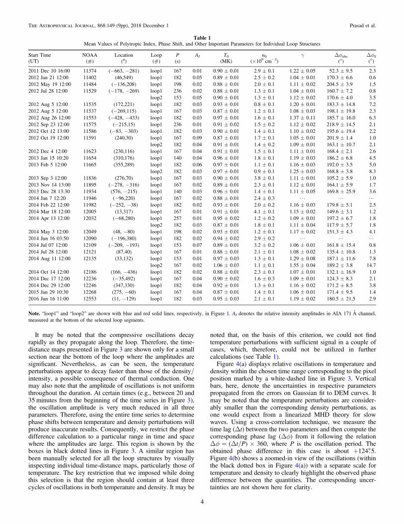
Table 1Mean Values of Polytropic Index, Phase Shift, and Other Important Parameters for Individual Loop Structures

Start Time NOAA Location Loop P AI T0 n0 γ Δfobs ΔfS(UT) (#) (″) (#) (s) (MK) (×109 cm−3) (°) (°)

2011 Dec 10 16:00 11374 (−663, −281) loop1 167 0.01 0.90±0.01 2.9±0.1 1.22±0.05 52.3±9.5 2.32012 Jan 21 12:00 11402 (46,549) loop1 182 0.05 0.89±0.01 2.5±0.2 1.04±0.01 170.3±6.6 0.62012 May 19 12:00 11484 (−136,208) loop1 198 0.02 0.88±0.01 2.0±0.1 1.11±0.02 204.5±3.9 1.52012 Jul 28 12:00 11529 (−178, −269) loop1 236 0.02 0.88±0.01 1.3±0.1 1.04±0.01 160.7±7.2 0.8

loop2 153 0.05 0.90±0.01 1.3±0.1 1.12±0.02 170.6±4.0 3.52012 Aug 5 12:00 11535 (172,221) loop1 182 0.03 0.93±0.01 0.8±0.1 1.20±0.01 183.3±14.8 7.22012 Aug 5 12:00 11537 (−269,115) loop1 167 0.03 0.87±0.01 1.2±0.1 1.08±0.03 198.1±19.8 2.32012 Aug 26 12:00 11553 (−428, −433) loop1 182 0.03 0.97±0.01 1.6±0.1 1.37±0.11 185.7±16.0 6.32012 Sep 23 12:00 11575 (−215,15) loop1 236 0.01 0.91±0.02 1.5±0.2 1.12±0.02 218.9±14.5 2.12012 Oct 12 13:00 11586 (−83, −303) loop1 182 0.03 0.90±0.01 1.4±0.1 1.10±0.02 195.6±19.4 2.22012 Oct 19 12:00 11591 (240,30) loop1 167 0.09 0.87±0.01 1.7±0.1 1.05±0.01 201.9±1.4 1.0

loop2 182 0.04 0.91±0.01 1.4±0.2 1.09±0.01 163.1±10.7 2.12012 Dec 4 12:00 11623 (230,116) loop1 167 0.04 0.91±0.01 1.5±0.1 1.11±0.01 168.4±2.1 2.62013 Jan 15 10:20 11654 (310,176) loop1 140 0.04 0.96±0.01 1.8±0.1 1.19±0.03 186.2±6.8 4.52013 Feb 5 12:00 11665 (355,289) loop1 182 0.06 0.97±0.01 1.1±0.1 1.16±0.03 192.0±3.5 5.0

loop2 182 0.03 0.97±0.01 0.9±0.1 1.25±0.03 168.8±3.8 8.32013 Sep 3 12:00 11836 (276,70) loop1 167 0.03 0.90±0.01 3.8±0.1 1.11±0.01 105.2±5.9 1.02013 Nov 14 13:00 11895 (−278, −316) loop1 167 0.02 0.89±0.01 2.3±0.1 1.12±0.01 164.1±5.9 1.72013 Dec 28 13:30 11934 (576, −215) loop1 140 0.03 0.96±0.01 1.4±0.1 1.11±0.05 169.8±25.9 3.62014 Jan 7 12:20 11946 (−96,220) loop1 167 0.02 0.88±0.01 2.4±0.3 L L L2014 Feb 22 12:00 11982 (−252, −38) loop1 182 0.02 0.93±0.01 2.0±0.2 1.16±0.03 179.8±5.1 2.52014 Mar 18 12:00 12005 (13,317) loop1 167 0.01 0.91±0.01 4.1±0.1 1.15±0.02 149.6±3.1 1.22014 Apr 13 12:00 12032 (−68,280) loop1 257 0.01 0.95±0.02 1.2±0.2 1.09±0.01 197.2±6.7 1.8

loop2 182 0.03 0.87±0.01 1.8±0.1 1.11±0.04 117.9±5.7 1.82014 May 3 12:00 12049 (48, −80) loop1 198 0.02 0.93±0.01 1.2±0.1 1.17±0.02 151.3±4.3 4.12014 Jun 16 03:50 12090 (−196,380) loop1 182 0.02 0.94±0.02 2.9±0.2 L L L2014 Jul 07 12:00 12109 (−209, −193) loop1 153 0.07 0.89±0.01 3.2±0.2 1.06±0.01 161.8±15.4 0.82014 Jul 28 12:00 12121 (87,40) loop1 167 0.01 0.88±0.01 2.1±0.1 1.08±0.02 135.4±10.8 1.32014 Aug 11 12:00 12135 (33,132) loop1 153 0.01 0.97±0.03 1.3±0.1 1.29±0.08 187.1±11.6 7.8

loop2 167 0.02 1.06±0.03 1.1±0.1 1.55±0.04 189.2±3.8 14.72014 Oct 14 12:00 12186 (166, −436) loop1 182 0.02 0.88±0.01 2.3±0.1 1.07±0.01 132.1±16.9 1.02014 Dec 17 12:00 12236 (−35,492) loop1 167 0.04 0.90±0.02 1.6±0.3 1.09±0.01 124.3±8.3 2.12014 Dec 29 12:00 12246 (347,330) loop1 182 0.04 0.92±0.01 1.3±0.1 1.16±0.02 171.2±8.5 3.82015 Jan 29 10:30 12268 (275, −60) loop1 167 0.04 0.87±0.01 1.4±0.1 1.06±0.01 171.4±9.5 1.42016 Jun 16 11:00 12553 (11, −129) loop1 182 0.03 0.95±0.03 2.1±0.1 1.19±0.02 180.5±21.5 2.9

Note. “loop1” and “loop2” are shown with blue and red solid lines, respectively, in Figure 1. AI denotes the relative intensity amplitudes in AIA 171 Å channel,measured at the bottom of the selected loop segments.

4

The Astrophysical Journal, 868:149 (9pp), 2018 December 1 Prasad et al.

Following the linearized MHD theory for slow magneto-acoustic waves, including thermal conduction as a dampingmechanism (e.g., De Moortel & Hood 2003; Owen et al. 2009;Krishna Prasad et al. 2014), it can be shown that

T ı

ı n

cos sin cos

sin 1 , 1

dc k dc krel

rel

s s2 2 2 2

f f f

f g

D + D - D

+ D = -

gw

gw(

) ( ) ( )

where γ is the polytropic index, Δf is the phase shift betweendensity and temperature (introduced by thermal conduction),c ps 0 0g r= is the sound speed, d

k T

c p

1

s

0

20

=g

g

- ( )is the thermal

conduction parameter, ω is the angular frequency, k is thewavenumber, Trel=T T0¢ is the relative amplitude of temp-erature, and nrel=n n0¢ is the relative amplitude of density.n0, T0, ρ0, and p0 represent the equilibrium values of electronnumber density, temperature, mass density, and pressure,respectively. n′ and T′ denote the corresponding amplitudesof the perturbed values in electron number density andtemperature. k k T0 0

5 2= gives the parallel thermal conduction,where k0 is the thermal conduction coefficient. Equating theimaginary and real parts on both sides of Equation (1) gives

sin cos 0, 2dc ks2 2

f fD - D =gw

( )

T ncos sin 1 . 3dc krel rel

s2 2

f f gD + D = -gw( ) ( ) ( )

Using the definition of d, and p n k T20 0 B 0= , where kB is theBoltzmann’s constant, Equation (2) can be rewritten as

k

k c Pntan

14

sB2

0

fp g

D =- ( )

( )

(e.g., Van Doorsselaere et al. 2011; Wang et al. 2015). Here, Pis the time period of the oscillation. In addition, using

Equations (2) & (3), one may deduce

T n 1 cos . 5rel rel g f= - D( ) ( )

Equations (4) and (5) can be used to understand the observedamplitudes of temperature and density, and the phase shiftsbetween them. In the case of fully isothermal plasma, thepolytropic index, γ, is equal to 1; hence, as may be inferredfrom Equation (5), there would not be any perturbations intemperature. On the other hand, if the conditions are perfectlyadiabatic (i.e., γ=5/3) with negligible thermal conduction,Equation (4) gives Δf≈0, which implies from Equation (5)that the relative amplitude of temperature perturbations is about66% (2/3) of that of density perturbations, with no phase shiftbetween the quantities. For intermediate cases, the knowledgeof the polytropic index and thermal conduction coefficient isnecessary to accurately determine the values. Alternatively, onecan use the observed phase shifts and amplitude values toobtain the polytropic index and the thermal conductioncoefficient.As one might note from Equations (4) and (5), a valid

common solution exists only if the phase shift betweentemperature and density is between 0°and 90°. However, ascan be seen from Figure 4(b), the observed phase shift is about+124°.5, albeit for a single spatial position along the loopstructure shown in Figure 2(a). In fact, even other spatialpositions and nearly all the loop structures investigated in thisstudy show similar values well outside the expected range. Thisimplies that there is an additional source of phase shift inobservations and, consequently, that the observed valuescannot be directly used to obtain the thermodynamicparameters. However, considering the phase shift to be constantover the duration of the time series,5 one can eliminate the

Figure 2. Typical characteristics of obtained DEMs. (a) AIA 171 Å image showing the vicinity of a sunspot fan-loop structure from AR12236 as observed on 2014December 17, 12:00 UT. The solid blue lines represent the selected loop segment. (b) Time-averaged DEM plot for the loop segment shown in (a), displaying thespatial variation. The double-peaked nature of the DEM is visible throughout the length of the loop with dominant emission from the colder peak. (c) Sample DEMprofile from the pixel location marked by a red plus symbol in (a). The solid line represents a double-Gaussian fit to the data in red diamonds. The dotted lines markthe two individual Gaussians corresponding to the emission from the loop and the foreground/background emission.

5 This is a valid assumption because the physical conditions on which thephase shift is dependent (see Equation (4)) do not change appreciably over thetimescales involved.

5

The Astrophysical Journal, 868:149 (9pp), 2018 December 1 Prasad et al.

dependence on it from Equation (5) by merely shifting thetemperature (or density) time series to match the phasewith that of density (or temperature). This step reducesEquation (5) to

T n 1 , 6srel rel g= -( ) ( )

where Trels denotes the relative amplitudes of temperature shifted

to be in phase with density. Equation (6) can then be readily usedto obtain the polytropic index. In Figure 4(c), we plotT s

rel obtainedby shifting the temperature perturbations shown in Figure 4(a) by−124°.5 against the corresponding unshifted nrel. The error barshere denote the respective uncertainties in temperature. A linearrelationship between the parameters is evident from the data. Theoverplotted red solid line denotes the best linear fit obtained.Applying Equation (6), we calculate the polytropic index,γ=1.10±0.01, from the slope of the fitted line. The expecteddependence for adiabatic conditions (γ=5/3) is shown by adotted line in this figure, which is largely deviated from theactual data.

It is important to note here that Equation (6) is generallyapplicable for slow magneto-acoustic waves whether or not thereis thermal conduction. Of course, in cases of no thermalconduction, the temperature perturbations need not be shiftedbecause they are expected to be already in phase with density.However, it does not mean that, by removing the phase shiftdependence from Equation (5), we have completely eliminatedthe effects of thermal conduction. It is inherently assumed thatthe polytropic index, γ, is modified by the presence of thermalconduction, which should be reflected in the temperature anddensity amplitudes of a slow wave. Although this is true, in thecase of coronal plasma, the polytropic index is governed not justby the thermal conduction but also by several other importantprocesses, such as heating, radiative losses, turbulence, plasma

flows, and other nonthermal processes. Therefore, a γ valuelower than 5/3, as deduced from the observed amplitudes, neednot necessarily imply enhanced thermal conduction.Keeping these limitations in mind, we computed the

polytropic index at individual spatial positions across allthe selected loop structures following the same procedure. Theobtained values are plotted against the corresponding time-averaged temperature (logarithmic values) in Figure 5, usingdiamond symbols in black. For comparison, we also show theresults from Van Doorsselaere et al. (2011) and Wang et al.(2015) using a red triangle and a green square, respectively.The vertical bars in this figure represent the respectiveuncertainties. All our data, across 164 spatial positionsidentified from about 33 loop structures, are displayed in thisfigure. To clearly highlight the observed dependence from ourdata, a zoomed-in view is presented in the inset panel.Although our temperature range is limited because of ourselection of only fan-like warm loop structures, it appears thatthe polytropic index is increasing with the temperature.In Table 1, we list the mean values of temperature, T0, density,

n0, the polytropic index, γ, and the observed phase shift betweenthe temperature and density perturbations (Δfobs) for all the loopstructures studied. The uncertainties listed with these values areobtained from the respective standard deviations across eachloop. The small uncertainties suggest that the values themselvesdo not vary much within a loop structure. The limited spatialranges considered along each loop could also be partiallyresponsible for this. It may be noted that the temperature anddensity values obtained here are of the same order of those foundfrom spectroscopic observations of fan loops (Ghosh et al.2017). The relative intensity amplitudes and the oscillationperiods computed for individual loops are also listed. Theamplitudes are measured from the AIA 171Å channel, nearthe bottom of the selected loop structures where they are usually

Figure 3. Time-distance maps in AIA 171 Å intensity, temperature, and density, corresponding to the loop segment shown in Figure 2(a). Each of the maps wasFourier filtered, allowing power within a narrow band around the oscillation period to enhance the visibility of the ridges. The boxes in black dotted lines marked ontemperature and density maps bound the selected spatial and temporal ranges for phase lag analysis. The white-dashed line in these maps shows the spatial locationfrom which the temperature and density lightcurves plotted in Figure 4(a) are extracted.

6

The Astrophysical Journal, 868:149 (9pp), 2018 December 1 Prasad et al.

the highest. The values range from 0.01 to 0.09, suggesting thelinear nature of the observed waves. A majority of the oscillationperiods are near 180 s, which is not surprising considering thatthe selected loop structures are rooted mainly in sunspots. Inaddition, in the last column, we list the expected phase shifts(ΔfS) obtained using Equation (4), for the classical Spitzerthermal conductivity (k0=7.8×10−7; Spitzer 1962). Thepolytropic index, temperature, density, and the oscillation periodused in this calculation are from the observed values. While thevalues ΔfS range between 0°.5 and 15°, the observed phaseshifts, Δfobs, vary between 52°and 219°. Evidently, theobserved phase shifts are significantly larger than the corresp-onding values for the classical thermal conductivity. In a coupleof loops, the temperature perturbations do not possess sufficientamplitudes to estimate γ, Δfobs, and ΔfS, which, therefore, areleft blank.

4. Discussion and Conclusions

It has been demonstrated that the amplitudes of temperatureand density perturbations due to a slow magneto-acousticwave, and the phase shift introduced between them by thermalconduction, can be utilized to understand the thermodynamicproperties of solar coronal plasma. Using spectroscopic datafrom Hinode/EIS, Van Doorsselaere et al. (2011) have

Figure 4. Determination of phase shift and polytropic index. (a) Perturbations in temperature and density from the spatial location marked by the white-dashed lines inFigure 3. The vertical bars show the respective uncertainties propagated from the errors on Gaussian fit to DEM curves. (b) A zoomed-in view of the oscillationswithin the black dotted box in (a), with an independent scale for density and temperature, mainly to highlight the observed phase shift between the quantities. Thecorresponding uncertainties are not shown here for clarity. (c) A scatter plot of relative temperature (with respective uncertainties as error bars) plotted againstthe relative density from (a) after shifting the temperature values to remove the existing phase shift. The red solid line represents the best linear fit to the data. Thepolytropic index obtained from the slope of the line is listed in the plot. The dotted line shows the expected dependence for adiabatic conditions (γ=5/3).

Figure 5. Dependence of polytropic index on mean temperature. Here, γ valuesobtained from individual spatial positions across all the selected loop segmentsare plotted against the corresponding time-averaged temperature. The diamondsymbols in black represent the data from this study, whereas the red triangleand the green square represent the data from Van Doorsselaere et al. (2011),and Wang et al. (2015), respectively. The vertical bars show the respectiveuncertainties on the values. A zoomed-in view of our data is provided in theinset panel to clearly highlight the observed dependence.

7

The Astrophysical Journal, 868:149 (9pp), 2018 December 1 Prasad et al.

obtained the polytropic index, γ=1.10±0.02, for a warmcoronal loop and have inferred that thermal conduction is veryefficient in the solar corona. More recently, Wang et al. (2015)have performed a similar analysis on a hot flare loop andobtained γ=1.64±0.08, suggesting, in contrast, a suppres-sion in thermal conduction. Although the relevant spectro-scopic data were not available, Wang et al. (2015) haveextracted the required temperature and density informationfrom broadband SDO/AIA images in multiple coronalchannels through DEM analysis. Following the latter approach,we studied propagating slow magneto-acoustic waves in about30 different active regions, particularly those in fan-like loopstructures. Employing a regularized inversion method (Hannah& Kontar 2012) on the observed intensities in six AIA coronalchannels, corresponding DEMs have been obtained. The DEMprofiles mostly displayed a double-peaked structure, with onebroader dominant peak around 1 MK representing the loopemission and another narrow peak near 2 MK representing theforeground/background emission. We carefully isolated theloop emission using the best-fit double-Gaussian profiles andcomputed respective electron temperatures and densities (viaemission measure) to construct time-distance maps in thoseparameters along selected loop segments. For each loopstructure, a limited range in temporal and spatial domains isidentified near the bottom of the loop, where the amplitudes ofoscillation are large enough to accurately calculate the phaseshift between temperature and density. Within the selectedrange, the phase shift between the parameters is computedusing a cross-correlation method. The obtained values aresubstantially larger than that expected from the classical Spitzerthermal conductivity. Although this might mean that thethermal conduction is higher than the classical values, one mustnote that the observed values are even larger than that could bereconciled with the wave theory, which therefore suggests thatthe apparent phase shifts are not merely due to thermalconduction.

It is also worth noting that most of the observed phase shiftvalues are clustered around 180°(see Table 1). Jess et al. (2012)studied a sunspot fan-loop structure using an independent DEMmethod and found that the obtained peak temperature andemission measure are 180° out of phase. The authors explainedthis behavior as being due to the anticorrelated changes inemission volume along the line of sight. Although, from ourdata, we do not find a definitive dependence of phase shifts onthe location of the loop structure (perhaps because of thenonuniform distribution of our data with more samples towardthe solar disk center), it is possible that a similar effect isresponsible for the large phase shifts observed here. Forinstance, the loop structure that is furthest from the disk center(i.e., from AR11374) in our sample shows the smallest phaseshifts (≈52°). Besides, the temperature and density valuesobtained from our DEM analysis are representative of meanvalues over the cross-section of a loop, which implies themultithermal nature of the active region loops, as evidencedfrom the differential propagation of slow waves when observedin multiple temperature channels (Kiddie et al. 2012; Uritskyet al. 2013; Krishna Prasad et al. 2017), is not considered. Thisapproximation may also influence the observed phase shifts. Itmay also be worthwhile exploring whether the misbalance in thelocal thermal equilibrium caused by the slow waves (Nakariakovet al. 2017) can, in turn, affect the observed phase shifts.Additional effects, such as nonlinearity (Nakariakov et al. 2000;

Ofman & Wang 2002) and partial wave reflection, can affect thephase shifts but do not seem to be applicable to our data. In anycase, even in the absence of the aforementioned effects, the exactphase shift depends on several factors (see Equation (4)) and,hence, should not be assumed to correlate precisely with thermalconduction.By manually shifting the temperature time series to remove

the existing phase shift, we compare the oscillation amplitudesin temperature against that in density and compute thepolytropic index. These values occur in the range between1.04±0.01 and 1.58±0.12. It also appears that there is atemperature dependence, with hotter loops having a higherpolytropic index. Qualitatively, this behavior brings thecontrasting findings of Van Doorsselaere et al. (2011) andWang et al. (2015) to a good agreement. One may note,however, that the observed dependence of polytropic index ontemperature (see Figure 5) is steeper than what would berequired to have a better match with the previous results. Thiswarrants the requirement of additional examples distributedacross a wider temperature range to find the exact dependence.Moreover, the phase shift between the temperature and densityperturbations observed in the earlier studies is relatively small(<90°), unlike that in our case. Van Doorsselaere et al. (2011)obtained the temperature and density information directly fromthe spectroscopic line ratios, so their results are less prone tothe line-of-sight effect, which we believe is the cause for thelarge phase shifts in our data. However, it is intriguing whyWang et al. (2015) do not see any such effect. It is possible thatthe extremely hot plasma in their loop somehow helps inmitigating the line-of-sight changes, but this requires furtherstudies to confirm and improve our understanding of this effect.Finally, although it is possible that the increase in polytropic

index with temperature might imply a gradual suppression ofthermal conduction in agreement with the inferences fromprevious studies, it is much harder to explain. Wang et al.(2015) offered some explanations based on nonlocal conduc-tion, plasma waves, and turbulence that are more applicable tohot flare loops, but because this behavior appears to be moreprevalent even in the warm loops, one needs to find a generaltheory. Besides, the influence of other thermodynamicprocesses (e.g., heating and radiative losses), in addition tothe observational effects (e.g., multithermal structure of loops)on the polytropic index, should be investigated. We believe thatfuture studies, ideally a combination of observations, numericalsimulations, and forward modeling, might reveal importantinformation to address this problem.

The authors thank the anonymous referee for usefulcomments. S.K.P. is grateful to the UK Science andTechnology Facilities Council (STFC) for funding supportthat allowed this project to be undertaken. T.V.D. wassupported by grant No. GOA-2015-014 (KU Leuven) and theEuropean Research Council (ERC) under the EuropeanUnion’s Horizon 2020 Research and Innovation Programme(grant agreement No. 724326). D.B.J. would like to thankSTFC for an Ernest Rutherford Fellowship, in addition toInvest NI and Randox Laboratories Ltd. for the award of aResearch & Development Grant (059RDEN-1). AIA data usedhere are courtesy of NASA/SDO and the AIA science team.We acknowledge the use of pipeline developed by Rob Ruttento extract, process, and coalign AIA cutout data.

8

The Astrophysical Journal, 868:149 (9pp), 2018 December 1 Prasad et al.

ORCID iDs

S. Krishna Prasad https://orcid.org/0000-0002-0735-4501T. Van Doorsselaere https://orcid.org/0000-0001-9628-4113D. B. Jess https://orcid.org/0000-0002-9155-8039

References

Berghmans, D., & Clette, F. 1999, SoPh, 186, 207Culhane, J. L., Harra, L. K., James, A. M., et al. 2007, SoPh, 243, 19De Moortel, I. 2009, SSRv, 149, 65De Moortel, I., & Hood, A. W. 2003, A&A, 408, 755De Moortel, I., Ireland, J., & Walsh, R. W. 2000, A&A, 355, L23De Moortel, I., Ireland, J., Walsh, R. W., & Hood, A. W. 2002, SoPh, 209, 61Deforest, C. E., & Gurman, J. B. 1998, ApJL, 501, L217Ghosh, A., Tripathi, D., Gupta, G. R., et al. 2017, ApJ, 835, 244Goossens, M. 2003, An Introduction to Plasma Astrophysics and

Magnetohydrodynamics, Vol. 294 (Dordrecht: Kluwer)Hannah, I. G., & Kontar, E. P. 2012, A&A, 539, A146Houston, S. J., Jess, D. B., Asensio Ramos, A., et al. 2018, ApJ, 860, 28Jess, D. B., De Moortel, I., Mathioudakis, M., et al. 2012, ApJ, 757, 160Jess, D. B., Reznikova, V. E., Ryans, R. S. I., et al. 2016, NatPh, 12, 179Jess, D. B., Van Doorsselaere, T., Verth, G., et al. 2017, ApJ, 842, 59Kartalev, M., Dryer, M., Grigorov, K., & Stoimenova, E. 2006, JGRA, 111,

A10107Kiddie, G., De Moortel, I., Del Zanna, G., McIntosh, S. W., & Whittaker, I.

2012, SoPh, 279, 427King, D. B., Nakariakov, V. M., Deluca, E. E., Golub, L., & McClements, K. G.

2003, A&A, 404, L1Krishna Prasad, S., Banerjee, D., & Singh, J. 2012a, SoPh, 281, 67Krishna Prasad, S., Banerjee, D., & Van Doorsselaere, T. 2014, ApJ, 789, 118Krishna Prasad, S., Banerjee, D., Van Doorsselaere, T., & Singh, J. 2012b,

A&A, 546, A50Krishna Prasad, S., Jess, D. B., & Khomenko, E. 2015, ApJL, 812, L15Krishna Prasad, S., Jess, D. B., Klimchuk, J. A., & Banerjee, D. 2017, ApJ,

834, 103

Kumar, P., Nakariakov, V. M., & Cho, K.-S. 2015, ApJ, 804, 4Lemen, J. R., Title, A. M., Akin, D. J., et al. 2012, SoPh, 275, 17Mandal, S., Yuan, D., Fang, X., et al. 2016, ApJ, 828, 72Marsh, M. S., & Walsh, R. W. 2006, ApJ, 643, 540Marsh, M. S., Walsh, R. W., & Plunkett, S. 2009, ApJ, 697, 1674McEwan, M. P., & de Moortel, I. 2006, A&A, 448, 763Nakariakov, V. M., Afanasyev, A. N., Kumar, S., & Moon, Y.-J. 2017, ApJ,

849, 62Nakariakov, V. M., Verwichte, E., Berghmans, D., & Robbrecht, E. 2000,

A&A, 362, 1151Nisticò, G., Polito, V., Nakariakov, V. M., & Del Zanna, G. 2017, A&A,

600, A37Ofman, L., Nakariakov, V. M., & Deforest, C. E. 1999, ApJ, 514, 441Ofman, L., Romoli, M., Poletto, G., Noci, G., & Kohl, J. L. 1997, ApJL,

491, L111Ofman, L., & Wang, T. 2002, ApJL, 580, L85Owen, N. R., De Moortel, I., & Hood, A. W. 2009, A&A, 494, 339Pant, V., Tiwari, A., Yuan, D., & Banerjee, D. 2017, ApJL, 847, L5Parker, E. N. 1963, Interplanetary Dynamical Processes (New York: Interscience)Pesnell, W. D., Thompson, B. J., & Chamberlin, P. C. 2012, SoPh, 275, 3Roosen, J. 1969, SoPh, 7, 448Spitzer, L. 1962, Physics of Fully Ionized Gases (New York: Interscience)Sun, X., Hoeksema, J. T., Liu, Y., et al. 2013, ApJ, 778, 139Uritsky, V. M., Davila, J. M., Viall, N. M., & Ofman, L. 2013, ApJ, 778, 26Van Doorsselaere, T., Wardle, N., Del Zanna, G., et al. 2011, ApJL, 727,

L32Wang, T. 2011, SSRv, 158, 397Wang, T., Innes, D. E., & Qiu, J. 2007, ApJ, 656, 598Wang, T., Ofman, L., Sun, X., Provornikova, E., & Davila, J. M. 2015, ApJL,

811, L13Wang, T., Ofman, L., Sun, X., Solanki, S. K., & Davila, J. M. 2018, ApJ,

860, 107Wang, T., Solanki, S. K., Curdt, W., Innes, D. E., & Dammasch, I. E. 2002,

ApJL, 574, L101Wang, T. J., Ofman, L., Davila, J. M., & Mariska, J. T. 2009, A&A, 503, L25Wang, T. J., Solanki, S. K., Innes, D. E., & Curdt, W. 2005, A&A, 435,

753

9

The Astrophysical Journal, 868:149 (9pp), 2018 December 1 Prasad et al.