Reassessing Polytropic Compressor Calculations of ASME PTC 10

Energy Management Research Journal

Vol. 3, No. 1; 2020

Published by CanSRG

http://cansrg.com/journals/emrj/

* Corresponding author

Submitted: March 24, 2020 Accepted: May 28, 2020

Reassessing Polytropic Compressor Calculations of ASME PTC 10

R. A. Wilsak1 and R. A. Tatara2,* 1Racine, WI 53402, USA

2Department of Engineering Technology, Northern Illinois University, DeKalb, IL 60115, USA

Abstract

Centrifugal compressor calculations inherent to process simulators are based on

ASME PTC 10, which in turn is derived from the work of J. M. Schultz in the

1960s. Although the analysis from Schultz began with the reversible path

following a polytrope, this was negated once the polytropic exponent was

allowed to vary. Moreover, the path was altered on an inconsistent basis through

the use of a correction factor and piecewise integration of the reversible path with

various polytropic exponents. The result is an erroneous procedure embodied in

ASME PTC 10. Here, a new polytropic analysis with a precisely defined

reversible path is presented. The final equations are thermodynamically rigorous

subject to assumptions that the compressor is at steady state, the gas flowing

through the compressor is single phase and no chemical reactions take place.

Keywords: ASME PTC 10; Centrifugal Compressors; Polytropic Compression;

Process Simulators.

1. Introduction

Centrifugal compressors are routinely used in refrigeration loops and other processes whenever

the pressure of a gas needs to be increased. A common industrial example is an ethene/propene

cascaded refrigeration system wherein liquid ethene at temperatures ranging from -70 to -100°C

(-94 to -148°F) is supplied via an ethene refrigeration loop, but the system also requires a

propene refrigeration loop as a heat sink. Two centrifugal compressors are employed; one to

compress the ethene and another to compress the propene with the propene unit about four times

larger. A moderately sized system can require 15 MW (~20,000 hp) to power both compressors,

but much larger processes are being built in Asia, often three times the size. Many compressors

are driven by electrical motors, with the cost of electricity varying greatly depending on location.

The U.S. Energy Information Administration (EIA) compiles, analyzes and reports energy usage

and cost throughout the United States. As recently reported [1], the average cost of electricity for

industrial users ranged from a low of 5.20 cents per kW-hr (3.88 cents per hp-hr) in Louisiana to

a high of 25.21 cents per kW-hr (18.81 cents per hp-hr) in Hawaii during August of 2019. The

overall U.S. average was 7.44 cents per kW-hr (5.55 cents per hp-hr). Many oil refineries,

petrochemical plants and natural gas facilities are located in Texas where the August 2019

average cost was 7.51 cents per kW-hr (5.60 cents per hp-hr). Therefore, a moderately sized

ethene/propene refrigeration system located in Texas would consume about 1.2 x 108 kW-hr (1.6

x 108 hp-hr) of electricity annually, assuming a relatively low 90% operating factor, yielding

electrical costs of $9 million per year. Moreover, the EIA reports that only 21% of the U.S.

electrical generating capacity uses renewable energy sources with 68% still powered with fossil

fuels. Hence, suboptimal performance of centrifugal compressors will significantly increase both

operating cost for the end user and the release of greenhouse gases from electrical generating

companies.

Wilsak and Tatara Energy Management Research Journal Vol. 3, No. 1; 2020

14

Not all centrifugal compressors are powered by electrical motors. For example, cracked gas

compressors in olefins plants are typically driven by steam turbines where the high-pressure

steam that is used to power the turbines is produced from transfer line heat exchangers located

downstream of the pyrolysis furnaces. The heat exchangers cool the pyrolysis gas quickly in

order to improve the selectivity of the products. The cracked gas compressors are among the

largest centrifugal compressors, often reaching 40 MW (~54,000 hp). Improvements in

compressor operation will lower the steam requirement, which allows some of the high pressure

steam to be diverted to other uses within the plant, such as replacing a furnace that burns fuel

with a heat exchanger utilizing the steam. The benefits will again be economic due to less fuel

consumption and also environmental with the release of fewer greenhouse gases.

An industrial plant strives to optimize performance of its many unit operations, such as reactors,

heat exchangers, distillations columns and compressors. Modern computer programs can easily

solve problems involving hundreds or even thousands of unit operations. But in order to operate

the plant in a cost-effective manner, the simulation must contain well-written subroutines for

each type of unit operation; errors in the subroutines will skew the calculations resulting in a

suboptimal solution. For example, Li and Li [2] used commercial software from Aspen Plus

(Aspen Technology, Inc., Burlington, Massachusetts, USA) in their optimization of the cracked

gas compressor of an olefins plant. Since centrifugal compressors are common components of

industrial plants and since their impacts on cost and the environment are significant, it is

important that the underlying computer models for compressors be as accurate as possible. Users

of computer simulations rarely question the appropriateness of each subroutine that is called in a

plant optimizer. Thus, unfortunately, errors can be perpetuated as erroneous coding is passed

from one user to another with each assuming the coding had been previously verified.

For the calculation of centrifugal compressor performance, many simulators utilize a procedure

based on the standards established by the American Society of Mechanical Engineers known as

ASME PTC (performance test code) 10 [3]. This code is primarily concerned with the methods

used by vendors to test compressors, and much of it explains how to rate a new compressor. The

emphasis is to maintain dynamic similarity with the desired conditions, particularly in those

cases where the vendor is unable to test the compressor with the same gas or at the same

conditions as specified by the user. Only a portion of the code discusses how the compressor

calculations should be executed. Unfortunately, there are a number of typographical errors in the

equations given in Tables 5.1 and 5.2 which summarize the performance equations. Most of the

errors involve the misplacement of equation labels, brackets or equal signs. (For example, see

Equations (5.1T-3) and (5.1T-6) through (5.1T-8) in Table 5.1 and Equations (5.2T-3) and (5.2T-

6) through (5.2T-9) in Table 5.2.) The corresponding equations presented within the text, such as

Equations (5.3.2) and (5.3.3), are correct.

A significant issue is a thermodynamically incorrect procedure in ASME PTC 10 for evaluating

polytropic compressor performance. There are a number of publications in the literature that

discuss the limitations of the ASME PTC 10 procedure. For example, the recent article of

Sandberg and Colby [4] points out that the root causes for errors creeping into the analysis are

not fully understood. ASME PTC 10 is essentially based on the procedures proposed by Schultz

[5] to the Power Test Codes Committee of the American Society of Mechanical Engineers in

1960. In reviewing the work of Schultz, one is struck by how difficult it was in the 1950s to

calculate the physical properties of real gases, which is a problem largely eliminated through the

use of computer programs. The procedure was a practical approach wherein the process


15

equations for the compressor analysis were manipulated to provide a framework suitable for

using generalized charts for the physical properties of real gases. The charts were based on the

law of corresponding states and, while these generalized charts are now a footnote in engineering

history, their use by Schultz influenced the way these compressor calculations have been

performed ever since.

Unfortunately, the work of Schultz contains a fundamental flaw early in his development of the

polytropic compressor analysis, and this flaw has gone unrecognized ever since. Evans and

Huble [6] discuss various numerical integration methods to evaluate a key term in one of the

equations presented by Schultz. Furthermore, they provide summaries of eleven previous articles

addressing various ways to accurately perform polytropic compressor calculations. None

considers the possibility that Schultz’s analysis is in fact in error. In a series of papers, Taher [7-

9] discusses the importance of how to calculate the physical properties of real gases. In this

regard, Taher improves upon Schultz’s work concerning physical properties but does not

question Schultz’s given compressor equations. The recent work of Park et al. [10] follows the

ASME PTC 10 procedures in determining the performance of a centrifugal compressor using

alternative refrigerants that have low global warming impact. Therefore, the mistake in the early

work of Schultz continues to be perpetrated.

A new methodology for polytropic compressor calculations is presented herein. A key feature of

this methodology is that the formulation of the process equations is thermodynamically correct,

and unlike the method of Schultz and that of ASME PTC 10, no improper approximations were

invoked. Also, the simplifications used in developing our final equations are clearly delineated.

As the new approach is revealed, four items will be pointed out at the appropriate times that

should illuminate the meaning and highlight the restrictions involved with polytropic compressor

calculations: i) a precise description of the underlying reversible process that represents the

benchmark against which a real compressor is compared; ii) the reason that only homogeneous

mixtures are considered; iii) the restriction that chemical reactions should not occur in the

compressor; and iv) the proper way to handle often neglected energy terms such as kinetic

energy, potential energy and heat transfer. Finally, this work will discuss the difficulties that

arise when the methodology is extended from a single-section, or single-stage, compressor that

contains only a single inlet and a single outlet to a multi-section compressor that has more than

one inlet or outlet streams.

2. Thermodynamic Analysis

There are three thermodynamic equations that are used in the analysis of compressor

performance. These are the First Law of Thermodynamics (energy balance), the Second Law of

Thermodynamics (entropy balance) and the internal energy form of the fundamental property

relationship (U as a function of S, V and ni). Only two of these three equations are independent.

The analysis will begin with the application of these three equations to a single-section

compressor as illustrated in Figure 1. Following ASME PTC 10 convention, a single-section

compressor has no intermediate material streams entering or exiting the compressor, i.e., there

are no side-streams. Later in the discussion, we will expand this to a multi-section compressor. A

single-section compressor can, and often does, contain more than one impeller. Up to ten

impellers are common for a single section.


16

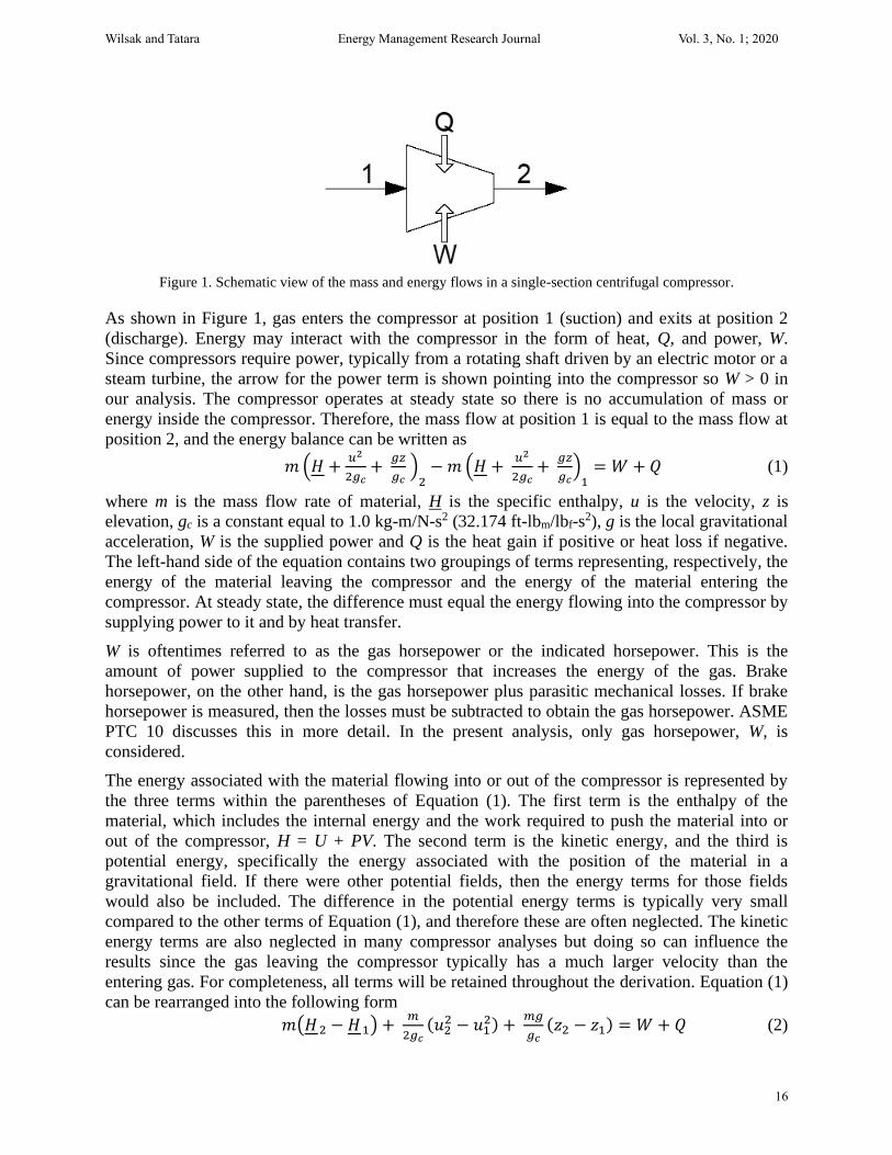
Figure 1. Schematic view of the mass and energy flows in a single-section centrifugal compressor.

As shown in Figure 1, gas enters the compressor at position 1 (suction) and exits at position 2

(discharge). Energy may interact with the compressor in the form of heat, Q, and power, W.

Since compressors require power, typically from a rotating shaft driven by an electric motor or a

steam turbine, the arrow for the power term is shown pointing into the compressor so W > 0 in

our analysis. The compressor operates at steady state so there is no accumulation of mass or

energy inside the compressor. Therefore, the mass flow at position 1 is equal to the mass flow at

position 2, and the energy balance can be written as

𝑚 (𝐻 +𝑢2

2𝑔𝑐+

𝑔𝑧

𝑔𝑐 )

2− 𝑚 (𝐻 +

𝑢2

2𝑔𝑐+

𝑔𝑧

𝑔𝑐)

1= 𝑊 + 𝑄 (1)

where m is the mass flow rate of material, H is the specific enthalpy, u is the velocity, z is

elevation, gc is a constant equal to 1.0 kg-m/N-s2 (32.174 ft-lbm/lbf-s2), g is the local gravitational

acceleration, W is the supplied power and Q is the heat gain if positive or heat loss if negative.

The left-hand side of the equation contains two groupings of terms representing, respectively, the

energy of the material leaving the compressor and the energy of the material entering the

compressor. At steady state, the difference must equal the energy flowing into the compressor by

supplying power to it and by heat transfer.

W is oftentimes referred to as the gas horsepower or the indicated horsepower. This is the

amount of power supplied to the compressor that increases the energy of the gas. Brake

horsepower, on the other hand, is the gas horsepower plus parasitic mechanical losses. If brake

horsepower is measured, then the losses must be subtracted to obtain the gas horsepower. ASME

PTC 10 discusses this in more detail. In the present analysis, only gas horsepower, W, is

considered.

The energy associated with the material flowing into or out of the compressor is represented by

the three terms within the parentheses of Equation (1). The first term is the enthalpy of the

material, which includes the internal energy and the work required to push the material into or

out of the compressor, H = U + PV. The second term is the kinetic energy, and the third is

potential energy, specifically the energy associated with the position of the material in a

gravitational field. If there were other potential fields, then the energy terms for those fields

would also be included. The difference in the potential energy terms is typically very small

compared to the other terms of Equation (1), and therefore these are often neglected. The kinetic

energy terms are also neglected in many compressor analyses but doing so can influence the

results since the gas leaving the compressor typically has a much larger velocity than the

entering gas. For completeness, all terms will be retained throughout the derivation. Equation (1)

can be rearranged into the following form

𝑚(𝐻 2 − 𝐻 1) + 𝑚

2𝑔𝑐(𝑢2

2 − 𝑢12) +

𝑚𝑔

𝑔𝑐(𝑧2 − 𝑧1) = 𝑊 + 𝑄 (2)


17

This emphasizes that it is the differences in the energy terms between the outlet and the inlet that

are important.

The Second Law of Thermodynamics can be written in a variety of ways, one of which is

presented as Equation (3).

𝑚(𝑆 2 − 𝑆 1) = 𝐿𝑊

𝑇+

𝑄

𝑇 (3)

Equation (3) introduces three additional variables: the specific entropy, S, the temperature, T and

the lost work rate, LW. The lost work rate divided by the temperature is the amount of entropy

generated in the compressor.

The third and final thermodynamic equation is the internal energy representation of the

fundamental property relationship. This remarkable equation can be written in exact differential

form for a homogenous packet of material as follows.

𝑑𝑈 = 𝑇𝑑𝑆 − 𝑃𝑑𝑉 + ∑ 𝜇𝑖𝑑𝑛𝑖𝑐𝑖=1 (4)

Three additional variables appear in Equation (4): the volume, V, the chemical potential of

component i, i, and the number of moles of component i, ni. Equation (4) shows how the

internal energy of a differential packet of material changes with other thermodynamic variables.

Hence, if Equation (4) is applied to a differential packet of material at position 1, in Figure 1, and

followed as the packet flows through the compressor and exits at position 2, then the integrated

form of Equation (4) gives the change in internal energy.

Equation (4) applies only to a homogenous packet of material that is in a state of equilibrium. If

the material entering the compressor consists of a gas in equilibrium with entrained liquid, then

Equation (4) needs to be applied to each phase. Since the internal energy function is a first-order,

homogeneous equation, the internal energy of the packet is simply the sum of the internal

energies of the two phases; that is, U = UG + UL. For such a situation, Equation (4) is written as

𝑑𝑈 = 𝑑𝑈𝐺 + 𝑑𝑈𝐿 = 𝑇𝑑𝑆𝐺 − 𝑃𝑑𝑉𝐺 + ∑ 𝜇𝑖𝑑𝑛𝑖𝐺𝑐

𝑖=1 + 𝑇𝑑𝑆𝐿 − 𝑃𝑑𝑉𝐿 + ∑ 𝜇𝑖𝑑𝑛𝑖𝐿𝑐

𝑖=1 (5)

T, P and i must be the same in both phases in order for the packet of material to be in phase

equilibrium so superscripts denoting their phases are not included. In the derivation that follows,

only a single phase will be considered as per Equation (4). If more than one phase is present,

then the derivation must be modified to account for each phase, using Equation (5) or its

equivalent.

The summation terms in Equations (4) and (5), which include the chemical potentials and the

mole numbers, account for the energy effects due to the change in mole numbers of the

constituent components. For compressors, there are two common ways for the mole numbers to

change. If the material entering the compressor includes liquid droplets entrained in the gas, then

the droplets will vaporize during compression. In this case, Equation (5) applies and the two

summation terms include the heat of vaporization. Another way that the mole numbers can

change is when chemical reactions occur. If the chemical reactions are homogeneous, then

Equation (4) applies. For heterogeneous chemical reactions where one or more components form

one or more new phases, then an equation similar to Equation (5) is required. When chemical

reactions occur, the summation terms also include the heat of reaction.

Our derivation will only consider the situation where the material flowing through the

compressor is single phase without chemical reactions so Equation (4) simplifies to:

𝑑𝑈 = 𝑇𝑑𝑆 − 𝑃𝑑𝑉 (6)


18

Recognizing that H = U + PV, Equation (6) can be expressed in terms of enthalpy rather than

internal energy as

𝑑𝐻 = 𝑇𝑑𝑆 + 𝑉𝑑𝑃 (7)

Equations (2), (3) and (7) can be combined to develop a new relationship that is often used in

pump and compressor calculations. Equations (2) and (3) are combined by eliminating the heat

transfer term. The result is applied to a differential section of the compressor, and Equation (7) is

substituted to eliminate the dH and dS terms. The differential is integrated from position 1 to

position 2 as in Figure 1 with Equation (8) as the end result.

𝑊 = 𝐿𝑊 + 𝑚 ∫ 𝑉𝑑𝑃 + 𝑚

2𝑔𝑐(𝑢2

2 − 𝑢12)

𝑃2

𝑃1+

𝑚𝑔

𝑔𝑐(𝑧2 − 𝑧1) (8)

Equation (8) is a rigorous thermodynamic equation subject to its three assumptions. These are i)

the compressor is at steady state; ii) the material flowing through the compressor is

homogeneous (single phase); and iii) no chemical reactions occur. Only two of the three

Equations (2), (3) and (8), are independent.

3. Reversible Polytropic Compression

In characterizing a compressor, it is useful to compare the performance of a real compressor with

a hypothetical compressor where the hypothetical process is reversible, so no entropy is

generated. This sets the upper performance limit. For a reversible compressor, Equations (3) and

(8) can be rewritten with LW = 0 as this term represents entropy generation, which is always zero

for a reversible process. Notice that whenever the work is equal to the integral of VdP, one is

inherently considering a reversible process, not a real one. Furthermore, one is also ignoring the

kinetic and potential energy terms of Equation (8). Also notice that Equation (8) results in the

Bernoulli equation when an incompressible fluid flows reversibly between two points along a

streamline where no work is involved.

The reversible compressor can be defined in any of many possible ways. However, once defined,

we must stick with our choice to the end. One such choice is for the reversible compressor to

start at the same inlet conditions as the real compressor and finish at the same outlet conditions

as the real compressor with the gas following a polytropic path in a reversible manner. As

Schultz states, a polytrope is a path where PVn is constant; here V is specific volume and n is the

polytropic exponent. Therefore, P1V1n = P2V2

n or solving for n:

𝑛 = 𝑙𝑛(𝑃2/𝑃1)

𝑙𝑛(𝑉 1 /𝑉 2) (9)

Since our reversible path is polytropic, V can be expressed as a function of P and substituted into

Equation (8). The integral can be evaluated directly:

𝑊𝑟𝑒𝑣 = 𝑚𝑃1𝑉 1

(𝑛−1

𝑛)

[(𝑃2

𝑃1)

(𝑛−1

𝑛)

− 1] + 𝑚

2𝑔𝑐(𝑢2

2 − 𝑢12) +

𝑚𝑔

𝑔𝑐(𝑧2 − 𝑧1) (10)

Equation (10) is indeterminate when n = 1, and applying L’Hopital’s rule to Equation (10) yields

𝑊𝑟𝑒𝑣 = 𝑚𝑃1𝑉 1 𝑙𝑛 (𝑃2

𝑃1) +

𝑚

2𝑔𝑐(𝑢2

2 − 𝑢12) +

𝑚𝑔

𝑔𝑐(𝑧2 − 𝑧1) (11)

The polytropic exponent will equal unity when an ideal gas is compressed isothermally as well

as for special situations with real gases. These special cases typically occur when a compressor is

cooled.

It is important to remember that Equations (10) and (11) are rigorous, subject only to the

assumptions that were discussed leading to Equation (8) -- i.e., steady-state operation, single


19

phase and no chemical reactions. As presented here, a reversible polytropic compression is

defined precisely, and there should be no misinterpretation in the meaning of Equations (10) and

(11). Also note that there was no discussion of the physical properties behavior of the gas in

deriving the process relationships. Equations (10) and (11) are valid whether or not the gas can

be modeled as an ideal gas with constant heat capacity.

Our methodology differs from the approach given in ASME PTC 10 (from Schultz) which treats

Equations (10) and (11) as approximations and sometimes ignores the kinetic and potential

energy terms. A polytropic work (or head) factor is introduced to correct the equations. The

Schultz derivation is based on a faulty premise from early in his development of the process

equations. Whereas our method applies to a single-section compressor, Schultz began his

analysis for a compressor containing three impellers without side-streams but viewed this as a

multi-section compressor rather than a single-section one. (As will become apparent, there are

difficulties when extending the single-section analysis to multiple sections.) Schultz identifies

the inlets and outlets of the various impellers of a real compressor with the path that the

reversible compressor follows. This is a mistake. By forcing the reversible path to pass through

intermediate, internal points within the real compressor, Schultz has over specified the problem.

To get around this, he relaxed the definition of the polytropic exponent by allowing it to be a

variable rather than a constant. It is incorrect to identify this resulting curve as the path of the

reversible polytropic compressor as it is not and leads to an analysis that is not polytropic. While

it is not clear what reversible path is used in Schultz’s analysis, it is clearly not a polytrope. More

importantly, this introduces ambiguity into the definition of the reversible process in Schultz’s

formulation. As a consequence, Schultz’s equations may be utilized in inconsistent ways yielding

different results. This is manifested in the literature in the various ways different authors evaluate

the integral in Equation (8) or the work factor. On the other hand, in our formulation the

evaluation of this integral leads precisely to Equations (10) and (11). No work factor is involved.

Note that Equations (10) and (11) apply only to a reversible polytropic process, whereas

Equations (1) through (8) apply to any process regardless if it is reversible or not, subject to the

restrictions previously stated. Furthermore, there has been no discussion about whether any heat

transfer occurs. Indeed, for the reversible process heat transfer must occur, and the total amount,

Qrev, can be calculated from Equation (2) after the amount of power, Wrev, has been determined

from Equations (10) or (11). Any statement implying that a reversible polytropic process is

adiabatic is wrong. Finally, the gas in a real compressor need not follow a polytrope. While

Equation (9) is valid for both the real and reversible compressors, this is due to the definition of

the reversible polytropic compressor wherein the gas enters and exits the reversible compressor

in the same states (i.e., the same conditions) as for the real compressor. However, while the gas

inside the reversible compressor must follow a polytrope by definition, the gas inside the real

compressor does not and instead follows an extremely complicated path that likely defies any

simple mathematical expression. As already mentioned, the reversible process is used as a

benchmark against which the real process is compared but does not dictate how the gas behaves

during any real process.

4. Rating Calculations for a Single-Section Centrifugal Compressor

The purpose of ASME PTC 10 is to establish an acceptable method for determining the

performance of a particular compressor, a rating calculation. Sufficient measurements are taken

to unequivocally establish the compressor performance. This means measuring the mass flow

rate of material through the compressor as well as determining the thermodynamic conditions of


20

the material at the inlet and at the exit. Q or W also needs to be measured. If both Q and W are

measured, then Equation (2) will verify the consistency of the measurements. If only one is

measured, then the other can be calculated. With this full set of data, Wrev can be determined

precisely from Equations (9) and (10) -- or if n is unity, Equation (11). The head, Wrev/m, is

normally reported rather than the power, Wrev. The polytropic efficiency is the ratio of the

reversible power to the actual power:

𝜂 = 𝑊𝑟𝑒𝑣

𝑊 (12)

For any real compressor, the efficiency is less than 100%. This not only means that W > Wrev, but

that Q < Qrev because the left-hand side of Equation (2) is identical for the real and reversible

compressors. If the rating experiments are performed at various flow rates, then the head and the

efficiency can be expressed as functions of inlet volumetric flow rate. These relationships are the

compressor performance curves. This is the information that the client needs from the

compressor vendor in order to model the compressor in the client’s process simulation. Notice

that if the kinetic energy terms are included in the analysis for the actual compressor, they must

also be included in the analysis for the reversible one. Equation (10) includes the same kinetic

energy terms as found in Equation (2).

An aspect that has been conveniently ignored up to this point is the way that the inlet and outlet

locations are defined in the compressor calculations. The temperature and pressure of the gas

flowing into the compressor at an industrial plant are likely measured some distance upstream of

the flange of the inlet nozzle. Moreover, the temperature may be measured at a different location

than the pressure. If these locations are not too far from the inlet nozzle of the compressor, it may

be assumed that the properties of the gas do not vary significantly over this span so both

measurements are taken as the inlet conditions. The same holds for the outlet. In fact, the

measured temperatures and pressures should be adjusted to account for line losses. A further

complication arises when the inlet location is taken at the eye of the first impeller thereby

requiring that the measurements be further adjusted to account for the pressure drop from the

inlet nozzle to the eye of the first impeller. Therefore, the performance curves developed by a

vendor could be based on a different interpretation of what constitutes the inlet and outlet.

Furthermore, the vendor may include terms accounting for leakage or recirculation of gas

through the seals around the impellers. Clearly stating the basis of the calculations is important

so the performance curves are correctly interpreted and properly utilized by the client.

It should be apparent that the choice of the inlet and outlet measurement locations will affect the

calculation of the kinetic energy terms in the compressor analysis. If these locations are

associated with the inlet and outlet nozzles, then the cross-sectional area of the nozzles will

determine the gas velocities and therefore the kinetic energies. However, if the inlet location is

taken at the eye of the first impeller, then the kinetic energy of the gas must be based on the

velocity of the gas at that location. The gas flows through a complex geometry as it moves

through the internals of the compressor so determining the cross-sectional area at any particular

internal point is difficult. A clever and practical way to circumvent this difficulty is to replace the

thermodynamic variables of temperature and pressure with total temperature and total pressure.

There is more than one explanation of total temperature and total pressure. Consider a

hypothetical situation where gas flows through an adiabatic nozzle that changes the velocity of

the gas in a reversible manner. For this steady-state process, Equations (2) and (3) become

𝐻 2 = 𝐻 1 + 𝑢1

2

2𝑔𝑐−

𝑢22

2𝑔𝑐 (13)


21

𝑆 2 = 𝑆 1 (14)

where we have assumed that the inlet and the outlet are at the same elevation so that the

difference of the potential terms is zero. We can design the nozzle to obtain any outlet velocity

we wish. In the limiting case where the outlet velocity approaches zero, we find that the outlet

enthalpy is equal to the inlet enthalpy plus the kinetic energy of the inlet gas. The outlet entropy

is equal to the inlet entropy. The temperature and pressure of the outlet state are the total

temperature and total pressure, respectively. (Note that Schultz refers to these variables as the

intact temperature and the intact pressure, while ASME PTC 10 uses the terms stagnation

temperature and stagnation pressure.)

Applying the total temperature and pressure concept to a compressor is straightforward. Having

determined the physical properties associated with the total temperature and total pressure, the

calculations are performed using these total variables ignoring the kinetic energy terms in

Equations (2) and (10) since the kinetic energies have been incorporated into the enthalpies. The

performance curves obtained using the total properties will be very similar to those using the

actual properties with the inclusion of the kinetic terms. However, the underlying reversible

paths are different for these two approaches since the polytropic exponents will not be identical.

Therefore, it is not quite correct to claim that these two approaches are equivalent as is

sometimes stated in the literature. The final results appear similar, but they follow from different

reversible paths. The utility of this approach becomes apparent when we apply the total

temperature and pressure concept to positions inside the compressor where the complex

geometry makes it difficult to determine the cross-sectional area available to flow and therefore

the kinetic energy of the gas at each position of interest.

5. Design Calculations for a Multi-Section Centrifugal Compressor

Whereas the rating calculations, as discussed, establish the performance of a compressor, design

calculations make use of the performance equations to predict the discharge conditions. For a

design calculation, the head (Wrev/m) and the efficiency (Wrev/W) are known as a function of inlet

volumetric flow rate. Therefore, if the inlet conditions are given, then Wrev and W can be

calculated from the performance equations, and Equations (2), (9) and (10) can be used to

determine the conditions at the outlet. For a single-section compressor, the design calculations

are straightforward, essentially following the rating calculations, previously discussed, in

reverse. Now we introduce a multi-section compressor and discuss the additional complications.

It should be noted that the complications arise because of the additional sections, not because we

are considering a design calculation.

Figure 2 is a schematic of process flow through a three-section centrifugal compressor. Stream 1

is the inlet to the low-pressure section of the compressor. The gas exiting from this section,

stream 2, combines with another inlet stream, 3. Stream 3 is called a side-stream or a side-load. A

side-stream could be an outlet stream, but here we will only consider the case where it is an inlet.

The combination of streams 2 and 3 constitute the inlet to the medium-pressure section of the

compressor, stream 4. The outlet of the medium-pressure section, stream 5, mixes with another

side-stream, stream 6, yielding the inlet to the high-pressure section of the compressor, stream 7.

Finally, stream 8 represents the discharge of this compressor. This design calculation comprises

the computation of the conditions of stream 8, given the conditions of the three inlet streams, 1, 3

and 6 and the performance curves for all three sections of the compressor.


22

Figure 2. Representation of the process flows through a three-section centrifugal compressor.

It is possible to view this problem as three simple, single-section compressors in series. Indeed, if

we assume that this compressor is adiabatic (since most commercial compressors are well-

insulated) and neglect kinetic and potential energy terms, the problem can be readily solved. The

simplistic approach outlined here is often the way that a compressor is simulated in commercial

process modeling, i.e., kinetic and potential effects are neglected and each section of a multi-

section compressor is considered adiabatic and independent of the others. The performance

curves that are input into the simulation must be based on the same set of assumptions; otherwise

inconsistencies will be introduced into the calculations. If the performance curves were provided

by the vendor, then any assumptions used must be known.

A multi-section compressor, however, is not simply a series of single-section compressors that

operate independently. One factor is that the various sections are usually not thermally insulated

from one another, so while there may be an insignificant amount of heat exchange with the

ambient environment, there may be a large amount of heat transferred internally. This is

particularly true with typical multi-stage, single-shaft, centrifugal compressors, which are the

type we are considering here. (The various sections of integrally geared compressors are not

thermally coupled.) If heat transfer occurs between sections, then this heat transfer needs to be

reflected in the compressor analysis via Equation (2). To examine this factor, we return first to a

single-section compressor.

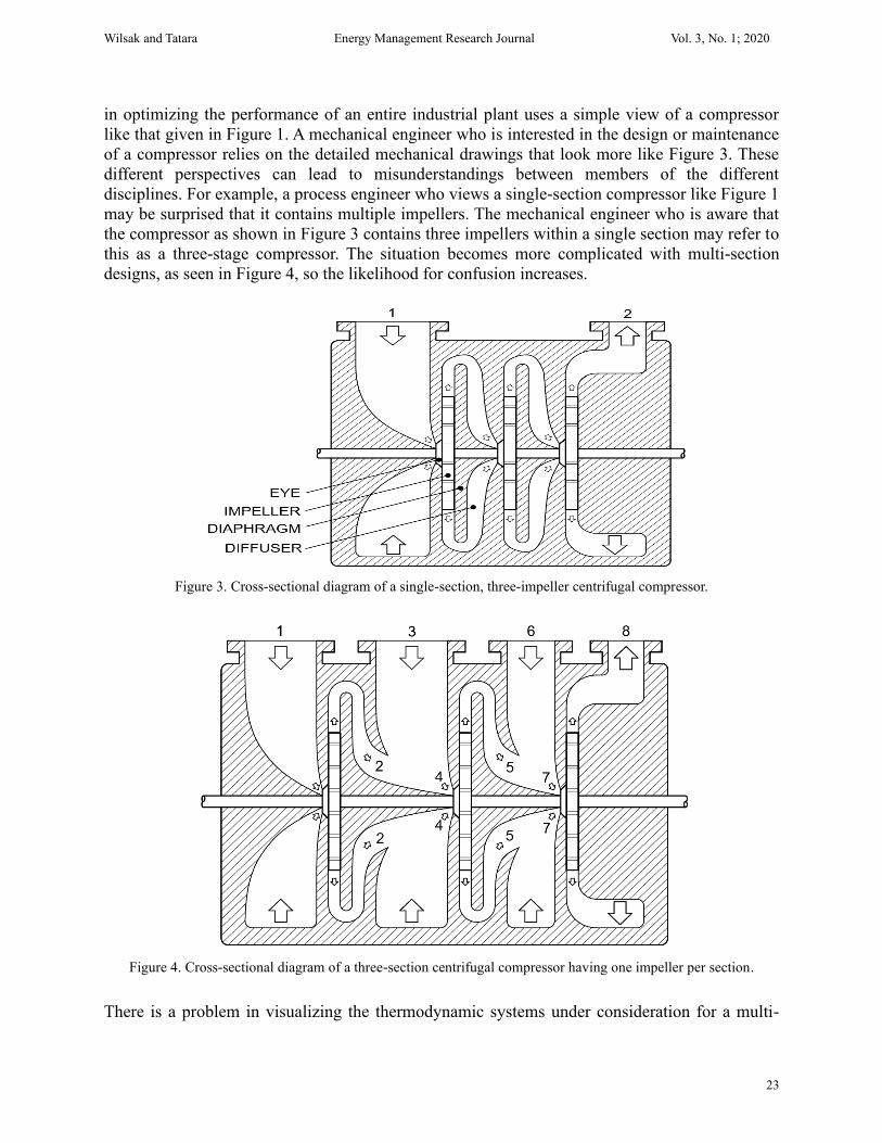
Figure 3 is a drawing of a single-section centrifugal compressor containing three impellers.

Comparing with the schematic given in Figure 1, we can equate positions 1 and 2 of Figure 1 to

the suction and discharge flanged nozzles in Figure 3, respectively. Figure 3 details the gas flow

through the compressor. The gas is directed from the inlet nozzle to the eye of the first impeller.

Since the impellers are attached to the shaft, they rotate at the same speed as the shaft. As the gas

flows through the first impeller, it is accelerated due to the shape and rotational speed of the

impeller. The gas reaches its maximum velocity as it exits the impeller and enters the diffuser.

The diffuser is designed to slow the gas before it is directed to the eye of the next impeller. As

the gas slows, some of its kinetic energy is converted into internal energy. This is manifested as a

change in gas temperature and pressure. This process is repeated through each of the impellers.

The diffuser of the last impeller directs the gas to the outlet nozzle. Note the parts of the casing

that lie between the impellers and define the shape of the diffusers. These are called diaphragms,

one of which is indicated in the figure.

One of the reasons that a thermodynamic analysis is so powerful is that it addresses energy

exchanges between a system and its surroundings rather than the intricacies of the phenomena

occurring within the system. While Figure 1 is sufficient for the derivation and application of the

thermodynamic equations for a single section polytropic compressor, Figure 3 provides more

detailed information of what occurs inside the compressor. A chemical engineer who is interested


23

in optimizing the performance of an entire industrial plant uses a simple view of a compressor

like that given in Figure 1. A mechanical engineer who is interested in the design or maintenance

of a compressor relies on the detailed mechanical drawings that look more like Figure 3. These

different perspectives can lead to misunderstandings between members of the different

disciplines. For example, a process engineer who views a single-section compressor like Figure 1

may be surprised that it contains multiple impellers. The mechanical engineer who is aware that

the compressor as shown in Figure 3 contains three impellers within a single section may refer to

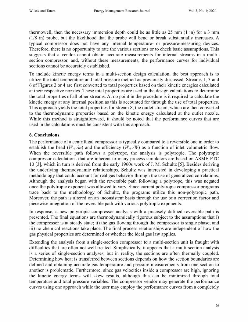
this as a three-stage compressor. The situation becomes more complicated with multi-section

designs, as seen in Figure 4, so the likelihood for confusion increases.

Figure 3. Cross-sectional diagram of a single-section, three-impeller centrifugal compressor.

Figure 4. Cross-sectional diagram of a three-section centrifugal compressor having one impeller per section.

There is a problem in visualizing the thermodynamic systems under consideration for a multi-


24

section compressor. Figure 4 is a drawing of a three-section compressor with each section

containing a single impeller and corresponds to the schematic given in Figure 2. In viewing

Figure 4, it is not obvious where the first section ends and the second begins.

When viewing the three sections of Figure 2, the intermediate streams seem well defined since it

is obvious how to choose the thermodynamic systems. To solve the problem illustrated by Figure

2, we need to consider five systems. These include the three compressors: i) from stream 1 to

stream 2; ii) from stream 4 to stream 5; and iii) from stream 7 to stream 8. The other two systems

involve the mixing of an impeller effluent with a side-stream -- specifically, the mixing of

streams 2 and 3 to obtain stream 4 and the mixing of streams 5 and 6 to obtain stream 7. It

appears reasonable to assume that the mixing operations occur adiabatically since Figure 2

implies that the mixing occurs at a well-defined point. However, when viewing Figure 4, it is not

at all obvious how to define the five systems unequivocally, and therefore the locations of the

internal streams are also poorly defined.

It is necessary to assign different parts of the casing to each of the thermodynamic systems in our

analysis in order to define the boundaries and therefore the location of the internal streams.

Figure 5 shows one way to define the second and third systems of this multi-section compressor.

Streams 2 and 3 enter the second system while stream 4 exits. Stream 4 enters the third system

while stream 5 exits. From Figure 5, it should be clear that the exact locations of streams 2, 4 and

5 are subjective, depending on the choice of the boundaries. When viewed from the perspective

of Figure 2, it seemed reasonable to assume that the mixing in the second system occurred

adiabatically. From the perspective of Figure 5, heat transfer must be considered as indicated.

Similar statements can be made about heat transfer into and out of the third system as depicted in

Figure 5, as well as the other three systems that have not been explicitly shown.

Figure 5. Cross-sectional diagram with heat flows and thermodynamic boundaries of a three-section compressor

with one impeller per section: (a) heat transfer = and (b) mass flow = .


25

The extent of any heat transfer may be estimated by first performing the calculations assuming

that no heat transfer occurs and then assessing the resulting temperature gradients. Consider, for

example, a common three-section propene refrigeration compressor. Assume that each of the five

systems is adiabatic and the inlet streams 1, 3 and 6 are at -34, -10 and 2°C (-29.2, 14.0 and

35.6°F), respectively. The internal streams 2, 4, 5 and 7 are calculated to be 2, -4, 42 and 35°C

(35.6, 24.8, 107.6 and 95.0°F), respectively, and outlet stream 8 is 92°C (197.6°F). Referring to

Figure 5, then it must be concluded that large temperature gradients exist within the compressor,

and, therefore, the initial adiabatic assumption is improper. The maximum gradient is 90°C

(162°F) between streams 8 and 6, which are separated by a metal diaphragm. Also note the

substantial gradients along the shaft, nearly 40°C (72°F) between streams 7 and 4.

If significant heat transfer does occur internally between the systems of a multi-section

compressor during vendor testing, is this amount identical to when the unit is operating in the

field? This is particularly important when a Type 2 test, as permitted by ASME PTC 10, is

performed. A Type 2 test is appropriate when it is not possible to replicate field conditions, which

can occur when the gas is toxic, flammable or corrosive or when temperatures are extreme (e.g.,

cryogenic). ASME PTC 10 does not explicitly address internal heat transfer between systems.

Furthermore, due to field parameter changes that occur naturally as a process is optimized, a

compressor may not be operating near its original design point. For example, in the situation

where the capacity of the compressor has been increased significantly, the compressor may be

operating close to choke, and the conditions of the inlet streams could be much different than

originally specified. This will likely alter the heat leakage between sections, and the same

performance curves may not be valid.

Quantifying the internal heat transfer is not easy due to the fact that the path of the gas between

sections is three-dimensional and represents a difficult heat transfer problem. However, CFD

software has evolved and is capable of simulating quite complex problems with accuracy. One

such attempt numerically modeled the heat transfer through the solid centrifugal compressor

components (casing and impeller) due to the temperature increase as air was compressed [11].

Among the findings is that the effect is quite small when the pressure ratio is under 5; at greater

ratios, the internal heat leakage becomes significant and will reduce the pressure ratio 7.5% at a

ratio of 11. No attempt was made to speculate whether this same level of reduction in discharge

pressure would occur with other gases or other conditions. However, this study does suggest that

one approach may be to run a series of simulations to compute the heat transferred between

sections for a variety of gases and operating conditions. The results could be correlated

empirically as a function of the compressor’s pressure ratio and/or total power.

Another obstacle is in obtaining accurate temperature measurements for the internal streams of a

compressor [12] as measurement error directly impacts polytropic efficiency. Gilarranz [13]

conducted an uncertainty analysis for compressing nitrogen or carbon dioxide test gases; it is

shown that just ±1°C (±1.8°F) variation in suction and discharge temperatures leads to a 2 to 3%

deviation in compressor efficiency. This effect is greater in low pressure ratio compressions. In

Figure 5, for example, it would be difficult to install a temperature probe to measure the

temperature at position 2 or any other of the internal streams. The goal is to locate a probe where

the gas temperature is approximately isothermal along the length of the probe. Since gas

properties are changing dramatically inside the compressor, such locations are not obvious. If a

thermowell were used, then an immersion depth equal to about ten times the diameter of the

thermowell is required, about 150 mm (6 in) for a standard industrial probe. Without a


26

thermowell, then the necessary immersion depth could be as little as 25 mm (1 in) for a 3 mm

(1/8 in) probe, but the likelihood that the probe will bend or break substantially increases. A

typical compressor does not have any internal temperature- or pressure-measuring devices.

Therefore, there is no opportunity to rate the various sections or to check basic assumptions. This

suggests that a vendor cannot obtain accurate measurements for internal streams in a multi-

section compressor, and, without these measurements, the performance curves for individual

sections cannot be accurately established.

To include kinetic energy terms in a multi-section design calculation, the best approach is to

utilize the total temperature and total pressure method as previously discussed. Streams 1, 3 and

6 of Figures 2 or 4 are first converted to total properties based on their kinetic energies calculated

at their respective nozzles. These total properties are used in the design calculations to determine

the total properties of all other streams. At no point in the procedure is it required to calculate the

kinetic energy at any internal position as this is accounted for through the use of total properties.

This approach yields the total properties for stream 8, the outlet stream, which are then converted

to the thermodynamic properties based on the kinetic energy calculated at the outlet nozzle.

While this method is straightforward, it should be noted that the performance curves that are

used in the calculations must be consistent with this approach.

6. Conclusions

The performance of a centrifugal compressor is typically compared to a reversible one in order to

establish the head (Wrev/m) and the efficiency (Wrev/W) as a function of inlet volumetric flow.

When the reversible path follows a polytrope, the analysis is polytropic. The polytropic

compressor calculations that are inherent to many process simulators are based on ASME PTC

10 [3], which in turn is derived from the early 1960s work of J. M. Schultz [5]. Besides deriving

the underlying thermodynamic relationships, Schultz was interested in developing a practical

methodology that could account for real gas behavior through the use of generalized correlations.

Although the analysis began with the reversible path following a polytrope, this was negated

once the polytropic exponent was allowed to vary. Since current polytropic compressor programs

trace back to the methodology of Schultz, the programs utilize this non-polytropic path.

Moreover, the path is altered on an inconsistent basis through the use of a correction factor and

piecewise integration of the reversible path with various polytropic exponents.

In response, a new polytropic compressor analysis with a precisely defined reversible path is

presented. The final equations are thermodynamically rigorous subject to the assumptions that i)

the compressor is at steady state; ii) the gas flowing through the compressor is single phase; and

iii) no chemical reactions take place. The final process relationships are independent of how the

gas physical properties are determined or whether the ideal gas law applies.

Extending the analysis from a single-section compressor to a multi-section unit is fraught with

difficulties that are often not well treated. Simplistically, it appears that a multi-section analysis

is a series of single-section analyses, but in reality, the sections are often thermally coupled.

Determining how heat is transferred between sections depends on how the section boundaries are

defined and obtaining accurate gas temperature and pressure measurements from one section to

another is problematic. Furthermore, since gas velocities inside a compressor are high, ignoring

the kinetic energy terms will skew results, although this can be minimized through total

temperature and total pressure variables. The compressor vendor may generate the performance

curves using one approach while the user may employ the performance curves from a completely


27

different point of view. This leads to biases in the predictions. Furthermore, process changes in

the operating unit may alter the heat transfer between compressor sections, e.g., a warmer or

colder side-stream than in the original design may affect the original performance curves. In fact,

many commercial compressors are situated outdoors so heat transfer with the surroundings will

vary with changes in weather. All these issues increase the uncertainty in plant optimization or

debottlenecking simulations.

While the focus of this work is to improve the understanding of the underlying thermodynamic

process relationships in ASME PTC 10, it should be noted that the method by which physical

properties of the gas are calculated will impact the final results. Therefore, it is important that the

same physical properties model that was used in developing the performance curves by the

vendor is also employed by the user. Presumably, the physical properties model accurately

represents the behavior of the gas employed -- otherwise the results will be systematically

biased. It is best if vendor test data and physical properties models can be shared so that the user

can reproduce identical performance curves.

7. Acknowledgments

Mr. Buck Comstock drew Figures 1 through 5 to illustrate the concepts discussed in the text. We

appreciate his generous contributions.

References

[1] U. S. Energy Information Administration Reports. Data: State Electricity Profiles, Retrieved from

http://www.eia.gov, 2019.

[2] S. Li and F. Li, Prediction of cracking gas compressor performance and its application in process

optimization, Chinese Journal of Chemical Engineering, vol 20(6), pp. 1089-1093, 2012.

[3] Performance Test Code on Compressors and Exhausters (ASME PTC 10-1997), The American

Society of Mechanical Engineers, New York, NY, USA, 1998.

[4] M. R. Sandberg and G. M. Colby, Limitations of ASME PTC 10 in accurately evaluating centrifugal

compressor thermodynamic performance, Proceedings of the Forty-Second Turbomachinery

Symposium, Houston, TX, USA, October 1-3, 2013.

[5] J. M. Schultz, The polytropic analysis of centrifugal compressors, Journal of Engineering for Power,

vol 84(1), pp. 69-82, 1962.

[6] B. F. Evans and S. R. Huble, Centrifugal compressor polytropic performance: consistently accurate

results from improved real gas calculations, ASME Turbo Expo 2017: Turbomachinery Technical

Conference and Exposition, Charlotte, NC, USA, June 26-30, 2017.

[7] M. Taher, ASME PTC-10 performance testing of centrifugal compressors - the real gas calculation

method, SME Turbo Expo 2014: Turbine Technical Conference and Exposition, Dusseldorf,

Germany, June 16-20, 2014.

[8] M. Taher, Performance testing of centrifugal compressors - Schultz compressibility factors, ASME

Turbo Expo 2015: Turbine Technical Conference and Exposition, Montreal, Canada, June 15-19,

2015.

[9] M. Taher, ASME PTC-10 and heat capacity relations for polytropic and isentropic compression

process of real gas, ASME Turbo Expo 2017: Turbomachinery Technical Conference and Exposition,

Charlotte, NC, USA, June 26-30, 2017.

[10] J. H. Park, Y. Shin and J. T. Chung, Performance prediction of centrifugal compressor for drop-in


28

testing using low global warming potential alternative refrigerants and performance test codes,

Energies, vol 10(12), pp. 1-21, 2017.

[11] S.M. Moosania and X. Zheng, Effect of internal heat leakage on the performance of a high-pressure

ratio centrifugal compressor, Applied Thermal Engineering, vol 111, pp. 317-324, 2017.

[12] D. Fiaschi, G. Manfrida and L. Tapinassi, Improving the accuracy of tests for centrifugal compressor

stage performance prediction, 8th Biennial ASME Conference on Engineering Systems Design and

Analysis, Torino, Italy, July 4-7, 2006.

[13] J. L. Gilarranz, Uncertainty analysis of a polytropic compression process and application to

centrifugal compressor performance testing, ASME Turbo Expo 2005: Power for Land, Sea and Air,

Reno- Tahoe, NV, USA, June 6-9, 2005.

Biographical information

Dr. Richard Wilsak earned a PhD in

Chemical Engineering from Northwestern

University in 1986. He retired after working

as a Research Engineer at Amoco Chemical

Company and BP for 29 years. There he

improved olefins and paraxylene processes

while obtaining 10 patents and 12

publications.

Prof. Robert Tatara holds a PhD in

Chemical Engineering and is with the

Department of Engineering Technology,

Northern Illinois University, DeKalb, IL,

USA. He has taught courses in energy

management, heat transfer, and thermal

design. His research interests include heat

exchangers, biofuels, and sustainable

polymeric materials.

Documents

Reassessing Polytropic Compressor Calculations of ASME PTC 10