IZA DP No. 3205

The Peter Principle: An Experiment

David L. DickinsonMarie Claire Villeval

DI

SC

US

SI

ON

PA

PE

R S

ER

IE

S

Forschungsinstitutzur Zukunft der ArbeitInstitute for the Studyof Labor

December 2007

The Peter Principle: An Experiment

David L. Dickinson Appalachian State University

Marie Claire Villeval

CNRS-GATE, University of Lyon and IZA

Discussion Paper No. 3205 December 2007

IZA

P.O. Box 7240 53072 Bonn

Germany

Phone: +49-228-3894-0 Fax: +49-228-3894-180

E-mail: iza@iza.org

Any opinions expressed here are those of the author(s) and not those of the institute. Research disseminated by IZA may include views on policy, but the institute itself takes no institutional policy positions. The Institute for the Study of Labor (IZA) in Bonn is a local and virtual international research center and a place of communication between science, politics and business. IZA is an independent nonprofit company supported by Deutsche Post World Net. The center is associated with the University of Bonn and offers a stimulating research environment through its research networks, research support, and visitors and doctoral programs. IZA engages in (i) original and internationally competitive research in all fields of labor economics, (ii) development of policy concepts, and (iii) dissemination of research results and concepts to the interested public. IZA Discussion Papers often represent preliminary work and are circulated to encourage discussion. Citation of such a paper should account for its provisional character. A revised version may be available directly from the author.

IZA Discussion Paper No. 3205 December 2007

ABSTRACT

The Peter Principle: An Experiment*

The Peter Principle states that, after a promotion, the observed output of promoted employees tends to fall. Lazear (2004) models this principle as resulting from a regression to the mean of the transitory component of ability. Our experiment reproduces this model in the laboratory by means of various treatments in which we alter the variance of the transitory ability. We also compare the efficiency of an exogenous promotion standard with a treatment where subjects self-select their task. Our evidence confirms the Peter Principle when the variance of the transitory ability is large. In most cases, the efficiency of job allocation is higher when using a promotion rule than when employees are allowed to self-select their task. This is likely due to subjects’ bias regarding their transitory ability. Naïve thinking, more than optimism/pessimism bias, may explain why subjects do not distort their effort prior to promotion, contrary to Lazear’s (2004) prediction. JEL Classification: C91, J24, J33, M51, M52 Keywords: promotion, Peter Principle, sorting, experiment Corresponding author: Marie-Claire Villeval CNRS-GATE 93, Chemin des Mouilles 69130 Ecully France E-mail: villeval@gate.cnrs.fr

* Valuable comments were provided by Peter Groothuis and participants at the Economic Science Association world meetings in Rome and at the conference of the European Association of Labour Economists in Oslo. Funding from a grant from the ACI-INTERSHS program at the French Ministry of Research and from the Walker College of Business at Appalachian State University is gratefully acknowledged.

1

1. INTRODUCTION

The Peter Principle states that in any hierarchical organization, employees tend to

rise to their level of incompetence (Peter and Hull, 1969). Lazear (2004) provides a

theoretical model showing that the Peter Principle is a necessary consequence of any

promotion rule when outcomes are a function of both a permanent and transitory (i.e.,

random) ability component. When job-specific transitory ability has expected value equal

to zero, those promoted most likely had a favorable “random draw” prior to promotion. A

regression-to-the-mean effect drives the Peter Principle, resulting in job allocation

inefficiency. While apparently akin to adverse selection, a key difference is that the agents

themselves (i.e., workers) can be worse off with incentive compatible wages. Thus, it can

be in the interests of both principal and agents to avoid this type of inefficient job sorting.

Peter and Hull (1968) and Lazear (2004) provide a variety of real-world examples

of the Peter Principle: the decline of faculty productivity after tenure, the lower quality of

movie sequels, a relatively less satisfying second experience at a new restaurant. Using

data from a large hierarchical British financial sector firm, Barmby et al. (2006) find some

evidence that performance declines after promotion. Two-thirds of the fall in post-

promotion performance is attributed to the Peter Principle and one third to reduced

incentives. We know of no other empirical tests of the Peter Principle, largely due to

selection bias when employees are mobile and the difficulty in measuring “luck”.1 The

laboratory offers a distinct advantage in this instance. The aim of this paper is to provide

an experimental test of the Peter Principle and to measure its robustness to various

manipulations of the promotion rule.

1 In Barmby et al. (2006), the importance of luck is proxied by a logit model of promotion depending on the distance between the evaluation rating of the individual and the average rating of his current grade.

2

In our experiment, agents perform a real effort task, with observable outcome

determined by ability and transitory (i.e., random) components. If output reaches a

standard, the agent is promoted to a more difficult task in the second production stage. The

wage profiles of the easy and difficult tasks are such that high ability agents would earn

more performing the hard task. Lazear (2004) predicts that the Peter Principle is a function

of the relative size of the transitory component, and so we implement three treatments that

manipulate the variance of the random term. In an additional treatment, we allow subjects

to self-select into the easy or difficult task in the second stage. This constitutes the core

contribution of this paper: a comparison of the job matching efficiency of self-selection

versus promotion rules. Indeed, Lazear's model predicts that if employees know their

permanent ability but firms do not, it is more efficient for employees to self-select their task

rather than use an exogenous promotion standard. Furthermore, since job mismatch

reduces worker payoffs, strategic effort distortion may result under a promotion rule,

because low (high) ability employees should strategically distort their effort downward

(upward) in the first stage to ensure efficient task assignment.

Our laboratory environment successfully recreates the Peter Principle, though only

when the variance of the transitory term is quite high. This is no only consistent with

Lazear (2004), but it also validates our experimental design. We next show that self-

selection into one’s task is not necessarily more efficient than promotions, except when the

variance of the transitory ability is large. This result may be due to subjects being

overconfident with respect to the likely draw of their transitory ability component, thus

inducing them to inefficiently self-select into the hard task. Lazear (2004) also

hypothesizes an effort distortion prior to promotion, as workers attempt to ensure

3

assignment to their optimal task. We find no evidence of effort distortion, contrary to

theoretical predictions. Because agent overconfidence does not appear connected to effort

choices (as opposed to job choice), this lack of effort distortion is more consistent with the

hypothesis that agents are naïve rather than strategic in this environment..

The reminder of this paper is organized as follows. Section 2 presents the

theoretical model. Section 3 develops the experimental design. Section 4 details the results

and Section 5 discusses these results and concludes.

2. THEORY

In this section, we present briefly the main characteristics and predictions of

Lazear's (2004) model. The firm’s productive activity consists of an easy (E) and a hard

(H) task. Every agent’s ability consists of a permanent component, A, and a transitory or

random component in period t,

�

!t, that is i.i.d. over time. The principal cannot observe

agents’ permanent ability, but only

�

ˆ A = A + !t.2 The agent’s productivity on the easy task

is:

�

YE

= ! + " A + #t( ) and on the hard task is: ( )

t

HAY !"# ++= , with

�

! > " and

�

! < " .

Thus, a less able agent will be more productive (i.e., have a comparative advantage) when

performing the easy task than when performing the hard task. Where these two

productivity profiles cross corresponds to the ability level at which the employer and

worker are both indifferent between being promoted or not, assuming incentive compatible

piece-rate pay for workers.

Consider the following two-stage game. In the first stage of the game, all agents are

assigned to the easy task. At the end of the first stage, the principal only observes  and

2 In Lazear (2004)’s general model, the agent is not better informed than the principal. He also considers the case of asymmetric information, which is what we consider given our interest in the self-selection question.

4

must decide on each agent’s task allocation for the second stage of the game. The principal

determines a standard, A*, such that if

�

ˆ A ! A * the agent is promoted to the hard task, and if

�

ˆ A < A * he again performs the easy task in the second stage.

Lazear’s model generates the prediction that, on average, the agents who are

promoted have a lower observable outcome after promotion—the Peter Principle. In more

formal terms, the conditional expected value of

�

!1 for those agents who have been

promoted is given by:

�

E !1A + !

1> A*( ) = E ! ! > A*"A( )

"#

#

$ f A( )dA , which is greater than

zero. In contrast, the expected value of

�

!2 is zero. As a consequence, there is a predicted

decrease in the expected observed ability of the promoted agents:

�

A + E !1A + !

1> A*( ) > A + E !

2A + !

1> A*( ). Another intuitive prediction of the model is

that the Peter Principle will be stronger when the transitory ability component is high

relative to one’s permanent ability component.3

An extension of the model introduces strategic agent behavior. When agents have

perfect information on their permanent ability, they can manipulate their effort to influence

their assignment to a specific task. Let

�

eE and

�

eH

denote the effort levels chosen by an

agent on the easy and hard tasks, respectively, with c(e) the associated cost incurred. Since

the expected value of the transitory component is 0, agents prefer the hard task if the

following holds: ! + " A + eE( ) # c eE( ) < $ + % A + e

H( ) # c eH( ) . The testable implication

is that, under a promotion rule, an agent will strategically distort his level of effort

downward (upward) if his permanent ability is low (high). Intuitively, the agent distorts

3 When transitory components exist, Lazear (2004) shows that promotion cutoffs will be adjusted to take into account the Peter Principal. Because we seek to examine agent behavior in this paper, we exogenously impose a promotion standard in our experiments rather than submit them to subject choice.

5

effort to influence assignment to the task in which he has the comparative advantage. In

such cases, allowing agents to self-select their task assignment should be more efficient

than a promotion rule.

To sum up, Lazear (2004) delivers several testable implications that we examine:

a) When observable output is a function of permanent and random ability components, average agent output will decrease (increase) following promotion (non-promotion).

b) The larger the random component relative to the permanent one, the stronger the Peter Principle (e.g., the larger the decrease in average post- promotion output).

c) If agents know their ability, then effort will be distorted downward (upward) by lower (higher) ability agents prior to a promotion stage. 4

d) If agents know their ability, allowing agents to self-select their second-stage task will be perfectly efficient and should be more efficient than a promotion tournament.

3. EXPERIMENTAL DESIGN

The game reproduces the main characteristics of Lazear’s (2004) model. Since our

main interest is in recreating the Peter Principle and examining agents' strategic behavior,

subjects are all assigned as agents. In promotion treatments, we use an exogenous standard.

The Task

The cognitive task utilized is a modified version of the task in Baddeley (1968).

The easy task involves reading a short sentence that describes the order of three letters.

The subjects have to type in these three letters in the order implied by the sentence. For

example, “S follows B, is not preceded by G” implies the order “BSG”.5 We mix passive

(e.g., “is followed by”) and active (e.g., “precedes”) statements, positive (e.g., “follows”)

4 In this framework, effort distortion is aimed at distorting job allocation. In the literature on promotions, there are many other types of distortion where the principals themselves manipulate information given to the agents or competitors (Meyer, 1991; Bernhardt, 1995). We do not consider these other sources of distortion. 5 Subjects are given a precise rule to use for lettering ordering, and with the rule there is a unique letter ordering for each sentence description (see instructions in Appendix B).

6

and negative statements (“does not precede”) across sentences. Sentences are randomly

generated from all letters of the alphabet. Once typed, the sentence is auto-checked against

the correct answer after each sentence, so that subjects can learn and improve more rapidly.

Though Baddeley (1968) indicates only minor learning with repetition of the task, we

consider learning as a potential confound in the data and implement a practice stage of both

easy and hard tasks. The hard task is similar except that each sentence contains five letters.

For example, “S follows B, is not preceded by G, precedes H, is not followed by J” implies

the ordering “JBSGH”. The advantage of this task is that no specific knowledge is needed,

difficulty can be increased by increasing the number of letters without altering the cognitive

focus of the task, and the outcome is easily measurable. Also, effort is distinguished from

ability by use of practice rounds, which contain no incentives to distort effort. Finally, our

Calibration treatment provides an added way to filter learning trends from the data.

Timing of the game and determination of the parameter values

We first utilize a distinct Calibration treatment to create wage profiles such that

high ability subjects would earn more in the hard task. Thus, this treatment generates data

on average subject ability on each task, which is also necessary to determine a cutoff point

for promotions. Because it involves several stages of performing the effort task, we also

use this treatment to filter the learning component from the data in the other treatments.

We use the same time structure in the Calibration treatment as in all other treatments.

A treatment consists of four stages. In stages 1 and 2, the subject performs the 3-

letter then 5-letter tasks during separate 7 minute periods.6 These first two stages provide

subjects information on their abilities for each task. In stage 3, the subject performs the 3- 6 In each of the first two stages, subjects practice the task three times as part of the instructions. During this practice phase subjects cannot proceed to the next sentence before providing a correct answer.

7

letter task again during 7 minutes. The number of correctly solved sentences in stage 3 is

our proxy for the subject’s ability, and the difference between stage 1 and stage 3 sentences

solved is the general learning trend. At the end of stage 3, the subject draws an i.i.d random

number from a uniform U[-12,+12] distribution. This random number corresponds to the

task-specific transitory component in the theoretical model. The subject’s “observable”

outcome in stage 3—the outcome on which payment is based—is the sum of the number of

correctly solved sentences and the random draw number.

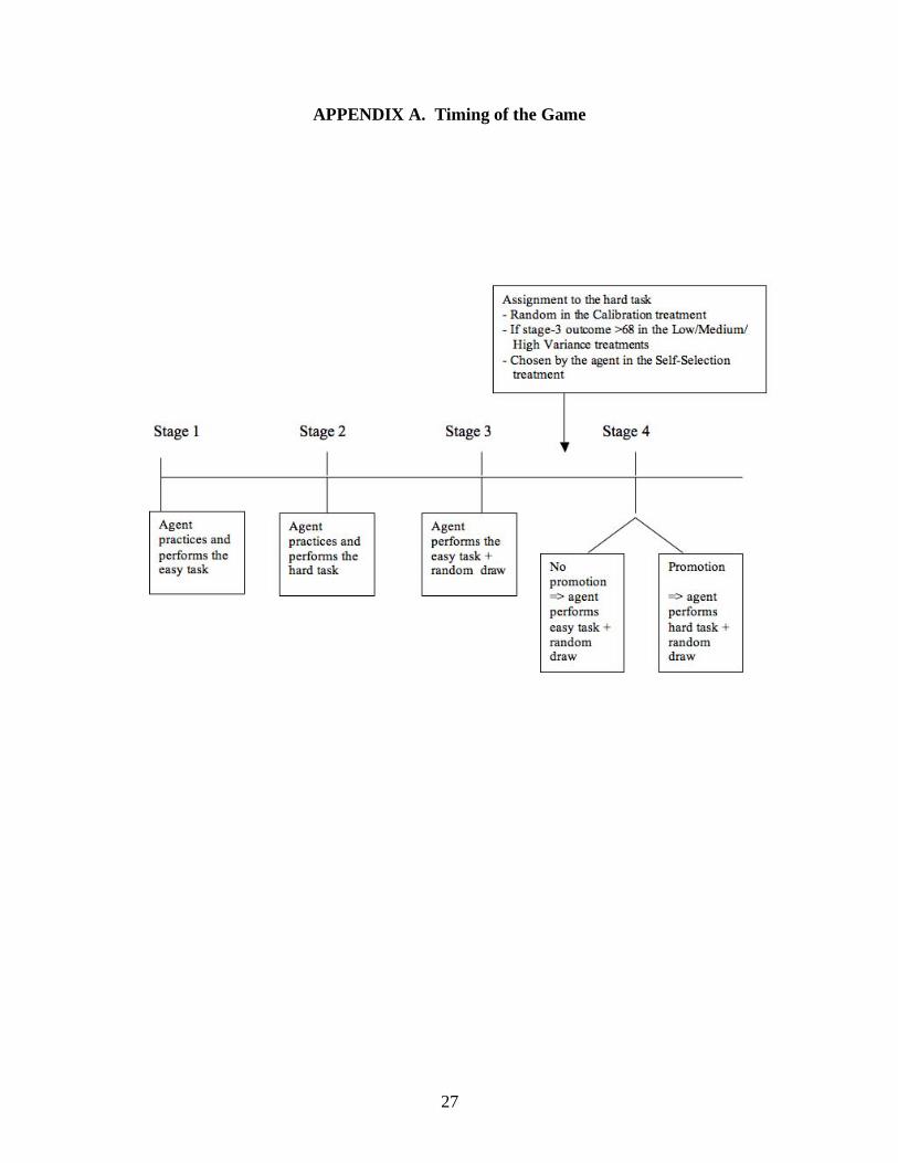
In stage 4, some subjects are assigned the easy task and others the hard task. In the

Calibration treatment, the assignment is purely random: half of the subjects are assigned to

each task. Those assigned to the easy task again solve 3-letter sentences during a 7-minute

period, after which a random draw from U[-12,+12] is added to the number of correct

sentences solved. Those assigned to the hard task solve 5-letter sentences during the same

7-minute period and then draw an i.i.d. random number from a uniform U[-4,+4]. The

difference in the support of the uniform distributions corresponds to the induced output

equivalent of easy to hard tasks: one hard sentence solved is considered as valuable to the

employer as three easy sentences. The subject’s stage 4 outcome is the sum of the number

of correct sentences and the random term. Appendix A summarizes the game’s timing.

The payoffs in each of the four stages have been determined as follows. Pilot

sessions gave us an informed estimate of average ability at each task: the average subject

solved 2.05 times as many 3-letter sentences (65) vs. 5-letter sentences (30). In order to

create the differing slopes of each task’s wage profile for the Calibration treatment, we first

induce an output equivalence of 3 easy task units to each 1 hard task unit. That is, subjects

are paid a piece rate that is 3 times as large for the hard task, corresponding to ! = 3" .

8

(Accordingly, as mentioned above, the variance of the random component in the easy task

is 3 times larger than in the hard task). By manipulating the piece-rates so that the hard

task is rewarded at a rate greater than the subjects’ observed opportunity cost of the hard

task, we effectively induce wage profiles of differing slopes.

Fixed payments are added in each stage of the Calibration treatment in order to

create the desired overlapping wage profiles. In stage 1, the subject receives a fixed

payment of 135 points and the piece-rate pays 3 points for each correct 3-letter sentence

solved (i.e., the easy task). In stage 2, the fixed payment is 9 points and each correct 5-

letter sentence (i.e., hard task) is paid a piece-rate of 9 points. In stage 3, the easy task is

again performed with pay structure as in stage 1, while subjects are randomly assigned to

either the hard or easy task, with the corresponding pay structure, in stage 4. The

Calibration treatment allows us to adjust the values of the parameters, examine learning

trends, and to determine the promotion cut-off point in the Promotion treatments.

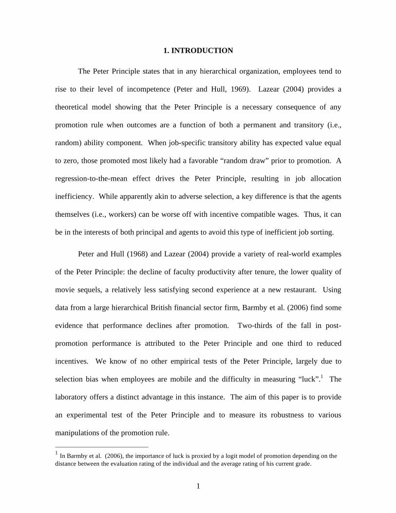
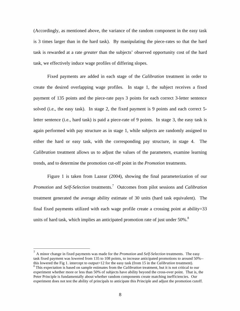
Figure 1 is taken from Lazear (2004), showing the final parameterization of our

Promotion and Self-Selection treatments.7 Outcomes from pilot sessions and Calibration

treatment generated the average ability estimate of 30 units (hard task equivalent). The

final fixed payments utilized with each wage profile create a crossing point at ability=33

units of hard task, which implies an anticipated promotion rate of just under 50%.8

7 A minor change in fixed payments was made for the Promotion and Self-Selection treatments. The easy task fixed payment was lowered from 135 to 108 points, to increase anticipated promotions to around 50%--this lowered the Fig 1. intercept to output=12 for the easy task (from 15 in the Calibration treatment). 8 This expectation is based on sample estimates from the Calibration treatment, but it is not critical to our experiment whether more or less than 50% of subjects have ability beyond the cross-over point. That is, the Peter Principle is fundamentally about whether random components create matching inefficiencies. Our experiment does not test the ability of principals to anticipate this Principle and adjust the promotion cutoff.

9

Figure 1. Productivity and cut-off point

The Treatments

We have tested four treatments besides the Calibration treatment: the Promotion-

σLow, Promotion-σMedium, Promotion-σHigh treatments, and the Self-Selection treatments.

The Promotion-σLow treatment constitutes the benchmark of this game. As in the

Calibration treatment, Promotion-σLow utilizes a random component distributed uniformly

on the interval [-12,+12] in the easy task and on the interval [-4,+4] in the hard task.

In contrast with the Calibration treatment in which promotion after stage 3 was

random, promotion in Promotion-σLow is based on the comparison between the individual’s

outcome and a promotion standard. The promotion standard is set to 68 easy task units of

output, approximately corresponding to the Fig. 1 cross-over point of output=33 units of

hard task.9 The Promotion-σLow treatment is a baseline aimed at recreating the basic Peter

9 Recall that this easy-hard task correspondence was from the pilot sessions, where average easy task output was 2.05 times that of the hard task output, or (2.05)*33≈68. The analogous correspondence in the Calibration treatment stages 3 and 4 was that average easy task output was 2.0 times that of the hard task. It is important to realize that we cannot use stages 1 and 2 to generate a hard-to-easy task conversion rate for each individual subject because of the learning confound in those data.

10

Principle, and its relation to the relative size of the transitory ability component is examined

by implementing Promotion-σMedium and Promotion-σHigh. In Promotion-σMedium, the

random component is distributed uniformly on the interval [-24,+24] and [-8,+8] in the easy

and hard tasks, respectively. In Promotion-σHigh, it is distributed uniformly [-75,+75] and

[-25,+25] in the easy and hard tasks, respectively. The testable theoretical implication is

that the Peter Principle will be strongest in Promotion-σHigh and weakest in Promotion-

σLow. A comparison of stage 3 outcomes in the Promotion and Calibration treatments

allows us to examine the hypothesis that subjects distort effort in anticipation of promotion.

In the Self-Selection treatment, the random ability component is distributed as in

Promotion-σLow, but the subject chooses her stage 4 task. It is reasonable to assume that

she has some knowledge of her ability on each task from the previous stages, and so we

assume self-selection should be efficient. The comparison of outcomes in stage 4 of the

Promotion and Self-Selection treatments provides an efficiency comparison of exogenous

promotion standards versus self-selection for job sorting.

Finally, in the Calibration and Promotion treatments, a hypothetical response of

preferred stage 4 task is elicited at the beginning of this stage. It was made clear to subjects

that their task had already been determined and the hypothetical response would have no

bearing on their stage 4 task. Nevertheless, this response may provide some indication of

whether subjects correctly assessed their abilities. Treatment details are shown in Table 1.

11

Table 1. Main treatment characteristics

Treatment Assignment to Hard task

Variance On Easy task

Variance on Hard task

# of sessions

# of subjects

Calibration Promotion-σLow Promotion-σMedium Promotion-σHigh Self-Selection

Random Standard Standard Standard

Self-Selection

U[-12,+12] U[-12,+12] U[-24,+24] U[-75,+75] U[-12,+12]

U[-4,+4] U[-4,+4] U[-8,+8]

U[-25,+25] U[-4,+4]

2 2 2 2 2

38 37 38 37 40

Experimental Procedures

Ten sessions were conducted at the Groupe d’Analyse et de Théorie Economique

(GATE), Lyon, France, with 2 sessions per treatment. 190 undergraduate subjects were

recruited from local Engineering and Business schools. 81.05% of the subjects had never

participated in an experiment. On average, a session lasted 60 minutes. The experiment

was computerized using the REGATE program (Zeiliger, 2000). Upon arrival, the subjects

were randomly assigned to a computer terminal, and experimental instructions for the first

stage of the game (see Appendix B) were distributed and read aloud. Questions were

answered privately. Subjects then practiced the easy task with 3 sentences without payment

until they were correctly solved, after which point the 7-minute paid easy task started. At

the end of the 7 minutes, we distributed the instructions for the second stage of the game

and answered to the participants’ questions. Once the practice and 7-minute hard task have

been performed, the instructions for both stage 3 and stage 4 were distributed together and

read aloud. Knowing the rules for task assignment in stage 4 before starting stage 3

allowed subjects to behave strategically in Stage 3, if desired, in the Promotion treatments.

After stage 3, subjects were given a brief 3-minute break, with no communication allowed.

We used a conversion rate of 100 points for each Euro. At the end of each session, payoffs

12

were totaled for the four stages. In addition, the participants received €4 as a show-up fee.

The average payoff was €15.40, and subjects were each paid in private in a separate room.

4. RESULTS

The Peter Principle

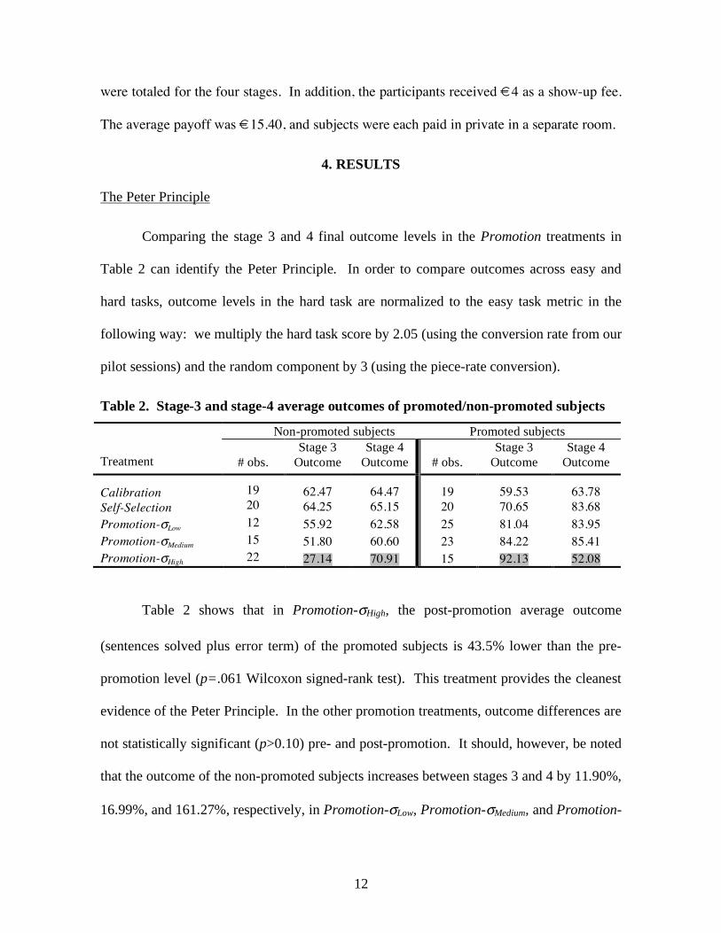
Comparing the stage 3 and 4 final outcome levels in the Promotion treatments in

Table 2 can identify the Peter Principle. In order to compare outcomes across easy and

hard tasks, outcome levels in the hard task are normalized to the easy task metric in the

following way: we multiply the hard task score by 2.05 (using the conversion rate from our

pilot sessions) and the random component by 3 (using the piece-rate conversion).

Table 2. Stage-3 and stage-4 average outcomes of promoted/non-promoted subjects

Non-promoted subjects Promoted subjects Treatment

# obs.

Stage 3 Outcome

Stage 4 Outcome

# obs.

Stage 3 Outcome

Stage 4 Outcome

Calibration Self-Selection Promotion-σLow

Promotion-σMedium Promotion-σHigh

19 20 12 15 22

62.47 64.25 55.92 51.80 27.14

64.47 65.15 62.58 60.60 70.91

19 20 25 23 15

59.53 70.65 81.04 84.22 92.13

63.78 83.68 83.95 85.41 52.08

Table 2 shows that in Promotion-σHigh, the post-promotion average outcome

(sentences solved plus error term) of the promoted subjects is 43.5% lower than the pre-

promotion level (p=.061 Wilcoxon signed-rank test). This treatment provides the cleanest

evidence of the Peter Principle. In the other promotion treatments, outcome differences are

not statistically significant (p>0.10) pre- and post-promotion. It should, however, be noted

that the outcome of the non-promoted subjects increases between stages 3 and 4 by 11.90%,

16.99%, and 161.27%, respectively, in Promotion-σLow, Promotion-σMedium, and Promotion-

13

σHigh, which is another implication of the Peter Principle. These differences are all

statistically significant (p=0.091, p=0.073, and p=0.001, respectively).

The existence of the Peter Principle is related to the existence of a transitory ability

component. As predicted, luck plays a greater role in promotion in the Promotion

treatments. In Promotion-σLow , 72% of the promoted subjects had a positive transitory

component in stage 3, compared to only 42% of the non-promoted subjects (Mann-

Whitney, p=.079). In Promotion-σMedium , the respective percentages are 74% and 33.%

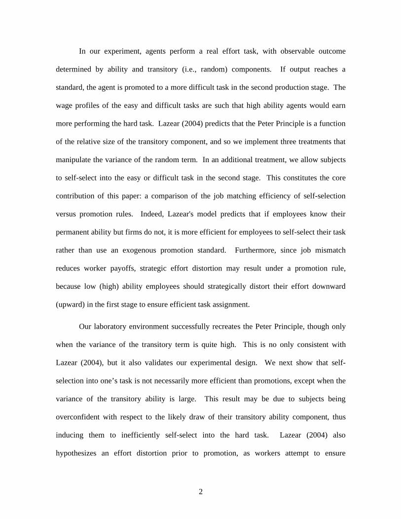
(p=0.014) and in Promotion-σHigh , 80% and 9% (p<0.001). Figure 2 displays the average

random term drawn in stage 3 for each treatment, sorting subjects according to whether

they are promoted or not in stage 4.

Figure 2. Average stage 3 transitory ability sorted by task in stage 4

Figure 2 confirms that in most Promotion treatments, the promoted subjects (labeled

‘Hard 4’) have been luckier than the non-promoted ones, whereas in the Calibration

14

treatment the difference is not significant. Their average transitory ability is positive and it

increases in its variance. Non-promoted subjects have a negative average transitory ability.

According to Mann-Whitney tests, the differences in average transitory components

between promoted and non-promoted subjects are significant in Promotion-σLow (p=0.011)

and Promotion-σHigh (p<0.001), while marginally insignificant in Promotion-σMedium

(p=0.120). As expected, stage 4 outcomes reflect a reversion-to-mean effect of the

transitory component, which completes the Peter Principle.

By next examining the agents’ abilities, we can analyze promotion mistakes (i.e.,

inefficient allocations). Table 3 indicates the stage 3 permanent (i.e., non-transitory) ability

of promoted and non-promoted subjects by treatment. Then, it gives the numbers and

proportions of subjects who were wrongly promoted despite ability lower than 68 (“mistake

1”), the unlucky subjects who should have been promoted (“mistake 2”), and the subjects

who were efficiently allocated in stage 4.

Table 3. Stage 3 ability of promoted/non-promoted subjects and assignment mistakes

Stage 3-average ability Number of mistakes (percentages)

Treatment Non-

promoted Promoted Mistake 1

(promotion) Mistake 2

(no-promotion) Correct

decisions Calibration 59.95 58.68 12 (31.58) 5 (13.16) 21 (55.26) Self-Selection 61.7 72.35 9 (22.50) 6 (15.00) 25 (62.50) Promotion-σLow 57.33 77.32 2 (5.41) 1 (2.7) 34 (91.89) Promotion-σMedium 52.67 79.17 4 (10.53) 3 (7.89) 31 (81.58) Promotion-σHigh 60.68 60.60 11 (29.73) 10 (27.03) 16 (43.24)

If permanent ability were observable, only those subjects solving at least 68

sentences in stage 3 would be promoted. We observe that in the Promotion-σHigh treatment,

the average score of the promoted subjects in stage 3 is not significantly different from that

15

of the non-promoted subjects (Mann-Whitney test, p>0.10). In addition, it is significantly

lower than the promotion standard of 68 (t-test, p=0.057). Thus, a fraction of the subjects

are inefficiently promoted. Table 3 also indicates that mistake frequency increases in

transitory ability variance. As a whole, the Promotion treatments data (Tables 2, 3, Figure

2) result from a framework created to generate the principle, so these results are perhaps not

surprising. They are, however, an important validation of a rather complex experimental

design. We can therefore explore comparison institutions and their predicted effects on

effort distortion and self-selection—two key outcome variables not amenable to simulation.

Self-selection vs. Promotions

Our Self-Selection treatment allows us to test the hypothesis that one can escape the

Peter Principle by letting the individuals select their task. In Self-Selection, subjects who

chose the hard task in stage 4 increased normalized outcomes by a significant 18.44%

relative to stage 3 (p<0.001) (Table 2). This is partly due to a higher rate of negative

transitory components in stage 3 (Fig. 2). In contrast, those who chose the easy task only

increased their outcome by an insignificant 1.40% (Table 2, p>0.10). This stands in

contrast to the clearly observed Peter Principle in Promotion-σHigh.

The lack of Peter Principle in the Self-Selection treatment does not, however, imply

that decisions in that treatment are more efficient than with promotion standards. Table 3

indicates that, in Self-Selection, 22.50% chose the hard task in stage 4 although their score

in stage 3 was below 68, and 15.00% of the subjects made the opposite mistake. The

respective proportions of mistakes were 5.41% and 2.70% in Promotion-σLow, which has a

comparable transitory variance, and the differences are significant (Mann-Whitney tests,

p=0.031 and p=0.017, respectively). In addition, the size of the average error is larger in

16

the Self-Selection treatment than in the Promotion-σLow, treatment. Indeed, the average type

1-mistake amounts to 9.11 and the average type 2-mistake 8.33 in the Self-Selection

treatment; the respective values for the Promotion-σLow, treatment are 7.50 and 6.00. This

casts some doubts on the overall efficiency of self-selection and calls for further

comparative analysis of these two job allocation mechanisms.

In particular, we compare the efficiency of promotions, self-selection, and an ad hoc

random task assignment. If the proportion of subjects actually promoted in the data for a

treatment is x, then we simulated random promotion by randomly selecting x subjects to be

promoted. Therefore, simulated random assignment promotes the same number of subjects

as in the data, but not necessarily the same individuals. Efficiency is calculated as the

proportion of correct promotions (i.e. promotion when permanent ability is at least 68).10

We find that a promotion standard is generally more efficient than a random task

assignment. In Promotion-σLow , the efficiency rate is 92% vs. 54% with a random

assignment, while in Promotion-σMedium , the respective percentages are 82% and 76%.

When the variance of the transitory component is high, however, random assignment can

be more efficient than the promotion rule (due to the large Peter Principle at work). Indeed,

the efficiency rate is 43% in Promotion-σHigh and 54% with the simulated random

assignments. Self-Selection efficiency is 63%, which is more efficient than the simulated

random assignment of 45% in that same treatment. So, while self-selection efficiency is

higher than with random task assignment, our results do not support the prediction that task

allocations are uniformly more efficient with self-selection rather than promotion standards.

10 Note that this type of random assignment is distinct from just flipping a coin to determine stage 4 task assignments, as that method necessarily generates a 50% random promotion rate.

17

This conclusion is also confirmed by the analysis of hypothetical choices. In our

Promotion treatments, we asked subjects to make a hypothetical choice at the end of stage 3

about which task they would prefer in stage 4. Comparing these hypothetical choices with

the actual scores in stage 3 allows us to determine whether the subjects were biased in their

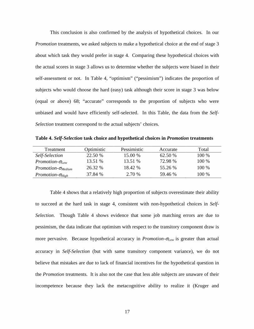
self-assessment or not. In Table 4, “optimism” (“pessimism”) indicates the proportion of

subjects who would choose the hard (easy) task although their score in stage 3 was below

(equal or above) 68; “accurate” corresponds to the proportion of subjects who were

unbiased and would have efficiently self-selected. In this Table, the data from the Self-

Selection treatment correspond to the actual subjects’ choices.

Table 4. Self-Selection task choice and hypothetical choices in Promotion treatments

Treatment Optimistic Pessimistic Accurate Total Self-Selection 22.50 % 15.00 % 62.50 % 100 % Promotion-σLow 13.51 % 13.51 % 72.98 % 100 % Promotion-σMedium 26.32 % 18.42 % 55.26 % 100 % Promotion-σHigh 37.84 % 2.70 % 59.46 % 100 %

Table 4 shows that a relatively high proportion of subjects overestimate their ability

to succeed at the hard task in stage 4, consistent with non-hypothetical choices in Self-

Selection. Though Table 4 shows evidence that some job matching errors are due to

pessimism, the data indicate that optimism with respect to the transitory component draw is

more pervasive. Because hypothetical accuracy in Promotion-σLow is greater than actual

accuracy in Self-Selection (but with same transitory component variance), we do not

believe that mistakes are due to lack of financial incentives for the hypothetical question in

the Promotion treatments. It is also not the case that less able subjects are unaware of their

incompetence because they lack the metacognitive ability to realize it (Kruger and

18

Dunning, 1999). Indeed, the subjects are informed about their score before they draw their

transitory ability component. Therefore, these mistakes are likely attributable to a biased

perception of the random ability component. Interestingly, the proportion of optimistic

choices increases with the variance of the transitory component, but not that of pessimistic

choices. In Promotion-σHigh, 38% of the subjects would have chosen the hard task although

their score was below 68, whereas this proportion is only 14% in Promotion-σLow

(Wilcoxon test: p=0.039).

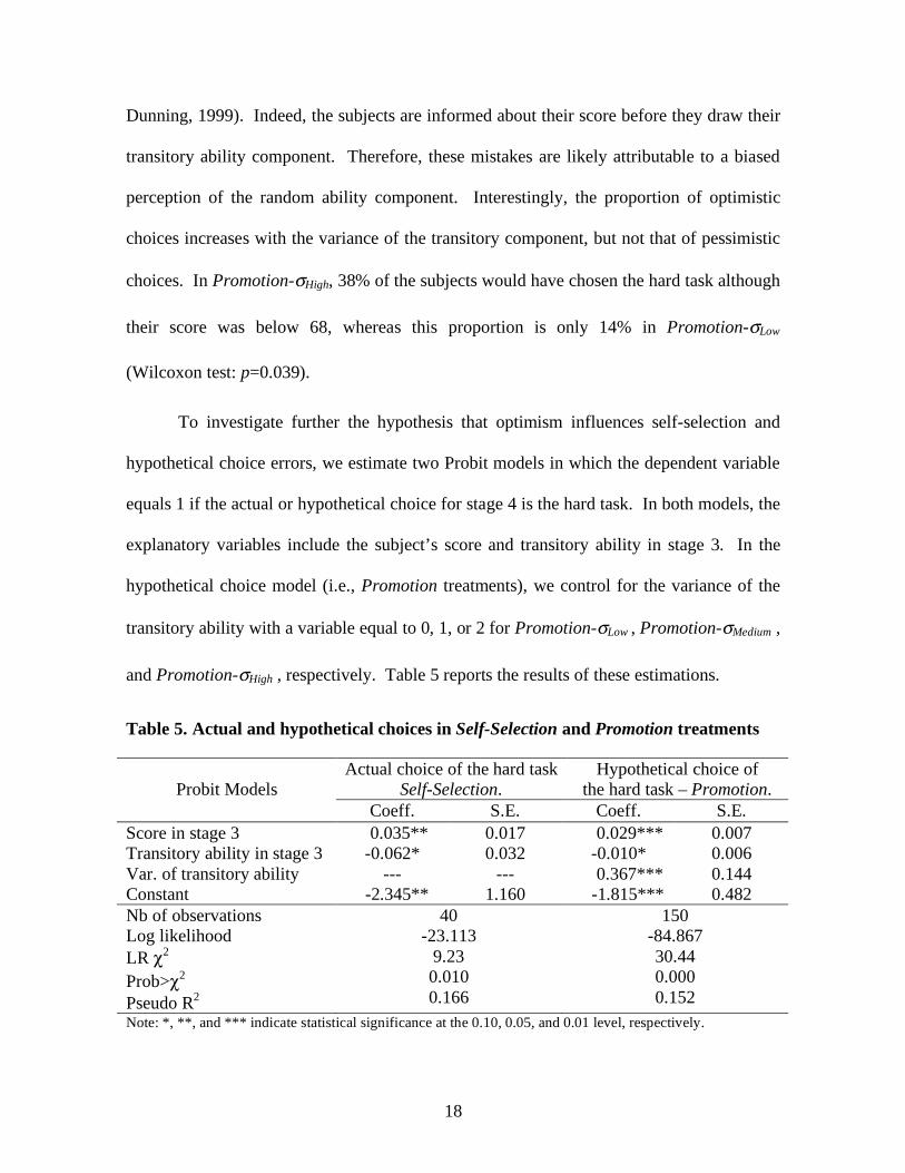
To investigate further the hypothesis that optimism influences self-selection and

hypothetical choice errors, we estimate two Probit models in which the dependent variable

equals 1 if the actual or hypothetical choice for stage 4 is the hard task. In both models, the

explanatory variables include the subject’s score and transitory ability in stage 3. In the

hypothetical choice model (i.e., Promotion treatments), we control for the variance of the

transitory ability with a variable equal to 0, 1, or 2 for Promotion-σLow , Promotion-σMedium ,

and Promotion-σHigh , respectively. Table 5 reports the results of these estimations.

Table 5. Actual and hypothetical choices in Self-Selection and Promotion treatments

Probit Models

Actual choice of the hard task Self-Selection.

Hypothetical choice of the hard task – Promotion.

Coeff. S.E. Coeff. S.E. Score in stage 3 Transitory ability in stage 3 Var. of transitory ability Constant

0.035** -0.062*

--- -2.345**

0.017 0.032

--- 1.160

0.029*** -0.010*

0.367*** -1.815***

0.007 0.006 0.144 0.482

Nb of observations Log likelihood LR χ2 Prob>χ2 Pseudo R2

40 -23.113

9.23 0.010 0.166

150 -84.867 30.44 0.000 0.152

Note: *, **, and *** indicate statistical significance at the 0.10, 0.05, and 0.01 level, respectively.

19

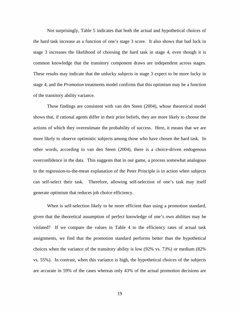
Not surprisingly, Table 5 indicates that both the actual and hypothetical choices of

the hard task increase as a function of one’s stage 3 score. It also shows that bad luck in

stage 3 increases the likelihood of choosing the hard task in stage 4, even though it is

common knowledge that the transitory component draws are independent across stages.

These results may indicate that the unlucky subjects in stage 3 expect to be more lucky in

stage 4, and the Promotion treatments model confirms that this optimism may be a function

of the transitory ability variance.

These findings are consistent with van den Steen (2004), whose theoretical model

shows that, if rational agents differ in their prior beliefs, they are more likely to choose the

actions of which they overestimate the probability of success. Here, it means that we are

more likely to observe optimistic subjects among those who have chosen the hard task. In

other words, according to van den Steen (2004), there is a choice-driven endogenous

overconfidence in the data. This suggests that in our game, a process somewhat analogous

to the regression-to-the-mean explanation of the Peter Principle is in action when subjects

can self-select their task. Therefore, allowing self-selection of one’s task may itself

generate optimism that reduces job choice efficiency.

When is self-selection likely to be more efficient than using a promotion standard,

given that the theoretical assumption of perfect knowledge of one’s own abilities may be

violated? If we compare the values in Table 4 to the efficiency rates of actual task

assignments, we find that the promotion standard performs better than the hypothetical

choices when the variance of the transitory ability is low (92% vs. 73%) or medium (82%

vs. 55%). In contrast, when this variance is high, the hypothetical choices of the subjects

are accurate in 59% of the cases whereas only 43% of the actual promotion decisions are

20

accurate (Wilcoxon test: p=0.010); the 54% efficiency rate with simulated assignment was

also lower than with hypothetical choices. We conclude that when the transitory

component variance is large relative to permanent ability,11 it is more efficient to allow

self-selection of task assignment rather than use promotions, even though the self-selection

choice may generate optimism.

It should be however noted that even in Promotion-σHigh , it might remain profitable

to use promotion standards. Indeed, the decrease in the total outcome of the promoted

subjects is compensated by the increase in outcome of the non-promoted ones.12

Furthermore, the average actual ability of the promoted subjects in stage 4 (68.88) is not

significantly different from the standard of 68 (t-test, p>0.10). One might hypothesize that

the promotion of low-ability agents provides an extra effort incentive to justify the

promotion.13 As we will see next, we can rule out this interpretation in our data. If one

considers all the Promotion treatments together, we observe that the subjects who have

been promoted by mistake increase on average their (normalized) score by 9.61% from

stage 3 to stage 4 (from 56.00 to 61.38). The reason this should not be attributed to an

incentive effect is because we observe a similar 10.90% increase for less-able subjects who

have not been promoted (from 48.2 to 53.46)—this is more likely a residual learning effect.

11 We did not explicitly measure this threshold but we know that the variance must be higher than at least 3 times the average permanent ability –i.e. higher than in the Promotion-σMedium treatment where a promotion standard is still more efficient than hypothetical choice. 12 The average normalized outcome of promoted subjects decreases from 92.13 in stage 3 to 52.08 in stage 4 (-43.47 %; Wilcoxon test: p=0.061), while the average outcome of the non-promoted subjects increases from 27.14 to 70.91 (+161.27 %; p=0.001). 13 Koch and Nafziger (2007) provide an interesting principal-agent model in which the Peter Principle emerges from the fact that promotions are used both as a job assignment device and as an incentive. They show that it may be profitable to the principal to promote a less able agent if the latter provides extra-effort after this promotion to outweigh his lack of ability. Such a promotion then induces higher effort.

21

Effort Distortion

Lazear (2004) hypothesizes that promotions may induce effort distortion by the

agents in anticipation of the promotion. This hypothesis requires the assumption that

agents know (but principals do not know) their permanent ability and that they have no bias

regarding their transitory ability, in which case they know their preferred stage 4 task

assignment. Because the transitory component of ability affects promotion decisions, high

(low) ability agents have an incentive to distort effort upward (downward) to ensure

efficient assignment to the hard (easy) task.

From the experimental data, we take two approaches to examining this hypothesis.

If effort is distorted in stage 3, then stage 4 should reflect a non-distorted effort. Low

ability agents should have scores (i.e., without considering the error term) in the easy task

that are lower in stage 3 than stage 4, while high ability agents should have normalized

scores in the hard task that are lower in stage 4 than what they scored in the easy task in

stage 3. For the subset of non-promoted subjects, score is on average 9.16 % higher in

stage 4 in Promotion-σLow (Wilcoxon test: p=0.028), 8.47 % higher in Promotion-σMedium

(p=0.011), and 7.79 % in Promotion-σhigh (p=0.004). However, this analysis must consider

the possibility of a residual learning trend from stage 3 to stage 4. So, a comparison with

Self-Selection, in which there is no incentive for effort distortion, is helpful. In Self-

Selection, the non-promoted subjects still performed 8.27 % better in stage 4 (Wilcoxon

test: p=0.001). Thus, the evidence is not in favor of effort distortion for low ability

subjects, as the entire increase in output in stage 4 is attributable to residual learning. For

22

high ability subjects, similar stage 3 to 4 trends occur in the Promotion and Self-Selection

treatments, so no evidence exists for effort distortion in high ability agents either.

An alternative approach to examining effort distortion is to compare the variance of

scores (i.e., non-transitory ability) in stage 3 in the Promotion and Self-Selection treatments.

We find that the standard deviation of scores is 15.83 in the Self-Selection treatment and

13.55 in the Promotion-σLow treatment. Contrary to what should be expected from effort

distortion, the variance of effort is therefore is smaller, and not larger, when a promotion

standard is used. Alternatively, effort distortion in stage 3 of the Promotion treatments

should lead to a higher variance in scores than in stage 1 of the same treatment, where

strategic motivation is not present. Using a difference-in-difference approach, we examine

the stage 1-3 difference in standard deviations in the Promotion and Self-Selection

treatments. In Self-Selection, the standard deviation of scores in the easy task decreases by

14.06% from stage 1 to stage 3, whereas it decreases by 2.17% in Promotion-σLow, and it

increases by 17.89% in Promotion-σMedium and by 8.41% in Promotion-σHigh. The variance

ratio tests, however, fail to reject the null hypothesis that the variances differ from stage 1

to stage 3 of all treatments (p>0.10).

In sum, we do not find support for the hypothesis of strategic effort distortion. It is

possible that effort distortion may not have the same expected payoff as in Lazear (2006) if

beliefs are biased with respect to the transitory ability component. That is, if low ability

agents are pessimistic, thinking they will receive a negative transitory ability component,

they do need not distort effort downwards to insure assignment to their optimal easy task in

the last stage. This interpretation also implies that if high ability subjects are optimistic

with respect to the transitory component (i.e., expecting a positive draw), then the expected

23

marginal benefit of distorting effort upwards in Promotion treatments is smaller. A

comparison of mean abilities in stage 3 for Promotion treatment subjects who

hypothetically chose the hard over the easy task finds significant ability differences (71

versus 58 respectively—p<.001 for the t-test of mean differences). This indicates that

subjects who would prefer to be assigned the hard (easy) task were, on average, higher

(lower) ability subjects, and not just optimistic (pessimistic) with regards to the transitory

component draw. Thus, subjects may have some bias with respect to their transitory ability

component, but mostly appear to utilize the information they possess with respect to their

own abilities in a rational way. Nevertheless, because effort distortion requires some level

of strategic thinking, our results indicate that agents are mostly rational but perhaps naïve.

A naïve agent may be capable of understanding that a higher ability increases the odds that

the hard task is a more efficient task assignment, but may not think strategically enough to

distort effort to guarantee assignment to the right task.

5. CONCLUSION

When transitory ability components affect observable outcomes, the Peter Principle

can occur, and performance then declines after a promotion. People are promoted although

they are not necessarily competent enough to perform efficiently in their post-promotion

job. Lazear (2004) provides a theoretical framework in which the Peter Principle is

interpreted as a regression-to-the-mean phenomenon. This model highlights four major

testable implications that we examine in this paper:

1) When observable output is a function of both permanent and transitory abilities, the average outcome decreases following promotion.

2) The Peter Principle increases in the relative importance of the transitory component of observable outcomes.

24

3) Promotion decisions based on an exogenous cutoff point are less efficient than if agents self-select their jobs.

4) Agents distort effort in anticipation of promotions in order to ensure assignment to the efficient task.

To our knowledge, this paper provides one of the first empirical tests of the Peter

Principle. In our experiment, we recreate the essential features of Lazear’s (2004)

framework. We implement a real effort task in both easy and hard forms, where promotion

implies assignment to the hard task. In our experiments, the permanent ability component

is captured by subject effort, while a random error term simulates transitory ability. The

random term is added to the subject’s effort task score to yield the observable outcome on

which promotion decisions are made. We utilize an exogenously determined standard for

promotion. We test three promotion treatments, which manipulate the variance of

transitory ability and, in a fourth treatment, subjects self-select their task assignment.

The data are consistent with the fundamental tenant of the Peter Principle. While

not significant for relatively small variances of the error term, a larger error component

variance generates a clear Peter Principle. Thus, our experimental design is validated by

our successfully generation of the Peter Principle in a real effort environment, and we then

explore the important subsidiary hypotheses.

Contrary to Lazear’s hypothesis, we do not find that self-selection of one’s task

generates fully efficient job assignment. This is likely due to biased beliefs related to the

transitory ability component. Van den Steen (2004) highlights how a random component to

outcomes may give rise to systematic biases that could also affect effort. While we find

some evidence of optimism/pessimism with respect to the random component (and

therefore some evidence of task self-selection errors), we do not find that these biased

beliefs are systematically related to effort. In addition, when the variance of the transitory

25

ability component is large enough, the analysis of hypothetical choices suggests that self-

selection would be efficiency-improving compared to the use of an exogenous standard,

assuming incentive-compatible wages. We also fail to find support for the effort distortion

hypothesis. Again, this may result from biased beliefs with regards to transitory ability

components, or a lack of strategic behavior from the subjects (i.e., naïve agents).

Though the Peter Principle is considered to apply to a variety of environments, our

results have their most clear implications in labor markets, which are the prototypical

environments when considering the Peter Principle. Our results suggest that the Peter

Principle is more likely to occur in highly volatile environments or in activities where the

role of luck may be large compared to talent. This suggests that in these environments,

human resource managers should require a longer period of observation before promoting

employees, so that they can obtain better information on an employee’s permanent ability.

This research offers avenues for further study. In Lazear’s (2004) framework,

employers are sophisticated and adjust promotion standards in anticipation of Peter

Principle effects. Future research could therefore analyze the principals’ behavior

regarding the optimal adjustment of the promotion standards. It is also the case that

different tasks lend themselves more towards delusions about one’s ability. Different tasks

may be subject to a more or less severe optimism bias in one’s self-assessed abilities. Such

tendencies would affect the efficiency of self-selection. These qualifications highlight

reasons for caution in how one interprets our results. Nevertheless, our results are an

important first step in answering some important questions regarding the Peter Principle.

26

REFERENCES

Baddeley, A. D. 1968. “A 3 Min Reasoning Test Based on Grammatical Transformation.”

Psychonomic Science, 10(10): 341-2.

Barmby, T., B. Eberth, and A. Ma. 2006. "Things Can Only Get Worse? An Empirical Examination of the Peter Principle." University of Aberdeen Business School

Working Paper Series, 2006-05.

Bernhardt, D. 1995. "Strategic Promotion and Compensation." Review of Economic

Studies, 62(2), 315-339. Koch, A. and J. Nafziger, 2007. "Job Assignments under Moral Hazard: The Peter Principle

Revisited." IZA Discussion Paper, 2973. Kruger, J. and D. Dunning, 1999. "Unskilled and Unaware of It: How Difficulties in

Recognizing One's Own Incompetence Lead to Inflated Self-Assessment." Journal

of Personality and Social Psychology, 77, 1121-1134.

.Lazear, Edward P., 2004. "The Peter Principle: A Theory of Decline." Journal of Political

Economy, 112(1), S141-S163.

Meyer, M.A. 1991. Learning from Coarse Information: Biased Contests and Career Profiles." Review of Economic Studies, 58(1), 15-41.

Peter, Laurence J. and Hull, Raymond, 1969, "The Peter Principle: why things always go

wrong." William Morrow & Company, New-York.

Van den Steen, Eric. 2004. "Rational Overoptimism (and Other Biases)." American

Economic Review, 94, 1141-1151.

Zeiliger, R., 2000. "A Presentation of Regate, Internet Based Software for Experimental Economics," http://www.gate.cnrs.fr/~zeiliger/regate/RegateIntro.ppt, GATE. Lyon: GATE.

27

APPENDIX A. Timing of the Game

28

APPENDIX B – Instructions of the Promotion-σLow treatment (Other instructions available upon request)

This is an experiment in decision-making. This experiment is separated into different parts. During each part, you will perform the following task. The task involves reading a short sentence that describes the order of letters. Based on the sentence, you must type in the order of the letters that the sentence implies. This task is described in details below. You will earn a specific amount of money for each accurately solved sentence. The earnings in points that you will get in each part will be added up and converted into Euros at the end of the session. The conversion rate is the following:

100 points = 1 Euro

In addition, you will receive 4 € for participating in this experiment. Your earnings will be paid in cash at the end of the session in a separate room. Earnings are private and you will never be informed of anyone else’s outcomes or earnings in the experiment. The instructions related to the first part are described below. The instructions relative to the next parts will be distributed later on.

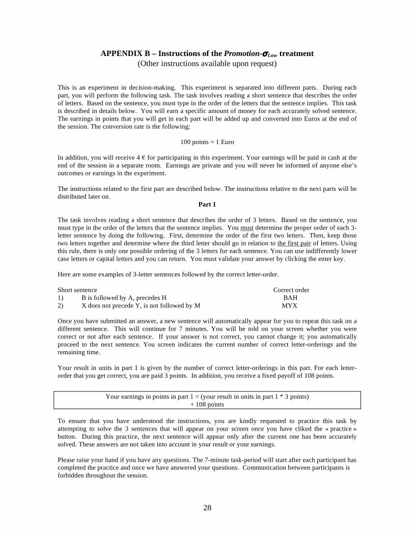
Part 1 The task involves reading a short sentence that describes the order of 3 letters. Based on the sentence, you must type in the order of the letters that the sentence implies. You must determine the proper order of each 3-letter sentence by doing the following. First, determine the order of the first two letters. Then, keep those two letters together and determine where the third letter should go in relation to the first pair of letters. Using this rule, there is only one possible ordering of the 3 letters for each sentence. You can use indifferently lower case letters or capital letters and you can return. You must validate your answer by clicking the enter key. Here are some examples of 3-letter sentences followed by the correct letter-order. Short sentence Correct order 1) B is followed by A, precedes H BAH 2) X does not precede Y, is not followed by M MYX Once you have submitted an answer, a new sentence will automatically appear for you to repeat this task on a different sentence. This will continue for 7 minutes. You will be told on your screen whether you were correct or not after each sentence. If your answer is not correct, you cannot change it; you automatically proceed to the next sentence. You screen indicates the current number of correct letter-orderings and the remaining time. Your result in units in part 1 is given by the number of correct letter-orderings in this part. For each letter-order that you get correct, you are paid 3 points. In addition, you receive a fixed payoff of 108 points.

Your earnings in points in part 1 = (your result in units in part 1 * 3 points) + 108 points

To ensure that you have understood the instructions, you are kindly requested to practice this task by attempting to solve the 3 sentences that will appear on your screen once you have cliked the « practice » button. During this practice, the next sentence will appear only after the current one has been accurately solved. These answers are not taken into account in your result or your earnings. Please raise your hand if you have any questions. The 7-minute task-period will start after each participant has completed the practice and once we have answered your questions. Communication between participants is forbidden throughout the session.

29

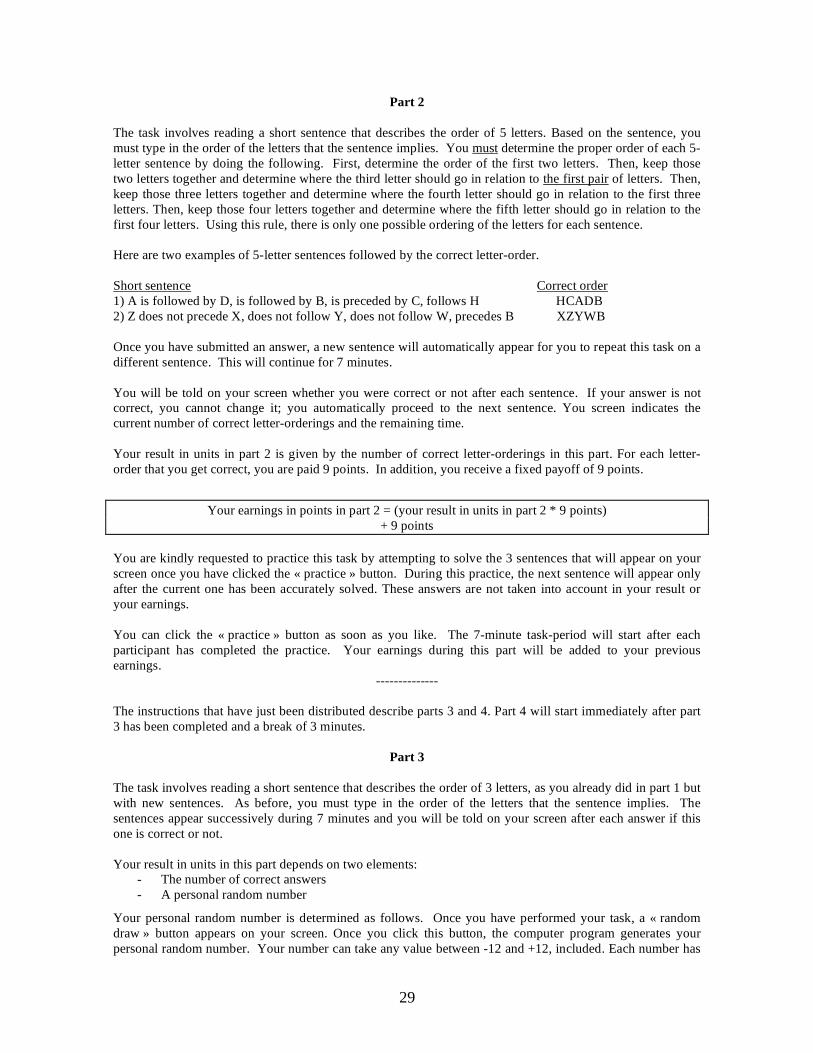
Part 2

The task involves reading a short sentence that describes the order of 5 letters. Based on the sentence, you must type in the order of the letters that the sentence implies. You must determine the proper order of each 5-letter sentence by doing the following. First, determine the order of the first two letters. Then, keep those two letters together and determine where the third letter should go in relation to the first pair of letters. Then, keep those three letters together and determine where the fourth letter should go in relation to the first three letters. Then, keep those four letters together and determine where the fifth letter should go in relation to the first four letters. Using this rule, there is only one possible ordering of the letters for each sentence. Here are two examples of 5-letter sentences followed by the correct letter-order. Short sentence Correct order 1) A is followed by D, is followed by B, is preceded by C, follows H HCADB 2) Z does not precede X, does not follow Y, does not follow W, precedes B XZYWB Once you have submitted an answer, a new sentence will automatically appear for you to repeat this task on a different sentence. This will continue for 7 minutes. You will be told on your screen whether you were correct or not after each sentence. If your answer is not correct, you cannot change it; you automatically proceed to the next sentence. You screen indicates the current number of correct letter-orderings and the remaining time. Your result in units in part 2 is given by the number of correct letter-orderings in this part. For each letter-order that you get correct, you are paid 9 points. In addition, you receive a fixed payoff of 9 points.

Your earnings in points in part 2 = (your result in units in part 2 * 9 points) + 9 points

You are kindly requested to practice this task by attempting to solve the 3 sentences that will appear on your screen once you have clicked the « practice » button. During this practice, the next sentence will appear only after the current one has been accurately solved. These answers are not taken into account in your result or your earnings. You can click the « practice » button as soon as you like. The 7-minute task-period will start after each participant has completed the practice. Your earnings during this part will be added to your previous earnings.

-------------- The instructions that have just been distributed describe parts 3 and 4. Part 4 will start immediately after part 3 has been completed and a break of 3 minutes.

Part 3 The task involves reading a short sentence that describes the order of 3 letters, as you already did in part 1 but with new sentences. As before, you must type in the order of the letters that the sentence implies. The sentences appear successively during 7 minutes and you will be told on your screen after each answer if this one is correct or not. Your result in units in this part depends on two elements:

- The number of correct answers - A personal random number

Your personal random number is determined as follows. Once you have performed your task, a « random draw » button appears on your screen. Once you click this button, the computer program generates your personal random number. Your number can take any value between -12 and +12, included. Each number has

30

an equally likely chance to be drawn. There is an independent random draw for each participant. Your personal random number is independent of your performance at the task.

Your result in units in part 3 is given by the addition of the number of correct answers and your personal random number in this part.

Your result in units in part 3 = your number of correct answers in part 3 + your personal random number in part 3

For example, if you give 38 correct answers and you draw a random number of -3, then your result is 35 units (i.e. 38-3). If, in contrast, you give 27 correct answers and you draw a random number of +3, then your result is 30 units (i.e. 27+3). Once you have drawn your number, you are informed on your result in units and on your earnings in points in part 3. For each unit, you get paid 3 points. In addition, you receive a fixed payoff of 108 points.

Your earnings in points in part 3 = (your result in units in part 3 * 3 points) + 108 points

It is important to note that this is your result in this part (your number of correct answers + your random number) that will determine the type of task you will perform in part 4.

Part 4

At the beginning of part 4, you are informed on your assignment to 3-letter sentences or to 5-letter sentences during this new part. Your assignment depends on your result in units during part 3.

- If your result in units in part 3 (i.e. your number of correct answers + your random number) amounts to 68 or more, then you are assigned to solving 5-letter sentences under the conditions detailed below.

- If your result in units in part 3 is lower than 68 units, then you are assigned to solving 3-letter sentences under the conditions detailed below.

Whatever your assignment is, you will solve sentences during 7 minutes. Your result in units in part 4 is given by the addition of the number of correct answers and your personal random number in this part.

Your result in units in part 4 = your number of correct answers in part 4 + your personal random number in part 4

Here are described the rules for each type of assignment.

◊ If your result in part 3 assigns you to 3-letter sentences

Once you have performed your task, you click the « random draw » button that generates your personal random number. Your number can take any value between -12 and +12, included. Each number has an equally likely chance to be drawn. There is an independent random draw for each participant.

You are then informed on your result in units and on your earnings in points in this part. For each unit, you get paid 3 points. In addition, you receive a fixed payoff of 108 points.

Your earnings in points in part 4 if assigned to 3-letter sentences = (your result in units in part 4 * 3 points) + 108 points

31

◊ If your result in part 3 assigns you to 5-letter sentences

Once you have performed your task, you click the « random draw » button that generates your personal random number. Your number can take any value between -4 and +4, included. Each number has an equally likely chance to be drawn. There is an independent random draw for each participant.

You are then informed on your result in units and on your earnings in points in this part. For each unit, you get paid 9 points. In addition, you receive a fixed payoff of 9 points.

Your earnings in points in part 4 if assigned to 5-letter sentences = (your result in units in part 4 * 9 points) + 9 points

Although your assignment to one task or the other depends exclusively on your result in part 3, you will be asked to indicate which task you would prefer being assigned to in part 4 is you would have the choice : Either the 3-letter sentences, with a random number between -12 et +12, a payoff of 3 points per unit and a fixed payoff of 108 points Or the 5-letter sentences, with a random number between -4 et +4, a payoff of 9 points per unit and a fixed payoff of 9 points. You will be requested to submit your answer at the beginning of part 4. Your earnings during these two parts will be added up to your previous payoffs. Please raise your hand if you have any questions regarding these instructions. We remind you that communication between participants is still forbidden.

____________