Embed Size (px)
Citation preview

The Personal-Tax Advantages of Equity�
Richard C. Greenand
Burton Hollifield
Graduate School of Industrial AdministrationCarnegie Mellon University
December 23, 1999
�Discussions with Pierre Collin–Dufresne, Bob Dammon, John Graham, Nathalie Moyen, Jim Poterba, and Bryan
Routledge have been very helpful to us. We would also like to thank seminar participants at GSIA, Rochester andTexas A & M for helpful comments.

Abstract
We compute the value of a firm that pays its cash flows each period through share repurchases in a dynamicenvironment where personal taxes are paid on realized capital gains and dividends. These results provide ameasure of the personal tax advantages of equity financing relative to debt financing, which are often citedas increasing the cost of debt. The initial price of the firm depends on the present value of the taxes paid,which, in turn, depends on the initial price. We solve this valuation problem in closed form in a deterministicsetting and numerically in a stochastic setting. We find significant valuation effects from the tax protectionafforded by the equity basis. The tax savings are on the order of 40-50% of the taxes paid by the shareholdersof firm that distributes cash through dividends, and the cost of capital is reduced by approximately .8 to 1.2percentage points through the use of repurchases relative to dividends.

1 Introduction
The Modigliani and Miller (1963) model of capital structure choice under taxation still forms the theoreti-
cal basis for most pedagogy and practice in modern Finance, despite its obvious empirical and theoretical
limitations. This theory predicts a corner solution of all debt financing for all firms, due to the deductibility
of interest payments at the corporate level. Such an outcome, however, appears grossly at variance with
observed practices and has never been taken seriously as a policy recommendation.
To explain this discrepancy, textbooks have followed researchers in pointing to three considerations that
are ignored in the Modigliani and Miller (hereafter, M&M) valuation of the tax shields from debt:
1. Costs of financial distress
2. Redundancy of corporate tax shields
3. Tax advantages to equity at the level of personal taxes.
While considerable research has been devoted to all three of these lines of inquiry, and this research has en-
riched considerably our qualitative understanding of the tradeoffs involved, it has proved difficult to generate
the sort quantitative results that could help researchers evaluate the empirical evidence or help practitioners
determine how much debt is too much debt.
With regard to the costs of distress, the M&M model takes as fixed and exogenous the firm’s operating
policies, assets, and net cash flows. It thus ignores the bankruptcy costs and incentive problems that may
distort real choices when the firm is in, or close to, bankruptcy. A great deal of research in the last two
decades has been devoted to this issue, and much has been learned about the ways incentive and informa-
tion problems can influence capital structure. Examples of this work include Jensen and Meckling (1976),
Myers (1977), Leland (1998), Parrino and Weisbach (1999) and Moyen (1999). The stylized nature of the
models used to capture these tradeoffs, however, makes their quantitative importance difficult to assess. Are
these costs sufficiently large to explain the low levels of debt finance firms employ? Or, are they relatively
insignificant when compared to the tax benefits of debt, as suggested by the analogy in Miller (1977) to the
recipe for “horse and rabbit stew?”
Second, the M&M model surely overstates the tax benefits of debt at the corporate level. The tax
shields from interest may, in some states of the world, be redundant, which lowers their expected value.
1

They may also be risky, which lowers their present value. Models that qualitatively describe the tradeoffs
this would impose upon the firm go back to DeAngelo and Masulis (1980), but the dynamic nature of
the treatment of tax shields in the tax code has made it difficult to evaluate the quantitative importance of
these considerations. Considerable progress has been made on this front recently, using methods based on
simulation, in Graham (1996), and especially Graham (1998).
In this paper, we focus on the third factor that investigators have cited in arguing that M&M overstate
the tax benefits of debt financing. Debt is tax-disadvantaged at the personal level. Interest payments are
taxed as ordinary income. Much of the compensation received by equity holders, on the other hand, comes
in the form of capital gains. Miller (1977) argued that this may raise the risk-adjusted cost of debt to the
firm, relative to equity, sufficiently to neutralize the tax advantages of debt at the corporate level.
The personal tax advantages of equity are largely attributable to the option to defer capital gains. The
value of this option, and thus the cost of equity capital to the firm, depends on the timing of the firm’s
cash distributions and the way those distributions are split between dividends and share repurchases. In
the interest of obtaining tractable expressions, however, researchers who have studied this problem in the
past have approached it with static models, making it very difficult to evaluate the quantitative realism or
importance of the effects they describe. Miller (1977), for example, simply assumes payments to equity are
tax exempt. This is clearly not the case. Even if all cash is distributed through repurchases, investors may
have to realize capital gains in order for the distribution to take place. DeAngelo and Masulis (1980) assume
a constant, exogenous personal tax rate on equity. Graham (1998) assumes the personal tax rate on equity is
a simple linear function of the dividend payout.
Our purpose here is to provide more quantitative guidance as to the magnitude and determinants of the
personal tax advantages of equity financing to the firm in a dynamic model. The model follows the original
M&M approach of taking as exogenous the firm’s pre-tax net operating cash flows. Thus, we abstract from
bankruptcy costs and incentive problems. We also ignore the complications at the corporate level studied by
Graham (1998). Our model is also partial equilibrium in the sense of taking as exogenous the pricing kernel.
Despite these obvious simplifications, this model allows us to pose and answer the following questions: In
an environment where the firm can issue debt or equity, and where it can distribute cash through repurchases
or dividends, how high is the risk-adjusted cost of equity relative to the risk-adjusted cost of debt? How
does this depend on the mix between debt and equity? How does it depend on the firm’s dividend policy?
2

We address these questions, first, in a setting that assumes certain and perpetual cash flows. This allows
for closed-form expressions for the firm’s value, cost of capital, and the gains to leverage. These expressions
can be directly compared to the traditional analyses in M&M, and Miller (1977). The certainty case also
illustrates the logic we employ in our numerical analysis of the firm’s problem under uncertainty.
Next we describe methods for obtaining numerical solutions to the model when the firm’s net cash flows
are random, but positive. Using these methods we calculate the value of the firm when all cash flows are
distributed through repurchases. Comparisons of this value to the value under full dividend payout provides
measures of the effects of the personal tax advantages of equity on the firm’s cost of funds.
When net cash flows can be negative, the state space for the valuation problem expands quickly, making
it difficult to solve the model numerically. New shares issued to finance negative net cash flows establish
new basis values, and the number of shares outstanding at all basis values must be tracked. To evaluate the
importance of these effects, we provide approximations by simulating the personal taxes paid assuming the
firm’s aggregate value evolves exogenously. We then compute the expected present value the taxes paid, and
numerically adjust the tax rate in the exogenous value process so that the basis values at which new shares
are issued approximately reflects the present value of future personal tax liabilities. For the cases where we
have full solutions to the model, this method provides reasonably accurate approximations. We then use
this method to evaluate the magnitude of the tax advantages provided by issuing new shares, at higher basis
values, as the firm moves through time.
Our results show that the personal-tax advantage of repurchases over dividends or interest payments
is substantial. The present value of tax savings are in the range of 40-50 percent of the present value of
the personal tax liability that would be incurred using only dividend payouts. The “implicit tax rates” we
calculate, rates which yield the same present value for the firm if all distributions were fully taxed, are
generally around 60 percent of the tax rate faced by the the firm’s shareholders.
To focus directly on the personal-tax consequences of the firm’s cash distribution policies, we abstract
from a number of considerations that have been important in other research on capital gains taxation.
We ignore liquidity needs or portfolio rebalancing that may lead individual investors to realize gains
even if it is disadvantageous from a tax standpoint to do so. The only motive in our model for realizing
gains is to facilitate the firm’s need to disgorge cash, and the firm repurchases shares at a price that fully
compensates the selling shareholder for surrendering the opportunity to continue deferring. In contrast, a
3

large literature in public economics studies the effects taxation based on realization rather than an accrual
has on the “effective tax rate” faced by individual investors. (See Poterba (1999) for a recent summary of
these results in the context of the measurement of after-tax returns for investors.) For example, Bailey (1969)
finds that the option to defer gains reduces their effective taxation by roughly a half, and the opportunity to
step up the basis on death reduces it by another half, leading to effective taxation at a rate one-fourth of the
statutory rate. This approximation has, in turn, been carried through by many authors, though Balcer and
Judd (1987) criticizes this approach. In their dynamic model no constant, proportional, “implicit” rate exists
that gives rise to the same investment and consumption behavior as capital gains taxation on a realization
basis.
Our results, since they ignore any other motives for realization, can be viewed as estimating the effect of
the firm’s need to distribute cash on the implicit rate at which capital gains are taxed. To the extent that other
motives exist, our results will understate the total tax burden born by equity holders, and hence the advantage
of equity repurchases relative to dividends or debt. Similarly, in order to focus purely on the effects of the
firm’s distribution policies, we assume the rates at which dividends, interest, and capital gains are taxed are
identical, and abstract from the distinction between long- and short-term gains. These assumptions will lead
us to undervalue the personal-tax benefits of equity financing. We also take the net cash flows of the firm as
exogenous. This abstracts from the firm’s ability to retain funds to delay taxation at the personal level.
The paper is organized as follows. The next section we evaluate the value the firm and determine its
cost of funds under certainty. In Section 3 we provide numerical solutions to the valuation problem under
uncertainty. In Section 4 we develop an approximation to the value when there are negative cash flows by
simulating the personal tax liability when the dynamics of the firm’s value are taken as exogenous. Section 5
provides a brief summary of our conclusions. All proofs are contained in the appendix.
2 The Certainty Case
Before studying environments where closed-form solutions are inaccessible, it is helpful to first understand
the simplest cases and examples. We begin, therefore, by evaluating the dynamics of the stock price, number
of shares outstanding, firm value, and cost of capital under a certainty model for the firm’s net cash flows.
We assume these cash flows are constant and perpetual, as in M&M, or that the cash flows grow at a constant
rate. We will provide solutions for each of the following cases, in order of complexity.
4

1. Full, or zero, taxation of all distributions. This covers the cases of full dividend payout, no taxation at
the personal level, and taxation of all capital gains whether realized or deferred.
2. Personal taxes paid only when gains are realized.
3. Debt is tax deductible at the corporate level, while personal taxes are paid on capital gains only on
realization.
4. Cash flows grow at a constant rate, while personal taxes paid only when gains are realized.
Throughout, we assume that interest, dividends, and realized capital gains are taxed at the same rate at
the personal level. For cases 1 and 2, we assume the firm is entirely equity financed. The firm’s cost of
capital, then, is the cost of equity. The cash flows the firm pays out should be viewed as net cash flow, after
corporate taxes. When we consider the third case, we treat corporate taxes explicitly.
The firm can be viewed as simply a sequence of certain, perpetual cash flows, Ct , paid at periodic
intervals, indexed by t � 0 ��������� ∞. This cash flow, and the investment and operating activities that produce
it, are viewed as exogenous. Thus, we consider only the financial activities of the firm, and ignore the
possibility that it may wish to retain funds to shield or defer taxation at the personal level. Again, these
simplifying assumptions are in keeping with the benchmark case provided by M&M.
Let the value of the firm at time t be Vt , the price per share be pt , and the number of shares outstanding
nt . When the firm is initially established, n0 shares are issued. The firm’s cash flows will be paid out either
as dividends or through repurchases of the shares initially issued. After this date, as the firm’s net cash flows
are always positive, no new shares are issued.
We ignore consumption or portfolio rebalancing as motives for trade. We also abstract from the distinc-
tion between long-term and short-term capital gains. Further, all investors face the same constant after-tax
discount rate, r � 0. Thus, investors can be viewed as homogeneous, and will not trade privately in equilib-
rium as long as the price sequence is increasing through time. It will never benefit an individual shareholder
realize a capital gain, pay taxes in the current period, and then reset the basis to shield income in the future.
Deferring the gain instead provides a tax-free loan from the government. By similar reasoning, a buyer will
not be willing to pay what a seller would demand for her shares, unless the buyer was motivated by some
other consideration such as desire for consumption or portfolio rebalancing. Since taxes incurred through
a transaction will be reflected in the price at which the transaction is executed, if the taxes represent a net
5

loss to the traders, one of them must find the trade unattractive at any price the other finds acceptable. The
next lemma establishes this result formally. It will be the basis for our arguments later that we can focus
exclusively on the trades between the firm and its initial shareholders. The proof, which is provided in the
Appendix, simply relies on the argument that for any feasible realization strategy, the benefits associated
with future tax deductions from the step up of the basis will have a lower present value than the taxes that
must be paid now to achieve that increase in the basis.
Lemma 1 Suppose the current price exceeds the initial price at which the shares were issued, pt�
po, and
that all current equity claimants hold the shares with a tax basis of po. Then a new shareholder would
be willing to buy shares at pt only if that price is less than or equal to the minimum price an existing
shareholder would accept for her shares.
2.1 Benchmark Cases
The next proposition provides formulas for the firm’s value and share price dynamics, when there are no
taxes or when taxation is symmetric for capital gains and dividends. In keeping with the M&M model, we
view the cash flows as constant: Ct � C. The algebra leading to these formulas, is detailed in the Appendix.
Let pct denote the cum-dividend price, and let pe
t be the ex-dividend price.
Proposition 1 When capital gains are taxed each period, whether realized or deferred, and dividends are
taxed as ordinary income, the price per share and number of shares obey the following dynamics:
1. When cash flows are paid as dividends, the number of shares, cum-dividend price, and ex-dividend
price are constant through time.
pct � 1
n0
C 1 � τp �� C 1 � τp �
r � � (1)
pet � 1
n0
C 1 � τp �r
� (2)
and nt � n0.
6

2. When cash flows are used for repurchases, the price per share grows geometrically and the number
of shares shrinks geometrically, at the pre-tax rate of interest, r �� 1 � τ p � .pt � 1 � pt
1 r
1 � τp � � (3)
nt � 1 � nt
1 r1 � τp
� (4)
3. In both cases the aggregate, ex-distribution value, denoted Vt , is constant though time,
Vt � Cr
1 � τp
� (5)
These formulas include the special case of no taxation when τp � 0, in which case the number of shares
shrinks, and the price grows, at rate r.
The proposition shows that, when capital gains are taxed whether realized or deferred, the decision to
distribute cash by dividend or capital gain has no effect on aggregate firm value or aggregate personal tax
liability. The shares actually repurchased in the distribution are only partially taxed, due to protection from
the basis. In the M&M setting, however, the aggregate capital gain on all outstanding shares is precisely
equal to the amount of the distribution, and hence the aggregate tax liability is the same as it would be under
full dividend payout.
2.2 Repurchases when Taxes are Paid On Realized Gains Only
When capital gains are not taxed when earned, but rather when realized, there is a wedge between the value
of a share to a purchaser, who establishes a new basis at the current price, and the value to a shareholder who
holds the share at a lower basis. In our model, there is no motive to trade other than to distribute cash from
the firm. Lemma 1 implies that if the price is increasing, the price demanded by an existing shareholder,
with an embedded gain, exceeds the price a new, private buyer would be willing to pay. Thus, the firm issues
shares only at its founding, and all shareholders hold the shares with the same basis, po. We will assume
that the price the firm pays for the shares it repurchases fully compensates the shareholder for the loss of
the opportunity to defer. Then Lemma 1 implies that this price does, in fact, exceed what a private buyer
7

would be willing to pay. Note that the one point where a new buyer and a seller would view the shares
symmetrically is at the initial date, since selling the shares at po triggers no tax liability.
We normalize the number of shares originally issued to n0 � 1. At any point we know that
Ct �� nt � 1 � nt � pt � (6)
since the value of the shares repurchased must equal the cash used to repurchase them. Thus, nt is the
number of shares prevailing between the distribution at time t and the distribution at t 1.
If an investor sells a share at time t, she would realize a cash flow of
pt 1 � τp �� τp po
and if she holds and sells next period, she realizes a cash flow of
pt � 1 1 � τp �� τp po �Equating the present values of these two alternatives gives us a difference equation for the price.
pt 1 � τp �� τp po � 1
1 r � � 1 � τp � pt � 1 τp po � � (7)
Given a price series satisfying this equation at each point in time, a shareholder is, by recursive argument,
indifferent between selling shares back to the firm immediately or deferring the gain to an arbitrary point in
the future.
The indifference condition, (7), can be rearranged to give
pt � 1
1 r � pt � 1 � r
τp
1 � τppo � � (8)
Solving (8) yields the share price
pt � θ 1 r � t � τp
1 � τppo �
where θ and the initial value of the equity, po, are coefficients to be determined. Evaluating the stock price
8

at time 0, and solving for θ,
θ � po
1 � τp�
and so
pt � po
1 � τp � 1 r � t � τp � � (9)
We can now establish the initial value of the firm, po. Since buyers and sellers will view the shares
symmetrically at this point, this price must simply be the present value of the aggregate after-tax cash flows
to the equity holders. The after-tax cash flows accruing to initial equity holders at time t are the after-tax
proceeds from the shares repurchased at that time,
nt � 1 � nt � pt 1 � τp �� τp po � � Ct 1 � τp �� nt � 1 � nt � τp po� Ct 1 � τp �� nt � 1 � nt � τp ptpo
pt� Ct 1 � τp �� Ctτppo
pt� Ct 1 � τp � 1 τp 1 r � t � τp �� Ct 1 � τp � 1 r � t 1 r � t � τp� (10)
The first line uses the constraint that the value of the shares repurchased must equal the cash distributed,
equation (6). The third line uses this constraint again, and the fourth line uses the solution for the price, (9).
The limit, as t � ∞, of the right-hand side of (10) is Ct 1 � τp � . As time passes, the aggregate value
of the protection afforded by the initial basis becomes trivially small. The share price rises at close to a
geometric rate as shares are extinguished through repurchases. In the limit, therefore, the distribution is
fully taxed.
The derivation to this point allows for any deterministic pattern of positive cash flows over time. When
these flows are constant, it is simple to compute the initial share price, po, as the present value of after–tax
flows
po � ∞
∑s � 1
1 1 r � sC 1 � τp � 1 r � s 1 r � s � τp� C 1 � τp � ∞
∑s � 1
1 1 r � s � τp� (11)
9
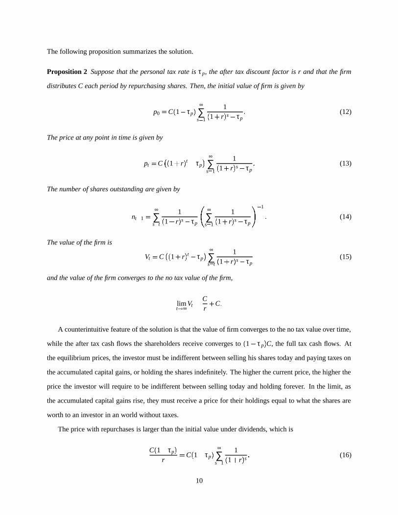
The following proposition summarizes the solution.
Proposition 2 Suppose that the personal tax rate is τp, the after tax discount factor is r and that the firm
distributes C each period by repurchasing shares. Then, the initial value of firm is given by
p0 � C 1 � τp � ∞
∑s � 1
1 1 r � s � τp� (12)
The price at any point in time is given by
pt � C � 1 r � t � τp � ∞
∑s � 1
1 1 r � s � τp� (13)
The number of shares outstanding are given by
nt � 1 � ∞
∑s � t
1 1 r � s � τp � ∞
∑s � 1
1 1 r � s � τp � � 1 � (14)
The value of the firm is
Vt � C � 1 r � t � τp � ∞
∑s � t
1 1 r � s � τp(15)
and the value of the firm converges to the no tax value of the firm,
limt � ∞
Vt � Cr C �
A counterintuitive feature of the solution is that the value of firm converges to the no tax value over time,
while the after tax cash flows the shareholders receive converges to 1 � τ p � C, the full tax cash flows. At
the equilibrium prices, the investor must be indifferent between selling his shares today and paying taxes on
the accumulated capital gains, or holding the shares indefinitely. The higher the current price, the higher the
price the investor will require to be indifferent between selling today and holding forever. In the limit, as
the accumulated capital gains rise, they must receive a price for their holdings equal to what the shares are
worth to an investor in an world without taxes.
The price with repurchases is larger than the initial value under dividends, which is
C 1 � τp �r
� C 1 � τp � ∞
∑s � 1
1 1 r � s � (16)
10

The personal-tax advantage of equity, in this setting, is manifest in the fact that the personal tax rate is
subtracted in the “discount factors” in equation (12), but not in (16).
By truncating the infinite sum in (12), these expressions can be compared quantitatively. Figure 1 plots
the present value of taxes paid under repurchases, which is C � r � � po as a fraction of the present value of
taxes paid under dividends, τpC � r, for a firm with cash flow of 100. The value of the firm, po is computed
with 500 terms in the summation. The figure plots these ratios against the personal tax rate, using three
different values for the after-tax discount rate, 3% (+), 6% (*), and 9% (x). In each case, repurchases save
the firm’s shareholders 40-50% in the present value of their tax liability.
The firm’s cost of equity capital is simply the discount rate that equates the initial value given above to
the present value of the pre-personal-tax cash flows. That is, the cost of equity, r, solves
po � Cr� (17)
Figure 2 plots this cost of equity capital, assuming pre-tax return of 6%, for various levels of the tax rate
from 0 to 40%. The solid line is the cost of equity capital, in this case where C � 1 just 1po
. The dotted line
is the cost of capital prevailing when distributions are paid as dividends, r �� 1 � τ p � .2.3 Allowing for Growth
Our formulas for the initial value of the firm generalize in a straightforward manner to the case of constant
growth in the cash flows. Up to equation (10), the derivation applies to any positive, deterministic series of
net cash flows. If these cash flows grow at a constant rate, g, with an initial cash flow at date t=1 of C, we
have, as in equation (11),
po � C 1 � τp � ∞
∑s � 1
1 g � s � 1 1 r � s � τp� (18)
Table 1 provides measures of the tax advantage to repurchases versus dividends under different growth
rates. In the table, the implict tax rate is the rate that equates the present value of the fully taxed cash flows
to the initial value of the firm: τ � solving po � C 1 � τ � � �� r � g � . The percent of PV taxes is computed
by calculating the present value of taxes paid as a percentage of the present value of taxes paid under
full, proportional taxation. The table shows quite clearly that the advantages of repurchases over dividend
payments decrease with the rate of growth in the cash flows, despite the fact that the growth in the firm’s
11
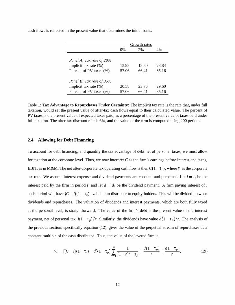
cash flows is reflected in the present value that determines the initial basis.
Growth rates0% 2% 4%
Panel A: Tax rate of 28%Implicit tax rate (%) 15.98 18.60 23.84Percent of PV taxes (%) 57.06 66.41 85.16
Panel B: Tax rate of 35%Implicit tax rate (%) 20.58 23.75 29.60Percent of PV taxes (%) 57.06 66.41 85.16
Table 1: Tax Advantage to Repurchases Under Certainty: The implicit tax rate is the rate that, under fulltaxation, would set the present value of after-tax cash flows equal to their calculated value. The percent ofPV taxes is the present value of expected taxes paid, as a percentage of the present value of taxes paid underfull taxation. The after-tax discount rate is 6%, and the value of the firm is computed using 200 periods.
2.4 Allowing for Debt Financing
To account for debt financing, and quantify the tax advantage of debt net of personal taxes, we must allow
for taxation at the corporate level. Thus, we now interpret C as the firm’s earnings before interest and taxes,
EBIT, as in M&M. The net after-corporate tax operating cash flow is then C 1 � τc � , where τc is the corporate
tax rate. We assume interest expense and dividend payments are constant and perpetual. Let i � it be the
interest paid by the firm in period t, and let d � dt be the dividend payment. A firm paying interest of i
each period will have C � i � 1 � τc � available to distribute to equity holders. This will be divided between
dividends and repurchases. The valuation of dividends and interest payments, which are both fully taxed
at the personal level, is straightforward. The value of the firm’s debt is the present value of the interest
payment, net of personal tax, i 1 � τp � � r. Similarly, the dividends have value d 1 � τp � � r. The analysis of
the previous section, specifically equation (12), gives the value of the perpetual stream of repurchases as a
constant multiple of the cash distributed. Thus, the value of the levered firm is:
VL ���� C � i � 1 � τc � � d ! 1 � τp � ∞
∑s � 1
1 1 r � s � τp d 1 � τp �
r i 1 � τp �r
� (19)
12

This can be written as the value of an unlevered firm, with all cash distributed through repurchases, as in
equation (12), plus the net advantages/disadvantages of dividends and debt,
VL � C 1 � τc � 1 � τp � ∞
∑s � 1
1 1 r � s � τp d 1 � τp � � 1
r� ∞
∑s � 1
1 1 r � s � τp � i 1 � τp � � 1r�" 1 � τc � ∞
∑s � 1
1 1 r � s � τp � � (20)
This equation is linear in both i and d, so that dividend policy and capital structure policy will be charac-
terized by corner solutions in this environment. Dividends are dominated. The term multiplying d 1 � τ p �in equation (20) is unambiguously negative for any τp � 0. The relative attractiveness of debt versus equity
(with repurchases) is determined by the relative magnitudes of r, τ p, and τc. Assuming d � 0, we can rewrite
the contribution of debt to the value of the firm as
i 1 � τp �r � 1 � r 1 � τc � ∞
∑s � 1
1 1 r � s � τp � � DL � 1 � r 1 � τc � ∞
∑s � 1
1 1 r � s � τp � � (21)
where DL is the value of the debt. The term multiplying DL is the gain to leverage, and can be instructively
compared to the gain to leverage in Miller (1977), which treats the equity flows as fully taxed, but at a
preferential rate, τs,
1 � 1 � τc � 1 � τs �1 � τp
�In our setting the flows to equity are not taxed at a preferential rate. Rather the personal-tax advantage to
equity comes from the present value of the tax shields from the initial basis.
While providing a quantitative benchmark for the personal tax advantages of equity, this analysis will
not, of itself, rationalize interior capital structures at realistic values of the parameters. Our intent is, rather,
to gain a better understanding of how large other costs of debt, such as losses in aggregate value associated
with financial distress, would have to be to generate interior optima. We can rewrite the gain to leverage,
per dollar of debt issued, as follows:
r � 1r�# 1 � τc � ∞
∑s � 1
1 1 r � s � τp � � r � ∞
∑s � 1
1 1 r � s � 1 � τc � 1 r � s � τp �� r � ∞
∑s � 1
1 r � sτc � τp 1 r � s �� 1 r � s � τp � � (22)
13

The denominator in each term in this summation is positive. Since 1 r � s � 1, the following lemma follows
by inspection of the numerator.
Lemma 2 When τp $ 1 r � τc the gain to leverage is positive.
Inspection of (22) suggests, indeed, that the personal tax rate must be substantially higher than the
corporate rate to offset the benefits of deductions at the corporate level. Figure 3 provides a quantitative
sense of this. The figure plots the corporate tax rate at which the gain to leverage is zero, for different values
of the personal tax rate. For a given personal tax rate, at corporate rates above the curve plotted in the figure,
the firm would prefer debt financing over equity financing.
Equation (19) for the value of the firm can also be used to evaluate the effects of capital structure and
dividend policy on the firm’s overall cost of capital. In a manner analogous to M&M, we ask what discount
rate sets the present value of future after-corporate-tax, operating cash flow equal to the value of the firm.
We solve for r in
VL � C 1 � τc �r
(23)
where VL is computed using (19). Table 2 reports the results of these computations for a firm with τc � 34%,
r � 6%, and two values of the personal tax rate, 28% and 35%.
3 Uncertain Cash Flows
When cash flows are certain, in a setting parallel to that envisioned by M&M, we can solve for the value of
the firm under repurchases in closed form. The advantage repurchases provide over dividends is attributable,
in our setting, entirely to the tax shield supplied by the initial basis. It takes a mathematically simple form
as a reduction in the discount factors attributable to after-tax cash flows (see equations (12) and (16)). We
found that this advantage to repurchases is quantitatively substantial for reasonable parameter values, 40-
50% of the value of the personal tax liability. It was not, however, sufficiently large to completely offset the
advantages at the corporate level of debt that, as assumed by M&M, offers full, non-redundant tax shields at
the corporate level.
Our purpose in this section is to evaluate whether these implications hold when cash flows are uncertain.
We continue to make assumptions analogous to M&M. We view the firm as a perpetual stream of pre-tax
14

Dividend Payout RatioInterest over EBIT 0% 20% 40% 60% 80% 100%Panel A: τp � 28%0% 7.14 7.35 7.57 7.81 8.06 8.3320% 6.74 6.89 7.04 7.21 7.38 7.5540% 6.38 6.48 6.58 6.69 6.80 6.9160% 6.06 6.12 6.18 6.24 6.30 6.3780% 5.77 5.79 5.82 5.85 5.87 5.90100% 5.50 5.50 5.50 5.50 5.50 5.50Panel B: τp � 35%0% 7.55 7.84 8.15 8.48 8.84 9.2320% 7.21 7.41 7.63 7.86 8.11 8.3740% 6.89 7.03 7.18 7.33 7.49 7.6560% 6.60 6.69 6.78 6.87 6.96 7.0580% 6.34 6.38 6.42 6.46 6.50 6.54100% 6.09 6.09 6.09 6.09 6.09 6.09
Table 2: Cost of Capital Calculations: The body of the table reports the percentage return that equatesthe value of the firm to present value of after-tax operating cash flows. Rows represent different capitalstructures, parameterized by the percentage of pre-tax income paid in interest. Columns represent differentdividend policies, parameterized by the percentage of after-tax cash flow paid in dividends. The corporatetax rate is assumed to be 34%, the personal rate is 28% or 35%, and the after-tax discount rate is 6%.
net cash flows that are constant in expectation. Thus, when cash flows are paid as dividends, or when all
capital gains and losses are taxed symmetrically, whether realized or not, the value of the firm, denoted VF ,
is given by
VF � C 1 � τp �r
where C is the expected cash flow under the risk-neutral measure. Let Cst denote cash flow in state s at date
t. For simplicity, we take the state space to be finite and discrete, and assume net cash flows are independent
and identically distributed through time. Denote the risk-neutral probability of cash flow C st as πs.
When net cash flows are always positive, we solve numerically for the value of the firm. With positive
net cash flows, as under certainty, shares are only issued once, and so the basis is the same for all outstanding
shares. If the price always rises through time, as shares are retired, then this basis will always be the initial
price. The only state variables on which prices will depend are the current cash flow, Ct , and the number of
shares outstanding, nt � 1. For the no-tax case, it is simple to verify analytically that the price always rises
15

when net cash flows are positive.1 While we have not found a proof for the general case, we can verify
numerically that along the worst sample paths, where the lowest (but still positive) cash flow is realized, the
price increases through time with the repurchases.
While the decision rules for the firm are mechanical in this model, the share price must be determined
endogenously. The price a shareholder will demand when the firm offers to repurchase shares will depend
on the shareholder’s basis, and on the present value of future taxes paid if she decides not to sell her shares
back to the firm, which in turn will depend on the future price path. Suppose at date t we enter the period
with nt � 1 shares outstanding. If we know the price next period will be set so that a shareholder with basis po
will be just indifferent between continuing to hold the shares and selling into the repurchase, then the price
the shareholder would demand in the current period, pt , must satisfy:
pt 1 � τp �� τp po � 11 r
Et � pt � 1 ! 1 � τp �� τp po � � (24)
In addition, all cash must be distributed through the repurchase
nt � 1 � nt � pt � Ct � (25)
Finally, as there is no distribution at the initial date, t � 0, the initial price must be set to satisfy
po � 11 r
E0 � p1 ! 1 � τp �� τp po � (26)
1Let nt % 1 be the number of shares outstanding upon entering period t. The price at date t will satisfy the equalities:
pt & 1nt % 1 ' Ct ( ∞
∑s ) 1
Et * Ct + s,1 ( r - s .0/ & 1
nt ' ∞
∑s ) 1
Et * Ct + s,1 ( r - s .0/21
Therefore,
pt + 1 3 pt & 1nt ' Ct + 1 ( ∞
∑s ) 1
Et + 1 * Ct + 1 + s,1 ( r - s . 3 ∞
∑s ) 1
Et * Ct + s,1 ( r - s .0/& 1
nt 4 Ct + 1 ( Cr 3 C
r 5& 1nt
Ct + 1 1
16
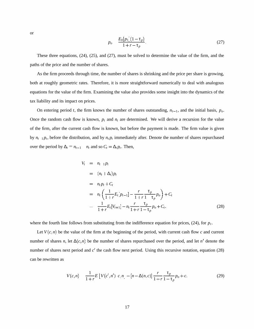
or
po � E0 � p1 ! 1 � τp �1 r � τp
� (27)
These three equations, (24), (25), and (27), must be solved to determine the value of the firm, and the
paths of the price and the number of shares.
As the firm proceeds through time, the number of shares is shrinking and the price per share is growing,
both at roughly geometric rates. Therefore, it is more straightforward numerically to deal with analogous
equations for the value of the firm. Examining the value also provides some insight into the dynamics of the
tax liability and its impact on prices.
On entering period t, the firm knows the number of shares outstanding, nt � 1, and the initial basis, po.
Once the random cash flow is known, pt and nt are determined. We will derive a recursion for the value
of the firm, after the current cash flow is known, but before the payment is made. The firm value is given
by nt � 1 pt , before the distribution, and by nt pt immediately after. Denote the number of shares repurchased
over the period by ∆t 6 nt � 1 � nt and so Ct � ∆t pt . Then,
Vt � nt � 1 pt� nt ∆t � pt� nt pt Ct� nt
1
1 rEt � pt � 1 7� r
1 rτp
1 � τppo � Ct� 1
1 rEt �Vt � 1 8� nt
r1 r
τp
1 � τppo Ct � (28)
where the fourth line follows from substituting from the indifference equation for prices, (24), for p t .
Let V c � n � be the value of the firm at the beginning of the period, with current cash flow c and current
number of shares n, let ∆ c � n � be the number of shares repurchased over the period, and let n 9 denote the
number of shares next period and c 9 the cash flow next period. Using this recursive notation, equation (28)
can be rewritten as
V c � n � � 11 r
E : V c 9 � n 9 �<;; c � n =>�#� n � ∆ n � c � r1 r
τp
1 � τppo c � (29)
17

The firm’s cash constraint can be rearranged to give
∆ c � n � � cp c � n � � cn
V c � n � � (30)
where the second equality follows since p c � n � � V c � n � � n. Substituting equation (30) into equation (29)
yields
V c � n � � 11 r
E : V c 9 � n 9 � ;; c � n =>� n � cn
V c � n � � r1 r
τp
1 � τppo c � (31)
Equation (31) is a functional equation that must be satisfied by V c � n � , and so the solution is a fixed–point
to equation (31). Assuming the firm begins with one share, and noting that there is no distribution between
t � 0 and t � 1, then
E0 � p1 ?� E :V c 9 � 1 �A@ n � 1 =� ∑s
πsV Cs � 1 � � (32)
Using this in the expression for po, (27), yields
po � E �V c 9B� 1 �A@ n � 1 < 1 � τp �1 r � τp
� (33)
Thus, we can solve for the value of the firm and the initial price by seeking a fixed point, V c � n � , to equations
(31) and equation (33).
To solve for this fixed point numerically, we pick a grid for the number of shares, C n � n1 � n2 ��������� 1 D ,and start with a guess for E �V c 9B� n 9 �0@ c � n for each of these points and for each cash flow outcome. We
set E �V c 9E� n 9 �0@ c � n equal to the no tax value for n F n, since as we show later, the value of the firm must
converge to the no–tax value as the number of shares goes to zero. We then guess the initial price, and
iterate as follows. Denote the guesses at the i’th iteration as ψi c � n � and pi0 respectively. Using these on the
right-hand side of equation (31), we solve for the firm value, which we denote V i c � n � . This step involves
solving a quadratic equation at each point c � n � . We can then use equation (30) to calculate the number of
shares repurchased at each point ∆i c � n � � cn � V i c � n � . Given these solutions, we compute new guesses for
18

the conditional expectations:
ψi � 1 c � n � � ∑s
πsV i �Cs � n � ∆i n � c � (34)
for each pair c � n � , and use equations (32) and (33) to compute a new guess of the initial price.
pi � 1o � ∑s πsV i Cs � 1 � 1 � τp �
1 r � τp(35)
These steps are repeated until we arrive at an approximate fixed point. In practice, this procedure converges
relatively quickly.
Table 3 provides numerical results obtained using this procedure for a firm with expected cash flows of
100. In each case there are two possible cash flows, and probability of the higher cash flow is 2 � 3. The
after-tax discount rate is 6%, and two values for τp are used, 28% and 35%.
The table provides various descriptive measures of the effects of personal taxation on the value. The
second column gives the tax rate that sets the present value of after-tax cash flows, assuming they were fully
taxed, equal to the actual value. That is, we solve
po � C 1 � τ � �r
(36)
for τ � . In every case, this implicit tax rate is substantially lower than the tax rate on dividends. The third row
measures the impact of the tax advantages to equity on the cost of funds to the firm. We find the discount
rate, r, that solves:Cr� po � (37)
The difference between this cost of capital and the pre-tax cost of capital under dividends is in every case
substantial, between 0.79 and 1.21 percentage points. The final row reports the present value of personal
taxes paid as a fraction of the present value of the tax liability under full dividend payout.
From this table we see that, as in the certainty case, the use of repurchases over dividends reduces the
present value of the shareholders’ personal tax liability by 40% to 50%. There is very little variation in
the quantities of interest across cash-flow outcomes of different volatility. This is not surprising, given the
nature of the tax liability. Through recursive substitution, and use of the budget constraint, we can rewrite
19

Cash Flow OutcomesFull tax C 120 � 60 D C 141 � 18 D No tax
Panel A: Tax rate of 28%Value 1,200.00 1,403.73 1,402.01 1,666.67Implicit tax rate (%) 28.00 15.78 15.88 0.00Cost of capital (%) 8.33 7.12 7.13 6.00Percent of PV taxes (%) 100.00 56.34 56.71 0.00
Panel B: Tax rate of 35%Value 1,083.33 1,327.71 1,325.45 1,666.67Implicit tax rate (%) 35.00 20.34 20.47 0.00Cost of capital (%) 8.33 7.53 7.54 6.00Percent of PV taxes (%) 100.00 58.11 58.49 0.00
Table 3: Numerical Measures of Tax Advantage to Equity: The implicit tax rate is the rate that, underfull taxation, would set the present value of after-tax cash flows equal to their calculated value. The costof capital is the discount rate that sets the present value of the pre-tax, expected cash flows equal to thecalculated value. The percent of PV taxes is the present value of expected taxes paid, as a percentage of thepresent value of taxes paid under full taxation. The tax rate is assumed to be 35%, the expected net cashflow before personal tax is 100, and the after-tax discount rate is 6%.
the equation for the firm’s value, (28), as:
Vt � Cr Ct �HGI nt � ∞
∑i � 1
Et J Ct K ipt K i L 1 r � i MN po
τp
1 � τp� (38)
Increases in volatility would affect the value through the effects of correlation between Ct � i and pt � i on
the expectation of their quotient, and through Jensen’s inequality. Since the price is growing geometrically,
however, these effects become relatively unimportant very quickly. The firm’s value is not sufficiently non-
linear in the cash flows for the volatility to have a significant effect, when the cash flows are uniformly
positive.
Equation (38) also makes clear that the value of the firm must, as time advances, approach the no tax
value. The number of shares is steadily decreasing, as cash is distributed through repurchases, so the middle
term involving the basis eventually becomes negligible. This implies that
limt � ∞
Vt � Cr Ct �
20
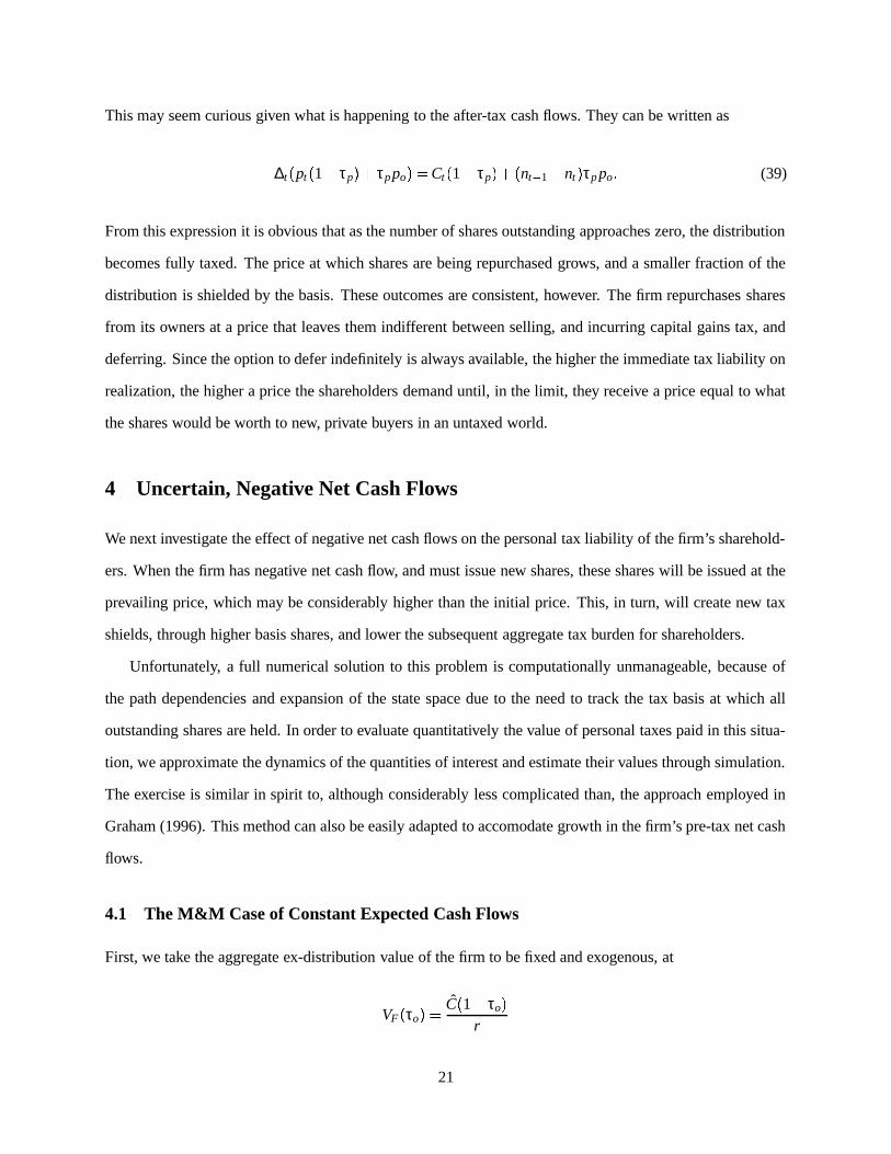
This may seem curious given what is happening to the after-tax cash flows. They can be written as
∆t pt 1 � τp �� τp po � � Ct 1 � τp �� nt � 1 � nt � τp po � (39)
From this expression it is obvious that as the number of shares outstanding approaches zero, the distribution
becomes fully taxed. The price at which shares are being repurchased grows, and a smaller fraction of the
distribution is shielded by the basis. These outcomes are consistent, however. The firm repurchases shares
from its owners at a price that leaves them indifferent between selling, and incurring capital gains tax, and
deferring. Since the option to defer indefinitely is always available, the higher the immediate tax liability on
realization, the higher a price the shareholders demand until, in the limit, they receive a price equal to what
the shares would be worth to new, private buyers in an untaxed world.
4 Uncertain, Negative Net Cash Flows
We next investigate the effect of negative net cash flows on the personal tax liability of the firm’s sharehold-
ers. When the firm has negative net cash flow, and must issue new shares, these shares will be issued at the
prevailing price, which may be considerably higher than the initial price. This, in turn, will create new tax
shields, through higher basis shares, and lower the subsequent aggregate tax burden for shareholders.
Unfortunately, a full numerical solution to this problem is computationally unmanageable, because of
the path dependencies and expansion of the state space due to the need to track the tax basis at which all
outstanding shares are held. In order to evaluate quantitatively the value of personal taxes paid in this situa-
tion, we approximate the dynamics of the quantities of interest and estimate their values through simulation.
The exercise is similar in spirit to, although considerably less complicated than, the approach employed in
Graham (1996). This method can also be easily adapted to accomodate growth in the firm’s pre-tax net cash
flows.
4.1 The M&M Case of Constant Expected Cash Flows
First, we take the aggregate ex-distribution value of the firm to be fixed and exogenous, at
VF τo � � C 1 � τo �r
21
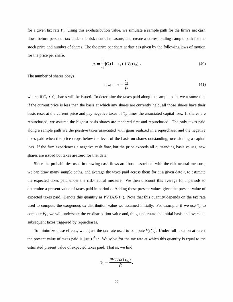
for a given tax rate τo. Using this ex-distribution value, we simulate a sample path for the firm’s net cash
flows before personal tax under the risk-neutral measure, and create a corresponding sample path for the
stock price and number of shares. The the price per share at date t is given by the following laws of motion
for the price per share,
pt � 1nt�Ct 1 � τo �� VF τo � O� (40)
The number of shares obeys
nt � 1 � nt � Ct
pt(41)
where, if Ct F 0, shares will be issued. To determine the taxes paid along the sample path, we assume that
if the current price is less than the basis at which any shares are currently held, all those shares have their
basis reset at the current price and pay negative taxes of τp times the associated capital loss. If shares are
repurchased, we assume the highest basis shares are tendered first and repurchased. The only taxes paid
along a sample path are the positive taxes associated with gains realized in a repurchase, and the negative
taxes paid when the price drops below the level of the basis on shares outstanding, occasioning a capital
loss. If the firm experiences a negative cash flow, but the price exceeds all outstanding basis values, new
shares are issued but taxes are zero for that date.
Since the probabilities used in drawing cash flows are those associated with the risk neutral measure,
we can draw many sample paths, and average the taxes paid across them for at a given date t, to estimate
the expected taxes paid under the risk-neutral measure. We then discount this average for t periods to
determine a present value of taxes paid in period t. Adding these present values gives the present value of
expected taxes paid. Denote this quantity as PVTAX τo � . Note that this quantity depends on the tax rate
used to compute the exogenous ex-distribution value we assumed initially. For example, if we use τ p to
compute VF , we will understate the ex-distribution value and, thus, understate the initial basis and overstate
subsequent taxes triggered by repurchases.
To minimize these effects, we adjust the tax rate used to compute VF τ � . Under full taxation at rate τ
the present value of taxes paid is just τC � r. We solve for the tax rate at which this quantity is equal to the
estimated present value of expected taxes paid. That is, we find
τ1 � PVTAX τo � rC
�22

We then repeat the simulation, calculate PVTAX τ1 � , and iterate in this way until we find that τk P τk � 1.
We find the tax rates converge very quickly. In effect, we are iteratively solving the equation
Cτ �r
� PVTAX τ � � � (42)
This approximation will give average taxes paid that are similar in magnitude to what we would expect
under a full solution for the equilibrium value of the firm. It will distort somewhat, however, the time path
of taxes paid. A check on the accuracy of the method can be made by implementing the approximation in
the certainty case, where we have an analytical solution for the equilibrium value, and in the case where
cash flows are all positive, where we have a numerical solution for the initial price. This exercise suggests
the approximation is quite accurate.
Table 4 provides results on the taxes paid under this approximation for the dynamics of firm value. We
assume there are two states for the pre-tax cash flow, which has an expected value of 100 in every period.
Thus, the model conforms to the M&M assumption of constant, perpetual expected cash flow. The after-tax
discount rate is assumed to be 6%. The table reports results for two tax rates and two levels of volatility
for the cash flows. It reports the same measures of the tax benefits of equity with repurchases as previously
reported for the cases of certainty and positive cash flows.
The difference between the cost of capital under repurchases and the pre-tax cost of capital under divi-
dends is in every case substantial. The implicit tax rate on equity flows is, again, substantially lower than the
personal tax rate, and the difference increases as the personal tax rate increases. The estimated present value
of personal taxes paid as a fraction of the present value of the tax liability under full dividend payout varies
between 55% and 65%. Over all, the magnitudes in Table 4 are similar to those reported for the certainty
case, and for the case where cash flows are strictly positive. The effective tax rate on flows to equity holders
is, for example, close to 20% when dividends are taxed at 35%. Thus, it appears that the tax shields afforded
by the original basis reduce the personal tax burden quite dramatically, but the equity is also far from tax
free as assumed in Miller (1977).
The present value of the tax liability appears to increase somewhat with the volatility of the cash flows.
This may seem surprising given that shareholders, who have freedom to defer or realize gains and losses,
have an option-like claim on their shares. The shape of the equity holders’ tax liability is ambiguous,
however. When the firm has a positive cash flow, the after-tax cash flow to equity is given by the right-hand
23
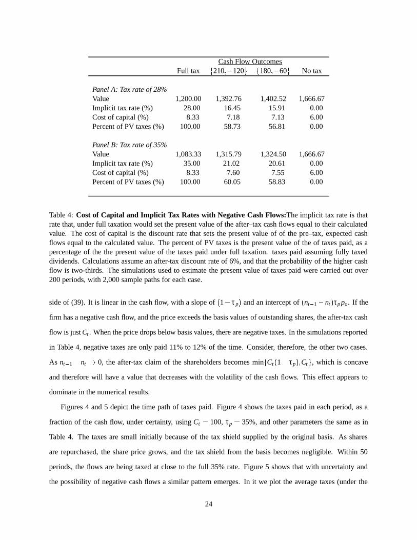
Cash Flow OutcomesFull tax C 210 ��� 120 D C 180 ��� 60 D No tax
Panel A: Tax rate of 28%Value 1,200.00 1,392.76 1,402.52 1,666.67Implicit tax rate (%) 28.00 16.45 15.91 0.00Cost of capital (%) 8.33 7.18 7.13 6.00Percent of PV taxes (%) 100.00 58.73 56.81 0.00
Panel B: Tax rate of 35%Value 1,083.33 1,315.79 1,324.50 1,666.67Implicit tax rate (%) 35.00 21.02 20.61 0.00Cost of capital (%) 8.33 7.60 7.55 6.00Percent of PV taxes (%) 100.00 60.05 58.83 0.00
Table 4: Cost of Capital and Implicit Tax Rates with Negative Cash Flows:The implicit tax rate is thatrate that, under full taxation would set the present value of the after–tax cash flows equal to their calculatedvalue. The cost of capital is the discount rate that sets the present value of of the pre–tax, expected cashflows equal to the calculated value. The percent of PV taxes is the present value of the of taxes paid, as apercentage of the the present value of the taxes paid under full taxation. taxes paid assuming fully taxeddividends. Calculations assume an after-tax discount rate of 6%, and that the probability of the higher cashflow is two-thirds. The simulations used to estimate the present value of taxes paid were carried out over200 periods, with 2,000 sample paths for each case.
side of (39). It is linear in the cash flow, with a slope of 1 � τp � and an intercept of nt � 1 � nt � τp po. If the
firm has a negative cash flow, and the price exceeds the basis values of outstanding shares, the after-tax cash
flow is just Ct . When the price drops below basis values, there are negative taxes. In the simulations reported
in Table 4, negative taxes are only paid 11% to 12% of the time. Consider, therefore, the other two cases.
As nt � 1 � nt � 0, the after-tax claim of the shareholders becomes min C Ct 1 � τp � � Ct D , which is concave
and therefore will have a value that decreases with the volatility of the cash flows. This effect appears to
dominate in the numerical results.
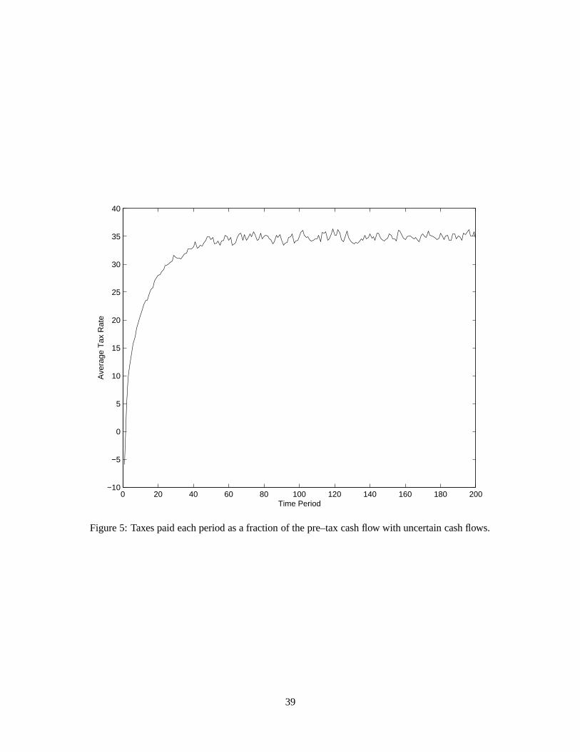
Figures 4 and 5 depict the time path of taxes paid. Figure 4 shows the taxes paid in each period, as a
fraction of the cash flow, under certainty, using Ct � 100, τp � 35%, and other parameters the same as in
Table 4. The taxes are small initially because of the tax shield supplied by the original basis. As shares
are repurchased, the share price grows, and the tax shield from the basis becomes negligible. Within 50
periods, the flows are being taxed at close to the full 35% rate. Figure 5 shows that with uncertainty and
the possibility of negative cash flows a similar pattern emerges. In it we plot the average taxes (under the
24

martingale measure) paid in each period, across sample paths in the simulation reported in the third line of
Table 4.
Finally, in Table 5 we provide information about the relative accuracy of our different methods of calcu-
lating or estimating the present value of the tax liability. When cash flows are positive, we can compare the
approximation in this section to the numerical solutions reported in Section 3. Similarly, for the certainty
case, we can compare both the numerical solution and the approximation to the closed-form solution. The
table shows that the approximation understates the present value of the tax liability, but this bias is of similar
magnitude to the numerical errors associated with the methods from Section 3.
Cash Flow OutcomesC 100 � 100 D C 120 � 60 DApprox. Numerical Closed-Form Approx. Numerical
Panel A: Tax rate of 28%Value 1,407.99 1,404.81 1,400.40 1,407.06 1,403.73Implicit tax rate (%) 15.52 15.71 15.98 15.58 15.78Cost of capital (%) 7.10 7.12 7.14 7.11 7.12Percent of PV taxes (%) 55.43 55.11 57.06 55.63 56.34
Panel B: Tax rate of 35%Value 1,336.15 1,328.39 1,323.70 1,336.09 1,327.71Implicit tax rate (%) 19.83 20.30 20.58 19.83 20.34Cost of capital (%) 7.48 7.53 7.55 7.48 7.53Percent of PV taxes (%) 56.66 57.99 58.79 56.67 58.11
Table 5: Cost of Capital and Implicit Tax Rates with Negative Cash Flows: The implicit tax rate is thatrate that, under full taxation would set the present value of the after–tax cash flows equal to their calculatedvalue. The cost of capital is the discount rate that sets the present value of of the pre–tax, expected cashflows equal to the calculated value. The percent of PV taxes is the present value of the of taxes paid, as apercentage of the the present value of the taxes paid under full taxation. taxes paid assuming fully taxeddividends. Calculations assume an after-tax discount rate of 6%, and that the probability of the higher cashflow is two-thirds. The simulations used to estimate the present value of taxes paid were carried out over200 periods, with 2,000 sample paths for each case. The column marked Approx. gives results obtainedby applying the numerical method described in Section 4, the column marked Numerical gives results fromapplying the recursive method described in Section 3 and the column marked Closed–Form gives the resultsfrom applying Equation 12.
25

4.2 Allowing for Growth
The approximation developed for calculating the present value of the personal tax liability can be adapted in
a straightforward manner to allow for growth in aggregate cash flows. Assume the firm’s cash flows follow
a geometric random walk with log-normal innovations, combined with a multiplicative shock to determine
the sign.
Ct � δt χt (43)
where
δt � δt � 1 exp µ 12
σ2 σεt � (44)
and χt is equal to 1 with probability q and � 1 with probability 1 � q. Suppose taxation is proportional
at rate τo. If the pricing kernel is also a geometric random walk with lognormal innovations, and χt is
independent of the pricing kernel, then the value of this process can be computed (see, for example, Berk,
Green and Naik (1999)) as:
Vt τo � � δt 2q � 1 � 1 � τo �1 � eµ QO� r (45)
where µ � is the risk-neutralized growth rate, which is computed by subtracting from µ a constant that depends
on the correlation between the innovations to the pricing kernel and δt . We take (45) to be the exogenous
process for firm value. We simulate this process, and, using (43) pre-tax cash flows. We compute the shares
repurchased, price per share, and taxes paid along each sample path. The are averaged and present valued,
to determine a PVTAX τo � . We then iterate on the tax rate to a solution to:
PVTAX τ � � � δt 2q � 1 � τ �1 � eµ Q � r (46)
Table 6 reports the results of these calculations. The number of sample paths used here is much higher
than in our earlier simulations because of the high variance associated with the random walk. The costs of
capital in this table should be interpreted as continuously compounded rates, in line with equation (45).
When contrasted with Table 4, it appears that adding growth has two effects. First, the firm’s share-
holders are more heavily taxed. The implicit tax rates and the ratio of the present value of taxes paid to the
present value of taxes under proportional taxation both are higher in Table 6. This is consistent with the
results for the certainty case, and is apparently due to the fact that the growth in the value of the firm and in
26

prices erodes the value of the tax shields from the basis more quickly.
Second, the various measures of the value of the tax liability in Table 6 are decreasing in the volatility
of the cash flows, σ. We should interpret increases in σ here as increases in idiosyncratic risk, as we are
holding the risk-neutralized growth rate fixed across columns in the table. In contrast, when expected cash
flows are perpetual, as in Table 4, the value of the tax liability increased in the volatility. This difference
appears to be due to the greater influence of the opportunity to pay negative taxes under the random walk
model. Since the cash flows are proportional to the value, which is growing, when negative cash flows occur
in this model it is more likely they will lead to large price drops below the basis of outstanding shares,
capital losses, and negative taxes. The simulations in Table 6 produce negative taxes 18-19% of the time,
for σ �R� 1, and 24-25% of the time for σ �R� 2. For the constant expected cash flow model from Table 4,
the simulations generate negative taxes only 11-12% of the time for all cases. The benefits of these capital
losses, in the case of the random walk model, dominate the other sources of concavity in the shareholders
after-tax payoff.
VolatilityFull tax σ � 0 � 1 σ � 0 � 2 No tax
Panel A: Tax rate of 28%Value 1,836.24 2,036.54 2,067.53 2,550.33Implicit tax rate (%) 28.00 20.15 18.93 0.00Cost of capital (%) 7.60 7.03 6.96 6.00Percent of PV taxes (%) 100.00 71.95 67.61 0.00
Panel B: Tax rate of 35%Value 1,657.71 1,903.72 1,932.46 2,550.33Implicit tax rate (%) 35.00 25.35 24.23 0.00Cost of capital (%) 8.22 7.40 7.31 6.00Percent of PV taxes (%) 100.00 72.44 69.22 0.00
Table 6: Cost of Capital and Implicit Tax Rates with Negative Cash Flows and Growth:The implicit taxrate is that rate that, under full taxation would set the present value of the after-tax cash flows equal to theircalculated value. The cost of capital is the discount rate that sets the present value of of the pre-tax, expectedcash flows equal to the calculated value. The percent of PV taxes is the present value of the of taxes paid, asa percentage of the the present value of the taxes paid under full taxation. taxes paid assuming fully taxeddividends. Calculations assume an after-tax discount rate of 6%, a risk-neutral growth rate of 2%, and thatthe probability of the a negative cash flow is two-thirds. The simulations used to estimate the present valueof taxes paid were carried out over 100 periods, with 20,000 sample paths for each case.
27

5 Conclusion
We analyze the advantages of equity financing by comparing the present value of the personal tax liability
of equity holders in a firm that distributes all cash through dividends to one that distributes cash through
repurchases. Under certainty, where the model admits a closed-form solution, we show this advantage is
quantitatively and economically substantial.
The magnitude of the personal-tax advantage to equity under uncertainty is similar to that under cer-
tainty. This has been shown using numerical methods to calculate the value of the tax liability when cash
flows are certain, and using a Monte Carlo approximation when cash flows are negative, and the firm must
issue new shares to finance shortfalls.
The tax advantages of equity at the personal level, in our model, are not sufficient to completely offset the
tax advantages of debt at the corporate level in the setting envisioned by M&M, where all payments to debt
are fully deductible. The personal tax advantages of equity do seem to be large enough to rationalize interior
capital structures when tax shields may be uncertain or redundant, or for plausible levels of bankruptcy
costs. When combined with estimates of the marginal tax benefits from debt financing that account for the
dynamics and redundant tax shields in corporate taxation, such as those in Graham (1998), our estimates
or elaborations of them might provide useful guidance regarding optimal capital structure and the corporate
cost of capital.
28

Appendix
Proofs
Proof of Lemma 1
Let C pt D ∞t � 1 be a conjectured sequence of equilibrium prices. Consider a shareholder with n shares,
and basis po. Suppose a potential buyer is willing to pay pt for these shares, and that this buyer’s optimal
realization strategy would be to sell n �t � s shares at date t s � s � 1 �������S� ∞, where ∑s n �t � s � n. Then it must
be the case that the price the buyer is willing to pay is less than the present value of after-tax receipts to the
buyer at the optimal strategy:
npt $ ∑s
n �t � s 1 r � s � pt � s � τp pt � s � pt � O� (A1)
The seller would accept the price pt only if the proceeds from the sale, net of the taxes paid,
n � pt � τp pt � po � (A2)
exceed the present value of after-tax cash flows from holding the shares and pursuing a realization strategy
that is optimal given basis po. Denote this value to the seller as V s po � . We will not show that, in fact, it
exceeds the after-tax proceeds from sale, (A2), which will establish the result. We know
V s po � � ∑s
n �t � s 1 r � s � pt � s � τp pt � s � po � � ∑s
n �t � s 1 r � s � pt � s � τp pt � s � pt � 8� ∑s
n �t � s 1 r � s τp pt � po ��npt � ∑
s
n �t � s 1 r � s τp pt � po �� npt � ∑s
n �t � sτp pt � po �� npt � nτp pt � po � � (A3)
The first line follows from the fact that the value to the seller under the seller’s optimal realization strategy
29

must be at least as high as under the buyer’s optimal strategy. The third line reflects the fact that the value
under the buyer’s optimal strategy exceeds the current, conjectured price by (A1). The fourth line follows
since the conjectured price exceeds the basis, and thus the taxes paid today exceed their present value if
deferred. This inequality is strict if the interest rate is positive. The last line is the after-tax proceeds from
sale, which establishes the result.
Proof of Proposition 1
With dividends, we can now write the value process as follows. At the ex-distribution date:
V et � C 1 � τp �
r�
At the cum-distribution point it is:
V ct � C 1 � τp �� C 1 � τp �
r�
Thus, the personal taxation enters the valuation proportionally. The stock price is just the above values
divided by the constant number of shares, so that the price drops with each distribution by the per-share,
after-tax value of the distribution:
pct � pe
t � C 1 � τp �n0
� (A4)
When all capital gains, realized or unrealized, are taxed each period, the share price grows, and the
number of shares shrink, at the pre-tax discount rate of r �� 1 � τp � . At the beginning of each tax period,
the shareholder’s basis is the current price. This basis is independent whether the shareholder is a buyer,
establishing a new basis, or a seller. Thus, any shareholder will be indifferent between receiving p t for her
shares, or holding them for one more period to receive value of
11 r
pt � 1 1 � τp �� τp pt � �
30

Equating this quantity to pt gives a difference equation for the price,
pt � 1 � pt
1 r
1 � τp � �If aggregate ex-distribution equity value is constant through time, then ptnt � pt � 1nt � 1, and the number of
shares must evolve as
nt � 1 � nt
1 r1 � τp
�This aggregate value will be
Vt � C 1 � τp �r
if we can show that, under the above laws of motion for the price and the number of shares, the aggregate
taxes paid by the equity holders under repurchase do, in fact, equal Cτ p. The aggregate tax liability at time
t is given by
nt � 1τp pt � pt � 1 � � τp T nt � 1 pt � 1
1 r
1 � τp � � nt � 1 pt � 1 U� τpnt � 1 pt � 1r
1 � τp� (A5)
At date t � 1 the cash distributed in a repurchase must be equal in value to the shares repurchased, so
C � pt � 1 nt � 2 � nt � 1 �� pt � 1 T nt � 1
1 r
1 � τp � � nt � 1 U� pt � 1nt � 1r
1 � τp� (A6)
Comparing (A5) to (A6) we see that the aggregate tax liability of the equity holders is, indeed, equal to
τpC.
Proof of Proposition 2
The initial value of the firm, equation (12) follows by taking the present value of the cash flows in
equation (10) as in the text. Equation (13) follows by substituting equation (12) into the solution for the
31

price at time t, equation (9). Substituting equation (13) into the cash constraint, equation (6) and solving for
the number of shares repurchased at time time t gives
nt � 1 � nt � Cpt� C
C �� 1 r � t � τp WV ∑∞s � 1
1X1 � r Y s � τp Z� 1 1 r � t � τp � ∞
∑s � 1
1 1 r � s � τp � � 1 � (A7)
The number of shares remaining at time t is given by nt � 1 � ∑∞s � t nt � 1 � nt � , and using equation (A7), this
is equal to
nt � 1 � ∞
∑s � t
1 1 r � s � τp � ∞
∑s � 1
1 1 r � s � τp � � 1
thus proving equation (14). Equation (15) follows from multiplying equations (14) and (15). To take the
limit, multiply and divide the value of the firm by 1 �� 1 r � t � 1 to get
Vt � C :[ 1 r � t � τp = ∞
∑s � t
1 1 r � s � τp� C : 1 r � � τp �� 1 r � t � 1 = ∞
∑s � 1
1 1 r � s � τp �� 1 r � t � 1 �Taking the limit as t � ∞,
limt � ∞
Vt � limt � ∞
C :B 1 r � � τp �� 1 r � t � 1 = ∞
∑s � 1
1 1 r � s � τp �� 1 r � t � 1� C 1 r � ∞
∑s � 1
1 1 r � s� Cr C �
Proof of Lemma 2 This follows from inspection of equation (22).
32

References
Bailey, Martin J. (1969), “Capital Gains and Income Taxation,” in Taxation of Income from Capital, A
Harberger and M. Bailey, eds., Washington: Brookings Institution.
Balcer, Yves, and Kenneth L. Judd, “Effects of Capital Gains Taxation on Lifecycle Investment and Portfolio
Management,” Journal of Finance, 42, pp. 743-757.
Berk, Jonathan, Richard C. Green and Vasant Naik (1999), “Valuation and Return Dynamics of R&D Ven-
tures,” working paper, University of California at Berkeley.
Brealey, R. A. and S. C. Myers (1996), Principles of Corporate Finance, McGraw-Hill, Inc.
DeAngelo, Harry, and Ronald Masulis (1980), “Optimal Capital Structure under Corporate and Personal
Taxation,” Journal of Financial Economics, 8:3-29.
Graham, John (1996), “Debt and the Marginal Tax Rate,” Journal of Financial Economics, 41:41-73.
Graham, John (1998), “How Big are the Tax Benefits of Debt,” working paper, Duke University.
Jensen, Michael, and William Meckling (1976), “Theory of the Firm: Managerial Behavior, Agency Costs
and Ownership Structure”, Journal of Financial Economics, 4: 305–360.
Leland, Hayne (1998), “Agency Costs, Risk Management, and Capital Structure”, Journal of Finance, 53:
1213–1244.
Miller, Merton (1977), “Debt and Taxes,” Journal of Finance, 32:261-275.
Modigiani, Franco, and Merton Miller (1963), “Corporate Income Taxes and the Cost of Capital: A Correc-
tion,” American Economic Review, 53:433-443.
Moyen, Nathalie (1999) “Investment Distortions Caused by Debt Financing” working paper, University of
Colorado at Boulder.
Myers, Stewart (1977), “Determinants of Corporate Borrowing”, Journal of Financial Economics, 5: 147–
175.
33

Parrino, Robert and Michael Weisbach (1999), “Measuring Investment Distortions Arising from
Stockholder–Bondholder Conflicts,” Journal of Financial Economics, 53: 3–42.
Poterba, James M. (1999), “Unrealized Capital Gains and the Measurement of After-Tax Portfolio Perfor-
mance,” Journal of Private Portfolio Management, Spring 1999, pp. 23-34.
34

0 5 10 15 20 25 30 35 4050
52
54
56
58
60
62
Personal Tax Rate
Per
cent
age
Tax
es: R
epur
chas
es to
Div
iden
ds
Figure 1: Present value of taxes paid, as a fraction of the value of the tax liability under full taxation of allequity flows, plotted against the personal tax rate. The three curves are associated with different values ofthe pre–tax discount rate, 3% (+), 6% (*) and 9% (x).
35

0 5 10 15 20 25 30 35 406
6.5
7
7.5
8
8.5
9
9.5
10
Personal Tax Rate
Cos
t of E
quity
Cap
ital
Figure 2: The cost of equity capital under certainty assuming an after–tax return of 6%, plotted againstthe personal tax rate. The solid line is the cost of equity capital C
p0. The dashed line is the cost of capital
prevailing when distributions are paid as dividends, r1 � τp
.
36

20 30 40 50 60 70 8010
15
20
25
30
35
40
45
Personal Tax Rate
Cor
pora
te T
ax R
ate
Figure 3: Corporate tax rates at which the firm is indifferent between debt and equity financing, assumingthat all distributions to equity are made through repurchases. At a given personal tax rate, for corporate taxrates above the curve plotted in the figure, the firm would prefer debt to equity financing.
37

0 20 40 60 80 100 120 140 160 180 200−10
−5
0
5
10
15
20
25
30
35
40
Time Period
Tax
Rat
e
Figure 4: Taxes paid each period as a fraction of the pre–tax cash flow under certainty.
38
0 20 40 60 80 100 120 140 160 180 200−10
−5
0
5
10
15
20
25
30
35
40
Ave
rage
Tax
Rat
e
Time Period
Figure 5: Taxes paid each period as a fraction of the pre–tax cash flow with uncertain cash flows.
39