The Pacific/Indian Ocean pressure difference and its

The Paci� c/Indian Ocean pressure difference and itsin� uence on the Indonesian Seas circulation: Part II—The

study with speci� ed sea-surface heights

by Vladimir M. Kamenkovich1, William H. Burnett2, Arnold L. Gordon3

and George L. Mellor4

ABSTRACTIn Part II we construct new numerical solutions to further analyze our results in Part I (Burnett et

al., 2003), that indicate the lack of a unique relationship between the Paci� c/Indian Ocean pressuredifference and the total transport of the Indonesian Through� ow (ITF). These new solutions involveperturbations of the sea level relative to the original solutions. We present detailed analyses of theoverall momentum and energy balances for these new solutions to stay consistentwith the proceduresdeveloped in Part I. The results validate our conclusions regarding the lack of a unique relationshipbetween the pressure head and the value of the total transport of the ITF. However, based on resultsfrom all the experiments, we have found that the seasonal variations of the total transport of the ITFare in phase with the pressure-head variations. Thus the hypothesis by Wyrtki (1987) that thepressure head, measured by the sea-surface-height difference between Davao (Philippines) andDarwin (Australia), is well correlated with the total transport is qualitativelysupported.

1. Introduction

In Part I (Burnett et al., 2003) we discussed the in� uence of the Paci� c-Indian Oceanpressure difference on the Indonesian Seas Through� ow (ITF). We showed strongevidence that external factors—the components of the pressure head (XEPRH andYEPRH) and the local wind stress (WUSURF and WVSURF)— did not uniquely deter-mine the value of the total transport of the ITF. Other factors, such as the componentsof thebottom form stress (XBTS and YBTS), the components of the internal pressure head(XIPRH and YIPRH) and the total in� ow and out� ow transports caused by the MindanaoCurrent, North Equatorial Counter Current, and New Guinea Coastal Current were alsoimportant (see Appendix A for an explanation of the acronyms).

To derive these conclusionswe analyzed the momentum and energy balances for a series

1. Department of Marine Sciences, University of Southern Mississippi, Stennis Space Center, Mississippi,39529, U.S.A. email: [email protected]

2. Naval Meteorology and Oceanography Command, Stennis Space Center, Mississippi, 39529, U.S.A.3. Lamont Doherty Earth Observatory of Columbia University, Palisades, New York, 10964, U.S.A.4. Program in Atmospheric and Oceanic Sciences, Princeton University, Princeton, New Jersey, 08544,U.S.A.

Journal of Marine Research, 61, 613–634, 2003

613

of experiments with prescribed seasonally varying total transports through four open ports(Type I experiments). The � rst objective of Part II is to prove the robustness of these resultsby performing a series of special experiments with perturbed pressure heads. Then weanalyze their impact on the Indonesian Seas circulationpattern and the total transport of theITF. In these experiments we prescribe seasonally varying sea-surface heights at the openports rather than the total transports, and we will refer to such experiments as Type IIexperiments.

The second objective of Part II is to analyze whether some relation between seasonalvariations of the pressure head and the total transport of the ITF exists or not. Although aunique relation between the pressure head and the total transport of the ITF is lacking,nonetheless a correlation between their seasonal variations could in principle exist. Thisobjective arose from Wyrtki’s (1987) hypothesis on the correlation of the pressure head,measured by the sea-surface-height difference between Davao (Philippines) and Darwin(Australia), and the total transport of the ITF. We will address this question by combiningthe results of the Type I and Type II experiments and analyzing the variations of thedifferent measures of the pressure head.

2. The Type II experiments

In Part I we ran Type I experiments with seasonally varying, normal and tangentialvelocities prescribed at four open ports. In Part II we will run Type II experiments with thesame model con� guration but with different boundary conditionsby specifying sea-surfaceheights and tangential velocities at the four open ports (refer to Appendix B for details).

To check the robustness of the results in Part I we consider Type II experiments of aspecial kind. First, we specify the initial sea-surface height for the Type II experiment, hII

(i),as the sum of the output of the corresponding annual-mean Type I experiment, hI

(i), and asea-surface-height perturbation, hd. The perturbation, hd, is introduced in the followingway. We divide the model domain into the three partitions IO (0 , I , 45), IS (46 , I ,

149), and PO (150 , I , 250) shown schematically in Figure 1. Within the IO and POpartitions we specify constant values of hd 2 hIO and hPO respectively—while within theIS partition we prescribe a linear interpolation between hIO and hPO. The domain integralof hd is then set to zero (the mass conservation constraint) to establish a relation betweenhIO and hPO. Thus the parameter hPO will be a free variable.

Second, we specify the sea-surface height at the open ports, hII(b), as the sum of the

output of the seasonally varying Type I experiment at the ports, hI(i), and the perturbation

hd (see the formulation of numerical boundary conditions in Appendix B). The perturba-tion hd does not change in time. Tangential velocities at the ports are taken from the Type Iexperiment output without any perturbation while, at the closed part of the boundary wespecify no-slip boundary conditions. We ramped the model during the � rst 30 computa-tional days to reduce the impact of transients, and the model reached a seasonally varying

614 [61, 5Journal of Marine Research

state within one computational year. Only two computational years of simulation arerequired for these experiments.

We ran two Type II experiments by setting the sea-surface-height perturbation in thePaci� c, hPO, equal to constant value 12.5 mm (Type IIA experiment) or to 22.5 mm(Type IIB experiment) for all seasons. The effect of local winds was not taken into accountfor these experiments, however we did analyze the effect of local winds in Part I. The TypeIIA experiment should increase the pressure head between the two oceans while the TypeIIB experiment should decrease the pressure head. Note that the total transport of the ITF isnot prescribed for any Type II experiment.

A perturbation of 2.5 mm might seem extremely small for the Indonesian Seas area butthis is a barotropic elevation. For a crude estimate of the relation between scales of h inbarotropic and baroclinic motions, suppose that the depth-integrated velocities in bothmodels are on the same order. Then, Ubc

(s)h ’ UbtH, (for example, if U ’ Ubc(s) exp( z/h)

then *2H0 Udz ’ Ubc

(s)h since H .. h), where Ubc(s) is the typical baroclinic velocity at the

sea surface and h is the typical vertical scale for the baroclinic motion; Ubt is the typicalvelocity for a barotropic motion; and H is the depth of the ocean. Thus, Ubc

s /Ubt ’ H/h

Figure 1. Schematic of the 250 3 250 model domain with the locationsof the three partitions IO, IS,and PO.

2003] 615Kamenkovich et al.: The study with speci� ed sea-surface heights

and from geostrophic relations near the sea surface, it follows that hbc/hbt ’ H/h, wherehbc and hbt are the typical values of the sea-surface height for baroclinic and barotropicmotions respectively. Finally, if H/h ; 10 then hbc/hbt are also on the order of 10.Therefore, a perturbation of 10 mm in a barotropic model can be considered equivalent to a10 cm perturbation in a baroclinic model.

The geostrophic relations apply at the four open ports (Burnett et al., 2000; Fig. 1).Therefore, the perturbation, hd, in the Type IIA/B experiments was speci� ed in a way thatdid not change the pressure gradient across the entrances of the open ports. If we succeed inconstructing such solutions, we will � nd circulation patterns with noticeably distinctpressure differences between the Paci� c and Indian Ocean, and very small variations in the

Figure 2. The boreal summer horizontal velocity patterns (m/s) for the Type IIA (a) and IIB (b)experiments.


total transports at the open ports. Small variations could be caused by some ageostrophiceffects at the open ports, which should be present, for example, due to the placement of theequator near the southern end of the New Guinea Coastal Current (NGCC) port. InAppendix B we further outline the method for constructing Type IIA/B solutions.

Figure 2a,b provide the boreal summer horizontal velocity pattern for the Type IIA andType IIB experiments, respectively (all seasons discussed in this paper are relative to theNorthern Hemisphere), and are representative of other seasons (see Burnett, 2000). Thesummer total transports through eight selected passageways and four open ports for allexperiments are provided in Table 1. The transport through the Indian Ocean open port isthe total transport of the ITF. In the Type IIA experiment, the total transport of the ITFincreases compared to the Type I experiment, as does the transport through the eight

Figure 2. (Continued)


passageways (labeled A through H in Fig. 1 of Part I). The NECC out� ow port is the onlyopen port where the transport through the port is reduced. Throughout the model grid, thehorizontal velocity vector magnitudes are larger, however, the velocity directions do notchange. Alternatively, for the Type IIB experiment, the total transport of the ITF and thetransport through the eight passages decrease. The velocity vectors, throughout the grid,are also smaller and do not change direction.

Figure 3a,b provide the Type II A/B experiment sea-surface heights for the summer(representative of other seasons, see Burnett, 2000). The perturbation of the sea-surfaceheight in the boundary conditions leads to signi� cant changes of the sea-surface heightthroughout the whole domain. Results from the Type IIA experiment show that highersea-surface heights occur throughout the Paci� c Ocean and lower heights occur in theIndian Ocean, compared to the Type I experiment (see Fig. 6, Part I), qualitativelyindicating that the pressure difference increased between the two oceans. Similarly, resultsfrom the Type IIB experiment show that lower (higher) sea-surface heights occurthroughout the Paci� c (Indian Ocean) indicating that the pressure difference decreasedbetween the two oceans. In the next section we will conduct a quantitative analysis of themomentum and energy balances of the Type IIA/B experiments.

3. The momentum and energy balances

In Part I (Burnett et al., 2003) we discussed in detail the overall momentum and energybalances for the series of experiments with the prescribed seasonally varying totaltransports through the open ports. A similar analysis for the new series of the Type IIA/B

Table 1. The absolutevalues of the total transports through the four open ports and eight passages forthe Type I and Type IIA/B experiments during summer.

PassageType I(Sv)

Type IIA(Sv)

Type IIB(Sv)

Indian Ocean (out� ow) or ITF 20.0 22.9 17.9New Guinea Coastal Current (in� ow) 19.0 19.8 18.5North Equatorial Countercurrent (out� ow) 25.0 23.6 25.6Mindanao Current (in� ow) 26.0 26.7 25.0Makassar Strait (A) 6.4 7.4 5.7Molucca Sea (B) 10.9 12.6 9.6Halmahera Sea (C) 3.1 3.4 2.9Lombok Strait (D) 4.5 5.1 4.1Sumba Strait (E) 3.6 4.3 3.1Flores Sea (F) 0.9 1.0 0.7Ombai Strait (G) 9.4 10.8 8.3Timor Sea (H) 5.1 5.7 4.6

Refer to Part I, Figure 1 for locations of the ports and passageways.


Figure 3. The boreal summer sea surface heights (m) for the Type IIA (a) and IIB (b) experiments.


experiments with the prescribed seasonally varying sea-surface heights at the open portsbasically supports the conclusions of Part I. We will brie� y review the main results of theexperiments without local wind-stress effects. Table 2 provides the overall x-momentumbalance terms for each season for the Type I and Type IIA/B experiments. As in Type Iexperiment the overall x-momentum balance is basically reduced to the overall geostrophicbalance:

XCOR 5 XPGRD, (1)

where, XCOR is the x-component of the Coriolis force and the x-component of thepressure gradient XPGRD is,

XPGRD 5 XEPRH 1 XIPRH 1 XBTS. (2)

In our experiments with realistic topography the x-component of the resultant of pressureforces acting on the � uid at the internal side boundaries (XIPRH) appeared negligiblysmall. The x-component of the resultant of pressure forces acting on the � uid at theexternal side boundaries (XEPRH) in the experiment IIA is larger than in the experimentIIB. In both experiments, IIA and IIB, the x-component of the bottom form stress (XBTS)is signi� cantly larger than XPGRD, thus stressing the importance of XBTS in determiningthe total transport of the ITF. Note that the momentum balance terms are at their highestvalues during the summer, and lowest during the winter, which should be expected sincethe model highest and lowest transport values occur during the summer and the winter,respectively.

Table 2. The domain integral x-momentum balance terms for the Type I and Type IIA/B experiments.Refer to Appendix A for the term de� nitions.

Season(dimensions) Type

Coriolis(XCOR)

1 3 109m4s22

Pressuregradient

(XPGRD)1 3 109m4s22

Totalpressure head

(XPRH)1 3 109m4s22

Externalpressure head

(XEPRH)1 3 109m4s22

Bottomform stress

(XBTS)1 3 109m4s22

SSHdifference(SSHDIF)

1 3 1022m

I 0.38 3 1022 0.10 3 1021 20.30 20.29 0.31 20.96Winter IIA 20.75 3 1021 20.73 3 1021 20.54 20.54 0.47 21.47

IIB 0.79 3 1021 0.82 3 1021 20.77 3 1021 20.83 3 1021 0.16 20.46

I 20.23 20.23 20.97 20.96 0.74 22.43Spring IIA 20.31 20.32 21.22 21.21 0.91 22.98

IIB 20.16 20.17 20.75 20.75 0.59 21.96

I 20.45 20.46 21.65 21.64 1.19 23.97Summer IIA 20.54 20.55 21.92 21.91 1.37 24.57

IIB 20.39 20.40 21.44 21.44 1.05 23.53

I 20.19 20.19 20.93 20.92 0.74 22.45Fall IIA 20.28 20.28 21.19 21.18 0.92 23.01

IIB 20.13 20.13 20.72 20.72 0.60 21.98


The overall geostrophic approximation is valid for the y-momentum balance (seeTable 3). Therefore:

YCOR 5 YPGRD, (3)

where,

YPGRD 5 YEPRH 1 YIPRH 1 YBTS. (4)

Contrary to the overall x-momentum balance, the y-component of the resultant ofpressure forces acting on the � uid at the internal side boundaries (YIPRH) becomesnoticeable. Hence, we � nd another factor important for determining the total transport ofthe ITF. As in the x-momentum balance, y-momentum balance terms are at their highestvalues during the summer, and lowest during the winter.

The overall energy balance terms for the Type I and Type IIA/B experiments arepresented in Table 4 for each season. The sum of kinetic and potential energies integratedover the total � uid volume (TENER) for the Type IIA experiment is higher than thecorresponding value for the Type I experiment for each season, while TENER for the TypeIIB experiment is lower than the corresponding value for the Type I experiment. For allexperiments TENER is higher in the summer and lower in the winter, which is expectedsince the model was developed with the highest transports in the summer and lowesttransports in the winter. During each season, the total kinetic energy (the kinetic energyintegrated over the total � uid volume) is larger than the total potential energy (approxi-mately by a factor of two or three for the spring, summer, and fall). For all experiments thetotal work (per unit time) performed by the pressure forces at the four ports (-PREWK) is

Table 3. The domain integral y-momentum balance terms for the Type I and Type IIA/B experiments.Refer to Appendix A for the term de� nitions.


Coriolis(YCOR)

1 3 109m4s22

Pressuregradient

(YPGRD)1 3 109m4s22

Totalpressure head

(YPRH)1 3 109m4s22

Externalpressure head

(YEPRH)1 3 109m4s22

Bottomform stress

(YBTS)1 3 109m4s22

I 0.43 0.43 0.23 0.20 0.20Winter IIA 0.48 0.48 0.16 0.10 0.32

IIB 0.38 0.38 0.31 0.29 0.71 3 1021

I 0.58 0.57 0.12 0.44 3 1021 0.45Spring IIA 0.62 0.61 0.45 3 1021 20.53 3 1021 0.57

IIB 0.52 0.52 0.20 0.14 0.32

I 0.75 0.74 0.42 3 1021 20.81 3 1021 0.70Summer IIA 0.79 0.78 20.32 3 1021 20.17 0.81

IIB 0.69 0.68 0.12 0.19 3 1021 0.56

I 0.62 0.61 0.18 0.10 0.43Fall IIA 0.67 0.66 0.11 0.11 3 1021 0.55

IIB 0.57 0.56 0.26 0.20 0.31


basically balanced by the total work (per unit time) performed by the horizontal and bottomfriction forces (HFWK and BFWK). So the approximate form of the overall energy balanceis

PREWK 5 HFWK 1 BFWK. (5)

In Part I, we performed an additional Type I experiment by setting the bottom depth to aconstant value of 4500 m. We found that the bathymetry had a profound in� uence on thedirection and magnitude of the ITF. Analogously we performed a similar Type IIAexperiment. Figure 4 shows that the horizontal velocity pattern for the Type II experimentis similar to the Type I experiment, with the ITF � owing along the western boundary,through the Makassar and Lombok Straits, and exiting through the IO open port. Thevelocity vectors increase in magnitude, compared to the Type I case; however, the vectordirections do not change. Therefore, changing the pressure head when the bottom formstress is eliminated does not change the direction of the ITF.

The integral momentum and energy balance relations (1)–(5) are also valid for theconstant depth case. When XBTS and YBTS were set to zero, the pressure head, XEPRH,changed by 68% relative to the Type I experiment. The open port transports, QMC, QNECC,and QNGCC changed in the Type IIA experiments, relative to those of the Type Iexperiment, by approximately 5%; however, for QIO, the change reached 26%. Thetransports through the Makassar, Sumba, Ombai Straits, and the Flores and Timor Seas for

Table 4. The domain integral energy balance terms for the Type I and Type IIA/B experiments.Refer to Appendix A for the term de� nitions.


Kinetic andpotential

energy sum(TENER)

1 3 109m5s22

Work ofpressure forces

(PREWK)1 3 106m5s23

Work ofhorizontal friction

(HFWK)1 3 106m5s23

Work ofbottom friction

(BFWK)1 3 106m5s23

I 1.40 20.76 20.72 20.66 3 1021

Winter IIA 2.31 21.13 21.09 20.14IIB 0.90 20.50 20.51 20.38 3 1021

I 4.29 22.39 21.88 20.35Spring IIA 6.00 23.39 22.59 20.59

IIB 3.09 21.71 21.38 20.21

I 9.68 25.65 24.14 21.19Summer IIA 12.29 27.30 25.27 21.69

IIB 7.99 24.58 23.44 20.89

I 4.72 22.49 22.13 20.41Fall IIA 6.52 23.46 22.90 20.66

IIB 3.54 21.79 21.63 20.26


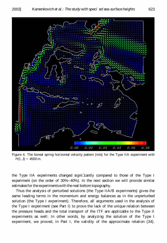
the Type IIA experiments changed signi� cantly compared to those of the Type Iexperiment (on the order of 30%–40%). In the next section we will provide similarestimates for the experiments with the real bottom topography.

Thus the analysis of perturbed solutions (the Type IIA/B experiments) gives thesame leading terms in the momentum and energy balances as in the unperturbedsolution (the Type I experiment). Therefore, all arguments used in the analysis ofthe Type I experiment (see Part I) to prove the lack of the unique relation betweenthe pressure heads and the total transport of the ITF are applicable to the Type IIexperiments as well. In other words, by analyzing the solution of the Type Iexperiment, we proved, in Part I, the validity of the approximate relation (34).

Figure 4. The boreal spring horizontal velocity pattern (m/s) for the Type IIA experiment withH(I, J) 5 4500 m.


This implies that the total transport of the ITF depends on the pressure head andon the bottom form stress; on the internal pressure head; and on transports QIO,QMC, QNECC, and QNGCC. Now we see that the same relation is true for “close”solutions (the Type IIA/B experiments). This con� rms the robustness of the relation(34) in Part I.

4. The seasonal variations of the pressure heads and the through-the-ports totaltransports

In Part I, four proxies were used to quantitatively measure the pressure head. They arethe x- and y-components of the resultant of pressure forces acting on the � uid at theexternal side boundaries (XEPRH and YEPRH); the total work (per unit time) performedby the pressure forces at the four ports (PREWK), and the sea-surface height differencebetween a point in the Paci� c and a point in the Indian Ocean (SSHDIF). In Figure 5 wepresent the seasonal variation of all four measures of the pressure head for the Type I andthe Type IIA/B experiments. All characteristics vary in-phase with each other. The highestvalues of XEPRH, PREWK, and SSHDIF for both the Type I and Type II experimentsoccur during the boreal summer when the total transport of the ITF is highest; the lowestduring the winter. The Type I values are between the Type IIA and Type IIB values. Allvalues of XEPRH, SSHDIF, and PREWK are negative in accordance with the direction ofthe ITF (out� ow through the IO port). Therefore, the absolute values of these characteris-tics are larger for the Type IIA experiments and smaller for the Type IIB experiments(relative to the values of the Type I experiment). For the Type IIA experiment uXEPRHu isincreased on average approximately by 25%; uSSHDIFu— by 20%; and uPREWKu— by40%, and by much higher values for the winter. For the Type IIB experiment, uXEPRHu isdecreased by 20%; uSSHDIFu— by 16%; and uPREWKu—by 27%, and by much lowervalues for the winter. The values of YEPRH, however, change sign, although the variationof YEPRH is in-phase with that of XEPRH, SSHDIF, and PREWK. The deviations ofuYEPRHu for the Type IIA/B experiments are on the order of 60% relative to that value forthe Type I experiment.

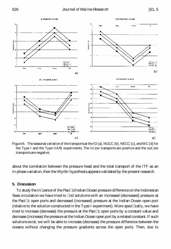
The seasonal variations of the total transports through the open ports, QIO, QMC, QNECC,and QNGCC, are given in Figure 6 (taking into account the appropriate sign). It is clearlyseen that the absolute values of all transports are increased for the Type IIA experiment anddecreased for the Type IIB experiments (relative to the corresponding value for the Type Iexperiment). Relative to the values of the Type I experiment, the corresponding values forthe Type IIA/B experiments, QMC, QNECC, and QNGCC, change by only 3%–5%. Thechanges of QIO for the Type IIA/B experiments, relative to that for the Type I experiment,is more signi� cant; they equal to 16%–19% in the spring, summer, and fall and reach 50%in the winter. Formally this is due to the fact that the variations of QMC, QNECC, and QNGCC

are arithmetically added to give more noticeable variation of QIO, so there is no violationofthe mass balance. It is worth noting that the variations of all transports are in-phase.


Note that we failed to make the relative change of QIO, as small as that of the other porttransports. But the relative changes of all the pressure-head measures appear morenoticeable as compared to the relative changes of the port transports. That gives anadditional point in favor of the conclusion for the lack of the unique relation between thepressure head and the total transport of the ITF.

Finally, we compare the seasonal variations of all measures of the pressure head and thetotal transport of the ITF for the Type I experiment (with and without local wind stresses)and the Type IIA/B experiments (Fig. 7). All variations are in-phase except for the Type Iexperiment with wind. When a local wind is included, XEPRH, YEPRH, and WUSURFchange similarly; however, the periods of their maximal variations do not coincide.Moreover the variations of SSHDIF, PREWK, and WVSURF are completely out of phasewith the variation of the pressure head. If we exclude this case and view Wyrtki’s idea

Figure 5. The seasonal variation of the various measures of the pressure head XEPRH (a), YEPRH(b), SSHDIF (c), and PREWK (d) for the Type I and the Type IIA/B experiments.


about the correlation between the pressure head and the total transport of the ITF as anin-phase variation, then the Wyrtki hypothesis appears validated by the present research.

5. Discussion

To study the in� uence of the Paci� c/Indian Ocean pressure difference on the IndonesianSeas circulation we have tried to � nd solutions with an increased (decreased) pressure atthe Paci� c open ports and decreased (increased) pressure at the Indian Ocean open port(relative to the solution constructed in the Type I experiment). More speci� cally, we havetried to increase (decrease) the pressure at the Paci� c open ports by a constant value anddecrease (increase) the pressure at the Indian Ocean open port by a related constant. If suchsolutions exist, we will be able to increase (decrease) the pressure difference between theoceans without changing the pressure gradients across the open ports. Then, due to

Figure 6. The seasonalvariation of the transportsat the IO (a), NGCC (b), NECC (c), and MC (d) forthe Type I and the Type IIA/B experiments. The in� ow transports are positive and the out� owtransports are negative.


geostrophy that exists at the entrances of the open ports, it is clear that the total transportsthrough the open ports will not substantially change, including the total transport throughthe IO port (the total transport of the ITF). Thus, different patterns of Indonesian Seascirculation would exist with suf� ciently distinct intra-ocean pressure differences andalmost the same total transport of the ITF. In other words, the pressure difference betweenthe Paci� c and Indian Ocean would not practically impact the value of the ITF totaltransport.

We thought that such solutions are dynamically possible. In fact, it seems reasonable toassume that the overall momentum and energy balance relations (1)–(5) will govern suchsolutions. Then any signi� cant change in the pressure heads (XEPRH and YEPRH) wouldbe balanced by the bottom form stress (XBTS and YBTS) and by the internal pressureheads (XIPRH and YIPRH) thus leading to the small changes of the total transport.Further, any signi� cant change of the PREWK would be balanced by the appropriate

Figure 7. The comparisonof the seasonalvariationof the (negative) total transportof the ITF, Q (Sv)and different measures of the pressure heads: XEPRH (m4 s22 ), SSHDIF (m), YEPRH (m4 s22 ),PREWK (m5 s2 3), WUSURF and WVSURF (m4 s22 ) for the Type I experiment with no wind (a),the Type I experiment with wind (b), and the Type IIA/B experiments (c and d). In case (b) weconsider the components of the wind stress integratedover the model domain.


change of HFWRK, which is determined by the velocity gradients rather than by thevelocity itself as in the case of the bottom friction.

To construct the Type-II-experiment solutions we recon� gured the regional barotropicmodel of Part I to specify the sea-surface heights at the open ports, rather than the totaltransports. Then we introduced the perturbed solutions with the perturbed constant valuesof the sea-surface height at the open ports.

As the preceding analysis has shown, we managed to � nd the solutions with noticeablechanges in the pressure head and almost the same total transport through the MC, NECC,and NGCC ports. But it appeared that the relative change of the transport through the IOport, exceeded the relative changes for the above-mentioned transports by a factor of 3,being at the same time on average smaller as compared to the relative changes of thepressure head. Why is that?

Figure 8a presents the normal velocities for the Type I and the Type IIA/B experimentsat the entrance of each open port for the boreal summer (representative of each season, seeBurnett, 2000). Recall that the geostrophic approximation was valid at all open portsexcept for parts of the NGCC open port where the equator crosses the port, and in thesouthern boundary of the IO open port where a computational western boundary layerdevelops (Burnett et al., 2000). It is possible that ageostrophic effects cause the distinctionbetween normal velocities at the port entrance of the Type IIA/B and Type I.

It is not improbable, however, that there are other reasons for the variation of the normalvelocitiesat the port entrance besides the ageostrophic effects. Mathematically the problemcorresponding to the Type II experiment appeared to be very complicated and we failed toreach the exact ful� llment of the boundary conditions within the mouth of the ports. Weapplied the method of a special relaxation to solve the problem (see Appendix B) andobtained an approximate solution with some deviations of the sea-surface heights in theports from the prescribed values. This is clearly seen in Figure 8b where the boreal summersea-surface heights are presented (representative of other seasons, see Burnett, 2000); thepro� les are not parallel, as they should be for the exact solution (especially for MC and IOports). It is conceivable that the problem considered has no solution at all and it is possibleto � nd a “close” solution to the one sought only. To illustrate this point consider a � owwhose dynamics is such that variations of the pressure along the � ow and across the� ow are connected (such a � ow exists; see, for example, a boundary layer currentgoverned by (15), Part I). Therefore by varying the pressure gradient along the � ow weinevitably vary the pressure gradient across the � ow. It is clear that the Type IIA/Bproblem for such a � ow has no solution. As to our case, we do not know whether thesought solution exists or not.

Nevertheless we consider the Type IIA/B experiment solutions to be very helpful instudying the two objectives formulated in the introduction of this paper. First, suchsolutions are interesting per se. Second, they are alternative solutions, closely related tosolutions of the Type I experiment. All the conclusions based on the analysis of the Type I


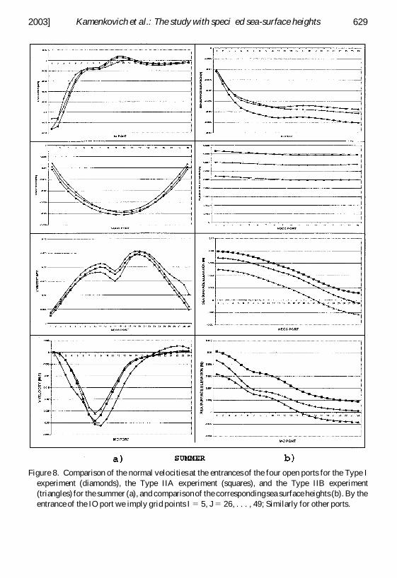
Figure 8. Comparison of the normal velocities at the entrances of the four open ports for the Type Iexperiment (diamonds), the Type IIA experiment (squares), and the Type IIB experiment(triangles) for the summer (a), and comparisonof the correspondingsea surface heights (b). By theentrance of the IO port we imply grid points I 5 5, J 5 26, . . . , 49; Similarly for other ports.


experiments are valid for these solutions as well. We have shown also that these solutionswill give additional credence to the conclusion for the lack of a unique relation between thepressure heads and the value of the total transport of the ITF.

6. Conclusion

Both of the objectives formulated in the Introduction have been met. First, thesolutions of the Type IIA/B experiments have been constructed and are considered tobe perturbations of the solution of the Type I experiment. We have shown the validityof the approximate relation (34) from Part I for the solutions of the Type IIA/Bexperiments. In other words, we con� rmed that the total transport of the ITF dependson the bottom form stress; on the internal pressure head; on the total transports throughthe Mindanao, North Equatorial Counter Current, and New Guinea Coastal Currentports and on the pressure head itself. This is true not only for the solution of the Type Iexperiment but for the “close” solutions of the Type IIA/B experiments as well.Through these experiments we were able to demonstrate the robustness of the relation(34), Part I. Moreover the comparison of the relative changes of all of the measures ofthe pressure head and the transports through the open ports showed the possibility ofthe existence of different Indonesian Seas circulation patterns with distinct inter-oceans pressure differences and almost the same total transport of the ITF. This pointgives additional credence to our main conclusion.

Second, we qualitatively con� rmed the hypothesis by Wyrtki (1987) about the correla-tion between the seasonal variation of the pressure head and the total transport of the ITF.We viewed the Wyrtki result as the in-phase variations of the pressure head and the totaltransport of the ITF. Potemra et al. (1997) and Lebedev and Yaremchuk (2000) alsosupport the pioneering result by Wyrtki (1987) with detailed analyses of the seasonalvariations of the total transport and the sea-surface height differences on the Paci� cand Indian Ocean sides of the Indonesian Seas area. This was con� rmed for all fourmeasures of the pressure head. Yet we note that the value of the total transport by itselfis not uniquely determined by any of the four measures of the pressure headintroduced.

The results of the Type I experiments with the local wind effects cannot be considered assupporting this conclusion. Some of the measures of the pressure heads are varied out ofphase while compared with the total transport. We think that this case needs moreinvestigationwithin the baroclinic model that is now in progress.

Acknowledgments. First of all, we would like to thank George Veronis for a very produc-tive discussion that resulted in the considerable clari� cation of several points of the paper. Theauthors gratefully acknowledge helpful advice from H. Hurlburt and D. Nechaev on differentaspects of the paper. The criticism of our three reviewers was very useful and allowed us tosubstantially modify the initial outline of the material. V. Kamenkovich was supported by NSF


grants OCE 96-33470 and OCE 01-18200. W. Burnett was supported by U.S. Navy funds.A. Gordon was supported by NSF grants OCE 00-99152 and OCE 96-33470. G. Mellor wassupported by NSF grant OCE 96-33470. The model analysis was supported by the Department ofDefense’s Major Shared Resource Center. The Naval Oceanographic Of� ce VisualizationLaboratory prepared the color graphics.

APPENDIX A

Frequently used terms

BFWK—the total work performed by the bottom friction forces (per unit time), see (40)Part I.

HFWK—the total work performed by the horizontal friction forces (per unit time), see (40)Part I.

ITF—Indonesian Through� owIO port—Indian Ocean open port (out� ow)MC port—Mindanao Current open port (in� ow)NECC port—North Equatorial Counter Current open port (out� ow)NGCC port—New Guinea Coastal Current open port (in� ow)PREWK—minus the total work performed by the pressure forces at the four ports (per unit

time), see (40) Part I.QIO—total transport through the IO port.QMC—total transport through the MC portQNECC—total transport through the NECC portQNGCC—total transport through the NGCC port.SSHDIF—the sea-surface height at the mouth of the IO port (I 5 5, J 5 49) minus the

sea-surface height at the mouth of the MC port (I 5 166, J 5 246). Introducedto imitate Wyrtki’s characteristic.

TENER—The sum of kinetic and potential energies integrated over the total � uid volume(see (40), Part I)

Type I experiment—Experiment with normal and tangential velocities prescribed at theopen ports and no slip boundary conditions at the closed part of theboundary

Type II experiment—Experiment with sea-surface-heights and tangential velocities pre-scribed at the open ports and no slip boundary conditions at theclosed part of the boundary

Type IIA experiment—Experiment with the boundary sea-surface-height values equal tothe corresponding output values from the Type I experiment plus aconstant perturbation of 2.5 mm at the MC, NECC, and NGCCopen ports in the Paci� c.

Type IIB experiment—the same as in Type IIA except minus a constant perturbation of2.5 mm at the Paci� c open ports.


WUSURF—the x-component of the wind stress integrated over the model domainWVSURF—the y-component of the wind stress integrated over the model domainXCOR—the x-component of the Coriolis acceleration integrated over the total � uid

volume (see (28) Part I)XBTS—the x-component of the resultant of pressure forces acting on the � uid at the

bottom (see (30) Part I)XEPRH—the x-component of the resultant of pressure forces acting on the � uid at the

external side boundaries (see (31), Part I)XIPRH—the x-component of the resultant of pressure forces acting on the � uid at the

internal side boundaries (see (32), Part I)XPGRD—the x-component of the pressure gradient integrated over the total � uid volume

(see (28) Part I)XPRH—the x-component of the resultant of pressure forces acting on the � uid at the side

boundaries of the domain, both external and internal (see (30), Part I)YCOR—the y-component of the Coriolis acceleration integrated over the total � uid

volume (see (35) Part I)YBTS—the y-component of the resultant of pressure forces acting on the � uid at the

bottom (see (36) Part I)YEPRH—the y-component of the resultant of pressure forces acting on the � uid at the

external side boundaries (see (37), Part I)YIPRH—the y-component of the resultant of pressure forces acting on the � uid at internal

side boundaries (see (38), Part I)YPGRD—the y-component of the pressure gradient integrated over the total � uid volume

(see (35) Part I)YPRH—the y-component of the resultant of pressure forces acting on the � uid at the side

boundaries of the domain, both external and internal (see (36), Part I)

APPENDIX B

Difference formulation

Refer to Appendix A of Part I (Burnett et al., 2003) for a description of the open portboundary conditions. Consider the IO open port (I 5 1, . . . , 5; 26 , J, ,49); other portsare handled similarly. We specify h(2, J) and V(2, J); calculate U(3, J) from thex-momentum equation by neglecting the horizontal friction and momentum advection; andset U(2, J) 5 U(3, J) as computational boundary conditions. A schematic is provided inFig. B.1.

Relaxation is applied within the open ports to suppress numerical noise followingMartinsen and Engedahl (1987). The relaxation procedure for the IO open port takes theform:

hn11(I, J) 5 a(I)hn11(2, J) 1 ~1 2 a(I))hn11(I, J) (B.1)


nn11(I, I) 5 a(I)nn11(2, J) 1 (1 2 a(I))nn11(I, J) (B.2)

un11(I, J) 5 a(I)un11(2, J) 1 (1 2 a(I))un11(I, J) (B.3)

for I 5 3; 4; 5 and 26 # J # 49, where hn11(I, J), un11(I, J), vn11(I, J) denote the value atn 1 1 time step; hn11(2, J) and vn1 1(2, J) are prescribed as boundary conditions whileun1 1(2, J) is taken from the boundary conditionof the Type I experiment; and hn1 1, un1 1,nn1 1 are calculated from the set of difference equations approximating the basic equations.The relaxation parameter, a(I); I 5 3, 4, 5; is equal to 0.028, 0.0028, and 0.00028. Such a

Figure B.1. The schematic of the speci� ed and calculated U, V, and h for the IO port (26 # J # 49)for I 5 2; 3; 4 for the Type II experiment. The prescribed sea surface heights h(2, J) and tangentialvelocities V(2, J) are denoted by black arrows and ovals. Normal velocities U(3, J) calculated byneglecting horizontal diffusion and momentum advection (a computational boundary condition)are denoted by partially � lled ovals. U(2, J) 5 U(3, J) is another computational boundarycondition,not shown here. Clear arrows and ovals denote variables that are calculatedby using thebasic equations of the Princeton Ocean Model as in Part I (Burnett et al., 2003).


procedure is equivalent to adding Newtonian friction to the basic equations, which in thedifference form (corresponding to relation (B.1)) is Ki [hn11(I, J) 2 hn11(2, J)], whereKi 5 ai/[(1 2 ai)Dt], Dt is the time step, and K(I) 5 0.002, 0.0002, and 0.00002 for I 5

3, 4, 5 (similarly for relations (B.2. and (B.3)). This procedure is analogous for the otherports.

It is important to stress that the physical interpretations from the numerical experimentswill be done within the operational domain: I 5 5, . . . , 246; J 5 2, . . . , 246. Thereforeh 5 h(5, J), J 5 26, . . . , 49; h 5 h(246, J), J 5 126, . . . , 144; h 5 h(246, J), J 5

176, . . . , 204; and h 5 h(I, 246), I 5 166, . . . , 189 will be considered as physicalboundary conditions for the sea surface elevation. The boundary conditions for h speci� edat I 5 2; I 5 249; and J 5 249 of the corresponding open ports will be referred to asnumerical ones.

To check that the outlined approach is working and will provide us with reasonablesolutions we ran a Type II experiment with the corresponding Type I experiment outputdata as boundary conditions at the open ports. The agreement with the Type I experimentwas satisfactory.

REFERENCESBurnett, W. H. 2000. A dynamical analysis of the Indonesian Seas Through� ow. Ph.D. dissertation,

Department of Marine Science, University of Southern Mississippi Press, Hattiesburg, MS,114 pp.

Burnett, W. H., V. M. Kamenkovich,A. L. Gordon and G. L. Mellor. 2003. The Paci� c/Indian Oceanpressure difference and its in� uence on the Indonesian Seas circulation: Part 1—The study withspeci� ed total transports. J. Mar. Res., 61, 577–611.

Burnett, W. H., V. M. Kamenkovich, D. A. Jaffe, A. L. Gordon and G. L. Mellor. 2000. Dynamicalbalance in the Indonesian Seas circulation.Geophys. Res. Lett., 27, 2,705–2,708.

Lebedev, K. V. and M. I. Yaremchuk. 2000. A diagnostic study of the Indonesian through� ow. J.Geophys. Res., 105(C5), 11,243–11,258.

Martinsen, E. A. and H. Engedahl. 1987. Implementationand testing of a lateral boundary scheme asan open boundary condition in a barotropicocean model. Coastal Eng., 11, 603– 627.

Potemra, J. T., R. Lukas and G. T. Mitchum. 1997. Large-scale estimation of transport from thePaci� c to the Indian Ocean. J. Geophys. Res., 102(C13), 27,795–27,812.

Wyrtki, K. 1987. Indonesian through� ow and the associated pressure gradient. J. Geophys. Res.,92(C12), 12,941–12,946.

Received: 21 August, 2001; revised: 9 September, 2003.


Documents

The Pacific/Indian Ocean pressure difference and its