The NLIN Procedure

Chapter 45The NLIN Procedure

Chapter Table of Contents

OVERVIEW . . . . . . . . . . . . . . . . . . . . . . . . . . . . . . . . . . .2373

GETTING STARTED . . . . . . . . . . . . . . . . . . . . . . . . . . . . . .2374

SYNTAX . . . . . . . . . . . . . . . . . . . . . . . . . . . . . . . . . . . . .2379PROC NLIN Statement . . . . . . . . . . . . . . . . . . . . . . . . . . . . .2380BOUNDS Statement . . .. . . . . . . . . . . . . . . . . . . . . . . . . . .2384BY Statement . . . . . . . . . . . . . . . . . . . . . . . . . . . . . . . . . .2385CONTROL Statement . .. . . . . . . . . . . . . . . . . . . . . . . . . . .2385DER Statements . . . . . . . . . . . . . . . . . . . . . . . . . . . . . . . . .2385ID Statement . . . . . . . . . . . . . . . . . . . . . . . . . . . . . . . . . .2386MODEL Statement . . . . . . . . . . . . . . . . . . . . . . . . . . . . . . .2386OUTPUT Statement . . . . . . . . . . . . . . . . . . . . . . . . . . . . . .2387PARAMETERS Statement. . . . . . . . . . . . . . . . . . . . . . . . . . .2389RETAIN Statement . . . . . . . . . . . . . . . . . . . . . . . . . . . . . . .2390Other Program Statements with PROC NLIN . . . . . . . . . . . . . . . . .2390

DETAILS . . . . . . . . . . . . . . . . . . . . . . . . . . . . . . . . . . . . .2391Automatic Derivatives . . . . . . . . . . . . . . . . . . . . . . . . . . . . .2391Hougaard’s Measure of Skewness .. . . . . . . . . . . . . . . . . . . . . .2394Missing Values . . . . . . . . . . . . . . . . . . . . . . . . . . . . . . . . .2394Special Variables . . . . . . . . . . . . . . . . . . . . . . . . . . . . . . . .2395Troubleshooting. . . . . . . . . . . . . . . . . . . . . . . . . . . . . . . . .2396Computational Methods .. . . . . . . . . . . . . . . . . . . . . . . . . . .2398Output Data Sets . . . . . . . . . . . . . . . . . . . . . . . . . . . . . . . .2403Confidence Intervals . . . . . . . . . . . . . . . . . . . . . . . . . . . . . .2403Parameter Covariance Matrix. . . . . . . . . . . . . . . . . . . . . . . . . .2404Reported Convergence Measures . .. . . . . . . . . . . . . . . . . . . . . .2405Displayed Output . . . . . . . . . . . . . . . . . . . . . . . . . . . . . . . .2406Incompatibilities with 6.11 and Earlier Versions of PROC NLIN . .. . . . . 2406ODS Table Names . . . . . . . . . . . . . . . . . . . . . . . . . . . . . . .2408

EXAMPLES . . . . . . . . . . . . . . . . . . . . . . . . . . . . . . . . . . .2409Example 45.1 Segmented Model . . . . . . . . . . . . . . . . . . . . . . . .2409Example 45.2 Iteratively Reweighted Least Squares . . .. . . . . . . . . . .2412Example 45.3 Probit Model with Likelihood function . .. . . . . . . . . . .2415

2372 � Chapter 45. The NLIN Procedure

REFERENCES . . . . . . . . . . . . . . . . . . . . . . . . . . . . . . . . . .2417

SAS OnlineDoc: Version 8

Chapter 45The NLIN Procedure

Overview

The NLIN procedure produces least squares or weighted least squares estimates ofthe parameters of a nonlinear model. Nonlinear models are more difficult to specifyand estimate than linear models. Instead of simply listing regressor variables, youmust write the regression expression, declare parameter names, and supply initialparameter values. Some models are difficult to fit, and there is no guarantee that theprocedure can fit the model successfully.

For each nonlinear model to be analyzed, you must specify the model (using a sin-gle dependent variable) and the names and starting values of the parameters to beestimated.

Using PROC NLIN, you can also

� confine the estimation procedure to a certain range of values of the parametersby imposing bounds on the estimates

� produce new SAS data sets containing predicted values, residuals, parameterestimates and SSE at each iteration, the covariance matrix of parameter esti-mates, and other statistics

� define your own objective function to be minimized

Estimation of a nonlinear model is an iterative process. To begin this process theNLIN procedure first examines the starting value specifications of the parameters.If a grid of values is specified, PROC NLIN evaluates the residual sum of squaresat each combination of parameter values to determine the set of parameter valuesproducing the lowest residual sum of squares. These parameter values are used forthe initial step of the iteration.


Then PROC NLIN uses one of these five iterative methods:

� steepest-descent or gradient method

� Newton method

� modified Gauss-Newton method

� Marquardt method

� multivariate secant or false position (DUD) method

These methods use derivatives or approximations to derivatives of the SSE with re-spect to the parameters to guide the search for the parameters producing the smallestSSE.

You can use the NLIN procedure for segmented models (see Example 45.1) or robustregression (see Example 45.2). You can also use it to compute maximum-likelihoodestimates for certain models (refer to Jennrich and Moore 1975; Charnes, Frome, andYu 1976).

Getting Started

The NLIN procedure performs univariate nonlinear regression using the least squaresmethod. Nonlinear regression analysis is indicated when you have information spec-ifying that the functional relationship between the predictor and response variablesis nonlinear in the parameters. Such information might come from direct knowledgeof the true model, theoretical developments, or previous studies.Nonlinear, in thissense, means that the mathematical relationship between the variables and parame-ters is not required to have a linear form. For example, consider the following twomodels:

Y = aX2 + b

Y =1

aX + b

wherea andb are parameters andX andY are random variables. The first model islinear in the parameters; the second model is nonlinear.

Estimating the Nonlinear ModelAs an example of a nonlinear regression analysis, consider the following theoreticalmodel of enzyme kinetics. The model relates the initial velocity of an enzymaticreaction to the substrate concentration.

f(x;�) =�1xi

�2 + xi; for i = 1; 2; : : : ; n

wherexi represents the amount of substrate forn trials andf(x;�) is the velocity ofthe reaction. The vector� contains the rate parameters.


Getting Started � 2375

Suppose that you want to study the relationship between concentration and velocityfor a particular enzyme/substrate pair. You record the reaction rate (velocity) ob-served at different substrate concentrations. Your data set is as follows:

data Enzyme;input Concentration Velocity @@;datalines;

0.26 124.7 0.30 126.9 0.48 135.9 0.50 137.60.54 139.6 0.68 141.1 0.82 142.8 1.14 147.61.28 149.8 1.38 149.4 1.80 153.9 2.30 152.52.44 154.5 2.48 154.7;

The SAS data setEnzyme contains the two variablesConcentration (substrate con-centration) andVelocity (reaction rate). The double trailing at sign (@@) in theINPUT statement specifies that observations are input from each line until all of thevalues are read.

The following statements request a nonlinear regression analysis:

proc nlin data=Enzyme method=marquardt hougaard;parms theta1=155

theta2=0 to 0.07 by 0.01;model Velocity = theta1*Concentration / (theta2 + Concentration);

run;

The DATA= option specifies that the SAS data setEnzyme be used in the analy-sis. The METHOD= option directs PROC NLIN to use the MARQUARDT iterativemethod. The HOUGAARD option requests that a skewness measure be calculatedfor the parameters.

The MODEL statement specifies the enzymatic reaction model

V =�1C

�2 + C

whereV represents the velocity or reaction rate andC represents the substrate con-centration.

The PARMS statement declares the parameters and specifies their initial values. Inthis example, the initial estimates in the PARMS statement are obtained as follows.Since the model is a monotonic increasing function inC, and

limC!1

��1C

�2 + C

�= �1

take the largest observed value of the variableVelocity (154.7) as the initial value forthe parameterTheta1. Thus, the PARMS statement specifies 155 as the initial valuefor Theta1, which is approximately equal to the maximum observed velocity.



To obtain an initial value for the parametertheta2, first rearrange the model equationto solve for�2:

�2 =�1C

V� C

By substituting the initial value ofTheta1 for �1 and taking each pair of observedvalues ofConcentration andVelocity for C andV , respectively, you obtain a set ofpossible starting values forTheta2 ranging from about 0.01 to 0.07.

You can choose any value within this range as a starting value forTheta2, or you candirect PROC NLIN to perform a preliminary search for the best initialTheta2 valuewithin that range of values. The PARMS statement specifies a range of values forTheta2, which results in a search over the grid points from 0 to 0.07 in incrementsof 0.01. The output from this PROC NLIN invocation are displayed in the followingfigures.

PROC NLIN evaluates the model at each point on the specified grid for theTheta2parameter. Figure 45.1 displays the calculations resulting from the grid search.

The NLIN ProcedureGrid Search

Dependent Variable Velocity

Sum oftheta1 theta2 Squares

155.0 0 3075.4155.0 0.0100 2074.1155.0 0.0200 1310.3155.0 0.0300 752.0155.0 0.0400 371.9155.0 0.0500 147.2155.0 0.0600 58.1130155.0 0.0700 87.9662

The NLIN ProcedureIterative Phase

Dependent Variable VelocityMethod: Marquardt

Sum ofIter theta1 theta2 Squares

0 155.0 0.0600 58.11301 158.0 0.0736 19.70172 158.1 0.0741 19.66063 158.1 0.0741 19.6606

NOTE: Convergence criterion met.

Figure 45.1. Nonlinear Least Squares Grid Search from the NLIN Procedure

The parameterTheta1 is held constant at its specified initial value of 155, the grid istraversed, and the residual sums of squares are computed at each point. The “best”


Getting Started � 2377

starting value is the point that corresponds to the smallest value of the residual sumof squares. Figure 45.1 shows that the best starting value forTheta2 is 0.06. PROCNLIN uses this point as the initial value forTheta2 in the following iterative phase.

PROC NLIN determines convergence using the relative offset measure of Bates andWatts (1981). When this measure is less than10�5, convergence is declared. Figure45.1 displays the iteration history.

The NLIN Procedure

Estimation Summary

Method MarquardtIterations 3R 5.861E-6PPC(theta2) 8.569E-7RPC(theta2) 0.000078Object 2.902E-7Objective 19.66059Observations Read 14Observations Used 14Observations Missing 0

Figure 45.2. Estimation Summary from the NLIN Procedure

Figure 45.2 displays a summary of the estimation including several convergence mea-sures R, PPC, RPC, and Object.

The R measure is the relative offset convergence measure of Bates and Watts. A PPCvalue of 8.569E-7 indicates that the parameterTheta2 (which has the largest PPCvalue of all the parameters) would change by that relative amount were PROC NLINto take an additional iteration step. The RPC value indicates thatTheta2 changed by0.000078, relative to its value in the last iteration. The Object measure indicates thatthe objective function value changed 2.902E-7 in relative value from the last iteration.

The NLIN Procedure

NOTE: An intercept was not specified for this model.

Sum of Mean ApproxSource DF Squares Square F Value Pr > F

Regression 2 290116 145058 88537.2 <.0001Residual 12 19.6606 1.6384Uncorrected Total 14 290135

Corrected Total 13 1269.7

Figure 45.3. Nonlinear Least Squares Summary from the NLIN Procedure

Figure 45.3 displays the least squares summary statistics for the model. The degreesof freedom, sums of squares, and mean squares are listed.



The NLIN Procedure

Approx Approximate 95%Parameter Estimate Std Error Confidence Limits Skewness

theta1 158.1 0.6737 156.6 159.6 0.0152theta2 0.0741 0.00313 0.0673 0.0809 0.0362

Figure 45.4. Parameter Estimates from the NLIN Procedure

Figure 45.4 displays the estimates for each parameter, the associated asymptotic stan-dard error, and the upper and lower values for the asymptotic 95% confidence inter-val. PROC NLIN also displays the asymptotic correlations between the estimatedparameters (not shown).

The skewness measures of 0.0152 and 0.0362 indicate that the parameters are nearlylinear and that their standard errors and confidence intervals can be safely used forinferences.

Thus, the estimated nonlinear model relating reaction velocity and substrate concen-tration can be written as

V =158:105C

0:0741 + C

whereV represents the velocity or rate of the reaction, andC represents the substrateconcentration.


Syntax � 2379

Syntax

PROC NLIN < options > ;MODEL dependent=expression ;PARAMETERS parameter=values <,: : :, parameter=values>;

other program statements

BOUNDS inequality < , : : : , inequality > ;BY variables ;DER.parameter=expression ;DER.parameter.parameter=expression ;ID variables ;OUTPUT OUT=SAS-data-set keyword=names <,: : :,keyword=names>;CONTROL variable <=values> < : : : variable <=values>> ;

A vertical bar (|) denotes a choice between two specifications. Theother programstatementsare valid SAS expressions that can appear in the DATA step. PROC NLINenables you to create new variables within the procedure and use them in the non-linear analysis. The NLIN procedure automatically creates several variables that arealso available for use in the analysis. See the section “Special Variables” beginningon page 2395 for more information. The PROC NLIN, PARMS, and MODEL state-ments are required.

The statements used in PROC NLIN, in addition to the PROC statement, are as fol-lows:

BOUNDS constrains the parameter estimates within specifiedbounds

BY specifies variables to define subgroups for the analysis

DER specifies the first or second partial derivatives

ID specifies additional variables to add to the output data set

MODEL defines the relationship between the dependent and inde-pendent variables

OUTPUT creates an output data set containing statistics for eachobservation

PARMS identifies parameters to be estimated and the starting val-ues for each parameter

other program statementsincludes assignment statements, ARRAY statements, DOloops, and program control statements



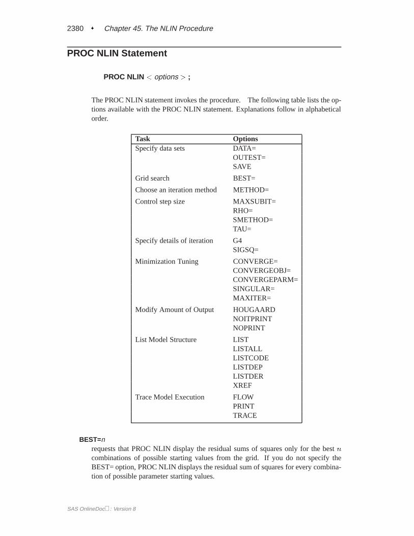
PROC NLIN Statement

PROC NLIN < options > ;

The PROC NLIN statement invokes the procedure. The following table lists the op-tions available with the PROC NLIN statement. Explanations follow in alphabeticalorder.

Task OptionsSpecify data sets DATA=

OUTEST=SAVE

Grid search BEST=

Choose an iteration method METHOD=

Control step size MAXSUBIT=RHO=SMETHOD=TAU=

Specify details of iteration G4SIGSQ=

Minimization Tuning CONVERGE=CONVERGEOBJ=CONVERGEPARM=SINGULAR=MAXITER=

Modify Amount of Output HOUGAARDNOITPRINTNOPRINT

List Model Structure LISTLISTALLLISTCODELISTDEPLISTDERXREF

Trace Model Execution FLOWPRINTTRACE

BEST=nrequests that PROC NLIN display the residual sums of squares only for the bestncombinations of possible starting values from the grid. If you do not specify theBEST= option, PROC NLIN displays the residual sum of squares for every combina-tion of possible parameter starting values.


PROC NLIN Statement � 2381

CONVERGE=cspecifies the convergence criteria for PROC NLIN. For all iterative methods exceptfor METHOD=DUD, the relative offset convergence measure of Bates and Wattsis used to determine convergence. This measure is labeled "R" in the EstimationSummary table. The iterations are said to have converged for CONVERGE=c if

rr0X(X 0X)�1X 0r

LOSSi< c

wherer is the residual vector andX is the Jacobian matrix. The default LOSS func-tion is the sum of squared errors (SSE). By default, CONVERGE=10�5. The Rconvergence measure cannot be computed accurately in the special case of a perfectfit ( residuals close to zero). When the SSE is less than the value of the SINGULAR=option, convergence is assumed.

CONVERGEOBJ=c (DUD only)uses the change in the LOSS function as the convergence criterion. For more de-tails on the LOSS function, see the section “Special Variable Used to DetermineConvergence Criteria” on page 2396. The iterations are said to have converged forCONVERGEOBJ=c if

LOSSi�1 � LOSSi

LOSSi + 10�6< c

where LOSSi is the LOSS for theith iteration. The default LOSS function is thesum of squared errors (SSE). The constantc should be a small positive number. Seethe “Computational Methods” section beginning on page 2398 for more details. Bydefault, CONVERGE=10�8.

CONVERGEPARM=c (DUD only)uses the maximum change among parameter estimates as the convergence criterion.The iterations are said to have converged for CONVERGEPARM=c if

maxj

j�i�1j � �ij jj�i�1j j

!< c

where�ij is the value of thejth parameter at theith iteration.

The default convergence criterion for DUD is CONVERGEOBJ. If you specifyCONVERGEOBJ=c, the specifiedc is used instead of the default of10�8. If youspecify CONVERGEPARM=c, the maximum change in parameters is used as theconvergence criterion (instead of LOSS). If you specify both the CONVERGEOBJ=and CONVERGEPARM= options, PROC NLIN continues to iterate until the de-crease in LOSS is sufficiently small (as determined by the CONVERGEOBJ= option)and the maximum change among the parameters is sufficiently small (as determinedby the CONVERGEPARM= option).

DATA=SAS-data-setspecifies the SAS data set containing the data to be analyzed by PROC NLIN. If youomit the DATA= option, the most recently created SAS data set is used.



FLOWdisplays a message for each statement in the model program as it is executed. Thisdebugging option is rarely needed, and it produces large amounts of output.

G4uses a Moore-Penrose (g4) inverse in parameter estimation. Refer to Kennedy andGentle (1980) for details.

HOUGAARDadds Hougaard’s measure of skewness to the parameter estimation table. Compu-tation of the measure requires derivatives (see the section “Hougaard’s Measure ofSkewness” on page 2394). Thus, the HOUGAARD option is ignored if you specifythe option METHOD=DUD, which is described later in this list.

LISTdisplays the model program and variable lists, including the statements added bymacros. Note that the expressions displayed by the LIST option do not necessarilyrepresent the way the expression is actually calculated, since intermediate results forcommon subexpressions can be reused but are shown in expanded form by the LISToption. To see how the expression is actually evaluated, see the description for theLISTCODE option, which follows.

LISTALLselects the LIST, LISTDEP, LISTDER, and LISTCODE options.

LISTCODEdisplays the derivative tables and compiled model program code. The LISTCODEoption is a debugging feature and is not normally needed.

LISTDEPproduces a report that lists, for each variable in the model program, the variables thatdepend on it and on which it depends.

LISTDERdisplays a table of derivatives. The derivatives table lists each nonzero derivativecomputed for the problem. The derivative listed can be a constant, a variable inthe model program, or a special derivative variable created to hold the result of thederivative expression.

MAXITER=ilimits the number of iterations PROC NLIN performs before it gives up trying toconverge. Thei value must be a positive integer. By default, MAXITER=100.

MAXSUBIT= iplaces a limit on the number of step halvings. By default, MAXSUBIT=30. Thevalue of MAXSUBIT must be a positive integer.

METHOD=GAUSS | MARQUARDT | NEWTON | GRADIENT | DUDspecifies the iterative method that PROC NLIN uses. The GAUSS, MARQUARDTand NEWTON methods are more robust than the GRADIENT and DUD methods.If you omit the METHOD= option, METHOD=GAUSS is used. See the “Computa-tional Methods” section beginning on page 2398 for more information.


PROC NLIN Statement � 2383

NOITPRINTsuppresses the display of the results of each iteration.

NOPRINTsuppresses the display of the output. Note that this option temporarily disables theOutput Delivery System (ODS). For more information, see Chapter 15, “Using theOutput Delivery System.”

OUTEST=SAS datasetspecifies an output data set to contain the parameter estimates produced at each it-eration. See the “Output Data Sets” section on page 2403 for details. If you wantto create a permanent SAS data set, you must specify a two-level name. See thechapter “SAS Files,” inSAS Language Reference: Conceptsfor more information onpermanent SAS data sets.

PRINTdisplays the result of each statement in the program as it is executed. This optionproduces large amounts of output.

RHO=valuespecifies a value to use in controlling the step-size search. By default, RHO=0.1except when METHOD=MARQUARDT, in which case RHO=10. See the section“Computational Methods” beginning on page 2398 for more details.

SAVEspecifies that, when the iteration limit is exceeded, the parameter estimates from thefinal iteration are output to the OUTEST= data set. These parameter estimates arelocated in the observation with–TYPE–=FINAL. If you omit the SAVE option,the parameter estimates from the final iteration are not output to the data set unlessconvergence is attained.

SIGSQ=valuespecifies a value to replace the mean square error for computing the standard errorsof the estimates. The SIGSQ= option is used with maximum-likelihood estimation.

SINGULAR=sspecifies the singularity criterion,s, which is the absolute magnitude of the smallestpivot value allowed when inverting the Hessian or approximation to the Hessian. Thedefault value is 1E-8.

SMETHOD=HALVE | GOLDEN | CUBICspecifies the step-size search method that PROC NLIN uses. The default isSMETHOD=HALVE. See the section “Computational Methods” beginning onpage 2398 for details.

TAU=valuespecifies a value to use in controlling the step-size search. By default, TAU=1 ex-cept when METHOD=MARQUARDT, in which case TAU=0.01. See the section“Computational Methods” beginning on page 2398 for details.



TRACEdisplays the result of each operation in each statement in the model program as it isexecuted, in addition to the information displayed by the FLOW and PRINT options.This debugging option is needed very rarely, and it produces even more output thanthe FLOW and PRINT options.

XREFdisplays a cross-reference of the variables in the model program showing where eachvariable is referenced or given a value. The XREF listing does not include derivativevariables.

BOUNDS Statement

BOUNDS inequality <; : : : ; inequality > ;

The BOUNDS statement restrains the parameter estimates within specified bounds.In each BOUNDS statement, you can specify a series of bounds separated by com-mas. The series of bounds is applied simultaneously. Each bound contains a listof parameters, an inequality comparison operator, and a value. In a single-boundedexpression, these three elements follow one another in the order described. The fol-lowing are examples of valid single-bounded expressions:

bounds a1-a10<=20;bounds c>30;bounds a b c > 0;

Multiple-bounded expressions are also permitted. For example,

bounds 0<=B<=10;bounds 15<x1<=30;bounds r <= s <= p < q;

If you need to restrict an expression involving several parameters (for example,A + B < 1), you can reparameterize the model so that the expression becomes aparameter.

For SAS versions 7.01 and later, lagrange multipliers are reported for all bounds thatare enforced (active) when the estimation terminates. In the estimates table and inthe OUTEST= data set, the Lagrange multiplier estimates are identified with namesBound1, Bound2... . An active bound is treated as if a restriction was applied tothe set of parameters so one parameter degree of freedom is deducted. The optionNOCORRECTEDDF specifies that no degrees of freedom are lost when a bound isactive. Lagrange multiplier based bounds are not used for METHOD=DUD.


DER Statements � 2385

BY Statement

BY variables ;

You can specify a BY statement with PROC NLIN to obtain separate analyses onobservations in groups defined by the BY variables. When a BY statement appears,the procedure expects the input data set to be sorted in order of the BY variables.

If your input data set is not sorted in ascending order, use one of the following alter-natives:

� Sort the data using the SORT procedure with a similar BY statement.

� Specify the BY statement option NOTSORTED or DESCENDING in the BYstatement for the NLIN procedure. The NOTSORTED option does not meanthat the data are unsorted but rather that the data are arranged in groups (ac-cording to values of the BY variables) and that these groups are not necessarilyin alphabetical or increasing numeric order.

� Create an index on the BY variables using the DATASETS procedure.

For more information on the BY statement, refer to the discussion inSAS LanguageReference: Concepts. For more information on the DATASETS procedure, refer tothe discussion in theSAS Procedures Guide.

CONTROL Statement

CONTROLvariable <=values> < : : : variable <=values>> ;

The CONTROL statement declares control variables and specifies their values. Acontrol variable is like a retained variable (see the section “RETAIN Statement” onpage 2390) except that it is retainedacrossiterations and the derivative of the modelwith respect to a control variable is always zero.

DER Statements

DER.parameter=expression ;DER.parameter.parameter=expression ;

The DER statement specifies first or second partial derivatives. By default, analyticalderivatives are automatically computed. However, you can specify the derivativesyourself by using the DER.parm syntax. Use the first form shown to specify firstpartial derivatives, and use the second form to specify second partial derivatives. Notethat the DER.parm syntax is retained for backward compatibility. The automaticanalytical derivatives are, in general, a better choice. For additional information on



automatic analytical derivatives, see the section “Automatic Derivatives” beginningon page 2391.

For most of the computational methods, you need only specify the first partial deriva-tive for each parameter to be estimated. For the NEWTON method, specify both thefirst and the second derivatives. If any needed derivatives are not specified, they areautomatically computed.

If you use the–LOSS– variable, you can specify the derivative of–LOSS– with re-spect to the parameters using the DER. syntax.For more information, see the “SpecialVariable Used to Determine Convergence Criteria” section on page 2396.

The expression can be an algebraic representation of the partial derivative of the ex-pression in the MODEL statement with respect to the parameter or parameters thatappear in the left-hand side of the DER statement. Numerical derivatives can also beused. The expression in the DER statement must conform to the rules for a valid SASexpression, and it can include any quantities that the MODEL statement expressioncontains.

ID Statement

ID variables ;

The ID statement specifies additional variables to place in the output data set createdby the OUTPUT statement. Any variable on the left-hand side of any assignmentstatement is eligible. Also, the special variables created by the procedure can bespecified. Variables in the input data set do not need to be specified in the ID state-ment since they are automatically included in the output data set.

MODEL Statement

MODEL dependent=expression ;

The MODEL statement defines the prediction equation by declaring the dependentvariable and defining an expression that evaluates predicted values. The expressioncan be any valid SAS expression yielding a numeric result. The expression can in-clude parameter names, variables in the data set, and variables created by programstatements in the NLIN procedure. Any operators or functions that can be used in aDATA step can also be used in the MODEL statement.

A statement such as

model y= expression;

is translated into the form

model.y= expression;


OUTPUT Statement � 2387

using the compound variable namemodel.y to hold the predicted value. You canuse this assignment as an alternative to the MODEL statement. Either a MODELstatement or an assignment to a compound variable such asmodel.y must appear.

OUTPUT Statement

OUTPUT OUT=SAS-data-set keyword=names <; : : : ;keyword=names>;

The OUTPUT statement specifies an output data set to contain statistics calculatedfor each observation. For each statistic, specify the keyword, an equal sign, and avariable name for the statistic in the output data set. All of the names appearing in theOUTPUT statement must be valid SAS names, and none of the new variable namescan match a variable already existing in the data set to which PROC NLIN is applied.

If an observation includes a missing value for one of the independent variables, boththe predicted value and the residual value are missing for that observation. If theiterations fail to converge, all the values of all the variables named in the OUTPUTstatement are missing values.

You can specify the following options in the OUTPUT statement. For a descriptionof computational formulas, see Chapter 3, “Introduction to Regression Procedures.”

OUT=SAS data setspecifies the SAS data set to be created by PROC NLIN when an OUTPUT statementis included. The new data set includes all the variables in the data set to which PROCNLIN is applied. Also included are any ID variables specified in the ID statement,plus new variables with names that are specified in the OUTPUT statement.

The following values can be calculated and output to the new data set. However, withMETHOD=DUD, the following statistics are not available: H, L95, L95M, STDP,STDR, STUDENT, U95, and U95M. These statistics are all calculated using H, thevariable containing the leverage. For METHOD=DUD, the approximate Hessian isnot available since no derivatives are specified with this method.

H=namespecifies a variable to contain the leverage,xi(X

0X)�1x0i, whereX = @F=@� and

xi is theith row ofX. If you specify the special variable–WEIGHT– , the leverageiswixi(X

0WX)�1x0i.

L95M=namespecifies a variable to contain the lower bound of an approximate 95% confidence in-terval for the expected value (mean). See also the description for the U95M= option,which follows.

L95=namespecifies a variable to contain the lower bound of an approximate 95% confidenceinterval for an individual prediction. This includes the variance of the error as well asthe variance of the parameter estimates. See also the description for the U95= option,which follows.



PARMS=namesspecifies variables in the output data set to contain parameter estimates. These can bethe same variable names as listed in the PARAMETERS statement; however, you canchoose new names for the parameters identified in the sequence from the PARAME-TERS statement. Note that, for each of these new variables, the values are the samefor every observation in the new data set.

PREDICTED=nameP=name

specifies a variable in the output data set to contain the predicted values of the depen-dent variable.

RESIDUAL=nameR=name

specifies a variable in the output data set to contain the residuals (actual values minuspredicted values).

SSE=nameESS=name

specifies a variable to include in the new data set. The values for the variable arethe residual sums of squares finally determined by the procedure. The values of thevariable are the same for every observation in the new data set.

STDI=namespecifies a variable to contain the standard error of the individual predicted value.

STDP=namespecifies a variable to contain the standard error of the mean predicted value.

STDR=namespecifies a variable to contain the standard error of the residual.

STUDENT=namespecifies a variable to contain the studentized residuals, which are residuals dividedby their standard errors.

U95M=namespecifies a variable to contain the upper bound of an approximate 95% confidenceinterval for the expected value (mean). See also the description for the L95M= option.

U95=namespecifies a variable to contain the upper bound of an approximate 95% confidenceinterval for an individual prediction. See also the description for the L95= option.

WEIGHT=namespecifies a variable in the output data set that contains values of the special variable

–WEIGHT– .


PARAMETERS Statement � 2389

PARAMETERS Statement

PARAMETERS parameter=values : : : ;PARMS parameter=values : : : ;

A PARAMETERS (or PARMS) statement must come before the RUN statement.Several parameter names and values can appear. The parameter names must all bevalid SAS names and must not duplicate the names of any variables in the data set towhich the NLIN procedure is applied. Any parameters specified but not used in theMODEL statement are dropped from the estimation.

In eachparameter=valuesspecification, the parameter name identifies a parameterto be estimated, both in subsequent procedure statements and in the output.Valuesspecify the possible starting values of the parameter.

Usually, only one value is specified for each parameter. If you specify several valuesfor each parameter, PROC NLIN evaluates the model at each point on the grid. Thevalue specifications can take any of several forms:

m a single value

m1,m2, : : : , mn several values

m TO n a sequence wherem equals the starting value,n equals the endingvalue, and the increment equals 1

m TO n BY i a sequence wherem equals the starting value,n equals the endingvalue, and the increment isi

m1,m2 TOm3 mixed values and sequences

This PARMS statement specifies five parameters and sets their possible starting val-ues as shown:

parms b0=0b1=4 to 8b2=0 to .6 by .2b3=1, 10, 100b4=0, .5, 1 to 4;

Possible starting valuesB0 B1 B2 B3 B4

0 4 0.0 1 0.05 0.2 10 0.56 0.4 100 1.07 0.6 2.08 3.0

4.0



Residual sums of squares are calculated for each of the1�5�4�3�6 = 360 com-binations of possible starting values. (This can take a long time.) See the “SpecialVariables” section beginning on page 2395 for information on programming param-eter starting values.

RETAIN Statement

RETAIN variable <=values> < : : : variable <=values>> ;

The RETAIN statement declares retained variables and specifies their values. A re-tained variable is like a control variable (see the section “CONTROL Statement” onpage 2385) except that it is retained onlywithin iterations. An iteration involves asingle pass through the data set.

Other Program Statements with PROC NLIN

PROC NLIN supports many statements that are similar to SAS programming state-ments used in a DATA step. However, there are some differences in capabilities;for additional information, see the section “Incompatibilities with 6.11 and EarlierVersions of PROC NLIN” beginning on page 2406.

Several SAS program statements can be used after the PROC NLIN statement. Thesestatements can appear anywhere in the PROC NLIN statement, but new variablesmust be created before they appear in other statements. For example, the followingstatements are valid since they create the variabletemp before they use it in theMODEL statement:

proc nlin;parms b0=0 to 2 by 0.5 b1=0.01 to 0.09 by 0.01;temp=exp(-b1*x);model y=b0*(1-temp);

The following statements result in missing values fory because the variabletemp isundefined before it is used:

proc nlin;parms b0=0 to 2 by 0.5 b1=0.01 to 0.09 by 0.01;model y=b0*(1-temp);temp=exp(-b1*x);

PROC NLIN can process assignment statements, explicitly or implicitly subscriptedARRAY statements, explicitly or implicitly subscripted array references, IF state-ments, SAS functions, and program control statements. You can use program state-ments to create new SAS variables for the duration of the procedure. These vari-ables are not permanently included in the data set to which PROC NLIN is applied.Program statements can include variables in the DATA= data set, parameter names,variables created by preceding program statements within PROC NLIN, and special


Automatic Derivatives � 2391

variables used by PROC NLIN. All of the following SAS program statements can beused in PROC NLIN:

� ARRAY

� assignment (y = a*x + b; )

� CALL

� DO

� iterative DO

� DO UNTIL

� DO WHILE

� END

� FILE

� GO TO

� IF-THEN/ELSE

� LINK-RETURN

� PUT (defaults to the list)

� RETURN

� SELECT

� sum (y + 1; )

These statements can use the special variables created by PROC NLIN. Consult thesection “Special Variables” beginning on page 2395 for more information on specialvariables.

Details

Automatic Derivatives

Depending on the optimization method you select, analytical first- and second-orderderivatives are computed automatically. Derivatives can still be supplied using theDER.parm syntax. These DER.parm derivatives are not verified by the differentia-tor. If any needed derivatives are not supplied, they are computed and added to theprogram statements. To view the computed derivatives, use the LISTDER or LISToption.

The following model is solved using Newton’s method. Analytical first- and second-order derivatives are automatically computed.



proc nlin data=Enzyme method=newton list;parms x1=4 x2=2 ;model Velocity = x1 * exp (x2 * Concentration);

run;

The NLIN Procedure

Listing of Compiled Program CodeStmt Line:Col Statement as Parsed

1 471:74 MODEL.Velocity = x1 * EXP(x2* Concentration);

1 471:74 @MODEL.Velocity/@x1 = EXP(x2* Concentration);

1 471:74 @MODEL.Velocity/@x2 = x1 * Concentration* EXP(x2 * Concentration);

1 471:74 @@MODEL.Velocity/@x1/@x2 = Concentration* EXP(x2 * Concentration);

1 471:74 @@MODEL.Velocity/@x2/@x1 = Concentration* EXP(x2 * Concentration);

1 471:74 @@MODEL.Velocity/@x2/@x2 = x1* Concentration * Concentration* EXP(x2 * Concentration);

Figure 45.5. Model and Derivative Code Output

Note that all the derivatives require the evaluation of EXP(X2 *Concentration). Ifyou specify the LISTCODE option in the PROC NLIN statement, the actual machinelevel code produced is as follows.


Automatic Derivatives � 2393

The NLIN Procedure

Code Listing

1 Stmt MODEL line 328 column 78.(1)arg=MODEL.Velocityargsave=MODEL.VelocitySource Text: model Velocity = x1 * exp

(x2 * Concentration);Oper * at 328:108 (30,0,2). * : #temp1 <- x2 ConcentrationOper EXP at 328:104 EXP : #temp2 <- #temp1

(103,0,1).Oper * at 328:98 (30,0,2). * : MODEL.Velocity <- x1 #temp2Oper eeocf at 328:104 (18,0,1). eeocf : _DER_ <- _DER_Oper * at 328:104 (30,0,2). * : @1dt1_1 <- Concentration #temp2Oper = at 328:98 (1,0,1). = : @MODEL.Velocity/@x1 <- #temp2Oper * at 328:98 (30,0,2). * : @MODEL.Velocity/@x2

<- x1 @1dt1_1Oper * at 328:104 (30,0,2). * : @2dt1_1 <- Concentration

@1dt1_1Oper = at 328:98 (1,0,1). = : @@MODEL.Velocity/@x1/@x2

<- @1dt1_1Oper = at 328:98 (1,0,1). = : @@MODEL.Velocity/@x2/@x1

<- @1dt1_1Oper * at 328:98 (30,0,2). * : @@MODEL.Velocity/@x2/@x2

<- x1 @2dt1_1

Figure 45.6. LISTCODE Output

Note that, in the generated code, only one exponentiation is performed. The generatedcode reuses previous operations to be more efficient.



Hougaard’s Measure of Skewness

A “close-to-linear” nonlinear regression model, first described by Ratkowsky (1990),is a model that produces parameters having properties similar to those produced bya linear regression model. That is, the least squares estimates of the parameters areclose to being unbiased, normally distributed, minimum variance estimators.

A nonlinear regression model sometimes fails to be close to linear due to the prop-erties of a single parameter. When this occurs, bias in the parameters can renderinferences using the reported standard errors and confidence limits invalid. You canoften fix the problem with reparameterization, replacing the offending parameter byone with better estimation properties.

You can use Hougaard’s measure of skewness,g1i, to assess whether a parame-ter is close to linear or whether it contains considerable nonlinearity. Specify theHOUGAARD option in the PROC NLIN statement to compute Hougaard’s measureof skewness.

According to Ratkowsky (1990), ifjg1ij < 0:1, the estimator�i of parameter�i isvery close-to-linear in behavior and, if0:1 < jg1ij < :25, the estimator is reasonablyclose-to-linear. Ifjg1ij > :25, the skewness is very apparent. Forjg1ij > 1, thenonlinear behavior is considerable.

Hougaard’s measure is computed as follows

E[�i �E(�i)]3 = �(mse)2

npXjkl

LijLikLil(Wjkl +Wkjl +Wlkj)

where the sum is a triple sum over the number of parameters and

L = X 0X�1

Wjkl =

nXm=1

J jmHklm

In the preceding equation,Jm is the Jacobian vector andHm is the Hessian matrixevaluated at observationm. This third moment is normalized using the standard erroras

g1i = E[�i �E(�i)]3=(mse � Lii)3=2

Missing Values

If the value of any one of the SAS variables involved in the model is missing froman observation, that observation is omitted from the analysis. If only the value of thedependent variable is missing, that observation has a predicted value calculated for itwhen you use an OUTPUT statement and specify the PREDICTED= option.


Special Variables � 2395

If an observation includes a missing value for one of the independent variables, boththe predicted value and the residual value are missing for that observation. If theiterations fail to converge, all the values of all the variables named in the OUTPUTstatement are missing values.

Special Variables

Several special variables are created automatically and can be used in PROC NLINprogram statements.

Special Variables with Values that are Set by PROC NLINThe values of the following six special variables are set by PROC NLIN and shouldnot be reset to a different value by programming statements:

–ERROR– is set to 1 if a numerical error or invalid argument to a functionoccurs during the current execution of the program. It is reset to 0before each new execution.

–ITER– represents the current iteration number. The variable–ITER– isset to�1 during the grid search phase.

–MODEL– is set to 1 for passes through the data when only the predicted val-ues are needed, not the derivatives. It is 0 when both predictedvalues and derivatives are needed. If your derivative calculationsconsume a lot of time, you can save resources by coding

if _model_ then return;

after your MODEL statement but before your derivative calcula-tions. The derivatives generated by PROC NLIN do this automati-cally.

–N– indicates the number of times the PROC NLIN step has been exe-cuted. It is never reset for successive passes through the data set.

–OBS– indicates the observation number in the data set for the current pro-gram execution. It is reset to 1 to start each pass through the dataset (unlike the–N– variable).

–SSE– has the error sum of squares of the last iteration. During the gridsearch phase, the–SSE– variable is set to 0. For iteration 0, the

–SSE– variable is set to the SSE associated with the point chosenfrom the grid search.



Special Variable Used to Determine Convergence CriteriaThe special variable–LOSS– can be used to determine convergence criteria:

–LOSS– is used to determine the criterion function for convergence and stepshortening. PROC NLIN looks for the variable–LOSS– in theprogram statements and, if it is defined, uses the (weighted) sumof this value instead of the residual sum of squares to determinethe criterion function for convergence and step shortening. Thisfeature is useful in certain types of maximum-likelihood estimationwhere the residual sum of squares is not the basic criterion.

Weighted Regression with the Special Variable –WEIGHT–To get weighted least squares estimates of parameters, the–WEIGHT– variable canbe given a value in an assignment statement:

_weight_ = expression ;

When this statement is included, the expression on the right-hand side of the assign-ment statement is evaluated for each observation in the data set to be analyzed. Thevalues obtained are taken as inverse elements of the diagonal variance-covariancematrix of the dependent variable.

When a variable name is given after the equal sign, the values of the variable aretaken as the inverse elements of the variance-covariance matrix. The larger the

–WEIGHT– value, the more importance the observation is given.

If the –WEIGHT–= statement is not used, the default value of 1 is used, and regularleast squares estimates are obtained.

Troubleshooting

This section describes a number of problems that can occur in your analysis withPROC NLIN.

Excessive TimeIf you specify a grid of starting values that contains many points, the analysis maytake excessive time since the procedure must go through the entire data set for eachpoint on the grid.

The analysis may also take excessive time if your problem takes many iterationsto converge since each iteration requires as much time as a linear regression withpredicted values and residuals calculated.

DependenciesThe matrix of partial derivatives may be singular, possibly indicating an over-parameterized model. For example, ifb0 starts at zero in the following model, thederivatives forb1 are all zero for the first iteration.


Troubleshooting � 2397

parms b0=0 b1=.022;model pop=b0*exp(b1*(year-1790));der.b0=exp(b1*(year-1790));der.b1=(year-1790)*b0*exp(b1*(year-1790));

The first iteration changes a subset of the parameters; then the procedure can makeprogress in succeeding iterations. This singularity problem is local. The next exampledisplays a global problem.

You may have a termb2 in the exponent that is nonidentifiable since it trades roleswith b0.

parms b0=3.9 b1=.022 b2=0;model pop=b0*exp(b1*(year-1790)+b2);der.b0=exp(b1*(year-1790)+b2);der.b1=(year-1790)*b0*exp(b1*(year-1790)+b2);der.b2=b0*exp(b1*(year-1790)+b2);

Unable to ImproveThe method may lead to steps that do not improve the estimates even after a series ofstep halvings. If this happens, the procedure issues a message stating that it is unableto make further progress, but it then displays the warning message

PROC NLIN failed to converge

and displays the results. This often means that the procedure has not converged atall. If you provided the derivatives, check them very closely and then check the sum-of-squares error surface before proceeding. If PROC NLIN has not converged, try adifferent set of starting values, a different METHOD= specification, the G4 option,or a different model.

DivergenceThe iterative process may diverge, resulting in overflows in computations. It is alsopossible that parameters enter a space where arguments to such functions as LOG andSQRT become illegal. For example, consider the following model:

parms b=0;model y=x / b;

Suppose thaty happens to be all zero andx is nonzero. There is no least squaresestimate forb since the SSE declines asb approaches infinity or minus infinity. Thesame model could be parameterized with no problem intoy = a*x.

If you have divergence problems, try reparameterizing, selecting different startingvalues, increasing the maximum allowed number of iterations (the MAXITER= op-tion), specifying an alternative METHOD= option, or including a BOUNDS state-ment.

Local MinimumThe program may converge to a local rather than a global minimum. For example,consider the following model.



parms a=1 b=-1;model y=(1-a*x)*(1-b*x);

Once a solution is found, an equivalent solution with the same SSE can be obtainedby swapping the values ofa andb.

DiscontinuitiesThe computational methods assume that the model is a continuous and smooth func-tion of the parameters. If this is not true, the method does not work. For example, thefollowing models do not work:

model y=a+int(b*x);

model y=a+b*x+4*(z>c);

Responding to TroublePROC NLIN does not necessarily produce a good solution the first time. Much de-pends on specifying good initial values for the parameters. You can specify a gridof values in the PARMS statement to search for good starting values. While mostpractical models should give you no trouble, other models may require switching toa different iteration method or an inverse computation method. Specifying the op-tion METHOD=MARQUARDT sometimes works when the default method (Gauss-Newton) does not work.

Computational Methods

For the system of equations represented by the nonlinear model

Y = F(�0; �1; : : : ; �r;Z1;Z2; : : : ;Zn) + � = F(��) + �

whereZ is a matrix of the independent variables,�� is a vector of the parameters,� isthe error vector, andF is a function of the independent variables and the parameters,there are two approaches to solving for the minimum. The first method is to minimize

L(�) = 0:5(e0e)

wheree = Y � F(�) and� is an estimate of��.

The second method is to solve the nonlinear “normal” equations

X0F(�) = X0

Y

where

X =@F

@�

In the nonlinear situation, bothX andF(�) are functions of� and a closed-formsolution generally does not exist. Thus, PROC NLIN uses an iterative process: a


Computational Methods � 2399

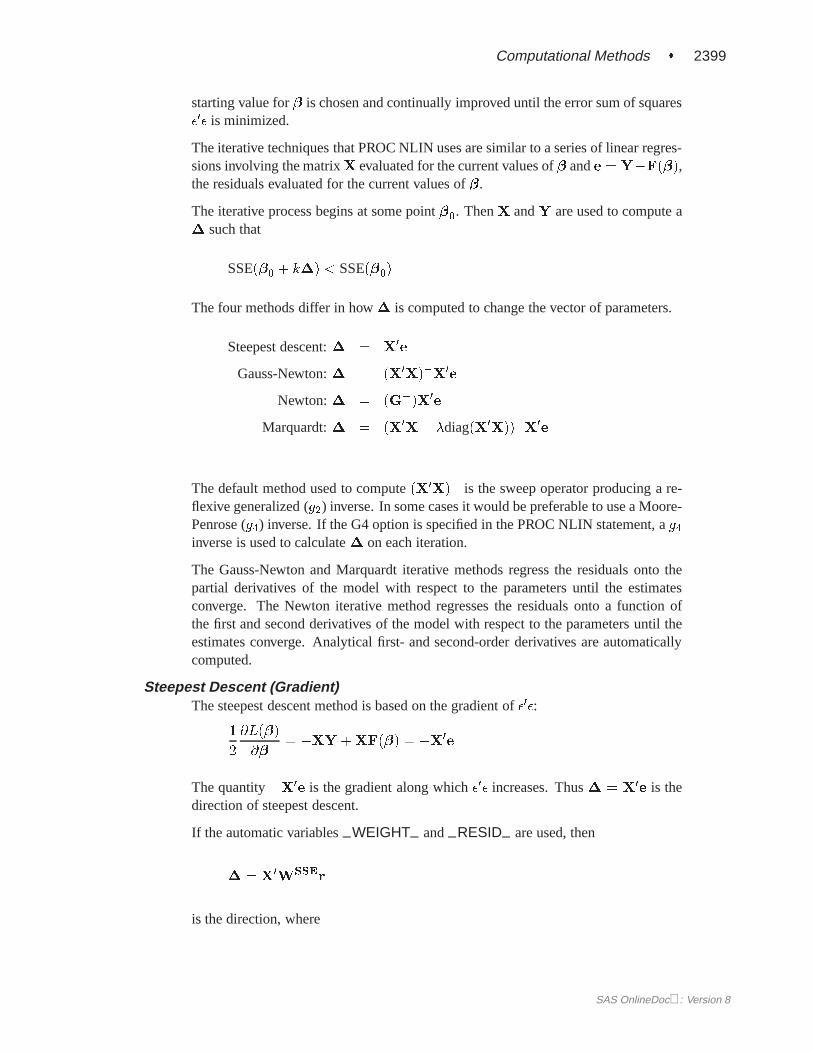
starting value for� is chosen and continually improved until the error sum of squares�0� is minimized.

The iterative techniques that PROC NLIN uses are similar to a series of linear regres-sions involving the matrixX evaluated for the current values of� ande = Y�F(�),the residuals evaluated for the current values of�.

The iterative process begins at some point�0. ThenX andY are used to compute a� such that

SSE(�0 + k�) < SSE(�0)

The four methods differ in how� is computed to change the vector of parameters.

Steepest descent:� = X0e

Gauss-Newton:� = (X0X)�X0

e

Newton:� = (G�)X0e

Marquardt:� = (X0X+ �diag(X0

X))�X0e

The default method used to compute(X0X)� is the sweep operator producing a re-

flexive generalized (g2) inverse. In some cases it would be preferable to use a Moore-Penrose (g4) inverse. If the G4 option is specified in the PROC NLIN statement, ag4inverse is used to calculate� on each iteration.

The Gauss-Newton and Marquardt iterative methods regress the residuals onto thepartial derivatives of the model with respect to the parameters until the estimatesconverge. The Newton iterative method regresses the residuals onto a function ofthe first and second derivatives of the model with respect to the parameters until theestimates converge. Analytical first- and second-order derivatives are automaticallycomputed.

Steepest Descent (Gradient)The steepest descent method is based on the gradient of�0�:

1

2

@L(�)

@�= �XY +XF(�) = �X0

e

The quantity�X0e is the gradient along which�0� increases. Thus� = X

0e is the

direction of steepest descent.

If the automatic variables–WEIGHT– and–RESID– are used, then

� = X0W

SSEr

is the direction, where



WSSE is an n � n diagonal matrix with elementswSSE

i of weights fromthe –WEIGHT– variable. Each elementwSSE

i contains the value of

–WEIGHT– for theith observation.

r is a vector with elementsri from –RESID– . Each elementri contains thevalue of–RESID– evaluated for theith observation.

Using the method of steepest descent, let

�k+1 = �k + ��

where the scalar� is chosen such that

SSE(�i + ��) < SSE(�i)

Note: The steepest descent method may converge very slowly and is therefore notgenerally recommended. It is sometimes useful when the initial values are poor.

NewtonThe Newton method uses the second derivatives and solves the equation

� = G�X0e

where

G = (X0X) +

nXi=1

Hi(�)ei

andHi(�) is the Hessian ofe:

[Hi]jk =

�@2ei

@�j@�k

�jk

If the automatic variables–WEIGHT– , –WGTJPJ–, and–RESID– are used, then

� = G�X0W

SSEr

is the direction, where

G = X0W

XPXX+

nXi=1

Hi(�)wXPXi ri

and

WSSE is an n � n diagonal matrix with elementswSSE

i of weights fromthe –WEIGHT– variable. Each elementwSSE

i contains the value of

–WEIGHT– for theith observation.


Computational Methods � 2401

WXPX is ann � n diagonal matrix with elementswXPX

i of weights from the

–WGTJPJ– variable.

Each elementwXPXi contains the value of–WGTJPJ– for theith observa-

tion.

r is a vector with elementsri from the–RESID– variable. Each elementricontains the value of–RESID– evaluated for theith observation.

Gauss-NewtonThe Gauss-Newton method uses the Taylor series

F(�) = F(�0) +X(� � �0) + � � �

whereX = @F=@� is evaluated at� = �0.

Substituting the first two terms of this series into the normal equations

X0F(�) = X

0Y

X0(F(�0) +X(� � �0)) = X

0Y

(X0X)(� � �0) = X

0Y �X0

F(�0)

(X0X)� = X

0e

and therefore

� = (X0X)�X0

e

Caution: IfX0X is singular or becomes singular, PROC NLIN computes� using a

generalized inverse for the iterations after singularity occurs. IfX0X is still singular

for the last iteration, the solution should be examined.

MarquardtThe Marquardt updating formula is as follows:

� = (X0X+ �diag(X0

X))�X0e

The Marquardt method is a compromise between the Gauss-Newton and steepestdescent methods (Marquardt 1963). As� ! 0, the direction approaches Gauss-Newton. As�!1, the direction approaches steepest descent.

Marquardt’s studies indicate that the average angle between Gauss-Newton and steep-est descent directions is about90�. A choice of� between 0 and infinity produces acompromise direction.

By default, PROC NLIN chooses� = 10�3 to start and computes a�. If SSE(�0 +�) < SSE(�0), then� = �=10 for the next iteration. Each time SSE(�0 +�) >SSE(�0), then� = 10�.



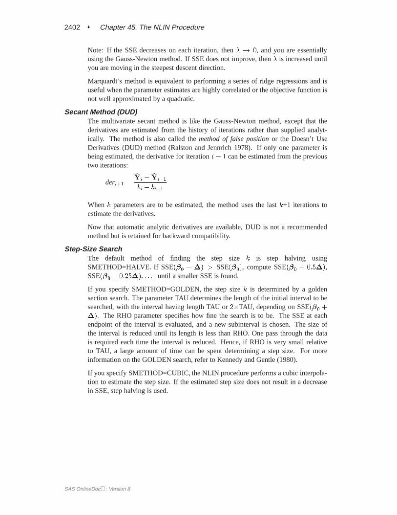
Note: If the SSE decreases on each iteration, then� ! 0, and you are essentiallyusing the Gauss-Newton method. If SSE does not improve, then� is increased untilyou are moving in the steepest descent direction.

Marquardt’s method is equivalent to performing a series of ridge regressions and isuseful when the parameter estimates are highly correlated or the objective function isnot well approximated by a quadratic.

Secant Method (DUD)The multivariate secant method is like the Gauss-Newton method, except that thederivatives are estimated from the history of iterations rather than supplied analyt-ically. The method is also called themethod of false positionor the Doesn’t UseDerivatives (DUD) method (Ralston and Jennrich 1978). If only one parameter isbeing estimated, the derivative for iterationi+ 1 can be estimated from the previoustwo iterations:

deri+1 =Yi � Yi�1

bi � bi�1

Whenk parameters are to be estimated, the method uses the lastk+1 iterations toestimate the derivatives.

Now that automatic analytic derivatives are available, DUD is not a recommendedmethod but is retained for backward compatibility.

Step-Size SearchThe default method of finding the step sizek is step halving usingSMETHOD=HALVE. If SSE(�0 + �) > SSE(�0), compute SSE(�0 + 0:5�),SSE(�0 + 0:25�); : : : ; until a smaller SSE is found.

If you specify SMETHOD=GOLDEN, the step sizek is determined by a goldensection search. The parameter TAU determines the length of the initial interval to besearched, with the interval having length TAU or2�TAU, depending on SSE(�0 +�). The RHO parameter specifies how fine the search is to be. The SSE at eachendpoint of the interval is evaluated, and a new subinterval is chosen. The size ofthe interval is reduced until its length is less than RHO. One pass through the datais required each time the interval is reduced. Hence, if RHO is very small relativeto TAU, a large amount of time can be spent determining a step size. For moreinformation on the GOLDEN search, refer to Kennedy and Gentle (1980).

If you specify SMETHOD=CUBIC, the NLIN procedure performs a cubic interpola-tion to estimate the step size. If the estimated step size does not result in a decreasein SSE, step halving is used.


Confidence Intervals � 2403

Output Data Sets

The data set produced by the OUTEST= option in the PROC NLIN statement containsthe parameter estimates on each iteration including the grid search.

The variable–ITER– contains the iteration number. The variable–TYPE– denoteswhether the observation contains iteration parameter estimates (’ITER’), final param-eter estimates (’FINAL’), or covariance estimates (’COVB’). The variable–NAME–contains the parameter name for covariances, and the variable–SSE– contains theobjective function value for the parameter estimates. The variable–STATUS– indi-cates whether the estimates have converged.

The data set produced by the OUTPUT statement contains statistics calculated foreach observation. In addition, the data set contains all the variables in the input dataset and any ID variables that are specified in the ID statement.

Confidence Intervals

Parameter Confidence IntervalsThe parameter confidence intervals are computed using the Wald based formula:

�i � stderri � t(N � P; 0:05=2)

wherestderri is the standard error of theith parameter�i andt(N � P; 0:05=2) is at statistic withN � P degrees of freedom,N is the number of observations, andPis the number of parameters. The confidence intervals are only asymptotically valid.

Model Confidence IntervalsModel confidence intervals are output when an OUT= data set is specified and oneor more of the options L95M=, L95=, U95M=, or U95= is specified. The values ofthese terms are

H = wixi(X0WX)�1x0i

L95M = f(�; zi)�pMSE �H � t(N � P; 0:95=2)

U95M = f(�; zi) +pMSE �H � t(N � P; 0:95=2)

L95 = f(�; zi)�pMSE(H + 1=wi) � t(N � P; 0:95=2)

U95 = f(�; zi) +pMSE(H + 1=wi) � t(N � P; 0:95=2)

whereX = @f=@� andxi is theith row ofX. These results are derived for linearsystems. The intervals are approximate for nonlinear models.



Parameter Covariance Matrix

For unconstrained estimates (no active bounds), the parameter covariance matrix is

(X 0X)�1 �mse

for the gradient, Marquardt, and Gauss methods and

H�1 �mse

for Newton method. Themse is computed as

r0r=(nused� np)

wherenused is the number of non-missing observations andnp is the number ofestimable parameters. The standard error reported for the parameters is the sqrt ofthe corresponding diagonal element of this matrix.

Equality restrictions can be written as a vector function

h(�) = 0

Inequality restrictions are either active or inactive. When an inequality restriction isactive, it is treated as an equality restriction.

For the following, assume the vectorh(�) contains all the current active restrictions.The constraint matrix A is

A(�) =@h(�)

@�

The covariance matrix for the restricted parameter estimates is computed as

Z(Z 0HZ)�1Z 0

where H is Hessian or approximation to the Hessian, and Z is the last(np� nc)columns of Q. Q is from an LQ factorization of the constraint matrix,nc is the numberof active constraints, andnp is the number of parameters. Refer to Gill, Murray, andWright (1981) for more details on LQ factorization.

The covariance matrix for the Lagrange multipliers is computed as

(AH�1A0)�1


Reported Convergence Measures � 2405

Reported Convergence Measures

NLIN computes and reports four convergence measures labeled R, PPC, RPC, andOBJECT.

R is the primary convergence measure for the parameters. It mea-sures the degree to which the residuals are orthogonal to the Jaco-bian columns, and it approaches 0 as the gradient of the objectivefunction becomes small. R is defined asr

r0X(X 0X)�1X 0r

LOSSi

PPC is the prospective parameter change measure. PPC measuresthe maximum relative change in the parameters implied by theparameter-change vector computed for the next iteration. At thekth iteration, PPC is the maximum over the parameters

j�k+1i � �ki jj�jki + 1E � 6

where�ki is the current value of theith parameter and�k+1i is theprospective value of this parameter after adding the change vectorcomputed for the next iteration. The parameter with the maximumprospective relative change is displayed with the value of PPC, un-less the PPC is nearly 0.

RPC is the retrospective parameter change measure. RPC measures themaximum relative change in the parameters from the previous iter-ation. At thekth iteration, RPC is the maximum overi of

j�ki � �k�1i jj�k�1i + 1E � 6j

where�ki is the current value of theith parameter and�k�1i is theprevious value of this parameter. The name of the parameter withthe maximum retrospective relative change is displayed with thevalue of RPC, unless the RPC is nearly 0.

OBJECT measures the relative change in the objective function value be-tween iterations:

jOk �Ok�1jjOk�1 + 1E � 6j

whereOk�1 is the value of the objective function (Ok) from theprevious iteration. This is the old CONVERGEOBJ= criterion.



Displayed Output

In addition to the output data sets, PROC NLIN also produces the following items:

� the estimates of the parameters and the residual Sums of Squares determinedin each iteration

� a list of the residual Sums of Squares associated with all or some of the com-binations of possible starting values of parameters

� an analysis-of-variance table including as sources of variation Regression,Residual, Uncorrected Total, Corrected Total, andF test

If the convergence criterion is met, PROC NLIN produces

� Estimation Summary Table

� Parameter Estimates

� an asymptotically valid standard error of the estimate, Asymptotic StandardError.

� an Asymptotic 95% Confidence Interval for the estimate of the parameter

� an Asymptotic Correlation Matrix of the parameters

Incompatibilities with 6.11 and Earlier Versions of PROC NLIN

The NLIN procedure now uses a compiler that is different from the DATA step com-piler. The compiler was changed so that analytical derivatives could be computedautomatically. For the most part, the syntax accepted by the old NLIN procedurecan be used in the new NLIN procedure. However, there are several differences thatshould be noted.

� You cannot specify a character index variable in the DO statement, and youcannot specify a character test in the IF statement. Thus DO I=1,2,3; is sup-ported, but DO I=’ONE’,’TWO’,’THREE’; is not supported. And IF ’THIS’ <’THAT’ THEN : : :; is supported, but "IF ’THIS’ THEN: : :;" is not supported.

� The PUT statement, which is used mostly for program debugging in PROCNLIN, supports only some of the features of the DATA step PUT statement,and it has some new features that the DATA step PUT statement does not.

– The PUT statement does not support line pointers, factored lists, iterationfactors, overprinting, the–INFILE– option, the ‘:’ format modifier, orthe symbol ‘$’.

– The PUT statement does support expressions inside of parentheses. Forexample, PUT (SQRT(X)); produces the square root of X.

– The PUT statement also supports the option–PDV– to display a for-matted listing of all the variables in the program. The statement PUT

–PDV–; prints a much more readable listing of the variables than PUT

–ALL –; does.


Incompatibilities with 6.11 and Earlier Versions of PROC NLIN � 2407

� You cannot use the ‘*’ subscript, but you can specify an array name in a PUTstatement without subscripts. Thus, ARRAY A: : :; PUT A; is acceptable, butPUT A[*] ; is not. The statement PUT A; displays all the elements of thearray A. The PUT A=; statement displays all the elements of A with each valuelabeled by the name of the element variable.

� You cannot specify any arguments in the ABORT statement.

� You can specify more than one target statement in the WHEN and OTH-ERWISE statements. That is, DO/END groups are not necessary for multi-ple WHEN statements, for example, SELECT; WHEN(exp1); stmt1; stmt2;WHEN(exp2); stmt3; stmt4; END;.

� You can specify only the options LOG, PRINT, and LIST in the FILE state-ment.

� The RETAIN statement retains only values across one pass through the dataset. If you need to retain values across iterations, use the CONTROL statementto make a control variable.

The ARRAY statement in PROC NLIN is similar to, but not the same as, the ARRAYstatement in the SAS DATA step. The ARRAY statement is used to associate a name(of no more than 8 characters) with a list of variables and constants. The array namecan then be used with subscripts in the program to refer to the items in the list.

The ARRAY statement supported by PROC NLIN does not support all the featuresof the DATA step ARRAY statement. You cannot specify implicit indexing variables;all array references must have explicit subscript expressions. You can specify simplearray dimensions; lower bound specifications are not supported. A maximum of sixdimensions are accepted.

On the other hand, the ARRAY statement supported by PROC NLIN does acceptboth variables and constants as array elements. (Constant array elements cannot bechanged with assignment statements.)

proc nlin data=nld;array b[4] 1 2 3 4; /* Constant array */array c[4] ( 1 2 3 4 ); /* Numeric array with initial values */

b[1] = 2; /* This is an ERROR, b is a constant array*/c[2] = 7.5; /* This is allowed */...

Both dimension specification and the list of elements are optional, but at least onemust be specified. When the list of elements is not specified, or fewer elementsthan the size of the array are listed, array variables are created by suffixing elementnumbers to the array name to complete the element list.

If the array is used as a pure array in the program rather than a list of symbols (theindividual symbols of the array are not referenced in the code), the array is convertedto a numerical array. A pure array is literally a vector of numbers that are accessedonly by index. Using these types of arrays results in faster derivatives and compiledcode.



proc nlin data=nld;array c[4] ( 1 2 3 4 ); /* Numeric array with initial values */

c[2] = 7.5; /* This is C used as a pure array */c1 = -92.5; /* This forces C to be a list of symbols */

ODS Table Names

PROC NLIN assigns a name to each table it creates. You can use these names toreference the table when using the Output Delivery System (ODS) to select tablesand create output data sets. These names are listed in the following table. For moreinformation on ODS, see Chapter 15, “Using the Output Delivery System.”

Table 45.1. ODS Tables Produced in PROC NLIN

ODS Table Name Description StatementANOVA Analysis of variance defaultCodeDependency Variable cross reference LISTDEPCodeList Listing of program statements LISTCODEConvergenceStatus Convergence status defaultCorrB Correlation of the parameters defaultDerList Derivative variables LISTDEREstSummary Summary of the estimation defaultFirstDerivatives First derivative table LISTDERIterHistory Iteration output defaultMissingValues Missing values generated by the

programdefault

ParameterEstimates Parameter estimates defaultProgList Listing of the compiled program LISTSecondDerivatives Second derivative table LISTDER


Example 45.1. Segmented Model � 2409

Examples

Example 45.1. Segmented Model

From theoretical considerations, you can hypothesize that

y = a+ b x+ c x2 if x < x0

y = p if x >= x0

That is, for values ofx less thanx0, the equation relatingy andx is quadratic (aparabola); and, for values ofx greater thanx0, the equation is constant (a horizontalline). PROC NLIN can fit such a segmented model even when the joint point,x0, isunknown.

The curve must be continuous (the two sections must meet atx0), and the curve mustbe smooth (the first derivatives with respect tox are the same atx0).

These conditions imply that

x0 = �b=2cp = a� b2=4c

The segmented equation includes only three parameters; however, the equation isnonlinear with respect to these parameters.

You can write program statements with PROC NLIN to conditionally execute differ-ent sections of code for the two parts of the model, depending on whetherx is lessthanx0 .

A PUT statement is used to print the constrained parameters every time the programis executed for the first observation (wherex =1). The following statements performthe analysis.



*---------FITTING A SEGMENTED MODEL USING NLIN-----*| | || Y | QUADRATIC PLATEAU || | Y=A+B*X+C*X*X Y=P || | ..................... || | . : || | . : || | . : || | . : || | . : || +-----------------------------------------X || X0 || || CONTINUITY RESTRICTION: P=A+B*X0+C*X0**2 || SMOOTHNESS RESTRICTION: 0=B+2*C*X0 SO X0=-B/(2*C)|*--------------------------------------------------*;

title ’Quadratic Model with Plateau’;data a;

input y x @@;datalines;

.46 1 .47 2 .57 3 .61 4 .62 5 .68 6 .69 7

.78 8 .70 9 .74 10 .77 11 .78 12 .74 13 .80 13

.80 15 .78 16;proc nlin;

parms a=.45 b=.05 c=-.0025;

x0=-.5*b / c; * Estimate join point;if x<x0 then * Quadratic part of Model;

model y=a+b*x+c*x*x;else * Plateau part of Model;

model y=a+b*x0+c*x0*x0;

if _obs_=1 and _iter_ =. then do;plateau=a+b*x0+c*x0*x0;put / x0= plateau= ;end;

output out=b predicted=yp;run;

/* Setup for creating the graph */legend1 frame cframe=ligr label=none cborder=black

position=center value=(justify=center);axis1 label=(angle=90 rotate=0) minor=none;axis2 minor=none;

proc gplot;plot y*x yp*x/frame cframe=ligr legend=legend1vaxis=axis1 haxis=axis2 overlay ;

run;


Example 45.2. Segmented Model � 2411

Output 45.1.1. Nonlinear Least Squares Iterative Phase

Quadratic Model with Plateau

The NLIN ProcedureIterative Phase

Dependent Variable yMethod: Gauss-Newton

Sum ofIter a b c Squares

0 0.4500 0.0500 -0.00250 0.05621 0.3881 0.0616 -0.00234 0.01182 0.3930 0.0601 -0.00234 0.01013 0.3922 0.0604 -0.00237 0.01014 0.3921 0.0605 -0.00237 0.01015 0.3921 0.0605 -0.00237 0.01016 0.3921 0.0605 -0.00237 0.0101

NOTE: Convergence criterion met.x0=12.747669162 plateau=0.7774974276

Output 45.1.2. Least Squares Analysis for the Quadratic Model

The NLIN Procedure

x0=12.747669162 plateau=0.7774974276 Sum of Mean ApproxSource DF Squares Square F Value Pr > F

Regression 3 7.7256 2.5752 114.22 <.0001Residual 13 0.0101 0.000774Uncorrected Total 16 7.7357

Corrected Total 15 0.1869

Approx Approximate 95% ConfidenceParameter Estimate Std Error Limits

a 0.3921 0.0267 0.3345 0.4497b 0.0605 0.00842 0.0423 0.0787c -0.00237 0.000551 -0.00356 -0.00118

Approximate Correlation Matrixa b c

a 1.0000000 -0.9020250 0.8124327b -0.9020250 1.0000000 -0.9787952c 0.8124327 -0.9787952 1.0000000

x0=12.747669162 plateau=0.7774974276

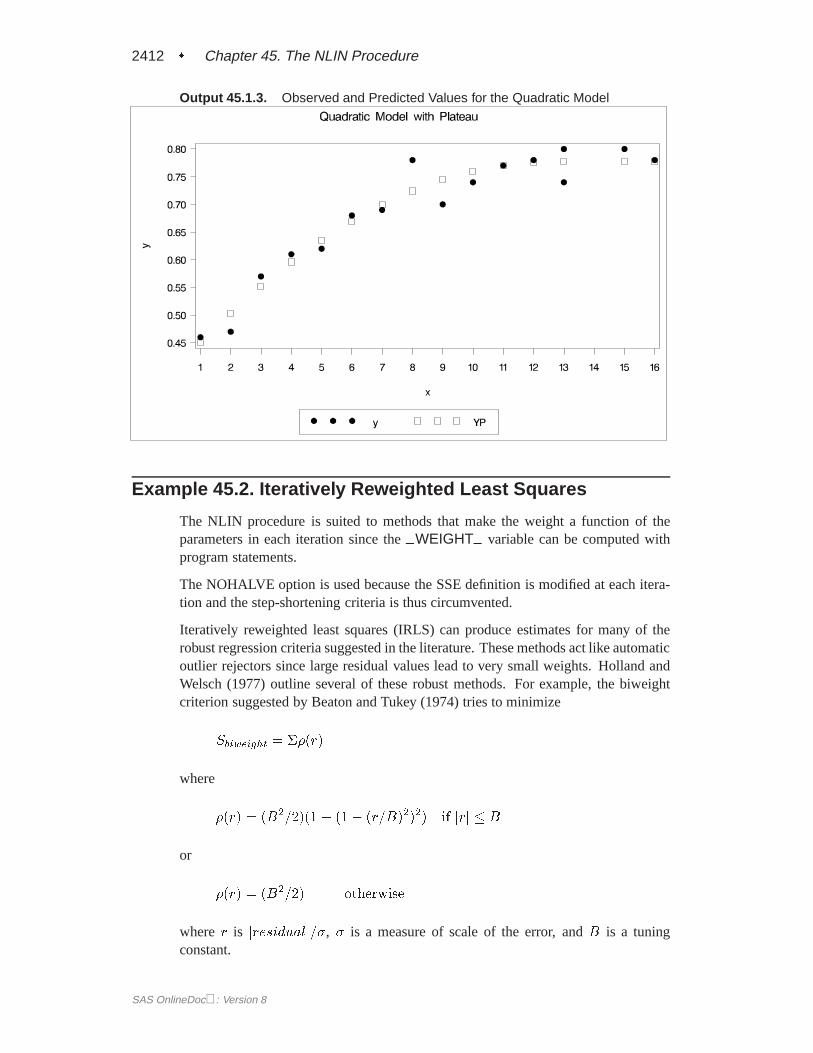
Output 45.1.1 indicates that the join point is 12.75 and the plateau value is 0.78. Asdisplayed in the following plot of the predicted values (YP) and the actual values,the selected join point and plateau value is reasonable. The predicted values for theestimation are written to the data setb with the OUTPUT statement.



Output 45.1.3. Observed and Predicted Values for the Quadratic Model

Example 45.2. Iteratively Reweighted Least Squares

The NLIN procedure is suited to methods that make the weight a function of theparameters in each iteration since the–WEIGHT– variable can be computed withprogram statements.

The NOHALVE option is used because the SSE definition is modified at each itera-tion and the step-shortening criteria is thus circumvented.

Iteratively reweighted least squares (IRLS) can produce estimates for many of therobust regression criteria suggested in the literature. These methods act like automaticoutlier rejectors since large residual values lead to very small weights. Holland andWelsch (1977) outline several of these robust methods. For example, the biweightcriterion suggested by Beaton and Tukey (1974) tries to minimize

Sbiweight = ��(r)

where

�(r) = (B2=2)(1 � (1� (r=B)2)2) if jrj � B

or

�(r) = (B2=2) otherwise

wherer is jresidualj=�, � is a measure of scale of the error, andB is a tuningconstant.


Example 45.2. Iteratively Reweighted Least Squares � 2413

The weighting function for the biweight is

wi = (1� (ri=B)2)2 if jrij � B

or

wi = 0 if jrij > B

The biweight estimator depends on both a measure of scale (like the standard devia-tion) and a tuning constant; results vary if these values are changed.

The data are the population of the United States (in millions), recorded at ten-yearintervals starting in 1790 and ending in 1990.

title ’U.S. Population Growth’;data uspop;

input pop :6.3 @@;retain year 1780;year=year+10;yearsq=year*year;datalines;

3929 5308 7239 9638 12866 17069 23191 31443 39818 5015562947 75994 91972 105710 122775 131669 151325 179323 203211226542 248710;

title ’Beaton/Tukey Biweight Robust Regression using IRLS’;proc nlin data=uspop nohalve;

parms b0=20450.43 b1=-22.7806 b2=.0063456;model pop=b0+b1*year+b2*year*year;resid=pop-model.pop;sigma=2;b=4.685;r=abs(resid / sigma);if r<=b then _weight_=(1-(r / b)**2)**2;else _weight_=0;output out=c r=rbi;

run;

data c;set c;

sigma=2;b=4.685;r=abs(rbi / sigma);if r<=b then _weight_=(1-(r / b)**2)**2;else _weight_=0;

proc print;run;



Output 45.2.1. Nonlinear Least Squares Analysis

Beaton/Tukey Biweight Robust Regression using IRLS

The NLIN Procedure


Regression 3 232436 77478.8 49454.5 <.0001Residual 18 20.6670 1.1482Uncorrected Total 21 232457

Corrected Total 20 113585


b0 20828.7 259.4 20283.8 21373.6b1 -23.2004 0.2746 -23.7773 -22.6235b2 0.00646 0.000073 0.00631 0.00661

Output 45.2.2. Listing of Computed Weights from PROC NLIN


Obs pop year yearsq RBI sigma b r _weight_

1 3.929 1790 3204100 -0.93711 2 4.685 0.46855 0.980102 5.308 1800 3240000 0.46091 2 4.685 0.23045 0.995173 7.239 1810 3276100 1.11853 2 4.685 0.55926 0.971704 9.638 1820 3312400 0.95176 2 4.685 0.47588 0.979475 12.866 1830 3348900 0.32159 2 4.685 0.16080 0.997656 17.069 1840 3385600 -0.62597 2 4.685 0.31298 0.991097 23.191 1850 3422500 -0.94692 2 4.685 0.47346 0.979688 31.443 1860 3459600 -0.43027 2 4.685 0.21514 0.995799 39.818 1870 3496900 -1.08302 2 4.685 0.54151 0.97346

10 50.155 1880 3534400 -1.06615 2 4.685 0.53308 0.9742711 62.947 1890 3572100 0.11332 2 4.685 0.05666 0.9997112 75.994 1900 3610000 0.25539 2 4.685 0.12770 0.9985113 91.972 1910 3648100 2.03607 2 4.685 1.01804 0.9077914 105.710 1920 3686400 0.28436 2 4.685 0.14218 0.9981615 122.775 1930 3724900 0.56725 2 4.685 0.28363 0.9926816 131.669 1940 3763600 -8.61325 2 4.685 4.30662 0.0240317 151.325 1950 3802500 -8.32415 2 4.685 4.16207 0.0444318 179.323 1960 3841600 -0.98543 2 4.685 0.49272 0.9780019 203.211 1970 3880900 0.95088 2 4.685 0.47544 0.9795120 226.542 1980 3920400 1.03780 2 4.685 0.51890 0.9756221 248.710 1990 3960100 -1.33067 2 4.685 0.66533 0.96007

Output 45.2.2 displays the computed weights. The observations for 1940 and 1950are highly discounted because of their large residuals.


Example 45.3. Probit Model with Likelihood function � 2415

Example 45.3. Probit Model with Likelihood function

The data, taken from Lee (1974), consist of patient characteristics and a variableindicating whether cancer remission occured. This example demonstrates how touse PROC NLIN with a likelihood function. In this case, the likelihood function tominimize is

�2 logL = �2NXi=1

wghti log(pi(yi;xi))

where

pi(yi;xi) =

��(�+ �0xi) yi = 01� �(�+ �0xi) yi = 1

and� is the normal probability function. This is the likelihood function for a binaryprobit model. This likelihood is strictly positive so that you can take a square rootof log(pi(yi;xi)) and use this as your residual in PROC NLIN. The DATA step alsocreates a zero-valued dummy variable,like, that is used as the dependent variable.

Data remiss;input remiss cell smear infil li blast temp;label remiss = ’complete remission’;like = 0;label like = ’dummy variable for nlin’;datalines;

1 .8 .83 .66 1.9 1.1 .9961 .9 .36 .32 1.4 .74 .9920 .8 .88 .7 .8 .176 .9820 1 .87 .87 .7 1.053 .9861 .9 .75 .68 1.3 .519 .980 1 .65 .65 .6 .519 .9821 .95 .97 .92 1 1.23 .9920 .95 .87 .83 1.9 1.354 1.020 1 .45 .45 .8 .322 .9990 .95 .36 .34 .5 0 1.0380 .85 .39 .33 .7 .279 .9880 .7 .76 .53 1.2 .146 .9820 .8 .46 .37 .4 .38 1.0060 .2 .39 .08 .8 .114 .990 1 .9 .9 1.1 1.037 .991 1 .84 .84 1.9 2.064 1.020 .65 .42 .27 .5 .114 1.0140 1 .75 .75 1 1.322 1.0040 .5 .44 .22 .6 .114 .991 1 .63 .63 1.1 1.072 .9860 1 .33 .33 .4 .176 1.01 00 .9 .93 .84 .6 1.591 1.02



1 1 .58 .58 1 .531 1.0020 .95 .32 .3 1.6 .886 .9881 1 .6 .6 1.7 .964 .991 1 .69 .69 .9 .398 .9860 1 .73 .73 .7 .398 .986;run;

proc nlin data=remiss method=newton sigsq=1;parms a -2 b -1 c 6 int -10;

/* Linear portion of model ------*/eq1 = a*cell + b*li + c*temp +int;

/* probit */p = probnorm(eq1);

if ( remiss = 1 ) then p = 1-p;

model.like = sqrt(- 2 * log( p));output out=p p=predict;

run;

Note that the asymptotic standard errors of the parameters are computed underthe least squares assumptions. The SIGSQ=1 option on the PROC NLIN state-ment forces PROC NLIN to replace the usual mean square error with 1. Also,METHOD=NEWTON is selected so the true Hessian of the likelihood function isused to calculate parameter standard errors rather than the crossproducts approxima-tion to the Hessian.

Output 45.3.1. Nonlinear Least Squares Analysis from PROC NLIN


The NLIN Procedure

NOTE: An intercept was not specified for this model.


Regression 4 -21.9002 -5.4750 -5.75 .Residual 23 21.9002 0.9522Uncorrected Total 27 0

Corrected Total 26 0


a -5.6298 4.6376 -15.2234 3.9638b -2.2513 0.9790 -4.2764 -0.2262c 45.1815 34.9095 -27.0337 117.4int -36.7548 32.3607 -103.7 30.1879


References � 2417

The problem can be more simply solved using the following SAS statements.

proc probit data=remiss ;class remiss;model remiss=cell li temp ;

run;

References

Bard, J. (1970), “Comparison of Gradient Methods for the Solution of the Nonlin-ear Parameter Estimation Problem,”SIAM Journal of Numerical Analysis, 7,157–186.

Bard, J. (1974),Nonlinear Parameter Estimation, New York: Academic Press, Inc.

Bates, D. M., and Watts, D.L. (1981), “A Relative Offset Orthogonality ConvergenceCriterion for Nonlinear Least Squares”Technometrics, 123, 179-183.

Beaton, A.E. and Tukey, J.W. (1974), “The Fitting of Power Series, Meaning Poly-nomials, Illustrated on Band-Spectroscopic Data,”Technometrics, 16, 147–185.

Charnes, A., Frome, E.L., and Yu, P.L. (1976), “The Equivalence of GeneralizedLeast Squares and Maximum Likelihood Estimation in the Exponential Family,”Journal of the American Statistical Association, 71, 169–172.

Cox, D.R. (1970),Analysis of Binary Data, London: Chapman and Hall.

Finney, D.J. (1971),Probit Analysis, Third Edition, Cambridge: Cambridge Univer-sity Press.

Gallant, A.R. (1975), “Nonlinear Regression,”American Statistician, 29, 73–81.

Gill, Philip E., Murray, Walter, and Wright, Margaret H. (1981), "Practical Optimiza-tion," New York: Academic Press Inc.

Hartley, H.O. (1961), “The Modified Gauss-Newton Method for the Fitting of Non-Linear Regression Functions by Least Squares,”Technometrics, 3, 269–280.

Holland, P.H. and Welsch, R.E. (1977), “Robust Regression Using IterativelyReweighted Least-Squares,”Communications Statistics: Theory and Methods,6, 813–827.

Jennrich, R.I. (1969), “Asymptotic Properties of Nonlinear Least Squares Estima-tors,” Annals of Mathematical Statistics, 40, 633–643.

Jennrich, R.I. and Moore, R.H. (1975), “Maximum Likelihood Estimation by Meansof Nonlinear Least Squares,”American Statistical Association, 1975 Proceedingsof the Statistical Computing Section, 57–65.

Jennrich, R.I. and Sampson, P.F. (1968), “Application of Stepwise Regression to Non-Linear Estimation,”Technometrics, 10, 63–72.

Judge, G.G., Griffiths, W.E., Hill, R.C., and Lee, Tsoung-Chao (1980),The Theoryand Practice of Econometrics, New York: John Wiley & Sons, Inc.



Kennedy, W.J. and Gentle, J.E. (1980),Statistical Computing, New York: MarcelDekker, Inc.

Lee, E.T. (1974), “A Computer Program for Linear Logistic Regression Analysis,”Computer Programs in Biomedicine, 80–92.

Marquardt, D.W. (1963), “An Algorithm for Least-Squares Estimation of NonlinearParameters,”Journal for the Society of Industrial and Applied Mathematics, 11,431–441.

Nelder, J.A. and Wedderburn, R.W.M. (1972), “Generalized Linear Models,”Journalof the Royal Statistical Society, Series A, 135, 370–384.

Ralston, M.L. and Jennrich, R.I. (1978), “DUD, A Derivative-Free Algorithm forNonlinear Least Squares,”Technometrics, 20, 7–14.

Ratkowsky, D. (1990), "Handbook of Nonlinear Regression Models," Marcel Dekker:New York and Basel.


The correct bibliographic citation for this manual is as follows: SAS Institute Inc.,SAS/STAT ® User’s Guide, Version 8, Cary, NC: SAS Institute Inc., 1999.

SAS/STAT® User’s Guide, Version 8Copyright © 1999 by SAS Institute Inc., Cary, NC, USA.ISBN 1–58025–494–2All rights reserved. Produced in the United States of America. No part of this publicationmay be reproduced, stored in a retrieval system, or transmitted, in any form or by anymeans, electronic, mechanical, photocopying, or otherwise, without the prior writtenpermission of the publisher, SAS Institute Inc.U.S. Government Restricted Rights Notice. Use, duplication, or disclosure of thesoftware and related documentation by the U.S. government is subject to the Agreementwith SAS Institute and the restrictions set forth in FAR 52.227–19 Commercial ComputerSoftware-Restricted Rights (June 1987).SAS Institute Inc., SAS Campus Drive, Cary, North Carolina 27513.1st printing, October 1999SAS® and all other SAS Institute Inc. product or service names are registered trademarksor trademarks of SAS Institute Inc. in the USA and other countries.® indicates USAregistration.Other brand and product names are registered trademarks or trademarks of theirrespective companies.The Institute is a private company devoted to the support and further development of itssoftware and related services.

Documents

The NLIN Procedure