Embed Size (px)
Citation preview
THE NEW ECONOMICS OF EQUILIBRIUM SORTING
AND ITS TRANSFORMATIONAL ROLE FOR POLICY EVALUATION
Nicolai V. Kuminoff Assistant Professor
Department of Economics Arizona State University
V. Kerry Smith W.P. Carey Professor
Department of Economics Arizona State University
Christopher Timmins Associate Professor
Department of Economics Duke University
August 2010
THE NEW ECONOMICS OF EQUILIBRIUM SORTING
AND ITS TRANSFORMATIONAL ROLE FOR POLICY EVALUATION
ABSTRACT: Households “sort” across neighborhoods according to their wealth and their preferences for public goods, social characteristics, and commuting opportunities. The aggrega-tion of these individual choices in markets and in other institutions influences the supply of amenities and local public goods. Pollution, congestion, and the quality of public education are examples. Over the past decade, advances in economic models of this sorting process have led to new framework that promises to alter the ways we conceptualize the policy evaluation process in the future. These “equilibrium sorting” models use the properties of market equilibria, togeth-er with information on household behavior, to infer structural parameters that characterize preference heterogeneity. The results can be used to develop theoretically consistent predictions for the welfare implications of future policy changes. Analysis is not confined to marginal effects or a partial equilibrium setting. Nor is it limited to prices and quantities. Sorting models can integrate descriptions of how non-market goods are generated, estimate how they affect decision making and, in turn, predict how they will be affected by future policies targeting prices or quantities. Conversely, sorting models can predict how equilibrium prices and quantities will be affected by policies which target product quality, information, or amenities generated by the sorting process. These capabilities are just beginning to be understood and used in applied research. This survey article aims to synthesize the state of knowledge on equilibrium sorting, the new possibilities for policy analysis, and the conceptual and empirical challenges that define the frontiers of the literature.
KEY WORDS: Equilibrium sorting, hedonic, endogenous amenities, heterogeneity, policy
evaluation JEL NO: H41, D61, Q50

1. Introduction
Economists use sorting as a metaphor for the way that market forces partition economic agents
across segments of a market. Households “sort” across neighborhoods according to their wealth
and their preferences for public goods, social characteristics, and commuting opportunities.
Workers “sort” across jobs according to their qualifications and preferences for job attributes. In
situations with other differentiated products such as automobiles, breakfast cereal, and comput-
ers, we expect that consumers who have similar preferences and face similar constraints will
make similar choices. This sorting process reveals information about consumers, and firms have
learned to exploit it to increase their profits. They design differentiated products and set prices
to take advantage of what is known about consumer heterogeneity. Knowledge of consumer
heterogeneity can also be used to evaluate past policies and design new ones. This is especially
important for policy targeting public goods and externalities. The challenge for economists is to
describe sorting behavior and learn from it. Our models need to reflect the information available
to the agents involved, their constraints, and the implications of their collective actions for
market and non-market outcomes.
Over the past decade, advances in economic models of sorting have led to a new frame-
work for policy evaluation. These “equilibrium sorting” models use the properties of market
equilibria, together with information on the behavior of economic agents, to infer structural
parameters that characterize agent heterogeneity. The results can be used to develop theoretical-
ly consistent predictions for the welfare implications of future policy changes. Analysis is not
confined to marginal effects or a partial equilibrium setting. Nor is it limited to prices and
quantities. As heterogeneous agents sort, their collective behavior can influence the supply of
amenities. These adjustments can be represented as part of the characterization of the equilibria
and influence its properties. Pollution, congestion, and opportunities for social interaction
provide examples. Sorting models can integrate descriptions of how these amenities are generat-
ed, estimate how they affect decision making and, in turn, predict how they will be affected by
future policies targeting prices or quantities. Conversely, sorting models can predict how
equilibrium prices and quantities will be affected by policies which target product quality,
information, or amenities generated by the sorting process. These capabilities are just beginning
to be understood and used in applied research.
Equilibrium sorting models build on the intellectual foundations of the literature on he-
2
donic and discrete-choice models of differentiated product markets. They combine the informa-
tion provided by an equilibrium hedonic price function (Sherwin Rosen 1974; Dennis Epple
1987; Ivar Ekeland, James J. Heckman, and Lars Nesheim 2004) with a formal description for
the choice process that underlies market sorting of heterogeneous agents (Daniel McFadden
1974; Timothy Bresnahan 1987; Steven Berry, James Levinsohn, Ariel Pakes 1995). This
equilibrium sorting framework can depict a mixture of discrete and continuous choices made by
a population of heterogeneous agents, while recognizing that characteristics of the objects of
choice may be determined endogenously (Epple and Holger Sieg 1999; Patrick Bayer and
Christopher Timmins 2005, 2007).
What ideas distinguish the economics of equilibrium sorting from past strategies for
modeling differentiated goods? First, in addition to characterizing sources of unobserved
heterogeneity such as technology and preferences, they include a wide array of observable
features that distinguish economic agents. These observable dimensions of agent heterogeneity
can be used in descriptions of sorting behavior and are often especially important in characteriz-
ing the implications of polices. Through the sorting process, that heterogeneity is translated into
endogenously determined attributes of the choice alternatives available to agents. In the housing
market, for example, the attributes of the neighborhoods that a household chooses from may
depend on where its primary earner works, while its preferences for school districts may depend
upon the levels of education attained by the adult members of the household. As households
with different incomes and levels of education decide where to live, they will influence the
demographic compositions of neighborhoods. When households vote, their preferences will
shape public policies that influence school quality, open space, and congestion. The supply of
each of these amenities is thus determined endogenously–as an outcome of the sorting process.
This creates an econometric problem for researchers simply interested in recovering consistent
estimates of households’ preferences.
Endogenous amenities will also influence market outcomes for private goods, such as
housing prices and wage rates. This creates a second distinction between the economics of
equilibrium sorting and earlier models of the demand for differentiated products. In particular,
the sorting literature seeks to understand “general equilibrium” feedback effects between eco-
nomic agents and their environments. For example, a shock to the housing market that induces a

3
change in residential location patterns may lead to a redistribution of local amenities that induces
more migration and housing development which continues until prices adjust and markets clear.
Modeling these feedback effects is important for researchers interested in simulating the impacts
of a counterfactual policy.
Third, the equilibrium sorting literature considers how public policies can be designed to
exploit what we learn about forms of heterogeneity, endogeneity, and feedback. Some time ago,
Alan S. Blinder and Harvey S. Rosen (1985) demonstrated how information about preference
heterogeneity could, in principle, be used to design more efficient taxes on private goods.
Emmanuel Saez (2010) recently used a similar logic to test whether workers respond to nonli-
nearities in the tax code. Equilibrium sorting models provide the means to implement both the
original Blinder-Rosen idea and the Saez test and extend them to the consideration of policies
that target public goods or other amenities that affect agents differently.
Applications of the new models have demonstrated that agent heterogeneity, endogenous
attributes, and feedback effects can all have first-order policy implications (Sieg et al. 2004; V.
Kerry Smith et al. 2004; Maria Marta Fererrya 2007; Timmins 2007; Randall L. Walsh 2007;
Nicolai V. Kuminoff 2009; H. Allen Klaiber and Daniel J. Phaneuf 2010b; Constant I.Tra 2010).
These studies investigate how sorting behavior in housing markets relates to air quality, school
quality, open space, climate, and other amenities. One of the policy-relevant insights is that the
properties of market equilibria can depend on feedback effects which occur through non-market
transmission routes. For example, in Walsh (2007) households get utility from access to open
space, which decreases as new houses are built in a closed community. This non-market feed-
back effect causes each household’s location choice to depend on the choices made by other
households. The demand side of a sorting equilibrium that clears this market is itself a Nash
equilibrium that fits within the class of aggregative public goods games characterized by Richard
Cornes and Roger Hartley (2007). Sorting in response to feedback leads to a surprising result in
Walsh’s policy simulation. Increasing the amount of land in public preserves can actually
decrease the total amount of land in open space in the metro area. The mechanisms that produce
this outcome mirror a counterintuitive result from Matthew J. Kotchen’s (2006) theoretical
model of Nash equilibria in green markets.
Housing markets provided the testing ground for equilibrium sorting models. The mod-

4
els were initially developed to deal with features of the homebuyer’s location choice problem
that were difficult to address using conventional methods. The resulting techniques have been
used to study behavior in a wide range of differentiated product markets. Recent applications
have considered network effects (Marc Rysman 2004; Shanjun Li 2006), location choices of
firms (Katja Seim 2006), markets for education (Epple, Richard Romano, and Sieg 2006, 2010),
social interactions in labor markets (Bayer, Steve Ross, and Giorgio Topa 2008), and the impact
of congestion on recreation demand (Timmins and Jennifer Murdock 2007).
The potential for using equilibrium sorting models to conduct high-resolution policy
analysis is exciting, but are their predictions reliable? Over the past decade the profession has
become increasingly skeptical of structural modeling (Joshua D. Angrist and Jörn-Steffen
Pischke 2010). This skepticism reinforces the need to understand how the features of structural
models contribute to their identification of welfare measures and other policy implications
(Michael Keane 2010). The equilibrium sorting literature has addressed some of the traditional
criticisms of structural modeling by developing nonlinear and semiparametric estimators that
allow functional forms and distributional assumptions to be selected based on data and theory
rather than computational convenience. Nonetheless, to characterize the sorting process, model-
ing judgments must be made and these can influence policy implications. For example, different
researchers have suggested competing specifications for preference functions and the form of
agent heterogeneity which, in turn, differ in their implications for substitution possibilities and
welfare estimates. Furthermore, in order to quantify the implications of a non-marginal policy
change, an equilibrium selection rule may need to be formulated. Given the current debates
about the assumptions being made in quasi-experimental versus structural models, questions
about the relevance of the former for policy evaluation, and the recent developments in the
structural sorting literature, the time is right to pause and identify what we have learned, the
problem areas, and the puzzles that remain. This survey article aims to synthesize the state of
knowledge on equilibrium sorting, the new possibilities for policy analysis, and the conceptual
and empirical challenges that define the frontiers of the literature.
We concentrate on research in public and environmental economics, with particular atten-
tion to the market for housing. Models of household location choice build on theory and me-
thods developed in related fields, especially industrial organization and labor economics. We

5
highlight connections to work in those areas, without providing a comprehensive assessment.
Our focus is on recent research. While we do not present a complete historical perspective, it
should be noted that much of the work we cover was influenced by the seminal papers written by
Charles M. Tiebout (1956), William Alonso (1964), John Krutilla (1967), Edwin S. Mills (1967),
Richard F. Muth (1969), Wallace E. Oates (1969), Thomas C. Schelling (1969), and Edwin T
Haefele (1971).
Our survey begins by describing the foundations of the new equilibrium sorting literature
in section 2, from early median voter models of the demand for public goods to the modern
discrete choice framework for describing how households sort over neighborhoods. Section 3
covers the evolution of sorting theory. This line of research has sought to characterize multi-
community equilibria with peer effects, voting, and other forms of social interaction. The
implied relationship between property values, housing characteristics, and local public goods can
be described by a hedonic price function. Empirical models use properties of sorting equilibria
to recover household preferences and estimate the demand for public goods. These models can
be divided into two broad frameworks. Section 4 covers hedonic models, most of which take a
reduced-form (and increasingly quasi-experimental) approach to estimation. Section 5 covers
structural models of sorting behavior. In section 6 we contrast how hedonic and sorting models
are used to evaluate public policy. Leading examples are provided (education, air pollution, and
land use) and we conclude with an assessment of how the new sorting models can improve future
evaluations. Finally, section 7 concludes by identifying current frontiers of the literature.
2. Foundations and Motivation
Empirical sorting models are motivated by a long-standing question. How can we esti-
mate the demand for public goods that are not explicitly traded in formal markets? Early re-
search sought to estimate demand by simply regressing expenditures for municipal services on
the characteristics of voters. Tiebout (1956) recognized that households “vote with their feet”.
These migration patterns can bias reduced-form estimation. Mitigating the bias requires know-
ledge of the sorting process that underlies market equilibrium. This realization led to subsequent
research on characterizing the properties of equilibria that result from heterogeneous households

6
sorting themselves across differentiated communities. Formal models of the sorting process
were developed using the characteristics approach to consumer theory (Kelvin J. Lancaster 1966;
William M. Gorman 1980).
The remainder of this section describes the foundations of the new equilibrium sorting li-
terature, from the early reduced form studies to the modern characteristics framework, and
summarizes the features of the location choice problem that differentiate the resulting theory and
econometrics from characteristics based models of the demand for differentiated products.
2.1 A Reduced-Form Approach to Estimating the Demand for Public Goods
Theodore C. Bergstrom and Robert P. Goodman (1973) were among the first to propose a
strategy for estimating the demand for local public goods. They envisioned an urban landscape
in which the level of public goods supplied by each community is determined by that communi-
ty’s median voter. Assuming the median voter also has the median level of income, the demand
for a public good can be estimated by simply regressing actual public good expenditures (A) on
the incomes ( medy ) and marginal tax rates ( medτ ) faced by the median household in each of
several communities,
(1) ∑ ++++=k
medmedkkmedmed udyA ,210 lnlnln βτβββ ,
where the sdk ' describe the median household’s demographic characteristics. The simplicity of
Bergstrom and Goodman’s estimator inspired numerous applications to community level data, as
well as a microeconometric extension of the model to individual survey data (Bergstrom, Daniel
L. Rubinfeld and Perry Shapiro 1982).
The problem with estimation of (1) is that it ignores the sorting process that underlies
equilibrium in the market for housing. If households choose where to live based, in part, on their
preferences for public goods, the community selection mechanism can bias estimation of the
price and income elasticities. Gerald S. Goldstein and Mark V. Pauly (1981) labeled this prob-
lem “Tiebout bias” after Tiebout’s (1956) conceptual model of local public goods provision.1
1 Tiebout (1956) envisioned freely mobile households migrating across communities based on their preferences for the public goods provided by those communities. This type of sorting behavior poses a problem for OLS estimation

7
To illustrate Tiebout bias, we draw on an example from Rubinfeld, Shapiro and Judith
Roberts (1987). Suppose household i maximizes its utility by locating in one of a discrete set of
J communities based, in part, on its preferences for public goods,
(2) ( )iijjjJjdyAVj ,,, max τ
∈= .
Then the estimating equation from Bergstrom and Goodman’s (1973) model can be rewritten for
an individual observation as
(3) ∑ ++++=k
jijikkjijiji udyA ,,,,2,10, lnlnln βτβββ .
Reformulating the problem in terms of individual behavior allows us to interpret the econometric
error term as a function of unobserved preferences. In this context, preference based sorting
presents a simultaneity problem. That is, household incomes and property taxes may be influ-
enced by the sorting process in (2). A household’s income will depend on its location choice if
communities differ in the job opportunities they provide. A community’s marginal tax rate will
depend on the composition of its residents if tax rates are determined by voting. If income and
taxes depend on location choices that are driven, in part, by unobserved preferences, jiu , will be
correlated with jiy , and ji,τ , biasing OLS estimation of (3).
Rubinfeld, Shapiro, and Roberts (1987) propose a two-step selection model that has the
potential to provide consistent estimates of the demand for a public good in the presence of
Tiebout bias. While the logic behind their estimator is straightforward, there is a major hurdle to
implementation—it requires instruments for the endogenous variables in (3). This requirement
creates a challenge because the validity of any potential instrument depends on the ways in
which the sorting of heterogeneous households influences the properties of equilibria. Put
differently, to evaluate the validity of a potential instrument, one must provide a full specifica-
tion of the sorting equilibrium. Thus, developing consistent estimates of the demand for a public
good requires knowledge of the sorting process.
of (1) regardless of whether the data describe the median household in each community or a random sample of households.

8
2.2 A Model of Household Location Choice
Equilibrium models of Tiebout sorting begin with a simple premise: the amount and cha-
racter of housing and public goods varies across an urban landscape, and each household selects
its preferred bundle of public and private goods given its income and the relative prices involved.
Every household pays for its location choice through the price of housing. Working households
may also pay indirectly through the wages they earn. In order to link a household’s location
choice to its preferences for an individual public good, the problem is formalized using the
characteristics approach to consumer theory developed by Lancaster (1966) and Gorman (1980).
The appendix provides a reference guide to the notation that we use.
Assume the urban landscape consists of Nn ,....,1= houses that can be divided into
Jj ,....,1= communities. Each home can be defined by a bundle of housing characteristics and
amenities. nh is a vector of structural characteristics that fully describe the private good compo-
nent of an individual home. For example, nh could include the number of bedrooms, the number
of bathrooms, square feet, and lot size. jg denotes a vector of amenities conveyed to every
household in community j. It may include local public goods such as school quality, urban and
environmental services (such as crime rates, and air quality), and variables describing the demo-
graphic composition of the community (such as race, educational attainment). We will use the
term “amenities” to refer to any of these non-market goods and services.
A household’s utility depends on the characteristics of housing and amenities at its loca-
tion and on its consumption of a composite numeraire private good, b. Households are heteroge-
neous. They differ in unobservable features of their preferences ( )α and in observable factors
such as their demographic characteristics ( )d . Let the population of households be indexed from
Ii ,....,1= . The utility obtained by household i from house n in community j can be represented
as: ( )iijn dghbU ,;,, α .2
Each household is assumed to choose a location and a quantity of b that maximize its util-
ity subject to a budget constraint:
2 A household may contain many members with different demographic characteristics and preferences, but it is treated as an indivisible economic agent.

9
(4) ( ) jnjiiijnbjnPbytosubjectdghbU ∈∈
+=,,,;,,max α .
In the budget constraint, the price of the numeraire is normalized to one and jnP∈ represents
annualized expenditures on house n in community j; in other words, jnP∈ is the after-tax cost of
occupying a single home for one year.3jiy , is the household’s total annual income. The j
subscript on income recognizes that, in general, income is endogenous to location choice. In
particular, wages will be endogenous if heterogeneous workers sort across a landscape with
spatial variation in the composition of labor demand. Even if employment locations are fixed,
income may be endogenous to the housing location decision because of commuting costs.
The specification in (4) implicitly removes three potential sources of “friction” from the
problem. First, all households are assumed to share the same objective evaluation of housing
characteristics and amenities. Second, households are assumed to be freely mobile within the
geographic region defined as the choice set. Third, every household is assumed to face the same
schedule of housing prices. These three assumptions—full information, free mobility, and no
discrimination—are maintained in the literature with very few exceptions.
Equilibrium is achieved when every household occupies its utility-maximizing location
and nobody wants to move, given housing prices, housing characteristics, wages, tax rates, and
the levels of each amenity. The literature can be organized around this concept. Theoretical
models investigate the existence and uniqueness of equilibria and their implications for equity
and efficiency. Empirical models use the properties of equilibria to infer preferences for ameni-
ties from the observable characteristics of households and their location choices. Finally,
because empirical models can be estimated in a way that characterizes equilibrium in the entire
housing market, the estimation results can be used to predict market responses to policies that
would make large scale changes to amenities.4
3 This interpretation is also an important part of the logic for Epple, Brett Gordon, and Sieg’s (2010) new approach to estimating the supply of housing, discussed in section 7.3. 4 In this context, a “prediction” simply describes what the model would imply for the equilibrium, given some counterfactual conditions. These predictions have been used to evaluate the types of responses that would be expected to follow specific policy changes. They have not been used to develop forecasts for future housing market conditions.5 For example, Phaneuf et al. (2008) link a model of building activity to a spatial model of a river system in order to assess the marginal damages of water pollution due to that construction.

10
2.3 Distinguishing Features of the Household’s Location Choice Problem
The structure of the location choice problem is quite similar to the structure of differen-
tiated product models in other fields. At an abstract level, equation (4) simply depicts heteroge-
neous agents choosing among a set of differentiated objects to satisfy their idiosyncratic tastes.
Because of this common foundation, the theory and methods that were initially developed to
model households’ location choices were built on work in related domains, especially industrial
organization and labor economics.
Four features of the homebuyer’s location choice problem presented new modeling chal-
lenges. First, location choices are differentiated by a mixture of public and private goods.
Second, some of the public goods are endogenously determined by the sorting process. Third,
sorting arises, in part, from the combination of heterogeneity in preferences and heterogeneity in
the spatial landscape. Finally, with endogenous characteristics and heterogeneous preferences,
there can be multiple equilibria. Before turning to the theory and econometrics of equilibrium
sorting, we briefly explain these distinguishing features of the problem.
2.3.1 A Mixture of Public and Private Characteristics
Differentiated product models in industrial organization tend to focus on private goods
defined by characteristics that are rivalrous and excludable such as automobiles (Berry, Levin-
sohn, and Pakes 1995), breakfast cereal (Aviv Nevo 2001), computers (Patrick Bajari and Lanier
Benkard 2005), and laundry detergent (Igal Hendel and Nevo 2006). Recreation demand studies
investigate how people choose among public goods such as lakes and parks, which may be
differentiated by their opportunities for fishing and boating (Phaneuf and Smith 2005). These
services are non-rival until a capacity level is reached, at which point their quality becomes a
function of congestion (Timmins and Murdock 2007). In the homebuyer’s location choice
problem, some attributes are rival, some are not, and some depend on congestion.
As heterogeneous households sort themselves across the spatial landscape, their collec-
tive behavior can affect the supply of club goods and open access resources which, in turn,
become part of the characterization of the equilibria and influence its properties. What are the
implications of this process for the efficiency of equilibria? Does it impair our ability to identify

11
the demand for characteristics? Can we exploit the complementarity between public and private
characteristics to design more effective policies? The answers to these questions depend on our
understanding of the mechanisms that determine the supply of endogenous characteristics.
2.3.2 Endogenous Characteristics The recognition that characteristics of the object of choice may be endogenously deter-
mined through the market clearing process is perhaps the single most important feature to
distinguish the equilibrium sorting literature from the broader literature on differentiated prod-
ucts. The level of an amenity can be determined through social choice, social interaction, or
feedback effects. Consider the case of social choice. Expenditures on local public goods are
determined by voting. Residents of each community vote on property tax rates and on special
assessments that aim to provide additional funding for schools, law enforcement, and other
services. This is the Bergstrom and Goodman (1973) logic for their median voter model cited
earlier.
While voting may determine expenditures on local public goods, their quality may be
determined by social interactions. For example, the quality of a school is often judged by how
its students perform on standardized tests. The best predictors of a student’s performance tend to
be the demographic characteristics of her parents (particularly income and education) and the
performances of her peers (Eric A. Hanushek 2003). Thus, peer effects make the level of school
quality a function of the demographic characteristics of the parents who live in that district.
Social interactions can also influence the demographic composition of a community and
the services it provides. If people care about the ethnicity of their neighbors (or other characte-
ristics such as age, race, and wealth) then the sorting process that determines community demo-
graphics will reflect these social interactions. For example, David M. Cutler, Edward L. Glaeser,
and Jacob L. Vigdor (1999) conclude that patterns of racial segregation in 1990 are best ex-
plained by whites preferring to live in predominantly white communities.
Household location choices can also generate feedback effects that affect the quality of
environmental services. As people with strong preferences for open space move into a metropol-
itan area, the remaining open space gets developed for additional housing. Increases in pave-

12
ment generate urban heat islands. Runoff of lawn fertilizer from the newly built subdivisions
may cause water quality to decline.5
The corresponding increase in automobile traffic may
decrease air quality. As these feedback effects alter the metropolitan landscape, the environmen-
tal amenities that initially attracted households to the area may be degraded.
2.3.3 Heterogeneity in Preferences and the Spatial Landscape
Spatial stratification constrains the production and consumption of goods. To consume
the amenities provided by a community, a household must move there. The scope for its resi-
dents to influence those amenities is defined, in part, by boundaries such as school districts,
voting jurisdictions, and air basins. The characteristics of the resulting spatial equilibrium will
reflect the distribution of preferences in the population of households. Tiebout (1956) reasoned
that, with spatial variation in amenities and free mobility, the location choices that households
make reveal their preferences. In his own words: “There is no way in which the consumer can
avoid revealing his preferences in a spatial economy. Spatial mobility provides the local public-
goods counterpart to the private market’s shopping trip.” A number of authors contributed to
formalizing Tiebout’s logic, as we discuss in the next section. In particular, Epple’s research
with a variety of collaborators provided the initial basis for understanding how preference
heterogeneity influences spatial variation in the supply of amenities, yielding equilibria that can
be used to recover information about those preferences.
Bayer and Timmins (2007) demonstrated that our ability to identify preferences can be
enhanced by instrumental variables developed from our knowledge of the spatial distribution of
endogenous and exogenous amenities. Information about preferences is needed to predict how
new policies will affect features of the spatial equilibrium. Simon P. Anderson, André de Palma,
and Jaques-François Thisse (1992) formalized one dimension of this argument, demonstrating
that the structure of preference heterogeneity will determine the substitutability between diffe-
rentiated objects of choice (in our case, communities).
5 For example, Phaneuf et al. (2008) link a model of building activity to a spatial model of a river system in order to assess the marginal damages of water pollution due to that construction.

13
2.3.4 Multiplicity of Equilibria
Because equilibrium sorting models provide a characterization of the equilibrium, we
have the ability to predict how the supply of an endogenous amenity will adjust to a new policy
that targets housing prices or quantities. Conversely, we can predict how equilibrium prices and
quantities will be affected by policies which target amenities. To assess these effects, however,
we must first solve for the new equilibrium that would follow a prospective policy shock. This
task presents theoretical and computational challenges.
When households have heterogeneous preferences for multiple amenities there can be
multiple equilibria. Analytical proofs of uniqueness can only be obtained by adding restrictions
to the structure of preferences or by limiting the number of endogenous amenities. Without these
restrictions, different equilibria may be compared on the basis of their stability, their implications
for market efficiency, or their welfare implications for particular demographic groups. Which
equilibrium emerges after a policy shock may depend on the market institutions that govern
transitional dynamics. Research on the theory and methods associated with sorting dynamics is
one of the current research frontiers.
3. Equilibrium Sorting Theory
The theoretical literature that followed Tiebout’s early work focused on formalizing his
conceptual model, proving the existence of an equilibrium in which no household would be
better off by moving, and extending his framework to include peer effects and other forms of
social interaction within communities. Part 1 of this section summarizes a series of articles that
develop increasingly general depictions of sorting equilibria. Part 2 adds social interactions and
discusses the implications for equity and efficiency. Part 3 describes the hedonic price function
that characterizes the equilibrium relationship between property values, housing characteristics,
and spatially differentiated amenities.
3.1 Equilibrium Stratification Patterns
For heuristic purposes, a household’s choice process can be depicted as a two-stage prob-
lem where each household first determines the optimal quantities of housing and numeraire in

14
each of a finite number of communities, and then chooses the particular community that max-
imizes its utility.6
(5)
The first stage is
( ) hpbytosubjectghbU jjbh⋅+=α,,,max
,.
Theoretical models usually treat housing as a homogeneous commodity that can be consumed in
continuous quantities at a constant price. This is represented in (5) by defining jp as the annual-
ized per-unit price of housing in community j and h as the quantity of housing consumed. Note
that the bar on h does not imply the quantity of housing consumed is fixed; the quantity con-
sumed may vary across households according to their income, preferences, and chosen commu-
nity. The bar superscript is meant to differentiate the concept of a homogeneous unit of housing
from h , which continues to represent a vector of specific structural characteristics (e.g. bed-
rooms, bathrooms, square feet).7
Assuming households can purchase any quantity of housing at the market price in each
community, housing is “optimized out” of the problem and preferences can be restated using the
indirect utility function in (6).
(6) ( ) ( ) ( )[ ]αααα ,,,,,,,,,,,, ypghpyypghgUypgV ⋅−= .
Each household will choose the community that maximizes its well-being, given income and
prices. A sorting equilibrium is achieved when every household has chosen its utility-
maximizing community and nobody wants to move, given housing prices and the level of local
public goods.
Bryan Ellickson (1971) first characterized the restrictions on preferences that would sup-
port the existence of sorting equilibria. Three features of his model form the basis for most of
the subsequent studies. First, he assumed that provision of public goods in community j could be
represented by a 1-dimensional measure, jg , an index that represents the composite quality of
public goods in that community. Second, he assumed that households have homogeneous
6 We have dropped the d term describing the individual’s observable demographic characteristics at this stage to simplify notation. 7 This is one strategy for restricting the general specification used to estimate household preferences from data on housing transactions. In the “pure characteristics” approach to estimation, covered in section 5.1, housing expendi-tures are translated into a price index for homogenous housing using an approach developed by Sieg et al. (2002).

15
preferences ( )Ii αα == ... and therefore differ only in their income. Given the first two assump-
tions, he imposed the restriction that indifference curves in the ( )pg , plane are strictly increas-
ing in income. This, he reasoned, would support a sorting equilibrium in which households are
perfectly stratified across communities by income. Figure 1 uses a two-community example to
illustrate the idea. Household i is exactly indifferent between the two communities. Any
household with lower income, such as household 1−i , will always prefer the cheaper communi-
ty because indifference curves cannot cross more than once. Conversely, any household with
higher income, such as 1+i , will always prefer the more expensive community.
Using the three restrictions from Ellickson’s paper, Frank Westoff (1977) proved that a
sorting equilibrium exists in a model where households in each community vote to determine
public goods provision and community-specific tax rates. Epple, Radu Filimon, and Thomas
Romer (1984, 1993) extended Westoff’s model to include a market for housing that must clear
within each community. Finally, Epple and Romer (1991) generalized the model further to allow
voters to anticipate the consequences of their votes for housing prices and migration. While
these models help to formalize Tiebout’s theory, they do a poor job of reproducing the actual
sorting behavior that we observe. To see why, let the J communities be ordered by their quality
of public goods provision: Jggg <<< ...21 . The key restriction in the early theoretical litera-
ture—Ellickson’s single-crossing restriction—implies that households are partitioned across
communities by income, as illustrated in figure 2. In the figure, every household in community 1
has lower income than every household in community 2, and so on. This characterization is a
poor approximation to reality. That is, actual community-specific income distributions overlap
substantially.
One explanation for why households do not perfectly stratify by income is that they differ
in their tastes for public goods. Recognizing this, Epple and Glen J. Platt (1998) extended the
Epple-Romer model to allow households to differ in a single heterogeneous parameter that
represents their preferences for composite provision of public goods relative to private goods. In
this case, equilibrium is characterized by a more general version of Ellickson’s single-crossing
restriction. To formalize the restriction, equation (7) shows the slope of an “indirect indifference
curve” in ( )pg , space.

16
(7) ( ) ( )( ) pypgV
gypgVVVgd
dpypgM∂∂∂∂
−===,,,,,,,,,
ααα .
Assuming M is monotonically increasing in ( )α|y and ( )y|α , indifference curves in the ( )pg ,
plane satisfy single crossing. This has an intuitive interpretation. Roy’s Identity implies that
( ) pV ∂⋅∂− must equal the marginal utility of income, ( ) yV ∂⋅∂=λ , times the Marshallian
demand for housing, ( )ypgh ,,, α .
(8) ( ) ( )( )
( )( ) ( )
( )( )
∂⋅∂∂⋅∂
⋅=
⋅∂⋅∂
=∂⋅∂∂⋅∂
−=⋅yVgV
hhgV
pVgVM 1
λ.
The term in brackets in equation (8) is the Marshallian virtual price of public goods. Therefore,
the single crossing restriction implies that the Marshallian virtual price, per unit of housing, is
strictly increasing in income and in preferences for public goods relative to private goods.8
The single crossing condition implies that, in equilibrium, three properties characterize
sorting by each household type: boundary indifference, stratification, and increasing bundles
(Epple and Platt 1998). Without loss of generality, let the J communities be ordered according to
the index of public goods,
Jgg << ...1 . Boundary indifference requires a household on the
“border” between two communities in ( )y,α space to be exactly indifferent between those
communities. Equation (9) defines the set of border individuals. It must hold for all
1,...,1 −= Jj .
(9) ( ) ( ) ( ) ypgVypgVy jjjj ,,,,,,:, 11 ααα ++= .
The increasing bundles property requires that for any two communities in the ordering, ( )1, +jj
equation (10) must hold.
(10) ( ) ( ) jjjjjj ggandppyy >>⇒> +++ 111 αα .
That is, the ranking of communities by public goods provision must match the ranking by price.
8 This property is related to the Willig condition that is often applied together with weak complementarity to identify the Hicksian willingness to pay for changes in public goods. The Willig condition requires the willingness-to-pay per unit of the weak complement to be constant at all levels of income. See Smith and H. Spencer Banzhaf (2004, 2007) and Raymond B. Palmquist (2005) for details. David S. Bullock and Nicholas Minot (2006) have demonstrat-ed that the Willig condition is sufficient but not necessary for identifying willingness to pay for changes in non-market goods with weak complementarity.

17
The third property, stratification, requires that households of each type are stratified across the J
ordered locations by ( )y|α and by ( )α|y , as defined in (11).
(11)
( ) ( ) ( )
( ) ( ) ( )yyy
and
yyy
jjj
jjj
|||
|||
11
11
+−
+−
<<
<<
ααα
ααα
.
Figure 3 illustrates the implied partition of households into communities in ( )α,y space.
Conditional on preferences, higher income households always choose to live in communities
with more public goods. Likewise, conditional on income, households with stronger preferences
always choose communities with more public goods. This two-dimensional stratification is
consistent with Tiebout’s (1956) reasoning and capable of explaining empirical income distribu-
tions.
While boundary indifference, stratification, and increasing bundles are necessary for a
sorting equilibrium to exist, they are not sufficient. Any sorting equilibrium must also be
characterized by a vector of housing prices and a vector of public goods such that no household
could increase its utility by moving. The development of a general existence proof is compli-
cated by preference heterogeneity. Epple and Platt (1998) rely on a Cobb-Douglas specification
for utility and use a numerical example to demonstrate that a sorting equilibrium may exist. Sieg
et al. (2004) reinforce their finding by demonstrating existence numerically using a constant
elasticity-of-substitution (CES) specification for utility and Kuminoff (2009) allows households
to differ in their relative preferences for multiple public goods.
Thus far, we have characterized the properties of equilibria that arise from the two-way
interaction between households and the community-level provision of local public goods.
Within a community, household interaction has been limited. Existing residents of a community
are assumed to be indifferent to immigration unless the immigrants change housing prices or
alter voting outcomes. This assumption overlooks the evidence that people care about the
demographic characteristics of their neighbors (e.g. Cutler, Glaeser, and Vigdor 1999) and the
evidence on public education indicates that peer group effects are among the main determinants
of school quality (e.g. Hanushek 2003).

18
3.2 Social Interactions, Equity, and Efficiency
Charles A.M. de Bartolome (1990) was the first to build social interactions into a model
of residential choice. He depicts two types of households (low skill and high skill) sorting across
two communities according to their differentiated preferences for a single public good—school
quality—which is increasing in both expenditures and the inherent skill of households.9
The nature of the equilibrium depends on the strength of the peer group effect. If peer ef-
fects have little or no impact on school quality, a single-crossing condition is sufficient to
guarantee that the two types of households will be segregated by skill. As peer effects grow in
importance, low skill households have a stronger incentive to move to the high skill community.
This can lead to an “integrated” equilibrium in which both communities contain both household
types, and each community provides a different level of education. Interestingly, the social
interactions which underlie this equilibrium also cause it to be inefficient.
This
simple framework leads to two important insights that are robust to many subsequent extensions
of the model: (i) social interactions can produce a multiplicity of sorting equilibria, and (ii) some
of these equilibria are inefficient.
Social interactions generate externalities. In De Bartolome’s (1990) model, migrating
households do not internalize the effect of their location choices on the current residents of the
destination communities. This is the underlying source of inefficiency. Raquel Fernandez and
Richard Rogerson (1996) demonstrate that public policies which reduce the degree of stratifica-
tion can be Pareto improving. They extend De Bartolome’s model to depict I household types
sorting among J communities under the added assumption that school quality in a given commu-
nity can be measured by the average income of its residents. Given the usual single crossing
condition, any stable sorting equilibrium must satisfy boundary indifference, stratification, and
increasing bundles. To see why this is inefficient, consider a “boundary” household who is
exactly indifferent between a wealthier community and a poorer community. A public policy
that induces this household to move from the wealthy community to the poor community would
raise average income in both communities which, in turn, raises the quality of education in both 9 While De Bartolome (1990) was the first to characterize the consequences of social interactions for sorting equilibria, Tiebout (1956) recognized their potential role in location choice. In a footnote, he observes that: “Not only is the consumer-voter concerned with economic patterns, but he desires, for example, to associate with ‘nice’ people.”

19
communities, making everyone better off. Following this logic, Fernandez and Rogerson (1996)
demonstrate that school finance reforms which are most effective at inducing migration to poorer
communities tend to be Pareto improving.
By influencing the production of education, social interactions and stratification in the
housing market can have general equilibrium implications for efficiency and growth. Roland
Bénabou (1993) demonstrates this result by adding a production sector to the economy with
complementarity between high and low skill labor.10
The tipping effect also helps to explain the persistence of racial segregation. Over the
past 50 years the black-white income gap has narrowed, the same is true for education, and
survey data suggest that both races have become more willing to live in integrated communities.
Yet racial segregation persists. Rajiv Sethi and Rohini Somathathan (2004) explain these results
using a model of sorting behavior with social interactions in both income and race. In their
model households prefer integrated communities to segregated ones but, if forced to choose
As before, peer effects in education give
higher skill households an incentive to segregate themselves from lower skill households. Not
only does this raise the cost of education in low skill communities; it also increases unemploy-
ment, which decreases production, exacerbating the inefficiency from stratification. These
effects can be persistent. In a dynamic version of the model, Steven N. Durlauf (1996) demon-
strates that short run stratification in the housing market can have long term consequences for
inequality and economic growth. Parents who had the misfortune of having been born into a
poor community may be unable to raise school quality enough for their children to obtain higher
paying jobs. One potential solution to this poverty trap is to equalize expenditures on education
across school districts. Bénabou (1996a) models the benefits and costs of this approach. The net
benefits hinge on an intergenerational tradeoff between the short run cost of constraining ex-
penditures on education and the long run benefit of reducing the inefficiency from stratification.
Most of the key results from these “general equilibrium” sorting models are provided in Bénabou
(1996b) who classifies the potential causes of stratification and their implications for equity and
efficiency. He also observes that minor differences in preferences can create a “tipping” effect
that leads to a high degree of equilibrium stratification by income.
10 He also moves to a representative agent framework where homogeneous households choose whether to be unemployed or to invest in education to obtain varying degrees of skill.

20
between two racially segregated communities, would prefer to live in the one occupied by their
own race. A single crossing condition ensures that, all else constant, households will be strati-
fied by income. Consider an initial equilibrium where households are effectively stratified by
race due to a large black-white income gap, but would prefer to be integrated. As the income
gap narrows, a rich black household living in the predominantly black community has less of an
incentive to move to the predominantly white community because the white community has
become less affluent in relative terms.
Throughout this literature, the single-crossing assumption on preferences is maintained in
order to assist in characterizing the properties of the sorting equilibria. However, that assump-
tion is not always necessary to guarantee that equilibria exist. If one is willing to alter some
features of the model, it is possible to prove existence without requiring the single-crossing
condition. For example, Thomas J. Nechyba (1997) proves existence after omitting social
interactions and introducing some discreteness into the housing market. Specifically, he imposes
exogenous community boundaries and endows households with fixed quantities of housing.
Alternatively, Bayer and Timmins (2005) prove existence in a model with social interactions by
smoothing the preference function. They add an idiosyncratic shock to utility and, in lieu of
endogenous prices, they allow utility to depend on the share of households who choose to live in
each community.11
This endogenously determined share can be interpreted as a (negative)
congestion effect or a (positive) agglomeration effect. Importantly, the equilibrium is shown to
be unique in the case of congestion. In the case of agglomeration, whether the equilibrium is
unique depends on the strength of preferences for the endogenous amenity.
3.3 The Equilibrium Hedonic Price Function Hedonic price functions provide another useful way to characterize sorting equilibria. If
utility is continuously differentiable, monotonic in the numeraire, and Lipschitz continuous,
Bajari and Benkard (2005) prove that, in equilibrium, the price of a differentiated product will be
a function of its characteristics. Thus, under mild restrictions on preferences, the equilibrium
price of an individual home can be expressed as a function of its structural characteristics and the 11 With an estimate of the supply curve for housing, it is a simple matter to go from this specification to one that includes the price of housing directly in utility. See Timmins (2007) for an example.

21
amenities it provides: ( )jnjn ghPP ,=∈ .
By explaining variation in housing prices within a community, the hedonic model relaxes
the assumption that housing in each community can be treated as a homogeneous commodity
sold at the constant price, jp . Sieg et al. (2002) clarify the relationship between jp and jnP∈ .
They demonstrate that if utility is separable and homogenous of degree one in structural housing
characteristics ( nh ) then equilibrium housing expenditures will be separable in structural charac-
teristics and amenities:
(12) ( ) ( ) ( )jjnjnjn gphhghPP ⋅==∈ , .
Thus, the hedonic price function can be factored into the product of a “quantity” index ( )nhh ,
which depends on the vector of structural housing characteristics, and a price index that reflects
the cost of consuming amenities, ( )jj gp .
While empirical examples of hedonic modeling date back to Frederick V. Waugh’s
(1929) PhD Thesis, the first contributions to an underlying theory were made by A.D. Roy
(1951) and Jan Tinbergen (1959). Their work focused on the market for labor. Roy (1951)
argued that the equilibrium distribution of wages would reflect the underlying distributions of
preferences and skills held by all of the producers and consumers in a market and Tinbergen
(1959) provided the first analytical demonstration of this logic. However, their contributions to
hedonic theory were not widely recognized until much later.
Hedonic models were first popularized by Zvi Griliches’s (1961) work on using hedonic
price functions to make quality adjustments to price indices for automobiles.12
12 There is an important dichotomy in the literature on hedonic models that distinguishes Griliches (1961) and Jack E. Triplett’s (1969) interests from those that followed the Rosen (1974) logic. Triplett’s (1983) account of the development of the hedonic price function for price indexes as models without theory offers an interesting contrast to the post Rosen (1974) literature. His focus is the role of the price function in developing price and quantity indexes for quality differentiated goods rather than on the interpretation of its derivatives. See also W. Erwin Diewert (1993) for a discussion of the history of the early hedonic approach to price indexes.
Rosen (1974)
strengthened the economic foundations of the method by illustrating that the hedonic price
function can be interpreted as an equilibrium relationship resulting from the interactions between
all the buyers and sellers in a differentiated product market at a single point in time. He analyzed
the properties of the price function in the special case where consumers are free to choose

22
continuous quantities of every product characteristic. Both Tiebout and Rosen recognized this as
an extreme case of Tiebout’s (1956) original model. In the special case with no economies of
scale in producing public goods, Tiebout (1956) suggests that households would choose com-
munities that exactly match their preferences, effectively making each household its own local
government.13 Likewise, Rosen (1974) observes that the hedonic price function reflects equili-
brium stratification patterns that mirror those in Tiebout’s work.14
The hedonic property value model provides a clear illustration of how the features of a
sorting equilibrium can provide information about the demand for amenities. Consider a single
amenity,
1g . Partially differentiating the equilibrium price function with respect to 1g provides
an estimate of the marginal price function for 1g :
(13) ( )1
1,
gghPP
∂∂
= .
1P is the marginal contribution of 1g to the price of housing given the current level of 1g and
levels of the other characteristics.
Because households are assumed to face a continuum of choices in Rosen’s model, the
first order conditions to the household’s utility maximization problem for 1g can be expressed
as:
(14) ( ) ( )yhggDbUgU
gghP ,,,;,
111
1
α−≡∂∂∂∂
=∂
∂ .
The first equality in (14) implies that households will maximize their utility by choosing a
housing location that provides them with a level for 1g at which their marginal willingness-to-
pay for an additional unit exactly equals its marginal implicit price. Assuming the marginal
utility of income is constant, the second equality simply observes that as 1g varies the marginal
rate of substitution defines its inverse demand curve, conditional on all other amenities ( 1−g ) and
13 From page 421 of Tiebout (1956), “…the consumer-voters will move to that community which exactly satisfies their preferences. …this may reduce the solution of the problem to the trite one of making each person his own municipal government.” 14 From page 40 of Rosen (1974), “…a clear consequence of the model is that there are natural tendencies toward market segmentation, in the sense that consumers with similar value functions purchase products with similar specifications. …In fact, the above specification is very similar in spirit to Tiebout’s (1956) analysis of the implicit market for neighborhoods, local public goods being the ‘characteristics’ in this case.”

23
housing characteristics.
Figures 4 and 5 illustrate these first order condition for 1g . Figure 4 shows bid functions
for housing in the 1g dimension for two different households.15
1g
Each household will select the
quantity of where its bid function is tangent to the hedonic price function. In the figure, the
two households purchase houses that are identical except in their provision of the public good.
Household 1 spends 1$ on a house that provides 1,1g units of the public good and household 2
spends 2$ on a house with 2,1g .
The first order condition implies that, if markets are in equilibrium, evaluating 1P at a
household’s chosen level of 1g will return that household’s marginal willingness-to-pay
(MWTP) for g. Combining this information with the level of 1g at a household’s location
identifies exactly one point on that household’s inverse demand curve. In figure 5, household
1’s inverse demand ( )1D intersects 1P at the point where its MWTP exactly equals the marginal
price for an extra unit of 1g . While MWTP is identified by the gradient of the price function,
inverse demand curves are not. An infinite number of demand curves could pass through the
points defined by ( )1,11, gMWTP and ( )2,12 , gMWTP . Thus, without additional assumptions about
the nature of consumer preferences, the hedonic price function does not identify an individual
household’s demand for 1g or its willingness-to-pay for non-marginal changes.
Moreover, if households are not free to choose continuous quantities of each amenity, the
hedonic price function does not identify MWTP. There is a subtle but important distinction here
between the price function itself and the information it conveys about preferences. The hedonic
price function can be used to describe a sorting equilibrium, regardless of whether its characteris-
tics are discrete or continuous (Bajari and Benkard 2005). However, if at least one characteristic
is discrete, the first order condition in (14) will no longer characterize equilibrium behavior or
reveal MWTP. This is important because many amenities do vary discretely across the urban
landscape. School quality varies from school district to school district. Access to public pools,
tennis courts and community centers may be limited to homeowners in a residential subdivision.
15 The bid functions express each household’s willingness-to-pay for housing as a function of the amenity, given the household’s preferences, income, levels of all the other characteristics, and the utility attained.

24
Even for amenities which vary continuously in the natural environment, such as air quality and
water quality, most of the variation may occur across natural boundaries, such as air basins and
watersheds.
When amenities vary discretely across the spatial landscape, utility maximization is cha-
racterized by the set of inequalities in (15) rather than the first order conditions in (14).
(15) ( ) ( ) kmghPyUghPyU ikmkmkiijnjnji ,,;,,;,, ,, ∀−≥− ∈∈ αα .
The equation simply says that if household i chooses house n in community j, it is because that
location provides it with at least as much utility as any other alternative in its budget set. Com-
paring a bundle of goods that was purchased with bundles that could have been purchased, but
were not, can serve to identify bounds on a consumer’s indifference curves (Paul A. Samuelson
1948). More precisely, assuming preferences are monotonic and convex, it is possible to recover
bounds on the set of indifference curves that would be consistent with utility maximizing beha-
vior (Hal R. Varian 1982). To identify a household’s indifference curve within these bounds,
however, the analyst must be willing to impose more structure on preferences (Kuminoff 2009).
Econometric approaches to demand estimation can be divided into two frameworks: he-
donic models that exploit the first-order conditions in (14) and sorting models that exploit the
inequalities in (15) together with the equilibrium price function. Both frameworks assume that
households “pay” for amenities through the price of housing and then use data on housing prices
and spatial variation in amenities to infer the demand. This strategy presents a fundamental
identification problem. Since each household is typically observed making a single housing
purchase it is possible to identify, at most, one point on that household’s demand curve. In order
to recover the entire demand curve, the analysis must add information about the structure of
preferences. The next two sections describe how the empirical hedonic and sorting frameworks
have exploited advances in how this information can be introduced.
4. Hedonic Estimation
The hedonic price function can be estimated using data on housing prices and characteris-
tics from individual real estate transactions. However, it is impossible for the econometrician to
observe every relevant structural characteristic and amenity. To reflect this, let [ ]hgx ,⊂

25
represent the characteristics observed by both households and the analyst, and let [ ]hg,⊂ξ
represent characteristics that are observed by households but not by the analyst such that:
hgx ∪=∪ξ . Since hedonic models treat amenities the same as structural characteristics, there
is no loss of generality in using x to represent the observable dimensions of both.16
(16)
Using the
new notation, the hedonic price function can be rewritten as the second term in (16).
( ) ( ) ( )( )ξξ exPxPghP ,,,, Β== .
The third term is an approximation characterized by the parameter vector Β and the error term
e , which is a function of unobserved characteristics. In order to focus on unobserved characte-
ristics, other sources of error such as functional form misspecification and error in measuring x
are assumed to be negligible. Finally, to keep the notation manageable, consider a single ameni-
ty: xxg ∈= 11 . This simplification does not affect any of the conclusions.
Rosen (1974) suggested a two-step procedure that would use the information in the first
order condition to estimate the demand for a product characteristic—in this case 1x . The first
step is to use micro data on housing transactions to estimate the reduced form housing price
function in (16) and partially differentiate it to recover 1P , the marginal price function for 1x .
The first order condition in (14) implies that by evaluating 1P using each household’s chosen
level of 1x it is possible to recover an estimate of the marginal willingness-to-pay (MWTP)
for 1x . Combining this information with the level of 1x at a household’s location gives exactly
one point on that household’s demand curve, as illustrated in figure 5.
For the second step of his procedure, Rosen suggested regressing estimates for the
MWTP on product characteristics and a set of exogenous demand shifters such as income and
demographic characteristics. Equation (17) illustrates the idea, where Ω is a parameter vector,
d is a vector of observable demographic characteristics including income, and ε is the residual.
(17) ( )ε,,,1 Ω= dxfP .
16 This modeling choice is important because empirical studies often attach measures of the amenities to information from housing transactions based on some feature of the house’s location, such as a Census tract or a school atten-dance zone. Other unobserved amenities could easily be associated with the same spatial feature. The relative spatial scales at which observed and unobserved amenities influence the character of housing is particularly important. We return to this issue in discussing Joshua K. Abbott and Klaiber’s (2010) instrumental variables strategy for addressing endogenous amenities in section 4.3.

26
The logic is that if households’ unobserved preferences for 1x are highly correlated with their
demographics, the regression in (17) would recover the inverse demand for 1x . It was later
recognized that this logic makes two important assumptions.
First, identifying the inverse demand curve with data from a single housing market
requires that there be some nonlinearity in the marginal implicit price function. James N. Brown
and Harvey S. Rosen (1982) demonstrated the requirement for this condition for a case where the
marginal implicit price function and the inverse demand curve are both linear. Their result is
shown in (18), which is simply a linear representation of (17).
(18) ε+Ω+Ω+Ω=Β+Β dxx 21010 .
The regression will simply recover 1Β , the parameter vector that characterizes the implicit
marginal price function; there is no new information to identify the shape of the demand curve.17
1x
The second qualifying assumption arises because households choose prices and quantities
simultaneously. As a result, will be endogenous in (18). This endogeneity problem was
recognized by Epple (1987), Timothy J. Bartik (1987), and Shulamit Kahn and Kevin Lang
(1988). Thus, to avoid biased estimates, instruments are required.
To recover the demand for an amenity from the hedonic price function, the analyst must
provide two additional sets of information. First, preferences must be restricted in a way that
makes it possible to identify the demand curve. Second, the data generating process must be
restricted to assure that it is possible to estimate the demand curve consistently. Two general
econometric strategies have been developed to address these issues.
4.1 Identification Strategy #1: Multiple Markets
The first identification strategy implements Rosen’s two-step approach by estimating he-
donic price functions for multiple housing markets (Brown and Rosen 1982). The identifying
restriction on preferences is that they are highly correlated with income and demographic charac-
teristics. To develop this idea formally, suppose that preferences for structural characteristics of
housing and amenities can be written as a constant function of observable demographic characte- 17 Robert Mendelsohn (1985) makes a related point in discussing a single market approach to estimating marginal willingness to pay factors.
27
ristics and unobserved household-specific tastes ( )ε as in equation (19).
(19) ( )εα ,df=
Thus, two households with the same demographic characteristics and idiosyncratic tastes will
have the same value for iα in the objective function defined in equation (4). The identifying
restriction is that (19) is separable in d and ε , with the demographic sub-function constant
across each of the Q markets.
(20) ( ) εα += df , with ( ) ( ) ( )dfdfdf Q=== ...21 .
Intuitively, this restriction makes it possible to obtain multiple observations on the demand curve
of each household “type”. For example, in a representative application by Palmquist (1984) one
particular household type is 40 year old, white, married couples with two children. They are
restricted to have the same demand for housing characteristics (up to ε ) whether they live in
Atlanta, Denver, Houston, Louisville, Miami, Oklahoma City, or Seattle. In each market, this
type of household faces a different hedonic price schedule, and therefore will choose different
implicit prices and qualities of housing characteristics, identifying 7 different points on the
common portion of their demand curve.
The restriction in (20) is sufficient to identify individual demand curves, even if 1P is li-
near. The strategy is to estimate the hedonic price function separately in each housing market
and then pool the resulting sets of estimates for the marginal implicit prices in a second step and
regress them on housing characteristics and household demographics.18
(21.a) STEP 1: estimate
( )exP q ,,Β for Qq ,...,1= markets.
(21.b) STEP 2: estimate ( ) ( ) ε+Ω=Β ,,,,,1 dzxfexP q , stacking data for Q markets.
In order for (21.b) to provide consistent estimates of the demand for 1x the three restrictions
shown in (22) must be satisfied. 18 Of course a key step in these analyses is defining the separate markets. The challenges associated with this task are especially timely because recent quasi-experimental studies have assumed national housing markets (Kenneth Y. Chay and Michael Greenstone 2005; Greenstone and Justin Gallagher 2008) in order to develop research designs that allow the specification of instruments to mitigate the confounding effects of sorting behavior on hedonic estimation. A maintained assumption in these studies is that houses in metropolitan areas across the contiguous United States are linked through a single equilibrium price function. In contrast, a maintained assumption in the two-step approaches to demand estimation is that different metropolitan areas have different price functions.

28
(22.a) [ ] 0| =xE ξ .
(22.b) [ ] rankfullisxzE ' .
(22.c) [ ] 0,| =zdE ε .
First, to estimate Β consistently, the unobserved characteristics reflected in the error term,
( )ξee = , must be uncorrelated with the observed characteristics (22.a). Second, a set of instru-
ments ( )z for x must be introduced to address the endogeneity problem (22.b). Third, the
residual in the inverse demand function (which is interpreted as household-specific tastes) must
be uncorrelated with demographic characteristics and the instruments (22.c).
Empirical studies have invoked the restrictions in (20) and (22) to estimate demand func-
tions for various amenities, using between two and thirteen distinct markets (for a review see
Laura O. Taylor 2003). A common feature of these studies is that they restrict the hedonic price
function to have an additively separable error term. This condition is important because it
implies that unobserved housing characteristics do not influence the demand for 1x .
The multi-market approach is data intensive. To estimate the model, one must be able to
define separate housing markets; obtain micro data on the characteristics of houses and house-
holds in these markets, and specify appropriate instruments for the housing characteristics.
Alternatively, with restrictions on the structure of preferences, it is possible to identify the
demand for a housing characteristic from data on a single market, without requiring instruments.
4.2 Identification Strategy #2: Restricting the Structure of Preferences
The multiple market identification strategy takes a reduced-form approach to estimating
the inverse demand curve that requires preferences to be highly correlated with household
demographics. The need for this assumption, along with the need for data on demographics, can
be relaxed by specifying the utility function. This process starts by estimating the equilibrium
price function as defined in (23.a).
(23.a) STEP 1: estimate ( )exP q ,,Β for 1=q market.
(23.b) STEP 2: solve for α using ( ) ( )αξ ;,,,,ˆ11 bxUexP q =Β .
Next, with the shape of the utility function known, the first-order condition in (23.b) can be used

29
to solve for the structural preference parameters. This allows the demand for 1x to be calculated
directly. Paul Driscoll, Brian Dietz, and Jeffrey Alwang (1994) provided the first illustration of
this approach.
What can be learned about preferences from (23.b) depends on what is assumed about the
structure of the utility function and preference heterogeneity. For example, in an application to
air quality, Sudip Chattopadhyay (1999) uses Diewert’s utility function to develop the first-order
condition in (24).
(24) εααα +++= dxP 2101 .
He constrains households to have homogeneous preferences and estimates constant values for
α . More recently, Bajari and Matthew E. Kahn (2005) specify a log-linear utility function and
estimate a semiparametric hedonic price function, yielding the expression in (25).
(25) 1111
11
ˆˆ Pxx
P =⇒= αα .
They allow households to have heterogeneous preferences for housing characteristics, and use
the expression to solve for values of α for each individual household. That is, substituting the
household’s chosen level of 1x and the other characteristics into ( )exP q ,,1 Β allows them to solve
for iα . As expected, a more rigid structure for the utility function allows more information
about preference heterogeneity to be recovered.
If demographic data on households are available, the structural preference parameters es-
timated from (25) can be regressed on demographics. For example, Bajari and Kahn (2005)
estimate the additively separable function in (26).
(26) ( ) εα += df .
While the flexibility of the approach used by Bajari and Kahn (2005) is appealing, it has two
limitations. First, it can globally identify only as many structural parameters as there are ob-
servable product characteristics. Second, in order to recover preferences for individual house-
holds, the mean independence assumption in (22.a) must be strengthened. These two restrictions
are presented in equations (27.a) and (27.b).
(27.a) ( )αξ ;,, bxU is fully specified with: ( ) ( )xdimdim ≤α
30
(27.b) x and ξ are independent
The independence assumption can be relaxed if there are instruments available for the endogen-
ous characteristics (Bajari and Benkard 2005). Likewise, the dimensionality restriction can be
relaxed to allow a more flexible functional form if one has the ability to observe multiple choice
outcomes for the same household (Kelly Bishop and Timmins 2008).
Ekeland, Heckman, and Nesheim (2004) developed an alternative identification strategy
that would relax the need to specify the utility function in the second stage. They demonstrate
that the marginal implicit price function is generally nonlinear and will only be linear in extreme-
ly special cases. They demonstrate that this nonlinearity provides a way to identify the demand
for 1x provided the utility function satisfies some restrictions. Most importantly, a monotonic
transformation of marginal utility must be additively separable in characteristics, demographics,
and household-specific tastes so that it can be written as (28).
(28) ( ) ( ) ( )ε321 fdfxfxU ++=∂∂ .
With this restriction, Rosen’s suggested two-stage strategy can be used to estimate the demand
for 1x from data on a single housing market. The first step is to estimate the hedonic price
function in (29.a).
(29.a) STEP 1: estimate ( )exP q ,,Β for 1=q market.
(29.b) STEP 2: estimate ( ) ( ) ( ) ε+Γ+Ω=Β ,,,,ˆ211 dfxfexP .
In the second step, the estimated marginal implicit prices are regressed on housing characteristics
and demographics, using ( )[ ]dxfE |1 as an instrument for ( )xf1 in (29.b).19
x
This is an interesting
extension. The theorems that support it are proven for the case where , d , and ε , are each 1-
dimensional.
In theory, the requirement that x be 1-dimensional could be relaxed if the analyst were
prepared to restrict the nature of preference heterogeneity. One approach would restrict prefe-
rences in a way that allows the bundle of housing characteristics and amenities to be consistently
represented by a 1-dimensional index of overall housing “quality”. This can be done if house-
holds have identical relative preferences for every pair of elements in the bundle; i.e. they must
19 Kahn and Lang (1988) first suggested this type of instrument in the context of a quadratic marginal price function.

31
have identical values for the weights in the quality index. However, estimating Ekeland, Heck-
man, and Nesheim’s model under this preference restriction would also require developing an
econometric method for recovering the constant “weights” in the quality index.20
Heckman, Rosa L. Matzkin and Nesheim (2010) extend the analysis to situations where
preferences are not strongly separable. While they focus on hedonic wage models, their theoreti-
cal results are general and serve to catalog the types of assumptions required to identify the
MWTP for a locational amenity. Preferences are assumed to be quasi-linear, but
ε is allowed to
enter marginal utility in a nonadditive way. The key identifying assumptions amount to weak
separability restrictions, generalizing (28) to allow ( )( )ε,,dxqfxU =∂∂ or =∂∂ xU
( )( )dxqf ,,ε . A variety of conditional identification strategies are also derived. To our know-
ledge none of these approaches have been considered in the context of housing markets.
4.3 Addressing Endogenous Amenities The multi-market and structural approaches to hedonic estimation were originally devel-
oped under the assumption that observed and unobserved amenities are uncorrelated. This logic
overlooks an important implication of the sorting process. When households sort themselves
across the urban landscape, their behavior induces spatial correlation between endogenous and
exogenous characteristics of that landscape. These characteristics can be local public goods,
environmental services, or features of neighborhoods (including their demographic composition).
If data are not available for some of these features, then conditions (22.a) and (27.b) may be
violated, biasing the first-stage estimation of the price function. Suppose we want to estimate the
demand for school quality, for example. If homebuyers also care about beach access then, all
else equal, wealthier households will prefer to locate in beachfront communities. As the average
income increases in those communities, so will school quality, through peer effects and voting
outcomes. This sorting process may produce an equilibrium in which school quality is positively
correlated with proximity to the coast. Thus, if proximity to the coast is omitted from the first-
20 This issue is revisited during the discussion of sorting models in section 5.1. The sorting models developed by Epple and Sieg (1999) and Sieg et al. (2004) exploit a similar index restriction on preferences to recover households’ (heterogeneous) preferences for overall housing quality and their (homogeneous) preferences for the individual elements of the quality index, while simultaneously controlling for unobserved public goods.

32
stage regression, its latent effect on property values may be confounded with the estimated effect
of school quality.
One potential solution is to find instrumental variables. This task presents a similar
challenge as the early reduced form studies of voting behavior (Rubinfeld, Shapiro, and Roberts
1987). That is, in the absence of a specification for the sorting equilibrium, instruments can only
be evaluated on the basis of intuition and statistical testing. Elena G. Irwin and Nancy E. Bock-
stael (2001) provide an example of this approach. To estimate the implicit price of living
marginally closer to privately owned open space, they construct instruments from data on
attributes of those parcels that affect the costs of development (e.g. drainage, slope, and soil
quality). Assuming these attributes are idiosyncratic to the parcel, they may be uncorrelated with
other unobserved amenities. More recently, Abbott and Klaiber (2010) have argued that, in
some cases, instruments may be developed by using attributes of the spatial landscape to con-
struct a “panel-like” feature of a cross-section data set (e.g. defining housing subdivisions as a
proxy for a neighborhood). This allows them to adapt the logic of Jerry A. Hausman and Wil-
liam E. Taylor (1981). In this case, the overidentifying restrictions could be used to test whether
the instruments satisfy the conditional independence assumption. While the idea of developing
instruments for hedonic estimation is interesting, there have been few applications to date.
The dominant strategy to address omitted variables is to add spatial fixed effects to the
price function. Common examples include indicator variables for school districts, census tracts,
and subdivisions. A collection of fixed effects for these jurisdictions can provide a “fuzzy”
approximation to the spatial distribution of unobserved amenities. Kuminoff, Christopher F.
Parmeter, and Jaren C. Pope (2010) document the growing popularity of this technique, and
provide Monte Carlo evidence suggesting it is effective. Their positive findings rely on two
features of the joint distribution of x and ε . First, x must vary within the regions indicated by
the fixed effects. Second, all else constant, x and ε must be less correlated within regions than
between regions.
One can “sharpen” the fixed effects strategy if there are obvious discontinuities in the
way the amenity of interest is conveyed to homeowners. Sandra E. Black (1999) provided the
first demonstration of this idea. She observed that public school quality shifts discretely as one
crosses the boundary between two adjacent attendance zones, whereas other amenities are

33
approximately unchanged (e.g. crime rates, air quality, access to the city center). Therefore, the
average price effect of all the unobserved amenities that are common to houses on both sides of a
boundary will be absorbed by a fixed effect for the “boundary zone”. By limiting her analysis to
sales that occurred within 0.15 miles of a boundary and including fixed effects for each boundary
zone, Black sought to identify the MWTP for school quality in Boston from price differentials
between structurally similar houses located on opposite sides of a boundary.
Bayer, Fernando Ferreira, and Robert McMillan (2007) refined Black’s approach to con-
trol for sorting based on social interaction. If preferences for school quality are correlated with
demographic characteristics, such as race or education, then similar “types” of households may
tend to locate in the same attendance zones. Indeed, Bayer, Ferreira and McMillan observe that
household demographics tend to shift discretely as one crosses an attendance zone boundary in
the San Francisco Bay Area. As a result, adding measures of local demographic composition to
the price function halved their estimate of the MWTP for school quality.
Despite its intuitive appeal, there have been few applications of the sharp fixed effects
strategy to amenities other than school quality. The barrier to wider implementation is that
discrete changes in amenities often coincide with geographic and political boundaries.21
This
makes it hard to control for unobserved variables in a sorting equilibrium. For example, air
quality may change discretely from air basin to air basin, but the boundary between adjacent air
basins may be a mountain range. Air quality changes as one crosses the range, but so might
school quality, the incidence of violent crime, and other amenities. Faced with this difficulty,
analysts have increasingly turned to capitalization models as a possible way to identify price
function parameters.
4.4 The Capitalization Model
Capitalization studies use data before and after an exogenous change in a feature of the
equilibrium to measure its effect on property values. The power of this technique is the ability to
simultaneously measure a change in asset values and demonstrate that the change was caused by 21 This confounding can be resolved if an exogenous event alters the way the amenity influences households’ location choices without affecting unobserved variables. However, by altering features of the equilibrium, such events may also confound our ability to translate the hedonic gradient into a measure of MWTP. See Pope (2008a) for discussion and an application to a new law mandating the disclosure of information about flood zone boundaries.

34
some event. Capitalization models are routinely used by expert witnesses in litigation over
private property externalities (Robert Simons 2006). They are also increasingly used to estimate
the MWTP for amenities.
The idea for using panel data to measure how changes in quality characteristics influence
property values dates back at least to Martin J. Bailey, Muth, and Hugh O. Nourse’s (1963) work
on constructing price indices for real estate. Palmquist’s (1982) study of highway noise was the
first application to a spatially delineated amenity. He tracked the capitalization of changes in
decibel readings at houses that were sold before and after the construction of an interstate
highway. Chay and Greenstone (2005) refined the framework to reflect insights from the quasi-
experimental literature on policy evaluation. Their work set the stage for contemporary applica-
tions.
Chay and Greenstone’s conceptual model bridges the capitalization and hedonic litera-
tures. It integrates a quasi-experimental version of the identification strategy from the capitaliza-
tion literature with the welfare interpretation of Rosen’s hedonic model. They begin by
assuming a linear-in-parameters price function such as
(30) exP +Β= 1 ,
where the subscript on 1Β is now used to indicate the time period. Invoking the first order
conditions from Rosen (1974), they interpret each element of 1Β as the marginal willingness to
pay (MWTP) for the corresponding element of x in period 1. The problem is that 1Β is not
identified when e is correlated with x .
Now suppose that prices and characteristics are measured again at a later point in time.
First-differencing the data produces a new estimator
(31) εφ ∆+∆=∆ xP ,
where P∆ and x∆ represent the changes in prices and characteristics that occurred between the
two periods. If the bias from omitted variables is purged by differencing the data, (31) provides
an unbiased estimator for φ . Alternatively, if one suspects that [ ] 0| ≠∆∆ xE ε , instrumental
variables may be used to develop a consistent estimator for φ . For example, Chay and Green-
stone (2005) use a discontinuity induced by the rules implementing the Clean Air Act as an

35
instrument for changes in air quality between 1970 and 1980. Their instrument is an indicator
for whether a county was designated as a “non-attainment area” in 1975 due to ambient concen-
trations of particulate matter that exceeded the primary standard. They suggest that changes in
housing prices between 1970 and 1980 are likely orthogonal to the transitory elements that led to
the Environmental Protection Agency’s nonattainment designations.22
Suppose the analyst develops a credible strategy to identify
In a subsequent applica-
tion, Bayer, Nathanial Keohane, and Timmins (2009) use information on the atmospheric
transport of pollutants to develop an instrument for changes in air quality at one location (e.g.
Raleigh, NC) as a function of changes in emissions at distant locations (e.g. Nashville, TN).
φ . What does φ measure?
Interpreted literally, φ measures the average rate of change in property values associated with
the changes that occurred in housing characteristics and amenities. Chay and Greenstone ob-
serve that these capitalization effects will equal MWTP if the gradient of the hedonic price
function in (30) is constant over time (i.e. 21 Β=Β implies 21 Β=Β=φ ). Several studies have
implicitly or explicitly invoked this result to estimate the MWTP for amenities such as cancer
risk (Lucas Davis 2004), air quality (Chay and Greenstone 2005; Bayer, Keohane, and Timmins
2009), hazardous waste (Greenstone and Gallagher 2008), crime (Leigh Linden and Jonah E.
Rockoff 2008; Pope 2008b), and investment in education (Stephanie Riegg Cellini, Ferreira, and
Jesse Rothstein 2010). In all of these studies, the ability to interpret φ as a parameter of the
hedonic price function rests on the maintained assumption that its gradient is constant over the
duration of the study. This assumption has been made for periods between 10 and 20 years, for
study areas ranging from a single county to the contiguous United States.
Because the hedonic price function is an equilibrium outcome generated by interactions be-
tween all of the buyers and sellers in a market, assumptions about its evolution implicitly restrict
preferences and technology. These restrictions go beyond the assumptions of the multi-market and
structural hedonic models outlined earlier.23
22 Chay and Greenstone do not have data on the actual status of each county. They estimate nonattainment status from data on monitor readings and standards for total suspended particulates. The actual definition of nonattainment depends on the number of exceedances in a given time period and varies with each criteria air pollutant.
Recall that hedonic models based on Rosen (1974)
23 Kuminoff and Pope (2010) characterize these general restrictions and formalize their testable implications for linear price functions. In a “sharp” fixed effects application to school quality, they find that the shape of the price function changes over time. As a result, their estimates for MWTP are three times as large as capitalization effects.

36
describe market equilibria at a single point in time.24
Intuitively, one might expect the gradient of the hedonic price function to be approximately
invariant to changes in amenities that are “small” or “localized” in the sense that they occur over a
small portion of the market (Palmquist 1992).
They have no problem admitting preference
structures and institutions that would link changes in amenities to changes in the shape of the price
function. The shape of the price function could also change over time as a result of concomitant
changes in the distribution of income, preferences, technology, or the prices of goods collected in the
numeraire.
25
On the other hand, if social interactions are impor-
tant, then small or localized changes in one amenity may trigger tipping effects that produce large
changes in other features of equilibria (Bénabou 1996b, Sethi and Somathathan 2004). Our present
knowledge of the transitional dynamics between equilibria is extremely limited. This is an important
area for future research. In the context of the capitalization model, one should test whether the shape
of the price function changes over time, whenever it is possible to identify single-period price
functions (Kuminoff and Pope 2010). More broadly, the new class of empirical sorting models offers
the potential to help us uncover the structure of preferences.
5. Equilibrium Sorting Estimation
The new empirical sorting models use the properties of equilibria to identify and estimate
households’ preferences for amenities. This framework depicts a mixture of discrete location
choices and continuous consumption decisions made by a population of urban residents, while
recognizing that the amenities which differentiate communities may be determined endogenously
by voting, peer effects, feedback, or other forms of social interaction. It is natural to expect that,
in equilibrium, the price of housing and the level of each endogenous amenity will be correlated
with omitted characteristics of communities. Fortunately, the properties of market equilibria can
also suggest natural choices for instrumental variables.
24Consistent with their different conceptual models, empirical hedonic studies typically use data from much shorter intervals than capitalization studies. For example, Bayer, Ferreira, and McMillan (2007) use data on self-reported housing values from 1990; Black (1999) uses data on housing sales from 1993-1995; Irwin and Bockstael (1999) use data from 1995-1999. 25 Klaiber and Smith (2009) investigate how the size of such changes influence the ability of capitalization models to approximate general equilibrium welfare measures.
37
Our coverage of empirical sorting models begins by describing the three predominant
frameworks developed by Epple and Sieg (1999), Bayer, McMillan, and Kim Rueben (2004),
and Ferreyra (2007). Most applications to date are linked to one of these frameworks. Each
framework differs in how it defines the choice process, how it depicts household preferences,
how it uses the properties of equilibria to develop instrumental variables, and how it approaches
econometric estimation. After assessing the strengths and weakness of each estimation frame-
work, we discuss calibration as an alternative strategy. The section concludes with a brief
summary of the tradeoffs that have arisen with efforts to describe sorting equilibria using quasi-
experimental research designs.
5.1 The Pure Characteristics Sorting Model
Epple and Sieg (1999) provided the first illustration of how the properties of a sorting
equilibrium can be used to recover households’ preferences for amenities. Their structural model
parallels the theoretical literature on equilibrium stratification discussed in section 3.1 (Ellickson
1971; Westoff 1977; Epple, Filimon, and Romer 1993; and especially Epple and Platt 1998).
This includes treating housing as a homogeneous commodity that can be consumed at a constant
(community-specific) price. Under this assumption, the price of housing reflects the cost of
consuming the amenities provided by each community.
In practice housing is not homogenous. Its structural characteristics (bedrooms, bath-
rooms, square feet) vary within and between communities, and these differences will be reflected
in observable sale prices. This can be addressed if we are prepared to assume that the structural
characteristics of housing enter the direct utility function through a sub-function that is homoge-
neous of degree one and separable from the effect of amenities and the numeraire. As discussed
earlier in the context of (12), this separability restriction implies the equilibrium locus of housing
expenditures defined by a hedonic price function can be expressed as the product of a price index
and a quantity index: ( ) ( )jnjn gphhP ⋅=∈ . By condensing all the information about the structural
characteristics of a house into a single number, the quantity index provides an empirical analog

38
to the concept of a homogeneous unit of housing.26
(32)
Taking logs produces the hedonic property
value model in (32).
( ) ( )[ ] ( )[ ]jnjn gphhP lnlnln +=∈ .
Given a parametric form for the quantity index and micro data on housing transaction prices and
their structural characteristics, the price of housing in each community can be estimated as a
community-specific fixed effect: Jpp ,...,1 .
The index of structural characteristics is optimized out of the indirect utility function un-
der the standard hedonic assumption that households are free to choose continuous levels of the
structural characteristics of housing, no matter where they choose to live. Thus, Epple and Sieg
(1999) depict a discrete-continuous optimization problem where households choose one of a
discrete number of communities and then, conditional on that selection, a continuous quantity of
housing within that community.
Equation (33) shows their CES indirect utility function for household i in community j.
The first term represents utility from community-specific amenities. g is a linear index of K
amenities, all but one of which are observable. The Kth amenity ( jjKg ξ=, ) represents an index
of all the community-specific attributes that are not observed by the econometrician.
(33) ( ) ( ),
11
exp1
1exp
1
11
,
ρρηνρ
ηβ
να
+
−−
−−
+=+−
jijiji
pygV
jKjKKjjj ggggwhere ξγγγγ +++= −− ,11,22,11 ... , ( )yF ,α ~ lognormal.
Notice that the weights in the public good index are constant ( )Kγγ ,....,1 . This requires house-
holds to agree on the ranking of communities by g . However, households can differ in the
strength of their preferences for amenities relative to private goods through the iα term. Its joint
distribution with income is assumed to be lognormal.
The second term in the CES function represents utility from private goods. Applying
Roy’s Identity yields the demand function for the private good component of housing: 26 Another interpretation of their analysis is that it offers a sufficient set of conditions for defining the price indexes for goods with difficult to measure quality attributes. As a result, it helps to connect the equilibrium descriptions of hedonic price functions with the price index descriptions often associated with Triplett (1983).

39
(34) νηβ ijji yph =, .
The price and income elasticities of the demand for housing are represented by η and ν , β is a
housing demand intercept, and ρ reflects substitution between public and private goods.27
0<ρ
Given the expected signs for the housing demand parameters, the single crossing condition
implies . This condition offers an opportunity to test the underlying theory.
Unlike most discrete choice models of consumer behavior, Epple and Sieg’s indirect
utility function does not include idiosyncratic shocks for each choice ( Jii ,1, ,...,εε ). Without
idiosyncratic shocks to preferences, all households must agree that communities differ only in
the K characteristics that comprise the jg index. Berry and Pakes (2007) have labeled this
property the “pure characteristics” approach to modeling the demand for a differentiated product
in order to distinguish models that invoke it from the more common “random utility models” that
assume idiosyncratic shocks.
In their application to the Boston Metropolitan Area, Epple and Sieg (1999) define each
community as a school district. Then, using data on housing prices, household income, school
quality, and crime rates in 92 school districts, they estimate the parameters of the model in two
stages. First, they use the stratification property from (11) to express the quantiles of the income
distributions in each community as a function of the structural parameters. A subset of these
parameters can be identified by minimizing the distance between predicted and observed income
quantiles. Then, in the second stage, they use the increasing bundles and boundary indifference
properties (9)-(10) to develop a nonlinear instrumental variables estimator to identify the remain-
ing parameters, including a composite unobserved public good in each community ( )Jξξ ,...,,1 .
Instruments are needed in the second stage because equilibrium prices (p) and amenities
( g ) may be correlated with unobserved amenities (ξ ). Epple and Sieg develop instruments
based on functions of the income rank of each community. The relevance of these instruments
follows directly from the underlying theory. The increasing bundles property in (10) implies
that jp , jg , and ( )αjy will all follow the same ranking across communities. For the instruments
to be valid, however, we must be willing to assume that unobserved amenities are of second 27 Specifically, the elasticity of substitution is defined as ( )ρσ −= 11 .

40
order importance in the sorting process. In other words, while ξ may affect the level of income
in each community, it must not affect the ranking of communities by income.
Sieg et al. (2004) refine Epple and Sieg’s (1999) estimator by adding moment conditions
based on the distribution of housing prices and using a GMM approach to estimate all the
parameters of the model simultaneously. They use the model to estimate preferences for air
quality, school quality, and crime rates in 93 school districts in the Los Angeles Air Basin. Other
applications of the Epple-Sieg framework have focused on open space and access to recreation
opportunities (JunJie Wu and Seong-Hoon Cho 2003, Walsh 2007). All of these applications
have found that 0<ρ , suggesting that observed sorting behavior is consistent with the single
crossing restriction on preferences.
One of the key limitations of the framework developed by Epple and Sieg (1999) and
Sieg et al. (2004) is the maintained assumption that all households agree on a common ranking
of communities by their provision of amenities. Relaxing this assumption is important because it
is reasonable to expect households to evaluate the components of a vector of amenities goods
quite differently. For example, households with school age children may be more concerned
about school quality while retirees may place more emphasis on climate and other environmental
services. Epple, Michael Peress and Sieg (2010) suggest one way to allow for these differences
by specifying types of households that can be identified from observable attributes. For each
type there can be a separate function describing how location specific amenities and public goods
are measured. This formulation would allow households with children to evaluate local public
schools differently than retirees or single individual households. Greater flexibility is admitted
by Bayer, McMillan, and Rueben’s (2004) random utility model.
5.2 The Random Utility Sorting Model
Bayer, McMillan, and Reuben (2004) develop a smoother, probabilistic approach to esti-
mating household preferences. Following McFadden (1978), they begin by defining the object
of choice as an individual house.28
28 Subsequent versions of this paper and related research have aggregated the choice alternative into classes of houses. See Bayer, Ferreira and McMillan (2007) and Klaiber and Phaneuf (2010b) as examples.
Then, like Epple and Sieg (1999), they assume each house is

41
located within a community that provides a bundle of amenities. The resulting model is extreme-
ly flexible in its treatment of preference heterogeneity. Households are allowed to differ in their
relative preferences for multiple housing characteristics and amenities. In addition, the random
utility specification allows each household to have an idiosyncratic “taste” for every choice
alternative.
Equation (35) depicts household i’s utility from occupying house n in community j. For
notational simplicity, i superscripts are used to index households and subscripts are used to index
a partition of the structural preference parameters into four vectors that correspond to preferences
for housing characteristics, amenities, commuting distance to the household’s job location, and
the price of housing, [ ]ip
ic
ig
ihi ααααα ,,,= .
(35) innn
ipji
icj
ign
ihjni pcghV εξαααα +++++=∈ ,, ,
where ∑=
+=R
r
irara
ia d
1,,0 ααα , and i
jε ~ iid type I extreme value.
A household’s preferences depend on its demographics. This is modeled by decomposing
preferences for each attribute into a common component, 0α , and a set of terms that interact with
a vector of demographic characteristics describing the household, id . Finally, the idiosyncratic
tastes are assumed to be identically and independently distributed following a type I extreme
value distribution.
Because idiosyncratic tastes follow the type I extreme value distribution, the probability
of choosing a house (or a type of house) can be expressed as a function of the structural parame-
ters (McFadden 1974). This statistical relationship forms the basis for estimation. Bayer,
McMillan, and Reuben adapt the instrumental variables estimator from Berry, Levinsohn and
Pakes (1995) to find values for the heterogeneous preference parameters that minimize the
difference between predicted and observed location choices. The house-specific unobserved
characteristics ( )ξ are treated as a structural error term to be recovered during the estimation.
In their application to the San Francisco Metropolitan Area, Bayer, McMillan, and Reu-
ben (2004) define each community as a census block group. They combine Census data on the
prices and characteristics of houses within each community with data on a diverse set of com-
munity-specific amenities including crime rates, school quality, elevation, % white, % black, and

42
average income. During the estimation, the endogeneity of housing prices and amenities is
handled by developing two separate sets of instruments.
To address the correlation between observed and unobserved amenities, Bayer, McMil-
lan, and Reuben adapt the amenity discontinuity strategy from Black’s (1999) hedonic analysis
of public school quality. First, they limit their sample to houses located less than a quarter mile
from a school attendance zone boundary. Then they add fixed effects for each boundary to
absorb the average effect of the omitted variables near each boundary. They argue that this
allows them to isolate the variation in school quality that occurs across boundaries, as well as
variation in the demographic composition of neighborhoods.29
The instrument for price in community j is calculated as a function of housing characte-
ristics and exogenous amenities in all other communities. This approach builds on Berry,
Levinsohn, and Pakes (1995), who suggested that the equilibrium price of a differentiated
product should depend on the characteristics of its closest substitutes. Their suggestion translates
naturally to the market for housing (Bayer and Timmins 2007). Bayer and Timmins demonstrate
that, in equilibrium, the level of an endogenous attribute in community j will be a function of the
exogenous attributes of every other location. This functional relationship ensures that exogenous
attributes will be relevant instruments. The validity of these instruments follows from the
maintained assumption that the utility from locating in community j is not directly affected by
the exogenous attributes of any other community. This logic can be used to develop an instru-
ment for price or an endogenous amenity.
Subsequent studies have adapted the basic model and identification logic from Bayer,
McMillan, and Reuben (2004) to estimate preferences for school quality, the demographic
composition of a community, and open space (Bayer, Ferreira, and McMillan 2007; Klaiber and
Phaneuf 2010b).
5.3 The General Equilibrium Sorting Model
Ferreyra (2007) developed a third structural estimator for recovering household prefe-
rences. Her framework is loosely based on the theoretical models developed by Nechyba (1997, 29 The notion that race and other demographic characteristics may also vary across school district boundaries is broadly consistent with Sethi and Somathathan’s (2004) model of racial segregation.

43
1999, 2000) and emphasizes school quality over all other amenities. The novel feature of her
approach is that, rather than developing instruments for the endogenous components of the
equilibrium, she models the mechanisms that underlie their endogeneity. That is, in addition to
specifying household preferences, she specifies a production function for education where school
quality is jointly determined by expenditures and peer effects, and households vote on the rate at
which to tax themselves to fund public schools. She uses these relationships to estimate parame-
ters describing household utility and the production of education. With this “general equili-
brium” approach to estimation, each draw on the structural parameters can be used to predict
housing choices, school choices, voting outcomes, tax rates, and expenditures on public educa-
tion.
Compared to Epple and Sieg (1999) and Bayer, McMillan, and Reuben (2004), her
specification for utility is quite simple. Households are assumed to have identical Cobb-Douglas
preferences over school quality (s), an index of all other community attributes ( g ), and the
composite numeraire (b),
(36) ( ) jijigsjgjisji bgsU ,,,, ln1lnln εαααα +−−++= .
The only explicit source of preference heterogeneity is an idiosyncratic shock to individual
preferences for each location, ji,ε , which is assumed to follow the usual iid Type I extreme value
distribution. However, households may differ in their perceptions about the quality of public
schools relative to private Catholic schools. Equation (37) depicts the quality of public and
private schools in community j as perceived by household i,
(37) φφ −
=1
, Aqs ji for a public school, and
φφα
−
=1
, Aqs iCji for a private Catholic school.
In this Cobb-Douglas production function φ is a technology parameter to be estimated, A is
expenditures per student, and peer effects are denoted by q , which is set equal to the average
income of households with children attending the school. Perceptions of school quality, iCα , are
assumed to be uniformly distributed, with one distribution for Catholic households and another
distribution for non-Catholics.
Amenities other than school quality play a less important role in Ferreyra’s (2007) model.

44
The composite index of non-school amenities, jg , is recovered through a preliminary hedonic
regression of housing expenditures on their structural characteristics, community amenities, and
a set of fixed effects for school districts. This regression is essentially the same as the procedure
suggested by Sieg et al. (2002) and illustrated in (32). The difference is that Ferreyra discards
her estimates for the fixed effects and then defines jg as the average predicted price for the
bundle of remaining explanatory variables.
Households in her model make three choices: (i) where to live, (ii) whether to send their
children to public or private schools, and (iii) how to vote on the local property tax rate. The
property tax rate ( jt ) in each community is determined by majority rule and the state income tax
rate ( jτ ) is set to balance a state-level budget constraint. Finally, the household’s expenditures
must satisfy their individual budget constraint:
(38) ( ) ( ) Tptbwy jjjiiij +++=+− 11 ,τ .
A household’s disposable income is equal to their after tax income plus their non-taxable in-
come, iw . This is spent on consumption of the numeraire, housing, and possibly tuition for a
private school, T.
Ferreyra estimates all of the parameters of her model using a combination of school dis-
trict data and Census data from the metropolitan areas of New York, Chicago, Philadelphia,
Detroit, Boston, St. Louis, and Pittsburg. A minimum distance estimator is used to match
predicted and observed levels of several variables describing these metropolitan areas and the
school districts located within them: (i) average household income, (ii) average housing price,
(iii) average expenditures per student in public schools, (iv) the share of households with child-
ren in public schools, and (v) the share of households with children in Catholic schools.
5.4 Strengths and Weaknesses of Empirical Sorting Models
The three empirical sorting frameworks developed by Epple and Sieg (1999), Bayer,
McMillan, and Reuben (2004), and Ferreyra (2007) (henceforth ES, BMR, and F) differ in the
way they define the set of choices faced by each household, the way they specify the shape of the
preference function, and they way they develop instruments to control for endogenous amenities.

45
These modeling decisions are important because they influence what can be learned about
preferences for amenities from observed behavior. Estimates for the distribution of structural
preference parameters will, in turn, shape predictions for how households, market prices, and
endogenous amenities would react to a prospective policy shock. Table 1 summarizes the key
modeling decisions that differentiate these three models from each other and from the hedonic
approaches to demand estimation discussed earlier.
5.4.1 The Choice Set
In a discrete choice framework, estimates for the structural preference parameters can be
sensitive to the scope of the choice set and to the composition of choices within that set (Kenneth
E. Train 2003; Kuminoff 2009). With this in mind, an advantage of the empirical sorting models
developed by BMR and F is that they are sufficiently flexible to recognize that the choice of a
home may be related to choices in other markets. In Ferreyra’s model, households may be
forced to choose between inexpensive housing in communities with weak public schools and
expensive housing in communities with strong public schools. Faced with this tradeoff, some
households may choose to purchase a large home in a less expensive community and then pay to
send their children to a private school. Similarly, BMR recognize that a household’s choice of a
home may depend on where its primary earner works. They treat each worker’s job location as
fixed and use this information to calculate the commuting distance to each potential house
location. Thus, every working household in their model faces a unique choice set.30
Of the three empirical sorting models, BMR is the only one to acknowledge the connec-
tion between housing and labor market choices. However, their random utility model also has a
serious disadvantage. It lacks a budget constraint. Elsewhere in the discrete choice literature, it
is common to assume that every alternative in the choice set is also in every consumer’s budget
set. This assumption seems plausible in markets for breakfast cereal (Nevo 2001), laundry
detergent (Hendel and Nevo 2006) and even personal computers (Bajari and Benkard 2005). It is
not plausible in the market for housing. Few households are sufficiently wealthy to be able to
afford every home in a large metropolitan area. The models developed by ES and F are consis-
30 Bayer and Timmins (2007) demonstrate that variation in the choice set also increases the power of instruments based on substitute attributes.

46
tent with this observation. In Epple and Sieg’s framework, the identifying assumption is that
each household is able to purchase at least some of the houses in its current community and in
the next most expensive community. Likewise, Ferreyra’s general equilibrium model includes
an explicit budget constraint for each household.
In principle, one could easily incorporate a budget constraint into the BMR framework.
For example, replacing np in the indirect utility function with ( )ni py −ln would set the probabili-
ty of occupying a house equal to zero if its annualized price exceeded the household’s income.
The challenge with implementing this approach would be measuring the dimensions of a house-
hold’s wealth that constrain its purchase of a home. Ideally, this measure would reflect past
savings, current income, and expected future earnings. Such detailed information is presently
unavailable.
5.4.2 Preference Heterogeneity
To compare the depiction of preference heterogeneity in the three models consider an ex-
ample where communities differ in two observable amenities, air quality and school quality. In
all three models the utility function contains a separable, linear sub-function of amenities. Let γ
represent the relative preferences for these amenities. Using this notation, the three sub-
functions can be represented as follows:
(39)
( )( ) ( )( ) jijjiji
jijjji
jjj
airschoolBMR
airschoolF
airschoolES
,2,1,
,321,
21
εξγγ
εξγγγ
ξγγ
++⋅+⋅
++⋅⋅+⋅
+⋅+⋅
.
jξ measures the mean effect of unobserved amenities at location j, while ji ,ε is an idiosyncratic
deviation from that mean.
In the ES specification, relative preferences are constant. In other words every household
is required to have the same relative preferences for every amenity, observed and unobserved.
Everybody trades air quality and school quality at the same rate. The F specification relaxes this
depiction of preference heterogeneity by allowing households to differ in their relative prefe-
rences for school quality. However, households still have the same relative preferences for air

47
quality and jξ . The BMR specification relaxes this restriction to provide the most general
depiction of preference heterogeneity.
The depiction of preference heterogeneity determines the way in which households
perceive communities to be differentiated. When households share the same relative preferences
for each pair of amenities in the ES specification, every household must also agree on a common
ranking of communities by the overall quality of amenities they provide. The notion that a set of
differentiated communities can be unanimously ranked by quality is analogous to Lancaster’s
(1979) description of “vertical” product differentiation. In contrast, when households differ in
their relative preferences for amenities, as in F and BMR, they may also differ in the way they
rank communities—a situation analogous to Lancaster’s description of “horizontal” product
differentiation. The distinction between vertical and horizontal differentiation is important
because the two concepts differ in their implications for substitution patterns (Anderson, de
Palma, and Thisse 1992). When households agree on the ranking of communities by overall
amenity provision in the vertically differentiated case, they must also agree on the opportunities
for spatial substitution. For example, if asked to identify the two closest substitutes for commu-
nity j, every household in the ES specification will select the two adjacent communities in the
ranking by overall amenity provision. Horizontal differentiation allows more diversity in
perceived substitution possibilities. Since households in the F and BMR specifications can differ
in how they rank communities, they may disagree on which communities represent the closest
substitutes for j. The idiosyncratic preference shocks guarantee that each location is a substitute
for every other location.
ES, F, and BMR also differ in how they restrict substitution between amenities and pri-
vate goods. All three models assume that different amenities are perfectly substitutable. This
conclusion follows from the additive form of the indices in (39). The CES specification used by
ES allows the relationship between amenities and private goods to range from perfect substitutes
to perfect complements. In contrast, the linear utility functions in BMR and F restrict amenities
to be perfect substitutes for the private good numeraire. This restriction is quite common in
random utility models of the choice among differentiated goods. However, it is not a require-
ment for consistent estimation. Preference specifications that relax the assumption of perfect
substitutability would be desirable in future research.
48
Finally, the idiosyncratic preference shocks in the F and BMR specifications deserve
some comment. It seems intuitively plausible that households will differ in their preferences for
individual locations in ways the econometrician cannot observe. A household may be attached
to a particular community because its family and friends live there for example. Failing to
account for these effects may cause the ES specification to be biased. However, the extra
flexibility provided by adding the J idiosyncratic shocks, Jii ,1, ,...,εε , comes at a considerable cost
because the model is only identified by the maintained assumption that these idiosyncratic
preference shocks are drawn from a series of independent, identically distributed type I extreme
value distributions. Thus, the vertical/horizontal modeling choice presents a bias/variance
tradeoff. For example, suppose that horizontal differentiation is the “true” form of preference
heterogeneity. By restricting relative preferences, vertical differentiation would bias the ES
estimator for preferences, as well as the conclusions that would be drawn about demand curves
and welfare measures. Horizontal differentiation eliminates the restriction that causes bias, but
the added dimensionality of preferences increases the scope for untested distributional assump-
tions to drive the estimation results.
5.4.3 Instruments
Compared to the traditional hedonic literature on demand estimation, a major advantage
of the new empirical sorting models is the way that properties of the equilibrium can be used to
develop internally consistent instruments for endogenous amenities. ES, BMR, and F each
suggest a different IV strategy. F directly models the production process for the endogenous
amenity, ES develops instruments based on functions of the community income rank, and BMR
develops instruments based on functions of the exogenous attributes of substitute locations.
The “income rank” and “substitute attribute” instruments are closely related. They both
rely on a similar assumption about the role of unobserved amenities in household location
choice. Recall that the validity of the income rank instruments rests on the assumption that
unobserved amenities do not affect the ranking of communities by income.31
31 The “validity” of an instrument is defined by its relationship to the econometric error term. An “invalid” instru-ment is one that is correlated with the error and, therefore, does not support consistency of the estimator. An
This assumption is
49
most likely to hold when unobserved amenities play a minor role in determining where people
choose to live. As the importance of unobserved amenities increases, the strength of the substi-
tute attribute instruments decreases. This is because the power of the substitute attribute instru-
ments depends on the extent to which observable exogenous amenities drive household location
choice. Thus, the relevance of the substitute attribute instruments used by BMR is linked to the
validity of the income rank instruments used by ES.
The advantage of Ferreyra’s production function approach to addressing endogenous
amenities is that it does not require any assumption about the relative importance of unobserved
amenities. She avoids the need to construct an instrumental variable by modeling the mechan-
isms through which a positive draw on jg or ji ,ε will raise the level of school quality in com-
munity j or the price of housing. This presents an ideal basis for general equilibrium simulation
of policies that affect public school quality. However, her approach requires the analyst to
assume a specific form for the amenity’s production function. Furthermore, she implicitly
assumes that unobserved amenities do not vary systematically across school districts. To the
extent that unobserved amenities are spatially correlated across districts, they will be absorbed by
the district fixed effects during the first-stage estimation of jg . This will confound the effects of
school quality and unobserved amenities during the “general equilibrium” stage of the estima-
tion.
Finally, it is important to note that instrumental variables need not arise from the struc-
ture of the equilibrium. In principle, any source of exogenous variation in an endogenous
amenity can serve as an instrument, just as in the hedonic literature. Of course this is easier said
than done. It can be quite difficult to find a truly exogenous source of variation in an amenity.
Moreover, the quasi-experimental designs that attempt to exploit this variation can have other
drawbacks. This is illustrated by BMR and Bayer, Ferreira, and McMillan (2007), both of which
use Black’s (1999) boundary discontinuity design to attempt to isolate exogenous variation in
school quality. While the boundary discontinuity approach has intuitive appeal as an identifica-
tion strategy, it involves discarding the data on all houses located more than a short distance
from a boundary. Since this includes the vast majority of houses in the study region, the result- “irrelevant” instrument is one that is uncorrelated with the instrumented variable. A weak instrument has low relevance.

50
ing estimates for preferences apply to a small subset of households. This selected sample limits
the opportunities for policy evaluation.
5.5 Calibration as an Alternative to Estimation
Tiebout envisioned a world in which households could solve the local public goods prob-
lem on their own. That is, heterogeneous households would sort among heterogeneous commun-
ities to find the best match between the local public goods offered and their own demands. The
process determining the financing and production of these local public goods was not a market.
Diversity and costless mobility created his supermarket of alternatives.32
Often predictions require specific assumptions about preference and production functions
and even numerical values for key parameters. If our objective is to characterize distributions of
outcomes that depend on features of that structure, are we better imposing them as maintained
assumptions, estimating the parameters to be used in counterfactual simulations, or calibrating
the model and then using simulation and sensitivity analysis to evaluate both the calibration and
the policies of interest?
The early analytical
literature on sorting sought to isolate the restrictions required to characterize an equilibrium and
then compare it with the observable features of “real world” communities. Informal comparison
of model outcomes to actual communities led to revision of the models. Perfect income stratifi-
cation, for example, was implied in the earliest models but did not accord with what was ob-
served. That assumption was relaxed in subsequent work.
There are several different approaches to model calibration and studies associated with
each. Table 1 provides examples of calibration studies that relate to some of the hedonic and
sorting frameworks covered earlier. We will not be comprehensive here. Instead, we review two
examples—Fernandez and Rogerson (1998) and Epple and Ferreyra (2008)—as a way to discuss
the issues that distinguish calibration.
Epple and Ferreyra’s (2008) approach to the calibration process is in the spirit of the
early analytical sorting models. A stylized model of the urban landscape is used to prove the
existence of sorting equilibria before and after a specific policy reform. Then the predictions of 32 In this context private good choices would take care of themselves. They conditioned what would make each community more or less desirable.

51
the model are characterized. The policy reforms that are modeled include a change in financing
of public education and a change in expenditures, holding per pupil spending constant. Six
specific analytical predictions are derived. Predictions for the ordering of prices (and measures
for education), stratification of income, and demographic composition are evaluated based on
what can be observed when the reform (in a more detailed format) was actually implemented.
Thus in their application the calibration process is largely associated with imposing restrictions
on properties of preference functions and the distribution of income that are motivated by
qualitative comparisons to summary data. Given those restrictions, they are able to make testa-
ble predictions about policy outcomes without having to first choose (or estimate) specific
parameter values for parametric functions.
Epple and Ferreyra then evaluate the importance of general equilibrium effects for a
reform in public school financing and tax policies in Michigan. The reform lowered property tax
burdens and reallocated revenue available to school districts. In particular, it increased revenue
for low revenue districts and capped revenues of high revenue districts. Their analytical model
predicts reforms will lead to limited changes in demographic composition across districts and
neighborhoods, capitalization of tax and expenditure changes, and changes in the level and
distribution of income that also contribute to changes in housing values. Using data from the
Detroit metropolitan area, before and after the reform, they find clear support for their predic-
tions. As a result, it emphasizes the importance of taking account of general equilibrium effects
especially when they reflect preference heterogeneity and the diversity in household adjustments
that condition outcomes when policy alters a complex mix of tax, public production processes,
and other factors that can influence decisions made inside and outside markets.
Relative to Epple and Ferreyra (2008), the approach to calibration taken by Fernandez
and Rogerson (1998) is closer to structural estimation. They develop a two-community, two-
period, overlapping generations model where educational quality in period one contributes to the
second period/generation’s income. Households sort among the communities and vote on
property taxes that determine educational quality and the next generation’s income. There is an
idiosyncratic shock so the relationship is not exactly known to agents in the first period. House-
holds share a common form for their utility function. The initial income distribution is heteroge-

52
neous and the realized second generation income arises as a draw from a log-normal distribution
whose mean depends on school quality in the first period.
The interaction between households is described as a three stage game. In the first stage,
first generation agents simultaneously choose one of the communities. In the second stage, given
a community decision, property tax rates are selected based on majority rule. Agents know
community composition when voting. Aggregate tax receipts determine education quality. In
the third stage, individuals make housing and consumption choices. The model can be solved
with backward induction focusing on a boundary indifference condition that defines the fraction
of the population in each community.33
With this background, we turn to the calibration. Power functions were specified for pre-
ferences and for the contribution of “children” (the second generation in the model) to a house-
hold’s well-being, along with a constant elasticity of housing supply. Parameter values were
selected so that the steady state solution to the model reproduced a few features of the economy:
A single crossing condition assures stratification and
allows them to characterize the equilibrium.
a) Average share of aggregate housing expenditures to aggregate consumption (including
housing) over 1960 to 1990;
b) Average share of primary and secondary public education expenditures to aggregate con-
sumption; and
c) Four elasticities: price elasticities of demand and supply for housing; the elasticity of
mean earnings to quality of education; and the elasticity of community public education
expenditures to mean community income.
This last elasticity is important because the model does not predict how mean community income
will affect an individual’s preferred tax rule. Income distributions for families in 1980 were
used in the matching.
The calibration process involves selecting parameter values for the preference, education
production, and housing supply functions, and for the distribution for the idiosyncratic effects
that are implied by the model’s assumptions using the steady state solution values for these
parameters (see Table 1 in Fernandez and Rogerson 1998). The fitting criterion is presumably an
33 Associated with this fraction is a measure of utility associated with the lowest income person in the high income community and the highest income person in the low income community.

53
equally weighted distance function. This is akin to what would enter a minimum distance
estimator. In this case, however, there is only one “observed” value for each parameter, taken as
a best estimate from the literature.
Two types of assessments are undertaken—sensitivity analyses to alternative parameter
values, as the “true” values used in calibration are varied (one at a time) and an assessment of
other outcome measures that could have been used as a fitting criteria (such as the implied rate of
return to education investments) but were not. Both the elasticity of earnings to education
quality and of public education expenditures to income are found to be important to the model’s
results. A key feature of this calibration strategy is that outcomes that were not using during the
calibration process were later used to judge the “fit” of the integrated model.
Together, the Fernandez-Rogerson (1998) and Epple-Ferreyra (2008) examples illustrate
how the process of model calibration can advance our understanding of equilibrium sorting in
ways that complement structural estimation. In some cases, calibration allows the analyst to
make useful predictions about policy outcomes in the absence of complete access to the exhaus-
tive data sets that are required to point identify structural parameters. Epple and Ferreyra illu-
strate this. If the analyst needs specific values for unidentified model parameters, those values
could be chosen from previous empirical studies, as demonstrated by Fernandez and Rogerson.
However, this strategy carries a major caveat. One must first be confident that the features of the
two studies are sufficiently similar to transfer a parameter between them.
Calibration studies have also demonstrated the benefits of running an “external” validity
check on a structural model. If the model can predict observable outcomes that were not used
during the calibration, then comparing predicted and observed outcomes can provide a useful
way to judge the quality of the model. The ability to do model validation is not unique to
calibration studies. Validity checks can, and should, be used to evaluate new structural estima-
tors when the data allow.34
One possibility would be to compare an out-of-sample prediction for
how markets would respond to a new policy with data on the actual responses that occurred.
34 Keane (2010) makes this point in the context of structural estimation in general.

54
5.6 Research Design Tradeoffs and Economics
When it comes to comparing alternative approaches to estimate and test economic hypo-
theses much of the literature today would suggest it is fashionable to be extreme and dull to be
otherwise. Nonetheless sometimes there are not cut and dry answers in determining which
empirical methods are most effective at accomplishing these tasks. There are tradeoffs. Estima-
tion of a spatial sorting model can present the analyst with a tradeoff between the credibility of
their identification strategy and the credibility of the assumptions needed to support a policy-
relevant interpretation of identified parameters.
To illustrate the issues involved, consider Thomas J. Holmes’s (1998) study of the effects
of right-to-work laws on the geographic distribution of economic activity. He uses a boundary
discontinuity design, similar to Black (1999), to evaluate how right-to-work laws influence
firms’ decisions. By selecting counties of adjoining states with different pairs of rules he ad-
dresses the influence of these rules on their respective levels of manufacturing activity and
employment. To identify this effect, several assumptions are made. The economy is a line
segment. Entrepreneurs are uniformly distributed in space. Workers are homogeneous and
perfectly mobile. The wage rate is constant. Productivity is independent of location, and so on.
The testable implication of this framework (which is spelled out in more detail in his paper) is
that differences in right-to-work laws should affect the distribution of economic activity.
Holmes is clear about the fact that his model has no direct welfare implications. More manufac-
turing activity in a county does not imply its residents are necessarily better off. Thus, Holmes
has enhanced the credibility of his identification strategy by adding assumptions that limit the
opportunities for using his results to evaluate policy outcomes. An analogous tradeoff arises in
the context of housing markets.
Equilibrium sorting theory suggests some broad guidelines for research design. For ex-
ample, maintaining the assumption of free mobility would imply that the geographic extent of
the market should be limited. Likewise, the individual outcomes described by models of sorting
behavior and hedonic equilibria can be measured more directly with micro data than with aggre-
gate data. With a static definition for the equilibrium that holds individual income and prefe-
rences fixed, one would prefer to have a fixed number of cross-sectional observations drawn

55
from a shorter temporal interval. Based on this logic, many hedonic and sorting applications
define “the housing market” to be a single metropolitan area observed over a few years where the
spatial unit of observation, a housing sale, matches someone’s actual location decision. This
definition may provide a reasonably good match to the theory but, unfortunately, there may be a
problem. The problem arises when the definition of a market is incompatible with the analyst’s
preferred instrument for an endogenous amenity. Variation in the instrument may only be
observable over a larger spatial area, a longer time period, or a lower level of resolution. Thus,
to use the instrument, the analyst needs to manipulate, at least implicitly, the definition for “the
market” to strengthen the assumptions needed to interpret parameter estimates in terms of the
underlying economic model. Unfortunately, the implications of these choices to enhance re-
search design are often not discussed as clearly as in Holmes (1998).
The tradeoff is especially apparent in measuring capitalization effects. Studies that have
sought to measure the capitalization of environmental amenities have assumed that the shape of
the hedonic price function is unaffected by large changes in the amenity of interest (Davis 2004),
extended the free mobility assumption to apply to the contiguous United States (Chay and
Greenstone 2005), and redefined the unit of observation to be the median value of houses located
in a Census tract, as stated by the owners of those homes (Greenstone and Gallagher 2008). By
adding these economic assumptions, the analysts are able to employ novel identification strate-
gies that provide some of the most convincing estimates for capitalization effects in the litera-
ture. It is less clear how to interpret these effects, due to the economic implications of the
assumptions maintained to realize these well defined instruments.
Can we assume that equilibrium outcomes are constant over time, over space, and over
large exogenous changes to non-market goods? The answer will likely be context specific.35
35 Klaiber and Smith (2009) demonstrate how to use a calibrated model of sorting behavior to explore the ability of a quasi-experiment to define treatment and control groups that serve to identify the underlying economic parameters of interest.
This is a somewhat different point than Keane’s (2010) argument in his work on related ques-
tions. For him and others involved in these discussions of structural versus quasi-experimental
research, all methods require assumptions. A choice cannot be made between them merely
because one is alleged to make virtually none. Our point is that judgments about research design

56
may not be independent of the interpretation of the results. In some settings they can be made to
enhance the ability of instruments to purge estimates of the effects of unobservables and beha-
vioral sorting. However in other settings they are not neutral to the economic interpretation of
what is measured.
6. Using Hedonic and Sorting Models for Policy Evaluation
Most policy evaluations attempt to translate a proposed change in product quality, prod-
uct quantity, or market institutions into an equivalent price change for an average producer or
consumer, holding fixed all other features of the model. For example, we might characterize
Arnold C. Harberger’s (1964) approximations in these terms. He translates tax changes into
equivalent price changes and then into measures of excess burden. Similarly, the conventional
strategies used to estimate the value of new goods (or to incorporate them into price indexes)
treat new commodities as if they have always been part of the choice set, but that prior to their
“introduction”, they were simply above everyone’s choke price (see E. Rothbarth (1941) and
Diewert (1993) for historical discussion and Hausman (1997) for an example.) In the context of
non-market goods, Smith and Banzhaf (2007) suggest that the concept of weak complementarity
can be interpreted as allowing the definition of price equivalents for quality changes.36
When we consider markets where heterogeneous consumers sort over differentiated
goods with endogenous characteristics it becomes more difficult to define price equivalents for
policy changes. Moreover, the concept of price equivalents may be insufficient to quantify the
outcomes that matter to households and policymakers.
In
general, when product attributes (other than price) are exogenous, changes in those attributes can
be translated into price equivalents, given assumptions about preferences or technology.
Consider a prospective policy that aims to change one amenity from its current level, jg ,
to some new level *jg . The size of the change may vary across space. This is certainly true for
national policies that define minimum standards for amenities, such as the No Child Left Behind
Act, the Clean Air Act, and the “Superfund” program for cleanup of hazardous waste sites. It
may also apply to local policies. For example, a local property tax assessment to fund the
36 They are equivalent (for an individual) in terms of Hicksian welfare measures to changes in the non-market good.

57
preservation of open space may affect households differently depending on where they live
relative to preserved parcels.
There are several questions one may want to ask about the possible outcomes of such a
policy. First, how will it affect market prices in targeted locations and non-targeted locations?
Second, will the policy induce some households to move and, if so, how will the resulting
migration patterns affect the levels of endogenous amenities at each location? Third, how much
would households in each location be willing to pay for these outcomes? Finally, how are the
gains and losses from the policy distributed across households? Are they disproportionately
borne by specific demographic groups? All of these questions are equally relevant if we instead
consider a policy that alters the dimensions of the choice set, or a policy that alters market
institutions such as the existing schedule of taxes and subsidies.
This section contrasts how the evaluation task could be undertaken with hedonic and
sorting models. Parts 1 and 2 explain in general terms how these models can (and have) been
used. Part 3 covers three leading examples from the empirical literature (education, air quality,
and land use) where moving from hedonic analysis to sorting models has expanded the scope of
policy evaluations. Finally, part 4 concludes with our opinion on the types of questions that the
current generation of sorting models is capable of addressing.
6.1 Hedonic Analysis of Public Policy
Sherwin Rosen’s 1974 paper currently has over 1700 citations in the Social Science Cita-
tion Index. However, empirical studies that use his model to evaluate policy are typically limited
to the first stage of his procedure—estimating the hedonic price function. Under the assumptions
of Rosen’s model, the price function can reveal each household’s marginal willingness to pay for
an amenity, as defined in (14).
Rather than report the entire distribution of MWTP, the analyst typically emphasizes a
single summary statistic, such as the mean or median. Mean or median MWTP is then used to
construct a “back of the envelope” approximation to a statistic with some policy relevance. For
example, Linden and Rockoff (2008) use hedonic MWTP to estimate the “victimization cost” of
a sexual offense, Davis (2004) estimates the statistical value of a case of pediatric leukemia,

58
Chay and Greenstone (2005) estimate the willingness to pay for large reductions in particulate
matter, and Greenstone and Gallagher (2008) estimate the willingness to pay for cleanups of
federal Superfund sites.
There are at least four important caveats to using hedonic approximations as a basis for
evaluating policy. First, the assumptions enabling us to translate the hedonic gradient into
MWTP are quite strong. In particular, markets must be perfectly competitive and households
must be free to select an amenity bundle from a continuous joint distribution. The direction of
the bias from violating these assumptions is indeterminate. Second, measures of MWTP cannot
be used to calculate measures of compensating or equivalent surplus unless (a) demand curves
are perfectly elastic over the range of the change, or (b) all households are identical. Third, these
calculations assume the ways households adjust their behavior in response to the policy are
offsetting so the hedonic price function does not change. Finally, hedonic approximations do not
provide a consistent basis for predicting how a new policy (that is different from existing poli-
cies) will affect market outcomes. For a sufficiently large shock to an amenity, households may
respond by changing their location, which will affect equilibrium housing prices, community
demographics, other endogenous amenities, and feed back into welfare measures. For example,
Banzhaf and Walsh (2008) find that when industrial facilities which emit toxic chemicals move
into a neighborhood, some residents move out. When these facilities move out, households with
different demographic characteristics move in. The price adjustments needed to clear the hous-
ing market following these shocks will affect the welfare of homeowners and renters. These
outcomes cannot be predicted from the hedonic price function.37
Given these caveats, it is natural to ask whether hedonic MWTP might be used to con-
struct an upper or lower bound on the benefits of a policy. Unfortunately, the answer, in general,
is no. Suzanne Scotchmer (1985) demonstrated that the information contained in marginal
implicit prices is insufficient to predict how markets will adjust to a future change. Bartik (1988)
and Yoshitsugu Kanemoto (1988) investigated the possibility of using the information in mar-
ginal implicit prices to calculate ex ante bounds on ex post welfare measures. While they both
37 It is tempting to think the hedonic price function could (at the very least) be used to predict the price that would be charged for a new choice alternative. However, the price function simply describes the current market equilibrium. Introducing a new choice alternative may change the entire price schedule. Bajari and Benkard (2005) discuss this same point in the context of markets for differentiated private goods.

59
report positive results, their conclusions are contradictory. The reason is that they differ in how
they define the initial equilibrium and the possibilities for adjustment. Under a restrictive set of
conditions, Kanemoto proves that ex ante welfare measures will overstate the benefits from an
amenity improvement. The requirements for his proof include homogeneous households, only
two types of houses, and that the improvement is funded from tax revenue. These restrictions are
relaxed in Bartik’s model. He argues that ex ante welfare measures will understate the benefits
from an improvement when heterogeneous households face a diverse set of housing opportuni-
ties. This contrast highlights how the idiosyncratic features of an application may determine the
direction of the difference between ex ante and ex post welfare measures.38
As noted at the outset, very few empirical studies have implemented Rosen’s second
stage to estimate the demand for an amenity. The barrier to reduced-form estimation has been
the need for data from multiple markets on housing transactions, household demographics, and
instruments. The traditional concern with structural estimation is that restrictions on preferences
are arbitrary. It is encouraging that the recent microeconometric innovations by Ekeland,
Heckman, and Nesheim (2004), Heckman, Matzkin, and Nesheim (2010), Bajari and Kahn
(2005), and Bajari and Benkard (2005) have reduced the barriers to second-stage estimation.
The first two papers provide preliminary evidence that data from multiple markets may be
unnecessary to implement the reduced-form approach. Bajari and Kahn relax some of the
rigidity of the structural approach by allowing individual households to differ in their tastes for
each characteristic, and Bajari and Benkard (2005) relax the need for continuous choice sets and
perfect competition. These methodological advances offer the potential to develop estimates of
supply and demand curves for amenities in future research.
It is also worth
noting that both studies assume non-targeted amenities are strictly exogenous. With endogenous
amenities it seems likely that “anything goes”.
38 Heckman, Matzkin and Nesheim (2010) reinforce this point in distinguishing the restrictions for point identifica-tion of parameters from those required to measure welfare effects. They repeat the Kanemoto conclusion for a case of quasilinear preferences that admits a diverse group of alternative specifications (see their eq 4.1). They consider how a change in the hedonic price function for specific households who experience the change in the amenity directly would influence conclusions as compared to using the price function to evaluate welfare for those who might sort in response to a change in the amenity. The later are included in Bartik’s assessment.

60
6.2 Using Equilibrium Sorting Models for Policy Evaluation A structural model that provides estimates of household preferences allows the Hicksian
compensating surplus to be measured for a specified change in amenities. Equation (40) defines
this partial equilibrium measure of willingness to pay ( PEWTP ) for a prospective change in the
targeted amenity.
(40) ( ) ( )PEiijjjiijjj WTPypggVypggV −= − ,;,,,;,, ,1*1,11 αα .
Baseline and new levels of the targeted amenity in location j are denoted by jg1 and *1 jg . This is
a partial equilibrium measure of the change in welfare in the sense that prices, income, and the
levels of other amenities ( jg 1− ) are held fixed. The distribution of PEWTP could be calculated
from estimates for the joint distribution of income and preferences derived from a structural
hedonic model or an equilibrium sorting model.
Sorting models extend the scope for evaluation by allowing the analyst to predict how
markets might adjust to the proposed change. In the context of local public goods, the models
allow relocation and price adjustment as housing demand and supply are equalized in each
location. Moreover, depending on how the model represents the production of amenities, their
supply may also be derived as part of the new equilibrium. In the simplest case this connection
can be “technical”. For example, the amenities associated with open space may be expressed as
a function of the share of protected and vacant land in the neighborhood (Walsh 2007) or the
production of school quality may be related to student teacher ratios that adjust as households
with different numbers of school-age children move into the neighborhood (Klaiber and Smith
2010). Alternatively, expenditures of local public goods may be determined by voting (Ferreyra
2007). In this case migration may alter the median voters in some communities, changing voting
outcomes, and so forth.
A “general equilibrium” measure of individual willingness to pay consistent with the
preceding examples can be defined as
(41) ( ) ( )GEiikkkiijjj WTPypggVypggV −= − ,;,,,;,, **1
*1,11 αα .
A key distinction from (40) is that willingness to pay is now evaluated using the household’s
new location, k, which may or may not be the same as its initial location. Following convention

61
we label this welfare measure as “general equilibrium” in recognition of its allowance for market
adjustment.39GEWTP In fact, “multiple market” might be a more apt label. The measure of in
(41) recognizes the interconnectedness between the supply and demand for public and private
goods in each of the J communities. However unlike some computable general equilibrium
models we are holding incomes fixed, as well as the price of the composite numeraire.
As noted earlier, policy evaluations need not focus on direct measures of welfare. Given
a description for the ex post equilibrium, one has the ability to evaluate changes in any policy
relevant features of the market (e.g. housing prices, demographics, provision of public goods,
enrollment in public versus private schools).
There are many interesting aspects of how sorting models are actually used to define the
new equilibrium that might follow a policy change. We have selected three classes of issues to
discuss: (a) the information used to close the model; (b) the assumptions about sources of
“friction” in the market; and (c) the potential for multiple equilibria.
6.2.1 Closing the Model
Solving for a new equilibrium typically requires more information than was used during
the estimation. Recall that empirical models are estimated using data for intervals over which
the quantities of households, houses, and each amenity are assumed to be fixed. To solve for a
new equilibrium, the analyst must consider how the supply of each might change.
Given some additional supply side information, numerical methods are used to solve for
equilibrium housing prices, amenities, and location choices that simultaneously satisfy the
following three conditions.40
39 Equation (41) is most directly related to the pure characteristics sorting models. The formulation would be a bit different for the random utility models. The reason is that its equilibrium condition does not predict the selection of a specific location. Instead it provides probabilities that each choice location will be selected. Equilibrium is defined by a vector of prices at which the expected housing demand in each location equals supply. This logic translates into measures of expected willingness to pay. In our view this is not an important variation on the central logic of the sorting model. The use of expectations smoothes the computation of equilibria and welfare measures, similarly to Berry, Levinsohn and Pakes (1995).
40 The details of numerical solution procedures vary with the model and application. For the pure characteristics model see Sieg et al. (2004), Walsh (2007), and Kuminoff and Abdul S. Jarrah (2010). For random utility models see Bayer and Timmins (2005), Timmins (2007), and Klaiber and Phaneuf (2010b). See Ferreyra (2007) for details on her general equilibrium model.

62
(42.a) ( ) ( ) miypgVypgV iimmiikk ,,,,,, **** ∀> αα .
(42.b) ( ) ( ) kpHpH kDkk
Sk ∀= ** .
(42.c) ( )[ ] kdyRgfg kkk ∀= ,,,* α .
The first condition simply states that each household must select the location that maximizes its
utility. Condition b requires the supply of housing to equal demand in each location. In the pure
characteristics model, for example, housing demand is calculated by aggregating over the
individual demand curves in (34). Supply is treated differently depending on the application.
Smith et al. (2004) restrict supply to be perfectly inelastic, Sieg et al. (2004) calibrate the supply
curve using a range of elasticities, and Walsh (2007) estimates it from the data. Finally, condi-
tion c expresses the amenities in community k as a function of their baseline levels and
( )dyRk ,,α , the joint distribution of income, preferences, and demographic characteristics
describing the population of households relevant to the supply of *kg . For example, the produc-
tion of school quality in Ferreyra’s (2007) general equilibrium model depends on social interac-
tions and voting outcomes, as defined in (37) and (38).
The population of households in the model is usually treated as fixed. In overlapping
generation models such as Fernandez and Rogerson (1998) the distribution of income may differ
from generation to generation, but the size of the population itself does not change. In other
words, there is assumed to be no immigration or emigration from the study region. This assump-
tion influences predictions for capitalization. Several studies have reported situations where
housing prices decrease in communities that experience improvements (e.g. Sieg et al. 2004).
Intuitively, because the model is closed, a policy that improves amenities in every location can
still make some locations relatively less attractive.
Finally, an assumption is required about who collects the capital gains (or losses) from
housing transactions. To date most applications have treated households as renters, assuming
that changes in property values accrue to absentee landlords.41
41 An exception is Daniel G. Hallstrom and Smith (2003) who develop a pure characteristics model where all gains or losses accrue to the occupants of those houses in the baseline equilibrium. The prospective gains or losses influence their decision for whether to relocate.
The distinction between owners
63
and renters is especially important for welfare calculations. All else equal, homeowners cannot
be made worse off from quality improvements. However, a renter with the same preferences and
income may be worse off if their rent increases by more than their willingness-to-pay for the
improvement. Distinguishing between owners and renters is an important consideration for
future research.
6.2.2 Potential Sources of Friction The first generation of “general equilibrium” applications has continued to maintain the
free mobility assumption that is embedded throughout the empirical hedonic and sorting litera-
tures. There are no explicit physical or wage-related costs of moving to a new location. Fur-
thermore, the applications to date have abstracted from transitional dynamics. Numerical
simulations are implemented as if markets adjust instantaneously. One could argue this approach
is consistent with interpreting predictions for market outcomes as features of long run equilibria.
On the other hand, the models do not suggest a procedure for discounting. It is certainly clear
that the lack of friction in the current models has the potential to influence their findings.
Several recent studies have underscored the need to address this issue.
Kuminoff (2009) used an analytical version of the pure characteristics model to illustrate
how the free mobility assumption creates a false sense of precision in estimates for preference
parameters and welfare measures. The direction and magnitude of biases will depend on base-
line equilibrium conditions as well as latent distributions of preferences and moving costs.
Bayer, Keohane, and Timmins (2009) were the first to propose a solution. They developed a
discrete-choice analog to the first-stage estimation of a hedonic price function that controls for
the average cost of moving between metropolitan areas. Controlling for moving costs had a
dramatic impact on their estimates of MWTP for reductions in air pollution (as measured by
particulate matter). Ferreira (2010) reports similar findings in an investigation of the implicit
moving costs conveyed by property tax regulations in California. Finally, a recent study by
Epple, Romano, and Sieg (2010) includes moving costs in a new overlapping generation model
with voting in multiple jurisdictions. After calibrating the model to Boston, they demonstrate

64
that moving costs play an important role in determining the evolution of community demograph-
ics and tax revenue.
Extending the current generation of models to include moving costs and transitional dy-
namics raises new issues that are just beginning to be explored. We discuss these research
frontiers in section 7.1.
6.2.3 Multiple Equilibria Our earlier summary of theoretical properties of sorting equilibria focused on the types of
conditions used to guarantee existence and uniqueness. Uniqueness proofs in particular have
relied on strong restrictions on the dimensionality of preference heterogeneity and the vector of
endogenous outcomes. Frankly, the situations where equilibria are known to be unique are the
least interesting for policy evaluation. Analysts have addressed this reality by conducting
sensitivity analysis and proposing informal decision rules for choosing among equilibria.
At present, there are no guarantees that equilibria are unique in any of the empirical
sorting models covered in section 5. Of the three frameworks in that section, the pure characte-
ristics model imposes the strongest restrictions on preference heterogeneity. It has been used in
several applications to solve for new equilibria following simulated policy changes (e.g. Smith et
al. 2004; Walsh 2007; Klaiber and Smith 2010). None of these studies have reported multiple
equilibria. It may be the case that the model’s “vertical” ordering of households, combined with
the market clearing condition for housing, is sufficient to ensure uniqueness. However this
conjecture has not been proven. Nor has it been tested in a setting with multiple endogenous
amenities.
Multiple equilibria have been found to arise when vertical differentiation is relaxed.
Kuminoff and Jarrah (2010) recover several different equilibria from a relatively simple pure
characteristics model where households have horizontally differentiated preferences over a
vector of exogenous characteristics describing individual houses. Timmins (2007) notes the
possibility of multiple equilibria for his random utility model of location choice in Brazil, which

65
includes an agglomeration (or congestion) effect. Likewise Ferreyra (2007) confirms the possi-
bility of multiple equilibria in her general equilibrium model.42
The possibility of multiple equilibria is relevant for policy evaluation, regardless of
whether the analyst considers a “small” change or a “large” change. If one parameter vector can
support multiple equilibria, the reverse may also be true. Multiple parameter vectors may each
be equally capable of explaining the data that are used to estimate or calibrate a model. Different
parameter vectors may generate different predictions for benefit-cost ratios and other metrics
used to quantify policy outcomes.
How might one choose among a set of candidate equilibria for the purposes of policy
evaluation? One approach is to define decision rules that eliminate equilibria that are judged to
be less plausible. For example, Timmins (2007) solves for a new equilibrium using the iterative
procedure developed by Bayer and Timmins (2005). Their algorithm has a unique solution,
conditional on its starting value. Different starting values can lead to different equilibria.
Timmins addresses this issue by defining the starting value as the baseline equilibrium. The
resulting differences between the baseline and new equilibria are modest. His approach to the
problem eliminates consideration of other potential equilibria that would be less plausible in the
sense that they differ dramatically from the baseline. Kuminoff and Jarrah (2010) take a similar
approach. They discard equilibria where housing prices decline in communities that experience
unambiguous improvements in amenities. Such an outcome would run counter to findings in
empirical capitalization studies.
Another approach would be to attempt to characterize all of the possible equilibria. If
key policy outcomes are invariant to the choice among these equilibria, there is no need to
develop decision rules. This approach would be most applicable to situations where a strong
prediction for the direction of change in a market outcome would be informative. It would also
be consistent with developing a partial identification approach to using equilibrium sorting
models for policy evaluation, following the logic of Charles F. Manski (2007).43
42 In particular, see footnote 10 in Timmins (2007) and footnote 13 in Ferreyra (2007).
Finding ways
to address the implications of multiple equilibria will become increasingly important as the
43 We return to a broader discussion of the prospects for using partially identified sorting models for policy evalua-tion in our coverage of research frontiers in section 7.5.

66
literature continues to evolve toward more flexible modeling frameworks, where multiple
equilibria appear to be the reality. Recently, Bajari, Han Hong, John Krainer, and Denis Nekipe-
lov (2006) developed an algorithm for recovering all of the equilibria in certain types of games
considered in industrial organization. Their work could provide a starting point for the equili-
brium sorting literature.
6.3. Examples from the Empirical Literature Sorting models alter what might be termed the “landscape for policy evaluation” so that it
more closely matches the ways decisions are made. To illustrate our point consider the typical
way a hedonic model allows evaluation of a non-market service such as education quality or air
quality. Some measure of the service that varies spatially and thus can be associated with
housing consumption is included in the hedonic specification as a determinant of housing prices.
In the case of education it is a test score. In the case of air quality it is the measure of ozone or
particulate matter that is matched to the house.
Quasi experimental analyses focus on dealing with omitted variables that might interfere
with the ability to identify the estimated contribution of an amenity to housing values. Bayer,
McMillan, and Reuben (2007) find that the estimated effect of a one standard deviation increase
of test scores (about a fourteen percent increase) declines by 75 percent when boundary fixed
effects for attendance zones are included in their hedonic regression. When neighborhood
demographics are included as well the estimates drop by another fifty percent. The overall
decline is from $124 to $17 per month in housing costs for the improved scores.44
Chay and Greenstone (2005) make a similar comparison, noting that their quasi-
experimental estimates for the elasticities of housing values with respect to changes in particulate
concentrations are 4 to 5 times larger (in absolute magnitude) than measures implied by the
Smith and Ju-Chin Huang’s (1995) meta summary of past hedonic studies of the same parameter.
44 The estimates for marginal willingness to pay implied by their sorting model for the same study area were approximately $20 per month for the same one standard deviation change. A key advantage they emphasize for this model concerns their ability to account for heterogeneity in the MWTP estimates. As a result, they estimate that MWTP would be $13 larger for households with a college degree compared to some college or less and $14 lower for black households compared to white.

67
In reality, a policy intervention does not alter exogenously school quality, environmental
quality, or any other spatially delineated service. It might change the allocation of resources to
schools (Epple and Ferreyra 2008) or it might change families’ ability to access private schools
with different types of vouchers (Ferreyra 2009). A land use policy might create a park or
purchase private land and put it in protected status. In the case of air quality pollution may
exogenously change, but an exogenous change is not what people experience. They move. In
the case of sorting models of education their moves induce social interactions that change the
resulting school quality. In both examples, changes in housing values may affect non-movers.
For example, the policy evaluated by Fernandez and Rogerson (1998) involved switch-
ing to a system with no local financing of education. Their measure of the steady state welfare
went down! Tax rates were between the levels realized in the decentralized two community
situation, a point the authors note. The produced level of education was below the average of
what is realized in the two community case. In the case of air pollution considered by Sieg et al.
(2004), the improvement experienced by the households was different than the improvement to
their original community.
Perhaps the most direct example of the effects can be seen by comparing hedonic and
sorting models for evaluating land use policy. Virginia McConnell and Margaret Wells (2005)
report a detailed review of hedonic estimates for the price effects associated with proximity to
“open space”. For models measuring the effects of open space using fixed effects (i.e. defining
the impact based on whether a house is within a distance zone) the effects vary with type of open
space from two percent of the house price (for urban parks) to sixteen percent (for natural areas).
The same phenomenon could be represented with a continuous measure of distance but the
results are generally smaller (when evaluated at mean distance). This comparison does not hold
the study area fixed, but that is not our point. Consider Klaiber and Phaneuf’s (2010b) sorting
model of the Twin Cities. The land use policies they consider increase non-park open space in
different locations. There is no simple distance measure that is the focus of policy. Rather it is
an outcome of policy and the ways in which households adjust to it. Hedonic models and
capitalization models necessarily embed the policy and its effects in a reduced form description
of outcomes. Each has a measure for the spatially delineated attribute that is realized as an
outcome of market responses to a policy.

68
Klaiber and Phaneuf demonstrate that a 2.5 percent increase in protected open space
(with specific locations designated) in three different areas (inner city, urban fringe and outside
the city), yields different measures for willingness to pay depending on whether we consider the
effects of movement (and changes in property values) and who is impacted (all households
versus those in the areas where land is designated as open space). Table 2, drawn from their
results, illustrates the differences. Their counterfactual policy generates the increase in open
space by converting privately owned agricultural and undeveloped parcels to publicly owned
(non-park) open space. The stock of housing is held fixed. Of course new houses may be built
in the longer run.
Walsh (2007) demonstrates that policies designed to preserve open space may have unin-
tended consequences that mitigate their short-term accomplishments. An increase in publicly
owned open space may stimulate future urban development if an increase in the demand for
housing in the improved areas raises the price of land by enough to induce the owners of vacant
parcels to sell their land to developers.
Finally, if we consider an educational policy, such as the decision to cut teachers in
response to budget deficits, there can be an adjustment in educational quality that arises from
sorting. If school quality is a function of teachers and class sizes then the realized quality will
depend on how households react to the policy. Klaiber and Smith (2010) answer this question,
embedding an education production function in a simple model of sorting across school districts
in Maricopa County, Arizona. They find that differential retention polices across districts results
in declines in educational quality for all but one of the districts. Parents move, class sizes
increase at the schools without teacher cuts, and all school districts “share” in the losses that
arise from teacher cuts at a few of them.
6.4. Are Sorting Models Ready for “Prime Time” Policy Evaluation? Sorting models have many potential uses in policy analysis. For example, Executive
Order 12866 mandates the development of benefit-cost analyses for all major federal policies.
Economic analysis can also help policymakers to understand the consequence of local govern-
mental decisions, land use changes, and exogenous shocks to a region such as a plant closing, a

69
hurricane, or a forest fire. In what follows we discuss three potential uses of sorting models:
regulatory analysis, local government policy, and assessment of the economic effects of shocks
to a region.
6.4.1 Regulatory Analysis While there have been only a few sorting models that have considered specific changes in
federal regulations, the consistency across models has been quite good and where there are
differences they seem to be readily explained. Consider the case of air pollution. Sieg et al.
(2004) (SSBW) and Tra (2010) both consider the benefits from the 1990 Clean Air Act Amend-
ments for the Los Angeles area. Table 3 compares their results for MWTP as well as the partial
and general equilibrium willingness to pay for the air quality improvements. Despite some
differences in their regional scope, structure of preferences, and approach to measuring consumer
surplus, their findings are relatively consistent.45
We also compute an approximate version of the Chay-Greenstone (2005) (CG) elasticity
of housing expenditures to air pollution (designated as e here) by treating the general equilibrium
WTP as the largest increase in annual housing expenditures a household would make for the
improvement in air quality (particulate matter in the case of Chay and Greenstone and ozone for
the other two studies). The CG estimates range from .20 to .35 in absolute magnitude (depend-
ing on model specification). Most of the results in SSBW match this range (with only the results
for Ventura County larger) and Tra’s estimates are at the high end of the scale. This comparison
suggests consistency in structural and quasi-experimental measures of the average of the esti-
mates for the marginal response to the policy. However, their implications for the benefits of the
policy are quite different. The capitalization statistics measured by CG do not make it possible
to evaluate how benefits differ across the metropolitan landscape as a result of changes in
housing prices, changes in the hedonic price function, and changes in location choices. SSBW
and Tra find that these effects matter for evaluating the distribution of benefits.
45 Sieg et al (2004) (SSBW) include Los Angeles, Orange, Riverside, San Bernardino and Ventura counties. Tra (2010) omitted Ventura. SSBW also considered different community definitions taking advantage of the breakup of the LA school district. Tra’s model also includes more controls for other local attributes than SSBW.

70
Much of the analysis used for evaluation of environmental rules is based on a single
consensus estimate from the literature. This estimate is then adjusted with simple functions for
cost of living or income differences (over time or regions). The consistency in the estimates
across sorting studies should not be taken to imply that such transfers would be the logical next
step in using the models. In fact that strategy misses the rationale and potential policy strength
of a sorting model. Ideally, specific regional sorting models would be used for areas with
significant pollution problems or large population areas, similar to the way that EPA currently
develops specialized, high resolution, air diffusion models for such areas. The sorting models
would then supplement a national benefit assessment. In addition, the analyst could consider
distributional consequences, the effects of policy on community demographics, and interaction
effects with other spatially delineated policies. In fact, there is a pilot example of this logic in
the literature. Smith et al. (2004) illustrated how the SSBW model could be used with the
special projections developed as part of the EPA’s Prospective Study (1999) for the South Coast
Air Basin. Sorting models, developed for different regions are surely ready for this type of
supplementary analysis to the larger national assessments.
6.4.2 Local Government Policy The ability to account consistently for how heterogeneous households choose among a
diverse choice set and how their subsequent actions contribute to equilibria is one of the
strengths of the sorting framework. Indeed, the diverse features of households and how they
factor into the differences in outcomes across communities are what many policy makers are
interested in learning about. Economists, especially those working on benefit cost analysis, often
overlook the importance of these “details”. It is not simply who will gain and lose, but will
integration of neighborhoods increase or decrease? Will the efforts to improve air quality
complement or undermine efforts to improve local public education? The former effect could be
due to higher income households’ willingness to support public education and the later due to
housing price increases pushing out the lower income households where policy seeks to enhance
educational outcomes.

71
Outside of the environmental domain direct benefit measures are often not of central
importance. Ferreyra’s summary of the outcomes of two voucher policies identifies over forty
outcome measures—approximately one-fifth relate to the distribution of economic measures of
the gains. The rest describe effects such as the changes in educational quality, which households
go to particular schools, expenditures for education, and tax rates. In contrast, hedonic estimates
of the effects of school quality or neighborhood demographics on housing prices cannot hope to
offer these details. These details might be incidental to a benefit cost analysis but they are not
incidental to a policy maker’s assessment.
6.4.3 Shocks to the System Shortly before we submitted this draft, the social science directorate of the National
Science Foundation invited proposals to design research that would investigate the economic
effects of disasters. One need only perform a Google search on “Hurricane Katrina economics”
to conclude that economists are good after evaluating shocks after the fact (for example see
Vigdor 2008). How about an ex ante assessment? Sorting models may help to bound the
equilibrium outcomes for some shocks. Suppose a sorting model includes a spatial amenity such
as a forest. How can one measure the effects of proximity to the forest and its size on land
values in the surrounding neighborhoods? Burn it down! That is, simulate the effect of remov-
ing it. This does not capture the disamenity created by the scorched earth—but it does offer a
gauge of the new equilibrium and with calibration of the model and ways to address the possi-
bility of multiple equilibria we might be able to do more.
7. Research Frontiers
Recent research has begun to extend sorting models in several ways. We conclude our
review by considering five that are especially promising.46
46 Consistent with a discussion of research frontiers, most of the papers we consider in this section are, at the time of writing, unpublished working papers.
(1) Dynamics and Forward Looking
Agents. For most households the purchase of a home is the largest purchase that they will ever
make. Until the recent collapse of the housing market it was a decision that often reflected an

72
expectation that the home, as an asset, would appreciate in value. Expectations about the future
would be important in these judgments. Households are likely to be forward looking with
respect to trends in neighborhood attributes, the appreciation of housing, and even their own
evolving preferences. (2) Agent Based Models. While this class of models has evolved largely
outside of the economics literature, there may be scope for its “bottom up” approach to describ-
ing interactions between agents to influence the way sorting models treat heterogeneity and the
transitional dynamics between equilibria. (3) Housing Supply. With an eye toward “closing the
loop” (i.e., developing a full equilibrium model of housing supply and demand) analysts have
begun to focus attention on the behavior of builders. Such models must inevitably consider the
production of housing and the formation of choice alternatives. This extension also provides a
more direct route to understanding restrictions on land use and the ways policy influences
community development. (4) Labor Supply. Working households make interrelated location
choices in the housing and labor markets. Recent work has suggested that modeling both choices
simultaneously may improve our understanding of preferences for amenities and the evolution of
neighborhoods. (5) Model Validation. Several empirical sorting models are equally capable of
explaining observed behavior. Differences in their maintained assumptions lead to differences in
their predictions for the effects of prospective policies. The time is right to adapt strategies for
evaluating model validity from the broader literature on structural econometrics.
7.1. Dynamics and Forward Looking Agents
Epple, Romano and Sieg (2010) extend the vertical class of sorting models to include
overlapping generations in a multi-jurisdictional model of equilibrium voting. In particular, they
introduce two important forms of heterogeneity that inject dynamics into the household’s resi-
dential location decision—moving costs and age/family structure. Their model assumes that
over the household’s life-cycle, its preferences for education and housing services will evolve.
With positive moving costs, forward looking agents will recognize these costs when making
location choices early in life (i.e. child rearing years) as well as in their retirement years. Fami-
lies with low moving costs will choose to move to areas with low education expenditures once
their children depart, while those with strong preferences for public goods may choose to stay.

73
These dynamics also affect the voting process, and with it the equilibrium levels of public goods.
In other words, their model makes education expenditures and tax rates endogenous while
accounting for evolving preferences over time.
Focusing on the class of stationary equilibria, Epple, Romano, and Sieg calibrate their
model to the Boston metropolitan area. They find parameters that make the model predict
expenditure shares from the Consumer Expenditure Survey (e.g. housing) and the fraction of
people who move to a new location when they enter the “old” life stage. Mobility costs are
found to play an important role in the evolution of communities. In a world without moving
costs, more of the old would move to low education communities. Interestingly, by becoming
older those communities would also become wealthier, raising their tax base and reducing the
disparity between low and high education communities.
As we noted earlier, with the sole exception of Hallstrom and Smith (2003), the sorting
literature has treated all households as renters.47
Consider a simple example with two houses—the first is located in a high pollution, high
crime, but improving neighborhood. The second is located in a low pollution, low crime, but
deteriorating neighborhood. The forward looking household may be willing to pay a premium to
live in the first neighborhood. In a static model where its decision is defined in terms of current
neighborhood attributes, an estimate for this household’s marginal value of reducing crime or
This strategy ignores an important dimension of
the home-buying decision. Households will purchase a house in a neighborhood where they
expect to receive a return on their investment that is consistent with comparable alternatives.
Until recently, these returns were regarded as relatively secure. Increasing property values
provided capital gains for homeowners. By contrast they increased the costs for renters. While
the literature has yet to model the choice between owning and renting, Bayer et al. (2010) allow
households to be forward looking with respect to the appreciation of their house values. Moreo-
ver, their model accounts for moving costs. Because moving costs prevent repeated re-
optimization, they cause homebuyers to be forward looking with respect to the evolution of
neighborhood characteristics (e.g., crime, pollution, and race). This has important consequences
for recovering household preferences.
47 The Hallstrom-Smith analysis considers the effects of housing price changes due to exogenous policies and GE welfare measures.

74
pollution will be biased downward. The opposite logic applies to the household choosing to live
in the declining neighborhood. Likewise, the static model overstates the value of persistent
amenities.
The challenge in modeling dynamics arises from the size of the state space. Even in the
conservatively parameterized model used in Bayer et al. (2010), individuals choose between
houses in 225 neighborhoods described by five attributes (housing price, violent crime, ground-
level ozone, and percentage white). Suppose each of these attributes is allowed to take on one of
ten values. The result is 101125 potential points in the state space that might be visited in the
future. This is impractical using traditional computational methods for estimating dynamic
decision processes (John Rust 1987). Models of dynamic demand for consumer durables in
industrial organization have dealt with a similar state-space problem by assuming that the logit
inclusive value of the choice set is sufficient to describe its value, and that this inclusive value
evolves according to some statistical process, such as first-order autoregressive (Oleg Melnikov
2001; Juan Esteban Carranza 2007; Gautam Gowrisankaran and Marc Rysman 2007; Pasquale
Schiraldi 2007). This reduces the size of the state space to one.
Bayer et al. (2010) avoid this assumption by instead employing a variation of V. Joseph
Hotz and Robert A. Miller’s (1993) two-step approach to dynamic optimization. Estimates of
choice-specific value functions (net of moving costs) are first recovered directly from the ob-
served decisions of movers. These value function estimates are then used in a second-stage to
recover estimates of moving costs from the move-stay decision. By measuring the financial
component of moving costs, with 6% of the sale price paid to a realtor, this stage of the estima-
tion procedure also yields an estimate of the marginal utility of wealth. Combining the estimates
of choice-specific value functions and moving costs within a Bellman representation, estimates
of flow utilities associated with each neighborhood and wealth group are recovered in a third
stage. These are decomposed to recover utility parameters in a fourth and final stage. Compar-
ing the results with a static sorting model suggests that failure to recognize forward-looking
behavior biases estimates of preferences for reducing violent crime and ground-level ozone by
34% and 20% respectively. Conversely, the static estimate of whites’ willingness-to-pay for
same racial composition (which exhibits tremendous persistence over time) is biased upward by
71%.

75
Whereas calibration in Epple, Romano, and Sieg (2010) is predicated on the calculation
of a dynamic sorting equilibrium, Bayer et al. (2010) does not yield equilibrium predictions.
Their strategy avoids the challenges posed by a large choice set and technical feasibility of
solving the dynamic programming problem. However, it cannot solve for a new price vector
when there are exogenous changes and thus it is unable to replicate the type of policy analysis
performed by Epple, Romano, and Sieg.
An important task for future research is to develop computationally feasible methods to
calculate dynamic sorting equilibria while simultaneously preserving the richness of dynamic
decision making. One possibility, described in Peter Arcidiacono et al. (2010) and related work
by Ulrich Dorazelski and Kenneth Judd (2010), is a continuous time model. Viewing the sorting
equilibrium as a high-dimensional multi-agent game, that game becomes hard to solve due to so
many players making simultaneous moves. As the number of players grows the size of the state
space quickly becomes prohibitive.48
Modeling the problem in continuous time lets the re-
searcher treat decisions as if they occur sequentially. In other words, a random process deter-
mines if an agent is eligible to make a decision at each point in time, but no two players are
allowed to move at the same time. The number of alternatives underlying the individual’s
expectation then grows multiplicatively. Continued progress along these lines may make it
feasible to calculate counterfactuals for dynamic sorting equilibria.
7.2. Agent Based Models
Agent based models (ABM’s) have largely been developed outside of the economics dis-
cipline, but are often used in the geographic sciences to answer questions similar to those posed
in the sorting literature. Irwin (2010) summarizes key features of this literature, highlighting the
relationship to structural economic models. ABM’s take a “bottom-up” approach, modeling
interactions between heterogeneous agents by specifying a set of behavioral rules and proto-
cols—in other words, an entire institutional infrastructure in which agents interact. Simulated
interactions between agents yield aggregate outcomes that can be matched to observed macro-
48 In particular, in order to determine their optimal policy, players have to form an expectation over all the potential actions that every other agent might take. The number of alternatives underlying this expectation grows exponen-tially in the number of agents and choices.

76
level data for purposes of model calibration. These models generally allow for detailed spatial
heterogeneity and dynamics, where an outcome at one location can influence the evolution of
state variables at another.
Whereas sorting models make predictions about equilibrium outcomes, the features of
agent-based models make them better suited to investigating the transitional dynamics between
equilibria. This may prove to be useful if re-equilibration is a slow process relative to the time-
horizon of the policy-maker. A lack of equilibrium restrictions allows ABM’s to more easily
incorporate rich spatial and agent heterogeneity along with multiple feedback effects. These can
be particularly important when studying the impacts of non-marginal policy changes. For
example, an ABM’s could be used to characterize the “basin of attraction” for combinations of
parameter values and policy variables that lead to desirable or undesirable tipping effects.
The current generation of agent based models is limited in the sense that they rarely
invoke the assumptions of optimizing behavior that underlie the equilibrium sorting literature.
Agents need not be rational from a static or dynamic perspective. Moreover, ABM’s do not
typically require the collective actions of individuals to satisfy basic market clearing conditions.
Thus, an ABM simulation may produce a much wider set of potential outcomes than a structural
model that imposes the discipline required by economic constraints. Some flexibility seems
desirable, but assuming all behavior is random with simple survival rules determining overall
outcomes and a limited role for prices will produce more noise in the transitional dynamics than
a model that reflects basic economic principles about the functioning of markets. A blend of
systematic rational responses at the agent level and less discipline imposed by static (or dynamic)
market equilibrium conditions would seem a promising path for future research.
Irwin (2010) describes a number of recent efforts in the ABM literature to begin to incor-
porate conditions imposed by market equilibrium. In the future, ABM’s and structural sorting
models may move closer together. In particular, there is scope for the “bottom-up” modeling
strategies from ABM’s to influence the way in which structural sorting models treat interactions
between agents. This could lead, in particular, to more realistic descriptions of heterogeneity and
richer predictions about transitional dynamics, both of which are highly stylized or completely
absent from the current equilibrium sorting literature.

77
7.3. Housing Supply
Recent work has sought to develop a more realistic portrayal of supply-side behavior in
housing markets. Accurately depicting the decisions of builders is crucial, particularly in appli-
cations where results are driven by the timing and location of new construction. Consider, for
example, models of suburban sprawl and open space preservation. Epple, Gordon, and Sieg
(2010), citing Edward L. Glaeser, Joseph Gyorko, and Raven Saks (2005), note that the elasticity
of housing supply is of crucial importance in determining how cities respond to macroeconomic
shocks. Are these shocks transmitted to housing prices and wages, or do they simply result in
more sprawl?
It is challenging to estimate a housing supply function. We observe transactions that re-
flect newly constructed houses and sales of pre-existing structures. The former reflect past
decisions of builders, due to a relatively long production cycle, and the later reflect more recent
decisions of current owners. In this case there is a selection effect. We observe what current
owners choose to offer given their expectations for prices, not what would be offered under
different expectations. Builders’ decisions are analogous, but the timing of the expectations
relates to an earlier period when construction must have begun in order to have the home ready
for sale in the current period.49 Given a constant returns to scale production function for hous-
ing, and variation in land prices, Epple, Gordon and Sieg (2010) demonstrate that the production
function for housing and the supply of housing services can be recovered while treating both
housing prices and quantities as latent variables. Nonparametric estimates are derived by speci-
fying supply per unit of land.50
While an important first step, there are several reasons to consider extensions. First Ep-
ple at al. (1984,1993) noted that the conditions for an equilibrium in multi-community models
require ruling out arbitrarily small communities. If the choice alternatives in a sorting model
were subdivisions (with homeowner associations voting on some services) then we would want
to reconsider the constant return to scale assumption. Equally important, Klaiber and Phaneuf
(2010a) suggest that builder size, as measured by the number of houses built, does matter. Their
49 Of course, houses are also built for buyers. We are ignoring this issue here and considering houses built without specific buyers identified at the time of the construction decision. 50 This strategy is reminiscent of an early argument in the hedonic literature by Parsons (1990) to normalize housing prices per unit of land.

78
analysis is the first static, random utility version of supply designed for a sorting model. They
highlight three challenges: (i) identifying builders and their attributes using housing transactions
alone; (ii) understanding and modeling differences in the choice set for builders versus those
demanding home/community combinations and; (iii) recovering estimates of the alternative
specific constants with limited sample coverage of elements in the choice set. This can cause the
estimates to be sensitive to outliers. Several strategies are considered for addressing this issue
including quantile regression.
Murphy (2010) extends the static approach to treat builders as forward-looking agents,
with a focus on their decisions about when to build. He notes that, while housing prices and
quantities exhibit a high degree of volatility, they tend to move in cycles that exhibit strong serial
correlation. In Murphy’s model, a developer who owns a single plot of land decides each period
whether to develop or wait, given his expectations about the evolution of future prices. If he
chooses to develop, he decides on a level of quality. Using data from the California Bay Area in
the 1990's, Murphy finds that many builders chose to build as prices begin a long (and predicta-
ble) run-up. There are two explanations for this seemingly odd behavior: (1) builders are static
optimizers who react to the first sign of a price increase (an assumption that would be hard to
justify on institutional grounds) or (2) there are pro-cyclical components of costs (e.g. fixed costs
of permitting) and other building costs (e.g. difficulties in securing contractors) to which forward
looking builders respond in their timing decisions. Murphy constructs a model consistent with
the second explanation and uses it to recover estimates of these costs. He finds that pro-cyclical
building costs can explain why it is in builders' interests to smooth out construction patterns over
time. Moreover, these costs are correlated with high rates of home ownership in the cross-
section, suggesting a political economy story in which existing residents play a role in limiting
housing supply (John M. Quigley 2006; Kahn 2007; François Ortalo-Magne and Andrea Prat
2005).
There is considerable scope for further research on the supply side of sorting equilibria in
the housing market. For example, the literature has yet to consider how the presence of large
developers (who are capable of exercising market power) might alter supply relationships. One
could also develop a formal political economy model in which existing residents vote on devel-
opment restrictions that constrain forward looking developers.
79
7.4. Labor Supply
For working households, there are two dimensions of location choice—the choice of a
house and the choice of a job. Representing both choices as part of a “dual-market” sorting
model could improve our understanding of preferences for amenities and the evolution of
neighborhoods. This suggestion is underscored by Paul W. Rhode and Koleman S. Strumpf’s
(2003) historical assessment of Tiebout sorting. As moving costs declined between 1850 and
1990, they find that U.S. counties and municipalities became less stratified by public goods
provision and household demographics; the opposite of what we would predict in a traditional
static model of Tiebout sorting (i.e. holding job locations fixed). Furthermore, the American
Housing Survey consistently reports “convenient to job” as the reason most frequently cited by
households for choosing to live in their current neighborhood.
Rosen (1979) outlined the conceptual logic for dual-market sorting. Because households
are free to adjust their behavior in both markets, we should expect both wage rates and house
prices to reflect spatial variation in amenities. Intuitively, locations providing fewer amenities
must offer higher wages and lower housing prices to induce households to locate there. As more
households locate in high-amenity areas, the supply of labor and the demand for housing will
increase, decreasing wages and increasing rents. Thus, households “pay” for the amenities in
their area through both rents and wages. Jennifer Roback (1982) formalized Rosen’s intuition.
In her model of interregional sorting, a household’s implicit expenditures on amenities are jointly
determined by a hedonic wage function and a hedonic price function. Empirical applications
have reported that wage differentials reflect a substantial share of the total expenditures on
amenities (Glenn C. Blomquist, Mark C. Berger, and John P. Hoehn 1988, Philip E. Graves and
Donald M. Waldman 1991, Kahn 1995; and David Albouy 2009).51
Most of the literature following Rosen (1979) and Roback (1982) has yet to incorporate
the insights from the sorting literature. Households are typically assumed to freely sort across
the nation based on their homogeneous preferences for exogenous amenities. Each metropolitan
area offers a different (price, wage, amenity) bundle, but there is assumed to be no heterogeneity
51 Roback’s model is most commonly used to calculate “quality-of-life” indices. These indices rank metro areas by the implicit cost of consuming their bundle of amenities.

80
in the spatial landscape within a metro area. A collection of recent studies has just begun to
make progress toward relaxing these assumptions, building a bridge between the interregional
hedonic and equilibrium sorting literatures. This is an exciting area for continued research.
Bayer, Keohane, and Timmins (2009) relax the national free mobility assumption. They
find that indirectly controlling for the cost of moving between metropolitan areas triples their
estimates of the willingness-to-pay for a small improvement in air quality. While their empirical
model tracks changes that occur over time, they do not model forward looking behavior. Other
analysts have sought to adapt the recent advances in modeling dynamics. John Kennan and
James R. Walker (2010) model interstate migration decisions with the goal of describing the role
of expected future income prospects. This exercise is complicated by the need to account for the
possibility of repeat and return migration decisions. In other words, they model optimal se-
quences of migration decisions, instead of a one-time decision to move or not move. Relying on
numerical discrete approximation techniques to calculate the value function (Rust 1994), Kennan
and Walker define the choice set as U.S. states, described only by time-invariant population and
climate. Moreover, to shrink the state space, they restrict individuals’ information sets to include
only wages seen in recently visited locations. In a similar model of family location decisions
accounting for marital status, Ahu Gemici (2008) restricts the choice set to nine US census
regions. While both papers take an important step toward modeling forward looking behavior,
their choice sets and data are not practical for analyzing heterogeneity in policy outcomes at a
high level of spatial resolution.
Bishop (2009) adapts the two-step approach described by Arcidiacono and Miller (2008)
to the Kennan-Walker interstate sorting context and proposes a forward looking model for
analyzing outcomes that vary across metropolitan areas. Arcidiacono and Miller’s (2008)
approach reduces Kennan and Walker’s computational burden by treating the choice-specific
value function as a sequence of flow utilities, conditional choice probabilities (CCP’s), and the
present discounted value of the value function realized at some future state.52 A limited memo-
ry assumption can then be used to difference away that future value function.53
52 Hotz and Miller (1993) originally described the two-step method for solving complex dynamic programming problems by using conditional choice probabilities to approximate value functions.
This strategy
53 This assumption exploits the idea that an individual will have the same present discounted value of future utility starting from some point in the future regardless of the path taken to get there if her memory (i.e., the extent to

81
converts a complex dynamic decision problem to a simple discrete choice over combinations of
differenced flow utilities and CCP’s. Utility parameters are then estimated with simple discrete
choice techniques (e.g. multinomial logit). As a result, the researcher is able to include any
number of time-varying attributes without encountering the curse of dimensionality.
Finally, Kuminoff (2009) returns to a static setting to characterize dual-market sorting at
an even higher level of spatial resolution. He focuses on the San Francisco and Sacramento
metro areas because they contain diverse housing communities within several cities, which he
treats as distinct job locations. Kuminoff’s dual-market framework extends the structural model
from Epple and Sieg (1999) in two ways. First, wage income and leisure time are both endogen-
ous to location choice. Working households with heterogeneous job skills are assumed to select
a job-house combination based on the wages they can earn, their preferences for the amenities
provided by housing communities, and the required commute time. The model also relaxes
vertical differentiation to allow households to differ in their relative preferences for leisure time
and multiple amenities. Thus, in a dual-market locational equilibrium, working households are
simultaneously sorted among housing and labor markets according to their heterogeneous
preferences and skills. Opportunities for adjustment in both markets make the implicit cost of
consuming amenities depend on housing prices, wage rates, and commute times.
7.5. Model Validation All of the structural and quasi-experimental models we have discussed make assumptions
about sorting behavior. Stronger assumptions may allow the analyst to draw stronger conclu-
sions, but some credibility is lost in the process. Charles F. Manski (2007) defines this tradeoff
as the law of decreasing credibility: The credibility of inference decreases with the strength of
the assumptions maintained. Over the past decade, there has been considerable progress toward
relaxing the least credible assumptions maintained in early sorting models, such as homogenous
preferences and exogenous amenities. That said, the current structural estimators still rely on
parametric assumptions for utility functions (CES, quasi-linear), assumptions for the statistical which current utility is dependent upon previous decisions, aside from their effect on the current state) is limited. For example, if an individual only remembers her wage draw from the last location visited in a sequence of migra-tion decisions, the value function associated with being in a particular state in period t+2 will not be a function of the location choice taken in period t.

82
distributions used to characterize sources of unobserved heterogeneity (log-normal, Type I
extreme value), and assumptions eliminating sources of market friction. One of the advantages
of structural estimation is that it allows us to keep track of these assumptions. Future research
should do more to assess how they contribute to policy evaluations.
One approach would be to refine the current estimators using tools developed in the
econometric literature on partial identification (see Manski 2007 and Elie Tamer 2010 for
summaries). The general idea is to evaluate the sensitivity of outcome measures to the least
credible assumptions needed to obtain point estimates for model parameters. Bajari and Benkard
(2005) provide an example of how this logic can be applied to a structural discrete choice model.
They use set-identification of preferences in a pure characteristics model of computer demand to
place bounds on their estimates for price elasticities. The bounds describe the highest and the
lowest elasticity that would be consistent with observed purchases under any shape assumption
on the distribution of heterogeneous preference parameters. If one could relax some of their
remaining assumptions, the bounds would grow wider.54
The next step would be to look for ways to narrow the set of candidate models. We
covered three distinct structural frameworks (Epple and Sieg 1999, Bayer, McMillan and Reuben
2004; Ferreyra 2007). Each model can explain the pattern of prices, amenities, and location
choices that we observe in a given metro area. Yet because the models embed different sets of
maintained assumptions, they are likely to differ in their predictions for the outcomes that would
follow a prospective policy change. Which, if any, of the current models can we trust to answer
certain types of questions?
In the context of neighborhood sorting,
bounds on welfare measures, capitalization effects, or migration patterns may or may not be
informative for policymakers. It would depend on the data and the question at hand. The point
is that moving from point identification to partial identification would allow us to provide a more
transparent characterization of the reflection problems that arise in the literature.
Keane (2010) emphasizes the need to perform validation exercises as part of the process
of developing a new structural model or choosing between competing models. His insights are
especially relevant for the current sorting literature. Fernandez and Rogerson (1998) provide an
54 For example, their bounds are still conditioned by the assumption that consumer behavior can be described by a quasi-linear preference function with constant marginal utility for each computer attribute.

83
example of how validation can be done. They use their calibrated model to predict outcomes
(such as the rate of return to investment in education) that were not used as fitting criteria during
the calibration process. These predictions are compared against the range of direct estimates for
the rate of return reported elsewhere in the literature. Similar exercises could be use to evaluate
the predictive power of the new structural estimators. Another possibility would be to compare a
sorting model’s prediction for how markets would respond to a shock with any available quasi-
experimental evidence on how the same market did respond to an actual shock. These and other
approaches to model validation may prove useful as the equilibrium sorting literature continues
to move forward.

84
REFERENCES
Abbott, Joshua H. and H. Allen Klaiber. 2010. “An Embarrassment of Riches: Confronting Omitted
Variable Bias and Multi-Scale Capitalization in Hedonic Price Models.” Forthcoming in Review of Economics and Statistics.
Albouy, David. 2009. “What are Cities Worth? Land Rents, Local Productivity and the Capitalization of
Amenity Values.” NBER Working Paper #14981. Alonso, William. 1964. Location and Land Use: Towards a General Theory of Land Rent. Cambridge:
Cambridge University Press. Anderson, Simon P., André de Palma, and Jaques-François Thisse. 1992. Discrete Choice Theory of
Product Differentiation. Cambridge and London: The MIT Press. Angrist, Joshua D. and Jörn-Steffen Pischke. 2010. “The Credibility Revolution in Empirical Economics:
How Better Research Design is Taking the Con out of Econometrics.” Journal of Economic Perspectives, 24(2): 3-30.
Arcidiacono, Peter and Robert Miller. 2008. “CCP Estimation of Dynamic Discrete Choice Models with
Unobserved Heterogeneity.” Working Paper. Arcidiacono, Peter, Patrick Bayer, Jason Blevins, and Paul Ellickson. 2010. “Estimation of Dynamic
Discrete Choice Models in Continuous Time.” ERID Working Paper No.50. Bailey, Martin J., Richard F. Muth, and Hugh O. Nourse. 1963. "A Regression Method for Real Estate
Price Index Construction." Journal of the American Statistical Association, 58(304): 933-42. Bajari, Patrick and C. Lanier Benkard. 2005. "Demand Estimation with Heterogeneous Consumers and
Unobserved Product Characteristics: A Hedonic Approach." Journal of Political Economy, 113(6): 1239-76.
Bajari, Patrick, Han Hong, John Krainer, and Denis Nekipelov. 2006. “Estimating Static Models of
Strategic Ingeraction.” NBER Working Paper 12013. Bajari, Patrick and Matthew E. Kahn. 2005. "Estimating Housing Demand with an Application to
Explaining Racial Segregation in Cities." Journal of Business and Economic Statistics, 23(1): 20-33.
Banzhaf, H. Spencer and Randall P. Walsh. 2008. "Do People Vote with Their Feet? An Empirical Test
of Tiebout's Mechanism." American Economic Review, 98(3): 843-63. Bartik, Timothy J. 1987. "The Estimation of Demand Parameters in Hedonic Price Models." Journal of
Political Economy, 95(1): 81-88. Bartik, Timothy J. 1988. "Measuring the Benefits of Amenity Improvements in Hedonic Price Models."
Land Economics, 64(2): 172-183.

85
Bayer, Patrick, Fernando Ferreira, and Robert McMillan. 2007. "A Unified Framework for Measuring Preferences for Schools and Neighborhoods." Journal of Political Economy, 115(4): 588-638.
Bayer, Patrick, Nathaniel Keohane, and Christopher Timmins. 2009. "Migration and Hedonic Valuation:
The Case of Air Quality." Journal of Environmental Economics and Management, 58(1). Bayer, Patrick, Robert McMillan, Alvin Murphy, and Christopher Timmins. 2010. “A Dynamic Model of
Demand for Houses and Neighborhoods.” Working Paper. Bayer, Patrick, Robert McMillan, and Kim Reuben. 2004. "An Equilibrium Model of Sorting in an Urban
Housing Market." NBER Working Paper No 10865. Bayer, Patrick, Steve Ross, and Giorgio Topa. 2006. "Place of Work and Place of Residence: Informal
Hiring Networks and Labor Market Outcomes." Journal of Political Economy, 116(6): 1150-1196.
Bayer, Patrick and Christopher Timmins. 2005. "On the Equilibrium Properties of Locational Sorting
Models." Journal of Urban Economics, 57(3): 462-77. Bayer, Patrick and Christopher Timmins. 2007. "Estimating Equilibrium Models of Sorting across
Locations." The Economic Journal, 117(518): 353-74. Benabou, Roland. 1993. "Workings of a City: Location, Education, and Production." Quarterly Journal of
Economics, 108(3): 619-52. Benabou, Roland. 1996a. "Heterogeneity, Stratification, and Growth: Macroeconomic Implications of
Community Structure and School Finance." American Economic Review, 86(3): 584-609. Benabou, Roland. 1996b. "Equity and Efficiency in Human Capital Investment: The Local Connection."
Review of Economic Studies, 63(2): 237-64. Berry, Steven and Ariel Pakes. 2007. "The Pure Characteristics Demand Model." International Economic
Review, 48(4): 1193-225. Berry, Steven, James Levinsohn, and Ariel Pakes. 1995. "Automobile Prices in Market Equilibrium."
Econometrica, 63(4): 841-90. Bergstrom, Theodore C. and Robert P. Goodman. 1973. "Private Demands for Public Goods." American
Economic Review, 63(3): 280-96. Bergstrom, Theodore C., Daniel L. Rubinfeld, and Perry Shapiro. 1982. "Micro-Based Estimates of
Demand Functions for Local School Expenditures." Econometrica, 50(5): 1183-205. Bishop, Kelly. 2009. “A Dynamic Model of Location Choice and Hedonic Valuation.” Working Paper. Bishop, Kelly and Christopher Timmins. 2008. "Simple, Consistent Estimation of the Marginal Willing-
ness to Pay Function: Recovering Rosen's Second Stage without Instrumental Variables." Work-ing Paper.

86
Black, Sandra E. 1999. "Do Better Schools Matter? Parental Valuation of Elementary Education." Quarterly Journal of Economics, 114(2): 577-99.
Blinder, Alan S., and Harvey S. Rosen. 1985. "Notches." American Economic Review, 75(4): 736-47. Blomquist, Glenn C., Mark C. Berger, and John P. Hoehn. 1988. "New Estimates of Quality of Life in
Urban Areas." American Economic Review, 78(1): 89-107. Bresnahan, Timothy F. 1987. "Competition and Collusion in the American Automobile Industry: The
1955 Price War." Journal of Industrial Economics, 35(4): 457-82. Brown, James N. and Harvey S. Rosen. 1982. "On the Estimation of Structural Hedonic Price Models."
Econometrica, 50(3): 765-68. Bullock, David S. and Nicholas Minot. 2006. "On Measuring the Value of a Nonmarket Good Using
Market Data." American Journal of Agricultural Economics, 88(4): 961-73. Carranza, Juan Esteban. 2007. “Estimation of Demand for Differentiated Durable Goods.” Working
Paper. Cellini, Stephanie Riegg, Fernando Ferreira, and Rothstein Jesse. 2010. "The Value of School Facility
Investments: Evidence from a Dynamic Regression Discontinuity Design." Quarterly Journal of Economics, forthcoming.
Chattopadhyay, Sudip. 1999. "Estimating the Demand for Air Quality: New Evidence Based on the
Chicago Housing Market." Land Economics, 75(1): 22-38. Chay, Kenneth Y. and Michael Greenstone. 2005. "Does Air Quality Matter? Evidence from the Housing
Market." Journal of Political Economy, 113(2): 376-424. Cornes, Richard. and Roger Hartley. 2007. “Aggregative Public Good Games.” Journal of Public
Economic Theory, 9(2): 201-219. Cutler, David M., Edward L. Glaeser, and Jacob L. Vigdor. 1999. "The Rise and Decline of the American
Ghetto." Journal of Political Economy, 107(3): 455-506. Davis, Lucas. 2004. "The Effect of Health Risk on Housing Values: Evidence from a Cancer Cluster."
American Economic Review, 94(5): 1693-704. De Bartolome, Charles A.M. 1990. "Equilibrium and Inefficiency in a Community Model with Peer
Group Effects." Journal of Political Economy, 98(1): 110-33. Diewert, W. Erwin. 1993. “The Early History of Price Index Reserch.” in Essays in Index Number
Theory, Volume 1. W. Erwin Diewert and Alice O. Nakamura eds. Amsterdam: North Holland, pp. 33-66.
Doraszelski, Ulrich and Kenneth Judd. 2008. “Avoiding the Curse of Dimensionality in Dynamic
Stochastic Games.” Working Paper.

87
Driscoll, Paul, Brian Dietz, and Jeffrey Alwang. 1994. "Welfare Analysis When Budget Constraints Are Nonlinear: The Case of Flood Hazard Reduction." Journal of Environmental Economics and Management, 26(2): 181-99.
Durlauf, Steven N. 1996. “A Theory of Persistent Income Inequality.” Journal of Economic Growth, 1(1):
75-93. Ekeland, Ivar, James J. Heckman, and Lars Nesheim. 2004. "Identification and Estimation of Hedonic
Models." Journal of Political Economy, 112(1): S60-S109. Ellickson, Bryan. 1971. "Jurisdictional Fragmentation and Residential Choice." American Economic
Review, 61(2): 334-39. Epple, Dennis. 1987. "Hedonic Prices and Implicit Markets: Estimating Demand and Supply Functions
for Differentiated Products." Journal of Political Economy, 95(1): 59-80. Epple, Dennis and Maria Marta Ferreyra. 2008. “School Finance Reform: Assessing General Equilibrium
Effects.” Journal of Public Economics, 92(5-6): 1328-1351. Epple, Dennis, Brett Gordon, and Holger Sieg. 2010. “A New Approach to Estimating the Production
Function for Housing.” American Economic Review. 100(3):905-924. Epple, Dennis, Radu Filimon, and Thomas Romer. 1984. "Equilibrium Among Local Jurisdictions:
Toward an Integrated Treatment of Voting and Residential Choice." Journal of Public Econom-ics, 24(3): 281-308.
Epple, Dennis, Radu Filimon, and Thomas Romer. 1993. "Existence of Voting and Housing Equilibria in
a System of Communities with Property Taxes." Regional Science and Urban Economics, 23(5): 585-610.
Epple, Dennis, Michael Peress, and Holger Sieg. 2010. "Identification and Semiparametric Estimation of
Equilibrium Models of Local Jurisdictions." Forthcoming in American Economic Journal: Mi-croeconomics.
Epple, Dennis and Glenn J. Platt. 1998. "Equilibrium and Local Redistribution in an Urban Economy
when Households Differ in both Preferences and Incomes." Journal of Urban Economics, 43(1): 23-51.
Epple, Dennis, Richard Romano, and Holger Sieg. 2006. "Admission, Tuition, and Financial Aid Policies
in the Market for Higher Education." Econometrica, 74(4): 885-928. Epple, Dennis, Richard Romano, and Holger Sieg. 2010. “The Intergenerational Conflict over the
Provision of Public Education.” Working Paper. Epple, Dennis and Thomas Romer. 1991. "Mobility and Redistribution." Journal of Political Economy,
99(4): 828-58. Epple, Dennis and Holger Sieg. 1999. "Estimating Equilibrium Models of Local Jurisdiction." Journal of
Political Economy, 107(4): 645-81.

88
Ferreira, Fernando. 2010. “You Can Take it With You: Proposition 13 Tax Benefits, Residential Mobility,
and Willingness to Pay for Housing Amenities.” Journal of Public Economics, 94(9-10): 661-673.
Fernandez, Raquel and Richard Rogerson. 1996. "Income Distribution, Communities, and the Quality of
Public Education." Quarterly Journal of Economics, 111(1): 135-64.
Fernandez, Raquel and Richard Rogerson. 1998. “Public Education and Income Distribution: A Dynamic Quantitative Evaluation of Education-Finance Reform.” The American Economic Review, 88(4): 813-833.
Ferreyra, Maria Marta. 2007. "Estimating the Effects of Private School Vouchers in Multi-District
Economies." American Economic Review, 97(3): 789-817. Ferreyra, Maria Marta. 2009. "An Empirical Framework for Large-Scale Policy Analysis, with an
Application to School Finance Reform in Michigan." American Economic Journal: Economic Policy, 1(1): 147-180.
Gemici, Ahu. 2008. “Family Migration and Labor Market Outcomes.” Working Paper, New York
University. Glaeser, Edward L., Joseph Gyorko, and Raven Saks. 2005. “Urban Growth and Housing Supply.”
Working Paper. Goldstein, Gerald S. and Mark V. Pauly. 1981. "Tiebout Bias on the Demand for Local Public Goods."
Journal of Public Economics, 16(2): 131-43. Gorman, William M. 1980. “A Possible Procedure for Analysing Quality Differentials in the Egg
Market.” Review of Economic Studies, 47(5): 843-856. Gowrisankaran Gautam and Marc Rysman. 2006. “Dynamics of Consumer Demand for New Durable
Goods.” Working Paper.
Graves, Philip E. and Donald M. Waldman. 1991. "Multimarket Amenity Compensation and the Behavior of the Elderly." American Economic Review, 81(5): 1374-81.
Greenstone, Michael and Justin Gallagher. 2008. "Does Hazardous Waste Matter? Evidence from the
Housing Market and the Superfund Program." Quarterly Journal of Economics, 123(3): 951-1003.
Griliches, Zvi. 1971. "Hedonic Price Indexes for Automobiles: An Econometric Analysis of Quality
Change," in Price Indexes and Quality Change. Zvi Griliches ed. Cambridge: Harvard University Press.
Haefele, Edwin T. 1971. “A Utility Theory of Representative Government.” American Economic Review, 61(3): 350-367.

89
Hallstrom, Daniel G. and V. Kerry Smith. 2003. “Habitat Protection Policies and Open Space: A General Equilibrium Analysis of “Takings” and “Givings”. Working Paper.
Harberger, Arnold C. 1964. “The Measurement of Waste.” American Economic Review, 54(3): 58-76. Hanushek, Eric A. 2003. "The Failure of Input-Based Schooling Policies." The Economic Journal,
113(485): F64-F98. Hausman, Jerry A. 1997. “Valuation of New Goods Under Perfect and Imperfect Competition.” in The
Economics of New Goods. Timothy F. Bresnahan and Robert J. Gordon eds. Chicago: The Uni-versity of Chicago Press, pp. 209-237.
Hausman, Jerry A. and William. E. Taylor. 1981. "Panel Data and Unobservable Individual Effects."
Econometrica, 49(6): 1377-1398. Heckman, James J., Rosa M. Matzkin, and Lars Nesheim. 2010. "Nonparametric Identification of
Nonadditive Hedonic Models." Forthcoming in Econometrica. Hendel, Igal and Aviv Nevo. 2006. "Measuring the Implications of Sales and Consumer Inventory
Behavior." Econometrica, 74(6): 1637-73. Holmes, Thomas J. 1998. “The Effect of State Policies on the Location of Manufacturing: Evidence from
State Borders.” Journal of Political Economy, 106(4): 667-705. Hotz, V. Joseph. and Robert A. Miller. 1993. “Conditional Choice Probabilities and the Estimation of
Dynamic Models.” Review of Economic Studies, 60:497-529. Irwin, Elena G. and Nancy E. Bockstael. 2001. “The Problem of Identifying Land Use Spillovers:
Measuring the Effects of Open Space on Residential Property Values.” American Journal of Agricultural Economics, 83(3): 698-704.
Irwin, Elena G. 2010. “New Directions for Urban Economic Models of Land Use Change: Incorporating
Spatial Dynamics and Heterogeneity.” Journal of Regional Science. 50(1):65-91. Kahn, Matthew E. 1995. "A Revealed Preference Approach to Ranking City Quality of Life." Journal of
Urban Economics, 38(2): 221-35. Kahn, Matthew E. 2007. “Environmentalism as a Determinant of Housing Supply Regulation.” Working
Paper. Kahn, Shulamit and Kevin Lang. 1988. "Efficient Estimation of Structural Hedonic Systems." Interna-
tional Economic Review, 28:1, pp. 157-66. Kanemoto, Yoshitsugu. 1988. "Hedonic Prices and the Benefits of Public Policies." Econometrica, 56(4):
981-89. Keane, Michael P. 2010. "Structural vs. Atheoretic Approaches to Econometrics." Forthcoming in
Journal of Econometrics.

90
Kennan, John and James R. Walker. 2010. “The Effect of Expected Income on Individual Migration Decisions.” Forthcoming in Econometrica.
Klaiber, H. Allen and Daniel J. Phaneuf. 2010a. “Linking Developers and Homeowners in a Horizontal
Sorting Framework: Implications for General Equilibrium Welfare Measurement.” Working Pa-per.
Klaiber, H. Allen and Daniel J. Phaneuf. 2010b. “Valuing Open Space in a Residential Sorting Model of
the Twin Cities.” Journal of Environmental Economics and Management, 60(2): 57-77. Klaiber, H. Allen, and V. Kerry Smith. 2009. “Evaluating Rubin’s Causal Model for Measuring the
Capitalization of Environmental Amenities”. NBER Working Paper 14957. Klaiber, H. Allen and V. Kerry Smith. 2010. “General Equilibrium Benefit Analyses for Social Pro-
grams.” Working Paper. Kotchen, Matthew J. 2006. “Green Markets and Private Provision of Public Goods.” Journal of Politi-
cal Economy, 114(4): 816-834. Krutilla, John. 1967. “Conservation Reconsidered”. American Economic Review, 57(4): 777-786. Kuminoff, Nicolai V. 2009. "Decomposing the Structural Identification of Nonmarket Values." Journal of
Environmental Economics and Management, 57(2): 123-39. Kuminoff, Nicolai V., Christopher F. Parmeter, and Jaren C. Pope. 2010. “Which Hedonic Models Can
We Trust to Recover the Marginal Willingness to Pay for Environmental Amenities?” Forthcom-ing in Journal of Environmental Economics and Management.
Kuminoff, Nicolai V., and Abdul S. Jarrah. 2010. “A New Approach to Computing Hedonic Equilibria
and Investigating the Properties of Locational Sorting Models.” Journal of Urban Economics 67(3): 322-335.
Kuminoff, Nicolai V. and Jaren C. Pope. 2010. “Hedonic Equilibria, Land Value Capitalization, and the
Willingness to Pay for Public Goods.” Working Paper. Kuminoff, Nicolai V. 2010. "Partial Identification of Preferences for Public Goods in a Dual-Market
Locational Equilibrium." Working Paper. Lancaster, Kelvin J. 1966. "A New Approach to Consumer Theory." Journal of Political Economy, 74(2):
132-57. Lancaster, Kelvin J. 1979. Variety, Equity, and Efficiency. New York: Columbia University Press. Li, Shanjun. 2006. “The Social Costs of the “Arms Race” on American Roads: Evidence from Automo-
bile Demand.” Working Paper. Linden, Leigh and Jonah E. Rockoff. 2008. "Estimates of the Impact of Crime Risk on Property Values
from Megan's Laws." American Economic Review, 98(3): 1103-27.

91
Manski, Charles F. 2007. Identification for Prediction and Decision. Harvard University Press, Cam-bridge.
McConnell, Virginia and Margaret Walls. 2005. “The Value of Open Space: Evidence from Studies of
Non-Market Benefits.” Working Paper: Resources for the Future. McFadden, Daniel. 1974. "Conditional Logit Analysis of Qualitative Choice Behavior," in Frontiers in
Econometrics. Paul Zarembka ed. New York: Academic Press. McFadden, Daniel. 1978. "Modelling the Choice of Residential Location," in Spatial Interaction Theory
and Planning Models. A. Karlqvist, L. Lundqvist, F. Snickars and J. Weibull eds. Amsterdam: North Holland, pp. 75-96.
Melnikov, Oleg. 2001. “Demand for Differentiated Durable Products: The Case of the US Computer
Printer Market.” Working Paper. Mendelsohn, Robert. 1985. "Identifying Structural Equations with Single Market Data." Review of
Economics and Statistics, 67(3): 525-29. Mills, Edwin S. 1967. “An Aggregative Model of Resource Allocation in a Metropolitan Area.” Ameri-
can Economic Review, 57(2):197-210 Murphy, Alvin. 2010. “A Dynamic Model of Housing Supply.” Working Paper. Muth, Richard F. 1969 Cities and Housing. University of Chicago Press, Chicago. Nechyba, Thomas, J. 1997. "Existence of Equilibrium and Stratification in Local and Hierarchical
Tiebout Economies with Property Taxes and Voting." Economic Theory, 10(2): 277-304. Nechyba, Thomas, J. 1999. "School Finance Induced Migration and Stratification Patterns: The Impact of
Private School Vouchers." Journal of Public Economic Theory, 1(1): 5-50.
Nechyba, Thomas, J. 2000. "Mobility, Targeting, and Private-School Vouchers." American Economic Review, 90(1): 130-46.
Nevo, Aviv. 2001. "Measuring Market Power in the Ready-to-Eat Cereal Industry." Econometrica, 69(2):
307-42. Oates, Wallace E. 1969. “The Effects of Property Taxes and Local Public Spending on Property Values:
An Empirical Study of Tax Capitalization and the Tiebout Hypothesis.” Journal of Political Economy, 77(6): 957-71
Ortalo-Magne, François. and Andrea Prat (2005). “The Political Economy of Housing Supply.” Working
Paper. Palmquist, Raymond B. 1982. "Measuring Environmental Effects on Property Values without Hedonic
Regressions." Journal of Urban Economics, 33(3): 333-47. Palmquist, Raymond B. 1984. "Estimating the Demand for the Characteristics of Housing." Review of

92
Economics and Statistics, 66(3): 394-404. Palmquist, Raymond B. 1992. “Valuing Localized Externalities.” Journal of Urban Economics, 31: 59-
68. Palmquist, Raymond B. 2005. "Weak Complementarity, Path Independence, and the Intuition of the
Willig Condition." Journal of Environmental Economics and Management, 49(1): 103-15. Parsons, George R. 1990. “Hedonic Prices and Public Goods: An Argument for Weighting Locational
Attributes in Hedonic Regressions by Lot Size.” Journal of Urban Economics, 27(3): 308-321. Phaneuf, Daniel J. and V. Kerry Smith. 2005. “Recreation Demand Models,” in Handbook of Environ-
mental Economics, Volume 2. Edited by Karl Göran-Mäler and Jeffery Vincent. North Holland Press.
Phaneuf, Daniel J., V. Kerry Smith, Raymond B. Palmquist, and Jaren C. Pope. 2008. “Integrating
Property Value and Local Recreation Models to Value Ecosystem Services in Urban Water-sheds.” Land Economics, 84(3): 361-81.
Pope, Jaren C. 2008a. "Do Seller Disclosures Affect Property Values? Buyer Information and the Hedon-
ic Model." Land Economics, 84(4): 551-572. Pope, Jaren C. 2008b. "Buyer Information and the Hedonic: The Impact of a Seller Disclosure on the
Implicit Price for Airport Noise." Journal of Urban Economics, 63(2): 498-516. Quigley, John M. 2006. “Froth in the Silicon Valley Housing Market?” The Economist’s Voice. 3(5),
Article 1. Rhode, Paul W. and Koleman S. Strumpf. 2003. "Assessing the Importance of Tiebout Sorting: Local
Heterogeneity from 1850 to 1990." American Economic Review, 93(5): 1648-77. Roback, Jennifer. 1982. "Wages, Rents, and the Quality of Life." Journal of Political Economy, 90(6):
1257-78. Rosen, Sherwin. 1974. "Hedonic Prices and Implicit Markets: Product Differentiation in Pure Competi-
tion." Journal of Political Economy, 82(1): 34-55. Rosen, Sherwin. 1979. "Wage-Based Indexes of Urban Quality of Life," in Current Issues in Urban
Economics. P. Mieszkowski and M. Straszheim eds. Baltimore: John Hopkins University Press. Rothbarth, E. 1941. “The Measurement of Changes in Real Income under Conditions of Rationing.”
Review of Economic Studies, 8(2): 100-107. Roy, A.D. 1951. "Some Thoughts on the Distribution of Earnings." Oxford Economic Papers (New
Series), 3(2): 135-46. Rubinfeld, Daniel L., Perry Shapiro, and Judith Roberts. 1987. "Tiebout Bias and the Demand for Local
Public Schooling." Review of Economics and Statistics, 69(3): 426-37.

93
Rust, John. 1987. “Optimal Replacement of GME Bus Engines: An Empirical Model of Harold Zurcher.” Econometrica. 55(5):999-1033.
Rust, John. 1994. “Structural Estimation of Markov Decision Processes.” In Engle, R. and McFadden,
D. (Editors), Handbook of Econometrics, Volume 4. Elsevier. Rysman, Marc. 2004. "Competition Between Networks: A Study of the Market for Yellow Pages."
Review of Economic Studies, 71(2): 483-512. Saez, Emmanuel. 2010. "Do Taxpayers Bunch at Kink Points?" American Economic Journal: Economic
Policy, 2(3): 180-212. Samuelson, Paul A. 1948. "Consumption Theory in Terms of Revealed Preferences." Economica, 15(60):
243-53. Schelling, Thomas C. 1969. “Models of Segregation.” American Economic Review, 59(2): 488-93 Schiraldi, Pasquale. 2007. “Automobile Replacement: A Dynamic Structural Approach.” Working
Paper. Scotchmer, Suzanne. 1985. "Hedonic Prices and Cost/Benefit Analysis." Journal of Economic Theory,
37(1): 55-75. Seim, Katja. 2006. "An Empirical Model of Firm Entry with Endogenous Product-type Choices." Rand
Journal of Economics, 37(3): 619-40. Sethi, Rajiv and Rohini Somanathan. 2004. "Inequality and Segregation." Journal of Political Economy,
112(6): 1296-321. Sieg, Holger, V. Kerry Smith, H. Spencer Banzhaf, and Randy Walsh. 2002. "Interjurisdictional Housing
Prices in Location Equilibrium." Journal of Urban Economics, 52(1): 131-53. Sieg, Holger, V. Kerry Smith, H. Spencer Banzhaf, and Randy Walsh. 2004. "Estimating the General
Equilibrium Benefits of Large Changes in Spatially Delineated Public Goods." International Economic Review, 45(4): 1047-77.
Simons, Robert. 2006. When Bad Things Happen to Good Property. Washington D.C.: Environmental
Law Institute. Smith, V. Kerry and H. Spencer Banzhaf. 2004. "A Diagrammatic Exposition of Weak Complementarity
and the Willig Condition." American Journal of Agricultural Economics, 86(2): 455-66. Smith, V. Kerry and Spencer Banzhaf. 2007. "Quality Adjusted Price Indexes and the Willig Condition."
Economics Letters, 94(1): 43-48. Smith, V. Kerry and Ju-Chin Huang. 1995. “Can Markets Value Air Quality? A Meta-Analysis of
Hedonic Property Value Models.” Journal of Political Economy, 103(1): 209-227. Smith, V. Kerry, Holger Sieg, H. Spencer Banzhaf, and Randy Walsh. 2004. "General Equilibrium

94
Benefits for Environmental Improvements: Projected Ozone Reductions under EPA’s Prospective Analysis for the Los Angeles Air Basin." Journal of Environmental Economics and Management, 47(3): 559-84.
Tamer, Elie. 2010. “Partial Identification in Econometrics.” Forthcoming in Annual Review of Econom-
ics. Taylor, Laura O. 2003. "The Hedonic Method," in A Primer on Nonmarket Valuation. Patricia A. Champ,
Kevin J. Boyle and Thomas C. Brown eds. Netherlands: Kluwer Academic Publishers. Tiebout, Charles M. 1956. "A Pure Theory of Local Expenditures." Journal of Political Economy, 64(5):
416-24. Timmins, Christopher. 2007. "If You Cannot Take the Heat, Get Out of the Cerrado...Recovering the
Equilibrium Amenity Cost of Nonmarginal Climate Change in Brazil." Journal of Regional Science, 47(1): 1-25.
Timmins, Christopher and Jennifer Murdock. 2007. "A Revealed Preference Approach to the Measure-
ment of Congestion in Travel Cost Models." Journal of Environmental Economics and Manage-ment, 53(2): 141-290.
Tinbergen, Jan. 1959. "On the Theory of Income Distribution," in Selected Papers of Jan Tinbergen. L.H.
Klaassen, L.M. Koych and H.J. Witteveen eds. Amsterdam: North Holland. Tra, Constant I., 2010. “A Discrete Choice Equilibirum Approach to Valuing Large Environmental
Changes.” Journal of Public Economics, 94 (1-2): 183-196. Train, Kenneth E. 2003. Discrete Choice Methods with Simulation. Cambridge: Cambridge University
Press. Triplett, Jack E. 1969. “Automobiles and Hedonic Quality Measurement.” Journal of Political Economy,
77(May-June): 408-417. Triplett, Jack E. 1983. “Concepts of Quality in Input and Output Price Measures: A Resolution of the
User Value-Resource Cost Debate.” in The U.S. National Income and Product Accounts: Selected Topics, Murray F. Foss ed, pp. 269-311. NBER Studies in Income and Wealth, Volume 47. Chi-cago: University of Chicago Press.
US Environmental Protection Agency. 1999. The Benefits and Costs of the Clean Air Act 1990 to 2010,
Report to Congress. Varian, Hal R. 1982. "The Nonparametric Approach to Demand Analysis." Econometrica, 50(4): 945-74. Vigdor, Jacob. 2008. "The Economic Aftermath of Hurricane Katrina." Journal of Economic Perspec-
tives, 22(4): 135–54. Walsh, Randall L. 2007. "Endogenous Open Space Amenities in a Locational Equilibrium." Journal of
Urban Economics, 61(2): 319-44.

95
Waugh, Frederick V. 1968. “Quality as a Determinant of Vegetable Prices.” Studies in History, Econom-
ics and Public Law. Number 312, First AMS Edition (from the Columbia University 1929 edi-tion), Faculty of Political Science Columbia University eds. New York: AMS Press.
Westoff, Frank. 1977. "Existence of Equilibria in Economies with a Local Public Good." Journal of
Economic Theory, 14(1): 84-112.
Wu, JunJie and Seong-Hoon Cho. 2003. “Estimating Households’ Preferences for Environmental Amenities Using Equilibrium Models of Local Jurisdictions.” Scottish Journal of Political Econ-omy, 50(2): 198-206.

96
TABLE 1 FEATURES OF EMPIRICAL HEDONIC AND SORTING MODELS USED FOR POLICY EVALUATION
(1) (2) (3) (4) (5) (6)
Multi-Market Hedonic
Structural Hedonic
Nonparametric Hedonic
Pure Characteristics Sorting
Random Utility Sorting
General Equilibrium Sorting
Selected references
econometric methodology
Rosen (1974) Brown-Rosen (1982) Epple; Bartik (1987) Kahn-Lang (1988)
Driscoll et al. (1994) Ekeland et al (2004) Heckman et al (2010)
Epple-Sieg (1999) Sieg et al. (2002, 2004)
Bayer et al. (2004) Bayer-Timmins (2005,2007)
Ferreyra (2007)
calibrated models
Klaiber-Smith (2009) Kuminoff-Jarrah (2010)
Epple-Platt (1998) Nechyba (2000)
estimated models Palmquist (1984) Chattopadhyay (1999)
Bajari-Kahn (2005)
Smith et al. (2004) Walsh (2007)
Bayer et al. (2007) Timmins (2007) Klaiber-Phaneuf (2010)
Ferreyra (2007)
Definition for the choice set
Choice house house house house house | job house, school, vote
budget constraint yes yes yes yes no yes
amenities may vary discretely no no no yes yes yes

97
TABLE 1 (CONTINUED) FEATURES OF EMPIRICAL HEDONIC AND SORTING MODELS USED FOR POLICY EVALUATION
(1) (2) (3) (4) (5) (6)
Multi-Market Hedonic
Structural Hedonic
Nonparametric Hedonic
Pure Characteristics Sorting
Random Utility Sorting
General Equilibrium Sorting
Restrictions on preferences
must specify utility function no yes
no, given weak separability of marginal utility
yes yes yes
tastes for amenities fully explained by demographics
horizontally differentiated
single amenity or vertical structure
vertically differentiated
horizontally differentiated
horizontally differentiated
key distributional assumption none none
normalization of distribution for
idiosyncratic error
lognormal bivariate distribution for income, preferences
iid type I EV shocks for every location
iid type I EV shocks for every location
Strategy for addressing endogenous amenities
instruments arising from model structure none none none income
rank substitute attributes
production function
instruments used in applications to date none none no known
applications income
rank substitute attributes
+ amenity discontinuity
production function
Issues for evaluating implications of large scale shocks
can solve for new market equilibrium no yes no yes yes yes
data describe entire market no no no yes no yes
# substitutes per location 2 J-1 J-1

TABLE 2
KLAIBER AND PHANEUF SORTING MODEL FOR OPEN SPACE
Increase in Average WTPPE Average WTPGE 2.5% Open Space All Impacted All Impacted
Inner City 242 193 255 184 Urban Fringe 569 863 425 592 Outside City 601 786 510 546
Note: The table reports predictions for annual average willingness to pay for a 2.5% increase in publicly owned (non-park) open space in the Minneapolis/St. Paul area. In this counterfactual policy simulation the open space is obtained from conversion of privately owned agricultural land and undeveloped vacant land. Partial equilibrium (PE) measures are evaluated at each household’s current location and price of housing. General equilibrium (GE) measures are evaluated at new locations and prices. Not every community experiences an increase in open space. Communities that do are “impacted”.
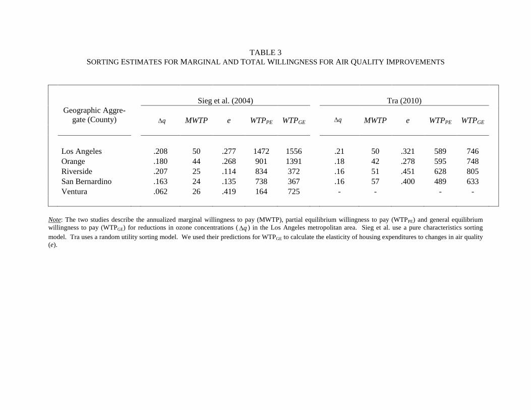
TABLE 3 SORTING ESTIMATES FOR MARGINAL AND TOTAL WILLINGNESS FOR AIR QUALITY IMPROVEMENTS
Sieg et al. (2004)
Tra (2010)
Geographic Aggre-
gate (County)
MWTP e WTPPE WTPGE
MWTP e WTPPE WTPGE
Los Angeles
.208 50 .277 1472 1556
.21 50 .321 589 746
Orange
.180 44 .268 901 1391
.18 42 .278 595 748 Riverside
.207 25 .114 834 372
.16 51 .451 628 805
San Bernardino
.163 24 .135 738 367
.16 57 .400 489 633 Ventura
.062 26 .419 164 725
- -
- -
Note: The two studies describe the annualized marginal willingness to pay (MWTP), partial equilibrium willingness to pay (WTPPE) and general equilibrium willingness to pay (WTPGE) for reductions in ozone concentrations ( q∆ ) in the Los Angeles metropolitan area. Sieg et al. use a pure characteristics sorting model. Tra uses a random utility sorting model. We used their predictions for WTPGE to calculate the elasticity of housing expenditures to changes in air quality (e).
q∆ q∆

P
g jg 1+jg
1+jP
jP 1−iy
1+iy
iy
11 +− << iii yyy
Figure 1. The Single Crossing Condition: Indifference Curves for Three Households Figure 2. Partition of Households across Communities by Income
0 max (y)
j = 1 j = 2 j = J-1 j = J

101
Figure 3. Partition of Households into Communities by Preferences and Income
y
α
j= 3
j=2
3 2 1 g g g < <
3 2 1 p p p < <
j=1

102
1g
( )ghP ,
$2
$1
( )22211 ,,,,| UyhggBid α−
2,1g 1,1g
P
( )11111 ,,,,| UyhggBid α−
Figure 4. Bid Functions for Housing as a Function of 1g in Hedonic Equilibrium
( )hggP ,| 111 −
$
MWTP2
MWTP1
( )11111 ,,,| yhggD α− ( )22112 ,,,| yhggD α−
1g 1,1g 2,1g
Figure 5. Implicit Price Function for 1g and Demand Curves for Two Households

103
APPENDIX TABLE 1 GUIDE TO NOTATION
The Spatial Landscape
Qq ,...,1= Index of housing markets
Locational Characteristics: indexed by the j subscript
Jj ,...,1= Index of locations (depending on the model, j = house, community, or metro area)
h Vector of housing characteristics (e.g. bedrooms, bathrooms, pool)
g Vector of public goods (e.g. air quality, school quality, open space)
[ ]hgx ,⊂ Subset of housing characteristics and public goods observed by the analyst
ξ Vector of characteristics not observed by the analyst
( )hfh = Index of housing characteristics
( )gfg = Index of public goods
( )ξξ f= Index of unobserved characteristics
P Annualized expenditures on a single home
( )ξ,1 xfP = Marginal price function for 1x estimated from a hedonic model
p Annualized “per-unit” price for a homogeneous unit of housing (i.e. the rental rate)
b Composite numeraire private good. Its price is assumed to be normalized to unity
Household Characteristics: indexed by the i subscript
Ii ,...,1= Index of households
wyy += ˆ Total annual income
y Annual exogenous non-wage income
w Annual wage income
( )εα ,df= Preferences for locational characteristics
d Vector of household demographics (e.g. education, age, race, income)
ε Idiosyncratic preferences for locational characteristics
Reduced Form Estimation
Β Parameter vector estimated from the hedonic price function
φ Parameter vector estimated from a capitalization regression
z Instruments for x
Ω Parameter vector estimated from the inverse demand function