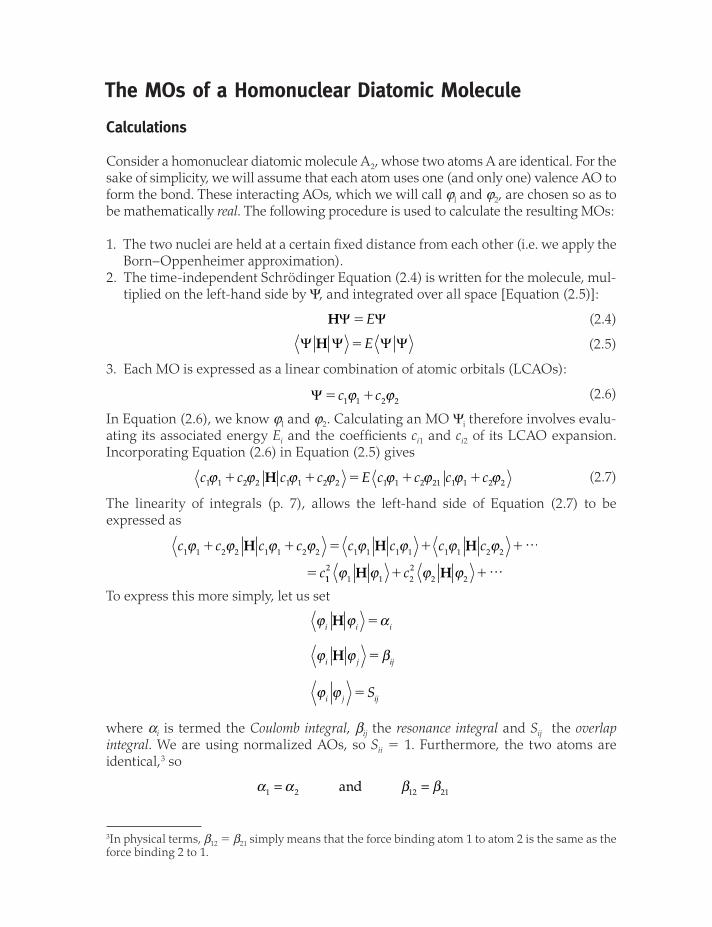
The MOs of a Homonuclear Diatomic Molecule

Calculations

Consider a homonuclear diatomic molecule A2, whose two atoms A are identical. For the sake of simplicity, we will assume that each atom uses one (and only one) valence AO to form the bond. These interacting AOs, which we will call ϕl and ϕ2, are chosen so as to be mathematically real. The following procedure is used to calculate the resulting MOs:

1. The two nuclei are held at a certain fi xed distance from each other (i.e. we apply the Born–Oppenheimer approximation).

2. The time-independent Schrödinger Equation (2.4) is written for the molecule, mul-tiplied on the left-hand side by Ψ, and integrated over all space [Equation (2.5)]:

HΨ Ψ�E (2.4)

Ψ Ψ Ψ ΨH �E (2.5)

3. Each MO is expressed as a linear combination of atomic orbitals (LCAOs):

Ψ � �c c1 1 2 2ϕ ϕ (2.6)

In Equation (2.6), we know ϕl and ϕ2. Calculating an MO Ψi therefore involves evalu-ating its associated energy Ei and the coeffi cients ci1 and ci2 of its LCAO expansion. Incorporating Equation (2.6) in Equation (2.5) gives

c c c c E c c c c1 1 2 2 1 1 2 2 1 1 2 21 1 1 2 2ϕ ϕ ϕ ϕ ϕ ϕ ϕ ϕ� � � � �H (2.7)

The linearity of integrals (p. 7), allows the left-hand side of Equation (2.7) to be expressed as

c c c c c c c c

c

1 1 2 2 1 1 2 2 1 1 1 1 1 1 2 2ϕ ϕ ϕ ϕ ϕ ϕ ϕ� � � � �

�

H H Hϕ …

112

1 1 22

2 2ϕ ϕ ϕ ϕH H� �c …

To express this more simply, let us set

ϕ ϕ α

ϕ ϕ β

ϕ ϕ

i i i

i j ij

i j ijS

H

H

�

�

�

where αi is termed the Coulomb integral, βij the resonance integral and Sij the overlap integral. We are using normalized AOs, so Sii � 1. Furthermore, the two atoms are identical,3 so

α α β β1 2 12 21= =and

3In physical terms, β12 � β21 simply means that the force binding atom 1 to atom 2 is the same as the force binding 2 to 1.

Thus, Equation (2.7) can be written as

( ) ( )c c c c E c c c c S12

22

1 2 12

22

1 22 2 0� � � � � �α β (2.8)

where α, β and S are parameters and c1, c2 and E are unknowns.4. Let us now choose c1 and c2 so as to minimize E (variational method). To do this, we

differentiate Equation (2.8), and set the partial derivatives to zero:

∂∂

∂∂

Ec

Ec1 2

0� �

thus obtaining the secular equations:

( ) ( )

( ) ( )

α ββ α

� � � �

� � � �

E c ES c

ES c E c1 2

1 2

0

0 (2.9)

These equations are homogeneous in ci. They have a nontrivial solution if the secular deter-minant (i.e. the determinant of the coeffi cients of the secular equations) can be set to zero:

α ββ α

α β� �

� �� � � � �

E ES

ES EE ES( ) ( )2 2

0 (2.10)

The solutions to Equation (2.10) are

ES

ES1 2 1

��

��

�

�

α β α β1

and (2.11)

E1 and E2 are the only energies which an electron belonging to the diatomic molecule A2 can have. Each energy level Ei is associated with a molecular orbital Ψi whose coeffi -cients may be obtained by setting E � Ei in Equation (2.9) and solving these equations, taking into account the normalization condition:

Ψ Ψi i i i i ic c c c S� � � �12

22

1 22 1 (2.12)

The solutions are

Ψ Ψ1 1 2 2 1 2

1

2 1

1

2 1�

�� �

��

S S( )( ) ( )

( )ϕ ϕ ϕ ϕand (2.13)

Figure 2.2 gives a pictorial representation of Equation (2.11) and (2.13).

Ψ2

Ψ1

1 2

Figure 2.2 The MOs of the homonuclear diatomic A2. ϕl and ϕ2 are arbitrarily drawn as s orbitals. Note that the destabilization of Ψ2 is greater than the stabilization of Ψ1.

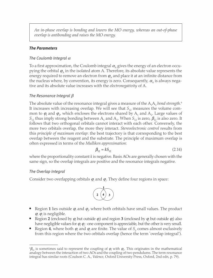
The Parameters

The Coulomb Integral α

To a fi rst approximation, the Coulomb integral αA gives the energy of an electron occu-pying the orbital ϕA in the isolated atom A. Therefore, its absolute value represents the energy required to remove an electron from ϕA and place it at an infi nite distance from the nucleus where, by convention, its energy is zero. Consequently, αA is always nega-tive and its absolute value increases with the electronegativity of A.

The Resonance Integral β

The absolute value of the resonance integral gives a measure of the A1A2 bond strength.6 It increases with increasing overlap. We will see that S12 measures the volume com-mon to ϕl and ϕ2, which encloses the electrons shared by A1 and A2. Large values of S12 thus imply strong bonding between A1 and A2. When S12 is zero, β12 is also zero. It follows that two orthogonal orbitals cannot interact with each other. Conversely, the more two orbitals overlap, the more they interact. Stereoelectronic control results from this principle of maximum overlap: the best trajectory is that corresponding to the best overlap between the reagent and the substrate. The principle of maximum overlap is often expressed in terms of the Mulliken approximation:

β12 12≈ kS (2.14)

where the proportionality constant k is negative. Basis AOs are generally chosen with the same sign, so the overlap integrals are positive and the resonance integrals negative.

The Overlap Integral

Consider two overlapping orbitals ϕi and ϕj. They defi ne four regions in space:

1

2 34

Region 1 lies outside ϕi and ϕj, where both orbitals have small values. The product ϕi ϕj is negligible.Region 2 (enclosed by ϕi but outside ϕj) and region 3 (enclosed by ϕj but outside ϕi) also have negligible values for ϕi ϕj : one component is appreciable, but the other is very small.Region 4, where both ϕi and ϕj are fi nite. The value of Sij comes almost exclusively from this region where the two orbitals overlap (hence the term `overlap integral’).

6β12 is sometimes said to represent the coupling of ϕl with ϕ2. This originates in the mathematical analogy between the interaction of two AOs and the coupling of two pendulums. The term resonance integral has similar roots (Coulson C. A., Valence, Oxford University Press, Oxford, 2nd edn, p. 79).

•

•

•

An in-phase overlap is bonding and lowers the MO energy, whereas an out-of-phase overlap is antibonding and raises the MO energy.

Mulliken Analysis

The MOs in the diatomic molecules discussed above have only two coeffi cients, so their chemical interpretation poses few problems. The situation becomes slightly more complicated when the molecule is polyatomic or when each atom uses more than one AO. Overlap population and net atomic charges can then be used to give a rough idea of the electronic distribution in the molecule.

Overlap Population

Consider an electron occupying Ψ1. Its probability density can best be visualized as a cloud carrying an overall charge of one electron. To obtain the shape of this cloud, we calculate the square of Ψ1:

Ψ Ψ1 1 112

1 1 11 12 12 122

2 22 1� � � �c c c S cϕ ϕ ϕ ϕ (2.15)

Equation (2.15) may be interpreted in the following way. Two portions of the cloud having charges of c11

2 and c122 are essentially localized within the orbitals ϕl and ϕ2

and `belong’ to A1 and A2, respectively. The remainder has a charge of 2c11 2c12S and is concentrated within the zone where the two orbitals overlap. Hence this last portion is termed the overlap population of A1A2. It is positive when the AOs overlap in phase (as in Ψ1) and negative when they are out of phase (as in Ψ2). The overlap population gives the fraction of the electron cloud shared by A1 and A2. A positive overlap popu-lation strengthens a bond, whereas a negative one weakens it. We can therefore take 2c11 c12S as a rough measure7 of the A1A2 bond strength.

Net Atomic Charges

It is often useful to assign a net charge to an atom. This allows the nuclei and electron cloud to be replaced by an ensemble of point charges, from which the dipole moment of the molecule can be easily calculated. It also allows the reactive sites to be identi-fi ed: positively charged atoms will be preferentially attacked by nucleophiles, whereas negatively charged atoms will be favored sites for electrophiles.8

The net charge on an atom is given by the algebraic sum of its nuclear charge qn and its electronic charge qe. The latter is usually evaluated using the Mulliken parti-tion scheme, which provides a simple way of dividing the electron cloud among the atoms of the molecule. Consider an electron occupying the molecular orbital Ψ1 of the diatomic A1A2. The contribution of this electron to the electronic charge of A1 is then c11

2 plus half of the overlap population. In the general case:

q n c c Si i i ji j

e A j AA( ),

�∑ (2.16)

7In a polyelectronic molecule, it is necessary to sum over all electrons and calculate the total overlap population to obtain a measure of the bond strength.8This rule is not inviolable. See pp. 87, 96 and 175.

where SAj is the overlap integral of ϕA and ϕj, ni is the number of electrons which occupy Ψi and ciA and cij are the coeffi cients of ϕA and ϕj in the same MO. The summation takes in all of the MOs Ψi and all of the atoms j in the molecule.

MOs of a Heteronuclear Diatomic Molecule

Calculations

A heteronuclear diatomic molecule is comprised of two different atoms A and B. For simplicity, we will again assume that only one AO on each atom is used to form the bond between A and B. The two relevant AOs are then ϕA, of energy αA and ϕB of energy αB. The calculation is completely analogous to the case of the homonuclear diatomic given above. For a heteronuclear diatomic molecule AB, Equation (2.10) – where the secular determinant is set to zero – becomes

( )( ) ( )α α βA B� � � � �E E ES 2 0 (2.17)

Equation (2.17) is a second-order equation in E which can be solved exactly. However, the analogs of expressions Equation (2.11) and (2.13) are rather unwieldy. For qualita-tive applications, they can be approximated as follows:

E

SE

S1

2

2

2

≈ ≈αβ αα α

αβ αα αA

A

A BB

B

B A

��

��

�

�

( ) ( ) (2.18)

Ψ Ψ1 2≈

⎛

⎝⎜

⎞

⎠⎟ ≈N

SN

S1 2ϕ ϕ ϕ

αAA

A BB

B

B

��

��

�

��

β αα α

β αα AA

ϕ�

⎛

⎝⎜

⎞

⎠⎟ (2.19)

where N1 and N2 are normalization coeffi cients. Equations (2.18) assume that E1 and E2 are not very different from αA and αB, respectively. Using this approximation, it is possible to rewrite Equation (2.17) in the form

αβα

β αα αA

B

A

B A

� ��

�

�

�E

E SE

S1

12

1

2( ) ( )≈ (2.20)

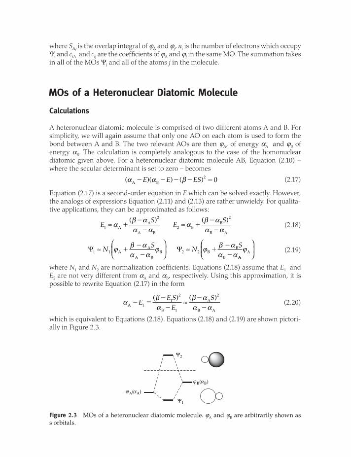
which is equivalent to Equations (2.18). Equations (2.18) and (2.19) are shown pictori-ally in Figure 2.3.

Ψ1

Ψ2

Β( Β)

Α( Α)

Figure 2.3 MOs of a heteronuclear diatomic molecule. ϕA and ϕB are arbitrarily shown as s orbitals.

Huckel Molecular Orbital theory (HMO theory).

An approximate theory that gives us a very quick picture of the MO energy diagram and MO’s of molecules without doing a lot of work.

Structure and bonding in highly conjugated systems nicely treated by

HMO. Look at examples:

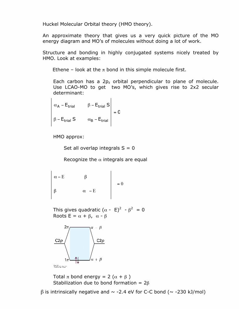
Ethene – look at the π bond in this simple molecule first.

Each carbon has a 2pz orbital perpendicular to plane of molecule. Use LCAO-MO to get two MO’s, which gives rise to 2x2 secular determinant:

HMO approx: Set all overlap integrals S = 0 Recognize the α integrals are equal

This gives quadratic (α - E)2 - β2 = 0 Roots E = α + β, α - β

Total π bond energy = 2 (α + β ) Stabilization due to bond formation = 2β

β is intrinsically negative and ~ -2.4 eV for C-C bond (~ -230 kJ/mol)

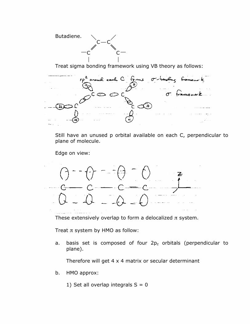
Butadiene.

Treat sigma bonding framework using VB theory as follows:

Still have an unused p orbital available on each C, perpendicular to

plane of molecule.

Edge on view:

These extensively overlap to form a delocalized π system.

Treat π system by HMO as follow: a. basis set is composed of four 2pz orbitals (perpendicular to

plane). Therefore will get 4 x 4 matrix or secular determinant b. HMO approx: 1) Set all overlap integrals S = 0

C C

C C

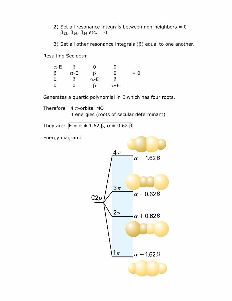
2) Set all resonance integrals between non-neighbors = 0 β13, β14, β24 etc. = 0 3) Set all other resonance integrals (β) equal to one another. Resulting Sec detm α-E β 0 0 β α-E β 0 = 0 0 β α-E β 0 0 β α–E Generates a quartic polynomial in E which has four roots. Therefore 4 π-orbital MO 4 energies (roots of secular determinant) They are: E = α ± 1.62 β, α ± 0.62 β Energy diagram:

31

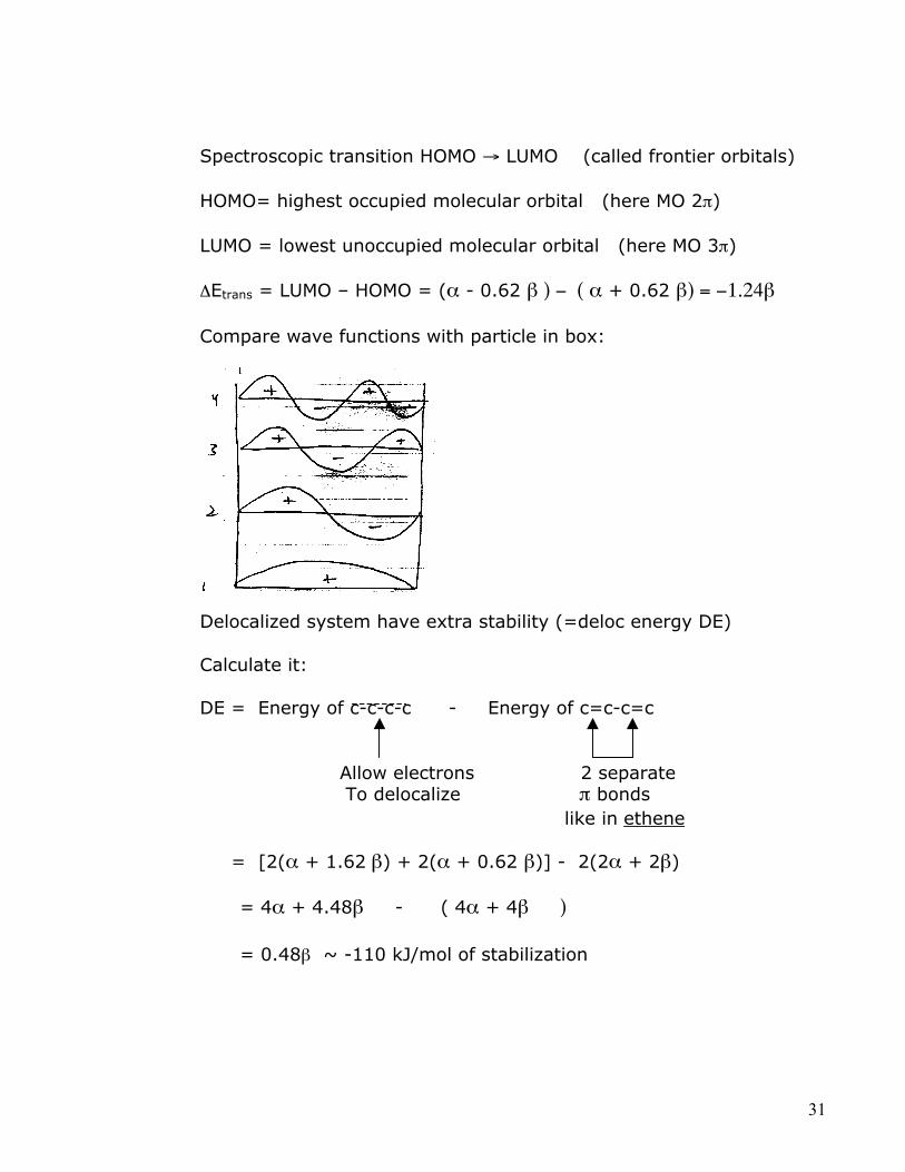
Spectroscopic transition HOMO → LUMO (called frontier orbitals) HOMO= highest occupied molecular orbital (here MO 2π) LUMO = lowest unoccupied molecular orbital (here MO 3π) ΔEtrans = LUMO – HOMO = (α - 0.62 β ) − ( α + 0.62 β) = −1.24β Compare wave functions with particle in box:

Delocalized system have extra stability (=deloc energy DE) Calculate it: DE = Energy of c-c-c-c - Energy of c=c-c=c Allow electrons 2 separate To delocalize π bonds like in ethene = [2(α + 1.62 β) + 2(α + 0.62 β)] - 2(2α + 2β) = 4α + 4.48β - ( 4α + 4β ) = 0.48β ~ -110 kJ/mol of stabilization

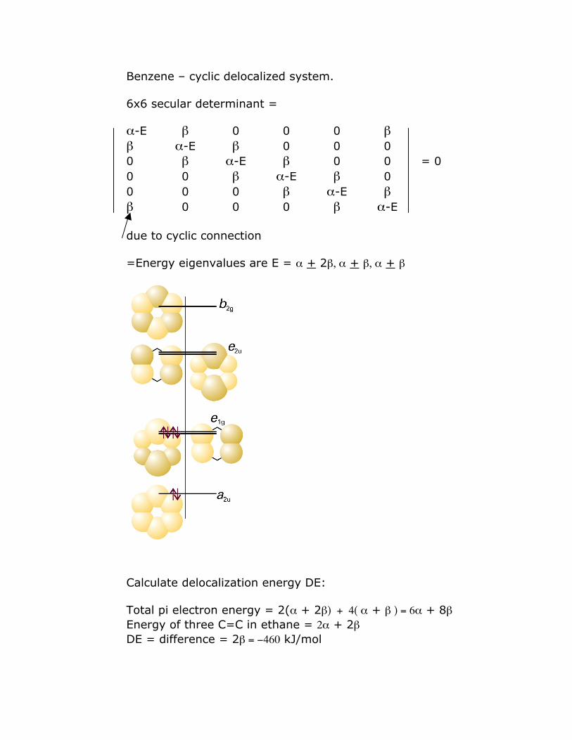
Benzene – cyclic delocalized system. 6x6 secular determinant = α-E β 0 0 0 β β α-E β 0 0 0 0 β α-E β 0 0 = 0 0 0 β α-E β 0 0 0 0 β α-E β β 0 0 0 β α-E due to cyclic connection

=Energy eigenvalues are E = α + 2β, α + β, α + β

Calculate delocalization energy DE: Total pi electron energy = 2(α + 2β) + 4( α + β ) = 6α + 8β Energy of three C=C in ethane = 2α + 2β DE = difference = 2β = −460 kJ/mol

General Reviews

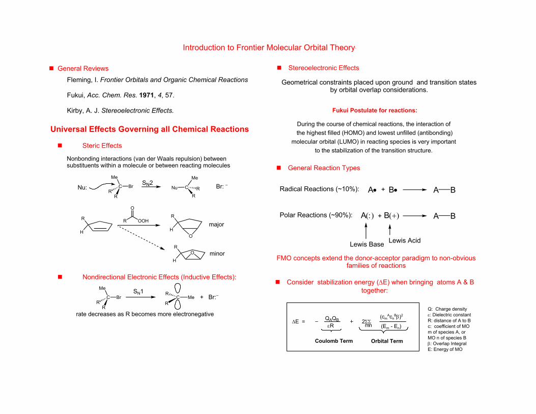
Introduction to Frontier Molecular Orbital Theory-

Fleming, I. Frontier Orbitals and Organic Chemical Reactions

Fukui, Acc. Chem. Res. 1971, 4, 57.

Kirby, A. J. Stereoelectronic Effects.

+ Br:–

minor

major

Br: –Nu:

During the course of chemical reactions, the interaction of the highest filled (HOMO) and lowest unfilled (antibonding)

molecular orbital (LUMO) in reacting species is very important to the stabilization of the transition structure.

Geometrical constraints placed upon ground and transition statesby orbital overlap considerations.

Stereoelectronic Effects

Nonbonding interactions (van der Waals repulsion) between substituents within a molecule or between reacting molecules

Steric Effects

Universal Effects Governing all Chemical Reactions

Nondirectional Electronic Effects (Inductive Effects):

SN1

rate decreases as R becomes more electronegative

C Br

Me

RR

C RR

Me

Nu

R

H

R OOH

O

OH

R

R

HO

CR

R

Me

Br C MeR

R

Fukui Postulate for reactions:

SN2

General Reaction Types

Radical Reactions (~10%): A• B•+ A B

Polar Reactions (~90%): A(:) B(+)+ A B

Lewis Base Lewis Acid

FMO concepts extend the donor-acceptor paradigm to non-obvious families of reactions

QAQB

Q: Charge densityε: Dielectric constantR: distance of A to Bc: coefficient of MO m of species A, or MO n of species Bβ: Overlap IntegralE: Energy of MO

∆E =(cm

AcnBβ)2

(Em - En)mnεR

Coulomb Term Orbital Term

Consider stabilization energy (∆E) when bringing atoms A & B together:

2ΣΣ

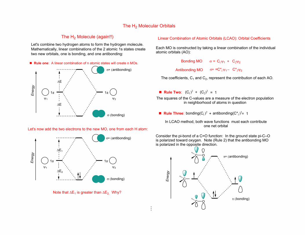
The H2 Molecule (again!!)Let's combine two hydrogen atoms to form the hydrogen molecule.Mathematically, linear combinations of the 2 atomic 1s states createtwo new orbitals, one is bonding, and one antibonding:

Ener

gy

1s 1s

σ∗ (antibonding)

Rule one: A linear combination of n atomic states will create n MOs.

∆E

∆E

Let's now add the two electrons to the new MO, one from each H atom:

Note that ∆E1 is greater than ∆E2. Why?

σ (bonding)

σ (bonding)

∆E2

∆E1

σ∗ (antibonding)

1s1s

ψ2

ψ2

ψ1

ψ1

Ener

gy

+C1ψ1σ = C2ψ2

Linear Combination of Atomic Orbitals (LCAO): Orbital Coefficients

Each MO is constructed by taking a linear combination of the individual atomic orbitals (AO):

Bonding MO

Antibonding MO C*2ψ2σ∗ =C*1ψ1–

The coefficients, C1 and C2, represent the contribution of each AO.

Rule Two: (C1)2 + (C2)2 = 1

= 1antibonding(C*1)2+bonding(C1)2 Rule Three:

Ener

gy

π∗ (antibonding)

π (bonding)

Consider the pi-bond of a C=O function: In the ground state pi-C–Ois polarized toward oxygen. Note (Rule 2) that the antibonding MOis polarized in the opposite direction.

C

C

O

C O

The H2 Molecular Orbitals

The squares of the C-values are a measure of the electron populationin neighborhood of atoms in question

In LCAO method, both wave functions must each contribute one net orbital

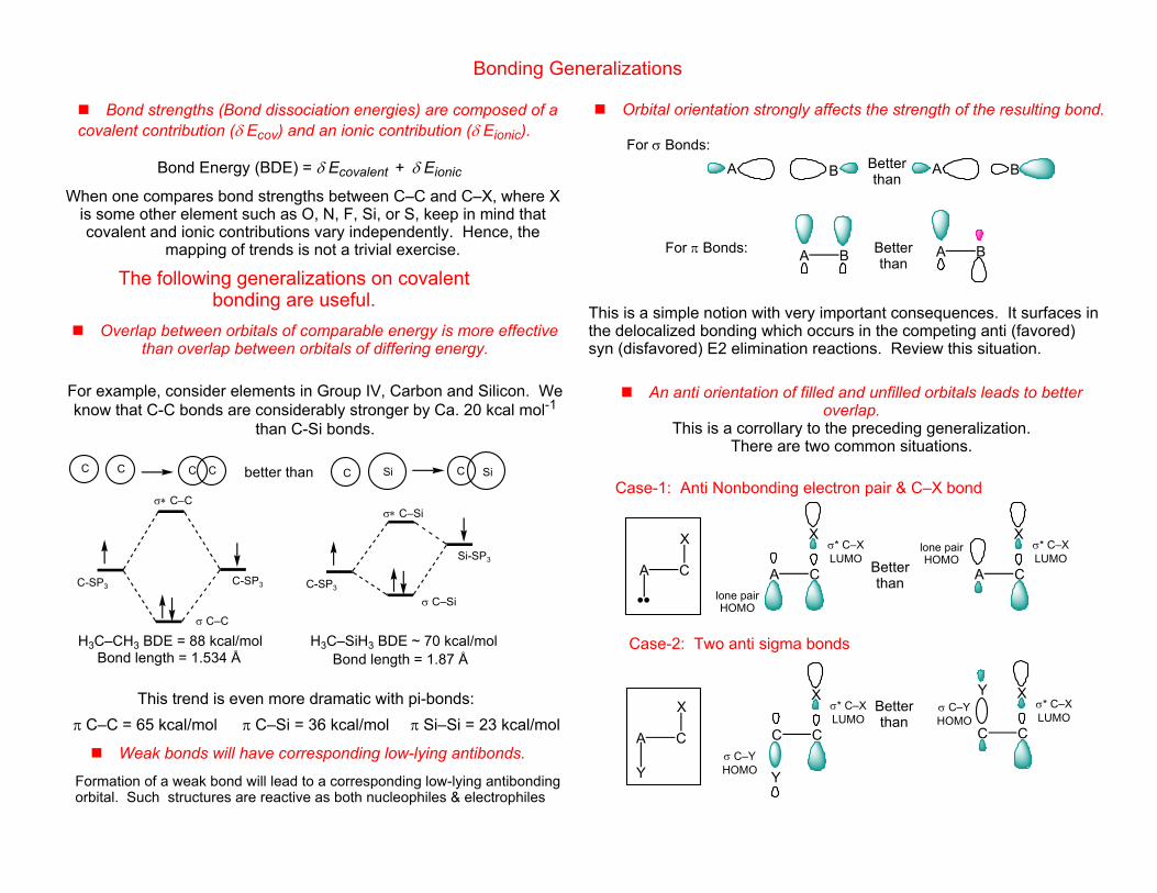
Bonding Generalizations

Weak bonds will have corresponding low-lying antibonds.

π Si–Si = 23 kcal/molπ C–Si = 36 kcal/molπ C–C = 65 kcal/molThis trend is even more dramatic with pi-bonds:

σ∗ C–Siσ∗ C–C

σ C–Si

σ C–C

Bond length = 1.87 ÅBond length = 1.534 ÅH3C–SiH3 BDE ~ 70 kcal/molH3C–CH3 BDE = 88 kcal/mol

The following generalizations on covalent bonding are useful.

When one compares bond strengths between C–C and C–X, where X is some other element such as O, N, F, Si, or S, keep in mind that covalent and ionic contributions vary independently. Hence, the

mapping of trends is not a trivial exercise.

Bond Energy (BDE) = δ Ecovalent + δ Eionic

Bond strengths (Bond dissociation energies) are composed of a covalent contribution (δ Ecov) and an ionic contribution (δ Eionic).

better than

For example, consider elements in Group IV, Carbon and Silicon. We know that C-C bonds are considerably stronger by Ca. 20 kcal mol-1

than C-Si bonds.

Overlap between orbitals of comparable energy is more effective than overlap between orbitals of differing energy.

Formation of a weak bond will lead to a corresponding low-lying antibonding orbital. Such structures are reactive as both nucleophiles & electrophiles

••

Better than

Better than

Case-2: Two anti sigma bonds

σ C–YHOMO

σ* C–XLUMO

σ* C–XLUMO

lone pairHOMO

σ* C–XLUMO

σ* C–XLUMO

lone pairHOMO

Case-1: Anti Nonbonding electron pair & C–X bond

An anti orientation of filled and unfilled orbitals leads to better overlap.

This is a corrollary to the preceding generalization. There are two common situations.

Better than

For π Bonds:

For σ Bonds:

Orbital orientation strongly affects the strength of the resulting bond.

Better than

This is a simple notion with very important consequences. It surfaces inthe delocalized bonding which occurs in the competing anti (favored) syn (disfavored) E2 elimination reactions. Review this situation.

σ C–YHOMO

A C A C

C CC C

A C

X

A

Y

C

X

A B A B

C-SP3

Si-SP3

C-SP3C-SP3

SiC Si CCCCC

Y

Y

X X

XX

BABA

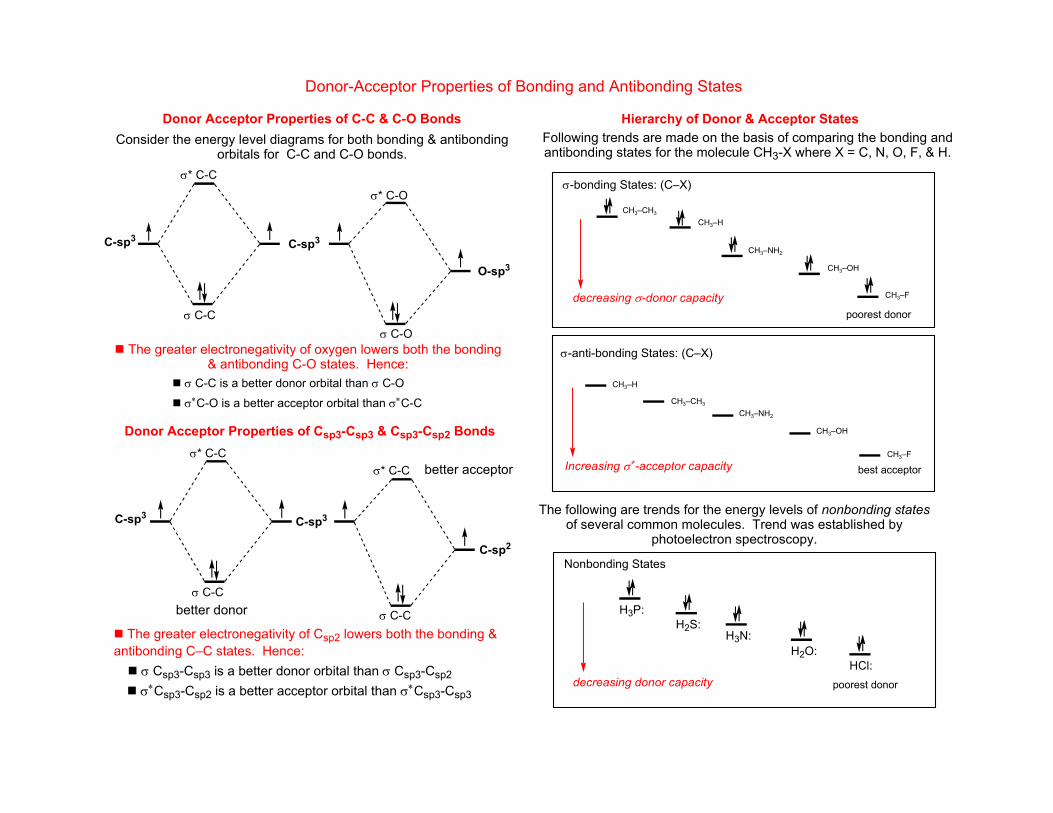
Donor-Acceptor Properties of Bonding and Antibonding States

σ∗Csp3-Csp2 is a better acceptor orbital than σ∗Csp3-Csp3

C-sp3

C-sp3

σ* C-C

σ C-C

C-sp3

σ C-C

σ* C-C

C-sp2

Donor Acceptor Properties of Csp3-Csp3 & Csp3-Csp2 Bonds

The greater electronegativity of Csp2 lowers both the bonding & antibonding C–C states. Hence:

σ Csp3-Csp3 is a better donor orbital than σ Csp3-Csp2

σ∗C-O is a better acceptor orbital than σ∗C-C

σ C-C is a better donor orbital than σ C-O

The greater electronegativity of oxygen lowers both the bonding & antibonding C-O states. Hence:

Consider the energy level diagrams for both bonding & antibonding orbitals for C-C and C-O bonds.

Donor Acceptor Properties of C-C & C-O Bonds

O-sp3

σ* C-O

σ C-O

C-sp3

σ C-C

σ* C-C

better donor

better acceptor

decreasing donor capacity

Nonbonding States

poorest donor

The following are trends for the energy levels of nonbonding states of several common molecules. Trend was established by

photoelectron spectroscopy.

best acceptor

poorest donor

Increasing σ∗-acceptor capacity

σ-anti-bonding States: (C–X)

σ-bonding States: (C–X)

decreasing σ-donor capacity

Following trends are made on the basis of comparing the bonding and antibonding states for the molecule CH3-X where X = C, N, O, F, & H.

Hierarchy of Donor & Acceptor States

CH3–CH3

CH3–H

CH3–NH2

CH3–OH

CH3–F

CH3–H

CH3–CH3

CH3–NH2

CH3–OH

CH3–F

HCl:H2O:

H3N:H2S:

H3P:

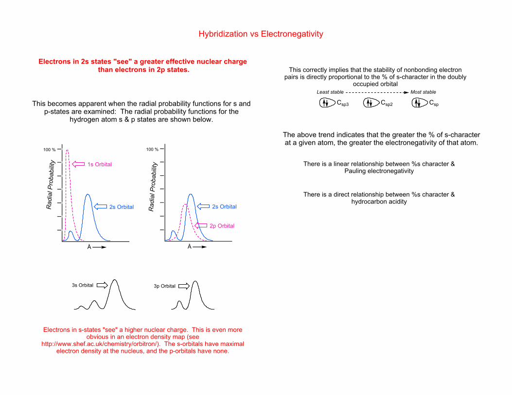
3p Orbital

This becomes apparent when the radial probability functions for s and p-states are examined: The radial probability functions for the

hydrogen atom s & p states are shown below.

3s Orbital

Electrons in 2s states "see" a greater effective nuclear charge than electrons in 2p states. This correctly implies that the stability of nonbonding electron

pairs is directly proportional to the % of s-character in the doubly occupied orbital

Least stable Most stable

The above trend indicates that the greater the % of s-character at a given atom, the greater the electronegativity of that atom.

There is a direct relationship between %s character & hydrocarbon acidity

There is a linear relationship between %s character & Pauling electronegativity

Hybridization vs Electronegativity

Å

Rad

ial P

roba

bilit

y100 %

2p Orbital

2s Orbital2s Orbital

1s Orbital

100 %

Rad

ial P

roba

bilit

y

Å

Electrons in s-states "see" a higher nuclear charge. This is even more obvious in an electron density map (see

http://www.shef.ac.uk/chemistry/orbitron/). The s-orbitals have maximal electron density at the nucleus, and the p-orbitals have none.

Csp3 Csp2 Csp

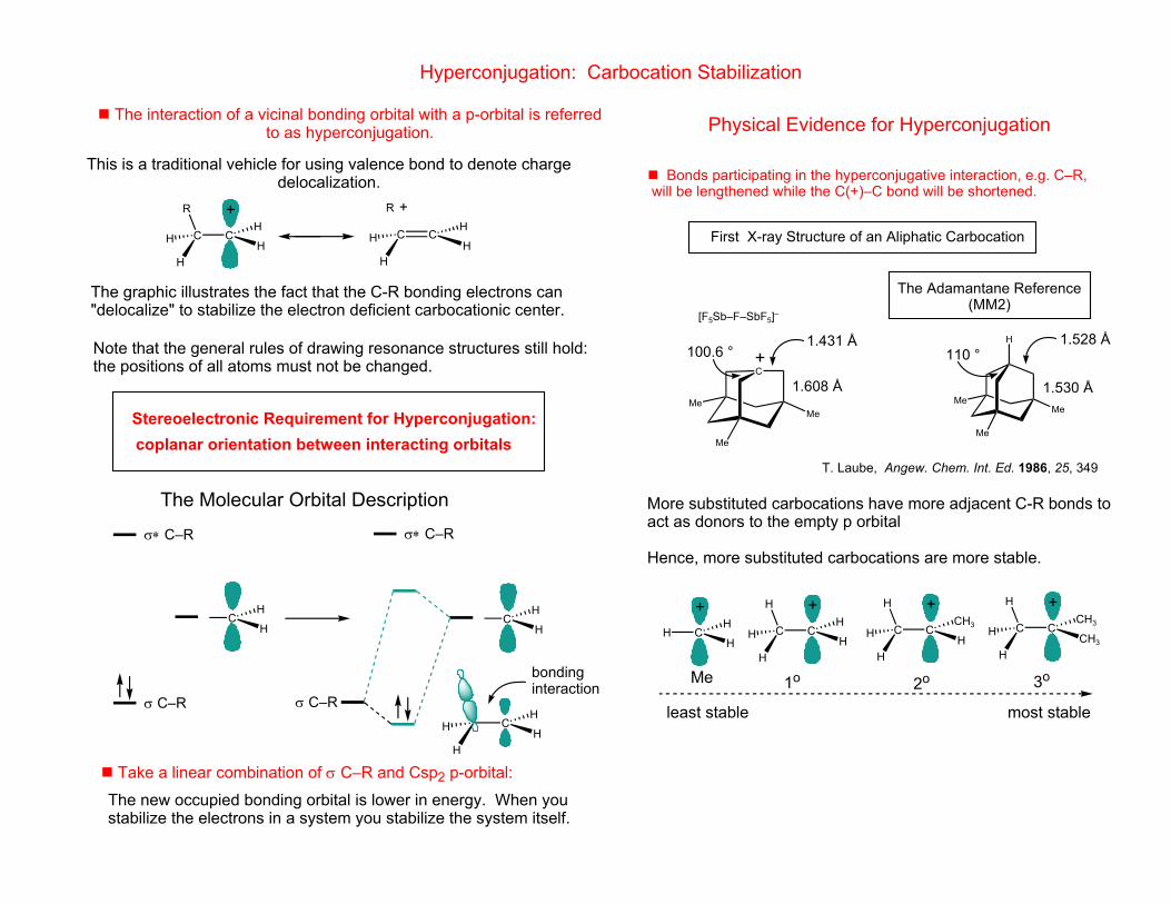
[F5Sb–F–SbF5]–

The Adamantane Reference(MM2)

T. Laube, Angew. Chem. Int. Ed. 1986, 25, 349

First X-ray Structure of an Aliphatic Carbocation

110 °100.6 °

1.530 Å1.608 Å

1.528 Å1.431 Å

Bonds participating in the hyperconjugative interaction, e.g. C–R, will be lengthened while the C(+)–C bond will be shortened.

Physical Evidence for Hyperconjugation

The new occupied bonding orbital is lower in energy. When you stabilize the electrons in a system you stabilize the system itself.

Take a linear combination of σ C–R and Csp2 p-orbital:

σ C–R

σ∗ C–R

σ C–R

σ∗ C–R

The Molecular Orbital Description

coplanar orientation between interacting orbitalsStereoelectronic Requirement for Hyperconjugation:

The graphic illustrates the fact that the C-R bonding electrons can "delocalize" to stabilize the electron deficient carbocationic center.

Note that the general rules of drawing resonance structures still hold:the positions of all atoms must not be changed.

+

The interaction of a vicinal bonding orbital with a p-orbital is referred to as hyperconjugation.

Hyperconjugation: Carbocation Stabilization

Me

Me

Me

H

C C

R

H

H H

HC

H

HCH

H

CH

HC

H

H

Me

Me

Me

C

R

This is a traditional vehicle for using valence bond to denote charge delocalization.

+

+

C

H

H H

H

bonding interaction

More substituted carbocations have more adjacent C-R bonds to act as donors to the empty p orbital

Hence, more substituted carbocations are more stable.

C C

H

H

H H

H+

H CH

H+

C C

H

H

H H

CH3

+C C

H

H

H CH3

CH3

+

least stable most stable

Me 1o 2o 3o

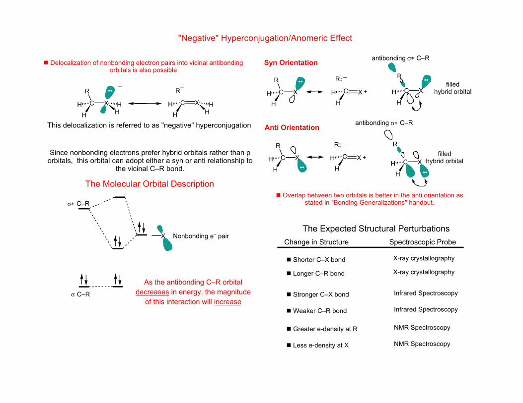
NMR Spectroscopy Greater e-density at R

Less e-density at X NMR Spectroscopy

Longer C–R bond X-ray crystallography

Infrared Spectroscopy Weaker C–R bond

Stronger C–X bond Infrared Spectroscopy

X-ray crystallography Shorter C–X bond

Spectroscopic ProbeChange in Structure

The Expected Structural Perturbations

As the antibonding C–R orbital decreases in energy, the magnitude

of this interaction will increase σ C–R

σ∗ C–R

The Molecular Orbital Description

Delocalization of nonbonding electron pairs into vicinal antibonding orbitals is also possible

"Negative" Hyperconjugation/Anomeric Effect

X

Since nonbonding electrons prefer hybrid orbitals rather than p orbitals, this orbital can adopt either a syn or anti relationship to

the vicinal C–R bond.

C X

R

HH

HH X H

HCH

H

R–

This delocalization is referred to as "negative" hyperconjugation antibonding σ∗ C–R

Overlap between two orbitals is better in the anti orientation as stated in "Bonding Generalizations" handout.

+

–

Anti Orientation

filled hybrid orbital

filled hybrid orbital

antibonding σ∗ C–RSyn Orientation

–

+C X

HH

C X

HHCH

CHH

R

X

H

R

XC X

HH

C X

HH

R:

R:

Nonbonding e– pair

–

R

R

We now conclude that this is another example of negative hyperconjugation.

The Anomeric Effect and Related Issues

filled N-sp2

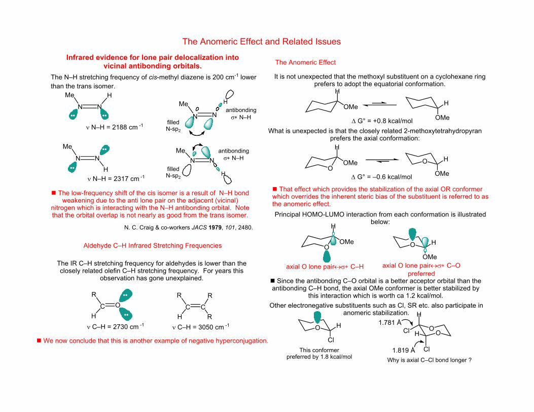
The low-frequency shift of the cis isomer is a result of N–H bond weakening due to the anti lone pair on the adjacent (vicinal)

nitrogen which is interacting with the N–H antibonding orbital. Note that the orbital overlap is not nearly as good from the trans isomer.

Infrared evidence for lone pair delocalization into vicinal antibonding orbitals.

ν N–H = 2188 cm -1

ν N–H = 2317 cm -1

filled N-sp2

antibonding σ∗ N–H

antibonding σ∗ N–H

The N–H stretching frequency of cis-methyl diazene is 200 cm-1 lower than the trans isomer.

N. C. Craig & co-workers JACS 1979, 101, 2480.

ν C–H = 3050 cm -1ν C–H = 2730 cm -1

Aldehyde C–H Infrared Stretching Frequencies

The IR C–H stretching frequency for aldehydes is lower than the closely related olefin C–H stretching frequency. For years this

observation has gone unexplained.

The Anomeric Effect

It is not unexpected that the methoxyl substituent on a cyclohexane ring prefers to adopt the equatorial conformation.

∆ G° = +0.8 kcal/mol

∆ G° = –0.6 kcal/mol

What is unexpected is that the closely related 2-methoxytetrahydropyranprefers the axial conformation:

That effect which provides the stabilization of the axial OR conformerwhich overrides the inherent steric bias of the substituent is referred to asthe anomeric effect.

axial O lone pair↔σ∗ C–H axial O lone pair↔σ∗ C–Opreferred

Principal HOMO-LUMO interaction from each conformation is illustrated below:

Since the antibonding C–O orbital is a better acceptor orbital than the antibonding C–H bond, the axial OMe conformer is better stabilized by

this interaction which is worth ca 1.2 kcal/mol.Other electronegative substituents such as Cl, SR etc. also participate in

anomeric stabilization.

This conformer preferred by 1.8 kcal/mol

1.819 Å

1.781 Å

Why is axial C–Cl bond longer ?

N N

Me H

N

H

N

Me

CH

C

RO

HC

R R

R

N NMe

H

OMe H

OMe

OMe

H

N N

Me

OMe

H

OO

O

H

OMe O H

OMe

Cl

HO O O

H

Cl H

Cl

H

H

E

E

EE

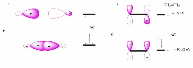
CH2=CH2

+1.5 eV

–10.52 eV

+– –

––

– –

–

–

+

++

+

+

++

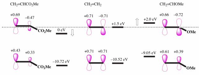
OMe

OMe

CO2Me

CO2Me 0 eV

–10.72 eV

+0.71 –0.71

+0.71 +0.71

+0.66

+0.61

+1.5 eV+2.0 eV

–10.52 eV–9.05 eV

CH2=CHOMe

+0.39

–0.72+0.69–0.47

+0.43 +0.33

CH2=CH2CH2=CHCO2Me

HOMO and LUMO Energies and Orbital Coefficients of Common Alkenes

X X

LUMO

c1 c2 c3 c4

HOMO

Alkene HOMO (eV) c1 c2 LUMO (eV) c3 c4

CH2=CH2a –10.52 0.71 0.71 +1.5 0.71 –0.71

CH2=CHCla –10.15 0.44 0.30 +0.5 0.67 –0.54

CH2=CHMea –9.88 0.67 0.56 +1.8a,b 0.67 –0.65

MeCH=CHMe –9.13c +2.22d

EtCH=CH2 –9.63e +2.01e

–8.94f,g +2.1g

CH2=CHOMea –9.05;–8.93c 0.61 0.39 +2.0 0.66 –0.72

CH2=CHSMea –8.45 0.34 0.17 +1.0 0.63 –0.48

CH2=CHNMe2a –9.0 0.50 0.20 +2.5 0.62 –0.69

CH2=CHCO2Me –10.72 0.43 0.33 0 0.69 –0.47

CH2=CHCN –10.92 0.60 0.49 0 0.66 –0.54

CH2=CHNO2a –11.4 0.62 0.60 +0.7 0.54 –0.32

CH2=CHPh –8.48 0.49 0.32 +0.8 0.48 –0.33

CH2=CHCHO –10.89b 0.58a 0.48a +0.60b 0.404b –0.581b

CH2=CHCHO/BF3b –12.49 +0.43 0.253 –0.529

CH2=CHCO2Hb –10.93 +2.91 0.461 –0.631

O O

–10.29h –1.91i

Ph

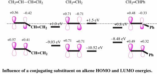
PhCH=CH2

CH=CH2

–0.42

CH2=CH2CH2=CH—CH=CH2

+0.41 –9.03 eV+0.57

+0.56 +0.71 –0.71

+0.71 +0.71

+0.48

+0.49

+1.5 eV+0.8 eV

–10.52 eV

–8.48 eV +0.32

–0.33

CH2=CHPh

+1.0 eV

Influence of a conjugating substituent on alkene HOMO and LUMO energies.

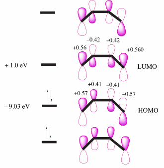
+ 1.0 eV

HOMO

LUMO

+0.560–0.42

–0.57–0.41+0.41

+0.57

–0.42+0.56

– 9.03 eV

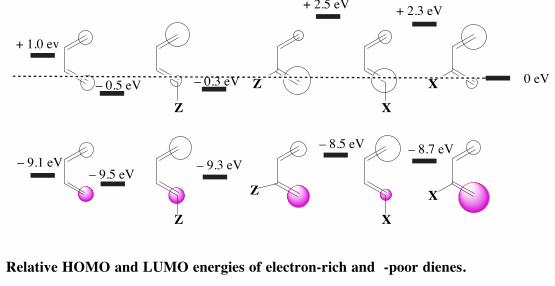
Z

Z

Z

Z

X

X

X

X

– 8.7 eV

0 eV

+ 2.3 eV

– 8.5 eV– 9.3 eV

– 9.5 eV

+ 2.5 eV

– 0.3 eV– 0.5 eV

– 9.1 eV

+ 1.0 ev

Relative HOMO and LUMO energies of electron-rich and -poor dienes.

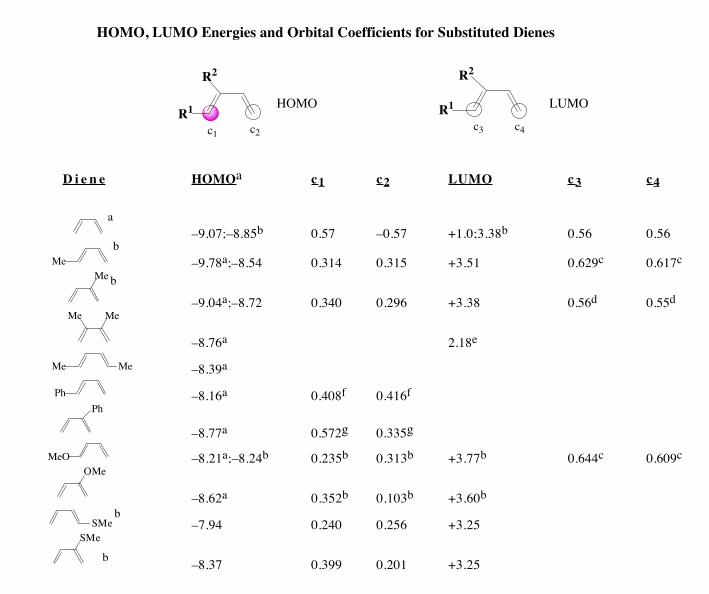
HOMO, LUMO Energies and Orbital Coefficients for Substituted Dienes

R1 R1

R2R2

c4c2c1

LUMOHOMO

c3

D i e n e HOMOa c1 c2 LUMO c3 c4

a

–9.07;–8.85b 0.57 –0.57 +1.0;3.38b 0.56 0.56

Meb

–9.78a;–8.54 0.314 0.315 +3.51 0.629c 0.617c

Me b

–9.04a;–8.72 0.340 0.296 +3.38 0.56d 0.55d

Me Me

–8.76a 2.18e

Me Me –8.39a

Ph –8.16a 0.408f 0.416f

Ph

–8.77a 0.572g 0.335g

MeO –8.21a;–8.24b 0.235b 0.313b +3.77b 0.644c 0.609c

OMe

–8.62a 0.352b 0.103b +3.60b

SMeb

–7.94 0.240 0.256 +3.25

SMe

b –8.37 0.399 0.201 +3.25

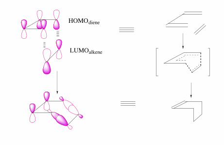
LUMOalkene

HOMOdiene

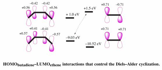
+0.71

–0.71+0.71+1.5 eV

–10.52 eV

+0.56–0.42

+0.57+0.41 –0.41

–0.57

–0.42+0.56

+ 1.0 eV

–9.03 eV

+0.71

HOMObutadiene–LUMOethene interactions that control the Diels–Alder cyclization.

–9.05 eV

–10.72 eV–10.52 eV

+2.0 eV

0 eV

+1.5 eV

+1.0 eV

–9.07 eV

E = 11.07 eV

E = 10.57 eV

E = 9.07 eV

MeOEtO2C

HOMOdiene–LUMOalkene interactions of butadiene and representative alkenes

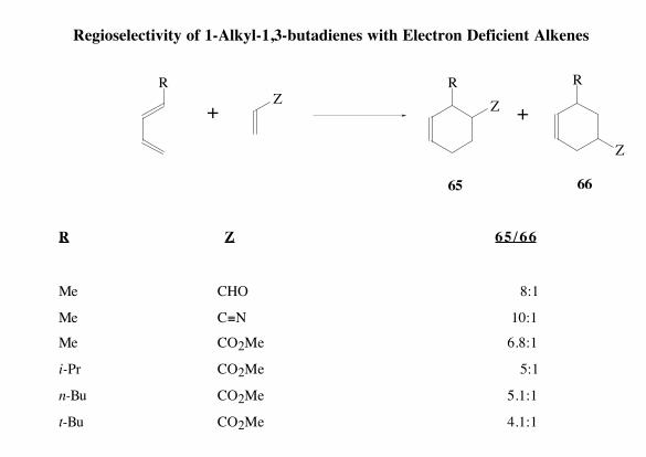
Regioselectivity of 1-Alkyl-1,3-butadienes with Electron Deficient Alkenes

ZR R

Z

R

Z

+ +

65 66

R Z 6 5 / 6 6

Me CHO 8:1

Me C N 10:1

Me CO2Me 6.8:1

i-Pr CO2Me 5:1

n-Bu CO2Me 5.1:1

t-Bu CO2Me 4.1:1

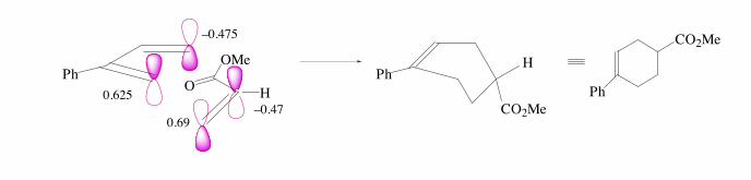
CO2Me

HPh

Ph

CO2Me

H

–0.475

0.625–0.47

0.69

O

OMePh