Embed Size (px)
DESCRIPTION
This review presents in a comprehensive and tutorial form the basic principles of the Monte Carlo method, as applied to the solution of transport problems in semiconductors. Sufficient details of a typical Monte Carlo simulation have been given to allow the interested reader to create his own Monte Carlo program, and the method has been briefly compared with alternative theoretical techniques. Applications have been limited to the case of covalent semiconductors. Particular attention has been paid to the evaluation of the integrated scattering probabilities, for which final expressions are given in a form suitable for their direct use. A collection of results obtained with Monte Carlo simulations is presented, with the aim of showing the power of the method in obtaining physical insights into the processes under investigation. Special technical aspects of the method and updated microscopic models have been treated in some appendixes.
Citation preview

The Monte Carlo method for the solution of charge transportin semiconductors with applications to covalent materials
Carlo Jacoboni and Lino Reggiani
Gruppo Nazionale di Struttura della Materia, Istituto di Fisica dell'Universita di Modena, Via Carnpi 213/A, 41100Modena Italy
This review presents in a comprehensive and tutorial form the basic principles of the Monte Carlo method,as applied to the solution of transport problems in semiconductors. Sufficient details of a typical MonteCarlo simulation have been given to allow the interested reader to create his own Monte Carlo program,and the method has been briefly compared with alternative theoretical techniques. Applications have beenlimited to the case of covalent semiconductors. Particular attention has been paid to the evaluation of theintegrated scattering probabilities, for which final expressions are given in a form suitable for their directuse. A collection of results obtained with Monte Carlo simulations is presented, with the aim of showingthe power of the method in obtaining physical insights into the processes under investigation. Specialtechnical aspects of the method and updated microscopic models have been treated in some appendixes.
CONTENTS
List of SymbolsI. Introduction
II. The Monte Carlo MethodA. FundamentalsB. A typical Monte Carlo program
1. Definition of the physical system2. Initial conditions of motion3. Flight duration —self-scattering4. Choice of the scattering mechanism5. Choice of the state after scattering6. Collection of results for steady-state phenomena
a. Time averagesb. Synchronous ensemble
c. Statistical uncertaintyC. Time- and space-dependent phenomena
1. Transients2. Space-dependent phenomena3. Periodic fields
D. Diffusion1. Fick diffusion2. Velocity autocorrelation function3. Diffusion at small distances and short times; q-
and co-dependent diffusion4. Noise and diffusion
E. Ohmic mobilityF. Impact ionizationG. Magnetic fieldsH. Electron-electron interaction
1. Electron-electron collisions2. Degenerate statistics
I. Variance-reducing techniques1. Variance due to thermal fluctuations2. Variance due to valley repopulation3. Variance related to improbable electron states
J. Survey of other techniques1. Analytical techniques2. Other numerical techniques —the iterative tech-
nique3. A critical comparison of the different techniques
III. Application to covalent semiconductors —microscopicmodelA. Band structure
1. Relationship of energy to wave vector2. Nonparabolicity3. Herring and Vogt transformation
B. Actual bands of covalent semiconductors1. Conduction band
646647648648649649649650652653653653653654655655655656656657658
658659659660660661661662662662663663663663
664666
667667667668669669670
a. Siliconb. Germaniumc. Diamond
2. Valence bandC. Scattering mechanisms in covalent semiconductors
1. Classification2. Fundamentals of scattering
a. General theoryb. Overlap factor
D. Scattering probabilities1. Phonon scattering
a. Electron intravalley scattering —acoustic pho-nons
b. Electron intravalley scattering —optical pho-nons
c. Electron intervalley scatteringd. Hole intraband scattering —acoustic phononse. Hole intraband scattering —optical phononsf. Hole interband scattering
g. Selection rules
2. Ionized impurity scatteringa. Electronsb. Holes
3. Carrier-carrier interaction4. Relative importance of the different scattering
mechanismsIV. Applications to Covalent Semiconductors —Results
A. The simple modelB. Real-model applications
1. Drift velocity2. Ohmic mobility3. Diffusion4. Mean energy5. Distribution function6. Repopulation7. Energy relaxation time8. Efficiency of scattering mechanisms9. White noise
10. Velocity autocorrelation function11. Alternating electric fields12. Magnetic fields13. Transients
C. DevicesV. Conclusions
Acknowledgments
Appendix A: Generation of Random Numbers1. Generation of evenly distributed random numbers
2. Generation of random numbers with given distribu-tions
670670670670670670671671672672672
673
677678F19680680680681682683684
684685685686686688689690691691692692693694695695696696697697697697
698
Reviews of Modern Physics, Vol. 55, No. 3, July 1983 Copyright 1983 The American Physical Society 645

C. Jacoboni and L. Reggiani: Monte Carlo method in transport
698698699699
699
700701703
LIST OF SYMBOI S
aoQq, aq
b
BBC
[c)Cc(t)
dp
DDs
eggi
gpE
EHf(k)
H'
kk, b
lattice parameterphonon annihilation and creation operatorsinverse valence-band parameterimpact parameter for ionized impurityscat teringmagnetic fieldinverse valence-band parametervelocity of lightcrystal statesinverse valence-band parameterautocorrelation function of velocityfluctuationsdeformation potential constant for holeoptical-phonon interactiondiffusion coefficientdiffusion coefficient longitudinal withrespect to the field directiondiffusion coefficient transverse withrespect to the field directiondeformation potential constant for opticaland intervalley-phonon scattering withelectronsunit charge with its signdeformation potential tensorelectron acoustic-phonon deformationpotentialhole acoustic-phonon deformation potentialelectric fieldcomponent of the electric field parallel tothe drift velocitya critical field used in connection withquasielastic approximationHall component of the electric fieldcarrier distribution function in momentumspacecarrier distribution in energy space ofcold and hot valleyselectron-hole pair generation rate perparticle per unit timeoverlap factorreciprocal lattice vectorPlanck constant divided by 2m.
Fourier transform of the perturbationHamiltonianperturbation Hamiltonian for scattering ofelectronscurrent densitywave vector of a carrierk state after and before scattering
a. Direct techniqueb. Rejection techniquec. Combined techniqued. Discrete case
Appendix 8; Nonparabolicity Parameter for Si-like ConductionBand
Appendix C: Parameters for Diamond, Silicon, and Germani-Um
Appendix D: Numerical Evaluation of Integrals of InterestReferences
KgK21
l,p
m,mdmh
mI,
mpmI-
M
n(k)n (r)n, b(k)
n, h
nrn&
n~
npX
pH(k, t)dt
2~'(x, t)
P(k)P(k, k')
P;(k)
P„(cos9)P, „(~)P,, , (e)
P, ,p(~)Pt, „(e)
Ph, (e)Pc,h;h, c
average wave vector of a driftedMaxwellian distribution functionlongitudinal and transverse electron wave-vector component for an ellipsoidalequienergetic surfaceinitial value of kBoltzmann constantmodified Bessel function of order 2carrier mean free patha mean free path for optical-phononinteractioneffective massconductivity effective massdensity-of-states effective massdensity-of-states effective mass of heavyholeselectron longitudinal and transverse effectivemasses for an ellipsoidal equienergeticsurfacefree-electron masselectron effective mass at tke j. minimumof the conduction bandmth space moment of the carrierdistributioncarrier density in momentum spacecarrier density in real spaceafter and before scattering distribution in kspacerelative fraction of carriers in cold and hotvalleysimpurity concentrationFourier transform of n(x)relative concentration of carriers in valley v
average carrier density in real spacenumber of simulated particlesnumber of electron free flightsnumber of fixed-time intervalsthermal equilibrium number of opticalphononsthermal equilibrium number of phononswith wave vector qcrystal momentum of the electronprobability that an electron in kat a given time will be scattered betweent and t+dt laterprobabi1ity that in absence of trapping aparticle covers a distance x in a time ttotal collision probability per unit timetransition probability per unit time ofscattering from k to k'collisions probability per unit time dueto the ith scattering mechanismLegendre polynomialsacoustic scattering rate for electronsionized impurity scattering rate forscattering of electronsoptical-phonon scattering rate for electronsacoustic scattering rate for holesionized impurity scattering rate forscattering of holesoptical-phonon scattering rate for holestransition rate from cold to hot valleysand from hot to cold valleysphonon wave vectorrandom number evenly distributed in the
Rev. Mod. Phys. , Vol. 55, No. 3, July 1983

C. Jacoboni and L. Reggiani: Monte Carlo method in transport 647
rHRS„(co)
E»
T
Te
TO
TEJ
uq(r)It
v(t)Vd
UI, t
V0
V1,2
vdyW(r)VX,g,z
Z
Zf
aCX(
p—1
r
6'g
&p1
&so
~op, int
K
A, (k)ppPd
Jetd u
PCT
—1
d
interval (0,1)position in spaceHall factorvector of the direct latticepower spectrum of the velocity fluctuationstimestochastic free-flight durationperiodduration of a single historyelectron temperaturewhite-noise temperaturelattice temperatureHerring and Vogt transformation matrixaverage sound velocityperiodic part of the Bloch wave functionlongitudinal and transverse sound velocityinstantaneous electron velocitydrift velocitydrift velocity component longitudinal andtransverse with respect to the electric fielddirectiondrift velocity associated with a dc field Epsine and cosine Fourier transforms of thevelocity response to a small ac fielddrift velocity in valley U
ionized impurity potentialcrystal volumespace coordinatesion displacementsmall signal impedance of a two-terminaldevicenumber of charge units of the impuritycenternumber of final equivalent valleys for a givenscatteringnonparabolicity parameterimpact ionization rateimpurity screening lengthtotal scattering rate including self-scatteringcenter of the Brillouin zonevalues of I in given ranges of energycarrier energyenergy gapenergy gap at Iphonon energysplit-off energy of the lowest valence bandequivalent temperature of the optical andintervalley phononsdielectric constanttotal scattering ratemobilitydifferential mobilitydrift mobility obtained from a simulationin presence of a magnetic fieldlongitudinal mobility in the direction ofthe electric fieldHall mobilityphonon polarizationdeformation potential constants forellipsoidal energy surfacescrystal densitycross sectionscattering ratetrapping rateenergy relaxation time
t( g(r)
cue
Coop
COq
&T
normalized autocorrelation function ofvelocity fluctuationsBloch wave functionangular frequencycyclotron angular frequencyintervalley-phonon angular frequencyoptical-phonon angular frequencyphonon angular frequencyensemble average at a given timetime average over a time interval T
I. lNTRODUCTION
The study of charge transport in semiconductors is offundamental importance both from the point of view ofbasic physics and for its application to electronic devices.On the one hand, the analysis of transport phenomenathrows light on electronic interactions in crystals, on bandstructure, lifetimes, impact ionization, etc. On the otherhand, the applied aspect of the problem is even more im-portant, since modern microelectronics, whose influencein all human activities seems to be ceaselessly growing,depends heavily on a sophisticated knowledge of many as-pects of charge transport in semiconductors.
Starting in the early 1950s, soon after the invention oftransistors, it was recognized that electric field strengthsso high as to be outside of the linear-response regionwhere Ohm's law holds were encountered in semiconduct™or samples (Shockley, 1951). The field of nonlinear trans-port (the hot-electron problem), which had been initiatedlong before by a few pioneer papers (Landau and Kom-panejez, 1934; Davydov, 1936, 1937), then entered aperiod of rapid development, and increasing numbers ofresearchers devoted their efforts to improving the scientif-ic knowledge of this subject. Furthermore, in the processof studying these high-field problems, new phenomenawere discovered [for example, the Gunn effect (1963)]and, based on these discoveries, new devices were designed(such as transit-time devices) which, in turn, required newand closer investigation. Thus one of the most interestingcases of positive feedback between science and technologyin this century emerged. The subsequent tendency tominiaturization of devices, which has led to modernvery-large-scale integration (VLSI) technology, has fur-ther enhanced the importance of high-field transport,since reducing the dimensions of devices had led to high-field strengths well outside the Ohmic response region forany reasonable voltage signal.
Charge transport is in general a tough problem, fromboth the mathematical and the physical points of view.In fact, the integro-differential equation (the Boltzmannequation) that describes the problem does not offer simple(or even complicated) analytical solutions except for veryfew cases, and these cases usually are not applicable toreal systems. Furthermore, since transport quantities arederived from the averages over many physical processeswhose relative importance is not known a priori, the for-mulation of reliable microscopic models for the physicalsystem under investigation is difficult. When one moves
Rev. Mod. Phys. , Vol. 55, No. 3, July 1983
C. Jacoboni and L. Reggiani: Monte Carlo method in transport
from linear to nonlinear response conditions, the difficul-ties become even greater: the analytical solution of theBoltzrnann transport equation without linearization withrespect to the external force is a formidable mathematicalproblem, which has resisted many attacks in the last fewdecades. In order to get any result, it is necessary to per-forrn such drastic approximations that it is no longerclear whether the features of interest in the results are dueto the microscopic model or to mathematical approxima-tions. [Paige (1964) and Conwell (1967) give a full ac-count of the first stage of the investigations carried out in
this area. ]From the foregoing it is understandable that, when two
new numerical approaches to this prob1em, i.e., the MonteCarlo technique (Kurosawa, 1966) and the iterative tech-nique (Budd, 1966), were presented at the Kyoto Semicon-ductor Conference in 1966, hot-electron physicists re-
ceived the new proposals with great enthusiasm. It was in
fact clear that, with the aid of modern large and fast com-puters, it would become possible to obtain exact numeri-cal solutions of the Boltzmann equation for microscopicphysical models of considerable complexity. These twotechniques were soon developed to a high degree of refine-ment by Price (1968), Rees (1969), and Fawcett et al.(1970), and since then they have been widely used to ob-tain results for various situations in practically all materi-als of interest. The Monte Carlo method is by far themore popular of the two techniques mentioned above, be-cause it is easier to use and more directly interpretablefrom the physical point of view. Among the most signifi-cant developments of the Monte Carlo technique let us
cite the fundamental work of the Malvern group with theintroduction of the self-scattering scheme (Rees, 1968,1969); nonparabolicity effects (Fawcett et al. , 1969); dis-tribution anisotropy (Fawcett and Rees, 1969); and dif-fusion (Fawcett, 1973). Other important areas of develop-ment include many-particle simulation (Lebwohl andPrice, 1971};the calculation of transients in time and theirspace equivalent (Ruch, 1972; Baccarani et al. , 1977);harmonic time variation (Price, 1973};the treatment of al-
loy semiconductors (Hauser et aI. , 1976); and quantumeffects of strong electric fields (Barker and Ferry, 1979).
Monte Carlo is a statistical numerical method used forsolving mathematical problems; as such, it was born well
before its application to transport problems (see, for ex-
ample, Buslenko et al. , 1966), and has been applied to anumber of scientific fields (Meyer, 1956; Marchuk et QI. ,
1980). In the case of charge transport, however, the sta-tistical numerical approach to the solution of theBoltzmann equation proves to be a direct simulation ofthe dynamics of charge carriers inside the crystal, so that,while the solution of the equations is being built up, anyphysical information required can be easily extracted. Inthis respect it should be noted that, once a numerical solu-tion of a given problem is obtained, its subsequent physi-cal interpretation is still very important, in gaining an
understanding of the phenomenon under investigation.The Monte Carlo method shows itself to be a very usefultool toward this end, since it permits simulation of partic-ular physical situations unattainable in experiments, or
Rev. Mod. Phys. , Vol. 55, No. 3, July 1983
even investigation of nonexistent materials in order to em-phasize special features of the phenomenon under study.This use of the Monte Carlo makes it similar to an experi-mental technique; the simulated experiment can in fact becompared with analytically formulated theory.
The purpose of this review is to present the Monte Car-lo method as applied to semiconductor transport in acomprehensive form that will be of value to various kindsof readers. For those who want to enter this field ofresearch the authors have presented in tutorial form themain ideas and the technical methods for setting up one' sown Monte Carlo program. Scholars already working inthis field may find it helpful to have collected and dis-cussed in a single paper material that is now scatteredamong many specialized papers.
For the sake of clarity, the method has been discussedboth in itself and in its application to specific materials,namely, covalent semiconductors of group-four diamond,silicon, and germanium. The scope of the review was notextended to all semiconductors, in an effort to keep it to areasonable size. In particular, polar materials such asIII-V and II-VI compounds have not been considered.For the same reason we limited ourselves to investigationof the physical properties of bulk materials. The applica-tion of the method to special structures was left aside, anddevice simulation was only briefly mentioned at the endof the paper, since this subject, very interesting in itself,would have led us to the huge field of solid-state electron-ics, welll beyond the limits of' the present review. Finally,our intention was not to provide an exhaustive list ofreferences on this subject. Papers have been quoted whentheir contents were relevant to the development of thetheme of the review. Some previous reviews of semicon-ductor transport and Monte Carlo applications have beenparticularly useful in the preparation of the present paper(e.g. , Alberigi-Quaranta et aI. , 1971; Fawcett, 1973).Among them, we should like to mention in particularPrice's (1979) remarkable review.
The paper is organized simply in three main parts.Section II presents the Monte Carlo method as applied totransport calculations in semiconductors. After a briefsurvey of the band-structure properties relevant to trans-port, in Sec. I!I the carrier scattering mechanisms are dis-cussed with specia1 attention to the formulation of theorynecessary for application in a Monte Carlo program. Sec-tion IV presents, as examples of application, a collectionof results in covalent semiconductors, and is followed by abrief conclusion with some consideration of future per-spectives of this subject ~ Special technical aspects havebeen treated in appendixes, in order not to interrupt thepresentation in the body of the paper.
II. THE MONTE CARLO METHOD
A. Fundamentals
The Monte Carlo method, as applied to charge trans-port in semiconductors, consists of a simulation of the

C. Jacoboni and L. Reggiani: Monte Carlo method in transport 649
motion of one or more electrons' inside the crystal, sub-ject to the action of external forces due to applied electricand magnetic fields and of given scattering mechanisms.The duration of the carrier free flight (i.e., the time be-tween two successive collisions) and the scattering eventsinvolved in the simulation are selected stochastically inaccordance with some given probabilities describing themicroscopic processes. As a consequence, any MonteCarlo method relies on the generation of a sequence ofrandom numbers with given distribution probabilities.Such a technique takes advantage of the fact that nowa-days any computer generates sequences of random num-bers evenly distributed between 0 and 1 at a sufficientlyfast rate. The problem of generation of random numbersis treated in Appendix A.
When the purpose of the analysis is the investigation ofa steady-state, homogeneous phenomenon, it is sufficientin general to simulate the motion of one single electron;from ergodicity we may assume that a sufficiently longpath of this sample electron will give information on thebehavior of the entire electron gas. When, on the con-trary, the transport process under investigation is nothomogeneous or is not stationary, then it is necessary tosimulate a large number of electrons and follow them in
their dynamic histories in order to obtain the desired in-
formation on the process of interest.
B. A typical Monte Carlo program
Let us summarize here the structure of a typical MonteCarlo program suited to the simulation of a stationary,homogeneous, transport process. The details of each stepof the procedure will be given in the following sections.For the sake of simplicity we shall refer to the case ofelectrons in a simple semiconductor subject to an externalelectric field E. The simulation starts with one electronin given initial conditions with wave vector ko', then theduration of the first free flight is chosen with a probabili-
ty distribution determined by the scattering probabilities.During the free flight the external forces are made to actaccording to the relation
more and more precise as the simulation goes on, and thesimulation ends when the quantities of interest are knownwith the desired precision.
A simple way to determine the precision, that is, thestatistical uncertainty, of transport quantities consists ofdividing the entire history into a number of successivesubhistories of equal time duration, and making a deter-mination of a quantity of interest for each of them. Wethen determine the average value of each quantity andtake its standard deviation as an estimate of its statisticaluncertainty (see Sec. II.B.6.c).
Figure 1 shows a flowchart of a simple Monte Carloprogram suited for the simulation of a stationary, homo-geneous transport process.
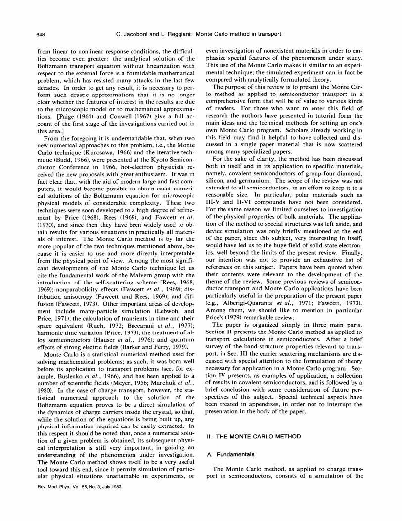
Figure 2 illustrates the principles of the method byshowing the simulation in k space and real space and theeffect of collecting statistics in the determination of thedrift velocity.
Definition of the physical system
The starting point of the program is the definition ofthe physical system of interest, including the parametersof the material and the values of physical quantities, suchas lattice temperature To and electric field. It is worthnoting that, among the parameters that characterize thematerial, the least known, usually taken as adjustable pa-rameters, are the coupling strengths describing the in-teractions of the electron with the lattice and/or extrinsicdefects inside the crystal.
At this level we also define the parameters that controlthe simulation, such as the duration of each subhistory,the desired precision of the results, and so on.
The next step in the program is a preliminary calcula-tion of each scattering rate as a function of electron ener-
gy. This step will provide information on the maximumvalue of these functions, which will be useful for optimiz-ing the efficiency of the simulation (see Sec. II.B.3). Fi-nally, all cumulative quantities must be put at zero in thispreliminary part of the program.
Ak=eE, (2. 1) 2. Initial conditions of motion
where k is the carrier wave vector, e its charge with itssign (e &0 for electrons and e&0 for holes), and fi thePlanck constant divided by 2m. . In this part of the simula-tion all quantities of interest, velocity, energy, etc. , arerecorded. Then a scattering mechanism is chosen as re-
sponsible for the end of the free flight, according to therelative probabilities of all possible scattering mechan-isms. From the differential cross section of this mechan-ism a new k state after scattering is randomly chosen asinitial state of the new free flight, and the entire process isiteratively repeated. The results of the calculation become
~In the present review, for brevity we shall often write "elec-trons" meaning in fact "charge carriers, " that is, electrons orholes indi fferently.
In the case under consideration, in which a steady-statesituation is simulated, the time of simulation must be longenough that the initial conditions of the electron motiondo not influence the final results. The choice of a "good"time of simulation is a compromise between the need forergodicity (t ~ oo ) and the request to save computer time.When a highly improbable initial value for the electronwave vector k is chosen, the first part of the simulationcan be strongly influenced by this inappropriate choice.
In the particular case of a very high electric field, if anenergy of the order of KYOTO {Kz being the Boltzmannconstant) is initially given to the electron, this energy wiH
be much lower than the average energy in steady-stateconditions, and during the transient it will increase to-wards its steady-state value. As a consequence, the elec-tron response to the field, in terms of mobility, may be in-
Rev. Mod. Phys. , Vol. 55, No. 3, July 1983

650 C. Jacoboni and L. Reggiani: Monte Carlo method in transport
DE F I NIT ION OF THE PHYSICAL SYSTEM
PUT OF PHYSICAL AND SiMULATION PARAMETERS
IN I T I AL COND IT IONS OF MOTION
STOCHASTIC DFTERMi NATION OF F L I GHT DURATION
1t
DETERMINATION OF ELECTRON STATE
J UST BEFORE SCAT TER ING
COLLECTION OF DATA FOR EST IMATORS
STOCHASTIC
DE T E R MINAT ION
OF SCATTERING
MECHA Nl S M
YESFi NAL
E VALUATION
OF E TiMATORS
STOCHAST I C
DE TE R Ml N A T I ON OF
ELECTRON STATE
JUST AFTER
SCAT TER I N 6
PRINT RESULTS
FIG. 1. Flowchart of a typical Monte Carlo program.
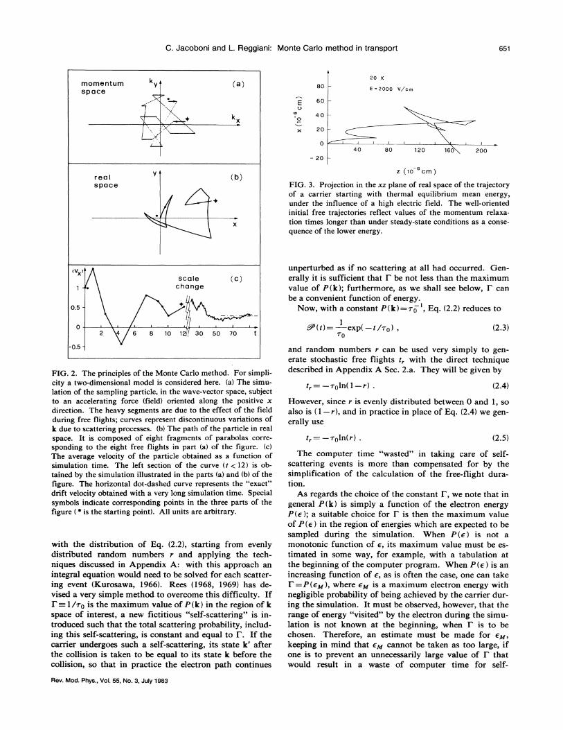
itially much higher than that of stationary conditions (seeSecs. II.C. 1 and IV.B.13). This is reflected in real spaceby initial free flights which are much longer than in sta-tionary conditions because of an abnormally largemomentum relaxation time initially (see Fig. 3).
The longer the simulation time, the less influence theinitial conditions will have on the average results; howev-er, in order to avoid the undesirable effects of an inap-propriate initial choice and to obtain a better convergence,the elimination of the first part of the simulation fromthe statistics may be advantageous. When the simulationis divided into many subhistories, better convergence tosteady state can be a=hieved by taking the initial state ofeach new subhistory as equal to the final state of the pre-vious one. In this way, only the initial condition of thefirst subhistory will influence the final results in a biasedway.
On the other hand, when a simulation is made to studya transient phenomenon and/or a transport process in anonhomogeneous system (for example, when the electrontransport in a small device is analyzed), then it is neces-sary to simulate many electrons separately; in this casethe distribution of the initial electron states for the partic-ular physical situation under investigation must be taken
into account (see Sec. II.C.1), and the initial transient be-comes an essential part of the results aimed at.
3. Flight duration —self-scattering
The electron wave vector k changes continuously dur-ing a free Aight because of the applied field according toEq. (2.1). Thus if P[ (kt)]dr is the probability that anelectron in the state k suffers a collision during the timedt, the probability that an electron which suffered a col-lision at time t=o has not yet suffered another collisionafter a time t is
exp —f P [k(t')]dt'
which, generally, gives the probability that the interval(O, t) does not contain a scattering. Consequently, theprobability H(t) that the electron will suffer its next col-lision during dt around t is given by
(t)d& =P[k(r)]exp —f P[k(t')]dt' dt . (2.2)
Because of the complexity of the integral at the ex-ponent, it is impractical to generate stochastic free flights
Rev. Mod. Phys. , Vol. 55, No. 3, July 1983
C. Jacoboni and L. Reggiani: Monte Carlo method in transport 651
momentumspace
(a} 80
60
20 K
E = 2OOO v/cm
40
20
—2040 80 120 16' 200
realspace
y n z (ip cm}
FIG. 3. Projection in the xz plane of real space of the trajectoryof a carrier starting with thermal equilibrium mean energy,under the influence of a high electric field. The well-orientedinitial free trajectories reflect values of the momentum relaxa-tion times longer than under steady-state conditions as a conse-quence of the lower energy.
&V &'
05-
unperturbed as if no scattering at all had occurred. Cxen-
erally it is sufficient that I be not less than the maximumvalue of P(k); furthermore, as we shall see below, I canbe a convenient function of energy.
Now, with a constant P(k) =rp, Eq. (2.2) reduces to
1H(t) = exp( t lrp), —70
(2.3)
-05-
FIG. 2. The principles of the Monte Carlo method. For simpli-
city a two-dimensional model is considered here. (a) The simu-
lation of the sampling particle, in the wave-vector space, subjectto an accelerating force (field) oriented along the positive xdirection. The heavy segments are due to the effect of the fieldduring free flights; curves represent discontinuous variations ofk due to scattering processes. (b) The path of the particle in real
space. It is composed of eight fragments of parabolas corre-sponding to the eight free flights in part (a) of the figure. (c)The average velocity of the particle obtained as a function ofsimulation time. The left section of the curve (t ~12) is ob-tained by the simulation illustrated in the parts (a) and (b) of thefigure. The horizontal dot-dashed curve represents the "exact"drift velocity obtained with a very long simulation time. Specialsymbols indicate corresponding points in the three parts of thefigure ( ~ is the starting point). All units are arbitrary.
with the distribution of Eq. (2.2), starting from evenlydistributed random numbers r and applying the tech-niques discussed in Appendix A: with this approach anintegral equation would need to be solved for each scatter-ing event (Kurosawa, 1966). Rees (1968, 1969) has de-vised a very simple method to overcome this difficulty. IfI:—I lrp is the maximum value of P(k) in the region of kspace of interest, a new fictitious "self-scattering" is in-troduced such that the total scattering probability, includ-ing this self-scattering, is constant and equal to I". If thecarrier undergoes such a self-scattering, its state k' afterthe collision is taken to be equal to its state k before thecollision, so that in practice the electron path continues
and random numbers r can be used very simply to gen-erate stochastic free flights t, with the direct techniquedescribed in Appendix A Sec. 2.a. They wi11 be given by
t, = —rpln(1 —r) . (2.4)
However, since r is evenly distributed between 0 and 1, soalso is (1 r), and —in practice in place of Eq. (2.4) we gen-erally use
t, = —rpln(r) . (2.5)
The computer time "wasted" in taking care of self-scattering events is more than compensated for by thesimplification of the calculation of the free-flight dura-tion.
As regards the choice of the constant I", we note that ingeneral P(k) is simply a function of the electron energyP(e ); a suitable choice for I is then the maximum valueof P(E) in the region of energies which are expected to besampled during the simulation. When P(E) is not amonotonic function of e, its maximum value must be es-timated in some way, for example, with a tabulation atthe beginning of the computer program. When P(e) is anincreasing function of e, as is often the case, one can takeI =P(eM), where eM is a maximum electron energy withnegligible probability of being achieved by the carrier dur-ing the simulation. It must be observed, however, that therange of energy "visited" by the electron during the sirnu-lation is not known at the beginning, when I" is to bechosen. Therefore, an estimate must be made for E'M,
keeping in mind that eM cannot be taken as too large, ifone is to prevent an unnecessarily large value of I thatwould result in a waste of computer time for self-
Rev. Mod. Phys. , Vol. 55, No. 3, July 1983

652 C. Jacoboni and L. Reggiani: Monte Carlo method in transport
I (e)= (2.6)
where e1
is a suitable threshold energy, and I"1
and I"2 arethe maximum values of P(e) in the two correspondingenergy ranges.
In using I"(e ) as given by Eq. (2.6), we should
(3
CC
I—
OCO
scattering events. One must also decide what action totake when, during the simulation, the electron energy ehappens to exceed the maximum value eM set up at thebeginning of the computer run. Some authors in such cir-cumstances arbitrarily reduce the electron energy e to avalue lower than e~ and simply check at the end of thecomputer run that such a situation occurred a limitednumber of times. This procedure may be dangerous, sinceit may obscure the occurrence of an indefinite increase ofelectron energy (electron runaway) when this happens atenergies above a critical value close to e,». A safermethod is to increase the value of eM and correspondinglyof I, if required, for the simulation to continue, withoutintervening in the electron energy. Since I" must be in-dependent of the simulated flight, it is always necessary tocheck that I has not been changed too many times. Thisis guaranteed when eM has been underestimated at the set-
up of the program run, because it will quickly increase toa value above which the electron energy will rarely go.
For a semiconductor model that contains several val-
leys, a different value of EM may be appropriately takenin each type of valley.
Sometimes the total scattering probability P(e) has alarge variation around some threshold value due to astrong scattering mechanism with a given activation ener-
gy (a typical case is intervalley scattering from central toupper valleys in polar semiconductors). In this case, asingle value of I may result in a very large number ofself-scattering events at low electron energies (see Fig. 4).It is then possible to introduce a step-shaped scatteringrate I (e) given by
remember that, during a free flight, the electron energymay exceed the va1ue el. The following two cases mayoccur according to the initial state of the free flight ~
(i) An electron begins a free flight with an energy belowel ~ A random number r is then used to generate with I
1
a free flight with duration t, given by
I.,= —~1ln(r) . (2.7)
If at the end of this free flight the electron energy is stillfess than e1, t„ is retained, and the simulation proceeds asusual. If, on the contrary, at the end of this free flight theelectron energy is above el, t, as given by Eq. (2.7) cannotbe retained. The same random number r is then used togenerate a new duration of the free flight as follows.From Eq. (2.6) we have, instead of Eq. (2.3),
lexp( —tlri), t &t
7](~)=
1expI —[tlri+(t —l)lr2]l, t) t
72
(2.&)
where t is the time necessary for the electron to reach theenergy e1 and can be easily evaluated from the electrondynamics. By application of the direct technique (see Ap-pendix A Sec. 2.a) t, is then given by
t, = —r2ln(r)+t(1 —r2iri) . (2.9)
4. Choice of the scattering mechanism
(ii) An electron begins a free flight with an energyabove el. The duration of this free flight can always bedetermined by Eq. (2.6) with r=r2. In fact, even if thefinal enery is below e1, one is justified in considering theupper value I 2 of I (c ) extended to lower energies, as longas this is done independently of the particular value of r.Of course, I"2 must then be consistently considered in thedetermination of the scattering mechanism (in particularfor self-scattering) which caused the end of the free flight(see next section).
The only situation not accounted for in the above dis-cussion is when, during a single free flight, the electronenergy starting from values below e1 first increases toabove e1 and then decreases to below e1', but this situationcannot occur with static fields and normal band struc-tures.
The above idea can be extended to piecewise functionsI (e) with more than one step. However, such a pro-cedure must be compared, from the point of view of sav-ing computer time, with the so called fast self-scatteringtechnique (see next section).
ENERGY (arb. units)
FIG. 4. Sketch of a two-level step-shaped total scattering rate,including self-scattering I (e ), appropriate for reducing thenumber of self-scattering events with respect to a single-levelchoice (the I 2). 1 1 is used for energies between 0 and e~, as ex-plained in the text. The shaded region illustrates the increasedefficiency resulting from the two-level choice.
During free flight, electron dynamics is governed byEq. (2.1) so that at its end the electron wave vector andenergy are known, and all scattering probabilities P;(e)can be evaluated, where i indicates the ith scatteringmechanism. The probability of self-scattering will be thecomplement to K' of the sum of the P s. A mechanismmust then be chosen among all those possible: given a
Rev. Mod. Phys. , Vol. 55, No. 3, July 1983

C. Jacoboni and L. Reggiani: Monte Carlo method in transport 653
random number r, the product rI is compared with thesuccessive sums of the P s, and a mechanism is selectedas described in Appendix A Sec. 2.d.
Since each scattering probability P;(e) must be evaluat-ed unti1 a mechanism is chosen by the random number, inthe computer program it is convenient to rank the P s inorder of probability before beginning. It must be noted,however, that the occurrence of the various scatterings de-pends also on temperature and field strength, so that itmay sometimes be difficult to predict their relative fre-quency.
If all scatterings have been tried and none of them hasbeen selected, it means that r I & P(e ), and a self-scattering occurs. Ascertaining by this procedure that aself-scattering occurs is therefore most time consuming,since all P s must be explicitly calculated. However, theprocess may be shortened by use of an expedient thatmight be called fast self-scattering. It consists of settingup a mesh of the energy range under consideration at thebeginning of the simulation and then recording in a vectorthe maximum total scattering probability P' ' in each en-
ergy interval b,e' ' (energy intervals equally distributed ona logarithmic scale may be useful). At the end of theflight if the electron energy faIls in the nth interval, be-fore trying all P s separately, one compares rt with P'"'.At this stage if rI &P "' then a self-scattering certainlyoccurs; otherwise all P s will be successively evaluated.Thus only when P(e) ~ rI &P'"' does a self-scattering oc-cur which requires the evaluation of all P s.
As regards the scat tering probabilities of variousmechanisms and their use in the Monte Carlo program,we shall consider in Sec. III the cases useful for covalentsemiconductors. For other cases we refer the reader tothe original literature.
5. Choice of the state after scattering
Once the scattering mechanism that caused the end ofthe electron free flight has been determined, the new stateafter scattering of the electron, k, must be chosen as thefinal state of the scattering event. If the free flight endedwith a self-scattering, k, must be taken as equal to k~, thestate before scattering. When, in contrast, a true scatter-ing occurred, then k, must be generated, stochastically,according to the differential cross section of that particu-lar mechanism. The techniques used to select the stateafter each particular type of scattering are discussed inSec. III.D.
gy, etc.) during a single history of duration T asT(~)T =—I W[k(t)]dr
E.
M[k(t' }]dr',T (2.10)
b. Synchronous ensemble
Another method of obtaining an average quantity (W)from the simulation of a steady-state phenomenon hasbeen introduced by Price (1968, 1970); this is thesynchronous-ensemble method. Let us consider Fig. 5, inwhich a time axis is specified for each of the N electronsof the physical system. Circles in these axes indicatescat tering events. In principle, each of the axes canrepresent a simulated electron, and self-scattering can beincluded if wanted. In general the averge value of a quan-
90—O--CM
3
where the integral over the whole simulation time T hasbeen separated into the sum of integrals over all freeflights of duration t;. When a steady state is investigated,T should be taken as sufficiently long that (M)T in Eq.(2.10) represents an unbiased estimator of the average ofthe quantity .V over the electron gas.
In a similar way we may obtain the electron distribu-tion function: a mesh of k space (or of energy) is set up atthe beginning of the computer run; during the simulationthe time spent by the sample electron in each cell of themesh is recorded and, for large T, this time convenientlynormalized will represent the electron distribution func-tion, that is, the solution of the Boltzmann equation(Fawcett er al. , 1970). This evaluation of the distributionfunction can be considered a special case of Eq. (2.10} inwhich we choose for M the functions nj(k) with value 1
if k lies inside the jth cell of the mesh and zero otherwise.This method is the one most generally used to obtain
transport quantities from Monte Carlo simulations. Weshall see specific applications of it in Sec. IV.
6. Collection of results for steady-state phenomena
The data collected at each free flight will form the basefor the determination of the quantity of interest.
oc
TlME (arb. units )
a. Time averages
Generally speaking, we may obtain the average value ofa quantity .M[k(t)] (e.g. , the drift velocity, the mean ener-
FIG. S. Sketch illustrating the synchronous-ensemble method.Subscripts (1,2,3. . . , N) label the time axis of the ith particle;open circles indicate scattering events; t is the generic time of asteady-state condition.
Rev. Mod. Phys. , Vol. 55, No. 3, July 1983

654 C. Jacoboni and L. Reggiani: Monte Carlo method in transport
tity M is defined as the ensemble average at time t overthe N electrons of the system, n(k)= 1
nb(k)r(k)70
(2.13)
(M) = —g M;(t; =t) .1
N(2.11)
In particular, the steady-state distribution function is pro-portional to the number of electrons n (k}b,k that at time tare found to be in a cell of fixed volume Ak around k.Then Eq. (2.11) can also be evaluated as
where ~0 is an appropriate normalization constant. If, byincluding self-scattering, we use a constant r(k), then thesteady-state distribution function becomes proportional tothe before-scattering distribution
n(k) ~nb(k)
(.ur ) = K g n (k)M(k), (2.12)and Eq. (2.12) can be used in a Monte Carlo simulation inthe following form:
where ' is an appropriate normalization constant, andn (k) can be considered as proportional to the probabilityof finding any given electron in state k.
Now, in the spirit of Chambers's path-integral method(Chambers, 1952), an electron will be found in k at time tif it has been scattered in the suitable k' an appropriatetime interval t' before t and has not been scattered againbetween (t —t') and t (see Fig. 6).
Let n, (k) be the so-called after-scattering distributionfunction, proportional to the probability that an electronis found in k immediately after a scattering event. Thenn (k) is proportional to
(2.14)
where the sum covers all N electron free flights, and Ms;indicates the value of the quantity W evaluated at the endof the free flight immediately before the ith scatteringevent.
If self-scattering with a step-shaped total scatteringprobability, as described in Sec. II.B.3, is used, then thevarious terms in the sum of Eq. (2.14) must be weightedwith a factor I '(k); but in this case particular care mustbe taken when, during a flight, k(t) crosses the borderfrom one value of I; to another value, since r(k) must bea unique, well-defined function of k.
where H(k', t') is the probability that an electron in k' ata given time will not be scattered before an interval oftime t'.
If we now consider the before-scattering distributionfunction nb(k}, proportional to the probability that anelectron is found in k immediately before a scatteringevent, we shall find by an argument similar to that givenabove that
nb(k) cc f n, [k'(t')]H[k'(t'), t']dt'r(k)
where r '(k) is the scattering rate for an electron in k.Thus the steady-state distribution function is given by
c. Statistical uncertainty
In order to estimate the statistical uncertainty of atime-average result (M) r due to the finite value of thesimulation time T, as mentioned in Sec. II.B, we candivide' the whole history in N subhistories of durationT/N; for each of them a value (M)t is obtained. Wemay then take as the most probable value of (M) theaverage of the (.Gt')t's (which will be equal to (M) r)and its standard deviation as the statistical uncertainty on(.ot')r. The subhistories must be sufficiently long to beconsidered as independent of each other, but sufficientlyshort to allow us to perform a large number N of them.
FIG. 6. Trajectory of an electron in k space. An electron thatcontributes to the distribution function f(k, t) must have scat-tered onto the trajectory at some previous time t' at the corre-sponding k' and have followed it without scattering until it ar-rived at point k at time t (Cohen et al. , 1960).
It may seem strange that with a constant r(k) the before-scattering distribution nq(k) is equal to the steady-state distribu-tion, since the states just before the scattering events seem to beinfluenced "at the maximum" by the applied fields. However,one should consider that, while nq(k) weights equally all freeflights (short and long ones) with average duration v., when aninstantaneous picture of the electron gas is taken at any time t,longer free flights are more likely to be caught. In other words,in the latter case the vertical line in Fig. 5 crosses free flightswhose mean duration is longer than the average over all freeflights; in fact, the distribution of the hemi-flights on the rightand on the left of the line t reproduces the distribution of flightdurations, so that the average length of the flights crossed by t
is 27.This division requires the interruption of a free flight at the
end of each subhistory simulation. The remaining part of theflight is thus used as the initial part of the successive subhistorysim ulation.
Rev. Mod. Phys. , Vol. 55, No. 3, July 1983

C. Jacoboni and L. Reggiani: Monte Carlo method in transport 655
In this case the uncertainty decreases as I/~N. Further-more, it is possible to carry out, on the series of partial re-sults (.cl)1, those tests (Hammersley and Handscomb,1964) which verify the statistical nature of their fluctua-tions.
C. Time- and space-dependent phenomena
For time- and/or space-dependent problems the analyt-ical solution of the Boltzmann equation is even more dif-ficult than for homogeneous and stationary problems,while for Monte Carlo programs little work need be addedto attack such problems. This confirms again the useful-ness of the Monte Carlo method, in particular, for theanalysis of small devices, where it is often necessary toconsider both the transient dynamic response to the volt-age changes and electronic behavior at different points ofthe device with different field or material properties (Bac-carani et al. , 1977; Zimmermann and Constant, 1980).
As mentioned ir~ Sec. II.A, for such problems we can-not rely on the ergodicity of the system; an ensemble ofparticles must be explicitly simulated (Lebwohl and Price,1971a, 1971b).
One exception of this rule that will be discussed in Sec.II.C.3 is that of phenomena which are periodic in spaceand/or time. In this case the different situations experi-enced by the electron in equivalent positions or times willtake into account the many possibilities of various parti-cles, and again the simulation of a single electron mayyield the necessary information about the entire electrongas.
1. Transients
We shall consider here the case of a homogeneous elec-tron gas with time-dependent behavior. In particular, it isof interest to study the transient dynamic response to asudden change in the value of an applied field. In this sit-uation many particles must be independently simulatedwith appropriate distributions of initial conditions. Pro-vided the number of simulated particles is sufficientlylarge, the average value of a quantity of interest, obtainedon this sample ensemble as a function of time, will berepresentative of the average for the entire gas.
It must be stressed that the estimators given by Eqs.(2.10) and (2.14) are based on the hypothesis of steady-state conditions and cannot be used when a time-dependent phenomena is analyzed: the ensemble averageof a quantity M must actually be estimated according toits definition, given by Eq. (2.11):
(2.15)
where i runs over all N simulated particles.The duration of the transient response is not known a
priori and will be of the order of the largest of the charac-teristic times of the electron system. This time may becalled the "transient-transport time" and in general de-
pends upon the values of the applied field and tempera-ture; in our case of high-field transport in semiconduct-ors, it may roughly correspond to the energy relaxationtime or to the time for repopulation of different valleys.
To determine the precision of the results obtained, oneseparates the entire ensemble into a certain number ofsubensembles and estimates for each of them the quantityof interest .V. Then their average value and standard de-viation can be taken, respectively, as the most probablevalue and the statistical uncertainty of .N.
The transient dynamic response obtained by means ofthe simulation will, of course, depend upon the initialconditions of the carriers, and these must be assumed ac-cording to the situation to be explored. Initial velocitydistributions which may be of interest are, for example, aMaxwellian distribution at the lattice temperature and nodrift, or a Maxwellian distribution with an electron tem-perature higher than that of the lattice, with or withoutdrift.
2. Space-dependent phenomena
The simulation of a steady-. -.tate phenomenon in aphysical system where electron transport depends uponthe position in space is of particular interest for theanalysis and modeling of devices. For this case, too, anensemble of independent particles must be used, and aver-ages must be taken over particles at given positions. Thestatistical uncertainties of the results can be obtained withsubensembles, as indicated in the preceding section.
In a steady-state situation, particles enter the region ofinterest continuously, and in the simulation some initialwave vector must be assumed when a new particle is con-sidered, according to the momentum distribution of theparticles in the physical system under investigation. Forexample, a cold hemi-Maxwellian distribution, that is, onewith only positive velocity components along a givendirection, may be convenient in simulating the metalliccontact of a device. If the simulated electron entering thedevice goes back to the contact, a new electron must begenerated, but the "lost" electron must be accounted forin the final results in a way that depends on the particularanalysis being carried out.
Space- and time-dependent phenomena may presentsimilar characteristics, and they have sometimes beenconfused in simulation problems. For instance, if a fieldis suddenly switched on from zero to a large value, duringthe initial transient the drift velocity reaches values largerthan those in steady-state conditions (overshoot effect),and this effect is sornetirnes useful in discussing thebehavior of an electron stream, coming from a low-fieldregion and entering a region with a high applied field.
If this mode of reasoning is correct from a qualitativepoint of view, in rigorous calculations the kind of averagethat must be taken is different depending on whethertime- or space-dependent phenomena are considered. In asteady-state phenomenon with space-dependent appliedfields it is, in general, necessary to consider the electronproperties at given positions (Baccarani et al. , 1977; Zim-
Rev. Mod. Phys. , Vol. 55, No. 3, July 1983
C. Jacoboni and L. Reggiani: Monte Carlo method in transport
mermann and Constant, 1980), so that the simulationmust record average values for given points over time;when the object of the investigation is the evolution intime of a homogeneous sytem, average quantities must beevaluated at given times independent of the particle posi-tions.
Eo+E
3. Periodic fields
Monte Carlo simulation can be extended to permit cal-culation of the response of charge carriers to periodicexternal fields of any strength (Lebwohl, 1973; Zimmer-man et al. , 1978). If a field
E=Ep+ E) sin(cot ) (2.16)
is applied, and the ac term is small enough to be in thelinear-response regime, the average electron velocity willbe of the form
Eo —E)
c
L4Q
I—O0UJ
4I
4I 4I
T= Nht
4I
4I4I 04P 4I II
e ~4I
SI te e ~ e e4I ~ ~
( v(t ) ) =vp+ vi sin(fur ) + vq cos((a)1 ) (2.17)I—LL
OC
Ot(+2T
1 2'At= ——% cg
(2. 18)
Then we average the values of v obtained at timeslhr, (l+X)ht, (i+2K)ht, . . . . The result is an estimatorof the average electron velocity (v), which is a periodicfunction of t with the same period 2n. /co, at the timesgiven above.
The synchronous-ensemble method described in Sec.II.B.6.b for static fields has been extended by Lebwohl(1973) to include the case of periodic fields. The result isa simple parametric dependence of Eq. (2.13) upon time:
n(k, t) = nb(k, t)r(k)1
7 0(2.19)
and in the applications it is possible to operate as for stat-ic fields with the additional care of assigning each
The coefficients vl and v2 of the fundamental responsein Eq. (2.17) can be obtained as sine and cosine Fouriertransforms, respectively, of the velocity of the simulatedelectron over its history. Since the equation of motion ofthe particle subject to a field given by Eq. (2.16) is knownin explicit terms, the Fourier coefficients vl and v2 caneasily be obtained by the simulation (Lebwohl, 1973).
For large periodic fields, the periodic part of thecurrent will contain higher harmonics, besides the funda-mental frequency. These components can also be ob-tained by Fourier analysis of the simulated velocity, butin this case statistical-noise problems become severe.
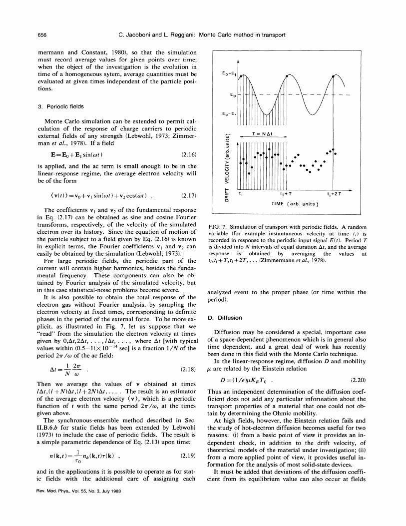
It is also possible to obtain the total response of theelectron gas without Fourier analysis, by sampling theelectron velocity at fixed times, corresponding to definitephases in the period of the external force. To be more ex-plicit, as illustrated in Fig. 7, let us suppose that we"read" from the simulation the electron velocity at timesgiven by O, b, t, 2ht, . . . , Ibt, . . . , where ht [with typicalvalues within (0.5—1)X10 ' sec] is a fraction 1/%of theperiod 2m /m of the ac field:
(srb. units)
FIG. 7. Simulation of transport with periodic fields. A randomvariable (for example instantaneous velocity at time t; ) isrecorded in response to the periodic input signal E(t). Period Tis divided into N intervals of equal duration At, and the averageresponse is obtained by averaging the values att;, t;+ T, t;+2T, . . . (Zimmermann et al. , 1978).
analyzed event to the proper phase (or time within theperiod).
D. Diffosion
Diffusion may be considered a special, important caseof a space-dependent phenomenon which is in general alsotime dependent, and a great deal of work has recentlybeen done in this field with the Monte Carlo technique.
In the linear-response regime, diffusion D and mobilityp are related by the Einstein re1ation
D =(1/e)pK~Tp (2.20)
Thus an independent determination of the diffusion coef-ficient does not add any particular information about thetransport properties of a material that one could not ob-tain by determining the Qhmic mobility.
At high fields, however, the Einstein relation fails andthe study of hot-electron diffusion becomes useful for tworeasons: (i) from a basic point of view it provides an in-
dependent check, in addition to the drift velocity, oftheoretical models of the material under investigation; (ii)from a more applied point of view, it provides useful in-formation for the analysis of most solid-state devices.
It must be added that deviations of the diffusion coeffi-cient from its equilibrium value can also occur at fields
Rev. Mod. Phys. , Vol. 55, No. 3, July 3983
C. Jacoboni and L. Reggiani: Monte Carlo method in transport
lower than those at which hot-electron phenomena areusually present, because of the possibility of intervalleydiffusion, which occurs in many-valley semiconductors(see Sec.IV.B.3).
the mth moment of n (z), defined by
M =—fz n(z)dz1 (2.25)
Fick diffusion
Diffusion is described at a phenomenological level bythe first Fick's equation,
(X being the total number of particles), then from Eq.(2.24) we have, after successive integrations by parts(Jacoboni et al. , 1978; Price, 1979),
dMl
dt=V
(2.21)dM2
dt2vdll +2D
(2.26)where j is the current density, D;J is the diffusion tensor,x is the particle position in space, and n(x) is the particledensity; the sum over repeated indices is implied.
If an electric field is also present which would produce,in the absence of diffusion, a drift velocity ud, and if dif-fusion and drift do not influence each other, then for Eq.(2.21) we substitute
j, =e n(x}v„(E)—DJBn(x)
Bxj(2.22)
By combining this equation with the continuity equation,
Bne = — j;Bt Bx;
(2.23)
we obtain the diffusion equation, sometimes called thesecond Fick's equation:
Bn Bn 92n- =- —vd (E) +DJat ax, " ax, ax,-(2.24)
4This is not a trivial point ~ For example, let us consider anopen-circuit situation with a high applied electric field. Herediffusion and drift cancel each other out to produce a vanishingnet current. They influence each other in that the electron ener-
gy distribution function is not the usual hot-electron distributionobtained for a homogeneous system, because power does notflow through the particle gas, and yet electrons experience ahigh field between successive collisions. A similar situation is
realized within the space-charge region of a p-n junction in
open-circuit conditions.
where vd and D have been supposed to be space indepen-dent.
Under linear-response conditions, vd depends linearlyon field, and D is field independent, as can be obtainedfrom the solution of the Boltzmann equation. The gen-eralization at high fields of Eq. (2.24) is usually per-formed by assuming D =D(E). As a matter of fact, arigorous derivation from the Boltzmann equation of Eq.(2.24) with D =D(E) can be performed only by assumingsmall concentration gradients and times longer than boththe transient-transport time, defined in Sec. II.C. I, andthe time necessary for setting up the correct space-velocity correlations (see Gantsevich et al. , 1974, 1979).
If, for simplicity, n is assumed to be a function of onlyone coordinate z parallel to the direction of vd, and M is
dM
dt=mvdM ~+m (I —1)DIM~
where DI is the diagonal component of D along vd.In particular, for the second central moment we have
D[= ——&(z —&z)) )1 d2 dt
(2.27}
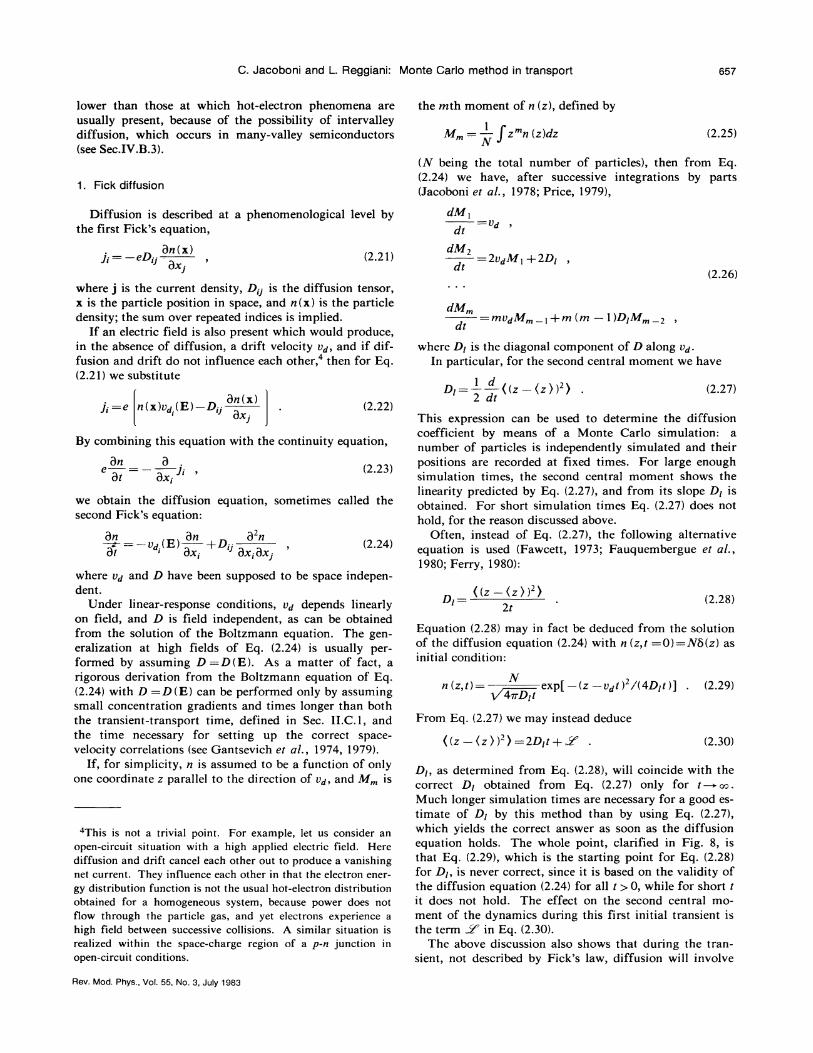
This expression can be used to determine the diffusioncoefficient by means of a Monte Carlo simulation: anumber of particles is independently simulated and theirpositions are recorded at fixed times. For large enoughsimulation times, the second central moment shows thelinearity predicted by Eq. (2.27), and from its slope D& isobtained. For short simulation times Eq. (2.27) does nothold, for the reason discussed above.
Often, instead of Eq. (2.27), the following alternativeequation is used (Fawcett, 1973; Fauquembergue et al. ,
1980; Ferry, 1980):
&(z —&z) )')I 2t
(2.28)
Equation (2.28) may in fact be deduced from the solutionof the diffusion equation (2.24) with n (z, t =0)=%5(z) asinitial condition:
n(z, t)= exp[ —(z vdt) i (4D—It)] . (2.29)X 2'
/4~D&t
From Eq. (2.27) we may instead deduce
&(z —&z))-') =2D, t+ W . (2.30)
DI, as determined from Eq. ( .28), will coincide with thecorrect DI obtained from Eq. (2.27) only for t~ &n.
Much longer simulation times are necessary for a good es-timate of D~ by this method than by using Eq. (2.27),which yields the correct answer as soon as the diffusionequation holds. The whole point, clarified in Fig. 8, isthat Eq. (2.29), which is the starting point for Eq. (2.28)for DI, is never correct, since it is based on the validity ofthe diffusion equation (2.24) for all t & 0, while for short tit does not hold. The effect on the second central mo-ment of the dynamics during this first initial transient isthe term W in Eq. (2.30).
The above discussion also shows that during the tran-sient, not described by Fick s law, diffusion will involve
Rev. Mod. Phys. , Vol. 55, No. 3, July 1983
658 C. Jacoboni and L. Reggiani: Monte Carlo method in transport
is divided into a number N of intervals, of durationb, T =T/N, in order to determine C(t) at times O, b, T,25T, . . . , NET = T. During the simulation, the velocityof the sample particle is recorded at the time values ihT,i =0, 1,2, . . . . When i becomes greater than or equal toN, the products,
u(ib, T)v [(i j)—b.T], j=0, 1,2, . . . , N
are evaluated for each i. Products corresponding to thesame value of i are averaged over the simulation, thus ob-taining
u(t)u(t +j b, T) =C(j b, T)+u~ (2.34}
since in a steady-state situation the ensemble average isincluded in the time average.
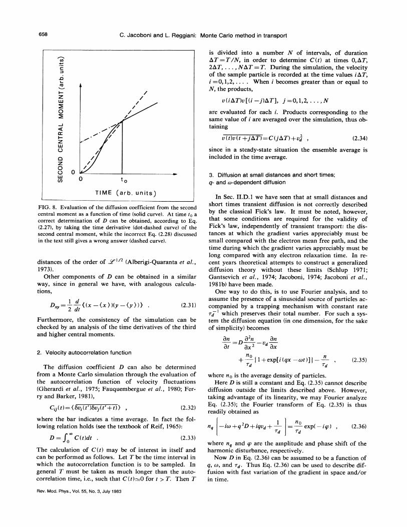
0 t p3. Diffusion at small distances and short times;q- and ~-dependent diffusion
TIME (arb. units)
FIG. 8. Evaluation of the diffusion coefficient from the secondcentral moment as a function of time (solid curve). At time to acorrect determination of D can be obtained, according to Eq.(2.27), by taking the time derivative (dot-dashed curve) of thesecond central moment, while the incorrect Eq. (2.28) discussedin the text still gives a wrong answer (dashed curve) ~
distances of the order of M' (Alberigi-Quaranta et al. ,1973).
Other components of D can be obtained in a similarway, since in general we have, with analogous calcula-tions,
(2.3 1)
Furthermore, the consistency of the simulation can becheeked Oy an analysis of the time derivatives of the thirdand higher central moments.
2. Velocity autocorrelation function
C; (t)= &5u;(t')5vj(t'+t) & (2.32)
The diffusion coefficient D can also be determinedfrom a Monte Carlo simulation through the evaluation ofthe autocorrelation function of velocity fluctuation(Gherardi et al. , 1975; Fauquembergue et al. , 1980; Fer-ry and Barker, 1981),
no+ I 1+exp[i (qx tot )] )——
7d(2.35)
where no is the average density of particles.Here D is still a constant and Eq. (2.35) cannot describe
diffusion outside the limits described above. However,taking advantage of its linearity, we may Fourier analyzeEq. (2.35); the Fourier transform of Eq. (2.35) is thusreadily obtained as
In Sec. II.D. 1 we have seen that at small distances andshort times transient diffusion is not correctly describedby the classical Fick's law. It must be noted, however,that some conditions are required for the validity ofFick's law, independently of transient transport: the dis-tances at which the gradient varies appreciably must besmall compared with the electron mean free path, and thetime during which the gradient varies appreciably must belong compared with any electron relaxation time. In re-cent years theoretical attempts to construct a generalizeddiffusion theory without these limits (Schlup 1971;Gantsevich et al. , 1974; Jacoboni, 1974; Jacoboni et aI. ,1981b) have been made.
One way to do this, is to use Fourier analysis, and toassume the presence of a sinusoidal source of particles ac-companied by a trapping mechanism with constant rate7d
' which preserves their total number. For such a sys-tem the diffusion equation (in one dimension, for the sakeof simplicity) becomes
Bn 9 n Bn
Bt Qx2 9x—Ud
where the bar indicates a time average. In fact the fol-lowing relation holds (see the textbook of Reif, 1965):
1nq —ico+q D+iqUd+
7d
noexp( —i y)
7d(2.36)
D= C(t}dt (2.33)
The calculation of C(t) may be of interest in itself andcan be performed as follows. Let T be the time interval inwhich the autocorrelation function is to be sampled. Ingeneral T must be taken as much longer than the auto-correlation time, i.e., such that C(t)=0 for t ~ T. Then T
where nq and y are the a][nplitude and phase shift of theharmonic disturbance, respectively.
Now D in Eq. (2.36}can be assumed to be a function ofq, co, and 7d. Thus Eq. (2.36) can be used to describe dif-fusion with fast variation of the gradient in space and/or1n time.
Rev. Mod. Phys. , Vol. 55, No. 3, July 1983

C. Jacoboni and L. Reggiani: Monte Carlo method in transport
By using Chamber's methods, we can write a formalsolution of Eq. (2.36) (Jacoboni et al. , 1981b), that yieldsan expression for D(q, co, rd) which can be used in MonteCarlo calculations:
1D(q, cv, rd }= [1 —R +irdR(cv —qvd)]
q v.dR
(2.37)
T 2
S„(co)= lim — f 5v(t)exp(icot}dtT ~ T
(2.40)
Now the Wiener-Khintchine theorem connects the auto-correlation function C(t) and S„(cv ) through
S„(cv)=2f C(t)exp(icvt)dt
By taking into account Eq. (2.39), we obtain
with S„(cv ) =2D (cv ) (2.41b)
oo dg aoR= dx 'exp i ( qx—'cv t ')——
0 gd —oo id
(2.38)
D(co)= f C(t) exp(icvt)dt (2.39)
In order to obtain D(q, cv, r~) from a Monte Carlosimulation, it is sufficient to include among the scatter-ings a trapping mechanism with a constant inverse rate
If the particle is trapped after it has covered a dis-tance x' in a time t' the quantity exp[ i (qx' —cot')] is-recorded. Then R (q, co, rd ) is obtained as the mean valueof this quantity, since the simulation automatically ac-counts for the weighting factor.
After a trapping process the particle starts again with avelocity chosen according to the desired initial conditions.If the particle starts with the velocity it had when de-cayed, the initial conditions are taken according to thesteady-state distribution of velocities. In any case, for ~dsufficiently long, the results will be independent of the in-itial conditions assuined. For short rd, results for the dif-fusivity are obtained for the transient transport regime ac-cording to the initial conditions assumed. Finally, we ob-serve that Eq. (2.39) can be used to determine D(cv ) in aMonte Carlo procedure, by determining the autocorrela-tion function C(t},as described in the preceding section.
4. Noise and diffusion
Recently much interest has been shown (Hill et al. ,1979; Fauquembergue et al. , 1980} in the use of MonteCarlo techniques to determine the noise spectrum of velo-city fluctuations in connection with diffusion.
If we consider, again for simplicity, a one-dimensionalsituation, the power spectrum of the velocity fluctuationsis defined as
where H( x', t') is the probability density that, in the ab-sence of trapping, a particle covers a distance x' in a timet'. D(q, co } can be obtained as a special case of the aboveresult in the limit td~ ao.
For co =0, an expression of D(q) is easily obtained foruse on steady-state phenomena with strong spatial varia-tion.
For vanishing q it is possible to obtain an extension ofEq. (2.33}valid for an arbitrary frequency,
This result shows that a determination of the noisespectrum of the velocity fluctuations is equivalent to thedetermination of the frequency-dependent diffusivity.Thus the noise spectrum can be obtained as the Fouriertransform of C(t), as indicated for D( cv) in Sec. II.D.3.On the other hand, Eq. (2.40) can be used directly, notonly for the determination of S„(cv}, but also for thedetermination of D(cv) in a Monte Carlo simulation. Anaverage, over a particle ensemble, of the absolute squaredFourier transform of the electron velocity must be taken.
E. Ohmic mobility
When the Monte Carlo method is used to obtain thedrift velocity of charge carriers at low applied fields, thestatistical uncertainty originating from thermal motionmay become particularly large. Qf course, in principle,apart from the round-off errors of the computer, anydesired precision can be obtained, but the computer timenecessary for a high degree of precision often makes sucha run impractical and expensive.
The uncertainty due to thermal motion is particularlybothersome when the Ohmic mobility is sought. For thiscase, however, it is possible to evaluate the diffusion coef-ficient at zero field with one of the methods discussed inSec. II.D and then to obtain the Ohmic mobility by meansof the Einstein relation [see Eq. (2.20}]. It is worth notingthat when no external field is applied, the energy —andtherefore the scattering probability of the particle —isconstant during a free flight, so that no self-scatteringneed be introduced.
At low fields, another difficulty may arise when wedeal with many-valley semiconductors. Intervalleyscattering is due to phonons with a minimum equivalenttemperature of the order of at least 100 K. If the latticetemperature is well below such a value, intervalley pho-non absorption is almost absent because very few phononsare present in the crystal with that energy and, at lowfields, the electron energy very rarely reaches values suchas to make intervalley phonon emission possible. As aconsequence, the Monte Carlo simulation may proceedfor very long times without any valley change of the sam-pling electron. In this situation it is very difficult to ob-tain a correct estimate of the valley populations.
When Ohmic conditions are analyzed and no interval-ley transition is present at all, this difficulty may be over-corne by simulating one electron in each valley, since weknow a priori that the populations of all valleys must bethe same. Gn the other hand, when we enter the field re-
Rev. Mod. Phys. , Vol. 55, No. 3, July 1983

660 C. Jacoboni and L. Reggiani: Monte Carlo method in transport
gion in which a repopulation occurs and intervalley tran-sitions are very rare, the Monte Carlo method becomesinefficient. We shall return to this point in Sec. II.Hwhen we consider several variance-reducing techniques.
F. Impact ionization
The impact ionization rate col can be obtained from theMonte Carlo method by introducing the probability ofimpact ionization as an independent scattering mechan-ism which is added to phonon and impurity scatterings(Lebwohl and Price, 1971a; Curby and Ferry, 1973; Shi-chijo et al. , 1981;Skichijo and Hess, 1981).
When an ensemble Monte Carlo method is used, theimpact ionization process can be examined as follows(Lebwohl and Price, 1971a). The energy of the minoritycarrier (of the electron-hole pair created) relative to theband edge is neglected and the carrier itself is disregarded.Therefore the sum of the two majority-carrier final ener-gies (ef &+ef2) equals (e —eg) where e is the initial energyand eg the energy gap. After each ionization process, oneof the resulting (%+ I) particles, chosen at random, iseliminated to maintain a fixed sample size. The pair gen-eration rate per particle per unit time, gl, is obtained bycounting ionization events; it is converted to impact ioni-zation rate by
(2.42)
In other papers (Curby and Ferry, 1973; Shichijo et al. ,1981; Shichijo and Hess, 1981) a single-particle MonteCarlo simulation is used, and when impact ionization oc-curs the created electron-hole pair is disregarded. Theimpact ionization rate has been obtained by averaging thedistance to impact ionization over a sufficient number ofionizations, as in Eq. (2.42)
perpendicular to B, as shown in Fig. 9. A Monte Carlosimulation performed with such a geometry of fields foran infinite homogeneous sytem yields the drift velocityvd, and in particular the two components v~ and U, paral-lel and perpendicular to E, and the angle 0 formed by vdand E.
At this point we may interpret the results of the simu-lation in two different physical ways (Boardman et al. ,1971), according to the particular system under considera-tion.
One interpretation corresponds to the case of a longsample. The electric field E is decomposed into two com-ponents E„parallel to vd, which must be considered asthe applied field, and EH, perpendicular to both 8 and vd,which must be considered as the Hall field [see parts (a)and (b) of Fig. 9]. In this case the drift mobility pd isdetermined by
Vd UdPd= E, E cosO
(2.45)
while the Hall mobility is
EHPH= BE (2.46)
Therefore, from the Monte Carlo simulation it is possibleto obtain a direct determination of the Hall scattering fac-tor rH given by
PHPH=
Pd BUd(2.47)
This number is of particular interest, since it dependsupon the particular type of scattering mechanism thatcontrols the transport process.
The second interpretation corresponds to the case of
G. Magnetic fields
The scope of the Monte Carlo method can be extendedto include the case where both magnetic and electric fieldsare present. In this case the equation of motion of a car-rier during a free flight will be
Ea
vRc=e E+—)& 8C
(2.43)i) Vd
where 8 is the magnetic field, c the light velocity in vacu-um, and v the group velocity of the particle,
(2.44)B
Apart from this change in electron dynamics, the wholeMonte Carlo simulation proceeds as usual (Boardmanet a/. , 1971; Chattopadhyay, 1974), but the drift velocitywiH not, in general, be parallel to the applied electric field.Loss of cylindrical symmetry requires in this case a fullthree-dimensional simulation, even with very simplemodels. With a spherical band and a magnetic field 8orthogonal to E, the drift velocity vd is also in the plane FIG. 9. Geometry for 8, E, and vq {see text).
Rev. Mod. Phys. , Vol. 55, No. 3, July 1983

C. Jacoboni and L. Reggiani: Monte Carlo method in transport 661
very short flat samples in which the electrons can movefrom one contact to the other at the Hall angle 0 withrespect to the applied field, thus producing a transversecurrent and no Hall field [see part (c) of Fig. 9]. Thelongitudinal mobility in this case is obtained as
UI vdpp = = cosO =pd cos 0
F. E (2.48)
For complicated systems, such as nonspherical bands,multivalley bands, and bipolar conduction, the usualmodifications of the Hall-effect analysis (Boardmanet al. , 1971} must be applied to the interpretation ofMonte Carlo results.
H. Electron-electron interaction
Electron-electron collisions
(Q
M
10
m 5X
cn
Z 1
zO 0.5
DUD
0. 1 i I 1 l I I
0 0.01 0.02 0.03 0.04 0.05 0.06
ENERGY (e V )
FIG. 10. Distribution function of electrons in a simple semi-conductor modeled on Si obtained with Monte Carlo calcula-tions at T=45 K and E=300 V/cm. The dashed curve (Ph)has been obtained by considering only phonon scattering; thesolid curve (e-e) includes electron-electron interaction with aconcentration of 10'' cm ' electrons; the dot-dashed curve (Eq)indicates the equilibrium distribution (Jacoboni, 1976).
Interparticle collisions do not usually affect transportproperties to a large extent in semiconductors. In fact, in
such an interaction the total momentum and the total en-
ergy of the two colliding particles is conserved, and nodissipation occurs. Momentum and energy are, however,redistributed among the particles so that the shape of theelectron distribution function f(k) is influenced by an e-einteraction (a typical result is shown in Fig. 10}. This facthas been used (Frohlich and Paranjape, 1956; Conwell,1967) as the basis for stating that, for high electron densi-ties, f(k) assumes a Maxwellian shape far from equilibri-um, characterized by a mean drift velocity different from
zero and an electron temperature T, different from thecrystal temperature To.
From the above considerations it is reasonable to expectthat e-e interaction may affect to some extent the micro-scopic transport quantities which are more sensitive to theparticular shape of the distribution function. It has beenfound both theoretically and in experimental measure-ments (Asche et al. , 1971; Nash and Holm-Kennedy,1974; Jacoboni, 1976) that this is the case for energy re-laxation time and valley repopulation (see Sec. IV.B).
The traditional Monte Carlo simulation does not in-clude e-e collisions, since, on the basis of ergodicity, itsubstitutes time averages calculated over the simulation ofa single particle history for ensemble averages.
Several attempts (Bacchelli and Jacoboni, 1972; Matu-lionis et aI. , 1975; Jacoboni, 1976) have been made to in-clude e-e interaction in Monte Carlo calculations. A fun-damental difficulty must, however, be faced due to thenonlinear nature of such interaction. In fact, the scatter-ing probability itself depends on the distribution function,both through the screening factor of the scattering poten-tial and through the probability of the sampling electron'scolliding with another electron of given wave vector k.Some sort of self-consistent calculation must therefore beperformed in which an assumed f(k) is used to evaluatescattering probabilities and the same f(k) results as solu-tion.
Bacchelli and Jacoboni (1971) took an iterative ap-proach consisting of the following procedure: in the firstiteration, f, (k) is obtained from a Monte Carlo simula-tion without e-e interaction. Then in the successive itera-tions the Monte Carlo simulation is repeated, introducinge-e interaction with a constant scattering probability inwhich the final state of the collision is chosen randomlyaccording to a drifted Maxwellian distribution, with thedrift velocity and the mean energy obtained in the previ-ous iterative step. The procedure ends when convergenceto a stable result ensures self-consistency of the solution.
A somewhat different approach was proposed by Matu-lionis et al. (1975a, 1976), in which two electrons aresimulated, each representing the whole system. For eachof them, a record is kept of the most recent distributionfunction obtained from the simulation over a specifiedperiod. In the simulation of one electron, among thescattering mechanisms, an e-e interaction with a screenedCoulomb potential is introduced, and evaluated by meansof the memory of the other electron. At each collision,the memory of the simulated particle is updated by thenew state, while the memory of the other electron is notchanged. When the other electron is considered as aMonte Carlo electron, the memory of the former particlenow represents the ambient electron gas. The procedureis recurrent, so that a sufficiently long simulation pro-vides convergence of the final results.
A simultaneous simulation of many interacting parti-cles has been tried (Jacoboni, 1976), but difficulties arosefrom the long-range nature of the Coulomb interaction.
From this brief review it appears that the introductionof an e-e interaction in Monte Carlo calculation is still anopen problem.
Rev. Mod. Phys. , Vol. 55, No. 3, July 1983

662 C. Jacoboni and L. Reggiani: Monte Carlo method in transport
2. Degenerate statistics
The Pauli exclusion principle, too, is a sort of electron-electron interaction which brings about nonlinear terms inthe Boltzmann equation, and it requires some self-consistent procedure if it is to be included in a MonteCarlo calculation.
Bosi and Jacoboni (1976) suggested that the distributionfunction f(k, t), as obtained from the simulation itself upto the simulation time t in which the scattering is at-tempted, be used to correct a11 the scattering probabilitiesby a factor (1 f). A—gain, the simulation must continueuntil convergence off (k) is attained.
In order to include the factor (1 f) in t—he scatteringprobabilities, the rejection technique is employed after thefinal state k, has been selected: if a random number ~ inthe interval (0, 1) is greater than f (k„), the scattering pro-cess is accepted, otherwise a self-scattering is assumed. Inthis way, under degenerate conditions, a very large num-ber of self-scatterings is produced. However, with thisprocedure computer time is saved, as it is not necessary touse the whole distribution function to evaluate the scatter-ing probabilities. Of course, in the evaluation of f (k) thetotal density of carriers must be taken into account fornormalization purposes.
Figure 11 shows an example of application to GaAs ofthe method described above.
prove appreciably the quality of the results becomesquickly very long. It is thus of particular interest to findvariance-reducing techniques, which can be defined ingeneral as procedures which "change or at least distortthe original problem in such a way that uncertainty in theanswer is reduced" (Hammersley and Handscomb, 1964).It can easily be understood that the reduction of varianceis of greatest importance in all Monte Carlo calculations,and in fact it has been widely studied. A dense and ex-haustive review of variance-reducing techniques can befound in the textbook of Hainmersley and Handscomb(1964). Among these techniques, some are specificallyoriented to electron-transport problems, so we think ituseful to review them here briefly.
1. Variance due to thermal fluctuations
In Monte Carlo simulation the drift velocity vd of thesample electron is obtained as an average of its velocityduring the simulation. If vd is a small fraction of thethermal velocity v, h, an estimate of vd is, in general,heavily influenced by the variance due to v, h fluctuations.In many cases this contribution to the uncertainty on vd
can be strongly reduced by a modification of the MonteCarlo procedure (Hammar, 1971; Price, 1979), asdescribed below.
When the transition probability per unit time is velocityrandomizing, i.e., is such that
I. Variance-reducing techniquesP(k, k') =P(k, —k') (2.49)
The Monte Carlo method is a statistical procedure forthe solution of mathematical problems. Therefore, the re-sults obtained by means of such a method are always af-fected by some statistical uncertainty. In Sec. II.B.6.c wediscussed the standard algorithm used to evaluate this un-
certainty for the solution of transport problems.As a general rule, the statistical precision of the results
increases as the square root of the number of trials and,therefore, the amount of computer time necessary to im-
Ga As elect rons
c 0.8LL
~ 0.6O
a0 4
~ —0.2
E 'cm
m
0 10 20 30 40 50Energ y (meV)
FIG. 11. Electron occupation number as a function of energy inGaAs at 77 K, obtained with the Monte Carlo simulation (dots)for a degenerate concentration. The solid curve indicates theequilibrium Fermi distribution for comparison.
vd =eE(V~I) (2.50)
where V~1 is the gradient in momentum space of the meanfree path I, i.e., a tensor whose ij component is Bl;/Bpj. .A relatively small variance is associated with such an esti-mator; however, in practice it is useful only for simple
then a value k' for the state after scattering is as probableas its opposite —k'. The random number used to gen-erate k„by selecting one of them, introduces a variancethat, in turn, builds up the thermal fluctuation of the elec-tron velocity.
It is possible to eliminate this fluctuation by splittingthe simulation into two different histories, correspondingto the two equally probable initial conditions k~ and —k,for the new free flight. If a constant I is used and thesame random number is taken to generate the two flights,these latter have equal weights in the simulation. Thusboth can be considered by taking into account the aver-ages of the quantities evaluated in the two flights, therebyreducing the variance by eliminating the thermal contri-bution. One of the flights is finally chosen at random tocontinue the simulation.
This procedure can be extended to more than two statesafter scattering (Hammar, 1971; Price, 1979) and, withappropriate weights, to the case of non-velocity-randomizing processes.
For the carrier drift velocity, an estimator quite dif-ferent from those generally used has been given by Price(1979).
Rev. Mod. Phys. , Vol. 55, No. 3, July 1983

C. Jacoboni and L. Reggiani: Monte Carlo method in transport 663
cases, when an analytical expression can be given for thequantity to be averaged in Eq. (2.50).
can be approached with the variance-reducing techniquedescribed next ~
2. Variance due to valley repopulation 3. Variance related to improbable electron states
As is well known (Conwell, 1967), in a many-valleysemiconductor when the valleys are differently orientedwith respect to the applied field, they contribute with dif-ferent valley drift velocities vd„ to the total average elec-tron drift velcoity vd.
Vd = nUVd„ (2.51)
where n„ is the relative concentration of carriers in the Uth
valley.Under hot-electron conditions, this situation corre-
sponds to different carrier heating, and a redistribution ofthe electron among the different valleys occurs, called"va11ey repopulation. "
At low fields and temperatures, intervalley transitionsare very rare, and the variance of the concentration n„and, in turn, of the drift velocity vd may be very large.The situation may be improved (Hammar, 1971; Canaliet al. , 1975) by using the distribution function, as ob-tained in each type of valley with the Monte Carlo calcu-lation, and the transition probabilities from the valleys ofdifferent types, to evaluate the valley repopulation, as fol-lows.
In a situation where two types of valleys, "hot" and"cold," exist, steady-state conditions require that thenumber of electrons passing per unit time from hot tocold valleys be equal to the number of electrons whichperform the opposite transition. The above conditionyields
ni, f fq(e)Pq, (e)de=n, J f, (e )P,q(e)de, (2.52)
where nl, and n, are the relative fractions of hot and coldcarriers to be evaluated; fl, and f, are the energy distribu-tion function, which includes the density of states, nor-malized to one, in hot and cold valleys; P~, and P,~ arethe transition rates from hot to cold valleys and from coldto hot valleys, respectively. f~ and f, are obtained fromthe Monte Carlo simulation, while P~, and P,~ are knownfrom the theory of scattering mechanisms (see Sec.III.D. l.c).
By dividing the energy axis into equal intervals, one ob-tains the repopulation ratio n, /n~ from a numericalevaluation of Eq. (2.52). Such an estimate of n, /nq ex-ploits all the information obtained during the simulation(i.e., information acquired when the electron "visits" theregion of energy where intervalley scattering is possible),not only the information obtained from transitions thathave actually happened. In this way the variance associ-ated with the repopulation ratio is reduced. However, itmust be noted that, in order to get correct results with theabove procedure, one must know the tails of the distribu-tion functions in hot and cold valleys with sufficient ac-curacy at energies above threshold for intervalley phononemission. This again can become a severe problem, which
When a physical phenomenon of interest is due to theoccurrence of improbable electron states, the standardMonte Carlo simulation may lead to a large variance ofthe desired quantity. Situations of this kind are usuallyrelated to the tails of the energy distribution function, as,for example, in the case of valley repopulation seen above,impact ionization, or escapes of electrons into the gate in-
sulator in a field-effect transistor (FET).In such cases the variance can be reduced by the fol-
lowing procedure (Phillips and Price, 1977). Within asimulation, when an electron enters a fixed "rare region"of energy, its entering state is recorded and used for gen-erating a fixed number N of different "parallel" simula-tions; each of these uses different random numbers andends when the electron exits from the rare region. Then,starting from one of the N exit states chosen at random,the simulation proceeds in the usual way until the rare re-
gion is reached again. In the averaging procedures aweight 1/N must be given to each parallel simulation.
The variance-reducing techniques above may be veryuseful in some cases. It must be noted, however, that theyare realized somehow by means of a distortion of the orig-inal problem, which causes the program to deviate fromthe strict simulation of possible electron histories.
A strict simulation, in general, has the advantage ofyielding a simple and straightforward means of physicalinterpretation of the phenomenon under investigation.Consequently, as a general rule, a correct balance betweencomputing time, transparency of the simulative pro-cedure, and complexity of the computed program must befound in connection with the particular needs of each sin-gle case.
J. Survey of other techniques
The introduction of the Monte Carlo method in high-field transport studies has amply extended the range ofproblems that can be successfully approached. Othertechniques exist, however, and are sometimes still used,which deserve consideration since they may be particular-ly useful under special conditions. In what follows, weshall review briefly these alternative techniques and com-pare them with the Monte Carlo method.
1. Analytical techniques
Analytical techniques for the solution of the nonlinear-ized Boltzmann equation were developed mainly duringthe two decades from the beginning of the study of thehot-electron problem [which can be dated from the worksof Froehlich (1947) and Shockley (1951)] to the introduc-tion of the numerical techniques, which were suggested atthe Kyoto Conference in 1966 (Kurosawa, 1966; Budd,
Rev. Mod. Phys. , Vol. 55, No. 3, July 1983

664 C. Jacoboni and L. Reggiani: Monte Carlo method in transport
1966). These techniques soon developed to a high degreeof refinement (Rees, 1969; Fawcett et al. , 1970; Ruch andFawcett, 1970; Price, 1973). A standard reference for theresearch performed in that period is Co»well's book(1967), and we refer the reader interested in details to thiscorn prehensi ve review.
Even though analytical techniques require severe ap-proximations in the calculations and can be applied onlyto extremely simple semiconductor models, they have themerit of having provided a first physical insight into theproblem of nonlinear transport. Some important con-cepts, for example, the electron temperature, the energyand momentum relaxation times, are still valuable heuris-tic methods, although it is now known that a rigorous ap-plication of these concepts is possible only in a very limit-ed number of actual cases.
Among the analytical techniques developed for theanalysis of high-field transport, two mai» procedures canbe recognized (for a review on the determination of thehot-electron distribution function see Bauer, 1974). In thefirst one an a priori analytical form of the distributionfunction is assumed, with some parameters to be deter-mined by using the Boltzmann equation or, less frequent-ly, through a variational principle (Adawi, 1959, 1960;Tauber, 1959). A heated and drifted Maxwellian distribu-tion has been widely used:
the method becomes very questionable (Yamashita andWatanabe, 1954; Stratton, 1958a, 1958b; Yamashita andInoue, 1959; Reik and Risken, 1962).
2. Other numerical techniques —the iterativetechnique
Other numerical techniques (Budd, 1966; Price, 1968;Rees, 1969; Hammar, 1972, 1973; Nougier and Rolland,1973; Vinter, 1973) for the solution of the Boltzmannequation were developed more or less at the same time asthe Monte Carlo method. The most important of them isclosely related to the Monte Carlo technique and yields asolution of the Boltzmann equation by means of an itera-tive procedure. Since this method is still often used, anda comparison with the Monte Carlo method may be in-structive, we shall outline it briefly in the following.
Let us consider the integro-differential Boltzmannequation for a spatially uniform system:
Bf(k, t) eE Bf(k, t)(2.55)
f(k, t )A(k)—
The collision term for the case of nondegenerate statisticscan be written as
f(k) =~ exp[ fi (k —kd—) l(2mKp T„)] (2.53)
where N is a normalization constant, m the carrier effec-tive mass, Akd the average momentum of the distribution,and T, the electron temperature, which, under hot-electron conditions, is in general higher than the latticetemperature. The two parameters kd and T, are usuallydetermined by satisfying the first two moments of theBoltzmann equation (Conwell, 1967); this procedure isequivalent to the requirements of momentum and energyconservation. A distribution function of the type given byEq. (2.53) should be a good approximation when the elec-tron concentration is sufficiently high (Conwell, 1967).Although it is applicable in a limited number of simplecases, it contains most of the essential features of hot-electron physics.
A second technique makes use of an expansion of thedistribution function in spherical harmonics. For prob-lems with cylindrical symmetry around the direction ofthe field, the expansion can be made in Legendre polyno-mials P„(cos8):
f(k) =f0(e)+f, (e)P, (cos8)+
+ „Jdk'f(k', t)P(k, k')(2m. )" (2.56)
where P(k, k') is the transition probability per unit timefrom k to k' due to all scattering mechanisms, and
A.(k)=, JP(k, k')dk'(27r )-'
By introducing the path variables
(2.57)
(2.58)
df — eE —— eE — — eE ——k+ t, t +A. k+ t f k+ t, tfi
which represent the collisionless trajectory in k space ofthe electrons, we obtain from Eqs. (2.55) and (2.56)
where 0 is the angle between the field direction and k.When the expansion is substituted into the Boltzmannequation, by using the orthogonality property of Legendrepolynomials one obtains a system of infinite coupledequations for fo,f&, . . . . However, the scatteringmechanisms that involve a finite amount of energy ~omix the values of those functions calculated at e and ate+Acoo, so that the equations prove to be both differentialand finite-difference equations. Further approximationsare then required at this stage, and the overall accuracy of
, Jdk'f(k', E)P k+ t, k' . (2.59)(2m. )'
Multiplying through by the factor
exp fk k+ 0 d8o
and integrating between t l and t2, we obtain
Rev. Mod. Phys. , Vol. 55, No. 3, July 1983

C. Jacoboni and L. Reggiani: Monte Carlo method in transport 665
T r
r, E E—f k+ r2 r2 exp f k k+ 8 d8 =f k+ t~ t~ exp f A. k+ 8 d8o
3 f dt exp f k k+ 8 d8 fdk'f(k', t)P k+, k'(2n. ) 0
(2.60)
Coming back to the variables (k, t) by putting
eE—k=k+ t2,fi
t =t2,and writing r instead of r &, for simplicity, we have from Eq. (2.60)
(2.61)
TT
r
f(k, r)=f k — (r r'), r' e—xp —f Ak —. (r —8) d8r
f,dt exp —f Ak —, (t —8) d8 fdk'f(k', r)P k — (r —r), k'(2' )
(2.62)
Equation (2.62), which is an integral form of the Boltzmann equation, can be interpreted in simple physical terms as fol-lows. Two different contributions combine to determine the carrier distribution function f(k, t):
(a) the contribution of the electrons that were in the state k —eE(t —t')/A' at the time t', and have drifted to the state kin the interval (t —t ) under the influence of the field E, without being scattered [first term on the right-hand side of Eq.(2.62)];
(b) the contribution of the electrons that were scattered from any state k' to the new state k eE/fi(t t) at—any time —rbetween t and t, and that arrive at the state k at the time t without being scattered again [second term on the right-handside of Eq. (2.62)].
Since, provided that t' & t, the time r' is arbitrary, we can consider the limiting form of the Eq. (2.62) when t'~ —oo
f(k,t)=, f dt"exp —f A, k — t"' dt"' f—dk'f(k', t t")P k — —t",k'(2m )' (2.63)
where we have used the slight rearrangement of variables
t =t —E,(2.64)
The iterative technique for the solution of Eq. (2.63)consists in substituting an arbitrary function fo(k, t) onthe right-hand side of Eq. (2.63), and calculating f(k, t) asthe right-hand side of Eq. (2.63) itself. This function isthen resubstituted on the right-hand side, and the pro-cedure is repeated until convergence is achieved.
Numerical iterative solutions of Eq. (2.63) have beendiscussed for stationary conditions, in which the depen-dence off upon t vanishes (Budd, 1966; Rees, 1969; Price,1970). The stability of the iterative procedure and refine-rnents for quicker computations have been discussed byRees (1969) and Vassel (1970). In particular, it has beenshown that the introduction of a self-scattering such asthat introduced for the Monte Carlo method, which yieldsa constant scattering rate V, greatly simplifies the evalua-
tion of the integral in Eq. (2.63).Another important result can be obtained when I" is
made large with respect to the scattering rate A, . Underthis condition it has been shown (Fawcett, 1973) that thefollowing relation holds:
Bf„(k;t)f„+)(k)=f„(k)+-
fjt(2.65)
where f„+~(k) and f„(k) are the distribution functionsobtained from the (n + 1)th and the nth iteration, respec-tively.
Each step in the iterative process corresponds, then, toa time increment of 1/I for the evaluation of the physi-cal system. This result enables us to use the iterativemethod to study the evolution of the distribution functionduring the transient from a given initial condition fo(k)to the stationary state. The accuracy of the analysis canbe improved by increasing I and therefore by performinga larger number of iterations.
Rev. Mod. Phys. , Vol. 55, No. 3, July 1983

666 C. Jacoboni and L. Reggiani: Monte Carlo method in transport
3. A critical comparison of the differenttechniques
The techniques discussed in the previous sections arecompared in Table I, in terms of their generality, com-plexity, difficulty of implementation, and reliability of re-sults.
When compared with the Monte Carlo method or otherexact techniques, the two analytical procedures sketchedin Sec. II.J.1 differ markedly in their degree of usefulness.The drifted-Maxwellian technique aims at giving a simplephysical insight into a hot-electron problem, and, as such,is still a very valuable method when we are not lookingfor particular details. The Legendre-polynomial expan-sion, on the other hand, was intended to be the most re-fined analytical method for as exact as possible a solutionof the Boltzrnann equation, and, as such, it has been su-perseded by the more recent numerical techniques.
Consequently, approximate analytical solutions of theBoltzmann equation to include time- and space-dependentphenomena as well as details of the microscopic model(both for band structure and for scattering mechanisms)have been scarce, and the reliability of the results obtained
with analytical techniques is limited to simple physicalsituations, to simple microscopic models, and to narrowranges of temperature and fields.
If we now move to a comparison between iterative andMonte Carlo techniques, we may first comment that bothof them give the exact numerical solution for a honio-geneous, steady-state, hot-electron phenomenon withnoninteracting particles. Both of them can include detailsof the microscopic model without difficulties and can beextended to time-dependent phenomena.
The iterative technique processes the whole distributionfunction at each step of the procedure, while with theMonte Carlo method the distribution function is sampledat each electron flight, so that it is available only at theend of the simulation. For this reason the iterative tech-nique can be more convenient when we deal with physicalphenomena that depend on details of the distributionfunction, as for example in the case of valley repopulationat low temperatures (see Sec. IV.B.6). Knowing the distri-bution function at each step of iteration can also be usefulfor the inclusion of particle-particle interactions.
Qn the other hand, some difficulties may arise in theevaluation of the integral in Eq. (2.63), and the effect on
TABLE I. Comparison of different techniques for the solution of the Boltzmann equation.
Analytical technique
From simple parametrized dis-tribution function to complexseries expansion.
Iterative technique
Numerical procedure at medi-um level of difficulty.
Monte Carlo technique
Stochastic calculation atminimum level of difficulty.
To fully exploit the potentiality of the technique, very fastcomputers are necessary.
Approximate solutions of theBoltzmann equation are ob-tained.
An exact solution of the Boltzmann equation is obtained.
Extension to time- and space-dependent phenomena is noteasily available.
Extension to time-dependentphenomena can be easilyachieved. Extension to space-dependent phenomena is noteasy.
Extension to time- and space-dependent phenomena can beeasily achieved.
The microscopic interpretation of phenomena in terms ofband structure and scattering processes is somewhat hidden.
The microscopic interpretationof phenomena is quite tran-sparent.
High level of difficulty in in-cluding realistic band structureand scattering models.
Realistic band structure and scattering models can be easilyi ncluded.
No direct evaluation of fluctuation phenomena can be ob-tained.
The analysis can be immedi-ately extended to fluctuationphenomena.
Electron-electron interaction isdiff&cult to include, since itmakes the Boltzrnann equationnonlinear. It can suggest par-ticular forms for the distribu-tion function.
Electron-electron interactioncan be easily included in themethod.
Electron-electron interactioncan be included with difficultythrough an extension of thetechnique using self-consistentcalculations.
Rev. Mod. Phys. , Vol. 55, No. 3, July 1983

C. Jacoboni and L. Reggiani: Monte Carlo method in transport 667
final results of any numerical approximation may not beeasy to control.
The major advantage of the Monte Carlo technique (be-sides its easy implementation} arises from its being adirect dynamical simulative procedure, so that any com-plicated phenomenon can be analyzed in terms of its ele-mentary processes in a quite simple way. Furthermore,fluctuations can be studied with a very straightforwardanalysis. However, interparticle collisions can be intro-duced in the calculations only with difficulty. Finally,through an ensemble simulation, space- and time-dependent phenomena (as for devices) can be easily stud-1ed.
These arguments are at the basis of the popularity ofthe Monte Carlo method, which is at present much morewidely used in hot-electron studies than any other tech-nique.
Z
L = &111) T' =&000) X = &100)
AVE VECTOR
OZQ3
Z0I—ODOZ0
OZ
III ~ APPLICATION TO COVALENT SEMICONDUCTORS-MICROSCOP IC MODEL FIG. 12. Band structure of the cubic-model semiconductor.
A. Band structure
The energy region of the band structure of a semicon-ductor which is of interest in transport problems is cen-tered on the energy gap and extends some es (the width ofthe energy gap) above the minimum of the conductionband and below the maximum of the valence band.
Since only covalent semiconductors of group four willbe considered in this paper, we shall present a generalmodel for the band structure which enables us to interpretthe macroscopic properties of these materials. It shouldbe noted that such a model will more generally provide acorrect description of the band structure for the wholeclass of cubic semiconductors belonging to both diamondand zinc-blende structures.
The model consists of one conduction band, with threesets of minima, and three valence bands. The minima ofthe conduction band are located at the I point (k =0), atthe L points [k=(n/ao, m /ao, n/.ao), ao bein.g the latticeparameter], and along the 6 lines (k=k,0,0). The tops ofthe valence bands are located at I . Two of these bandsare degenerate at this point, while the third one is split offby spin-orbit interaction.
The main features of the band structure in cubic semi-conductors are summarized in Fig. 12.
1. Relationship of energy to wave vector
The particular form of the energy-wave-vector relation-ship @ =e(k) of charge carriers determines their dynami-cal properties under the influence of an external force. Inthe following we shall explicitly refer to electrons or holeswhen we consider k states belonging to the conduction orvalence band, respectively.
In the region around the minima of the conductionband, usually called valleys, or around the maximum ofthe valence band, the function e(k) is given by a quadrat-
ic function of k (parabolic bands), which may assume oneof the following forms:
Ake(k)=2m
g2 k2 k2e(k) =
2 Pl i m
e(k)=ak [1+g(Q,g}] .
(3.1)
(3.2)
(3.3)
5In this model it is assumed that electrons cannot move fromone valley to another with continuous variation of their kvalues, because of the existence of intermediate regions of kspace with too high energies.
When Eqs. (3.1) and (3.2) are used for electrons, k is mea-sured from the centers of the valleys.
Equation (3.1) (spherical case) represents a band withspherical equienergetic surfaces with a single scalar effec-tive mass m, and it is appropriate for the minimum of theconduction band located at F' and for the maximum ofthe split-off valence band. This case is the simplest one,and it is generally adopted as a simple model for any ma-terial when rough estimates of transport properties aresought.
Equation (3.2) (ellipsoidal case) represents a band withellipsoidal equienergetic surfaces, with a tensor effectivemass (1/mi and 1/m, are the longitudinal and transversecomponents, respectively, of the inverse effective-masstensor). The ellipsoids have rotational symmetry aroundthe crystallographic directions which contain the centerof the valleys. This case is appropriate for the minima ofthe conduction band located at L and along 5; for sym-metry reasons several equivalent valleys are present(many-valley model).
Rev. Mod. Phys. , Vol. 55, No. 3, July 1983

668 C. Jacoboni and L. Reggiani: Monte Carlo method in transport
+sin icos'&)]' -' (3.4)
with
a=— c=2mo
Equation (3.3) (warped case) represents a band withwarped equienergetic surfaces, and it is appropriate forthe two degenerate maxima of the valence band (here +refer to heavy and light holes, respectively). 8 and t(~ arethe polar and azimuthal angles of k with respect to crys-tallographic axes so that g(8, $ ) contains the angulardependence of the effective mass, which is given by (Otta-viani et al. , 1975) as
g(9, $)=[b +c (sin icos /sin'g
Ake(1+a@)=)'(k) =-2m
(3.5)
or
e(k)=—1+&1+4a~~
2'
P1 p1—1~(r)= (3.6)mp
where the right-hand side of Eq. (3.5) can be replaced byone of the right-hand sides of Eqs. (3.1) and (3.2); a is anonparabolicity parameter, which can be related to otherband quantities. In particular, the following approximateexpressions have been given for minima at I (Fawcettet al. , 1970), L (Paige, 1964), and b, (see Appendix B):
'2
where A, B, and C are the inverse valence-band parajr~e-ters (Dresselhaus et al. , 1955) and mp the free-electronmass.
The different shapes of the surfaces of constant energyfor the three cases considered above are shown in Fig. 13 ~
o. (L)= —ELL3u
1a(D)= 2(e, —ez )lc
P1 I1—mp
2
(3.7)
(3.8)
2. Nonparabolicity
For values of k far from the minima of the conductionband and/or from the maxima of the valence band, theenergy deviates from the simple quadratic expressionsseen above, and nonparabolicity occurs.
For the conduction band, a simple analytical way of in-troducing nonparabolicity is to consider an energy-wave-vector relation of the type (Conwell and Vassel, 1968)
where M~ is the value of the effective mass at the bottomof I valley, e& is the direct energy gap at I", L3„and L &,
are the states of the valence and conduction bands withthe given symmetry, and Az, and Al, are states of theconduction band with the given symmetry for minimaalong A.
For the valence band, nonparabolicity cannot beparameterized in a form like that of Eq. (3.5). In this casenonparabolicity has two main features (Kane, 1956): (i) it
SUR FACES OF CONSTANT E NERGY
kz
ky
2 2 2 2
2 ~ FTl „ fYly mz
2 2
2m
(8) SPHERICAL (b) E L L IPSG IDA L (c ) WARPE D
FIG. 13. Different shapes of surfaces of constant energy for electrons and holes in cubic semiconductors.
Rev. Mod. Phys. , Vol. 55, No. 3, July 1983

C. Jacoboni and L. Reggiani: Monte Carlo method in transport 669
1 Be Akv(k)=-A Bk m(1+2am)
so that the conductivity effective mass m, defined by
(3.9)
(3.10)
is more pronounced along (110) and (111) directionsfor heavy and light holes, respectively; (ii) if e„ is thesplit-off energy of the lowest valence band, nonparabolici-ty is mostly effective at energies near —, e„; in the limitsof e/e„~~ 1 and e/e„~~1 the bands are parabolic.
For a nonparabolic band of the type in Eq. (3.5), thevelocity associated with a state k proves to be
parabolicity effects lead to an unlimited increase of the ef-fective mass for the case of electrons, while for the case ofall three types of holes the increase (or decrease for thesplit-off band) of the effective mass is confined within awell-defined region of energy.
3. Herring and Vogt transformation
When considering the ellipsoidal case of Eq. (3.2), inorder to simplify analytical calculations, it is useful to in-troduce the Herring-Vogt (1956) transformation, whichreduces the ellipsoidal equienergetic surfaces to spheresand is defined by
is given by
m, =m(1=2am) . (3.1 1)
The effect of nonparabolicity on the density-of-stateseffective mass md can be calculated following Gaglianiand Reggiani (1975) as
md, (m, m——I)' (2Plvr)' exp(P)K2(P),
md; ——m Jexp[e;"(x)l(K&Tp)]dx, i =h, l, so
(3.12)
(3.13)
E lect rons
where subscripts e and i refer to conduction and valencebands, respectively; P =(2aK& Tp) '; K2 is the modifiedBessel function of order 2; x=6k j(2mpKgTp); e tak-en with its sign is the energy-wave-vector relationship ofthe heavy (i =h), light (i =I), and spin-orbit (i=so)valence bands, respectively [to a good approximation e;"can be evaluated, according to Kane (1956), from k p cal-culations: see also Humphreys (1981)]. The integration iscarried out over the whole k space.
The temperature dependence of the density-of-states ef-fective mass is sketched in Fig. 14 for the case of elec-trons and holes. From this figure it can be seen how non-
(3.14)
where k ' ' is the transformed wave vector. For an elec-tron in the mth valley the transformation matrix TJ takesthe form
mp
m,
0
0
I /2
0
mp
m
0
' l/2
0
0
mp' l/2
(3.15)
in the valley frame of reference, i.e., in the frame centeredat the center of the valley, with the z axis along its sym-metry axis. Consequently, the energy-wave-vector rela-tionship in the starred space becomes of spherical type:
g2 Q 2pO2e ( k ) = Tiq Ta kj kI =
2U7p 2mp(3.16)
and the volume element d k is modified todk*=(mp/md)' dk, where md ——(mrm, )' ' is thedensity-of-states effective mass.
To preserve vector equations, the transformation in Eq.(3.14) must be applied to other vector quantities, such asdriving forces and phonon wave vectors. Thus the equa-tion of motion for an electron under the influence of anexternal force W becomes
UJ)OUJ
UUJ Holes
cavy
—(Ak*) =W* .dt
(3. 1 7)
The electron velocity as a function of k* is given by
V)UJI—
COI
OI
I-(hZ.'UJO
lig ht
—orbit
TEMPERATURE (arb. units )
mp(3.18)
B. Actual bands of covalent semiconductors
which is again generalized to the nonparabolic case bysimply replacing mp with the expression mp(1+2aE).
FIG. 14. Schematic representation of the dependence upontemperature of the carrier density-of-states effective mass: (a)electrons, (b) holes.
In this section the main features of the band structureof the three covalent semiconductors of group four, sil-icon, germanium, and diamond, will be briefly described
Rev. Mod. Phys. , Vol. 55, No. 3, July 1983

670 C. Jacoboni and L. Reggiani: Monte Carlo method in transport
with regard to their use in charge transport calculations.The values of the parameters that describe conductionand valence bands for these materials are reported in Ap-pendix C, together with other parameters of interest.
k p calculation of Kane (1956) well approximates (thelarger the direct energy gap, the better the approximation)the energy-wave-vector relationship of the three bandsaround the center of the Brillouin zone, in terms of fourband parameters characteristic of each material:
1. Conduction band e; =e;(kA, B, C, e,, ) . (3.19)
a. Silicon
The band structure of silicon is such that the electronswhich contribute to charge transport, even at high electricfields, are those in the six equivalent ellipsoidal valleysalong the ( 100) directions at about 0.85 (Ivey andMieher, 1972) from the center of the Brillouin zone. Infact, owing to their small density-of-states effective massand distance in energy, the other secondary minima canbe neglected.
The effect of band nonparabolicity is particularly im-portant at high electric fields, when the electrons canreach energies far from the bottom of the conductionband (Jacoboni et al. , 1975) (see Sec. IV.B.4).
b. Germanium
The absolute minima of the conduction band in ger-manium lie along the (111) directions at the I points.There are, therefore, four equivalent ellipsoidal valleys.Owing to their proximity in energy, the spherical uppervalley at the center of the Brillouin zone and the six ellip-soidal upper valleys along the (100) directions can bepopulated by electrons at high electric fields, so that it isnecessary to include them in high-field transport calcula-tions.
As for the case of Si, nonparabolicity may influence thedynamical behavior of the electrons that populate thelowest bands, while for the bands associated with theupper minima this effect is expected to be much lower,due to the lower kinetic energies of the electrons that pop-ulate them. For this reason upper valleys are usually as-sumed to be parabolic in electron transport calculations.
c. Oiamond
Experimental information on the band structure of dia-mond is still scarce. This fact reflects the near impossi-bility, to date, of growing crystals with controlled proper-ties. Nonetheless, from theoretical considerations it iswell established that the conduction band of diamond isSi-like (Herman, 1952; Zunger and Freeman, 1977; Navaet al. , 1980), with six lower minima along the (100)directions, located at about 0.76 (Dean et al. , 1965) fromthe center of the Brillouin zone. By analogy with the caseof Si, the upper minima can be neglected.
2. Valence band
The valence bands of all covalent semiconductors ofgroup four are very similar to each other, and a pioneer
Here the subscript i stands for heavy, light, and spin-orbitbands. Equations (3.3) and (3.4) are approximate versionsof Kane's expression which well describe heavy and lightbands under the condition e; &&e„.
The difficulties one encounters in dealing with threebands that include the full details of Eq. (3.19) are usuallyovercome by neglecting the third band, because of itsseparation in energy and small density of states, and byintroducing further simplifications in treating the remain-ing two bands (heavy and light holes). Among these sim-plified models we mention the following:
(i) A single parabolic band (heavy holes) for rough cal-culations.
(ii) A single warped, parabolic band.(iii) Two spherical and parabolic bands, with effective
masses related to some plausible average in k space of Eq.(3.19) (Costato et al. , 1974; Bosi et al. , 1979).
Nonparabolicity can be approximately accounted for bymeans of an iterative procedure which verifies that thevalues of the effective mass and of the mean energy, mea-sured in equivalent temperature, fit a curve of heavy massversus temperature like that reported in Fig. 14, calculat-ed for the material of interest (Reggiani et al. , 1977; Reg-giani, 1980).
C. Scattering mechanisms in covalent semiconductors
We now turn our attention to analyzing the scatteringmechanisms that act on charge carriers in the host crys-tal ~ As usual, the dynamics of the electronic interactionsis assumed to be independent of the applied field, and thecollisions are assumed to occur instantaneously (for in-teresting exceptions, see Barker and Ferry, 1979).
All scattering calculations presented here will be car-ried out with a first-order perturbative approach; conse-quently only two-body interactions will be analyzed.
Classification
The transitions of interest for electron transport insemiconductors can be classified as intravalley, if both in-itial and final states of the electron lie in the same valley,or intervalley, if the final state lies in a valley differentfrom that of the initial state. For the case of holes, thesame classification holds in terms of intraband and inter-band transitions.
The carrier transitions are induced by different scatter-ing sources present in the crystal of which the most im-portant are phonons, impurities, and other electrons.
The carrier-phonon interaction is due to the deforma-tion, associated with phonons, of the otherwise perfect
Rev. Mod. Phys. , Vol. 55, No. 3, July 1983

C. Jacoboni and L. Reggiani: Monte Carlo method in transport 671
crystal, and in covalent semiconductors it is described inthe framework of the deformation-potential method (for areview of this method see the textbook of Bir and Pikus,1974) for both acoustic and optical phonons.
As regards impurities, they can be ionized or neutral.In the former case the interaction is of the long-rangeCoulomb type; in the latter, the interaction is of muchshorter range, and the overall effect of neutral impuritiesis, in general, much weaker. At normal concentrationsneutral impurities can influence electron transport insemiconductors only very little and only at very low tern-peratures (Jacoboni and Reggiani, 1979}. The concomi-tance of other mechanisms, such as ionized impuritiesand acoustic phonons, makes the analysis of this type ofscattering from experimental data very difficult. So far,to the best of the authors' knowledge, neutral impuritieshave not been included in Monte Carlo calculations, andthey will not be treated in the present review.
The effect of the electron-electron collisions is in gen-eral very limited. As discussed in Sec. II.G, this interac-tion is very difficult to include in transport theory.
Since the Coulomb cross section decreases rapidly withincreasing momentum transfer, scattering from ionizedimpurities must in general be considered only for intraval-ley or intraband transitions, owing to the large Ak in-volved in intervalley and, to a minor extent (Costato andReggiani, 1973), interband transitions. Intervalley transi-tions can be induced by impurities with a mechanism thathas been studied by Price and Hartman (1964) and Ascheand Sarbei (1969}. This effect may be competitive withintervalley phonon scattering at low temperatures andfields but, to the best of the authors' knowledge, it hasnever been included in Monte Carlo calculations.
In the following, after a brief review of the fundamen-tals of scattering theory, the most important carrier in-teractions will be studied (see Table II below), and foreach scat tering mechanism differential and integratedscattering probabilities will be calculated from aknowledge of the matrix element of the perturbation be-tween two Bloch states. In particular, the simple spheri-cal and parabolic model, together with the more refinedellipsoidal, nonparabolic, and warped models, will be con-sidered in the calculations. Results for intermediate
models will be obtained as particular cases.Special attention will be devoted to the application of
the results to the determination of the final state of the in-teracting particle in the Monte Carlo procedure.
2. FUndamentals of scattering
a. General theory
In order to study the transitions of an electron betweendifferent Bloch states in a crystal, one starts with the as-sumption that the system can be separated into the elec-tron of interest and the rest of the crystal. The vectorstate for such a combined system can be written as thedirect product
(3.20)
where~
k) and~
c ) represent the unperturbed states ofthe electron and of the crystal, respectively.
The expression for the transition probability per unittime from a state
~k,c) to a state
~
k',c') induced by aperturbation Hamiltonian H' is given to first order by thegolden rule:
P(k, c;k', c') =i(k', c'
i
H'ik, c)
i
'
x5[E(k', c') —e(k, c)] . (3.21)
H'(r, y, r')= gA '(q, y, r')exp(iq r),V
(3.22)
which gives to the matrix element in Eq. (3.21) the fol-lowing form:
H' acts, in general, on the coordinate r of the electron andon the variables which describe the state
~c ) of the crys-
tal, e.g., on the ion displacement y with respect to theirequilibrium position and on the coordinates r' of the otherelectrons.
It is now convenient to expand H' in a Fourier series,
(k', c'~
H'~
k, c ) = g(c'~
A '(q, y, r')~
c ) J drfk(r)exp(iq r)Pk(r),V
(3.23)
gq(r) =N '~ uq(r)exp(ik r) (3.24)
is the standard form for a Bloch state; % is the number of unit cells in the crystal, and the factor X ' is introduced inorder to have gq normalized to one in the crystal with uq(r) normalized to one in the unit cell.
Let us now focus attention on the integral I on the right-hand side of Eq. (3.23). It can be calculated as a sum overthe cells labeled by the vectors R of the direct lattice, and if we put
According to the periodic boundary conditions, H' also has the periodicity of the crystal, no matter whether it comes from phononsor impurities, so that its Fourier series contains only the q vectors of reciprocal space.
Rev. Mad. Phys. , Vol. 55, No. 3, July 1983

672 C. Jacoboni and L. Reggiani: Monte Carlo method in transport
(3.25)
I=+exp[i(k —k'+q) R]—J dr "uq (r")uk(r")exp[i(k —k'+q). r "] .cell
(3.26)
By taking into account that k=k'+q is a vector of thereciprocal space and R a vector of the direct lattice, wehave (see, for example, the textbook of Ziman, 1972)
[ (k kI ) R] X if k k +q:CJ0 otherwise
(3.27)
where Cx is a vector of the reciprocal lattice. The terms ofthe sum in Eq. (3.23} which correspond to Ca=0 arecalled "Normal" {or "X") terms, while when Cs is dif-ferent from zero we speak of "umklapp" (or "U ") terms.
In dealing with perturbations due to phonons, the sumcontains only q-vectors in the Brillouin zone, so that kand k' in Eq. (3.23) determine whether the transition isccPf 9~ or c6 U
In the case of impurities, the sum in Eq. (3.23) may in
principle contain infinite "U" terms, although the "X"term will be dominant.
By collecting the above results, we have
P(k, c;k', c')=)g(c'
~
8'(q, y) c } )
AV
of cubic semiconductors), an overlap factor less than uni-
ty is obtained, which depends mainly upon the angle 0 be-tween initial and final states k and k', measured from thecenter of the Brillouin zone.
In the case of a minimum located at I, + is strictly re-lated to nonparabolicity, since both of them come fromthe presence of p terms in the electron wave functions.Fawcett et al. (1970) gave for à the expression
S(k,k') = [( I+as)' (1+ae')' '+a(ee')' cosg]'(1+2ae )(1+2ae')
(3.30}
In the many-valley model, for intervalley transitionsthe process can be of "U" type, because of the largevalues associated with k and k'. For both intravalley andintervalley transitions, the angle 0 between initial and fi-nal states depends mostly on the valleys involved in thetransition, and à is thus almost constant within eachtype of intravalley or intervalley scattering process (Reg-giani and Calandra, 1973). The values for P in thesecases may be included in the coupling constants.
For transitions of holes within heavy or light bands,Wiley (1971) found the simple expression
)& $5[@(k',c') —e(k, c )]
where 3' is the overlap integral
dr u f, (r)uq(r)exp(~'G r)cell
(3.28)
(3.29)
S(k,k')= —,(1+3cos 8),while for interband transitions he used
(k, k') = —;sin 0 .
(3.3 1)
(3.32)
To proceed further, we must give explicit forms to 9 ',
which depend on the particular scattering mechanismconsidered.
D. Scattering probabilities
1. Phonon scattering
Overlap factor
Expressions for the overlap factor 8 in Eq. (3.29) as afunction of k and k' have been given in the literature forvarious cases. For electrons, an intravalley transition pro-cess is, in general, of "A" type, because the distance be-
tween k and k' is small compared to the dimensions of theBrillouin zone. For "N" processes, 9' is equal to unity
for exact plane waves or for wave functions formed with
pure s states. When lower symmetries are involved in theBloch wave functions (as, for example, p states in the case
The general theory reviewed above for electron scatter-ing in crystals will now be applied to the case of interac-tion with phonons. 'The subject will be confined to thecase of deformation-potential interaction, which is the oneof interest in covalent semiconductors. In this case theinteraction Hamiltonian for a single band at I is writtenas (ICittel, 1963)
(3.33)
7In fact, the scattering cross section for ionized impurities de-creases sharply with increasing momentum transfer, and in anycase the overlap factor (see next section) will be smaller forG~O).
Rev. Mod. Phys. , Vol. 55, No. 3, July 1983
where By/dr is the deformation of the crystal due to thephonons, and 8' is a tensor that describes the shift of theelectron band per unit deformation. In the approximationof a continuous medium, the ion displacement field y canbe written in terms of phonon creation aq and annihila-tion aq operators as (Kittel, 1963)

C. Jacoboni and L. Reggiani: Monte Carlo method in transport 673
y=2p Vcoq
1/2
(aq+a q)exp(iq r)g (3.34)
0'=2p Vco~
where p is the density of the crystal, coq the phonon angu-lar frequency, and g its polarization. By using Eq. (3.34)we obtain for Eq. (3.33) the expression
' 1/2
(aq+a q)exp(iq r)i8'i~. qigj.
1974. For a microscopic theory see Lawaetz, 1969; Vogl,1976; Potz and Yogi, 1981.)
In what follows, the phonon number Xq will be as-sumed to be equal to its equilibrium value at the tempera-ture of the crystal. This assumption is not always correct,and the problem has received some attention (for a review
see Kocevar, 1980), but at present no Monte Carlo appli-cation has been developed for it ~
q=k' —k+Cx
for absorption, or
(3.36)
(3.35)
where the sum is implied for the coordinate subscripts Iand j. Equation (3.35) is an explicit form of the Fouriertransform indicated in Eq. (3.32}; a~ and a ~ appear in
Eq. (3.35) in such a way that only two terms in the sumover q give a contribution to the matrix element; they cor-respond to states
I
c'& with the occupation number of one
mode q changed by one unit with respect toIc &. More
precisely, they correspond to the emission and the absorp-tion of a phonon with wave vector
a. Electron intravalley scattering —acousticphonons
For a nondegenerate band at the center of the Brillouinzone of a cubic semiconductor, the deformation potential8' of Eq. (3.40} is a second-rank tensor with cubic sym-
metry, which, as a rule, has a diagonal form with equaldiagonal elements and therefore can be treated as a scalarquantity Sl. The squared factor that appears in Eq.(3.40) reduces to 8'~q for longitudinal phonons, while itvanishes for transverse modes.
In this simple case, energy and momentum conserva-tion imply
(3.37)N2up
q =+2 k cost9— (3.41)
for emission. This fact states the conservation law ofcrystal momentum from the point of view of the crystalsubsystem, as Eq. (3.27) states the same law from thepoint of view of the electrons.
For the two cases above we have
where ui is the longitudinal sound velocity; m the electroneffective mass, t9 the angle between k and q, and upperand lower signs refer to absorption and emission, respec-tively. The maximum value of q is obtained for absorp-tion with backward scattering, and is given by
and
I&c' Iuq I
c & I(3.38) 2~uIq,„=2k+ (3.42)
(3.39)
P(k, k') = 77 &I &r, e, k I
P Vcoq q
for absorption and emission, respectively, where Nq is thephonon number.
By collecting the foregoing results we obtain the fol-lowing expression for the transition probability per unittime of an electron from state k to state k':
fiq, „ui = 2fikui = 2mvui, (3.43)
If the scattering mechanism were elastic, a backwardcollision would involve q, „=2k; thus the second term in
Eq. (3.42) is the correction due to the energy of the pho-non involved in the transition. The relative contributionof this term can be seen in Eq. (3.42) to be given by uilv,where v is velocity of the electron which, in general, ismuch larger than uI. The maximum q involved in thesetransitions is therefore very close to 2k; the correspondingmaximum energy transfer is
&& 5[8(k') —E(k)+iraq�], (3.40)
where the upper and lower symbols refer to absorptionand emission, respectively.
This equation will be used in the following sections forthe analysis of the various carrier transitions due to pho-nons. In particular it will also be applied, in a slightlymodified form (Harrison, 1956; Bir and Pikus, 1961), tothe case of optical modes, for which the above theory isnot directly applicable. In Secs. III.D.1.b and III.D. 1.e,we shall briefly consider this problem, but for a more de-tailed discussion we refer the reader to the original litera-ture. (For a review see Ziman, 1960, and Bir and Pikus,
which, again, is in general much smaller than the electronkinetic energy mv /2. For these reasons acoustic scatter-ing is very often considered an elastic process.
However, we have to make some important observa-tions in this connection which may become essential whenthe transport problem is solved with a Monte Carlo simu-lative technique.
When Ohmic transport is investigated by analyticmeans, the energy distribution function is assumed to bethe equilibrium Maxwellian distribution (for nondegen-erate statistics), and no energy exchange of the electronswith the heat bath is explicitly required. On the otherha»d, when a simulation analysis is undertaken at lowfields and temperatures, in order to obtain a correct
Rev. Mod. Phys. , Vol. 55, No. 3, July 1983

674 C. Jacoboni and L. Reggiani: Monte Carlo method in transport
steady-state condition, we need a mechanism which canexchange an arbitrarily small amount of energy betweenelectrons and the heat bath (the crystal): physically thisrole is played by the interaction with acoustic phonons.To consider this mechanism elastic is therefore, in gen-eral, illegitimate, because in itself acoustic-phonon in-teraction will never produce a steady-state condition; theJoule heating due to the field will increase the carriermean energy indefinitely.
When, in contrast, high fields and/or high tempera-tures are considered, acoustic scattering can be treated asan elastic process, since the average electron energy is ofthe order of the optical-phonon energy, and optical pho-nons can assume the task of exchanging energy betweenthe electrons and the crystal. In this case the presence ofthe external field is essential for smearing out, throughthe acceleration process, the energy of each single elec-tron; in fact, in the absence of external fields, the electronenergy would take only its initial value plus or minus awhole number of optical-phonon energy quanta.
In the paragraphs below acoustic scattering will betreated in an elastic approximation, then analogous calcu-lations will be developed with correct energy exchange.
(1) Elastic, energy equipartt ti-on app'roximationspherieaI, parabolic bands. When we deal with acousticscattering in an elastic approximation, the phonon popu-lation X& is usually represented by the equipartition ex-pression
Kg Tp
2(3.44)
where upper and lower spins refer to absorption and emis-sion, and the overlap factor, W has been taken as equal toone, in accord with the comments in Sec. III.C.2.b. Sincein the elastic approximation no distinction is made be-tween final states attained by means of absorption oremission processes, we can consider the sum of the transi-tion probabilities per unit time to be given by
2nKg TpP(k, k') =
28'~5[E(k') —E(k)] .
AVuI p(3.46)
This approximation is closely related to the elastic ap-proximation discussed above. In fact, Eq. (3.44) is validwhen flyout ((Kg To 1.e., when the thermal energy ismuch larger than the energy of the phonon involved inthe transition. At very low temperatures and/or at veryhigh fields, this condition may break down (Costato andReggiani, 1970). Furthermore, when a precise energy bal-ance is to be obtained„exchange of electron energy withthe heat bath via acoustic phonons must be taken into ac-count. The exact expression for X& or a good approxima-tion of it must be used (see Appendix D).
The expression for the scattering probabilities per unittime from a state k to a state k' given by Eq. (3.40), inelastic and energy-equipartition approximations, becomes
2trq 8 ) Ks To
P(k, k') = + —5[e(k') —e(k)],Vutp fiqut 2
(3.45)
From this equation we conclude that, in the above ap-proximations, acoustic scattering becomes isotropic.
In a frame of reference with the polar axis along thedirection of k, integration of Eq. (3.46) over all possiblefinal states k' yields the integrated scattering probabilityper unit time which accounts for both absorption andemission processes:
(3.47)
This expression, for acoustic phonons in elastic andenergy-equipartition approximation, can be used in aMonte Carlo simulation. Its energy dependence, a simpleproportionality e'~, is shown in Fig. 15.
As regards the choice of the electron state after scatter-ing, owing to the isotropic character of the scattering, anystate k' belonging to the energy-conserving sphere has thesame probability of occurrence, independently of the an-gle formed with the initial state k. The probability thatthe polar angles of k' with respect to any convenientdirections will be contained in the intervals dO and dy isproportional to sinO dOdy. By application of the directtechnique (see Appendix A Sec.2.a) 8 and p can be chosenwith two random numbers r ] and r2 as
cosO = 1 —2f i
+=2771 2
(3.48)
(3.49)
When this simple model is used, the polar axis is usuallytaken along the direction of the applied field.
(2) Elastic, energy equiparti -tion approximationellipso( dal, nonparabolic bands. If we move from the sim-ple spherical and parabolic case to more realistic bandstructures, many complications arise.
For an ellipsoidal, nonparabolic model, the energy-
O
LLI 1013
I & Il
I &II] 1 I [ I
Ill(l &I&i&[ I I i ri&rt
(3
I—I—
C3U)
10
10(3
(8
010
0.1 10I I I I
10
E NERGY (me@)FIG. 15. Integrated acoustic-scat tering probability per unittime as a function of energy at the temperatures reported. Themodel used refers to electrons in Si with a parabolic band struc-ture: (ab) absorption; (em) emission; (tot el) total in elastic ap-proximation; (tot) total when acoustic energy dissipation and ex-act phonon population are accounted for.
Rev. Mod. Phys. , Vol. 55, No. 3, July 1983

C. Jacoboni and L. Reggiani: Monte Carlo method in transport 675
wave-vector relationship is
y(k) =e( 1+ac )
1k;k
2 mlJ
(3.50) & e ' {1+2am )( 1+ae )' i-' . {3.54)
and it is usually treated by means of the Herring-Vogttransformation (see Sec. III.A.3).
In a model with valleys centered along ( 100) or (111)directions, for symmetry reasons we have two indepen-dent components =d and:-„of the deformation-potentialtensor (Herring and Vogt, 1956) and electron-acoustic-phonon interaction is allowed with transverse as well aslongitudinal modes. In this case Eq. (3.46) becomes
2mKp ToPt(k, k')=
2(:-d+=„cos 8)
A VQI p
From Eq. (3.54) it is also possible to determine the ex-pressions of P, „(e) for "intermediate" models, i.e.,
spherical nonparabolic [md ——m and u =ut in Eq. (3.54)]or ellipsoidal parabolic [a =0 in Eq. (3.54)].
Concerning the choice of the electron state afterscattering, Eqs. (3.48) and (3.49) of the preceding sectioncan be used, because of the isotropy of the scattering.
(3) Inelastic acoustic scattering sph—erical, parabolicbands. In order to treat correctly energy dissipation viaacoustic phonons we must take into account, the energyof the phonon involved in the energy balance of the col-lision:
x5[e(k') —e(k)] (3.51) e(k') =e(k)+fiqu( . (3,55)
for longitudinal modes, and
2m.Kg TpP, (k, k') =
~(:-„sin8 cos9) 5[e(k') —e(k)]
AVu, p
Here again and in what follows, upper and lower signsrefer to absorption and emission, respectively.
In a simple spherical and parabolic band, only longitu-dinal modes contribute to the scattering, and energy andmomentum conservation imply [see Eq. (3.41)]
(3.52) q mulcosO =+ + (3 ~ 56)
27rKg TpP(k, k') =
z8', 5[e(k*' ) —e(k')] .
AVQ P(3.53)
for transverse modes. Here u, is the transverse soundvelocity and 0 is the angle between q and the longitudinalaxis of the valley considered.
The effect of anisotropy is not large (Conwell, 1967), sothat it is in general neglected by replacing ui, u, with anaverage value u = —,(2u, +ut ) and the expressions in
brackets with mean values S'; over the angle 0. Thus asimple expression for the scattering probability per unittime is again used, of the type of Eq. (3.46):
The condition —1(cos(1 determines the range of pho-non wave vectors that may be involved in a collision withan electron in state k.
The results are reported in Table II where, instead of q,use has been made of the more convenient dimensionlessvariable x =(fiqut )I(Ktt Tp), and where e„=mut /2 is thekinetic energy of an electron with velocity equal to thelongitudinal sound velocity.
In order to be consistent with the correct treatment ofenergy exchange in acoustic-phonon scattering, the exactexpression of the phonon number Xq must be included in
Band effects are carried on by the energy forms in the ar-gument of the 5 function. The last expression is again in-dependent of the direction of k* and k*', so that thescattering is still isotropic.
Integration over all possible final states k' yields theintegrated scattering probability per unit time which ac-counts for both absorption and emission processes:
electrons optical
Phonons
intervalley
acoustic
TABLE II. Scattering mechanisms in covalent semiconductors.
acousticintravalley ~
This approximation can be removed by replacing the angularquantities in the brackets of Eq. (3.51) and (3.52) with theirmaximum value [F,„[ and, then, by using the rejection tech-nique when the angle 0 for the transition has been chosen: if arandom number r is such that
r [F,„[) [F(8)[,the event is to be considered a self-scattering, and the electronpath continues unperturbed.
holes
electrons (intravalley)Ionized impurity h l (
~
b d)
Carrier-carrier
in traband
interband
optical
Rev. Mod. Phys. , Vol. 55, No. 3, July 1983

676 C. Jacoboni and L. Reggiani: Monte Carlo method in transport
the calculations. Thus the transition probability of Eq.(3.40) for the case of interest becomes
~q S-',P(k, k') =
&
6[e(k') —e(k)+A'qut] .VpuI &q+1
(3.57)
tained by momentum conservation. The angle g of rota-tion around the direction of k is chosen at random ac-cording to Eq. (3.49).
If the components of k' are to be determined withrespect to fixed directions x, y", and z, as is necessary whenfull three-dimensional simulation is performed, the fol-lowing formulas can be used (see Fig. 16):
To perform the integration over all possible final states,it is convenient to consider integration over q, and to usepolar coordinates with the polar axis along k. The 5function of energy conservation can be used to integrateover the polar angle 0 between q and k, which leads to
k„' =k'(cospcosy+sinpcosq siny),
k» = k'(cosP cosy' —sinP cosy cosy cost/
—sing sing sin ti ),
(3.62)
(3.63)
m r-',P(k, q)dq = & 1
q-dq .4wpulA k
(3.58)
k,'
= k'(cosP cosy" —sinP cosy sing cosy
+ stnp sing cos7/ ), (3.64)
This expression will be useful later for the determinationof the state k after scattering.
Final integration over q leads to the integrated scatter-ing probab1lity per unit time as a function of energy:
~1/2(~ T )3@2 F](X7, ) —F1(X1,)B 0 1
2c/„~P4~4p (G1 (~7 ~) Q] (~1 ~)
(3.59)
where
F, (x)= f Xq(x')x'-dx' .,
G, (x)= I [X (x')+1]x' «'(3.60)
(3.61)
relate to absorption and emission processes, respectively,
, a~ +2, a~ +1,e~ and 7, e ale those g1ven 1n Table III.The numerical evaluation of the functions F1(x ) andG&(x) is reported in Appendix D.
In Fig. 15, the integrated acoustic scattering probabili-ties, given by Eq. (3.59), are shown and compared withthe results of the elastic approximation.
For determination of the fInal states afteI scattering,the following procedure can be used: first the value of qinvolved in the transition is chosen with the aid of the re-
jection technique (see Appendix A Sec.2.d), applied to theprobability in Eq. (3.58). Then the magnitude of the elec-tron wave vector k' after scattering is obtained by energyconservation, while the angle P between k' and k is ob-
ml Iq =q* cos 0*+—sin-0*
mp foal 0
1/7
(3.65)
where 0* is the angle between k* and the principal axis ofthe valley. This last approximation is rather poor when
the valley is strongly anisotropic, as for the case of Ge,and better approximations should be sought for exact nu-
merical solutions of the Boltzmann equation.
where ~»=kz., y'=ky, y"=kx, g is the angle between yarid the component of k in the x-y plane; the origin of theangle g is taken aIong the plane formed by k and z.
(4) Inelastic acoustic scattering /lipsoidal, nonparabolic bands. When all details of ellipsoidal many-valleyelectron bands and acoustic energy relaxation are con-sidered, the transition probability P(kk') has the formgiven in Eqs. (3.51) aIid (3.52), where, in addition, the ar-gument of the 6 function contains the energy of the pho-non, as in Eq. (3.55), and nonparabolicity is accounted forby assuming, for the energy-wave-vector relationship, theexpression in Eq. (3.50).
We shall again keep the isotropic approximation for thedeformation-potential coupling and, in applying theHerring-Vogt transformation for k and q-vectors, approx-imate the magnitude of q as
TABLE III. Limits of the values of q for inelastic acoustic scattering determined through the con-dition —1 ( cosO ( 1. See text for discussion.
Absorption1/7fu 1/2 1/2
Ka To
Emission
absent fu
1/ I
Kg To
x, .=O
1/2
Kg Tp
I g
8 0
Rev. Mod. Phys. , Vol. 55, No. 3, July 1983

C. Jacoboni and L. Reggiani: Monte Carlo method in transport 677
cos8=+ (1—4am„")+2k' (1+ 2am ),(3.66)
where 0 is the angle between q* and k*, and e„' =mdu /2.
The requirement that the argument of the 5 vanishyields
1/2
As in the standard procedure the condition —1 (cos8 ( 1
yields the limits of variability of q'. These limits are con-veniently expressed in terms of the dimensionless variablex = (Rg u /Kii Tp )(md
Imp�)
' and are given in Table III,under the condition, verified in our cases, that 4ae„' & 1.By using polar coordinates as for the previous case, weobtain by integration over the angle variables
P(E,x)dx = y' (e ) N I ( I+2ae+2uK& Tpx)x dx . (3.67)
Final integration over x leads to the integrated scattering probability per unit time as a function of energy,
T )3N 2 (I+2am)[F (ix2) —F (ix&, )]+2aK iTi[pF (2', ) F2(x—i )]2»2~g4„4 ( I+2ae)[G, (x2, ) —Gi(x, , )] 2aEBTp—[Gz(x2, ) —G2(x, , )] (3.68)
whereX
F2(x) =I Nq(x')x' dx',
G2(x) I [Nq(x )+1]x dx
(3.69)
(3.70)
The nonspherical parabolic result is recovered by puttinga=0 in Eq. (3.68). In Fig. 17 the integrated acousticprobabilities given by Eq. (3.68) are shown and comparedwith the results of the parabolic case.
The numerical evaluation of the functions Fi(x) andG2(x) is reported in Appendix D.
For the determination of the electron state after scatter-ing, a procedure similar to that described in the precedingsection can be followed.
The intermediate case of spherical nonparabolic bandscan be dealt with by substituting m for md in Eq. (3.68).
b. Electron intravalley scattering optical phonons
For optical modes the perturbation Hamiltonian to thelowest value of approximation is assumed to be propor-tional to the atomic displacement (Harrison, 1956; Birand Pikus, 1961; Lawaetz, 1969) and not to its derivative,as in the case of acoustic vibrations. The continuous-medium approximation adopted for long-wavelengthacoustic modes would be inconsistent for optical phonons.Nevertheless, the final result of the correct theory is thesame for the simplest case, which is obtained by assuming
1013
I I Ii
I 1 5 li I I [ I I& I
(3ZCC
C3(D
O
CD
0
1012
10 10 10
FIG. 16. Geometry for the determination of the state afterscattering when full three-dimensional simulation is performed(see text).
ENERGY (meV)FIG. 17. The total integrated acoustic-scattering probability perunit time when acoustic dissipation and exact phonon popula-tion are accounted for: dashed curve, parabolic case; solidcurve, nonparabolic case.
Rev. Mod. Phys. , Vol. 55, No. 3, July 1983

678 C. Jacoboni and L. Reggiani: Monte Carlo method in transport
X5[e(k') —~(k)+fico,p] . (3.71)
No angular dependence upon the direction of k' ispresent, and the scattering is therefore isotropic.
(1) Spherical, parabolic bands For sp.herical and para-bolic bands, integration of Eq. (3.71) over k yields, withstandard calculations, the integrated scattering probabilityper unit time
(D K) ]/2in 3 Q +1 (' —+~op) '
2 mA pm& op
(3.72)The probability of emission is obviously zero whene & Ace,„,since the carrier does not have enough energy toemit the phonon.
Figure 18 shows the optical-phonon scattering proba-bility per unit time as a function of energy, given in Eq.
a wavelength equal to the lattice constant, to represent thefact that atoms belonging to the same unit cell vibrate inopposite directions. The scattering probability can thenbe written, starting from Eq. (3.40), by replacing 8'iqwith a squared optical coupling constant (D,K) whichcan also include the S factor, as indicated in Sec.III.C.2.b. The energy associated with optical phonons inintravalley transitions can be assumed constant, given byAcu p
——K&0 p, where 0 p is the equivalent temperature ofthe phonon, since the dispersion curve of such a phononis quite flat for the q values involved in electronic intra-valley transitions. For the same reason Xq becomes q in-dependent (X& li( p)——. The resulting scattering probabili-ty per unit time is
vr(D, K) +opP(k, k') =
p VQp&& +op+ 1
(D K)2 3/2
P, ,p(e)=--2' ~2' A3pco, „
N~p
N,p+ 1
X y' (@+fico, )[pl+ 2a( +efm, )p] (3.73)
where y is defined in Eq. (3.5}.As regards the final state, it is still random, with con-
I
stant probability over the energy-conserving sphere of k* .In Fig. 18 the integrated optical intravalley scatteringprobabilities for the parabolic and nonparabolic cases areshown as a function of energy.
(3.72). A simple proportionality to e', as for acousticmodes, is attained when the carrier energy is much largerthan the phonon energy, so that the scattering becomesapproximately elastic. As regards the choice of the finalstate, due to the isotropic character of the scattering, thesame method as given by Eqs. (3.48) and (3.49) can be ap-plied.
(2) Ellipsoidal, nonparabolic bands In. dealing with el-lipsoidal bands it is convenient to apply the Herring-Vogttransformation, as for acoustic phonons. The transitionprobability can be derived from the general expression inEq. (3.40}, as indicated above for simple bands. Since thetransition probability is independent of q, approximationin Eq. (3.6S) is not necessary. The resulting transitionprobability is the same as in Eq. (3.71), with k* and k* inplace of k and k'; and so the integrated scattering proba-bility per unit time is the same as in Eq. (3.72), with I re-placed by md.
When nonparabolicity is included, integration over k*
yields an extra factor [1+2a(a+fico,p)], so that the in-tegrated scattering probability per unit time for opticalphonons is given by
c. Electron intervaffey scatterjng
1310
lX
03
10
V
CL0
10& &&I
101 tiigI g r & 1 issil
10 10
ENERGY (meV)
10
FICx. 18. Integrated optica1-scattering probability per unit timeas a function of energy. The model used refers to electrons inGe with parabolic (dashed curves) and nonparabolic (solidcurves) band structure: (ab) absorption; (em) emission; (tot) to-tal.
Electron transitions between states in two differentequivalent valleys can be induced by both acoustic- andoptical-mode phonon scattering.
The phonon wave vector q involved in a transitionremains very close to the distance between the minima ofthe initia1 and final valleys, even for high-energy elec-trons. Consequently, given these two valleys, hk is al-most constant, and, for a given branch of phonons, theenergy %co; involved in the transition is also about con-stant, as in the case of optical intravalley scattering. Thusintervalley scattering is usually treated, formally, in thesame way as intravalley scattering by optical phononswith a deformation-potential interaction (Harrison, 1956;Conwell, 1967).
The squared coupling constant (D,K); depends uponthe kinds of valleys (initial and final) and the branch ofphonons involved in the transition, and it may include, asindicated in Sec. III.C.2.b, an overlap factor.
When the electron energy is sufficiently high, electronscan scatter into valleys higher in energy than the lowest-energy valleys. In this case the appropriate hk in the
Rev. Mod. Phys. , Vol. 55, No. 3, July 1983

C. Jacoboni and L. Reggiani: Monte Carlo method in transport 679
Brillouin zone must of course be considered together withthe variation of the electron kinetic energy due to the en-
ergy difference between minima of the initial and finalvalleys.
The integrated scattering probability per unit time forintervalley transitions due to phonons, in spherical andparabolic valleys, is therefore given by
(D,K); ZfP, ;(e)=
2 7TpA CO(e+ fico; —b ef; )
1/2l
(3.74)
where Zf is the number of possible final equivalent val-leys for the type of intervalley scattering under considera-tion, X; is the number of phonons involved in the transi-tion, and ref; is the difference between the energies of thebottoms of the final and initial valleys.
When ellipsoidal and/or nonparabolic valleys are con-sidered, the same corrections must be introduced relativeto md and to the extra factor [1+2a(e+fico; b,ef;)]—asin the case of optical intravalley phonon scattering.
Figure 19 shows the integrated scattering probabilitiesper unit time for intervalley transitions to nonequivalentvalleys. For equivalent valleys, when Aef' —0 thebehavior of P, ;(e) is the same as that of P, ,~(e) (see Fig.18).
When the final state has to be chosen in the simulation,all states in the energy-conserving sphere are equallyprobable. However, when several equivalent valleys arepossible as final valleys of the transition, one of themmust be selected at random. Sometimes it may be con-venient not to distinguish between final valleys which aretotally equivalent in the simulation, i.e., equivalent fromthe crystallographic point of view, and equally oriented
with respect to the applied field. In this case appropriateweights must be given to the possible "representative" fi-nal valleys for each type of intervalley scattering.
d. Hole intraband scattering —acoustic phonons
X 5 [e(k') —e(k)+ftqu ], (3.75)
where 0, the angle between k and k', is expressed in termsof initial 8,p and final 5', 1t
' angles as
cos8 =cos8 cos8'+ sin@ sin@'cos( 1t —g') . (3.76)
To perform integration in Eq. (3.75), we can replace qto a good approximation with 2'~ k(1 —cos8)'~, and byintegrating over k' we find
Owing to the complexity of the valence-band structure,with its peculiarities of degeneracy and warping, thedescription of acoustic-phonon interaction requires threedeformation-potential parameters (Bir and Pikus, 1961;Tiersten, 1961, 1964). Furthermore, the characteristic p-like symmetry of hole wave functions introduces an over-lap factor which, in a good approximation, assumes theform given in Eqs. (3.31) and (3.32).
To overcome analytical difficulties, at the same timekeeping the physics, a single coupling constant, which forconvenience of notation will be called I'i, is used in placeof the original three parameters, and a single warped par-abolic band, the heavy one, will be considered in the fol-lowing, with the notation given by Eqs. (3.3) and (3 4).
%'hen a warped, parabolic band is considered, the holeintraband scattering with acoustic phonons closely fol-lows the electron —acoustic-phonon case reported in Sec.III.C.l.a. The transition probability of Eq. (3.40) for thecase of interest becomes
~qe Q'
P(k, k')= ~ 1—,(1+3cos 8)
Vpu &@+1
1410
I/ 11llf I I I
lI I II
Q2
in2 7T pu 0+&(1+3cos 8)k
I (1—cos8)[e(k)+e~h] j'
X (3.77)
1310
1 01 2
10 10 10
ENERGY (me V)
FICi. 19. Integrated scattering probability per unit, time for in-tervalley transitions to nonequivalent valleys as a function ofenergy. The model used refers to electrons in Cxe with parabolicupper bands. For symbol notation see Fig. 18.
where e~h ——ftqu is the energy of the phonon. This expres-sion will be useful later on for the determination of thestate IIr.
' after scattering.In order to obtain the integrated scattering probabili-
ties, we carry out the integration over the solid angle 0'in the "nearly elastic approximation" (i.e.,( +e&eg ) e [1 + e~q /(2e )] ) and in the "small warp-ing approximation" (i.e., a [1—g(8', p')]=A /(2mi, )) bytaking k as polar axis for the angular integration (Reggi-ani et a/. , 1977). The former approximation is sufficient-ly accurate down to teinperatures of the order of 10 K;the latter approximation is quite reasonable, since it sub-stitutes the density-of-states effective mass for awarping-dependent effective mass (Reggiani et al. , 1977).
Rev. Mod. Phys. , Vol. 55, No. 3, July 1983

680 C. Jacoboni and L. Reggiani: Monte Carlo method in transport
By introducing for convenience the dimensionless vari-able x =(2mr,' ue' )/(KiiTp), we obtain the integratedscattering probability per unit time for acoustic absorp-tion and emission processes
8', m„' (K T)Pp, „(~)=
2 /cpu A
By integrating Eq. (3.83) over k' we find
3d0 N, p
X +12 m Pcooao
)1/2
X 3/2Ia [1—g(&', 0')]]'" (3.84)
F3(x)+ (K& Tp/e )F4(x)—1/263(x)—(Kri Tp/e)64(x)
(3.78)
This expression will be useful later on for determinationof the state k' after scattering.
Integration of Eq. (3.84) over the solid angle 0' yieldsthe integration scattering probability per unit time
T
with
F3(x)=
63(x)=
~» z [1+3(1—z /x ) ] dz0 exp(z) —1
v» z [1+3(1—z /x ) ] ck0 exp(z) —1
fv» z [1+3(l—z /x ) ] dz0 1 —exp( —z)
v» z [1+3(1—z /x ) ] dz .0 1 —exp( —z)
(3.79)
(3.80)
(3.81)
(3.82)
with
Pi...p(&) =3d poly &p
2 3/2
(@+fico, )'2 mA m +o +~'/7 PQ) OP &P
(3.85)
3/2m0
)& f dg' f sin5'[1 —g(8', g')] 3~~d5' .
The numerical evaluation of the functions F3(x), F4(x),63(x), and 64(x) is reported in Appendix D.
The energy dependence of Pr, „(e) is analogous to thatof Eq. (3.59) for electrons reported in Fig. 15.
For determination of the final state after scattering, thefollowing procedure can be used. First the values of thefinal angles 8' and g' are generated according to Eqs.(3.48) and (3.49) and the phonon wave vector q is taken as2' k(1 —cos8)'~, k being the absolute value of the wavevector before scattering. Then the above final angles areaccepted with the aid of the rejection technique (Appen-dix A Sec. 2.b) applied to the probability in Eq. (3.77) andso the absolute value of the wave vector k' after scatteringis obtained by energy conservation.
e. Hole intraband scattering —optical phonons
P(k, k') = 3~d 0 N, p
2p VcoopQ 0 op+
X 5[@(k')—e(k)+irido, ~], (3.83)
where d0 is the optical deformation potential. Again theprobability of emission is obviously zero when e & %co,p.
Optical scattering for the case of holes is described interms of one deformation-potential parameter and hasbeen found to be isotropic even when the symmetry of thehole wave function is taken into account (Bir and Pikus,1961; I.awaetz, 1967). In analogy with the preceding sec-tion, a single warped band like that described by Eqs. (3.3)and (3.4) will be considered.
The transition probability of Eq. (3.40) for the case ofinterest becomes
(3.86)
The angular integral in Eq. (3.86) can be performed nu-merically.
The energy dependence of Pi, ,~(e) is analogous to thatof Eq. (3.72) reported in Fig. 18.
For the determination of the final state after scattering,final angles, generated according to Eqs. (3.48) and (3.49),are accepted with the aid of the rejection technique ap-plied to the probability in Eq. (3.84).
f. Hole interband scattering
When a two-band model, with heavy and light holes, isconsidered, interband scattering should be accounted for.For the case of two spherical and parabolic bands, thescattering probabilities for different microscopic mechan-isms have been calculated by Costato and Reggiani (1973).For the case of acoustic-phonon scattering, inclusion ofenergy dissipation and exact phonon population has beenconsidered by Bosi et al. (1979). Owing to the complexityof the calculations involved and to their rather limited in-terest in practical cases, we shall not treat this subject fur-ther, but refer the reader to the appropriate literature.
g. Selection rules
Intravalley optical and intervalley phonons are subjectto selection rules when initial and final k states are alonghigh-symmetry directions (see, for example, the textbookof Bir and Pikus, 1974). In dealing with cubic semicon-ductors, intravalley optical-phonon interaction is forbid-den to zero order in the phonon wave vector for electronsat the I point and along (100) directions (e.g., in Si and
Rev. Mod. Phys. , VoI. 55, No. 3, July 1983

C. Jacoboni and L. Reggiani: Monte Carlo method in transport
diamond), while it is allowed along (111)directions (e.g.,in Ge) (Harrison, 1956; Paige, 1964). Similarly, zero-order transitions are allowed for the valence band at I(Harrison, 1956; Bir and Pikus, 1961).
Concerning intervalley scattering, group-theoreticalanalysis including time-reversal symmetry (Streitwolf,1970; Lax and Birman, 1972) shows that, in the case of Siand diamond, processes are allowed to zero order withphonons whose wave functions transform according tothe representation 62 and S~ (for a review, see Asche andSarbei, 1981). Accordingly, longitudinal-optical modesassist g scattering (between parallel valleys) andlongitudinal-acoustic as well as transverse-optical modesassist f scattering (between perpendicular valleys). In thecase of Cxe, analogous arguments show that only phononsof symmtery X'~ can contribute (Paige, 1964). According-ly, longitudinal-acoustic and longitudinal-optical modesassist intervalley scattering.
It is worth noting that, in practice, initial and finalstates do not exactly coincide with high-symmetry points,and consequently the selection rules need not be strictlyfulfilled, as is confirmed in magnetophonon experiments(Eaves et al. , 1975). However, from continuity, it isreasonable to expect that the forbidden transitions willremain weak when compared with allowed processes.
Ferry (1976) has calculated the matrix element for opti-cal and/or intervalley scattering to first order in the pho-non wave vector; this may become significant when thezero-order transition is forbidden by symmetry.
2. ionized impurity scattering
This type of collision is elastic in nature and, therefore,it cannot alone control the transport process in the pres-ence of an external field; it must be accompanied by somedissipative scattering mechanism if the proper energy dis-tribution of electrons is to be derived from theory.
For an ionized impurity, the scattering source is simplya screened Coulomb potential. The problem has been ini-tially treated with two different formulations: theConwell and Weisskopf (1950) approach (CW), and theBrooks and Herring (1951) approach (BH). Since thenseveral authors have presented refinements of the theoryof ionized irnpuity scattering. A review paper has recent-ly appeared in this journal (Chattopadhyay and Queisser,1981), and the interested reader is referrred to that workfor details.
The BH and CW approaches differ in the model usedto screen the potential of the ion, and both of them usethe Born approximation, consistent with the scatteringtheory outlined in Sec. III.C.2.a.
In the BM approach, a simple exponential screeningfactor is introduced, so that the potential scattering isgiven by
the impurity. In the Debye formulation, for nondegen-erate statistics,
4me no2
]cKg To
' 1/2
(3.88)
where no is the free-carrier density.In the CW approach, a bare potential is assumed, cut
off at the mean distance b between impurities:1 /3
3b=4mn
(3.89)
DISTANCE (arb. units)b
where nr is the impurity concentration.In this brief review we shall unify the calculations by
using the potential given in Eq. (3.87) also for the CW ap-proach, taking for this case P, =0 and a maximum im-pact parameter b, or a minimum scattering angle 8
When a high degree of compensation is present, veryfew free carriers are available to screen the ionized impur-ities, which, however, effectively screen each other, sothat the CW approach seems to be more convenient forthis condition. When, in the opposite case, each ionizedimpurity contributes one free carrier, nl can be used in-stead of n in Eq. (3.88). Figure 20 shows, for this case,the space dependence of the scattering potential in thetwo approaches. We should also note that the screeninglength given in Eq. (3.88) is evaluated with the assump-tion that the electrons have equilibrium energy distribu-tion. When at high fields the energy distribution deviatesfrom equilibrium Eq. (3.88) fails, and the screened poten-tial depends on the carrier distribution, so that the screen-ing problem makes the transport equation nonlinear in thedistribution function.
As a general trend, when the average electron energyincreases, the screening effect decreases, as can be seenfrom Eq. (3.88) in an electron temperature approximation,
P (r) = exp( —P,&),Ze (3.87)
where P, is the screening length, v the dielectric con-stant of the material, and Z the number of charge units of
FIG. 20. Spatial dependence of the ionized impurity potentialin the Brooks-Herring (BH) and Conwell-Weisskopf (CW) ap-proaches.
Rev. Mod. Phys. , Vol. 55, No. 3, July 1983

682 C. Jacoboni and L. Reggiani: Monte Carlo method in transport
or by simple physical considerations.According to the general definition given by Eq. (3.22),
the Fourier transform of a screened Coulomb potential isgiven by
A '(q)= 1 dr P (r)exp( —iq r)
2 Ze 1
p,'+q' ' (3.90)
This expression inserted in Eq. (3.28) and multiplied bythe ~umber of ionized impurities in the crystal yields thescattering probability per unit time:
25 3Z2 4
P(k, k')=, &», 5[E(k') —E(k)] .%Vie (P, +q )
(3.91)
8. Electrons
(1) Spherical, parabolic bands. The integrated scatter-ing probability is obtained from Eq. (3.91) by takingS=1, multiplying by the density of states V/(2m. ), andintegrating over the possible states k'. Polar coordinatesare assumed with k as polar axis. In this simple bandmodel we thus obtain
2 mZ nie mkP(k) =
[P, +2k (1—g)]2
(3.92)
Final integration over g =cos8 gives the integratedscattering probability per unit time
23/2 Z 2 4 1/2nie mP (E)= —Ee,I
P, + 2 (1—cos8 )
1
Sm(3.93)
Expression (3.93) can be written in more physical termsby introducing the maximum impact parameter b and byusing the following notation:
2 mvlZ ePBH( ) ~'E'm '~' ( 1+4«&p)
(3.100)
Ill P,
2
2KI'
2Eb
ab =E +Ey
(3.94)
(3.95)
(3.96)
Figure 21 shows the dependence upon energy of the in-tegrated scattering probability per unit time for ionizedimpurities in the two different approaches.
For the determination of the state after scattering, theangle 0 between k and k' can be determined by applica-tion of the direct technique (described in Appendix A) tothe probability that the scattering angle is 0, which is theintegrand in Eq. (3.92):
Then if we remember the following classical relation be-tween b and 0
0tg
2
Eq. (3.93) becomes
P, I(E)=n, ov, Z2
(3.97)
UztX:
OCO
1310
I Ii
I
Illa'45 K
17 -3n =10 cmI
I I I lI Ill[
where o.=~b is the geometric cross section.In the CW approach p, =0, thus E& ——0, and Eq. (3.98)
reduces to
Pe I ( E )=nl o'vZ
1210
10 10
ENERGY (meV)
210
zn'b'(2i )'"m'"E. (3.99)
In the BH approach b '=0, and we have, from Eq.(3.98),
FIG. 21. Integrated scattering probability per unit time for ion-ized impurity scattering as a function of energy. The modelused refers to electrons in Si with a parabolic band.
Rev. Mod. Phys. , Vol. 55, No. 3, July 1983

C. Jacoboni and L. Reggiani: Monte Carlo method in transport 683
2 mZ nre mk 1
g3K2p, 1(e) ' 's [p2+2k2(1 —g)]2
(3 101} and
Such an equation can be solved with straightforward cal-culations, and yields
(1+4e/ep)sin (8 /2)+r cos (8~ /2)cos8, =1—2
1+4 [1 rco—s (8~/2)]Cp
fi P,2md
2
'2y(e) r+ 1
eb (1+2ae )
y(e)eb (1+2ae )
cos0,cw
(3.107)
(3.108)
Equation (3.102) in the CW approach becomes
(e jeb) r —1cos8,
(e/eb) r+1and in the BH approach
(3.102)
(3.103)
2(1 —r)cosOq = 1—
1+4 y(;)6'p
5. Holes
(3.109)
cos8, = 1—2(1 —r)
1+4 rE'p
(3.104}
In both theories the azimuthal angle y of k' around k ischosen at random. In evaluating the importance of im-purity scattering, Eqs. (3.99) and (3.100) must be setagainst the fact that, at high energies, Coulomb scatteringis strongly peaked along the forward direction, so that alarge number of scattering events may result in a small ef-fect on the electron path. In this respect the BH formulaof Eq. (3.100) seems to be more appropriate, since the in-tegrated scattering probability itself decreases at suffi-ciently high energies.
(2) E/lipsoidal, nonparabolic bands. As for the otherscattering mechanisms, when ellipsoidal and/or nonpara-bolic valleys are taken into account, the Herring-Vogttransformation is applied, and nonparabolicity must beconsidered in the integration over the magnitude of k',which is performed by means of the 5 function. The cal-culations are straightforward, and the results can be givenin a form which shows the generalization of Eqs. (3.99),(3.100), (3.103), and (3.104):
y3/2(e )
2s/2 n Z2 4
E'p
for the CW and BH approaches, respectively, where
(1) Sphencal, paraboiic bands. The scattering probabil-ity given in Eq. (3.91) can be applied also to the case ofholes for a single spherical and parabolic band by ac-counting for the overlap factor as given in Eq. (3.31)(Costato and Reggiani, 1973). By using the BH approach,we obtain the ionized-impurity-scattering probability perunit time for holes
2 7T Z nie ~ (1+3 cos 8 }P(k, k') =
RVK (P, +q )
X5[e(k') —e(k)], (3.110)
Integration of Eq. (3.111) over the solid angle yields theintegrated scattering probability per unit time
with
2sg 2~Z2ns e (1+4'/ep)'(3.112)
with e(k) given by Eq. (3.1) and 8 being the angle betweenk and k'.
By assuming the k state before scattering to be the po-lar axis and integrating Eq. (3.110) over k', we find
21/2Z 2n 43/2 1 1+3cos 82
K m '/ 4 [2( 1 —cos8 )+ep/e]
(3.111)
1ov 4
3(1+4e/ep)(1+ 2ejep)4(e/ep )
In[1/( 1+4e /ep )]-+ 2+( 1+4&/&p) (I+2ejep)2 2(1+2e/ep)ejep
(3.113)
For the determination of the final state after scattering, k, the following combined procedure is used (see Appendix ASec. 2.c). The k state before scattering is assumed to be the polar axis, and the polar angle 8 is generated according toEq. (3.104). Then, this angle is accepted with the aid of the rejection technique applied to the overlap factor4 (1+3 cos 8 }. The azimuthal angle q& is finally chosen at random.
Note that the inclusion of the overlap has the net effect of decreasing the efficiency of the impurity scatteringmechanism.
Rev. Mod. Phys. , Vol. 55, No. 3, July 1983

C. Jacoboni and L. Reggiani: Monte Carlo method in transport
(2) Warped band .Band warping can be included (Reggiani, 1978) by using in the Eq. (3.91) e(k) as given by Eqs.(3.3) and (3.4). By integration over k' we obtain
2Z'n, e4p(k y~ y~)
I~ (1 )~1/2& —3/2 4 (1+-3cos 0)(1—g)
(1— ')3/2 1+ —2- cos9+P, a(1 —g)/e1 —g (1—g)'/' 2I)1/2
2 (3.114)
where g and g' refer to initial (4.,P) and final (5', g') an-gles taken with respect to crystallographic axes. Integra-tion of Eq. (3.114) over the solid angle 0' yields the in-tegrated scattering probability. As follows from Eq.(3.114), warping introduces a dependence of the integratedscattering probability on the initial orientation of k. Pro-vided the warping is not very pronounced, this effect canbe neglected in Monte Carlo calculations when choosingthe scattering mechanism, and Eq. (3.112) can still beused with an appropriate average value for the effectivemass mI, [see Eq. (3.86)]; this is accomplished by settingg=g' and a(1—g)=1ri /(2m&) in Eq. (3.114). For thedetermination of the final state, warping can be easily ac-counted for by applying the combined technique (see Ap-pendix A Sec. 2.c) to the angular probability given by Eq.(3.114), starting from a polar angle 8' generated accord-ing to Eq. (3.104), and taking the azimuthal angle f' atrandom with uniform probability.
3. Carrier-carrier interaction
1/2 4 I /2
p (k k )2 7rne ~p
~ cpm 1+& ~&(3.11S)
where
Rk6» 9
2m
k, =k) —k .
(3.116)
(3.117)
We have seen in Sec. II.G.1 that several attempts havebeen made to include carrier-carrier interaction in MonteCarlo simulations, and that one approach consists of tak-ing e-e co)lisions as one of the possible scattering mecha-nisms. In any case, the difficulty arises from the lack ofknowledge of the distribution function f(k) that entersinto the formulation of the scattering itself.
When e-e interaction is taken as one of the scatteringmechanisms, a knowledge of f(k) is necessary in order toevaluate (i) the expression to be given to the screening fac-tor of the interaction potential and (ii) the probability thatthe simulated electron collides with another electron ofgiven wave vector k&.
If the screening factor is taken as equal to its equilibri-um value and k1 is somehow known (cf. Sec. II.G.1), thenthe scattering problem between two identical charged par-ticles can be solved in the center-of-mass frame of refer-ence, in the same way as for the case of ionized impuri-ties. The resulting total scattering probability per unittime is (Matulionis et a/. , 197S)
The final state is determined in a way which is similarto that of the ionized impurity case. If k»'=k& —k', thenthe magnitude of k,' is equal to that of k„ the angle g be-tween k, and k,' chosen by Ineans of a random number ris such that
2(1 —r)cosg» = 1—
1+rF, /ef3(3.118)
The azimuthal angle of k,' in the plane normal to k, is arandom number between 0 and 2~. The final state of thesimulated electron is then
k'= —,(k+k1 —k„') . (3.119)
4. Relative importance of the differentscattering mechanisms
In practical problems, it is often useful to have some apriori knowledge of the type of mechanisms which may beimportant in given conditions of temperature and field, inorder to set up the correct simulation model for the spe-cial phenomenon under investigation. Without enteringinto details, a general picture can be obtained from thefollowing considerations.
(i) Phonon scattering is more effective at higher tem-peratures and higher carrier energies; when the carrier en-ergy is above its mean equilibrium value, emission pre-vails over absorption. While acoustic phonons can ex-change arbitrary small quantities of energy, optical andinterv alley phonons have a characteristic energyequivalent to a few hundred Kelvin.
(ii) Ionized impurity scattering becomes less effective asthe carrier energy increases; it dissipates momentum butnot energy.
(iii) Carrier-carrier scattering does not dissipate energynor momentum, but it inAuences the shape of the distri-bution function, tending to make it Maxwellian.
Therefore, at low temperatures ((100 K) and lowfields the following generalizations can be made. Impuri-ties are most probably important, unless the material isparticularly pure. Acoustic phonons are certainly impor-tant, and their energy dissipation must be accurately tak-en into account. Qptical phonons are generally not essen-tial. Intervalley phonons must be considered if repopula-tion problems are to be investigated. This last point maybe rather critical since, due to the characteristic energy ofthe intervalley phonons, intervalley transitions may bevery rare. They wiH depend strongly upon the tail of theenergy distribution function of the carriers, so that
Rev. Mod. Phys. , Vol. 55, No. 3, July 1983
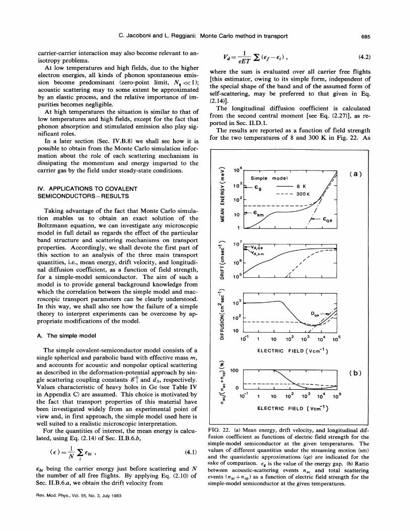
C. Jacoboni and L. Reggiani: Monte Carlo method in transport 685
carrier-carrier interaction may also become relevant to an-isotropy problems.
At low temperatures and high fields, due to the higherelectron energies, all kinds of phonon spontaneous emis-sion become predominant (zero-point limit, Nq « 1);acoustic scattering may to some extent be approximatedby an elastic process, and the relative importance of im-purities becomes negligible.
At high temperatures the situation is similar to that oflow temperatures and high fields, except for the fact thatphonon absorption and stimulated emission also play sig-nificant roles.
In a later section (Sec. IV.B.8) we shall see how it ispossible to obtain from the Monte Carlo simulation infor-mation about the role of each scattering mechanism indissipating the momentum and energy imparted to thecarrier gas by the field under steady-state conditions.
IV. APPLICATIONS TO COVALENTSEMI CONDUCTORS —RESULTS
1Vg= g(Ef —E;),eET
(4.2)
10I)E Simple model
3109
EKLLJ 210LU
(a)
where the sum is evaluated over all carrier free flights[this estimator, owing to its simple form, independent ofthe special shape of the band and of the assumed form ofself-scattering, may be preferred to that given in Eq.(2.14)].
The longitudinal diffusion coefficient is calculatedfrom the second central moment [see Eq. (2.27)], as re-ported in Sec. II.D.1.
The results are reported as a function of field strengthfor the two temperatures of 8 and 300 K in Fig. 22. As
Taking advantage of the fact that Monte Carlo simula-tion enables us to obtain an exact solution of theBoltzmann equation, we can investigate any microscopicmodel in full detail as regards the effect of the particularband structure and scattering mechanisms on transportproperties. Accordingly, we shall devote the first part ofthis section to an analysis of the three main transportquantities, i.e., mean energy, drift velocity, and longitudi-nal diffusion coefficient, as a function of field strength,for a simple-model semiconductor. The aim of such amodel is to provide general background knowledge fromwhich the correlation between the simple model and mac-roscopic transport parameters can be clearly understood.In this way, we shall also see how the failure of a simpletheory to interpret experiments can be overcome by ap-propriate modifications of the model.
A. The simple model
z10
'o10
EO
2Oz 100)
10
10
10
E10
io' I
qe
10 10 10 10 10
(e) =—g cb;,I
(4.1)
eb; being the carrier energy just before scattering and Xthe number of all free flights. By applying Eq. (2.10) ofSec. II.B.6.a, we obtain the drift velocity from
The simple covalent-semiconductor model consists of asingle spherical and parabolic band with effective mass m,and accounts for acoustic and nonpolar optical scatteringas described in the deformation-potential approach by sin-gle scattering coupling constants 8'& and do, respectively.Values characteristic of heavy holes in Ge (see Table IVin Appendix C) are assumed. This choice is motivated bythe fact that transport properties of this material havebeen investigated widely from an experimental point ofview and, in first approach, the simple model used here iswell suited to a realistic microscopic interpretation.
For the quantities of interest, the mean energy is calcu-lated, using Eq. (2.14) of Sec. II.B.6.b,
ELECTRiC F IELD ( Vcm )
100C+
O
c
C
10 1 10 10 10 10 10
ELECTRIC FIELD {Ycm )
FIG. 22. (a) Mean energy, drift velocity, and longitudinal dif-fusion coefficient as functions of electric field strength for thesimple-model semiconductor at the given temperatures. Thevalues of different quantities under the streaming motion (sm)and the quasielastic approximations (qe) are indicated for thesake of comparison. e~ is the value of the energy gap. (b) Ratiobetween acoustic-scattering events n „and total scatteringevents (n„+n,p) as a function of electric field strength for thesimple-model semiconductor at the given temperatures.
Rev. Mod. Phys. , Vol. 55, No. 3, July 1983

686 C. Jacoboni and L. Reggiani: Monte Carlo method in transport
usual, for discussion purposes the electric field range canbe divided into three regions, namely, the linear-responseregion (i.e., E~O), an intermediate region where heatingeffects of carriers become evident, and the highest-fieldregion (i.e., E +a—o,' the comparison between carrier meanenergy and the value of the energy gap of the material setsa physically plausible upper limit on E). To betteranalyze the behavior of different quantities in terms ofsingle microscopic processes, we shall first discuss thelow-temperature (8-K) case.
In the linear-response region E( & 0.2 V/cm in the fig-ure) the following relations hold:
(4.3)
thermore, the drift velocity achieves a new saturation lev-el higher than the previous one, and the diffusion coeffi-cient increases again towards a limiting linear depen-dence. These features are predicted by an analytical solu-tion of the Boltzmann equation with the small anisotropyand quasielastic approximations (Levinson, 196S; Price,1970). This solution, which well applies to the highest-field region (E) 10 V/cm in the figure), considers onlyoptical-phonon enussion processes and leads to the fol-lowing relations:
(4.9)
(4.4) Vd = 2 Kg8,377m
(4.10)
pKg TpD=e
(4.S) EDI ——vd lop (4.1 1)
The above equations, which are usually referred to asequipartition of energy, Ohm s law, and the Einstein dif-fusion relation, respectively, are well reproduced byMonte Carlo results at the lowest field strengths [see Fig.22(a)].
The intermediate region starts at about 1 V/cm, and upto about 10 V/cm the acoustic scattering mechanism isthe only active one [see Fig. 22(b)]. Owing to the quasie-lastic nature of this mechansim the mean energy is foundto increase and the diffusion coefficient to increase slight-ly above its thermal equilibrium value. Furthermore,since the scattering efficiency of acoustic modes increaseswith electron energy (see Sec. III.D.l.d), the drift velocityis found to behave in a sublinear way.
In the region of field strengths between 10 and 10V/cm, the optical scattering mechanism builds up until itpredominates over acoustic scattering [see Fig. 22(a)].The strong optical emission process prevents furtherstrong heating, so that the mean energy attains an approx-imately constant value, the drift velocity tends to saturate,and the diffusion coefficient decreases. These featuresfollow what is predicted by the streaming motion approx-imation, which at this temperature well applies to thefield range and for which simple theoretical considera-tions lead to the relations
Here E, is a critical field given by
3 m
2meka p(4.12)
which, under E/E, & 1, well justifies the above asymptot-ic solution; I,p is the mean free path due to optical-phonon scattering given by
(4.13)
B. Real-model applications
The asymptotic prediction of Eqs. (4.9)—(4.11), whichwithin statistical uncertainty are found to agree withMonte Carlo calculations, are reported in Fig. 22(a).
In the high-temperature case (To ——300 K), owing tothe increased efficiency of the scattering mechanisms indissipating to the lattice the energy gained by the field,the region of field strengths for which the linear-responseregion holds is extended (E &10 V/cm in the figure).Owing to the increased importance of acoustic-phononscattering and the optical absorption process, thestreaming-motion region disappears, and at the highest-field region (E& 10 V/cm) the results are no longer inclose agreement with those of Eqs. (4.9)—(4.11).
1/2EgO, p
2m(4.7)
DI ——0. (4.8)
The limiting values given by Eqs. (4.6) and (4.7) are re-ported with Monte Carlo results in Fig. 22(a) for the sakeof comparison.
In the region of field strengths above 10 V/cm, the op-tical scattering mechanism keeps its predominant role, butis no longer able to fully dissipate the energy gained bythe carriers from the field. As a consequence the carriermean energy is found to increase more and more steeplywith field toward a limiting quadratic dependence; fur-
The simple model represents too crude a simplificationto offer any deep microscopic physical insights or to per-mit a quantitative comparison between theory and experi-ments. Consequently, in the following we present a sur-vey of the more significant results which, in our opinion,have been obtained for elemental semiconductors of groupfour when full details of the band structure and scatteringmechanisms are taken into account.
1. Drift velocity
Methods for calculating the drift velocity have been re-ported in See. II.B.6. Usually this quantity is investigatedfor the material of interest at given temperatures as a
Rev. Mod. Phys. , Vol. 55, No. 3, July 1983

C. Jacoboni and L. Reggiani: Monte Carlo method in transport 687
10 =7~
(~ I ~ 1
I
I I 1I
I 1 I I
~ O ~0
I I II
I I III I & II
I I ~ I
„O~OS~&I I I
II I ll
710
O
EV
I—C30LU
0
610xV'
106
04 olIL710
107
10 Si holes4 ~ 4 &111 &
o o o &100&
10 10I I I I I IIII I I II
1010 10 103 10
EL E CT RIG F IE L D (V cm ')FIG. 23. Drift velocity as a function of electric field strengthfor holes in Si at the given temperatures. Points refer to experi-ments and curves to theoretical Monte Carlo calculations (Reg-giani, 1980).
function of electric field strength applied along differentcrystallographic directions.
Figure 23 shows a set of results for the case of holes inSi (Ottaviani et al. , 1975; Reggiani, 1980). Here the an-isotropy of the drift velocity with field orientation, whichoccurs at high field strength, reflects the warped shape ofthe equienergetic surfaces of heavy holes. Furthermore,at 6 K a peculiar effect of a near-saturation region at in-termediate fields (50&E &200 V/cm) is interpreted as anonparabolic effect of the band (Canali et al. , 1973).
Figure 24 shows a set of results for the case of electronsin Ge (Jacoboni et a/. , 198la). In this case the drift velo-city exhibits anisotropic effects due to the many-valleystructure of the conduction band. Furthermore, the pres-ence of higher minima, lying a few hundred meV abovethe conduction-band minimum, makes possible scatteringto higher minima. Thus, in order to be realistic, the mi-croscopic model should include four equivalent absoluteminima located at 1. points, one upper minimum locatedat the I point, and six further minima higher than the j.one, located along b. The presence of these upper mini-ma, together with nonparabolicity, is found to be the
I II
I I I I I I[
I I I I
710 :107
10OICO
—10
O
«~~~ ex pt &1710 = oo "expt &1
O : theor &
UJ ---- theor &
13
—10
10' 7:10
6:1
1 10 10 10ELEGTRIG FIELD (V om")
FKx. 24. Drift velocity as a function of electric field strength for electrons in Cxe at the given temperatures. Circles and triangles
refer to experiments performed at the two concentrations of electrons reported. Curves refer to theoretical Monte Carlo calculations
(Jacoboni et a/. , 1981a).
Rev. Mod. Phys. , Vol. 55, No. 3, July 1983

C. Jacoboni and L. Reggiani: Monte Carlo method in transport
I ] Il
f i/Ii I I Il
& &I I
(
I i &
l I ll 4
VQ)M
EU
O 5(g 10M
E4
10
]0 310 l i i i l
sinai
1 10 10 10
10'10 10
TEMPERATURE (K)FIG. 25 ~ Mobility of holes in Ge as a function of temperature.Different points refer to experiments: dashed curve, MonteCarlo theoretical results in the parabolic case; solid curve,Monte Carlo results when nonparabolic effects are taken intoaccount (Reggiani et al., 1977).
FIG. 26. Mobility of electrons in Si as a function of tempera-ture. Different points refer to experiments: solid curve,theoretical results when lattice scattering only is considered;dot-dashed curve, theoretical results with lattice scattering plusionized impurity scattering with nI ——10" cm ' (Canali et al.,1975).
tocorrelation function in the absence of a field (Gherardiet al. , 1975). This quantity is related to the electron mo-bility by
source of a negative differential mobility region which oc-curs at the highest field strengths for the case of low tem-perature (To & 77 K). It is worth noting that experimentsgive evidence of a dependence of the drift velocity alongthe (111) direction upon electron concentration, that is,upon electron-electron scattering, which has not yet beenfully interpreted (Jacoboni, 1976).
2. Ohmic mobility
In order to find the Ohmic mobility at a given tempera-ture by Monte Carlo simulation, one can calculate the ra-tio vd/E for a set of field values low enough to verify theindependence of this ratio from field strength (the con-comitant tendency to the equilibrium value of the meanenergy provides a good check). Figure 25 shows the re-sults of such a calculation for the case of holes in Ge(Reggiani et al. , 1977). It must be noted that inclusion ofnonparabolicity effects in the theoretical model slightlylowers the mobility values at higher temperatures withrespect to the parabolic case (dashed curve in Fig. 25).
However, as indicated in Sec. II.E, a more appropriateprocedure consists of evaluating the diffusion coefficientat zero field; then the mobility is obtained from the Ein-stein relation [see Eq. (4.5)]. Figure 26 shows results ob-tained for the case of electrons in Si (Canali et al. , 1975).Here the dashed-dotted curve refers to the case for whichimpurity scattering with a concentration of 10 cm isincluded.
The diffusion coefficient method can be applied bymeans of a direct simulation of the integrated velocity au-
p= f C(r)dr .Kg Tp
(4.14)
Figures 27 and 28 show the results of such a calculationfor the case of electrons in Si when only acoustic scatter-ing is carried out in an exact approach. Figure 27 showsthe mobility obtained at different temperatures as a func-
I & I l f l l l
)
O(D
EO
10
10
~~ ~ e —e —e~ ~
e/
Ie
~~ e —e —e —e —e —e —~ —ee
e—~—e —e-e —e-~ -e-ee
CQ
Oe-e-e-e-e —e-e-e —~ —e 4 5
e—~-e-e —e-~ -e —e —e -e 77
410 ( r l l l l l I
0 2 4 6 8 10
COR RELATED FLIGHTS
FIG. 27. Mobility of electrons in Si as a function of correlatedflights at the indicated temperatures (Gherardi et al., 1975).
Rev. Mod. Phys. , Vol. 55, No. 3, July 1983

C. Jacoboni and L. Reggiani: Monte Carlo method in transport 689
tion of the number of correlated flights. It can be seenthat the assumption of totally randomizing scattering,which corresponds to a flat curve in Fig. 27, is justifiedfor temperatures around and above 45 K. Furthermore,as a result of avoiding the usual elastic and energyequipartition approximations, below about 45 K the mo-bility is found to increase more rapidly over the well-known result p cc To (see Fig. 28).
10
IoIEo 10
I I I l I I I I I I i I I I I I I I I I
10
3. Diffusion
The method for calculating the diffusion coefficienthas been discussed in Sec. II.D. It is worth noting thatthe Monte Carlo technique first provided an exact calcu-lation of diffusion. As in the case of drift velocity, atgiven temperatures this quantity is investigated as a func-tion of electric field strength for different crystallographicdirections.
Figure 29 shows a set of results for the case of holes inSi (Navi et al. , 1979; Reggiani, 1980). Here the anisotro-
py of the longitudinal diffusion coefficient again reflectsthe warped shape of the equienergetic surfaces of heavyholes. Furthermore, the tendency to saturate at thehighest field strengths is ascribed to nonparabolicity ef-fects of the heavy-hole band.
Figure 30 shows a set of results for the case of electronsin Si (Brunetti et al., 1981). Here the anisotropy of the
10
1
10
~ ~ ~Lhk
ooo --—&100 &
l. . . , I
10l I IIIl
10'E (Vcm ')
FIG. 29. Longitudinal diffusion coefficient of holes in Si as afunction of electric field strength at the given temperatures.Points refer to experiments and curves to theoretical MonteCarlo calculations (Reggiani, 1980).
longitudinal diffusion coefficient with respect to theorientation of the field in the crystal is related to an addi-tional intervalley diffusion which arises owing to the factthat, when the field is oriented along a (100) direction,electrons exhibit different mean velocities in different val-leys. In addition, the microscopic simulation enables usto compare the magnitudes of the transverse and longitu-dinal diffusion coefficients [DI/Dt) 1 in this case, con-trary to results obtained by analytical calculations (Perskyand Bartelink, 1970), which is to be explained in terms ofthe energy dependence of the scattering probability]. InFig. 31 the electron mean energy (continuous line) and the
10llll I I I ) lllll I I I /l Illf
3Si electrons vol
ool&100 &
l l
10
4410 10 2
Kl 10— V
M
E
10 2
160 K
10
10102
QB- -Q
3&o I I I I I s I I l
10 10
200 K
10Hill I l l I ««l « I I I l»l
10 10 10
10I ) lllll
10
TEMPERATURE ( K) E (Vcm')
FIG. 28. Mobility of electrons in Si as a function of tempera-ture, obtained with the simulated velocity autocorrelation func-tion (solid curve), compared with the traditional result p ~ To(dashed curve) (Gherardi et aI., 1975).
FIG. 30. Longitudinal diffusion coefficient of electrons in Si asa function of electric field strength at the given temperatures.Points refer to experiments and curves to theoretical MonteCarlo calculations (Brunetti et al., 1981).
Rev. Mod. Phys. , Vol. 55, No. 3, July 1983

690 C. Jacoboni and L. Reggiani: Monte Carlo method in transport
1500
hC
1000IX
500X
I
Si electrons
300- K
E = ~0 kV/cmf ll &111&
mean energynumber of electrons
III
I
~ JI
r~lI
II
L~II
III
I
II
L~IL
I
L
150
(0
0100
050
XD
independent of position. In contrast, along the directionof the field, electrons in the front of the cloud havegained more energy from the field and thus have a meanenergy higher than electrons in the rear. Since thescattering probability increases with energy, it will behigher for the front electrons (and the mobility lower)than for rear electrons, and consequently the cloud willexpand less than in the homogeneous transverse case.
4. Mean energy
1500
1000CL'
500
0-50
I
II
L
II
I
I
I
L
IL
I
II
0
POSITION (io cm)50
150
M
Q
100
050
IXI
number of electrons (dashed line) are shown as a functionof electron position in the cloud along [see Fig. 31(a)] andperpendicular to [see Fig. 31(b)] the field, oriented along a(111) direction. Along a direction orthogonal to thefield the mean energy is, apart from random fluctuations,
FIG. 31. Mean energy {solid curve and left scale) and numberof electrons {dashed curve and right scale) as a function of posi-tion for the case of electrons in Si: (a) longitudinal direction; (b)transverse direction. The simulation time is 2.2&(10 ' sec foran initial spatial distribution of the Dirac type {Brunetti et al. ,1981).
A method of calculating the mean energy is given byEq. (4.1) or by the adaptation of Eq. (2.10) to the case ofenergy. Figure 32 shows the results for the case of elec-trons in Ge (Jacoboni et al. , 1981a). At 8 K the mean en-
ergy exhibits an initial rise due to the dominant contribu-tion of the acoustic scattering mechanism, then a nearlyconstant region shows up at intermediate field strengthsowing to the buildup of intervalley phonon emission, asexpected from the simple model. At the highest fieldstrengths the mean energy does not exhibit the E asymp-totic tendency, as found in the simple model, as an effectof nonparabolicity of the band and because the scatteringto upper valleys gives rise to additional dissipationmechanisms which combine to moderate the heating ofthe electron gas (Fawcett and Paige, 1971). It is worthnoting that at field strengths as high as 10 V/cm themean energy keeps values lower than the energy gap (0.66eV at 300 K).
From these curves, by analyzing the departure fromthermal equilibrium, one can evaluate the region of fieldstrengths at which hot-electron effects are expected to be-gin at a given temperature; as a general trend, it is foundthat this region starts at higher fields for higher tempera-tures. The knowledge of the mean energy as a function offield can be of special value when a rough estimate ofbreakdown fields of bulk devices is desired.
I I lI I I I
(I I I
II I I I
jI I I
f 1 I It[ I I I l I I
106 e electrons
E II &100&
-210
1010
I IIl10 10 10
ELECTRIC FIELD (Vcm ')I
10
FJG. 32. Mean energy of electrons in the lower valleys of Ge as a function of electric field strength at the given temperatures.
Rev. Mod. Phys. , Vol. 55, No. 3, July 1983
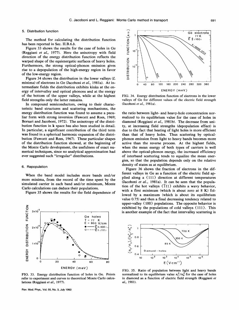
C. Jacoboni and L. Reggiani: Monte Carlo method in transport 691
5. Distribution function
6. Repopulation
When the band model includes more bands and/ormore minima, from the record of the time spent by thesimulated carrier in each band and/or minimum, MonteCarlo calculations can deduce their populations.
Figure 35 shows the results for the field dependence of
D -33x10
C3
LL
Z -32x10
I—
KlCY
-31 x10
Cl
6 e holesT=77 K
The method for calculating the distribution functionhas been reported in Sec. II.B.6.b.
Figure 33 shows the results for the case of holes in Ge(Reggiani et al., 1977). Here the anisotropy with fielddirection of the energy distribution function reflects thewarped shape of the equienergetic surfaces of heavy holes.Furthermore, the strong optical-phonon emission givesrise to a depopulation of the high-energy region in favorof the low-energy region.
Figure 34 shows the distribution in the lower valleys (Lminima) of electrons in Ge (Jacoboni et al., 1981a). At in-termediate fields the distribution exhibits kinks at the en-
ergy of intervalley and optical phonons and at the energyof the bottom of the upper valleys, while at the highestfield strengths only the latter remains.
In compound semiconductors, owing to their charac-teristic band structures and scattering mechanisms, theenergy distribution function was found to assume a pecu-liar form with strong inversion (Fawcett and Rees, 1969;Borsari and Jacoboni, 1972). The anisotropy of the distri-bution function in k space has also been studied in detail.In particular, a significant contribution of the third termwas found in a spherical harmonic expansion of the distri-bution (Fawcett and Rees, 1967). These particular shapesof the distribution function showed, at the beginning ofthe Monte Carlo development, the usefulness of exact nu-merical techniques, since no analytical approximation hadever suggested such "irregular" distributions.
GJ
Z',
O
10
I I I I6e elect rons
D
10Kl
I—ICi
the ratio between light- and heavy-hole concentration nor-malized to its equilibrium value for the case of holes indiamond (Reggiani et al., 1981b). The decrease from uni-ty, at increasing field strengths (depopulation effect) isdue to the fact that heating of light holes is more efficientthan that of heavy holes. Thus scattering by optical-phonon emission from light to heavy bands becomes moreactive than the reverse process. At the highest fields,when the mean energy of both types of carriers is wellabove the optical-phonon energy, the increased efficiencyof interband scattering tends to equalize the mean ener-gies, so that the population depends only on the relativedensity of states as at equilibrium.
Figure 36 shows the fraction of electrons in the dif-ferent valleys in Ge as a function of the electric field ap-plied along a (111) direction at different temperatures(Jacoboni et al. , 1981a). It can be seen that the popula-tion of the hot valleys (111) exhibits a wavy behavior,with a first minimum (which is about zero at 8 K) fol-lowed by a maximum (which is about its equilibriumvalue 0.75) and then a final decreasing tendency related toupper-valley (100) populations. The opposite behavior isexhibited by the populations of cold valleys (111). Thisis another example of the fact that intervalley scattering is
a
O ~40.8
o.6
Diamond —holes
0 40 80 120 160 200 240 280 320 360
ENERGY (meV)
FIG. 34. Energy distribution function of electrons in the lowervalleys of Ge for different values of the electric field strength(Jacoboni et al., 1981a).
0.410
I
10 10I
10I
10I
1020 40 60 80 E(Vcm ')
ENERGY (meV)
FIG. 33. Energy distribution function of holes in Ge. Pointsrefer to experiment and curves to theoretical Monte Carlo calcu-lations (Reggiani et al., 1977).
FIG. 35. Ratio of population between light and heavy bandsnormalized to its equilibrium value n~ /nq for the case of holesin diamond as a function of electric field strength (Reggiani etal., 1981).
Rev. Mod. Phys. , Vol. 55, No. 3, July 1983

692
0
60C)
I I lI IIII I I I I' I''IIIII I I I l I IIII I
Ge elect ron sS i e I ect rons8 K
E II & 111& 77 K&111 & w &1 11&
0LLJ
4QZ,'
0I—
X
20CL
0.8
0.6
0.4
0.2(Dz00
1 0
I~ ~
I $ ~ 1 ~ I I I~ ~ 1I
I
~ I I
Ge elec trons
(3CC
0
20 K
E II «»&+ +0
0T I
&111&+ &111 &
1.0 1.5 2.00.2 Q.4u 080ELECTRIC FIELD ( k V cm ")
FIG. 37. Energy relaxation time of electrons in Si as a functionof electric field strength. Points refer to experiments, curves totheoretical Monte Carlo calculations (Jacoboni, 1976).
0.6Z'
0.4
0.2
~ ~ q ~~ sr ~
II ~ ~
I~ ~ ~ ~
II I I i ~ I I ~
Ge elect ron s
from the Monte Carlo simulation, we obtain a theoreticalevaluation of ~, .
Monte Carlo results for electrons in Si (Jacoboni, 1976)are shown in Fig. 37, which reports the results of ~, as afunction of electric field strength, and in Fig. 38, whichreports the results of ~, as a function of temperature.The decrease of ~, with an increase in either E or To hasthe same physical origin: when electron energies are in-creased, intervalley phonons become more effective in dis-sipating energy.
45 K
E &111 &
&111&+ &111&1.0
0.8
0.6
0.4
0. 2
101010 10
EL ECTR IC F IE LD (V cm ) 8. Efficiency of scattering mechanismsFICx. 36. Population of the different valleys as a function ofelectric field strength for the case of electrons in Ge at the giventemperatures. Points indicate experimental results, curvestheoretical Monte Carlo calculations (Jacoboni et al., 1981a).
The efficiency of a scattering inechanism is measured
by its energy and momentum dissipation rate. By collect-
O&i)M
CU
0inore probable for electrons in hot valleys, thus bringingabout repopulation. The total effect is reduced as thetemperature increases, since in this case the difference inenergy between hot and cold valleys is reduced.
102
O
OC
UJCC
7. Energy relaxation time
10The energy relaxation time, which should describe in a
phenomenological way the tendency of the isotropic partof the distribution function to decay toward its equilibri-um value, is defined by (see the textbook of Seeger, 1973)
Si electrons
&~ &—&~0&
UdeE
50 100 150(4.15)
T E IVI P E R A T U R E ( K)
where (eo) is the thermal-equilibriuin mean energy of thecarriers, and (e ) is the mean energy in the presence of afield. By substituting for (e) and Ud the values obtained
FICx. 38. Low-field energy relaxation time of electrons in Si asa function of temperature. Points refer to experiments, thecurve to theoretical Monte Carlo calculations (Jacoboni, 1976).
Rev. Mod. Phys. , Vol. 55, No. 3, July 1983
C. Jacoboni and L. Reggiani: Monte Carlo method in transport

C. Jacoboni and L. Reggiani: Monte Carlo method in transport 693
OIO
UJ
10 ~ &
l& & I I
Ge elE ll&~
0" —77 K
I I Il
I & IIi t I & IVI I I / I /I I
109
ing for each type of scattering the amount of energy andmomentum dissipated at the scattering events, one canevaluate these efficiencies in the Monte Carlo simulation.
Figure 39 shows the energy (a) and momentum (b) dis-sipation rates for all scattering mechanisms considered inthe lower valleys for electrons in Ge (Jacoboni et al.,1981a). At the temperature considered, acoustic scatter-ing is dominant at low fields for momentum dissipation,but negligible for energy dissipation, which is ensured byoptical and equivalent interv alley scattering. At thehighest fields, nonequivalent intervalley scattering is themost important means for dissipating both energy andmomentum. Let us note that the results reported here al-ready include a reduction in efficiency due to valley de-
population at high fields, since the dissipation rates havebeen evaluated by dividing the dissipated quantity of in-terest by the total simulation time.
9. White noise
Monte Carlo calculations of the noise spectrum of thevelocity fluctuations S„as obtained by Fouriertransforming the velocity autocorrelation function [seeEq. (2.41)], are shown in Fig. 40 for the case of electronsin Si (Brunetti, 1982). At low frequency the well-knownwhite spectrum is exhibited; the transverse component isfound to be larger than the longitudinal one, in accordwith a D, &Dl [see Eq. (2.42)]. At the highest frequen-cies, structures appear in the longitudinal case which canbe correlated with the characteristic intervalley scatteringtime, while the transverse case exhibits only simpleLorentzian decay.
An interesting comparison of Monte Carlo results withnoise experiments can be carried out under the followingconditions. When a two-terminal device exhibits a posi-tive value of the real small-signal impedance Re(W), andcarrier-carrier scattering is neglected, the equivalent noisetemperature associated with velocity fluctuations (white-noise temperature) T„ is given by (Shockley, 1966; VanVliet et al. , 1975; Nougier et a/. , 1981)
108gE 2
K~ Re[%(E)]
10
104
Ge(D
1Q 77IX
I I I ) IIII I I I I I I&l
n r 7', r,ED EV', r,Edr,
I Il
I [ I II I I I II I I II
(4.16)
where r&t', N(r, E) is the impedance field and the integra-tion is performed over the volume of ihe device V.
Provided the geometry and doping of the device are
10
S i ele
10
LLI
C)1
10 10 10 10 10'
300 K
E= 50E ) &111
I
1 O1 21 O13 1 014
ELECTRIC FIELD (V cm )
FICz. 39. Energy (a) and momentum (b) dissipation rates for thecase of electrons in Ge due to the various scattering mechanismsin the lower valleys as functions of electric field strength: AC,acoustic; OP, optical; IE, intervalley between equivalent mini-ma; I, intervalley between nonequivalent minima (Jacoboni etal., 1981a).
(sec ")FIG. 40. Noise spectrum of the velocity fluctuations as a func-tion of angular frequency for the case of electrons in Si: solidcurve, longitudinal component; dot-dashed curve, transverse
component; dashed curves at lowest frequencies are extrapola-tions to the zero-frequency values of S,. The Lorentzian decayas co is shown for the sake of comparison.
Rev. Mod. Phys. , Vol. 55, No. 3, July 1983
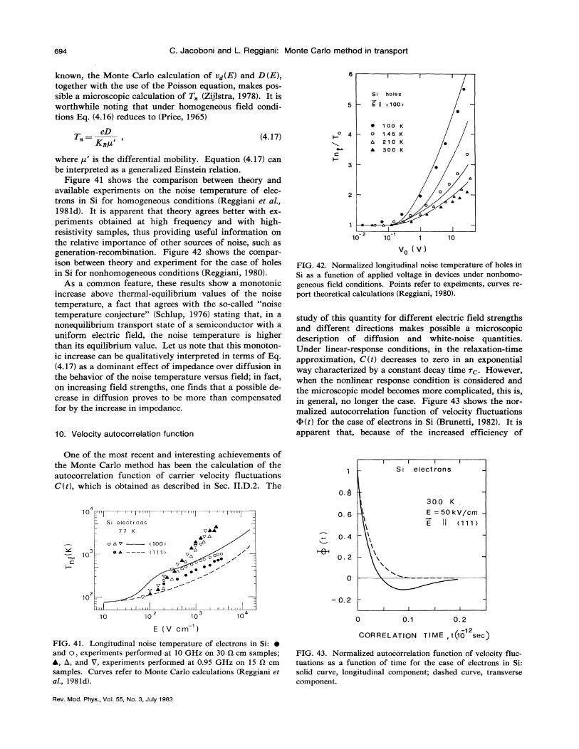
694 C. Jacoboni and L. Reggiani: Monte Carlo method in transport
known, the Monte Carlo calculation of Ud(E) and D(E),together with the use of the Poisson equation, makes pos-sible a microscopic calculation of T„(Zijlstra, 1978). It isworthwhile noting that under homogeneous field condi-tions Eq. (4.16) reduces to (Price, 1965)
Si h
5 — E II
eDTn gK~p'
(4.17)0
~ 100 1 4
2130
where p is the differential mobility. Equation (4.17) canbe interpreted as a generalized Einstein relation.
Figure 4jL shows the comparison between theory andavailable experiments on the noise temperature of elec-trons in Si for homogeneous conditions (Reggiani et al.,1981d). It is apparent that theory agrees better with ex-periments obtained at high frequency and with high-resistivity samples, thus providing useful information onthe relative importance of other sources of noise, such asgeneration-recombination. Figure 42 shows the compar-ison between theory and experiment for the case of holesin Si for nonhomogeneous conditions (Reggiani, 1980).
As a common feature, these results show a monotonicincrease above thermal-equilibrium values of the noisetemperature, a fact that agrees with the so-called "noisetemperature conjecture" (Schlup, 1976) stating that, in anonequilibrium transport state of a semiconductor with auniform electric field, the noise temperature is higherthan its equilibrium value. Let us note that this monoton-ic increase can be qualitatively interpreted in terms of Eq.(4.17) as a dominant effect of impedance over diffusion inthe behavior of the noise temperature versus field; in fact,on increasing field strengths, one finds that a possible de-crease in diffusion proves to be more than compensatedfor by the increase in impedance.
10. Velocity autocorrelation function
10
II
10f
1
v, (vj10
FIG. 42. Normalized longitudinal noise temperature of holes in
Si as a function of apphed voltage in devices under nonhomo-
geneous field conditions. Points refer to expeiments, curves re-
port theoretical calculations (Reggiani, 1980).
study of this quantity for different electric field strengthsand different directions makes possible a microscopicdescription of diffusion and white-noise quantities.Under linear-response conditions, in the relaxation-timeapproximation, C(t) decreases to zero in an exponentialway characterized by a constant decay time ~~. However,when the nonlinear response condition is considered andthe microscopic model becomes more complicated, this is,in general, no longer the case. Figure 43 shows the nor-malized autocorrelation function of velocity fluctuationsN(t) for the case of electrons in Si (Brunetti, 1982). It isapparent that, because of the increased efficiency of
One of the most recent and interesting achievements ofthe Monte Carlo method has been the calculation of theautocorrelation function of carrier velocity fluctuationsC(t), which is obtained as described in Sec. II.D.2. The
o. a
I 1
S i elect rons
1 0Si electr ons
I I Ii
I I I I[ I I Ii
I I II] 0. 6
0. 4
300 K
E =50kV/cm—E II &)1& I
10 0. 2
102
10 10 10 10 0.1 0.2E (V clTI )
FIG. 41. Longitudinal noise temperature of electrons in Si:and O, experiments performed at 10 GHz on 30 Q cm samples;4, 5, and V, experiments performed at 0.95 GHz on 15 0, cmsamples. Curves refer to Monte Carlo calculations (Reggiani etal., 198ld).
-12CORRELATION T IME, t(10 sec)
FIG. 43. Normalized autocorrelation function of velocity Auc-tuations as a function of time for the case of electrons in Si:solid curve, longitudinal component; dashed curve, transversecomponent.
Rev. Mod. Phys. , Yol. 55, No. 3, JUly 1983

C. Jacoboni and L. Reggiani: Monte Carlo method in transport 695
scattering, for the high-field case 4(t) decreases to zerofaster, the transverse component being larger than thelongitudinal one, in agreement with a D, & DI.
Figure 44 shows a set of curves for the longitudinal@(t) when the field is along the &100) and (111) direc-tions. The peculiar negative behavior exhibited by @(t) inthis figure is correlated with long flights in k space,characterized by initial negative velocity fluctuationswhich carriers can undergo after an intervalley scattering.
11. Alternating electric fields
The application of the Monte Carlo technique to thecase of periodic fields has been reported in Sec. II.C.3.
Figure 45 shows the real and imaginary parts of thedifferential inobility as a function of frequency for thecase of electrons in Si, when the static electric field is 10and 50 kVlcm, respectively (Zimmermann et al., 1978).The real part of the mobility at the lower frequency coin-cides with the differential mobility at the bias point; then,with increasing frequency, it peaks and finally tends tozero. This is a general feature of the frequency depen-dence of all transport phenomena when a strong scatter-ing process with a threshold energy determines an oscilla-tory behavior of charge carriers. Recalling that the opti-cal absorption coefficient of free charge carriers is pro-portional to the small signal conductivity, this peakrepresents a resonant absorption at the corresponding fre-quency. The imaginary part of the mobility, which isknown to give the free-carrier contribution to the dielec-tric constant, has the frequency dependence predicted byKramers-Kronig relations (Zimmermann et al., 1978).
12. Magnetic fields
The method of introducing a magnetic field in MonteCarlo calculations has been reported in Sec. II.F. Quite
I O 800 I I
Si elect rons600)400
CJ
200I—
0CQ
OE =10 kV/cm~vE = 50 kV/cm
200
0CLLULl —200Li
C5 —4pp i ii, l
10 10j I I I I I I
10
interesting results have been obtained under streaming-motion conditions (Maeda and Kurosawa, 1972; Andro-nov et al., 1980; Kurosawa, 1980). For a simple-modelsemiconductor, the simultaneous presence of a streamingmotion and of a circular inotion with a frequencyco, =eB/(mc) gives rise to an accumulation region in kspace, which assumes a spindle shape (see Fig. 46). Thiseffect is easily understood by considering the differentbehavior of a carrier depending on its initial conditions ofmotion immediately after optical-phonon einission. If thecarrier is outside the accumulation region, it is shortlived, since it will be accelerated up to energies larger thanfico,~ within a short time (of the order of co, '). If thecarrier is inside the accumulation region it is long lived,since the circular motion continues for a long time. As aconsequence, the energy distribution function shows apopulation inversion reflecting the strong accumulation in
FREQUENCY (G Hz)
FIG. 45. Real (a) and imaginary (b) part of the differential mo-bility of electrons in Si as a function of frequency at the fieldstrengths reported (Zirnmermann, 1978).
0.8
0.6&111)&1PP)
z„B ' "z
0.4
0 ~ 2ky
—0.2
0.1 0 ~ 2 0.3 kx
CORRELATION TiME, t (]o sec)
FIG. 44. Normalized autocorrelation function of longitudinalvelocity fluctuations as a- function of time for the case of elec-trons in Si: solid curves, electric field along the (111) axis;dashed curves, electric field along the ( 100) axis.
FIG. 46. Carrier motion in k space under an electric field Eand a magnetic field 8 perpendicular to E. Spindle region is la-beled S; the dashed line represents the axis of the spindle regionand crosses the center point at C [0, mcE/( AB),0]. f—m,„ isthe energy of the optical phonon (Maeda and Kurosama, 1972).
Rev. Mod. Phys. , Vol. 55, No. 3, July 1983

C. Jacoboni and L. Reggiani: Monte Carlo method in transport
( Fig. 47). These predictions havebeen experimentally confirmed for the case of holes in Cie
by Komiyama and Spies (1981).
I
Sl elect ron s300 K
E ll (100&
13. Transients
The method of calculating time-dependent phenomena(under transient conditions) has been described in Sec.II.C.1. Figure 48 shows Monte Carlo calculations for t ecase of electrons in Si with given initial conditions ofmotion (Reggiani et al., 1981a). The main features of theresults are the tendency of the drift velocity and diffu-
xceed their value at long times for a brief periodof time (overshoot effects).
Figure 49 shows results for the case of holes in Si (Reg-1 1981b). Here the transient behavior of thegiani et a.,
drift velocity and mean energy is investigated at i erenFi . 49(a) theinitial energies. As can be seen in Fig. &a, e
overshoot is maximum for the coldest initial distribution,while it disappears for the hottest case. This phenomenonreflects the energy dependence of the momentum relaxa-tion time, as discussed m Sec. II.B.2 (see 'g.Fi . 2). In otherwords, when carriers start with a low energy, they beginto accelerate before dissipating energy, and, provided thefield strength is high enough, they have the possibility onaverage of reaching velocity values higher than the sta-tionary ones. If the carriers start with high energies, theysimultaneously start accelerating and dissipating energythrough phonon emission; this fact leads to a smooth in-crease with time of the drift velocity, so that overshoot ef-fects are not present.
As regards the transient energy [see Fig. 49(b)] noovershoot is observed.
C. Devices
Th M nte Carlo method is finding fruitful apphca-leh rea of modeling real devices (see for examp e
Constant and Boittiaux, 1981). As explained in the Intro-duction, t is opic is nh t is not within the scope of this review;
I0, /
30
IUzo—
CU
E10
Cl
—-- E =20 kV/cmE = 100 k V/cm
(b)Q 5 1
TIME (10 sec )
however, owing o i st 'ts practical importance, in this sectionwe shall briefly outline the main objectives of such a useand summarize some interesting applications that haveappeared in the literature.
When the dimensions of devices become very small
IUQ
EV
CO
C)"0.5LLl
1.0 — r)/
I
S i holes300 K
50 kVjcrn
~ 0FIG. 48. Drift velocity (a) and longitudinal diffusion coefficient(b) as functions of time for the case of electrons in Si. The ini-tial conditions o mo ion ad
' f tion are taken with all carriers starting3from the same point (x =0) at fixed energy equal to (&
) KgTpwith k orthogonal to E.
Ge holes8.6 K
20 kQe
10 =LU
(C&0
03
eTO
0.75 ev
0 'fl ~o 6FIG. 47. Energy distribution function of holes in Cie for thegeometry of fields in Fig. 46: (a) electric field strength of 2.5kV/cm; (b) electric field strength of 3 kV/cm; (c) electric fieldstrength of 3.25 kV/cm. Energies eI. and e~ correspond to
I and C in Fig. 46, and Ace p is the optical-phonon ener-gy (Maeda and Kurosawa, 1972).
/
/
I10 /
0 0.5
TIME (]o sec)FIG. 49. Drift velocity (a) and mean energy (b) as functions oftime for the case of holes in Si. Different curves refer to the re-ported different values of the initial mean energy with velocityrandomly distributed (Reggiani et aL, 198I).
Rev. Mod. Phys. , Vol. 55, No. 3, July 1983
C. Jacoboni and L. Reggiani: Monte Carlo method in transport 697
(submicron devices) and the frequencies of the appliedfields very high (over 10 GHz), classical phenomenologi-cal transport equations are no longer adequate to describecharge current, and a direct solution of the kinetic equa-tion has to be undertaken (Rees, 1973). Under the aboveconditions, the Monte Carlo method becomes a powerfultool for modeling devices. The major remaining problemis to describe in a self-consistent way the spatial depen-dence of the field inside the crystal.
Interesting applications of Monte Carlo to devicemodeling have already appeared in the literature.Domain formation in Gunn devices has been analyzed byLebwohl and Price (1971b). The Gunn effect in fer-romagnetic semiconductors has been studied by Aerset al. (1976). The transport of carriers across the base ofa Si, narrow-base, bipolar transistor has been investigatedby Baccarani et al. (1977). The high-field drift velocityof carriers in the p- and n-channel inversion layers of Sihas been reported by Basu (1977) and Zimmerinann et al.(1980). Unipolar components for both diffusion noiseproperties and static characteristics have been investigatedby Zimmermann and Constant (1980). The simulation ofreal-space electron transfer in GaAs-AIGaAs heterostruc-tures has been carried out by Glisson et al. (1980).
V. CONCLUSIONS
In the last decade Monte Carlo, by making possible theuse of sophisticated microscopic models for both bandstructure and scattering mechanisms of any material, hasproved to be an extremely powerful method for the studyof transport phenomena in semiconductors.
In particular, this method has provided a detailed phys-ical interpretation of the response of a semiconductor toarbitrary fields. Mobility and diffusivity have been themain objects of investigation, but many other particularfeatures of the transport process have been elucidated inMonte Carlo simulations, such as, for example, space,velocity, and energy distributions, valley repopulations,efficiencies of scattering mechanisms, fluctuations, and soon. In this respect the method has become a sort of simu-lated experimental technique with very strong insight po-tentiality, through which experimentalists belonging todifferent areas have found a unifying theoretical methodfor understanding the physics that underlies their results.Some features of the Monte Carlo technique have beentaken to a high level of refinement, such as, for example,the use of the entire conduction band instead of theeffective-mass approximation (Shichijo and Hess, 1981).On the other hand, one problem that still requires a defin-itive clarification is the best way for the generalization ofthe model to include electron-electron interaction.
The feasibility of the Monte Carlo method is such thatalmost all the areas where it could be applied have beeninvestigated in a relatively short time, so that it is nowreasonable to think of its extension to new areas which arebecoming ripe for deeper investigation. The transportproperties of new physical systems —for example, quasi-
one-dimensional structures, intercalation compounds, aLdamorphous materials —will be profitably studied bymeans of the Monte Carlo technique as soon as their basicphysical properties are well enough understood for theconstruction of realistic and reliable models to be used inthe simulation. A similar consideration holds for devicedesign where, however, a further difficulty arises from theneed to know the field distribution inside the device itself.In this case a self-consistent calculation must be per-formed. When submicron structures are involved, directsimulation seems to be the only feasible approach to de-vice analysis.
A major field that, presumably, will benefit significant-ly by application of the Monte Carlo technique is quan-tum transport (Barker and Ferry, 1979). It is not yet clearhow close we are to proceeding to this important step; itis, however, exciting to consider the possibility that nu-merical simulation of the quantum transport equationmay reveal further hidden analogies between quantumand classical transport which may justify the success ofthe Boltzmann equation in such wide areas of application,even when rigorous calculations seem to call for a morecorrect quantum approach.
To conclude, we should like to suggest that the greatpopularity and wide use of Monte Carlo simulation forthe solution of transport problems in semiconductors in-dicates that the time has come for the construction ofsome sort of official library of programs or, at least, forthe definition of standards on its features.
ACKNOWLEDGMENTS
The authors would like to express their gratitude to Dr.Rossella Brunetti for her essential contribution in the ac-complishment of this work. The Centro di Calcolo Elet-tronico of the Modena University is also thanked forcomputational support.
APPENDIX A: GENERATION OF RANDOM NUMBERS
All simulative techniques for stochastic processes makeuse of random numbers in order to simulate events whichoccur with given probability distributions. Here we shalldescribe how random numbers are generated in general.%'e shall see that random numbers with any probabilitydistribution can be obtained starting from a sequence ofrandom numbers evenly distributed between 0 and 1.These numbers are designated in the present paper by theletter r.
Generation of evenly distributed randomnumbers
The history of the methods devised by Monte Carloworkers to generate sequences of random numbers r maybe of interest in itself. However, for reasons of space, werefer the interested reader to the specific literature (Ham-mersley and Handscomb, 1964; Buslenko et al., 1966).
Rev. Mod. Phys. , Vol. 55, No. 3, July 1983

C. Jacoboni and L. Reggiani: Monte Carlo method in transport
Here we only mention that library functions which gen-erate appropriate sequences of numbers r are available to-day in large electronic computers. The method of genera-tion most commonly used is the multiplicative congruen-tial method: the ith element r; of the sequence is given bythe previous element r; & by a relation such as
r; =pr; &(modq) (Al)
where p and q are appropriate constants. The first ele-ment of the sequence (seed) must be given by the user.The numbers r; of the sequence in Eq. (Al) are obtainedwith a precise mathematical algorithm, and therefore theyare not at all random; in fact, given the seed of the se-quence, all its numbers are perfectly predictable. Howev-er, for "good" choices of the constants p and q, the se-quences of r; behave as random in the sense that theypassed a large number of statistical tests of randomness.Numbers r of such a type are called pseudorandom nurn-bers. They have the advantage over truly random nurn-bers of being generated in a fast way without having toresort to special physical devices and of being reproduci-ble, when desired, especially for program debugging.
X
FIG. 50. Geometrical representation of the generation of a sto-chastic variable x with given probability functionf(x)=dF(x)/dx by means of random numbers r between 0and 1.
cannot be used because it is not possible either to evaluateanalytically the integral in Eq. (A2) or to solve withrespect to x„ the equation which results from Eq. (A2).In these cases one of the following techniques can be used.
b. Rejection technique
2. Generation of random numbers vw'th givendistributions
Let C be a positive number such that
C)f(x) (A6)
Random numbers x with given probability distributionf(x) in an interval (a, b) can be obtained starting fromnumbers r evenly distributed in the interval (0, 1) with dif-ferent techniques (Hammersley and Handscomb, 1964;Buslenko et al., 1966). We shall describe here the threesimplest techniques, which are usually used in MonteCarlo transport calculations.
xi ——a+(b a)rt and —fi riC—— (A7)
are two random numbers obtained with flat distributionsin (a, b) and (O, C), respectively. If
in the whole interval (a, b), and let r i and r'& be two ran-dom numbers obtained with a flat distribution in (0,1).Then
a. Direct technique fi &f«i) (A8)
If the function f (x) is normalized to one in the intervalof definition (a,b), let us call F(x) the integral function off. Then, given a number r, we correspondingly choose x„such that
X
r =F(x„)=I f(x)dx .
The probability I'(x)dx that x„obtained in this way lieswithin an interval dx around x is equal to the correspond-ing dF, since r has a flat distribution. Thus (see Fig. 50)
then x&
is retained as choice of x, otherwise x&
is rejected,and a new pair r2, rz is generated; the process is repeateduntil Eq. (AS) is satisfied. Since for each pair r;,r apoint with coordinates (x;,fI) is obtained from the uni-form distribution in the rectangle abCC of Fig. 51, theprobability that x; within an interval dx around x will be
f (x&}
r&CI'(x)dx =dF =f(x)dx, (A3)
as desired. Iff(x) is not normalized, then Eq. (A2) mustbe replaced by
X br =I f(x)dx I f(x)dx (A4)
with a constant f (x), this technique provides the obviousformula for the generation of a random number evenlydistributed between a and b:
y CX ]
0
x2
x„=a+(b a)r . —Often, in real cases, the above simple direct technique
FIG. S1. Geometrical representation of the rejection technique(see text). The comparison between the area under f(x) and theshaded region gives evidence of the efficiency of the technique.
Rev. Mod. Phys. , Vol. 55, No. 3, July 1983

C. Jacoboni and L. Reggiani: Monte Carlo method in transport 699
accepted is proportional to the probability that x; lieswithin this interval, proportional to dx, times the proba-bility of accepting x;, proportional to f(x;), as desired.
The above technique is always applicable, with anybounded f(x) in a finite interval (a,b). However, when
f(x) is strongly peaked, many pairs of numbers might begenerated before a successful trial, with a resulting largeexpense for computer time. The technique describedbelow may overcome this difficulty by combining the twoprevious techniques.
c. Combined technique
Let x~ be a random number generated with the directtechnique according to a distribution g(x). If, further-more, K is a constant such that
d. Discrete case
When an event inust be chosen from among a givennumber of different possibilities or, in other words, whenthe variable x must be chosen from a discrete set, thedirect technique can be used with f(x) given by the sumof 5 functions. Figure 53 illustrates this case: if P; is theprobability of occurrence of the ith event x;, then a ran-dom number
y =rP, (A 1 1)
cial cases. As an example we may mention the use of thesum of a certain number of random numbers r to generatex according to a normal distribution (Eadie et al., 1971).For such a distribution the combined technique can alsobe used (Price, 1979).
Kg(x) &f(x) (A9) where
in the whole range (a,b) of interest, a new random num-ber r i is generated in (0,1), and x i is accepted as the valueof the random variable x if is generated and compared successively with
(A12)
riKg(xi)(f(xi) . (A 10) P),In fact, in this way the probability of having an acceptedxi within an interval dx around x is proportional to theprobability that x& lies within this interval, proportionalto g(x)dx, times the probability of accepting xi, propor-tional to the ratio f(x)/Kg(x). The final probability istherefore proportional to f(x)dx, as desired. A geometri-cal interpretation of the combined technique is shown in
Fig. 52: the selection of xi is equivalent to the generationof a point with flat distribution below the curve Kg(x),while the condition of acceptance requires that the pointlie in the area below the curve f(x). If the curve Kg (x) is
not too far from f(x), few attempts will be necessary persuccessful trial.
The rejection technique described in the previous sec-tion is a particular case of the combined technique, for
g =const. The combined technique, however, can also beapplied to unbounded functions or to functions defined in
unbounded intervals.As we said above, other techniques can be used for spe-
Pl +P2,P)+P2+P3
The jth event is chosen if j is such that the first of theabove partial sums which is larger than y isP&+P2+ . . +PJ. Figure 53 shows immediately thatthe probability of choosing the jth event is proportional toPz, as desired.
APPENDIX B: NONPARABOLICITY PARAMETER
FOR Sl-LIKE CONDUCTION BAND
Following Hensel and Hasegawa (1964), we can writethe energy-wave-vector relationship for the Si conduction
f (x2)
r& Kg (x2)
r Kg(x&)
f(x )
X) x2
P3
P2
P)
P)+ P2+ P3
P)
0
y=r P
FIG. 52. Geometrical representation of the combined technique(see text). The comparison between the area under f(x) and theshaded region gives evidence of the efficiency of the technique.
FIG. 53. Stochastic determination of an event in the discretecase. P; with i =1,2, 3, . . . gives the probability of occurrenceof the ith event (see text).
Rev. Mod. Phys. , Vol. 55, No. 3, July 1983

700 C. Jacoboni and L. Reggiani: Monte Carlo method in transport
TABLE IV. Bulk constants.
ap
PQI
Qg
xO,p
e (T=300 K)
Diamond'
3.573.51
18.21 & 1012.30 && 10'
5.719385.49
Silicon
5.43'2.33
9.0&& 10'b5.3&& 105b
11.7b
7351 107'
germanium
5.66'5.32"
5.4&& 10"3.2X 10'"
4300.67'
Units
Ag/cm'cm/seccm/sec
KeV
'Reggiani et al. , 1981c.Jacoboni and Reggiani, 1979.
'Agrain and Balkanski, 1961.
g2~l
2mi(81)
band near k=(kp 0 0) kp being measured from the X&band-edge point, in terms of a longitudinal and a trans-verse component, as
2
haik
2-, ' 2-, (86)
with
which, making use of Eqs. (83) and (84), can be writtenas
Xkkk, —
m, neo
with k, =k„+k„2 mo
mo m,(83)
1A' =
26ep mp
'2
(87)
Equation (86) under ae, « 1 conditions can be well ap-proximated with the usual expression
Ak =e, (1+a@,) .2m~
2A k=(Ea, —ea ) .
mi(84)
The quartic term in Eq. (82) becomes negligible at theminimum of the conduction band, where a parabolicenergy-wave-vector relationship is recovered, but intro-duces significant nonparabolic effects in the transversedirection as the electron wave vector moves from theminimum. In the following we shall present a simple cal-culation which enables us to estimate the nonparabolicparameter from the above relations.
By averaging e, of Eq. (82) over the plane k~ =0 we ob-tain
Equation (88), as reported in Sec. III.A.2, is the usualway of introducing nonparabolicity in practical calcula-tions so that a, as given in Eq. (87), can be taken as aplausible definition of the nonparabolic parameter for aSi-like conduction band. By substituting the values for Siin Eqs. (84) and (87) we find a =0.7 eV ' in reasonableagreement with the experimental value of O.S eV '. (SeeTable V of Appendix C, where nonparabolicity is taken asthe same in all directions. )
APPENDIX C: PARAMETERS FOR DIAMOND,
SILICON, AND GERMANIUM
X m,k2 $ I 2E'g (85) In this appendix we report the bulk constants (see Table
IV) together with the most recent values of the band pa-
TABLE V. Band parameters of holes (Reggiani, 1980).
iAi
Ic
I
&so
mq(e/e„~& 1)mq(e/e »1)mi(e/emI(e/e~ && 1)
gp
dp
Diamond
3.610.183.760.0060.531.080.190.365.5
61.2
Silicon
4.220.784.800.0440.531.260.1550.365.0
26.6
Germanium
13.388.48
13.140.2950.3460.730.0420.254.6
40.3
Units
eVmp
mpmpmpeVeV
Rev. Mod. Phys. , Vol. 55, No. 3, July 1983

C. Jacoboni and L. Reggiani: Monte Carlo method in transport
TABLE VI. Band parameters of electrons (Reggiani, 1980; Brunetti et al. , 1981).
E'r
m
m, ~mgm~mr'ir+1L
(DrK
Diamond
7.226.221.40.36
Silicon
0.742.950.980.19
Germanium
0.18
0.141.350.291.590.080.045.011.09.05.5
Units
eVeVeVmomomomomoeVeVeV
10 eV/cm
Inter~~Og)
(D,K)g j
Og2
(DgK)g2Og..
(D,K)g3Of)
(D,K)f f
Of2(D,K)f2
Of3(D,K)f3
1900 (LQ)8.0
1560 (LA)8.0
1720 (To)8.0
140 (TA)0.5
21S {LA)0.8
720 (LO)11.0
220 {TA)0.3
550 (LA)2.0
685 (TO)2.0
100 (LA)0.79
430 (LO)9.5
K10 eV/cm
K10' eV/cm
K10 eV/crn
K10 eV/crn
K10 eV/cm
K10 eV/cm
InterLL,
OLL 1
(DgK )LL &
OLL 2
(DtK )LL 2
320 (LA, LO)3.0
120 (TA)0.2
K10 eV/cm
K10 eV/cm
InterL&OL di
(D,K),~320 (LA)
4.1
K10 eV/cm
InterJ rOL.r
(D,K)320 {LA)
2.0K
10' eV/crn
Interior
O~r(D~K)~r
320 (LA}10.0
K10 eV/cm
0.50.3
eVV —j
rameters which describe realistic microscopic models ofdiamond, silicon, and germanium (see Tables V and VI).
terms of the dimensionless variable x.To a good approximation Xq can be taken as
APPENDIX D: NUMERICAL EVALUATIONOF INTEGRALS OF INTEREST
In this appendix we present an analytical approxima-tion of the integrals that involve the Bose-Einstein distri-bution function K~(x)=[exp(x) —I] ' (see Sec. III) in
Rev. Mod. Phys. , Vol. 55, No. 3, July 1983
———+ g 82 x /(2m)!, x (x1 1
+(x)= . x 2
exp( —x), x ~x

702 C. Jacoboni and L. Reggiani: Monte Carlo method in transport
where B2 are the Bernoulli numbers, and x ~ 2m. in orderto ensure the validity of the series expansion (Cxradshteynand Ryzhik, 1966). The best value of x slightly dependsupon the number of terms considered in the power series,
and can be taken as about 3.5.For the case of electrons (see Sec. IH.D.l.a), by consid-
ering in Eq. (Dl) terms up to the ninth power, for the in-tegrals in Eq. (3.59) we obtain
Fi(x) =
X' X' X4
2 6 48—2 —3 —4Xa Xa Xa2 6 48
X' X'4320 241 920
—6 —8Xa Xa4320 241 920
X 10 X 12
12 096 000 622 702 080 '
—10 —12Xa Xa12096 000 622 702 080
+exp( —x, )(x, +2x, +2)—exp( —x)(x 2+2x +2),
(D2)
X X X
2 6 4320—2 —3 —4
G, (x) =
X' X 10 12
241 920 12096 000 622 702 080—6 —8 —10 —12X X~ Xe
4320 241 920 12 096 000 622 702 080—3
+exp( —x, )(x, +2x, +2)—
(D3)
X—exp( —x)(x +2x+2)+, x &X,
where Fi(x) refers to absorption (x, =3.5), and Gi (x) refers to emission (x, =4), respectively.As regards the integrals entering Eq. (3.68), we find by analogous calculations
F2(x) =
X
3
X a
X4 X'8 60—4 —5Xa Xa8 60
X' X'5040 272 160
—7 —9Xa Xa5040 272 160
X 11 13
X Qxa143 305 600 622 702080 '
—11 —13Xa X a
143 305 600 622 702 080(D4)
+exp( —x, )(x, +3x, +6x, +6)—exp( —x)(x +3x +6x +6), x & x,
G2(x)= .
X' X4 X'3 8 60—3 —4 —5X~ X~ X~
3 8 60
X' X'5040 272 160
X,' X,'5040 272 160
(D5)
X4—exp( —x)(x'+3x'+6x+6)+, x &x, .
11 13
X(x,143 305 600 622 702 080 '
—11 —13X~ Xe
143 305 600 622 702 080X4
+exp( —x, )(x, +3x, +6x, +6)—
For the case of holes (see Sec. III.D.l.d), by considering only the first terms of the series in Eq. (Dl), we can give, for
the integrals in Eqs. (3.79)—(3.82), the expressions (Reggiani et al., 1977):
2x 1 —. v2x+34105 12
E3(x)= + 68—1017 2358 41 931exp( —3)—8exp( —v 2x) x +4v 2x+28+ 72v 2 252
280 X' X' X(D6)
27Ov 2 27O 3+ + 4, x&X X 2
Rev. Mod. Phys. , Vol. 55, No. 3, July 1983
C. Jacoboni and L. Reggiani: Monte Carlo method in transport 703
T
r', ~ 136~i 44v 2x'X —X+
105 3153x& ~
F4(x)= +exp( —3) 312—801 13 248 300078140 X X4
—exp(v 2x) 8V 2x +72x +288& 2x (D7)
4320M2 14400 15 120v 2 15 120+ 2 + 3 +X X X X
3x )2
63(x)= '
34v 2 x' 32x 1+ x+, x &105 12
'2
5913 136~2 3 162 729 3(D8)
13 6' 44~2 2 3
6371 729+2x —81+ 19683 38x4 ' ~2'
(D9)
REFERENCES
Adawi, I., 1959, Phys. Rev. 115, 1152.Adawi, I., 1960, Phys. Rev. 120, 118.Aers, G., A. D. Boardman, and E. D. Isaac, 1976, Phys. Status
Solidi A 36, 357.Agrain, P., and M. Balkanski, 1961, Selected Constants Relative
to Semiconductors (Pergamon, Oxford).Alberigi-Quaranta, A., V. Borsari, C. Jacoboni, and Cx. Zanar-
ini, 1973, Appl. Phys. Lett. 22, 103.Alberigi-Quaranta, A., C. Jacoboni, and G. Ottaviani, 1971,Riv. Nuovo Cimento 1, 445.
Andronov, A. A. , V. A. Valov, V. A. Kozlov, and L. S. Mazov,1980, Solid State Commun. 36, 603.
Asche, M. , B. L. Boichenko, V. M. Bondar, and O. G. Sarbei,1971,Phys. Status Solidi B 44, 173.
Asche, M., and O. G. Sarbei, 1969, Phys. Status Solidi B 33, 9.Asche, M. , and O. G. Sarbei, 1981, Phys. Status Solidi B 103,11.
Baccarani, G., C. Jacoboni, and A. M. Mazzone, 1977, SolidState Electron. 20, 5.
Bacchelli, L., and C. Jacoboni, 1972, Solid State Commun. 10,71.
Barker, J. R., and D. K. Ferry, 1979, Phys. Rev. Lett. 42, 1779.Basu, P. K., 1977, J. Appl. Phys. 48, 350.Bauer, G., 1974, in Solid-State Physics, Vol. 74 of Springer
Tracts in Modern Physics, edited by G. Hohler (Springer, Ber-lin).
Bir, G. L., and G. E. Pikus, 1961, Fiz. Tverd. Tela Leningrad2, 2287 [Sov. Phys. —Solid State 2, 2039 {1961)].
Bir, G. L., and G. E. Pikus, 1974, Symmetry and Strat'n-
Induced Effects in Semiconductors, translated by P. Shelnitz,translation edited by D. Louvish (Wiley, New York).
Boardman, A. D., W. Fawcett, and G. Ruch, 1971, Phys. StatusSolidi A 4, 133.
Borsari, V., and C. Jacoboni, 1972, Phys. Status Solidi B 54,649.
Bosi, S., and C. Jacoboni, 1976, J. Phys. C 9, 315.
Bosi, S., C. Jacoboni, and L. Reggiani, 1979, J. Phys. C 12,1525.
Brooks, H. , and C. Herring, 1951, Phys. Rev. 83, 879.Brunetti, R., 1982, unpublished.Brunetti, R., C. Jacoboni, F. Nava, L. Reggiani, G. Bosman,
and R. J. J. Zijlstra, 1981,J. Appl. Phys. 52, 6713.Budd H. , 1966, in Proceedings of the International Conferenceon the Physics of Semiconductors, Kyoto, J. Phys. Soc. Japar.Suppl. 21, 420.
Budd, H. , 1967, Phys. Rev. 158, 798.Buslenko, N. P., D. I. Golenko, Yu. A. Shreider, I. M. Sobol,
and V. G. Sragovich, 1966, The Monte Carlo Method: TheMethod of Statistical Trials, edited by Yu. A. Shreider,translated from Russian by G. J. Tee (Pergamon, London), In-ternational Series of Monograph in Pure and AppliedMathematics, Vol. 87.
Canali, C., M. Costato, G. Ottaviani, and L. Reggiani, 1973,Phys. Rev. Lett. 31, 536.
Canali, C., C. Jacoboni, F. Nava, G. Ottaviani, and A.Alberigi-Quaranta, 1975, Phys. Rev. B 12, 2265.
Chambers, R. G., 1952, Proc. Phys. Soc. London Sect. A 65,458.
Chattopadhyay, D., 1974, J. Appl. Phys. 45, 4931.Chattopadhyay, D., and H. J. Queisser, 1981, Rev. Mod. Phys.
53, 745.Cohen, M. H. , M. J. Harrison, and W. Harrison, 1960, Phys.
Rev. 117, 937.Constant, E., and B. Boittiaux, 1981, in Proceedings of the 3rdInternational Conference on Hot Carriers in Semiconductors, J.Phys. (Paris) Colloq. 42, C7-73.
Conwell, E.M. , 1967, High Field Transport in Semiconductors,Solid State Phys. , Suppl. 9 (Academic, New York).
Conwell, E.M. , and M. O. Vassel, 1968, Phys. Rev. 166, 797.Conwell, E. M., and V. F. Weisskopf, 1950, Phys. Rev. 77, 388.Costato, M., G. Gagliani, C. Jacoboni, and L. Reggiani, 1974, J.
Phys. Chem. Solids. 35, 1605.Costato, M., and L. Reggiani, 1970, Nuovo Cimento Lett. 4,
1179.
Rev. Mod. Phys. , Vol. 55, No. 3, July 1983

704 C. Jacoboni and L. Reggiani: Monte Carlo method in transport
Costato, M. , and L. Reggiani, 1973, Phys. Status Solidi B 58, 47and 471.
Curby, R. C., and D. K. Ferry, 1973, Phys. Status Solidi A 15,319.
Davydov, B., 1936, Phys. Z. Sowjetunion 9, 443.Davydov, B., 1937, Phys. Z. Sowjetunion 12, 269.Dean, P. J., E. C. Lightowlers, and D. R. Wight, 1965, Phys.
Rev. 140, 352A.Dresselhaus, G., A. F. Kip, and C. Kittel, 1955, Phys. Rev. 98,
368.Eadie, W. T., D. Drijard, F. E. James, M. Roos, and B. Sadou-let, 1971, Statistical Methods in Experimental Physics (North-Holland, Amsterdam).
Eaves, L., R. A. Hoult, R. A. Stradling, R. J. Tidey, J. C. Por-tal, and S. Askenazy, 1975, J. Phys. C 8, 1034.
Fauquembergue, R., J. Zimmermann, A. Kaszynski, E. Con-stant, and G. Microondes, 1980, J. Appl. Phys. 51, 1065.
Fawcett, W. , 1973, in Electrons in Crystalline Solids, edited byA. Salam (IAEA, Vienna), p. 531.
Fawcett, W. , D. A. Boardman, and S. Swain, 1970, J. Phys.Chem. Solids 31, 1963.
Fawcett, W. , C. Hilsum, and H. D. Rees, 1969, Solid StateCommun. 7, 1257.
Fawcett, W. , and E. G. S. Paige, 1971,J. Phys. C 4, 1801.Fawcett, W. , and H. D. Rees, 1969, Phys. Lett. 11, 731.Ferry, D. K., 1976, Phys. Rev. B 14, 1605.Ferry, D. K., 1980, Phys. Lett. A 78, 379.Ferry, D. K., and J. R. Barker, 1981,J. Appl. Phys. 52, 818.Frohlich, H. , 1947, Proc. R. Soc. London Ser. A 188, 521 and
532.Frohlich H. , and B. Paranjape, 1956, Proc. Phys. Soc. London
Sect. B 69, 21.Gagliani, G., and L. Reggiani, 1975, Nuovo Cimento B 30, 207.Gantsevich, S. V., V. L. Gurevich, and R. Katilius, 1974, Phys.
Condens. Matter 18, 165.Gantsevich, S. V., V. L. Gurevich, and R. Katilius, 1979, Riv.
Nuovo Cimento 2, 1.Gherardi, L., A. Pellacani, and C. Jacoboni, 1975, Lett. Nuovo
Cimento 14, 225.Glisson, T. H. , J. R. Hauser, M. A. Littlejohn, K. Hess, B. G.
Streetman, and H. Shichijo, 1980, J. Appl. Phys. 51, 5445.Gradshtetn, I. S., aud I. M. Ryzhik, 1965, Table of Integrals,Series and Products, 4th ed. , translated from Russian by Scrip-ta Technica, Inc. , translation edited by A. Jeffrey (Academic,New York).
Gunn, J. B., 1963, Solid State Commun. 1, 88.Hammar, C., 1971,Phys. Rev. B 4, 417.Hammar, C., 1972, Phys. Status Solidi A 11,495.Hammar, C., 1973, J. Phys. C 6, 70.Hammarsley, J. M., and D. C. Handscomb, 1964, Monte CarloMethods, edited by M. S. Bartlett (Methuen/Chapman andHall, London).
Harrison, W. A. , 1956, Phys. Rev. 104, 1281.Hauser, J. R., M. A. Littlejohn, and T. H. Glisson, 1976, Appl.
Phys. Lett. 28, 458.Hensel, J. C., aud H. Hasegawa, 1964, in Proceedings of the 7th
International Conference on the Physics of Semiconductors,edited by M. Hulin (Dunod, Paris), p. 105.
Herman, F., 1952, Phys. Rev. 88, 1210.Herring, C., and E. Vogt, 1956, Phys. Rev. 101, 944.Hill, G., P. N. Robson, and W. Fawcett, 1979, J. Appl. Phys.
50, 356.Humphreys, R. G., 1981,J. Phys. C 14, 2935.Ivey, J. L., and R. L. Mieher, 1972, Phys. Rev. Lett. 29, 176.Jacoboni, C., 1974, Phys. Status Solidi B 65, 61.
Jacoboui, C., 1976, in Proceedings of the 13th InternationalConference on the Physics of Semiconductors, edited by G.Fumi (Marves, Roma), p. 1195.
Jacoboni, C., G. Gagliani, L. Reggiani, and O. Turci, 1978,Solid State Electron. 21, 315.
Jacoboni, C.„R.Minder, and G. Majni, 1975, J. Phys. Chem.Solids 36, 1129.
Jacoboni, C., F. Nava, C. Canali, and G. Ottaviani, 1981a,Phys. Rev. B 24, 1014.
Jacoboni, C., and L. Reggiani, 1979, Ad. Phys. 28, 493.Jacoboni, C., L. Reggiani, and R. Brunetti, 1981b, in Proceed-ings of the 3rd International Conference on Hot Carriers inSemiconductors, J. Phys. (Paris) Colloq. 42, C7-123.
Kane, E. O. , 1956, J. Phys. Chem. Solids 1, 82.Kittel, C., 1963, Quantum Theory of Solids (Wiley, New York).Kocevar, P., 1980, in Physics of Nonlinear Transport in Semi
conductors, edited by D. K. Ferry, J. R. Barker, and C.Jacoboni (Plenum, New York), p. 401.
Komiyama, S., and R. Spies, 1981,Phys. Rev. B 23, 6839.Kurosawa, T., 1966, in Proceedings of the International Confer
ence on the Physics of Semiconductors, Kyoto, J. Phys. Soc.Jpn. Suppl. 21, 424.
Kurosawa, T., 1980, in Proceedings of the 15th InternationalConference on the Physics of Semiconductors, Kyoto, J. Phys.Soc. Jpn. Suppl. A 49, 345.
Landau, L., and A. Kompanejez, 1934, Phys. Z. Sowjetunion 6,163.
Lax, M. , and J. L. Birman, 1972, Phys. Status Solidi B 49,K153.
Lawaetz, P., 1967, Doctoral dissertation, University of Lyngby.Lawaetz, P., 1969, Phys. Rev. 183, 730.Lebwohl, P. A. , 1973, J. Appl. Phys. 44, 1744.Lebwohl, P. A. , and P. J. Price, 1971a, Solid State Commun. 9
1221.Lebwohl, P. A. , and P. J. Price, 1971b, Appl. Phys. Lett. 19,
530.Levinsou, I. B., 1965, Fiz. Tverd. Tela Leningrad 6, 2113 [Sov.
Phys. —Solid State 6, 1665 (1965)].Maeda, H. , aud T. Kurosawa, 1972, in Proceedings of theEleventh International Conference on the Physics of Semiconductors, 8'arsaw (Elsevier, New York), p. 602.
Marchuk, G. I., G. A. Mikhailov, M. A. Nazaraliev, R. A. Dar-binjan, B. A. Kargin, and B. S. Elepov, 1980, "The MonteCarlo Methods in Atmospheric Optics, " Vol. 12 of SpringerSeries in Optical Sciences (Springer, Berlin).
Matulionis, A. , J. Pozela, and A. Reklaitis, 1975, Solid StateCommun. 16, 1133.
Meyer, H. A. , 1956, Ed. , Symposium on Monte Carlo Methods(Wiley, New York).
Nash, J. G., and J. W. Holm-Kennedy, 1974, Appl. Phys. Lett.24, 139.
Nava, F., C. Canali, C. Jacoboni, and L. Reggiani, 1980, SolidState Commun. 33, 475.
Nava, F., C. Canali, L. Reggiani, D. Gasquet, J. C. Vaissiere,and J. P. Nougier, 1979, J. Appl. Phys. 50, 922.
Nougier, J. P., and M. Rolland, 1973, Phys. Rev. B 8, 5728.Nougier, J. P., J. C. Vaissiere, D. Gasquet, and A. Motadid,
1981,J. Appl. Phys. 52, 5683.Ottaviani, G., L. Reggiani, C. Canali, F. Nava, and A.
Alberigi-Quaranta, 1975, Phys. Rev. B 12, 3318.Paige, E. G. S., 1964, The Electrical Conductivity of Germani
um, edited by A. F. Gibson and R. E. Burgess (Heywood, Lon-don).
Persky, G., and D. J. Bartelink, 1970, Phys. Rev. B 1, 1614.Philips, A. , Jr., and P. J. Price, 1977, Appl. Phys. Lett. 30, 528.

C. Jacoboni and L. Reggiani: Monte Carlo method in transport 705
Potz, W., and P. Vogl, 1981,Phys. Rev. B 24, 2025.Price, P. J., 1965, in Fluctuation Phenomena in Solids, edited byR. E. Burgess (Academic, New York), p. 355.
Price, P. J., 1968, in Proceedings of the 9th International Conference on the Physics of Semiconductors, edited by S. M. Ryvkin(Nauka, Leningrad), p. 753.
Price, P. J., 1970, IBM J. Res. Dev. 14, 12.Price, P. J., 1973, IBM J. Res. Dev. 17, 39.Price, P. J., 1979, Semiconductors and Semimetals (Academic,
New York), p. 249.Price, P. J., and R. L. Hartman, 1964, J. Phys. Chem. Solids 25,219.
Rees, H. D., 1968, Phys. Lett. A 26, 416.Rees, H. D., 1969, J. Phys. Chem. Solids 30, 643.Rees, H. D., 1973, J. Phys. C 6, 262.Reggiani, L., 1978, Phys. Rev. B 17, 2800.Reggiani, L., 1980, in Proceedings of the 15th International
Conference on the Physics of Semiconductors, Kyoto, J. Phys.Soc. Jpn. Suppl. A 49, 317.
Reggiani, L., S. Bosi, C. Canali, F. Nava, and S. F. Kozlov,1981a, Phys. Rev. B 23, 3050.
Reggiani, L., R. Brunetti, and C. Jacoboni, 1981d, in Interna-tional Symposium on Noise in Physical Systems, edited by P. H.E. Meijer, R. D. Mountain, and R. J. Soulen (NBS SpecialPublications 614, Washington), p. 414.
Reggiani, L., R. Brunetti, and C. Jacoboni, 1981b, in Proceed-ings of the 3rd International Conference on Kot Carriers inSemiconductors, J. Phys. (Paris) Colloq. 42, C7-111.
Reggiani, L., and C. Calandra, 1973, Phys. Lett. A 43, 339.Reggiani, L., C. Canali, F. Nava, and G. Ottaviani, 1977, Phys.Rev. B 16, 2781.
Reggiani, L., J. C. Vaissiere, J. P. Nougier, and D. Gasquet,1981c, in Proceedings of the 3rd International Conference onHot Carriers in Semiconductors, J. Phys. (Paris) Colloq. 42,C7-357.
Reif, F., 1965, Fundamentals ofStatistical and Thermal Physics(McGraw-Hill, New York).
Reik, H. G., and H. Risken, 1962, Phys. Rev. 126, 1737.Ruch, J. G., 1972, IEEE Trans. Electron. Devices ED-19, 652.Ruch, J. G., and W. Fawcett, 1970, J. Appl. Phys. 41, 384.Schlup, W. A. , 1971, Phys. Kondens. Mater. 13, 307.
Schlnp, W. A., 1976, in Proceedings of the 13th InternationalConference on the Physics of Semiconductors, edited by G.Fumi (Marves, Rome), p. 1210.
Seeger, K., 1973, Semiconductor Physics (Springer, Vienna).Shichijo, H. , and K. Hess, 1981, Phys. Rev. B 23, 4197.Shichijo, H. , K. Hess, and G. E. Stillman, 1981, Appl. Phys.
Lett. 38, 89.Shockley, W., 1951, Bell Syst. Tech. J. 30, 990.Shockley, W., J. A. Copeland, and R. P. James, 1966„ in Quan
turn Theory of Atoms, Molecules and the Solid State, edited byP.-O. Lowdin (Academic, New York), p. 537.
Stratton, R., 1958a, J. Electron. 5, 157.Stratton, R., 1958b, Proc. R. Soc. London Ser. A 246, 406.Streitwolf, H. W. , 1970, Phys. Status Solidi B 37, K47.Tauber, G. E., 1959, J. Franklin Inst. 268, 175.Tiersten, M., 1961, IBM J. Res. Dev. 5, 122.Tiersten, M., 1964, J. Phys. Chem. Solids 25, 1151.van Vliet, K. M. , A. Friedman, R. J. J. Zijlstra, A. Gisolf, andA. van der Ziel, 1975, J. Appl. Phys. 46, 1804 (Part I); 46,1814 (Part II).
Vassel, M. O., 1970, J. Math. Phys. 11, 408.Vinter, B., 1973, doctoral dissertation, University of Lyngby.Vogl, P., 1976, Phys. Rev. 13, 694.Wiley, J. D., 1971,Phys. Rev. B 4, 2485.Yamashita, J., and K. Inoue, 1959, J. Phys. Chem. Solids 12, 1.Yamashita, J., and M. Watanabe, 1954, Frog. Theor. Phys. 12,443.
Zijlstra, R. J. J., 1978, in Noise in Physical Systems: Proceedingsof the 5th International Conference on apoise, edited by D.Wolf (Springer, Heidelberg), p. 90.
Ziman, J. M. , 1960, Electrons and Phonons (Oxford University,Oxford, England).
Ziman, J. M. , 1972, Principles of the Theory of Solids 1Cam-bridge University, Cambridge, England).
Zimmermann, J., and E. Constant, 1980, Solid State Electron.23, 915.
Zimmermann, J., R. Fauquembergue, M. Charef, and E. Con-stant, 1980, Electron. Lett. 16, 664.
Zimmermann, J., Y. Leroy, and E Constant, 1978, J. Appl.Phys. 49, 3378.
Zunger, A. , and A. J. Freeman, 1977, Phys. Rev. B 15, 5049.
Rev. Mod. Phys. , Vol. 55, No. 3, July 1983


![The backward Monte Carlo method for semiconductor device ...€¦ · chainMonte Carlo method[3,4].Startingfrom(7)willresult in a backward Monte Carlo method, which means that the](https://img.dokumen.tips/doc/110x75/6061444c6c762954fd251de9/the-backward-monte-carlo-method-for-semiconductor-device-chainmonte-carlo-method34startingfrom7willresult.jpg)


