Chapter 5 Monte Carlo method - volkov.eng.ua.edu

ME 591, Non‐equilibrium gas dynamics, Alexey Volkov 1

Chapter 5 Monte Carlo method

5.1. Central problem of the Monte Carlo method5.2. Random and pseudo‐random numbers5.3. Sampling of discrete random variables5.4. Sampling of continuous random variables5.5. Sampling of random events


5.1. Central problem of the Monte Carlo method Central problem of the Monte Carlo (MC) method Lindeberg–Lévy central limit theorem Numerical calculation of the mean and variance of random variables Calculation of an integral by means on sampling of random variables Reduction of an integral to a form of expectation Monte Carlo calculation of an integral based on the uniform distribution


5.1. Central problem of the Monte Carlo method Monte Carlo (MC) method is a general numerical method for a variety of mathematicalproblems based on computer generation of (pseudo) random numbers and probability theory.The MC method is usually used in two cases: If the solution can be represented in a form of a definite integral (for calculations). If the solution is a random state of a system that can be predicted by sampling random

transitions between various states (for imitation of real systems).When applied to rarefied gas flows in the form of a DSMC method, the MC method is used forboth imitation and calculations.

Central problem of the Monte Carlo (MC) methodThe central problem of the MC method is the numerical calculation of a definite integral

.

The idea of numerical evaluation of with random numbers is based on the central limittheorem (C.L.T., Eq. (4.9.1)‐(4.9.3)). The C.L.T. allows one to find values of an integralrepresented in a form of expectation (mean) of some random variable.Let’s assume that we have a continuous random variable with PDF and introduce a newvariable , where is some function. Thenmean of is equal to (Eq. (4.8.1))

.

(5.1.1)

(5.1.2)

Lindeberg–Lévy Central limit theoremLet ( 1,2, …) be independent random variables with the same distribution and thereforethe same mean and variance . Let’s introduce a random variables and :

⋯,

/.

Then variable is asymptotically normal with mean 0 and variance 1, i.e. the distributionfunction of satisfies

lim→

Φ12

.

Consequence: If , then we can re write Eq. (5.1.2) and (5.1.3) in the form

.

With increasing , the last term decreases as 1/ (because variance of approaches 1) andone can estimate the integral in Eq. (5.1.2) as

⋯ ⋯

.

Eq. (5.1.4) is the central equation of the MC method: It allows one to approximately calculatevalue of an integral as an arithmetic mean of multiple random variables distribution.ME 591, Non‐equilibrium gas dynamics, Alexey Volkov 4

5.1. Central problem of the Monte Carlo method

(5.1.3)

(5.1.4)

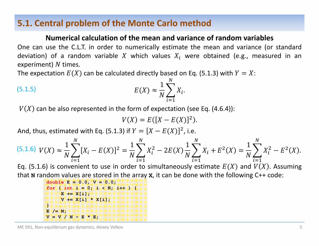
Numerical calculation of the mean and variance of random variablesOne can use the C.L.T. in order to numerically estimate the mean and variance (or standarddeviation) of a random variable which values were obtained (e.g., measured in anexperiment) times.The expectation can be calculated directly based on Eq. (5.1.3) with :

1.

can be also represented in the form of expectation (see Eq. (4.6.4)):.

And, thus, estimated with Eq. (5.1.3) if , i.e.

1 1

21 1

.

Eq. (5.1.6) is convenient to use in order to simultaneously estimate and . Assumingthat N random values are stored in the array X, it can be done with the following C++ code:

double E = 0.0, V = 0.0;for ( int i = 0; i < N; i++ ) {

E += X[i];V += X[i] * X[i];

}E /= N;V = V / N – E * E;



(5.1.5)

(5.1.6)


5.1. Central problem of the Monte Carlo method Calculation of an integral by means on sampling of random variables

Calculation of an integral based on the C.L.T. reduces to obtaining multiple independent randomvariables with the same distribution. The process of obtaining multiple independent realizationsof a random variables is referred to as sampling. The obtained vector of values

, , , … , is called the sample, and the number of variables in the sample is calledthe sample size. Special algorithm/code used to sample a random variable with a givendistribution is called the generator of this random variable.In order to find given by Eq. (5.1.1) we need to make three steps:1. Find such PDF and function , that

.

2. Develop a generator of variable with given PDF .3. Generate sample of the large size and use Eq. (5.1.4).The C.L.T. provides us with the estimate for the error of the numerically calculated integral :

~ .

There are two general ways to decrease the error of the MC estimate: To increase or todecrease . The convergence of to with increasing is slow.

(5.1.7)

(5.1.8)

Obviously, the choice of functions and in Eq. (5.1.7) is non‐unique. One can use thisfreedom and look for such and that provides minimum .Example: Use the MC method in order to calculate the integral

cos 2 sin 2 .

Let's use in the form of a standard continuous variable with uniform distribution in theinterval from 0 to 1 and PDF equal to (see slide 23 in Chapter 4)

1, 0 1;0, 0or 1.

Then , where cos 2 sin 2 .

Let's assume that can be generated with the computer function brng().C++ implementation of the code for this problem:

double Integral ( int N ) // N is the sample size{double E = 0.0, M_PI = 3.1415926;

for ( int i = 0; i < N; i++ ) {double X = brng ();E += cos ( M_PI * X / 2.0 ) * sin ( M_PI * X / 2.0 );

}return E / N;

}




5.1. Central problem of the Monte Carlo method Reduction of an integral to a form of expectation

Let's consider the general approach to the choice of and .

.

Let’s consider an arbitrary random variable with a PDF which has a non zero values in theinterval from to : 0 at . Then let’s introduce a new random variable withthe PDF

0 or

.

Here we need to dived by in order to satisfy the normalization condition for PDF, Eq. (4.6.3). Then integral can be represented in the form

, where .

If possible, must be chosen in order to reduce variance of .

(5.1.10)

(5.1.11)

(5.1.9)

Two practical requirements to the choice of : We should be able to easily sample values of the random variable with given PDF. Random variable must have as small as possible variance.If, however, large variance is not a concern in the problem under consideration and and arefinite, then one can use the uniform distribution in Eq. (5.1.11).

Monte Carlo calculation of an integral based on the uniform distributionLet's assume that and in Eq. (5.1.9) are finite, then one can always introduce the randomvariable with the uniform distribution between and with PDF (see Eq. (4.7.1))

1/0 or

Then we can re‐write the integral in the form

and the MC estimate for such takes the form

.



(5.1.12)

(5.1.13)

The estimate can be viewed as an average value of the integrand within the integration interval multiplied by the length of the

interval ( )


5.1. Central problem of the Monte Carlo method Note that Eq. (5.1.13) is similar to the equation for the rectangle quadrature rule on a meshwith equal spacing:

∆ , where∆ , 1 ∆ .

The MC estimate, Eq. (5.1.13), cannot be more computationally “effective” than the rectanglerule. The MC method, however, can be preferable if

We need to calculate multidimensional integrals (such integrals regularly appear, e.g., in thestatistical physics). When we calculate an ‐dimensional integral with nodes in everycoordinate direction, the total number of quadrature nodes is equal to .

The domain of integration of multidimensional integrals is geometrically complex.

Under such conditions, the MC estimate can be more effective, i.e. it allows one to findintegrals with smaller sample size than the number of quadrature nodes in Eq. (5.1.14).

Additionally, the MC method can be used to estimate integrals under conditions when isunknown, but random variables can be obtained as a result of MC imitation of the evolvingrandom process (system). This principle is used, in particular, in the Direct Simulation MonteCarlo method for rarefied gas flows.

(5.1.14)


5.2. Random and pseudo‐random numbers Standard approach to sampling of random variable with given distribution Random numbers Pseudo‐random numbers Basic random number generator based on Multiply With Carry (MWC) algorithm


5.2. Random and pseudo‐random numbers Standard approach to sampling of random variable with given distribution

The standard approach for sampling of random variable with given distribution is usuallybased on the transformation of random variables and includes two steps:1. First, one can develop a method (approach, algorithm, generator) for sampling of random

numbers , i.e. standard continuous random variable with uniform distribution in theinterval from 0 and 1 (See slide 23 in Chapter 4).

2. Next, one can develop an equation (method, algorithm, generator) that allows one to findby transforming random numbers, i.e. as a function of single or multiple random numbers

, , , … .

Random numbersRandom number is the standard random variable with uniform distribution is distributed inthe interval [0,1] with the PDF

1, 0 1;0, 0or 1,

0, 0;, 0 1;1, 1.

(5.2.1)


5.2. Random and pseudo‐random numbers Major properties of random numbers:1. If 0 1, then .2. Moments of random numbers

11 .

3. Mean

12 .

3. Variance

12

13

14

112 .

4. If a random number is written in decimal form, 0. …, then every individualdigit is a discrete random variable with uniform distribution, i.e. every decimal number 0,1, 2, 3, …, 9 must occurs in every with the same frequency.

(5.2.3)

0 1

1

1

(5.2.2)

(5.2.4)

(5.2.5)


5.2. Random and pseudo‐random numbers Practical implementation of true random number with digital computers is a difficult problem.Generation of true random numbers is possible by using carefully designed physical devices. Incalculations with digital computers, the true random numbers are replaces with the so‐calledpseudo‐random numbers.

Pseudo‐random numbersPseudo‐random numbers are calculated using some deterministic (not stochastic) approach,and, thus, they are not random at all. But the statistical properties of such pseudo‐randomnumbers are close to corresponding properties of true random numbers. In particular, themoments of distribution of pseudo‐random numbers are close to moments of random numbersgiven by Eq. (5.2.3). Practically, it means that large sets (samples) of pseudo‐random numbersbehave like large samples of true random numbers.Generators of pseudo‐random numbers are often called basic random number generators(BRNGs). Usually the BRNGs are implemented in the form of a deterministic equation(algorithm) that allows one to calculate new realization of a random number based on theprevious realizations , , ...

Γ , , … , .

Every time when we use the same , , … , in Eq. (5.2.6), it produces the same and,thus, is not a random variable.

(5.2.6)


5.2. Random and pseudo‐random numbers The process of calculation of pseudo‐random number with Eq. (5.2.6) can be illustrated with thefollowing sketch

In order to start calculations at 1 we need to set values of , , … , . These valuesare called the seed. One can prove that for any algorithm with finite implemented on digitalcomputers, there is only a finite non‐recurring sequence of length of pseudo‐randomnumbers. At , all numbers will be repeated with period . It is dangerous to use a BRNGin order to generate more than numbers. In this case the results can be affect by thedeterministic nature of pseudo‐random numbers.Implementations of BRNGs in computer codes usually include two functions:void SetSeed ( int Seed ): To set value of the seed. The seed is often set based on thecurrent system computer time.double brng (): To generate a new pseudo‐random numbers.

... ... ... ... ... ... ... ...

Seed

Non‐recurring sequence of length Recurring sequence


5.2. Random and pseudo‐random numbers Usually, the software packages initialize the seed with a constant value at the start of the code.That is why if SetSeed () is not applied, every individual run of the code will provide the samesequence of random numbers. It is convenient for debug of the code, since at every run we willhave the same results. For final calculations, SetSeed () should be used if simulations aresupposed to be restarted. This function is usually called only once at the beginning of theexecution of the code. Then after a restart, the simulation will be continued with differentsequences of random numbers. The typical C++ code then looks likeint main ( int argc, char **argv )

{

time_t t;

SetSeed ( unsigned ( time ( &t ) ) );

// No calls of SetSeed below

float v1 = brng ();

...

}

In MATLAB, the BRNG is implemented in the form of functions :To set seed: rng ( seed ), where seed is the nonnegative integer seed.To generate random number:rand ()

In C++, the standard library does not contain a BRNG.

The "quality" of various BRNGs is defined by a few factors including: Difference of moments of BRNG from moments given by Eq. (5.2.3). Usually, the error

increases with increasing order of moments. Difference in distributions of individual digits from uniform distributions if the random

number is represented in the form 0. … . Usually, the degree of deviation ofdistribution for from uniform increases with increasing .

Size of the period. Sensitivity of aforementioned quantities to the choice of the initial seed.Good BRNGs can be obtained even with 1 in Eq. (5.2.6), when it reduces to

Γ .In particular the practically important generator can be obtained with the simple equation

,

where denotes the fractional part of real number and 5 .Such simple methods, however, are sensitive to the initial seed, and provide good sequence ofpseudo‐random number only for specific . In addition, Eq. (5.2.8) is not convenient for realcalculations, because it requires manipulations with large integer values which do not fit to theinteger variable types in programming languages. For real calculations, some equivalent form ofEq. (5.2.8) is usually used.ME 591, Non‐equilibrium gas dynamics, Alexey Volkov 17

5.2. Random and pseudo‐random numbers

(5.2.7)

(5.2.8)

Basic random number generator based on Multiply With Carry (MWC) algorithm Simple, but effective and reliable Multiply With Carry (MWC) algorithm was proposed by GeorgeMarsaglia. It can be implemented in the form of C++ code as follows:

// Variables containing current state of the generator// Values here correspond to the default stateunsigned int m_u = 521288629, m_v = 362436069;void SetSeed ( unsigned int u, unsigned int v = unsigned (362436069 ) ){

m_u = u;m_v = v;

}unsigned int IntUniform ( unsigned int& u, unsigned int& v ){

v = 36969*(v & 65535) + (v >> 16);u = 18000*(u & 65535) + (u >> 16);return (v << 16) + u;

};double brng(){unsigned int z = IntUniform ( m_u, m_v );

return z*2.328306435996595e-10;}

This BRNG in a slightly general form is implemented in the file BRNG.cxx posted on theblackboard.ME 591, Non‐equilibrium gas dynamics, Alexey Volkov 18


This code initially generates a pseudo‐random integer distributed uniformly from 0 to 232‐1, so the period for this generator cannot be larger than 232.

Currently, in many software packages, the BRNG implementation is based on theMT (MersenneTwister) algorithm suggested inM. Matsumoto and T. Nishimura, "Mersenne Twister: A 623‐Dimensionally EquidistributedUniform Pseudo‐Random Number Generator", ACM Transactions on Modeling and ComputerSimulation, Vol. 8, No. 1, January 1998, p. 3‐30.There are a lot of free C++ implementations of this algorithm available in the internet, see, e.g.,http://pages.cs.wisc.edu/~stjones/proj/randistrs.chttps://github.com/frt/mtwist/blob/master/randistrs.c




5.3. Sampling of discrete random variables Standard method of sampling of discrete random variables Uniform distribution Poisson distribution


5.3. Sampling of discrete random variablesStandard method of sampling of discrete random variables

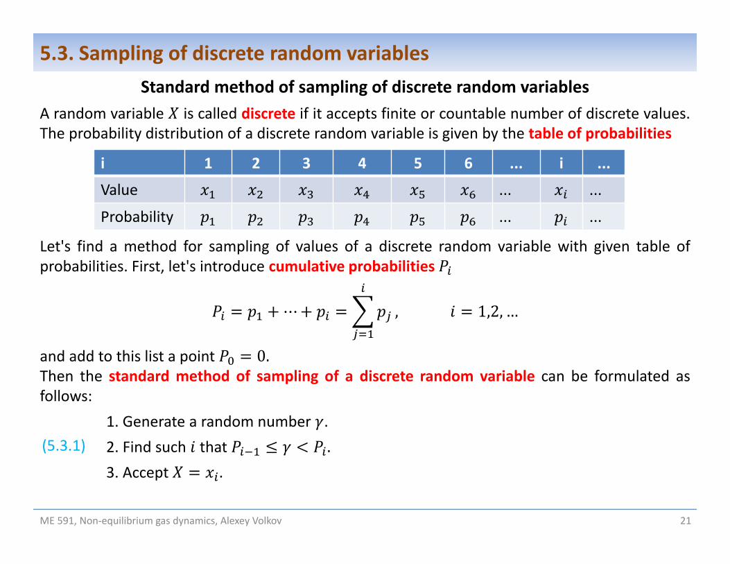
A random variable is called discrete if it accepts finite or countable number of discrete values.The probability distribution of a discrete random variable is given by the table of probabilities

Let's find a method for sampling of values of a discrete random variable with given table ofprobabilities. First, let's introduce cumulative probabilities

⋯ , 1,2, …

and add to this list a point 0.Then the standard method of sampling of a discrete random variable can be formulated asfollows:

1. Generate a random number .2. Find such that .3. Accept .

i 1 2 3 4 5 6 ... i ...

Value ... ...

Probability ... ...

(5.3.1)

In order to prove this algorithm of the standard method, let's simply note that.

The standard method can be implemented in the following C++ code:// Pcum is an array of cumulative probabilities// Individual values are indexed by the index i = 0,...,N-1

double frand_discrete_std ( int N, double *X, double *Pcum ){int i = 0;double Gamma = brng ();

while ( Gamma > Pcum[i] ) i++;return X[i];

}


5.3. Sampling of discrete random variables

0

1

D.F. of with 4 possible values

For specific distributions, other methods exist. We consider only two examples.

Uniform distributionLet's consider a discrete random variable which takes integer values from 0 to 1 with theuniform distribution, i.e. with equal probabilities, i.e. with the probability table

1, 1.

Then such a random variable can be sample with equation

,

where means the integer part of number .

C++ implementation of this method:

int irand_uniform ( int N ){

return int ( N * brng () );}



(5.3.2)

(5.3.3)

Poisson distributionLet's consider a discrete random variable which takes integer values from 0 to ∞ with thePoisson distribution, i.e. with probabilities (see Slides 16 and 17 in Chapter 4)

! ,

where parameter .It can be proved that such a random variable can be sampled with equation

min 1,2, … 1.

C++ implementation of this method:int irand_Poisson ( double E ){double expE = exp ( - E ); double prod = 1.0;int i = 0;

do {i++;prod *= brng ();

} while ( prod >= expE );return i - 1;

}



(5.3.4)

(5.3.5)


5.4. Sampling of continuous random variables Standard method of sampling of continuous random variables Uniform distribution in a finite interval Rayleigh distribution Sampling of random vectors with independent coordinates Gaussian distribution Sampling of random velocities of gas molecules with the Maxwell‐Boltzmann

distribution Acceptance and rejection method Calculation of two‐dimensional integrals with the acceptance and rejection method Acceptance and rejection method for sampling of continuous random variables Random vectors with uniform distribution of directions (Isotropic vectors)


5.4. Sampling of continuous random variablesStandard method of sampling of continuous random variables

Let' assume that we want to sample a continuous random variable with a given distributionfunction that satisfied the condition

/ 0 for all where 0 1.

It means, in particular, that there is a function inverse to , i.e., .

Let's show then that the random variable can be sampled with the equation,

where is the random number. In order to prove it, let’s show that variable defined by Eq.(5.4.2) has the distribution function :

.Equation (5.4.2) defines the standard method of sampling of continuous random variables. Itcan be applied only if condition given by Eq. (5.4.1) is met.

1

0

1

0

0

(5.4.1)

(5.4.2)


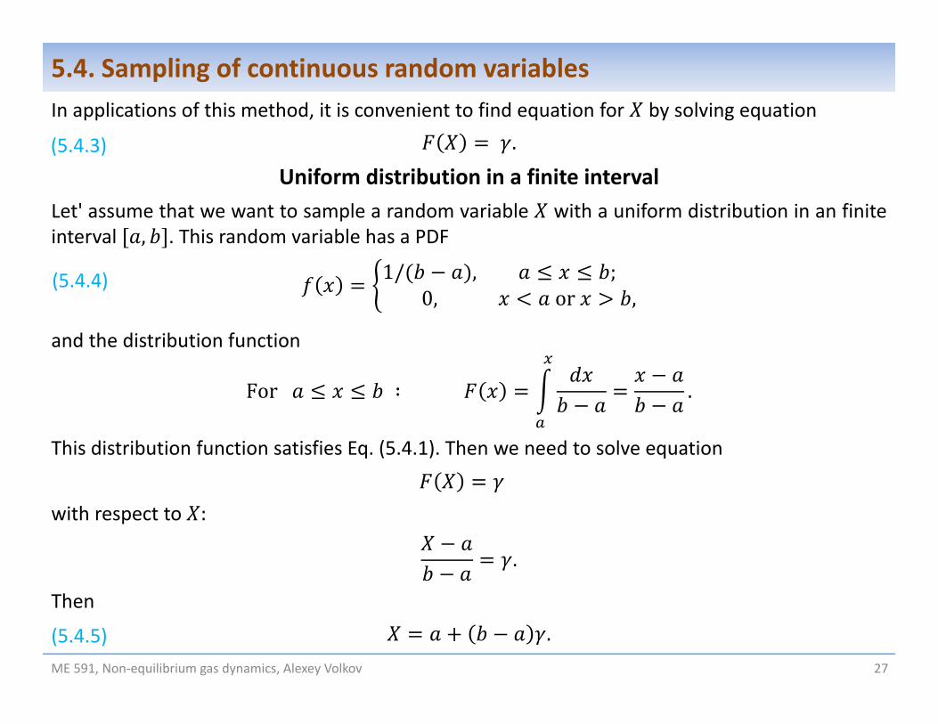
5.4. Sampling of continuous random variablesIn applications of this method, it is convenient to find equation for by solving equation

.Uniform distribution in a finite interval

Let' assume that we want to sample a random variable with a uniform distribution in an finiteinterval , . This random variable has a PDF

1/ , ;0, or ,

and the distribution function

For ∶ .

This distribution function satisfies Eq. (5.4.1). Then we need to solve equation

with respect to :

.

Then.

(5.4.4)

(5.4.5)

(5.4.3)


5.4. Sampling of continuous random variablesRayleigh distribution

We say that a non‐negative continuous variable has the Rayleigh distribution with parameterif its PDF at 0 is equal to

exp 2 .

Then the distribution function is equal to

exp 2 1 exp 2 .

This satisfies Eq. (5.4.1) and then in order to find we need to solve the equation

or1 exp 2 .

Then

2 log 1 .

But and 1 have the same distribution, so that

2 log .

(5.4.6)

(5.4.7)


5.4. Sampling of continuous random variablesSampling of random vectors with independent coordinates

Let's consider a 2D random vector , where individual coordinate and are anindependent continuous random variables. According to the definition given by Eq. (4.8.8) itmeans that

, .

The individual independent components of random vectors can be sampled independently.

Example 1: Let's assume that we want to sample a point withindependent coordinates that is uniformly distributed in arectangle , , .

, , .

1,

1.

Then random coordinates of the point are

,.

(5.4.8)

(5.4.9)


5.4. Sampling of continuous random variablesExample 2: Let's assume that we want to sample a random point uniformly distributed in a circleof radius with center in the point , .In order to solve the problem, we can introduce the random variables and corresponding topolar coordinates on the plane , .

cos , sin , .Since the point has uniform distribution, then

, , , cos , sin , , ,

, ,2 1

2 ,

where2

, 12

Thus, according to Eq. (5.4.8), random variables andare independent. The distribution functions of thesevariables are equal to

, 2 .

,

(5.4.9)

Then equations for sampling and can be found fromby solving equations

, 2 ,

which results to, 2 .

The equations for and can be found from Eq. (5.4.9):

cos , sin .


5.4. Sampling of continuous random variables

C++ implementation of this algorithm (see file Point2DUniformCircleRNG.cxx ):void v2rand_circle ( double &X, double &Y, double a, double b, double R )

{

double M_PI = 3.1415926;

double R1 = R * sqrt ( brng () );

double E1 = 2.0 * M_PI * brng ();

X = a + R1 * cos ( E1 );

Y = b + R1 * sin ( E1 );

}

,

(5.4.10)

(5.4.11)

Gaussian distributionAn explicit equation for modelling of the Gaussian distribution cannot be obtained based on thestandard method, because there is no explicit equation for . In order to find an equation forsampling a Gaussian random variable let's first consider a vector of two independent Gaussianvariables , with zero mean, variance equal to 1, and PDFs equal to

12

/ ,12

/ .

Then

, ,12

/ .

Now let's introduce random polar coordinates and on the plane , : Thencos , sin , , , , .

, , 2/ , / ,

12 .

Thus, and are independent random variables. has a Rayleigh distribution with parameter1 and is distributed uniformly between 0 and 2 . Then

2 log , 2 , cos , sin .

These equations allow one to obtain two independent samples of variable simultaneously.One can use both or only one of them as needed.ME 591, Non‐equilibrium gas dynamics, Alexey Volkov 32


(5.4.12)


5.4. Sampling of continuous random variablesA Gaussian random variable with mean and standard deviation can be obtained fromrandom variable , which has a Gaussian distribution with mean 0 and standard deviation 1 asfollows (see slides 25 and 28 in Chapter 4):

.

Eqs. (5.4.12) and (5.4.13) give the standard method of sampling of Gaussian random variables.

C++ implementation of this method (see file GaussianRNG.cxx):double frand_Gaussian ( double E, double V ) // Here V is the variance

{

double M_PI = 3.1415926;

return E + sqrt ( - 2.0 * V * log ( brng () ) ) * cos ( 2.0 * M_PI * brng () );

}

Sampling of random velocities of gas molecules with the Maxwell‐Boltzmann distribution

Let’s assume that we want to generate a random velocity vector of a molecule in the gas inthe equilibrium state, where the velocity distribution function is equal to the Maxwell‐Boltzmann distribution function given by Eq. (3.6.9):

2 / exp 2 .

(5.4.13)

In order to develop a method for sampling of random components of the velocity vector, , , the Maxwell‐Boltzmann distribution function must be first turned into the form of a

joint PDF. Any PDF must satisfy the normalization condition, Equation (4.6.2). It means that thePDF of is equal to

, , , ,1

2 / exp 2 ,

12 / exp 2 .

These equations show that Velocity components , , are independent random variables;

PDF of an individual velocity component, e.g., is the Gaussian PDF with expectationand standard deviation .

Sampling of velocity components from the Maxwell‐Boltzmann distribution reduces to samplingof Gaussian random variables and can be performed with the following C++ code:void vrand_MB ( double *v, double m, double *u, double T ){double RT = BOLTZMANN_CONSTANT * T / m;

v[0] = frand_Gaussian ( u[0], RT );v[1] = frand_Gaussian ( u[1], RT );v[2] = frand_Gaussian ( u[2], RT );

}



(5.4.14)


5.4. Sampling of continuous random variablesAcceptance and rejection method

Let's consider a point with random coordinates , that is uniformly distributed in a finitedomain of complex shape on the plane , . The uniformity of distribution means that

point inside ,

where is the area of . If is not a rectangle with facesparallel to axes and , then random variables andare not independent (see example in slide 32 of Chapter 4).But they can be sampled with the acceptance and rejectionmethod as follows1. Let's find such rectangle , , that includes thefull domain .2. Generate a random point , with uniform distributioninside the rectangle , , :

, .3. Check the position of the point , with respect to .If the point inside , then , is accepted as the nextrealization of coordinates of the random point. If not, thepoint is rejected and algorithm returns to step 2. Randompoints must be generated in a loop until a point inside isfound.

Domain of area

(5.4.15)

(5.4.14)


5.4. Sampling of continuous random variablesCalculation of two‐dimensional integrals with the acceptance and rejection method

,

First, let's represent this integral in the form of an expectation:

, , , , , ,1.

Here is the area of and , , is the joint PDF of , with uniform distribution in .Then the integral can be estimated as

, ,

where , are coordinates of a random point distributed uniformly in the domain . Theserandom coordinates can be generated with the acceptance and rejection method. The area ofthe domain D can be also calculated with the acceptance and rejection method as follows:

Point , withcoordinatesinEq. 5.4.15 isinside ,

Numberofacceptedpoints

Totalnumberofpoints generatedwithEq. 5.4.15 .

(5.4.16)

(5.4.17)

The estimate can be viewed as an average value of the integrand within the domain multiplied by the area of the

domain: Compare with Eq. (5.1.13)


5.4. Sampling of continuous random variablesThen Eq. (5.4.16) can be re‐written as

, .

In order to implement this method for practical calculations we only need to develop ofcomputer function that checks whether a point with given coordinates , is inside or not.Example: Calculate the integral

sin ,

(5.4.18)

where is the superposition of twopartially overlapping rectangles asshown in the sketch by green. Inthis case point , belongs to ifand only if it belongs at least to oneof rectangles.


5.4. Sampling of continuous random variablesThen the MC estimate of can be obtained at arbitrary , , , and 1,2 with thefollowing C++ code:

int N = 100000; // Desired size of the sample of accepted points

double a[2], b[2], c[2], d[2]; // Coordinates of the rectangle edges

bool IsPointInsideD ( double X, double Y ) /////////////////////////////////////////////////{

for ( int i = 0; i < 2; i++ )if ( X >= a[i] && X <= b[i] && Y >= c[i] && Y <= d[i] ) return true;

return false;}

double Integral() // This function returns value of I_N ////////////////////////////////////{double x_min = ( a[0] < a[1] ) ? a[0] : a[1];double x_max = ( b[0] > b[1] ) ? b[0] : b[1];double y_min = ( c[0] < c[1] ) ? c[0] : c[1];double y_max = ( d[0] > d[1] ) ? d[0] : d[1];int Ntot = 0; // Total number of generated points in the acceptance and rejection methoddouble IN = 0.0;

for ( int i = 0; i < N; i++ ) {double X, Y;do {

X = x_min + ( x_max - x_min ) * brng ();Y = y_min + ( y_max - y_min ) * brng ();Ntot++;

} while ( !IsPointInsideD ( X, Y ) );IN += ( X + Y ) * ( X + Y ) * sin ( exp ( - X ) );

}return (( x_max - x_min ) * ( y_max - y_min ) * IN / Ntot ); // Eq. (5.4.18)

}


5.4. Sampling of continuous random variablesAcceptance and rejection method for sampling of continuous random variables

Let's consider a continuous random variable with given PDF , which satisfies twoconditions: 0 in a finite interval [a,b] and 0 outside , . Values of are finite inside , , i.e. such constant exists that

forall .

One can prove that if we introduce a random vector, which corresponds to a point distributed

uniformly in the domain (greed area in thesketch) bounded by the axis , plot of the function

, and vertical lines and , thenrandom coordinate of this point has PDF .The proof of this statement can be performedbased on the notions of conditional probabilitiesand conditional PDFs.Then the sampling of random variable reduces tothe sampling of a point in the domain with theacceptance and rejection method.

Domain


5.4. Sampling of continuous random variablesIf one preliminary found , then the algorithm of the acceptance and rejection method forsampling of can be formulated as follows:1. Generate a random point with coordinates ,

, .2. Check the condition

.

If this condition is satisfied, then is accepted as the value of random variable with PDF ,otherwise the algorithm returns to step 1 and new random point is generated .

C++ implementation of the acceptance and rejection method (see file ARMRNG.cxx):

double frand_arm ( double a, double b, double c, double (*pdf) ( double X ) )

{

double X, Y;

do {

X = a + ( b - a ) * brng ();

Y = c * brng ();

} while ( Y > pdf ( X ) ); // Condition opposite to Eq. (5.4.19)

return X;

}

(5.4.19)


5.4. Sampling of continuous random variablesRandom vectors with uniform distribution of directions (Isotropic vectors)

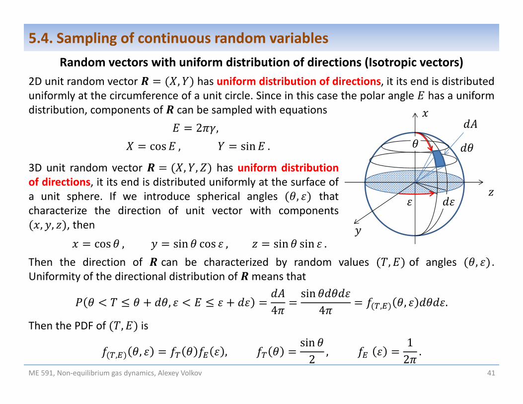
2D unit random vector , has uniform distribution of directions, it its end is distributeduniformly at the circumference of a unit circle. Since in this case the polar angle has a uniformdistribution, components of can be sampled with equations

2 ,cos , sin .

cos , sin cos , sin sin .Then the direction of can be characterized by random values , of angles , .Uniformity of the directional distribution of means that

, 4sin

4 , , .

Then the PDF of , is

, , ,sin2 ,

12 .

3D unit random vector , , has uniform distributionof directions, it its end is distributed uniformly at the surface ofa unit sphere. If we introduce spherical angles , thatcharacterize the direction of unit vector with components, , , then

Thus, and are independent random variables with distribution functions:

1cos2 , 2 .

Thus, cos and have uniform distribution and random components of , , can besampled as follows:

cos 1 2 , 2 ,

sin 1 cos ,cos , sin co , sin sin .

C++ implementation of this algorithm (see file IsotropicVectorRNG.cxx):void v3rand_isotropic ( double *R )

{

double M_PI = 3.1415926;

double cosT = 1.0 - 2.0 * brng ();

double sinT = sqrt ( 1.0 - cosT * cosT );

double E = 2.0 * M_PI * brng ();

R[0] = cosT;

R[1] = sinT * cos ( E );

R[2] = sinT * sin ( E );

}



Random vectors with uniformdistribution of directions aresometimes called isotropic.

(5.4.19)


5.5. Sampling of random eventsSampling of random events

Let's assume that in the course of a simulation some random event (change of state of asystem under consideration) occurs with given probability . How can we sample/draw suchrandom event during the simulations process?Examples:1. We have two molecules and which collide each other during time ∆ with given probability

1. How can we decide whether collision happens or not during ∆ ?

2. We simulate an excited atom that can emit a photon during time ∆ with known probability1. How can we decide whether the random emission occurs or not?

Sampling of random evens during Monte Carlo simulations is based on the major property ofrandom numbers given by Eq. (5.2.2):

If 0 1 then .We can apply this property to :

,i.e. probabilities of random events and are identical. It means that every time whenwe need to decide whether the random even occurs or not, we can use the following approach:1. Sample and check whether or not.2. If it is true, then the random even occurs, otherwise it does not occur.

(5.5.1)

Documents

Chapter 5 Monte Carlo method - volkov.eng.ua.edu