THE MODULI SPACE OF CURVES AND GROMOV-WITTENTHEORY

RAVI VAKIL

ABSTRACT. The goal of this article is to motivate and describe how Gromov-Witten the-ory can and has provided tools to understand the moduli space of curves. For example,ideas and methods from Gromov-Witten theory have led to both conjectures and theoremsshowing that the tautological part of the cohomology ring has a remarkable and profoundstructure. As an illustration, we describe a new approach to Faber’s intersection numberconjecture via branched covers of the projective line (work with I.P. Goulden and D.M.Jackson, based on work with T. Graber). En route we review the work of a large number ofmathematicians.

CONTENTS

1. Introduction 1

2. The moduli space of curves 3

3. Tautological cohomology classes on moduli spaces of curves, and theirstructure 12

4. A blunt tool: Theorem ? and consequences 31

5. Stable relative maps to P1 and relative virtual localization 35

6. Applications of relative virtual localization 44

7. Towards Faber’s intersection number conjecture ?? via relative virtuallocalization 47

8. Conclusion 51

References 52

1. INTRODUCTION

These notes are intended to explain how Gromov-Witten theory has been useful inunderstanding the moduli space of complex curves. We will focus on the moduli spaceof smooth curves and how much of the recent progress in understanding it has comethrough “enumerative” invariants in Gromov-Witten theory, something which we take

Date: Sunday, February 19, 2006.Partially supported by NSF CAREER/PECASE Grant DMS–0228011, and an Alfred P. Sloan Research

Fellowship.2000 Mathematics Subject Classification: Primary 14H10, 14H81, 14N35, Secondary 14N10, 53D45,

14H15.

1

for granted these days, but should really be seen as surprising. There is one sense in whichit should not be surprising — in many circumstances, modern arguments can be looselyinterpreted as the fact that we can understand curves in general by studying branchedcovers of the complex projective line, as all curves can be so expressed. We will see thistheme throughout the notes, from a Riemann-style parameter count in §2.2 to the tool ofrelative virtual localization in Gromov Witten theory in §5.

These notes culminate in an approach to Faber’s intersection number conjecture usingrelative Gromov-Witten theory (joint work with Goulden and Jackson [GJV3]). One mo-tivation for this article is to convince the reader that our approach is natural and straight-forward.

We first introduce the moduli space of curves, both the moduli space of smooth curves,and the Deligne-Mumford compactification, which we will see is something forced uponus by nature, not arbitrarily imposed by man. We will then define certain geometricallynatural cohomology classes on the moduli space of smooth curves (the tautological sub-ring of the cohomology ring), and discuss Faber’s foundational conjectures on this sub-ring. We will then extend these notions to the moduli space of stable curves, and discussFaber-type conjectures in this context. A key example is Witten’s conjecture, which re-ally preceded (and motivated) Faber’s conjectures, and opened the floodgates to the lastdecade’s flurry of developments. We will then discuss other relations in the tautologicalring (both known and conjectural). We will describe Theorem ? (Theorem 4.1), a blunttool for proving many statements, and Y.-P. Lee’s Invariance conjecture, which may giveall relations in the tautological ring. In order to discuss the proof of Theorem ?, we willbe finally drawn into Gromov-Witten theory, and we will quickly review the necessarybackground. In particular, we will need the notion of “relative Gromov-Witten theory”,including Jun Li’s degeneration formula [Li1, Li2] and the relative virtual localizationformula [GrV3]. Finally, we will use these ideas to tackle Faber’s intersection numberconjecture.

Because the audience has a diverse background, this article is intended to be read atmany different levels, with as much rigor as the reader is able to bring to it. Unless thereader has a solid knowledge of the foundations of algebraic geometry, which is mostlikely not the case, he or she will have to be willing to take a few notions on faith, and toask a local expert a few questions.

We will cover a lot of ground, but hopefully this article will include enough backgroundthat the reader can make explicit computations to see that he or she can actively manip-ulate the ideas involved. You are strongly encouraged to try these ideas out via the exer-cises. They are of varying difficulty, and the amount of rigor required for their solutionshould depend on your background.

Here are some suggestions for further reading. For a gentle and quick introduction tothe moduli space of curves and its tautological ring, see [V2]. For a pleasant and very de-tailed discussion of moduli of curves, see Harris and Morrison’s foundational book [HM].An on-line resource discussing curves and links to topology (including a glossary of im-portant terms) is available at [GiaM]. For more on curves, Gromov-Witten theory, andlocalization, see [HKKPTVVZ, Chapter 22–27], which is intended for both physicists and

2

FIGURE 1. A complex curve, and its real “cartoon”

mathematicians. Cox and Katz’ wonderful book [CK] gives an excellent mathematicalapproach to mirror symmetry. There is as of yet no ideal book introducing (Deligne-Mumford) stacks, but Fantechi’s [Fan] and Edidin’s [E] both give an excellent idea of howto think about them and work with them, and the appendix to Vistoli’s paper [Vi] laysout the foundations directly, elegantly, and quickly, although this is necessarily a moreserious read.

Acknowledgments. I am grateful to the organizers of the June 2005 conference in Ce-traro, Italy on “Enumerative invariants in algebraic geometry and string theory” (KaiBehrend, Barbara Fantechi, and Marco Manetti), to Fondazione C.I.M.E. (Centro Inter-nazionale Matematico Estivo), and to the Hotel San Michele. I learned this material frommy co-authors Graber, Goulden, and Jackson, and from the other experts in the field, in-cluding Carel Faber, Rahul Pandharipande, Y.-P. Lee, . . . , whose names are mentionedthroughout this article. I thank Carel Faber, Soren Galatius, Tom Graber, Y.-P. Lee andRahul Pandharipande for improving the manuscript.

2. THE MODULI SPACE OF CURVES

We begin with some conventions and terminology. We will work over C, although thesequestions remain interesting over arbitrary fields. We will work algebraically, and henceonly briefly mention other important approaches to the subjects, such as the constructionof the moduli space of curves as a quotient of Teichmuller space.

By smooth curve, we mean a compact (also known as proper or complete), smooth (alsoknown as nonsingular) complex curve, i.e. a Riemann surface, see Figure 1. Our curveswill be connected unless we especially describe them as “possibly disconnected”. In gen-eral our dimensions will be algebraic or complex, which is why we refer to a Riemannsurface as a curve — they have algebraic/complex dimension 1. Algebraic geometerstend to draw “half-dimensional” cartoons of curves (see also Figure 1).

The reader likely needs no motivation to be interested in Riemann surfaces. A naturalquestion when you first hear of such objects is: what are the Riemann surfaces? Howmany of them are there? In other words, this question asks for a classification of curves.

2.1. Genus. A first invariant is the genus of the smooth curve, which can be interpreted inthree ways: (i) the number of holes (topological genus; for example, the genus of the curvein Figure 1 is 3), (ii) dimension of space of space of differentials (= h0(C,ΩC), geometric

3

genus), and (iii) the first cohomology group of the sheaf of algebraic functions (h1(C,OC),arithmetic genus). These three notions are the same. Notions (ii) and (iii) are related bySerre duality

(1) H0(C,F) ×H1(C,K⊗ F∗) → H1(C,K) ∼= C

where K is the canonical line bundle, which for smooth curves is the sheaf of differentialsΩC. Here F can be any finite rank vector bundle;Hi refers to sheaf cohomology. Serre du-ality implies that h0(C,F) = h1(C,K⊗F∗), hence (taking F = K). h0(C,ΩC) = h1(C,OC).(We will use these important facts in the future!)

As we are working purely algebraically, we will not discuss why (i) is the same as (ii)and (iii).

2.2. There is a (3g− 3)-dimensional family of genus g curves.

Remarkably, it was already known to Riemann [R, p. 134] that there is a “3g − 3-dimensional family of genus g curves”. You will notice that this can’t possibly be rightif g = 0, and you may know that this isn’t right if g = 1, as you may have heard thatelliptic curves are parametrized by the j-line, which is one-dimensional. So we will takeg > 1, although there is a way to extend to g = 0 and g = 1 by making general enoughdefinitions. (Thus there is a “(−3)-dimensional moduli space” of genus 0 curves, if youdefine moduli space appropriately — in this case as an Artin stack. But that is anotherstory.)

Let us now convince ourselves (informally) that there is a (3g− 3)-dimensional familyof genus g curves. This will give me a chance to introduce some useful facts that we willuse later. I will use the same notation for vector bundles and their sheaves of sections.The sheaf of sections of a line bundle is called an invertible sheaf.

We will use five ingredients.

(1) Serre duality (1). This is a hard fact.

(2) The Riemann-Roch formula. If F is any coherent sheaf (for example, a finite rank vectorbundle) then

h0(C,F) − h1(C,F) = degF − g+ 1.

This is an easy fact, although I will not explain why it is true.

(3) Line bundles of negative degree have no non-zero sections: if L is a line bundle of

negative degree, then h0(C,L) = 0 . Here is why: the degree of a line bundle L can be

defined as follows. Let s be any non-zero meromorphic section of L. Then the degree ofL is the number of zeros of s minus the number of poles of s. Thus if L has an honestnon-zero section (with no poles), then the degree of s is at least 0.

Exercise. If L is a degree 0 line bundle with a non-zero section s, show that L is isomorphicto the trivial bundle (the sheaf of functions) O.

4

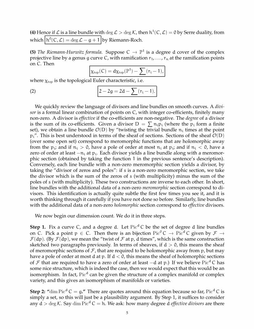
(4) Hence if L is a line bundle with degL > degK, then h1(C,L) = 0 by Serre duality, from

which h0(C,L) = degL − g+ 1 by Riemann-Roch.

(5) The Riemann-Hurwitz formula. Suppose C → P1 is a degree d cover of the complexprojective line by a genus g curve C, with ramification r1, . . . , rn at the ramification pointson C. Then

χtop(C) = dχtop(P1) −

∑(ri − 1),

where χtop is the topological Euler characteristic, i.e.

(2) 2− 2g = 2d−∑

(ri − 1).

We quickly review the language of divisors and line bundles on smooth curves. A divi-sor is a formal linear combination of points on C, with integer co-efficients, finitely manynon-zero. A divisor is effective if the co-efficients are non-negative. The degree of a divisoris the sum of its co-efficients. Given a divisor D =

∑nipi (where the pi form a finite

set), we obtain a line bundle O(D) by “twisting the trivial bundle ni times at the pointpi”. This is best understood in terms of the sheaf of sections. Sections of the sheaf O(D)

(over some open set) correspond to meromorphic functions that are holomorphic awayfrom the pi; and if ni > 0, have a pole of order at most ni at pi; and if ni < 0, have azero of order at least −ni at pi. Each divisor yields a line bundle along with a meromor-phic section (obtained by taking the function 1 in the previous sentence’s description).Conversely, each line bundle with a non-zero meromorphic section yields a divisor, bytaking the “divisor of zeros and poles”: if s is a non-zero meromorphic section, we takethe divisor which is the sum of the zeros of s (with multiplicity) minus the sum of thepoles of s (with multiplicity). These two constructions are inverse to each other. In short,line bundles with the additional data of a non-zero meromorphic section correspond to di-visors. This identification is actually quite subtle the first few times you see it, and it isworth thinking through it carefully if you have not done so before. Similarly, line bundleswith the additional data of a non-zero holomorphic section correspond to effective divisors.

We now begin our dimension count. We do it in three steps.

Step 1. Fix a curve C, and a degree d. Let PicdC be the set of degree d line bundleson C. Pick a point p ∈ C. Then there is an bijection Pic0C → PicdC given by F →F(dp). (By F(dp), we mean the “twist of F at p, d times”, which is the same constructionsketched two paragraphs previously. In terms of sheaves, if d > 0, this means the sheafof meromorphic sections of F , that are required to be holomorphic away from p, but mayhave a pole of order at most d at p. If d < 0, this means the sheaf of holomorphic sectionsof F that are required to have a zero of order at least −d at p.) If we believe PicdC hassome nice structure, which is indeed the case, then we would expect that this would be anisomorphism. In fact, Picd can be given the structure of a complex manifold or complexvariety, and this gives an isomorphism of manifolds or varieties.

Step 2: “dim PicdC = g.” There are quotes around this equation because so far, PicdC issimply a set, so this will just be a plausibility argument. By Step 1, it suffices to considerany d > degK. Say dim PicdC = h. We ask: how many degree d effective divisors are there

5

(i.e. what is the dimension of this family)? The answer is clearly d, and Cd surjects ontothis set (and is usually d!-to-1).

But we can count effective divisors in a different way. There is an h-dimensional familyof line bundles by hypothesis, and each one of these has a (d− g+ 1)-dimensional familyof non-zero sections, each of which gives a divisor of zeros. But two sections yield thesame divisor if one is a multiple of the other. Hence we get: h+(d−g+1)−1 = h+d−g.

Thus d = h+ d − g, from which h = g as desired.

Note that we get a bit more: if we believe that Picd has an algebraic structure, we havea fibration (Cd)/Sd → Picd, where the fibers are isomorphic to Pd−g. In particular, Picd

is reduced (I won’t define this!), and irreducible. (In fact, as many of you know, it isisomorphic to the dimension g abelian variety Pic0C.)

Step 3. Say Mg has dimension p. By fact (4) above, if d 0, and D is a divisor of degreed, then h0(C,O(D)) = d − g + 1. If we take two general sections s, t of the line bundleO(D), we get a map to P1 (given by p → [s(p); t(p)] — note that this is well-defined), andthis map is degree d (the preimage of [0; 1] is precisely div s, which has d points countedwith multiplicity). Conversely, any degree d cover f : C → P1 arises from two linearlyindependent sections of a degree d line bundle. (To get the divisor associated to one ofthem, consider f−1([0; 1]), where points are counted with multiplicities; to get the divisorassociated to the other, consider f−1([1; 0]).) Note that (s, t) gives the same map to P1 as(s ′, t ′) if and only (s, t) is a scalar multiple of (s ′, t ′). Hence the number of maps to P1

arising from a fixed curve C and a fixed line bundle L correspond to the choices of twosections (2(d − g + 1) by fact (4)), minus 1 to forget the scalar multiple, for a total of2d − 2g + 1. If we let the the line bundle vary, the number of maps from a fixed curveis 2d − 2g + 1 + dim Picd(C) = 2d − g + 1. If we let the curve also vary, we see that the

number of degree d genus g covers of P1 is p+ 2d− g+ 1 .

But we can also count this number using the Riemann-Hurwitz formula (2). By that for-mula, there will be a total of 2g+ 2d− 2 branch points (including multiplicity). Given thebranch points (again, with multiplicity), there is a finite amount of possible monodromydata around the branch points. The Riemann Existence Theorem tells us that given anysuch monodromy data, we can uniquely reconstruct the cover, so we have

p+ 2d − g+ 1 = 2g+ 2d− 2,

from which p = 3g− 3 .

Thus there is a 3g−3-dimensional family of genus g curves! (By showing that the spaceof branched covers is reduced and irreducible, we could again “show” that the modulispace is reduced and irreducible.)

2.3. The moduli space of smooth curves.

It is time to actually define the moduli space of genus g smooth curves, denoted Mg,or at least to come close to it. By “moduli space of curves” we mean a “parameter space

6

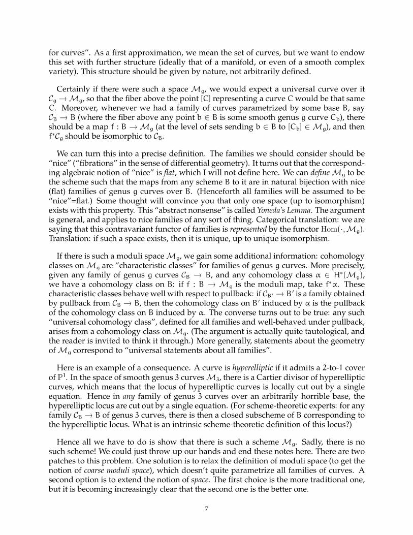
for curves”. As a first approximation, we mean the set of curves, but we want to endowthis set with further structure (ideally that of a manifold, or even of a smooth complexvariety). This structure should be given by nature, not arbitrarily defined.

Certainly if there were such a space Mg, we would expect a universal curve over itCg → Mg, so that the fiber above the point [C] representing a curve Cwould be that sameC. Moreover, whenever we had a family of curves parametrized by some base B, sayCB → B (where the fiber above any point b ∈ B is some smooth genus g curve Cb), thereshould be a map f : B → Mg (at the level of sets sending b ∈ B to [Cb] ∈ Mg), and thenf∗Cg should be isomorphic to CB.

We can turn this into a precise definition. The families we should consider should be“nice” (“fibrations” in the sense of differential geometry). It turns out that the correspond-ing algebraic notion of “nice” is flat, which I will not define here. We can define Mg to bethe scheme such that the maps from any scheme B to it are in natural bijection with nice(flat) families of genus g curves over B. (Henceforth all families will be assumed to be“nice”=flat.) Some thought will convince you that only one space (up to isomorphism)exists with this property. This “abstract nonsense” is called Yoneda’s Lemma. The argumentis general, and applies to nice families of any sort of thing. Categorical translation: we aresaying that this contravariant functor of families is represented by the functor Hom(·,Mg).Translation: if such a space exists, then it is unique, up to unique isomorphism.

If there is such a moduli space Mg, we gain some additional information: cohomologyclasses on Mg are “characteristic classes” for families of genus g curves. More precisely,given any family of genus g curves CB → B, and any cohomology class α ∈ H∗(Mg),we have a cohomology class on B: if f : B → Mg is the moduli map, take f∗α. Thesecharacteristic classes behave well with respect to pullback: if CB′ → B ′ is a family obtainedby pullback from CB → B, then the cohomology class on B ′ induced by α is the pullbackof the cohomology class on B induced by α. The converse turns out to be true: any such“universal cohomology class”, defined for all families and well-behaved under pullback,arises from a cohomology class on Mg. (The argument is actually quite tautological, andthe reader is invited to think it through.) More generally, statements about the geometryof Mg correspond to “universal statements about all families”.

Here is an example of a consequence. A curve is hyperelliptic if it admits a 2-to-1 coverof P1. In the space of smooth genus 3 curves M3, there is a Cartier divisor of hyperellipticcurves, which means that the locus of hyperelliptic curves is locally cut out by a singleequation. Hence in any family of genus 3 curves over an arbitrarily horrible base, thehyperelliptic locus are cut out by a single equation. (For scheme-theoretic experts: for anyfamily CB → B of genus 3 curves, there is then a closed subscheme of B corresponding tothe hyperelliptic locus. What is an intrinsic scheme-theoretic definition of this locus?)

Hence all we have to do is show that there is such a scheme Mg. Sadly, there is nosuch scheme! We could just throw up our hands and end these notes here. There are twopatches to this problem. One solution is to relax the definition of moduli space (to get thenotion of coarse moduli space), which doesn’t quite parametrize all families of curves. Asecond option is to extend the notion of space. The first choice is the more traditional one,but it is becoming increasingly clear that the second one is the better one.

7

This leads us to the notion of a stack, or in this case, the especially nice stack known asa Deligne-Mumford stack. This is an extension of the idea of an idea of a scheme. Defininga Deligne-Mumford stack correctly takes some time, and is rather tiring and uninspiring,but dealing with Deligne-Mumford stacks on a day-to-day basis is not so bad — you justpretend it is a scheme. One might compare it to driving a car without knowing how theengine works, but really it is more like driving a car while having only the vaguest ideaof what a car is.

Thus I will content myself with giving you a few cautions about where your informalnotion of Deligne-Mumford stack should differ with your notion of scheme. (I feel lessguilty about this knowing that many analytic readers will be similarly uncomfortablewith the notion of a scheme.) The main issue is that when considering cohomology rings(or the algebraic analog, Chow rings), we will take Q-co-efficients in order to avoid subtletechnical issues. The foundations of intersection theory for Deligne-Mumford stacks werelaid by Vistoli in [Vi] (However, thanks to work of Andrew Kresch [Kr], it is possible totake integral co-efficients using the Chow ring. Then we have to accept the fact thatcohomology groups can be non-zero even in degree higher than the dimension of thespace. This is actually something that for various reasons we want to be true, but such adiscussion is not appropriate in these notes.)

A smooth (or nonsingular) Deligne-Mumford stack (over C) is essentially the samething as a complex orbifold. The main caution about saying that they are the same thingis that there are actually three different definitions of orbifold in use, and many users areconvinced that their version is the only version in use, causing confusion for readers suchas myself.

Hence for the rest of these notes, we will take for granted that there is a moduli space ofsmooth curves Mg (and we will make similar assumptions about other moduli spaces).

Here are some facts about the moduli space of curves. The space Mg has (complex)dimension 3g − 3. It is smooth (as a stack), so it is an orbifold (given the appropriatedefinition), and we will imagine that it is a manifold. We have informally seen that it isirreducible.

We make a brief brief excursion outside of algebraic geometry to show that this spacehas some interesting structure. In the analytic setting, Mg can be expressed as the quo-tient of Teichmuller space (a subset of C3g−3 homeomorphic to a ball) by a discrete group,known as the mapping class group. Hence the cohomology of the quotient Mg is the groupcohomology of the mapping class group. (Here it is essential that we take the quotientas an orbifold/stack.) Here is a fact suggesting that the topology of this space has someelegant structure:

(3) χ(Mg) = B2g/2g(2g− 2)

(due to Harer and Zagier [HZ]), where B2g denotes the 2gth Bernoulli number.

Other exciting recent work showing the attractive structure of the cohomology ringis Madsen and Weiss’ proof of Madsen’s generalization of Mumford’s conjecture [MW].We briefly give the statement. There is a natural isomorphism between H∗(Mg; Q) and

8

genus 1

(geometric) genus 01

1

FIGURE 2. A pointed nodal curve, and its real “cartoon”

H∗(Mg+1; Q) for ∗ < (g − 1)/2 (due to Harer and Ivanov). Hence we can define the ringwe could informally denote by H∗(M∞ ; Q). Mumford conjectured that this is a free poly-nomial ring generated by certain cohomology classes (κ-classes, to be defined in §3.1).Madsen and Weiss proved this, and a good deal more. (See [T] for an overview of thetopological approach to the Mumford conjecture, and [MT] for a more technical discus-sion.)

2.4. Pointed nodal curves, and the moduli space of stable pointed curves.

As our moduli space Mg is a smooth orbifold of dimension 3g − 3, it is wonderful inall ways but one: it is not compact. It would be useful to have a good compactification,one that is still smooth, and also has good geometric meaning. This leads us to extendour notion of smooth curves slightly.

A node of a curve is a singularity analytically isomorphic to xy = 0 in C2. A nodal curve isa curve (compact, connected) smooth away from finite number of points (possibly zero),which are nodes. An example is sketched in Figure 2, in both “real” and “cartoon” form.One caution with the “real” picture: the two branches at the node are not tangent; thisoptical illusion arises from the need of our limited brains to represent the picture in three-dimensional space. A pointed nodal curve is a nodal curve with the additional data of ndistinct smooth points labeled 1 through n (or n distinct labels of your choice, such as p1

through pn).

The geometric genus of an irreducible curve is its genus once all of the nodes are “unglued”.For example, the components of the curve in Figure 2 have genus 1 and 0.

We define the (arithmetic) genus of a pointed nodal curve informally as the genus of a“smoothing” of the curve, which is indicated in Figure 3. More formally, we define it ash1(C,OC). This notion behaves well with respect to deformations. (More formally, it islocally constant in flat families.)

Exercise (for those with enough background): IfC has δ nodes, and its irreducible components

have geometric genus g1, . . . , gk respectively, show that∑k

i=1(gi − 1) + 1+ δ.

We define the dual graph of a a pointed nodal curve as follows. It consists of vertices,edges, and “half-edges”. The vertices correspond to the irreducible components of the

9

1

FIGURE 3. By smoothing the curve of Figure 2, we see that the its genus is 2

11

FIGURE 4. The dual graph to the pointed nodal curve of Figure 2 (unlabeledvertices are genus 0)

curve, and are labeled with the geometric genus of the component. When the genus is 0,the label will be omitted for convenience. The edges correspond to the nodes, and join thecorresponding vertices. (Note that an edge can contain a vertex to itself.) The half-edgescorrespond to the labeled points. The dual graph corresponding to Figure 2 is given inFigure 4.

A nodal curve is said to be stable if it has finite automorphism group. This is equivalentto a combinatorial condition: (i) each genus 0 vertex of the dual graph has valence at leastthree, and (iii) each genus 1 vertex has valence at least one.

Exercise. Prove this. You may use the fact that a genus g ≥ 2 curve has finite automor-phism group, and that an elliptic curve (i.e. a 1-pointed genus 1 curve) has finite automor-phism group. While you are proving this, you may as well show that the automorphismgroup of a stable genus 0 curve is trivial.

2.5. Exercise. Draw all possible stable dual graphs for g = 0 and n ≤ 5; also for g = 1 andn ≤ 2. In particular, show there are no stable dual graphs if (g, n) = (0, 0), (0, 1), (0, 2),(1, 0).

Fact. There is a moduli space of stable nodal curves of genus g with n marked points,denoted Mg,n. There is an open subset corresponding to smooth curves, denoted Mg,n.The space Mg,n is irreducible, of dimension 3g− 3+ n, and smooth.

(For Gromov-Witten experts: you can interpret this space as the moduli space of stablemaps to a point. But this in some sense backwards, both historically, and in terms of theimportance of both spaces.)

10

Exercise. Show that χ(Mg,n) = (−1)n(2g+n−3)!B2g

2g(2g−2)!, using the Harer-Zagier fact earlier (3).

2.6. Strata. To each stable graph Γ of genus g with n points, we associate the subsetMΓ ⊂ Mg,n of curves with that dual graph. This translates to the space of curves of agiven topological type. Notice that if Γ is the dual graph given in Figure 4, we can obtainany curve in MΓ by taking a genus 0 curve with three marked points and gluing two ofthe points together, and gluing the result to a genus 1 curve with two marked points. (Thisis most clear in Figure 2.) Thus each MΓ is naturally the quotient of a product of Mg′,n′’sby some symmetric group. For example, if Γ is as in Figure 4, MΓ = (M0,3 ×M1,2)/S2.

These MΓ give a stratification of Mg,n, and this stratification is essentially as nice asone could hope. For example, the divisors (the closure of the codimension one strata)meet transversely along smaller strata. The dense open set Mg,n is one stratum; the restare called boundary strata. The codimension 1 strata are called boundary divisors.

Notice that even if we were initially interested only in unpointed Riemann surfaces, i.e.in the moduli space Mg, then this compactification forces us to consider MΓ, which inturn forces us to consider pointed nodal curves.

Exercise. By computing dimMΓ, check that the codimension of the boundary stratumcorresponding to a dual graph Γ is precisely the number of edges of the dual graph. (Dothis first in some easy case!)

2.7. Important exercise. Convince yourself that M0,4∼= P1. The isomorphism is given as

follows. Given four distinct points p1, p2, p3, p4 on a genus 0 curve (isomorphic to P1), wemay take their cross-ratio λ = (p4 − p1)(p2 − p3)/(p4 − p3)(p2 − p1), and in turn the cross-ratio determines the points p1, . . . , p4 up to automorphisms of P1. The cross-ratio can takeon any value in P1 − 0, 1,∞. The three 0-dimensional strata correspond to these threemissing points — figure out which stratum corresponds to which of these three points.

Exercise. Write down the strata of M0,5, along with which stratum is in the closure ofwhich other stratum (cf. Exercise 2.5).

2.8. Natural morphisms among these moduli spaces.

We next describe some natural maps between these moduli spaces. For example, givenany n-pointed genus g curve (where (g, n) 6= (0, 3), (1, 1), n > 0), we can forget the nthpoint, to obtain an (n − 1)-pointed nodal curve of genus g. This curve may not be stable,but it can be “stabilized” by contracting all components that are 2-pointed genus 0 curves.This gives us a map Mg,n → Mg,n−1, which we dub the forgetful morphism.

Exercise. Create an example of a dual graph where stabilization is necessary. Also, explainwhy we excluded the cases (g, n) = (0, 3), (1, 1).

11

2.9. Important exercise. Interpret Mg,n+1 → Mg,n as the universal curve over Mg,n. (Thisis a bit subtle. Suppose C is a nodal curve, with node p. Which stable pointed curve with1 marked point corresponds to p? Similarly, suppose (C, p) is a pointed curve. Whichstable 2-pointed curve corresponds to p?)

Given an (n1 + 1)-pointed curve of genus g1, and an (n2 + 1)-pointed curve of genusg2, we can glue the first curve to the second along the last point of each, resulting in an(n1 + n2)-pointed curve of genus g1 + g2. This gives a map

Mg1,n1+1 ×Mg2,n2+1 → Mg1+g2,n1+n2.

Similarly, we could take a single (n + 2)-pointed curve of genus g, and glue its last twopoints together to get an n-pointed curve of genus g+ 1; this gives a map

Mg,n+2 → Mg+1,n.

We call these last two types of maps gluing morphisms.

We call the forgetful and gluing morphisms the natural morphisms between modulispaces of curves.

3. TAUTOLOGICAL COHOMOLOGY CLASSES ON MODULI SPACES OF CURVES, AND THEIR

STRUCTURE

We now define some cohomology classes on these two sorts of moduli spaces of curves,Mg and Mg,n. Clearly by Harer and Zagier’s Euler-characteristic calculation (3), weshould expect some interesting classes, and it is a challenge to name some. Inside the co-homology ring, there is a subring, called the tautological (sub)ring of the cohomology ring,that consists informally of the geometrically natural classes. An equally informal defini-tion of the tautological ring is: all the classes you can easily think of. (Of course, this isn’ta mathematical statement. But we do not know of a single algebraic class in H∗(Mg) thatcan be explicitly written down, that is provably not tautological, even though we expectthat they exist.) Hence we care very much about this subring.

The reader may work in cohomology, or in the Chow ring (the algebraic analogue ofcohomology). The tautological elements will live naturally in either, and the reader canchoose what he or she is most comfortable with. In order to emphasize that one can workalgebraically, and also that our dimensions and codimensions are algebraic, I will use thenotation of the Chow ringAi, but most readers will prefer to interpret all statements in thecohomology ring. There is a natural map Ai → H2i, and the reader should be consciousof that doubling of the index.

If α is a 0-cycle on a compact orbifold X, then∫

Xα is defined to be its degree.

3.1. Tautological classes on Mg, take one.

A good way of producing cohomology classes on Mg is to take Chern classes of somenaturally defined vector bundles.

12

On the universal curve π : Cg → Mg over Mg, there is a natural line bundle; on the fiberC of Cg, it is the line bundle of differentials L of C. Define ψ := c1(L), which lies inA1(Cg)

(or H2(Mg) — but again, we will stick to the language of A∗). Then ψi+1 ∈ Ai+1(Cg), andas π is a proper map, we can push this class forward to Mg, to get the Mumford-Morita-Miller κ-class

κi := π∗ψi+1, i = 0, 1, . . . .

Another natural vector bundle is the following. Each genus g curve (i.e. each point ofMg) has a g-dimensional space of differentials (§2.1), and the corresponding rank g vectorbundle on Mg is called the Hodge bundle, denoted E. (It can also be defined by E := π∗L.)We define the λ-classes by

λi := ci(E), i = 0, . . . , g.

We define the tautological ring as the subring of the Chow ring generated by the κ-classes. (We will have another definition in §3.8.) This ring is denoted R∗(Mg) ⊂ A

∗(Mg)

(or R∗(Mg) ⊂ H2∗(Mg)).

It is a miraculous “fact” that everything else you can think of seems to lie in this subring.For example, the following generating function identity determines the λ-classes fromthe κ-classes in an attractive way, and incidentally serves as an advertisement for the factthat generating functions (with coefficients in the Chow ring) are a good way to packageinformation [Fab1, p. 111]:

∞∑

i=0

λiti = exp

(

∞∑

i=1

B2iκ2i−1

2i(2i− 1)t2i−1

)

.

3.2. Faber’s conjectures.

The study of the tautological ring was begin in Mumford’s fundamental paper [Mu],but there was no reason to think that it was particularly well-behaved. But just over adecade ago, Carel Faber proposed a remarkable constellation of conjectures (first in printin [Fab1]), suggesting that the tautological ring has a beautiful combinatorial structure. Itis reasonable to state that Faber’s conjectures have motivated a great deal of the remark-able progress in understanding the topology of the moduli space of curves over the lastdecade.

Although Faber’s conjectures deal just with the moduli of smooth curves, their creationrequired knowledge of the compactification, and even of Gromov-Witten theory, as wewill later see.

A good portion of Faber’s conjectures can be informally summarized as: “R∗(Mg) be-haves like the ((p, p)-part of the) cohomology ring of a (g− 2)-dimensional complex pro-jective manifold.” We now describe (most of) Faber’s conjectures more precisely. I havechosen to cut them into three pieces.

I. “Vanishing/socle” conjecture. Ri(Mg) = 0 for i > g − 2, and Rg−2(Mg) ∼= Q. This wasproved by Looijenga [Lo] and Faber [Fab1, Thm. 2]. (Looijenga’s theorem will be stated

13

explicitly below, see Theorem 4.5.) We will prove the “vanishing” part Ri(Mg) = 0 for i >g − 2 in §4.4, and show that Rg−2(Mg) is generated by a single element as a consequenceof Theorem 7.10. These statements comprise Looijenga’s theorem (Theorem 4.5). Theremaining part (that this generator Rg−2(Mg) is non-zero) is a theorem of Faber’s, and weomit its proof.

II. Perfect pairing conjecture. The analog of Poincare duality holds: for 0 ≤ i ≤ g − 2,the natural product Ri(Mg) × R

g−2−i(Mg) → Rg−2(Mg) ∼= Q is a perfect pairing. Thisconjecture is currently completely open, and is only known in special cases.

We call a ring satisfying I and II a Poincare duality ring of dimension g− 2.

A little thought will convince you that thanks to II if we knew the “top intersections”(i.e. the products of κ-classes of total degree g − 2, as a multiple of the generator ofRg−2(Mg)), then we would know the complete structure of the tautological ring. Faberpredicts the answer to this as well.

III. Intersection number conjecture (take one). (We will give a better statement in Con-jecture 3.23, in terms of a partial compactification of Mg,n.) For any n-tuple of non-negative integers (d1, . . . , dn),

(4)(2g− 3+ n)!(2g− 1)!!

(2g− 1)!∏n

j=1(2dj + 1)!!κg−2 =

∑

σ∈Sn

κσ

where if σ = (a1,1 · · ·a1,i1)(a2,1 · · ·a2,i2) · · · is the cycle decomposition of σ, then κσ isdefined to be

∏j(daj,1

+daj,2+ · · ·+daj,ij

). Recall that (2k− 1)!! = 1× 3× · · ·× (2k− 1) =

(2k)!/2kk!.

For example, we have

κi−1κg−i−1 + κg−2 =(2g− 1)!!

(2i− 1)!!(2g− 2i− 1)!!κg−2

and

κg−21 =

1

g− 122g−5(g− 2)!2κg−2.

Remarkably, Faber was able to deduce this elegant conjecture from a very limitedamount of experimental data.

Faber’s intersection number conjecture begs an obvious question: why is this formulaso combinatorial? What is the combinatorial structure behind this ring? Faber’s alternatedescription of the intersection number conjecture (Conjecture 3.23) will be even morepatently combinatorial.

Faber’s intersection number conjecture is now a theorem. Getzler and Pandharipandeshowed that it is a formal consequence of the Virasoro conjecture for the projective plane[GeP]. The Virasoro conjecture is due to the physicists Eguchi, Hori, Xiong, and alsothe mathematician Sheldon Katz, and deals with the Gromov-Witten invariants to somespace X. (See [CK, Sect. 10.1.4] for a statement.) Getzler and Pandharipande show that

14

the Virasoro conjecture in P2 implies a recursion among the intersection numbers on the(compact) moduli space of stable curves, which in turn is equivalent to a recursion for thetop intersections in Faber’s conjecture. They then show that the recursions have a uniquesolution, and that Faber’s prediction is a solution.

Givental has announced a proof of Virasoro conjecture for projective space (and moregenerally Fano toric varieties) [Giv]. The details of the proof have not appeared, but Y.-P.Lee and Pandharipande are writing a book [LeeP] giving the details. This theorem is re-ally a tour-de-force, and the most important result in Gromov-Witten theory in some time.However, it seems a round-about and high-powered way of proving Faber’s intersectionnumber conjecture. For example, by its nature, it cannot shed light on the combinatorialstructure behind the intersection numbers. For this reason, it seems worthwhile giving amore direct argument. At the end of these notes, I will outline a program for tackling thisconjecture (joint with the combinatorialists I.P. Goulden and D.M. Jackson), and a proofin a large class of cases.

(There are two other conjectures in this constellation worth mentioning. Faber conjec-tures that κ1, . . . , κ[g/3] generate the tautological ring, with no relations in degrees ≤ [g/3].Both Morita [Mo1] and Ionel [I2] have given proofs of the first part of this conjecture afew years ago. Faber also conjectures that R∗(Mg) satisfies the Hard Lefschetz and HodgePositivity properties with respect to the class κ1 [Fab1, Conj. 1(bis)].

As evidence, Faber has checked that his conjectures hold true in genus up to 21 [Fab4].I should emphasize that this check is very difficult to do — the rings in question arequite large and complicated! Faber’s verification involves some clever constructions, andcomputer-aided computations.

Morita has recently announced a conjectural form of the tautological ring, based on therepresentation theory of the symplectic group Sp(2g,Q) [Mo2, Conj. 1]. This is a new andexplicit (and attractive) proposed description of the tautological ring. One might hopethat his conjecture may imply Faber’s conjecture, and may also be provable.

3.3. Tautological classes on Mg,n.

We can similarly define a tautological ring on the compact moduli space of stablepointed curves, Mg,n. In fact here the definition is cleaner, and even sheds new lighton the tautological ring of Mg. As before, this ring includes “all classes one can easilythink of”, and as before, it will be most cleanly described in terms of Chern classes ofnatural vector bundles. Before we give a formal definition, we begin by discussing somenatural classes on Mg,n.

3.4. Strata. We note first that we have some obvious (co)homology classes on Mg,n, thatwe didn’t have on Mg: the fundamental classes of the (closure of the) strata. We willdiscuss these classes and their relations at some length before moving on.

15

In genus 0 (i.e., on M0,n), the cohomology (and Chow) ring is generated by theseclasses. (The reason is that each stratum of the boundary stratification is by (Zariski-)open subsets of affine space.) We will see why the tautological groups are generated bystrata in Exercise 4.9.

We thus have generators of the cohomology groups; it remains to find the relations.On M0,4, the situation is especially nice. We have checked that M0,4 is isomorphic toP1 (Exercise 2.7), and there are three boundary points. They are homotopic (as any twopoints on P1 are homotopic) — and even rationally equivalent, the algebraic version ofhomotopic in the theory of Chow groups.

By pulling back these relations by forgetful morphisms, and pushing forward by glu-ing morphisms, we get many other relations for various M0,n. We dub these cross-ratiorelations, although they go by many other names in the literature. Keel has shown thatthese are all the relations [Ke].

In genus 1, the tautological ring (although not the cohomology or Chow rings!) areagain generated by strata. (We will see why in Exercise 3.28, and again in Exercise 4.9.) Weagain have cross-ratio relations, induced by a single (algebraic/complex) codimension 1relation on M0,4. Getzler proved a new (codimension 2) relation on M1,4 [Ge1, Thm. 1.8](now known as Getzler’s relation). (It is remarkable that this relation, on an importantcompact smooth fourfold, parametrizing four points on elliptic curves, was discoveredso late.) Via the natural morphisms, this induces relations on M1,n for all n. Some timeago, Getzler announced that these two sorts of relations were the only relations amongthe strata [Ge1, par. 2].

In genus 2, there are very natural cohomology classes that are not combination of strata,so it is now time to describe other tautological classes.

3.5. Other tautological classes. Once again, we can define classes as Chern classes of naturalvector bundles.

On Mg,n, for 1 ≤ i ≤ n, we define the line bundle Li as follows. On the universalcurve Cg,n → Mg,n, the cotangent space at the fiber above [(C, p1, . . . , pn)] ∈ Mg,n atpoint pi is a one-dimensional vector space, and this vector space varies smoothly with[(C, p1, . . . , pn)]. This is Li. More precisely, if si : Mg,n → Cg,n is the section of π corre-sponding to the ith marked point, then Li is the pullback by si of the sheaf of relativedifferentials or the relative dualizing sheaf (it doesn’t matter which, as the section meetsonly the smooth locus). Define ψi = c1(Li) ∈ A

1(Mg,n).

A genus g nodal curve has a g-dimensional vector space of sections of the dualizingline bundle. These vector spaces vary smoothly, yielding the Hodge bundle Eg,n on Mg,n.(More precisely, if π is the universal curve over Mg,n, and Kπ is the relative dualizing linebundle on the universal curve, then Eg,n := π∗Kπ.) Define λi := ci(Eg,n) on Mg,n. Clearlythe restriction of the Hodge bundle and λ-classes from Mg to Mg are the same notionsdefined earlier.

16

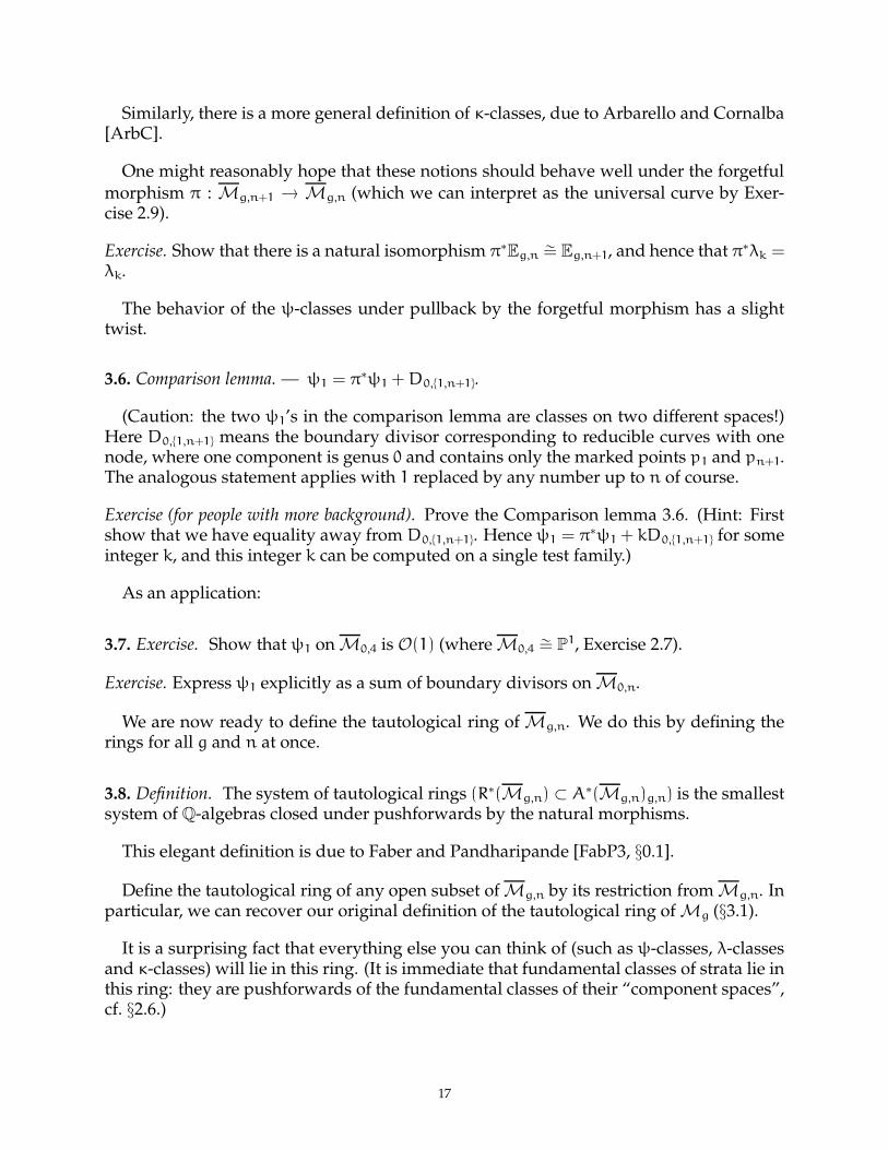
Similarly, there is a more general definition of κ-classes, due to Arbarello and Cornalba[ArbC].

One might reasonably hope that these notions should behave well under the forgetfulmorphism π : Mg,n+1 → Mg,n (which we can interpret as the universal curve by Exer-cise 2.9).

Exercise. Show that there is a natural isomorphism π∗Eg,n∼= Eg,n+1, and hence that π∗λk =

λk.

The behavior of the ψ-classes under pullback by the forgetful morphism has a slighttwist.

3.6. Comparison lemma. — ψ1 = π∗ψ1 +D0,1,n+1.

(Caution: the two ψ1’s in the comparison lemma are classes on two different spaces!)Here D0,1,n+1 means the boundary divisor corresponding to reducible curves with onenode, where one component is genus 0 and contains only the marked points p1 and pn+1.The analogous statement applies with 1 replaced by any number up to n of course.

Exercise (for people with more background). Prove the Comparison lemma 3.6. (Hint: Firstshow that we have equality away from D0,1,n+1. Hence ψ1 = π∗ψ1 + kD0,1,n+1 for someinteger k, and this integer k can be computed on a single test family.)

As an application:

3.7. Exercise. Show that ψ1 on M0,4 is O(1) (where M0,4∼= P1, Exercise 2.7).

Exercise. Express ψ1 explicitly as a sum of boundary divisors on M0,n.

We are now ready to define the tautological ring of Mg,n. We do this by defining therings for all g and n at once.

3.8. Definition. The system of tautological rings (R∗(Mg,n) ⊂ A∗(Mg,n)g,n) is the smallestsystem of Q-algebras closed under pushforwards by the natural morphisms.

This elegant definition is due to Faber and Pandharipande [FabP3, §0.1].

Define the tautological ring of any open subset of Mg,n by its restriction from Mg,n. Inparticular, we can recover our original definition of the tautological ring of Mg (§3.1).

It is a surprising fact that everything else you can think of (such as ψ-classes, λ-classesand κ-classes) will lie in this ring. (It is immediate that fundamental classes of strata lie inthis ring: they are pushforwards of the fundamental classes of their “component spaces”,cf. §2.6.)

17

We next give an equivalent description of the tautological groups, which will be conve-nient for many of our arguments, because we do not need to make use of the multiplica-tive structure. In this description, the ψ-classes play a central role.

3.9. Definition [GrV3, Defn. 4.2]. The system of tautological rings (R∗(Mg,n) ⊂ A∗(Mg,n)g,n)

is the smallest system of Q-vector spaces closed under pushforwards by the natural mor-phisms, such that all monomials in ψ1, . . . , ψn lie in R∗(Mg,n).

The equivalence of Definition 3.8 and Definition 3.9 is not difficult (see for example[GrV3]).

3.10. Faber-type conjectures for Mg,n, and the conjecture of Hain-Looijenga-Faber-Pandharipande.

In analogy with Faber’s conjecture, we have the following.

3.11. Conjecture. R∗(Mg,n) is a Poincare-duality ring of dimension 3g− 3+ n.

This was first asked as a question by Hain and Looijenga [HLo, Question 5.5], firststated as a speculation by Faber and Pandharipande [FabP1, Speculation 3] (in the casen = 0), and first stated as a conjecture by Pandharipande [P, Conjecture 1]. In analogywith Faber’s conjecture, we break this into two parts.

I. “Socle” conjecture. R3g−3+n(Mg,n) ∼= Q. This is obvious if we define the tautologicalring in terms of cohomology: H2(3g−3+n)(Mg,n) ∼= Q, and the zero-dimensional stratashow that the tautological zero-cycles are not all zero. However, in the tautological Chowring, the socle conjecture is not at all obvious. Moreover, the conjecture is not true in thefull Chow ring — A0(M1,11) is uncountably generated, while the conjecture states thatR0(M1,11) has a single generator. (By R0, we of course mean R3g−3+n.)

We will prove the vanishing conjecture in §4.6.

II. Perfect pairing conjecture For 0 ≤ i ≤ 3g− 3+ n, the natural product

Ri(Mg,n) × R3g−3+n−i(Mg,n) → R3g−3+n(Mg,n) ∼= Q

is a perfect pairing. (We currently have no idea why this should be true.)

Hence, in analogy with Faber’s conjecture, if this conjecture were true, then we couldrecover the entire ring by knowing the top intersections. This begs the question of how tocompute all top intersections.

3.12. Fact/recipe (Mumford and Faber). If we knew the top intersections of ψ-classes,we would know all top intersections. In other words, there is an algorithm to compute alltop intersections if we knew the numbers

(5)

∫

Mg,n

ψa1

1 · · ·ψan

n ,∑

ai = 3g− 3+ n.

18

(This is a worthwhile exercise for people with some familiarity with the moduli spaceof curves.) This is the basis of Faber’s wonderful computer program [Fab2] computingtop intersections of various tautological classes. For more information, see [Fab3]. Thisconstruction is useful in understanding the definition (Defn. 3.9) of the tautological groupin terms of the ψ-classes.

Until a key insight of Witten’s, there was no a priori reason to expect that these numbersshould behave nicely. We will survey three methods of computing these numbers: (i)partial results in low genus; (ii) Witten’s conjecture; and (iii) via the ELSV formula. Afourth (attractive) method was given in Kevin Costello’s thesis [C].

3.13. Top intersections on Mg,n: partial results in low genus. Here are two crucial relationsamong top intersections.

Dilaton equation. If Mg,n exists (i.e. there are stable n-pointed genus g curve, or equiva-lently 2g− 2+ n > 0), then

∫

Mg,n+1

ψβ1

1 · · ·ψβ2

2 · · ·ψβn

n ψn+1 = (2g− 2+ n)

∫

Mg,n

ψβ1

1 · · ·ψβn

n .

String equation. If 2g− 2+ n > 0, then

∫

Mg,n+1

ψβ1

1 ψβ2

2 · · ·ψβn

n =

n∑

i=1

∫

Mg,n

ψβ1

1 ψβ2

2 · · ·ψβi−1i · · ·ψβn

n

(where you ignore terms where you see negative exponents).

Exercise (for those with more experience). Prove these using the Comparison lemma 3.6.

Equipped with the string equation alone, we can compute all top intersections in genus

0, i.e.∫M0,n

ψβ1

1 · · ·ψβnn where

∑βi = n − 3. (In any such expression, some βi must be

0, so the string equation may be used.) Thus we can recursively solve for these numbers,starting from the base case

∫M0,3

∅ = 1.

Exercise. Show that ∫

M0,n

ψa1

1 · · ·ψan

n =

(

n− 3

a1, · · · , an

)

.

In genus 1, the story is similar. In this case, we need both the string and dilaton equa-tion.

Exercise. Show that any integral∫

M1,n

ψβ1

1 · · ·ψβn

n

can be computed using the string and dilaton equation from the base case∫M1,1

ψ1 =

1/24.

19

We now sketch why the base case∫M1,1

ψ1 = 1/24 is true. We calculate this by choosing

a finite cover P1 → M1,1. Consider a general pencil of cubics in the projective plane. Inother words, take two general homogeneous cubic polynomials f and g in three variables,and consider the linear combinations of f and g. The non-zero linear combinations mod-ulo scalars are parametrized by a P1. Thus we get a family of cubics parametrized by P1,i.e. C → P1.

You can verify that in this family, there will be twelve singular fibers, that are cubicswith one node. One way of verifying this is as follows: f = g = 0 consists of nine pointsp1, . . . , p9 (basically by Bezout’s theorem — you expect two cubics to meet at nine points).There is a map P2 − p1, . . . , p9 → P1. If C is the blow-up of P2 at the nine points, thenthis map extends to C → P1, and this is the total space of the family. The (topological)Euler characteristic of C is the Euler characteristic of P2 (which is 3) plus 9 (as each blow-up replaces a point by a P1), i.e. χ(C) = 12. Considering C as a fibration over P1, mostfibers are elliptic curves, which have Euler characteristic 0. Hence χ(C) is the sum of theEuler characteristics of the singular fibers. Each singular fiber is a nodal cubic, which isisomorphic to P1 with two points glued together (depicted in Figure 5); this is the unionof C∗ (which has Euler characteristic 0) with a point, so χ(C) is the number of singularfibers. (This argument needs further justification at every point!)

We have a section of C → P1, given by the exceptional fiber E of the blow-up of p1.Hence we have a moduli map µ : P1 → M1,1 of smooth curves. Clearly it doesn’t mapP1 to a point, as some of the fibers are smooth, and twelve are singular. Thus the modulimap µ is surjective (as the image is an irreducible closed set that is not a point). You mightsuspect that µ has degree 12, as the preimage of the boundary divisor ∆ ∈ M1,1 has 12preimages, and one can check that µ is nonsingular here. However, we come to one ofthe twists of stack theory — each point of M1,1, including ∆, has degree 1/2— each pointshould be counted with multiplicity one over the size its automorphism group, and each1-pointed genus 1 stable curve has precisely one nontrivial automorphism.

Thus 24∫M1,1

ψ1 =∫

P1 µ∗ψ1, so we wish to show that

∫P1 µ

∗ψ1 = 1. This is an explicit

computation on C → P1. You may check that on the blow-up to C, the dualizing sheaf tothe fiber at p1 is given by −O(E)|E. As E2 = −1, we have

∫P1 µ

∗ψ1 = −E2 = 1 as desired.

In higher genus, the string and dilaton equation are also very useful.

Exercise. Fix g. Show that using the string and dilaton equation, all of the numbers (5)(for all n) can be computed from a finite number of base cases. The number of base casesrequired is the number of partitions of 3g− 3. (It is useful to describe this more precisely,by explicitly describing the generating function for (5) in terms of these base cases.)

3.14. Witten’s conjecture. So how do we get at these remaining base cases? The answer wasgiven by Witten [W]. (This presentation is not chronological — Witten’s conjecture camefirst, and motivated most of what followed. In particular, it predates Faber’s conjectures,and was used to generate the data that led Faber to his conjectures.)

20

Witten’s conjecture (Kontsevich’s theorem). Let

Fg =∑

n≥0

1

n!

∑

k1,...,kn

(∫

Mg,n

ψk1

1 · · ·ψkn

n

)

tk1· · · tkn

be the generating function for the genus g numbers (5), and and let

F =∑

Fgh2g−2

be the generating function for all genus. (This is Witten’s free energy, or the Gromov-Wittenpotential of a point.) Then

(2n+ 1)∂3

∂tn∂t20

F =

(

∂2

∂tn−1∂t0F

)(

∂3

∂t30F

)

+ 2

(

∂3

∂tn−1∂t20

F

)(

∂2

∂t20F

)

+1

4

∂5

∂tn−1∂t40

F.

Witten’s conjecture now has many proofs, by Kontsevich [Ko1], Okounkov-Pandharipande[OP], Mirzakhani [Mi], and Kim-Liu [KiL]. It is a sign of the richness of this conjecturethat these proofs are all very different, and all very enlightening in different ways.

The reader should not worry about the details of this formula, and should just look atits shape. Those familiar with integrable systems will recognize this as the Korteweg-deVries (KdV) equation, in some guise. There was a later reformulation due to Dijkgraaf,Verlinde, and Verlinde [DVV], in terms of the Virasoro algebra. Once again, the readershould not worry about the precise statement, and concentrate on the form of the conjec-ture. Define differential operators (n ≥ −1)

L−1 = −∂

∂t0+h−2

2t20 +

∞∑

i=0

ti+1

∂

∂ti

L0 = −3

2

∂

∂t1+

∞∑

i=0

2i+ 1

2ti∂

∂ti+1

16

Ln =

∞∑

k=0

Γ(m+ n+ 32)

Γ(k+ 12)

(tk − δk,1)δn+k +h2

2

n−1∑

k=1

(−1)k+1Γ(n− k+ 1

2)

Γ(−k− 12)δkδn−k−1 (n > 0)

These operators satisfy [Lm, Ln] = (m− n)Lm+n.

Exercise. Show that L−1eF = 0 is equivalent to the string equation. Show that L0e

F = 0 isequivalent to the dilaton equation.

Witten’s conjecture is equivalent to: LneF = 0 for all n. These equations let you induc-

tively solve for the co-efficients of F, and hence compute all these numbers.

3.15. The Virasoro conjecture. The Virasoro formulation of Witten’s conjecture has a far-reaching generalization, the Virasoro conjecture described earlier. Instead of top intersec-tions on the moduli space of curves, it addresses top (virtual) intersections on the modulispace of maps of curves to some space X. Givental’s proof (to be explicated by Lee andPandharipande) for the case of projective space (and more generally Fano toric varieties)was mentioned earlier. It is also worth mentioning Okounkov and Pandharipande’s proofin the case where X is a curve; this is also a tour-de-force.

21

3.16. Hurwitz numbers and the ELSV formula. We can also recover these top intersectionsvia the old-fashioned theme of branched covers of the projective line, the very techniquethat let us compute the dimension of the moduli space of curves, and of the Picard variety§2.2.

Fix a genus g, a degree d, and a partition of d into n parts, α1 + · · ·+ αn = d, which wewrite as α ` d. Let

(6) r := 2g+ d+ n− 2.

Fix r + 1 points p1, . . . , pr,∞ ∈ P1. Define the Hurwitz number Hgα to be the number of

branched covers of P1 by a Riemann surface, that are unbranched away from p1, . . . , pr,∞,such that the branching over ∞ is given by α1, . . . , αn (i.e. there are n preimages of ∞, andthe branching at the ith preimage is of order αi, i.e. the map is analytically locally givenby t 7→ tαi ), and there is the simplest possible branching over each pi, i.e. the branchingis given by 2 + 1 + · · · + 1 = d. (To describe this simple branching more explicitly: aboveany such branch point, d− 2 of the sheets are unbranched, and the remaining two sheetscome together. The analytic picture of the two sheets is the projection of the parabolay2 = x to the x-axis in C2.) We consider the n preimages of ∞ to be labeled. Caution:in the literature, sometimes the preimages of ∞ are not labeled; that definition of Hurwitznumber will be smaller than ours by a factor of # Autα, where Autα is the subgroup ofSn fixing the n-tuple (α1, . . . , αn) (e.g. if α = (2, 2, 2, 5, 5), then # Autα = 3!2!).

One technical point: each cover is counted with multiplicity 1 over the size of the auto-morphism group of the cover.

Exercise. Use the Riemann-Hurwitz formula (2) to show that if the cover is connected,then it has genus g.

Experts will recognize these as relative descendant Gromov-Witten invariants of P1;we will discuss relative Gromov-Witten invariants of P1 in Section 5. However, they aresomething much more down-to-earth. The following result shows that this number is apurely combinatorial object. In particular, there are a finite number of such covers.

3.17. Proposition. —

Hgα = #

(σ1, . . . , σr) : σi transpositions generating Sd,

r∏

i=1

σi ∈ C(α)

# Autα/d!,

where the σi are transpositions generating the symmetric group Sd, and C(α) is the conjugacyclass in Sd corresponding to partition α.

Before we give the proof, we make some preliminary comments. As an example, con-sider d = 2, α = 2, g arbitrary, so r = 2g + 1. The above formula gives Hg

α = 1/2, whichat first blush seems like nonsense — how can we count covers and get a non-integer?Remember however the combinatorial/stack-theoretic principal that objects should becounted with multiplicity 1 over the size of their automorphism group. Any double coverof this sort always has a non-trivial involution (the “hyperelliptic involution”). Hencethere is indeed one cover, but it is counted as “half a cover”. Fortunately, this is the only

22

case of Hurwitz numbers for which this is an issue. The reader may want to follow thisparticular case through in the proof.

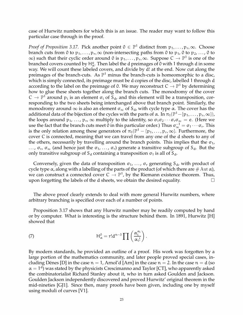
Proof of Proposition 3.17. Pick another point 0 ∈ P1 distinct from p1, . . . , pr,∞. Choosebranch cuts from 0 to p1, . . . , pr,∞ (non-intersecting paths from 0 to p1, 0 to p2, . . . , 0 to∞) such that their cyclic order around 0 is p1, . . . , pr,∞. Suppose C → P1 is one of thebranched covers counted byHg

α. Then label the d preimages of 0with 1 through d in someway. We will count these labeled covers, and divide by d! at the end. Now cut along thepreimages of the branch-cuts. As P1 minus the branch-cuts is homeomorphic to a disc,which is simply connected, its preimage must be d copies of the disc, labelled 1 through daccording to the label on the preimage of 0. We may reconstruct C → P1 by determininghow to glue these sheets together along the branch cuts. The monodromy of the coverC → P1 around pi is an element σi of Sd, and this element will be a transposition, cor-responding to the two sheets being interchanged above that branch point. Similarly, themonodromy around ∞ is also an element σ∞ of Sd, with cycle type α. The cover has theadditional data of the bijection of the cycles with the parts of α. In π1(P

1− p1, . . . , pr,∞),the loops around p1, . . . , pr, ∞ multiply to the identity, so σ1σ2 · · ·σrσ∞ = e. (Here weuse the fact that the branch cuts meet 0 in this particular order.) Thus σ−1

∞ = σ1 · · ·σr. Thisis the only relation among these generators of π1(P

1 − p1, . . . , pr,∞. Furthermore, thecover C is connected, meaning that we can travel from any one of the d sheets to any ofthe others, necessarily by travelling around the branch points. This implies that the σ1,. . . , σr, σ∞ (and hence just the σ1, . . . , σr) generate a transitive subgroup of Sd. But theonly transitive subgroup of Sd containing a transposition σ1 is all of Sd.

Conversely, given the data of transposition σ1, . . . , σr generating Sd, with product ofcycle type α, along with a labelling of the parts of the product (of which there are # Autα),we can construct a connected cover C → P1, by the Riemann existence theorem. Thus,upon forgetting the labels of the d sheets, we obtain the desired equality.

The above proof clearly extends to deal with more general Hurwitz numbers, wherearbitrary branching is specified over each of a number of points.

Proposition 3.17 shows that any Hurwitz number may be readily computed by handor by computer. What is interesting is the structure behind them. In 1891, Hurwitz [H]showed that

(7) H0α = r!dn−3

∏(

ααi

i

αi!

)

.

By modern standards, he provided an outline of a proof. His work was forgotten by alarge portion of the mathematics community, and later people proved special cases, in-cluding Denes [D] in the case n = 1, Arnol’d [Arn] in the case n = 2. In the case n = d (soα = 1d) was stated by the physicists Crescimanno and Taylor [CT], who apparently askedthe combinatorialist Richard Stanley about it, who in turn asked Goulden and Jackson.Goulden Jackson independently discovered and proved Hurwitz’ original theorem in themid-nineties [GJ1]. Since then, many proofs have been given, including one by myselfusing moduli of curves [V1].

23

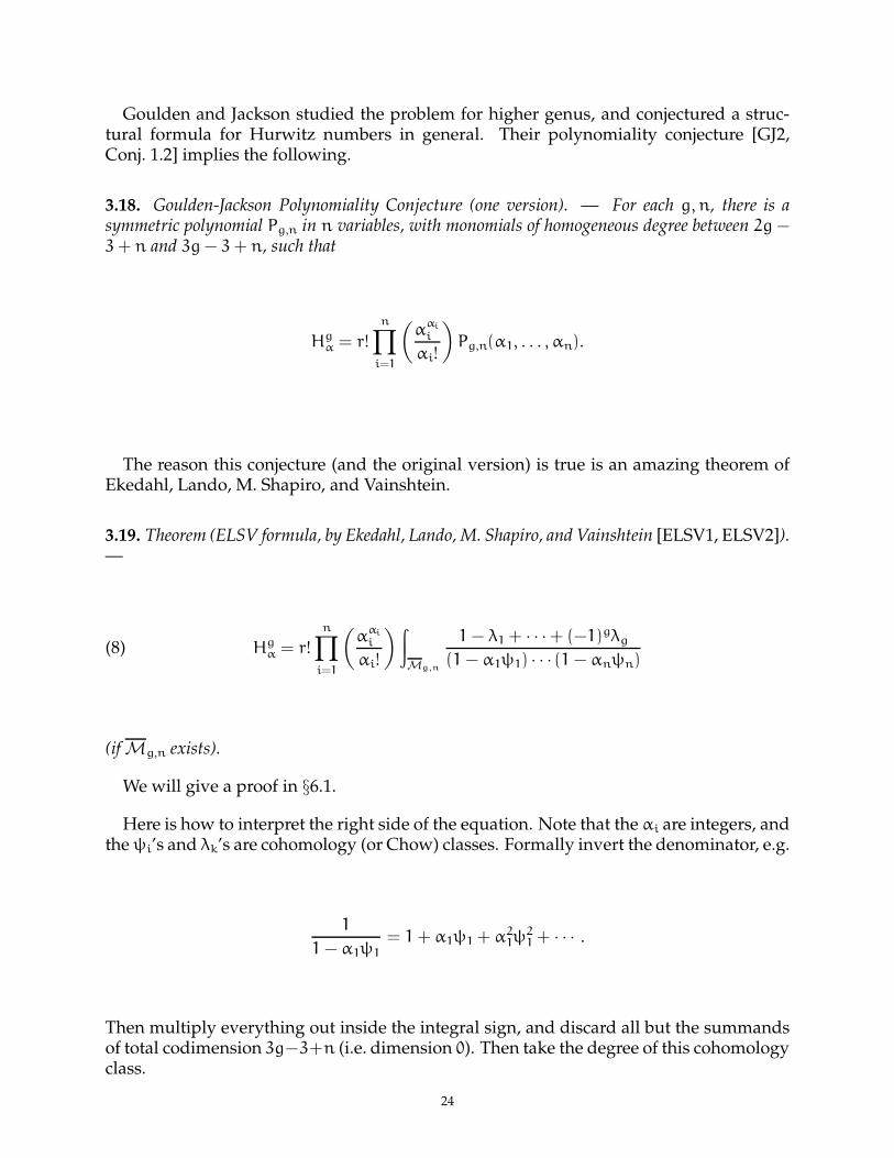
Goulden and Jackson studied the problem for higher genus, and conjectured a struc-tural formula for Hurwitz numbers in general. Their polynomiality conjecture [GJ2,Conj. 1.2] implies the following.

3.18. Goulden-Jackson Polynomiality Conjecture (one version). — For each g, n, there is asymmetric polynomial Pg,n in n variables, with monomials of homogeneous degree between 2g −

3+ n and 3g− 3+ n, such that

Hgα = r!

n∏

i=1

(

ααi

i

αi!

)

Pg,n(α1, . . . , αn).

The reason this conjecture (and the original version) is true is an amazing theorem ofEkedahl, Lando, M. Shapiro, and Vainshtein.

3.19. Theorem (ELSV formula, by Ekedahl, Lando, M. Shapiro, and Vainshtein [ELSV1, ELSV2]).—

(8) Hgα = r!

n∏

i=1

(

ααi

i

αi!

) ∫

Mg,n

1− λ1 + · · ·+ (−1)gλg

(1− α1ψ1) · · · (1− αnψn)

(if Mg,n exists).

We will give a proof in §6.1.

Here is how to interpret the right side of the equation. Note that the αi are integers, andtheψi’s and λk’s are cohomology (or Chow) classes. Formally invert the denominator, e.g.

1

1− α1ψ1

= 1+ α1ψ1 + α21ψ

21 + · · · .

Then multiply everything out inside the integral sign, and discard all but the summandsof total codimension 3g−3+n (i.e. dimension 0). Then take the degree of this cohomologyclass.

24

For example, if g = 0 and n = 4, we get

Hgα = r!

4∏

i=1

(

ααi

i

αi!

) ∫

M0,4

1− λ1 + · · · ± λg

(1− α1ψ1) · · · (1− α4ψ4)

= r!

4∏

i=1

(

ααi

i

αi!

) ∫

M0,4

(1+ α1ψ1 + · · · ) · · · (1+ α4ψ4 + · · · )

= r!

4∏

i=1

(

ααi

i

αi!

) ∫

M0,4

(α1ψ1 + · · ·+ α4ψ4)

= r!

4∏

i=1

(

ααi

i

αi!

)

(α1 + · · ·+ α4) (Exercise 3.7)

= r!

4∏

i=1

(

ααi

i

αi!

)

d.

Exercise. Recover Hurwitz’ original formula (7) from the ELSV-formula, at least if n ≥ 3.

More generally, expanding the integrand of (8) yields

(9)∑

a1+···+an+k=3g−3+n

(

(−1)k

(∫

Mg,n

ψa1

1 · · ·ψan

n λk

))

(αa1

1 · · ·αan

n ) .

This is a polynomial in α1, . . . , αn of homogeneous degree between 2g − 3 + n and 3g −

3 + n. Thus this explains the mystery polynomial in the Goulden-Jackson PolynomialityConjecture 3.18 — and the coefficients turn out to be top intersections on the modulispace of curves! (The original polynomiality conjecture was actually different, and sometranslation is necessary in order to make the connection with the ELSV formula [GJV1].)

There are many other consequences of the ELSV formula; see [ELSV2, GJV1] for sur-veys.

We should take a step back to see how remarkable the ELSV formula is. To any reason-able mathematician, Hurwitz numbers (as defined by Proposition 3.17) are purely dis-crete, combinatorial objects. Yet their structure is fundamentally determined by topologyof the moduli space of curves. Put more strikingly — the combinatorics of transpositionsin the symmetric group lead inexorably to the tautological ring of the moduli space ofcurves!

3.20. We return to our original motivation for discussing the ELSV formula: computingtop intersections of ψ-classes on the moduli space of curves Mg,n. Fix g and n. As statedearlier, any given Hurwitz number may be readily computed (and this can be formal-ized elegantly in the language of generating functions). Thus any number of values ofPg,n(α1, . . . , αn) may be computed. However, we know that Pg,n is a symmetric poly-nomial of known degree, and it is straightforward to show that one can determine theco-efficients of a polynomial of known degree from enough values. In particular, from

25

(9), the coefficients of the highest-degree terms in Pg,n are precisely the top intersectionsof ψ-classes.

This is a powerful perspective. As an important example, Okounkov and Pandhari-pande used the ELSV formula to prove Witten’s conjecture.

3.21. Back to Faber-type conjectures.

This concludes our discussion of Faber-type conjectures for Mg,n. I have two moreremarks about Faber-type conjectures. The first is important, the second a side-remark.

3.22. Faber’s intersection number conjecture on Mg, take two. We define the moduli spaceof n-pointed genus g curves with “rational tails”, denoted Mrt

g,n, as follows. We define

Mrtg,n as the dense open subset of Mg,n parametrizing pointed nodal curves where one

component is nonsingular of genus g (and the remaining components form trees of genus0 curves sprouting from it — hence the phrase “rational tails”). If g > 1, then Mrt

g,n =

π−1(Mg), where π : Mg,n → Mg is the forgetful morphism. Note that Mrtg = Mg.

We may restate Faber’s intersection number conjecture (for Mg) in terms of this modulispace. By our re-definition of the tautological ring on Mg in §3.3 (Definition 3.9, using alsoFaber’s constructions of §3.12), the “top intersections” are determined by π∗ψ

a1

1 · · ·ψann

(where π : Mrtg,n → Mg) for

∑ai = g− 2+ n.

Then Faber’s intersection number conjecture translates to the following.

3.23. Faber’s intersection number conjecture (take two). — If all αi > 1, then

ψα1

1 · · ·ψαn

n =(2g− 3+ k)!(2g− 1)!!

(2g− 1)!∏k

j=1(2dj + 1)!![generator] for

∑αi = g− 2+ n

where [generator] = κg−2 = π∗ψg−11 .

(This reformulation is also due to Faber.) This description is certainly more beautifulthan the original one (4), which suggests that we are closer to the reason for it to be true.

3.24. The other conjectures of Faber were extended to Mrtg,n by Pandharipande [P, Conj.

1].

3.25. Remark: Faber-type conjectures for curves of compact type. Based on the cases of theMg and Mg,n, Faber and Pandharipande made another conjecture for curves of “compacttype”. A curve is said to be of compact type if its Jacobian is compact, or equivalently ifits dual graph has no loops, or equivalently, if the curve has no nondisconnecting nodes.Define Mc

g,n ⊂ Mg,n to be the moduli space of curves of compact type. It is Mg,n minusan irreducible divisor, corresponding to singular curves with one irreducible component(called ∆0, although we will not use this notation).

26

1

FIGURE 5. The curve corresponding to the point δ0 ∈ M1,1

3.26. Conjecture (Faber-Pandharipande [FabP1, Spec. 2], [P, Conj. 1]. — R∗(Mcg) is a Poincare

duality ring of dimension 2g− 3.

Again, this has a vanishing/socle part and a perfect pairing part. There is something thatcan be considered the corresponding intersection number part, Pandharipande and Faber’sλg theorem [FabP2].

We will later (§4.7) give a proof of the vanishing/socle portion of the conjecture, thatRi(Mc

g) = 0 for i > 2g − 3, and is 1-dimensional if i = 2g − 3. The perfect pairing part isessentially completely open.

3.27. Other relations in the tautological ring.

We have been concentrating on top intersections in the tautological ring. I wish todiscuss more about other relations (in smaller codimension) in the tautological ring.

In genus 0, as stated earlier (§3.4), all classes on Mg,n are generated by the strata, andthe only relation among them are the cross-ratio relations. We have also determined theψ-classes in terms of the boundary classes.

In genus 1, we can verify that ψ1 can be expressible in terms of boundary strata. OnM1,1, if the boundary point is denoted δ0 (the class of the nodal elliptic curve shown inFigure 5), we have shown ψ1 = δ0/12. (Reason: we proved it was true on a finite cover,in the course of showing that

∫M1,1

ψ1 = 1/24.) We know how to pull back ψ-classes by

forgetful morphisms, so we can now verify the following.

Exercise. Show that in the cohomology group of M1,n, ψi is equivalent to a linear combi-nation of boundary divisors. (Hint: use the Comparison Lemma 3.6.)

3.28. Slightly trickier exercise. Use the above to show that the tautological ring in genus 1is generated (as a group) by boundary classes. (This fact was promised in §3.4.)

In genus 2, this is no longer true: ψ1 is not equivalent to a linear combination of bound-ary strata on M2,1. However, in 1983, Mumford showed that ψ2

1 (on M2,1) is a combina-tion of boundary strata ([Mu], see also [Ge2, eqn. (4)]); in 1998, Getzler showed the same

27

2

ψ

5

4

2

6

1

3

FIGURE 6. A class on M2,6 — a codimension 1 class on a boundary stratum,constructed using ψ1 on M2,3 and gluing morphisms

for ψ1ψ2 (on M2,2) [Ge2]. These two results can be used to show that on M2,n, all tauto-logical classes are linear combinations of strata, and from classes “constructed using ψ1

on M2,1”. Figure 6 may help elucidate what classes we mean — they correspond to dualgraphs, with at most one marking ψ on an edge incident to one genus 2 component. Theclass in question is defined by gluing together the class of ψi on M2,v corresponding tothat genus 2 component (where v is the valence, and i corresponds to the edge labeled byψ) with the fundamental classes of the M0,vj

’s corresponding to the other vertices. Thequestion then arises: what are the relations among these classes? On top of the cross-ratioand Getzler relation, there is a new relation due to Belorousski and Pandharipande, incodimension 2 on M2,3 [BP]. We do not know if these three relations generate all therelations. (All the genus 2 relations mentioned in this paragraph are given by explicitformulas, although they are not pretty to look at.)

In general genus, the situation should get asymptotically worse as g grows. However,there is a general statement that can be made:

3.29. Getzler’s conjecture [Ge2, footnote 1] (Ionel’s theorem [I1]). — If g > 0, all degree gpolynomials in ψ-classes vanish on Mg,n (hence live on the boundary on Mg,n).

We will interpret this result as a special case of a more general result (Theorem ?), in§4.3. In keeping with the theme of this article, the proof will be Gromov-Witten theoretic.

3.30. Y.-P. Lee’s Invariance Conjecture. There is another general statement that may wellgive all the relations in every genus: Y.-P. Lee’s Invariance conjecture. It is certainly cur-rently beyond our current ability to either prove it. Lee’s conjecture is strongly motivatedby Gromov-Witten theory.

Before we state the conjecture, we discuss the consequences and evidence. All of theknown relations in the tautological rings are consequences of the conjecture. For example,the genus 2 implications are shown by Arcara and Lee in [ArcL1]. They then predicteda new relation in M3,1 in [ArcL2]. Simultaneously and independently, this relation wasproved by Kimura and X. Liu [KL]. This seems to be good evidence for the conjecturebeing true.

28

More recently, the methods behind the conjecture have allowed Lee to turn these pre-dictions into proofs, not conditional on the truth of the conjecture [Lee2]. Thus for exampleArcara and Lee’s work yields a proof of the new relation on M3,1.

We now give the statement. The conjecture is most naturally expressed in terms ofthe tautological rings of possibly-disconnected curves. The definition of a stable possibly-disconnected curve is the same as that of a stable curve, except the curve is not requiredto be connected. We denote the moduli space of n-pointed genus g possibly-disconnected

curves by M•

g,n. The reader can quickly verify that our discussion of the moduli spaceof curves carries over without change if we consider possibly-disconnected curves. For

example, M•

g,n is nonsingular and pure-dimensional of dimension 3g − 3 + n (although

not in general irreducible). It contains Mg,n as a component, so any statements about

M•

g,n will imply statements about Mg,n. Note that the disjoint union of two curves ofarithmetic genus g and h is a curve of arithmetic genus g + h − 1: Euler characteristicsadd under disjoint unions. Note also that a possibly-disconnected marked curve is stableif and only if all of its connected components are stable.

Exercise. Show that M•

−1,6 is a union of(

6

3

)

/2 points — any 6-pointed genus −1 stablecurve must be the disjoint union of two P1’s, with 3 of the 6 labeled points on each com-ponent.

Exercise. Show that any component of M•

g,n is the quotient of a product of Mg′,n′’s by afinite group.

Tautological classes are generated by classes corresponding to a dual graph, with each

vertex (of genus g and valence n, say) labeled by some cohomology class on M•

g,n (pos-sibly the fundamental class); call this a decorated dual graph. (We saw an example of adecorated dual graph in Figure 6. Note that ψ-classes will always be associated to somehalf edge.) Decorated dual graphs are not required to be connected. If Γ is a decorateddual graph (of genus gwith n tails, say), let dim Γ be the dimension of the corresponding

class in A∗(M•

g,n).

For each positive integer l, we will describe a linear operator rl that sends formal lin-ear combinations of decorated dual graphs to formal linear combinations of decorateddual graphs. It is homogeneous of degree −l: it sends (dual graphs corresponding to)dimension k classes to (dual graphs corresponding to) dimension k− l classes.

We now describe its action on a single decorated dual graph Γ of genus gwith nmarkedpoints (or half-edges), labeled 1 through n. Then rl(Γ) will be a formal linear combinationof other graphs, each of genus g− 1with n+ 2 marked points.

There are three types of contributions to rlΓ . (In each case, we discard any graph that isnot stable.)

1. Edge-cutting. There are two contributions for each directed edge, i.e. an edge with chosenstarting and ending point. (Caution: there are two possible directions for each edge ingeneral, except for those edges that are “loops”, connecting a single vertex to itself. In this

29

case, both directions are considered the same.) We cut the edge, regarding the two half-edges as “tails”, or marked points. The starting half-edge is labeled n+ 1, and the endinghalf-edge is labeled n + 2. One summand will correspond to adding an extra decorationof ψl to point n + 1. (In other words, ψl

n+1 is multiplied by whatever cohomology classis already decorating that vertex.) A second summand will correspond to the adding anextra decoration ofψl to point n+2, and this summand appears with multiplicity (−1)l−1.

2. Genus reduction For each vertex we produce l graphs as follows. We reduce the genus ofthe vertex by 1, and add two new tails to this vertex, labelled n+1 and n+2; we decoratethem with ψm and ψl−1−m respectively, where 0 ≤ m ≤ l − 1. Each such graph is takenwith multiplicity (−1)m+1.

3. Vertex-splitting. For each vertex, we produce a number of graphs as follows. We splitthe vertex into two, and the first new vertex is given the tail n+1, and the second is giventhe tail n + 2. The two new tails are decorated by ψm and ψl−1−m respectively, where0 ≤ m ≤ l − 1. We then take one such graph for each choice of splitting of the genusg = g1 + g2 and partitioning of the other incident edges. Each such graph is taken withmultiplicity (−1)m+1.

Then rl(Γ) is the sum of the above summands. Observe that when l is odd (resp. even),the result is symmetric (resp. anti-symmetric) in labels n + 1 and n + 2.

By linearity, this defines the action of rl on any linear combination of directed graphs.

3.31. Y.-P. Lee’s Invariance Conjecture [Lee1, Conj. 1–2]. —

(a) If∑ciΓi = 0 holds in A∗(M

•

g,n), then rl(∑ciΓi) = 0 in A∗(Mg−1,n+2).

(b) Conversely, if∑ciΓi has positive pure dimension, and rl(

∑ciΓi) = 0 inA∗(Mg−1,n+2),

then∑ciΓi = 0 holds in A∗(M

•

g,n).

This can be used to produce tautological equations inductively! The base case is when

dimM•

g,n = 0, which is known: we will soon show (§4.6) that R0(Mg,n) ∼= Z, and hence

dimension 0 tautological classes on Mg,n are determined by their degree (and dimension

0 tautological classes on M•

g,n are determined by their degree on each connected compo-

nent). Note that the algorithm is a finite process: the dimension l relations on Mg,n or

M•

g,n produced by this algorithm are produced after a finite number of steps.

Even more remarkably, this seems to produce all tautological relations:

3.32. Y.-P. Lee’s Invariance Conjecture, continued [Lee1, Conj. 3]. — Conjecture 3.31(b) willproduce all tautological equations inductively.

A couple of remarks are in order. Clearly this is a very combinatorial description. Itwas dictated by Gromov-Witten theory, as explained in [Lee1]. In particular, it uses the

30

fact that all tautological equations are invariant under the action of lower triangular sub-groups of the twisted loop groups, and proposes that they are the only equations invariantin this way.

In order to see the magic of this conjecture in action, and to get experience with therl operators, it is best to work out an example. The simplest dimension 1 relation is thefollowing.

Exercise. Show that the pullback of the (dimension 0) cross-ratio relation (§3.4) on M0,4 toa (dimension 1) relation on M0,5 is implied by the Invariance Conjecture. (Some ratherbeautiful cancellation happens.)

4. A BLUNT TOOL: THEOREM ? AND CONSEQUENCES

We now describe a blunt tool from which much of the previously described structureof the tautological ring follows. Although it is statement purely about the stratification ofthe moduli space of curves, we will see (§6.3) that it is proved via Gromov-Witten theory.

4.1. Theorem ? [GrV3]. — Any tautological class of codimension i is trivial away from stratasatisfying

# genus 0 vertices ≥ i− g+ 1.

(Recall that the genus 0 vertices correspond to components of the curve with geometricgenus 0.)

More precisely, any tautological class is zero upon restriction to the (large) open setcorresponding to the open set corresponding to

# genus 0 vertices < i− g+ 1.

Put another way: given any tautological class of codimension i, you can move it intothe set of curves with at least i − g + 1 genus 0 components. A third formulation is thatthe tautological classes of codimension i are pushed forward from classes on the locus ofcurves with at least i− g+ 1 genus 0 components.

We remark that this is false for the Chow ring as a whole — this is fundamentally astatement about tautological classes.

We will discuss the proof in §6.3, but first we give consequences. There are in somesense four morals of this result.

First, this is the fundamental geometry behind many of the theorems we have been dis-cussing. We will see that they follow from Theorem ? by straightforward combinatorics.As a sign of this, we will often get strengthenings of what was known or conjecturedpreviously.

31

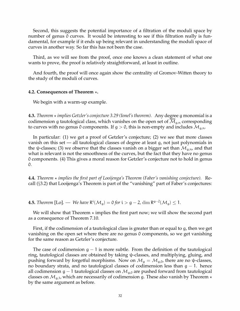
Second, this suggests the potential importance of a filtration of the moduli space bynumber of genus 0 curves. It would be interesting to see if this filtration really is fun-damental, for example if it ends up being relevant in understanding the moduli space ofcurves in another way. So far this has not been the case.

Third, as we will see from the proof, once one knows a clean statement of what onewants to prove, the proof is relatively straightforward, at least in outline.

And fourth, the proof will once again show the centrality of Gromov-Witten theory tothe study of the moduli of curves.

4.2. Consequences of Theorem ?.

We begin with a warm-up example.

4.3. Theorem ? implies Getzler’s conjecture 3.29 (Ionel’s theorem). Any degree gmonomial is acodimension g tautological class, which vanishes on the open set of Mg,n correspondingto curves with no genus 0 components. If g > 0, this is non-empty and includes Mg,n.

In particular: (1) we get a proof of Getzler’s conjecture; (2) we see that more classesvanish on this set — all tautological classes of degree at least g, not just polynomials inthe ψ-classes; (3) we observe that the classes vanish on a bigger set than Mg,n, and thatwhat is relevant is not the smoothness of the curves, but the fact that they have no genus0 components. (4) This gives a moral reason for Getzler’s conjecture not to hold in genus0.

4.4. Theorem ? implies the first part of Looijenga’s Theorem (Faber’s vanishing conjecture). Re-call (§3.2) that Looijenga’s Theorem is part of the “vanishing” part of Faber’s conjectures:

4.5. Theorem [Lo]. — We have Ri(Mg) = 0 for i > g− 2, dimRg−2(Mg) ≤ 1.

We will show that Theorem ? implies the first part now; we will show the second partas a consequence of Theorem 7.10.

First, if the codimension of a tautological class is greater than or equal to g, then we getvanishing on the open set where there are no genus 0 components, so we get vanishingfor the same reason as Getzler’s conjecture.

The case of codimension g − 1 is more subtle. From the definition of the tautologicalring, tautological classes are obtained by taking ψ-classes, and multiplying, gluing, andpushing forward by forgetful morphisms. Now on Mg = Mg,0, there are no ψ-classes,no boundary strata, and no tautological classes of codimension less than g − 1. henceall codimension g − 1 tautological classes on Mg,0 are pushed forward from tautologicalclasses on Mg,1, which are necessarily of codimension g. These also vanish by Theorem ?

by the same argument as before.

32

1

2

1 2

FIGURE 7. The 0-dimensional strata on M1,2 — notice that all vertices aregenus 0 and trivalent, and that there are 2g− 2+ n of them

As before, one can say more:

Exercise. Extend this argument to the moduli space of curves with rational tails we canextend Looijenga’s theorem to the moduli space of curves with rational tails Mrt

g,n. (Firstdetermine the dimension of the conjectural Poincare duality ring!)

The Faber-type conjecture for this space was mentioned in §3.24. I should point outthat I expect that Looijenga’s proof extends to this case without problem, but I haven’tchecked.

4.6. Theorem ? implies the socle part of Hain-Looijenga-Faber-Pandharipande conjecture 3.11 onMg,n. Recall the socle part of the Hain-Looijenga-Faber-Pandharipande conjecture 3.11,that R0(Mg,n) ∼= Q. (We write R3g−3+n(Mg,n) as R0(Mg,n) to remind the reader that thestatement is about tautological 0-cycles.)

We show how this is implied by Theorem ?. This was first shown in [GrV2], which canbe seen as a first step toward the statement and proof of Theorem ?.

Our goal is to show that all tautological 0-cycles are commensurate, and that one ofthem is non-zero. Clearly the latter is true, as the class of a 0-dimensional stratum (apoint) is tautological, and is non-zero as it has non-zero degree, so we concentrate on thefirst statement.

By Theorem ?, any dimension 0 tautological class is pushed forward from the locus ofcurves with at least (3g− 3+ n) − g+ 1 = 2g− 2+ n genus 0 components.

Exercise. Show that the only stable dual graphs with 2g−2+n genus 0 components has allvertices genus 0 and trivalent. Show that these are the 0-dimensional strata. (See Figure 7for the 0-dimensional strata on M1,2.)

Hence R0(Mg,n) is generated by these finite number of points. It remains to show thatany two of these points are equivalent in the Chow ring. A geometric way of showingthis is by observing that all points in M0,N are equivalent in the Chow ring, and thatour 0-dimensional strata are in the image of M0,2g+n under 2g gluing morphisms. Amore combinatorial way of showing this is by showing that each 1-dimensional stratumis isomorphic to P1, and that any two 0-dimensional strata can be connected by a chain of1-dimensional strata.

33

1

1

1

1

1

1

1 1

1

1 1

1

FIGURE 8. The two 0-pointed genus 6 stable trees with at least 4 genus 0 vertices

Exercise. Complete one of these arguments.

As in the earlier applications of Theorem ? too: we can verify that the perfect pairingconjecture in codimension 1 and probably 2 (although Tom Graber and I haven’t delvedtoo deeply into 2). This is combinatorially more serious, but not technically hard.

4.7. Theorem ? implies the Faber-Pandharipande vanishing/socle conjecture on curves of compacttype. We now show the “vanishing/socle part” of the Faber-type conjecture for curves ofcompact type (Faber-Pandharipande Conjecture 3.26).

First, suppose that i > 2g − 3. We will show that Ri(Mcg) = 0. By Theorem ?, any such

tautological class vanishes on the open set where there are at most i−g+ 1 > g− 2 genus0 vertices. Then our goal follows from the next exercise.

Exercise. Show that any genus g (0-pointed) stable graph that is a tree has at most g − 2

genus 0 vertices. Moreover, if equality holds, then each vertex is either genus 1 of valence1, or genus 0 of valence 3. (Examples when g = 6 are given in Figure 8.)

Next, if i = 2g− 3, then our codimension 2g− 3 (hence g) class is pushed forward fromstrata of the form described in the previous exercise. But each stratum has dimensiong, so the tautological class must be a linear combination of fundamental classes of suchstrata.

Furthermore, any two such strata are equivalent (in cohomology, or even in the Chowring) by arguments analogous to either of those we used for Mg,n.

Thus we have shown R2g−3(Mcg) is generated by the fundamental class of a single such

stratum. It remains to show that this is non-zero. This argument is short, but requiresa little more background than we have presented. (For the experts: it suffices to show

that λg 6= 0 on this stratum MΓ. We have a cover πMg

1,1 → MΓ via gluing morphisms,and the pullback of the Hodge bundle splits into the Hodge bundles of each of the gelliptic curves. Thus π∗λg is the product of the λ1-classes on each factor, so degπ∗λg =

(∫M1,1

λ1)g = 1/24g 6= 0.)

As always, Theorem ? gives extra information. (1) This argument extends to curves ofcompact type with points. (2) We can now attack part of the Poincare duality portion of

34

the conjecture. (3) We get an explicit generator of R2g−3(Mcg) (a stratum of a particular

form, e.g. Figure 8).

4.8. Theorem ? helps determine the tautological ring in low dimension. In the course of provingR0(Mg,n) ∼= Q, we showed that R0(Mg,n) was generated by 0-strata. A similar argumentshows that Ri(Mg,n) generated by boundary strata for i = 1, 2. (We are already awarethat this will not extend to i = 3, as ψ1 on M2,1 is the fundamental class of a stratum.)

In general, Theorem ? implies that in order to understand tautological classes in dimen-sion up to i, you need only understand curves of genus up to (i+1)/2, with not too manymarked points.

The moral of this is that the “top” (lowest-codimension) part of the tautological ringused to be considered the least mysterious (given the definition of the tautological ring, itis easy to give generators), and the bottom was therefore the most mysterious. Now thesituation is the opposite. For example, in codimension 3, we can describe the generatorsof the tautological ring, but we have no idea what the relations are. However, we knowexactly what the tautological ring looks like in dimension 3.

4.9. Exercise. Use Theorem ? and a similar argument to show that the tautological groupsof M0,n and M1,n are generated by boundary strata.

4.10. Additional consequences. For many additional consequences of Theorem ?, see[GrV3]. For example, we recover Diaz’ theorem (Mg contains no complete subvarieties

of dim > g − 2), as well as generalizations and variations such as: Mc

g,n contains nocomplete subvarieties of dim > 2g− 3+ n.

The idea behind the proof of Theorem ? is rather naive. But before we can discuss it,we will have to finally enter the land of Gromov-Witten theory, and define stable relativemaps to P1, which we will interpret as a generalization of the notion of a branched cover.

5. STABLE RELATIVE MAPS TO P1 AND RELATIVE VIRTUAL LOCALIZATION

We now discuss the theory of stable relative maps, and “virtual” localization on theirmoduli space (relative virtual localization). We will follow J. Li’s algebro-geometric defini-tion of stable relative maps [Li1], and his description of their obstruction theory [Li2], butwe point out earlier definitions of stable relative maps in the differentiable category dueto A.-M. Li and Y. Ruan [LR], and Ionel and Parker [IP1, IP2], and Gathmann’s work inthe algebraic category in genus 0 [Ga]. We need the algebraic category for several reasons,most importantly because we will want to apply virtual localization.

Stable relative maps are variations of the notion of stable maps, and the reader maywish to become comfortable with that notion first. (Stable maps are discussed in Abramovich’sarticle in this volume, for example.)

35

We are interested in the particular case of stable relative maps to P1, relative to at mosttwo points, so we will define stable relative maps only in this case. For concreteness, wedefine stable maps to X = P1 relative to one point ∞; the case of zero or two points isthe obvious variation on this theme. Such a stable relative map to (P1,∞) is defined asfollows. We are given the data of a degree d of the map, a genus g of the source curve, anumberm of marked points, and a partition d = α1 + · · · + αn, which we write α ` d.

Then a relative map is the following data:

• a morphism f1 from a nodal (m+n)-pointed genus g curve (C, p1, . . . , pm, q1, . . . , qn)

(where as usual the pi and qj are distinct nonsingular points) to a chain of P1’s,T = T0∪ T1∪ · · · ∪ Tt (where Ti and Ti+1 meet), with a point ∞ ∈ Tt − Tt−1. Unfortu-nately, there are two points named ∞. We will call the one on X, ∞X, and the oneon T , ∞T, whenever there is any ambiguity.

• A projection f2 : T → X contracting Ti to ∞X (for i > 0) and giving an isomorphismfrom (T0, T0 ∩ T1) (resp. (T0,∞)) to X if t > 0 (resp. if t = 0). Denote f2 f1 by f.

• We have an equality of divisors onC: f∗1∞T =∑αiqi. In particular, f−1

1 ∞T consistsof nonsingular (marked) points of C.

• The preimage of each node n of T is a union of nodes of C. At any such node n ′ ofC, the two branches map to the two branches of n, and their orders of branchingare the same. (This is called the predeformability or kissing condition.)

If follows that the degree of f1 is d on each Ti. An isomorphism of two such maps is acommuting diagram

(C, p1, . . . , pm, q1, . . . , qn)

f1

∼// (C ′, p ′

1, . . . , p′m, q

′1, . . . , q

′n)

f1

(T,∞T)∼

//

f2

(T,∞T)

f2

(X,∞X)=

// (X,∞X)

where all horizontal morphisms are isomorphisms, the bottom (although not necessarilythe middle!) is an equality, the top horizontal isomorphism sends pi to p ′

i and qj to q ′j.

Note that the middle isomorphism must preserve the isomorphism of T0 with X, and ishence the identity on T0, but for i > 0, the isomorphism may not be the identity on Ti.

This data of a relative map is often just denoted f, with the remaining information leftimplicit.

We say that f is stable if it has finite automorphism group. This corresponds to thefollowing criteria.

• Any f1-contracted geometric genus 0 component has at least 3 “special points”(node branches or marked points).

• Any f1-contracted geometric genus 1 component has at least 1 “special point”.

36

∞T

T0

X

T

C

q2

q3

f1

f2

q1

∞X

T2

T1

FIGURE 9. An example of a stable relative map

• If 0 < i < t (resp. 0 < i = t), then the preimage of Ti−Ti+1−Ti−1 (resp. Ti−∞−Ti−1)is not smooth unmarked curve. In other words, not every component mapping toTi is of the form [x;y] → [xq;yq], where the coordinates on the target are given by[0; 1] = Ti ∩ Ti−1 and [1; 0] = Ti ∩ Ti+1 (resp. [1; 0] = ∞).

(The first two conditions are the same as for stable maps. The third condition is new.) Apicture of a stable relative map is given in Figure 9.

Thus we have some behavior familiar from the theory of stable maps: we can havecontracted components, so long as they are “stable”, and don’t map to any nodes of T ,or to ∞T. We also have some new behavior: the target X can “sprout” a chain of P1’sat ∞X. Also, the action of C∗ on the map via the action on a component Ti (i > 0) thatpreserves the two “special points” of Ti (the intersections with Ti−1 and Ti+1 if i < t, andthe intersection with Ti−1 and ∞ if i = t) is considered to preserve the stable map. Forexample, Figure 10 shows two isomorphic stable maps.

There is a compact moduli space (Deligne-Mumford stack) for stable relative maps toP1, denoted Mg,m,α(P1, d). (In order to be more precise, I should tell you the definitionof a family of stable relative maps parametrized by an arbitrary base, but I will not doso.) In what follows, m = 0, and that subscript will be omitted. (More generally, stablerelative maps may be defined with P1 replaced by any smooth complex projective variety,and d replaced by any smooth divisorD on X. The special caseD = ∅ yields Kontsevich’soriginal space of stable maps.)

Unfortunately, the space Mg,α(P1, d) is in general terribly singular, and not even equidi-mensional.

Exercise. Give an example of such a moduli space with two components of different di-mensions. (Hint: use contracted components judiciously.)

37

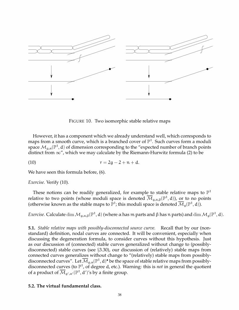
FIGURE 10. Two isomorphic stable relative maps

However, it has a component which we already understand well, which corresponds tomaps from a smooth curve, which is a branched cover of P1. Such curves form a modulispace Mg,α(P1, d) of dimension corresponding to the “expected number of branch pointsdistinct from ∞”, which we may calculate by the Riemann-Hurwitz formula (2) to be

(10) r = 2g− 2+ n+ d.

We have seen this formula before, (6).

Exercise. Verify (10).

These notions can be readily generalized, for example to stable relative maps to P1

relative to two points (whose moduli space is denoted Mg,α,β(P1, d)), or to no points(otherwise known as the stable maps to P1; this moduli space is denoted Mg(P

1, d)).

Exercise. Calculate dimMg,α,β(P1, d) (whereα hasm parts andβ hasn parts) and dimMg(P1, d).

5.1. Stable relative maps with possibly-disconnected source curve. Recall that by our (non-standard) definition, nodal curves are connected. It will be convenient, especially whendiscussing the degeneration formula, to consider curves without this hypothesis. Justas our discussion of (connected) stable curves generalized without change to (possibly-disconnected) stable curves (see §3.30), our discussion of (relatively) stable maps fromconnected curves generalizes without change to “(relatively) stable maps from possibly-disconnected curves”. Let Mg,α(P1, d)• be the space of stable relative maps from possibly-disconnected curves (to P1, of degree d, etc.). Warning: this is not in general the quotientof a product of Mg′,α′(P1, d ′)’s by a finite group.

5.2. The virtual fundamental class.

38

There is a natural homology (or Chow) class on Mg,α(P1, d) of dimension r = dimMg,α(P1, d)

(cf. (10)), called the virtual fundamental class [Mg,α(P1, d)]virt ∈ Ar(Mg,α(P1, d)]), which isobtained from the deformation-obstruction theory of stable relative maps, and has manywonderful properties. The virtual fundamental class agrees with the actual fundamentalclass on the open subset Mg,α(P1, d). The most difficult part of dealing with the modulispace of stable relative maps is working with the virtual fundamental class.

Aside: relative Gromov-Witten invariants. In analogy with usual Gromov-Witten invari-ants, one can define relative Gromov-Witten invariants by intersecting natural cohomologyclasses on the moduli space with the virtual fundamental class. More precisely, one mul-tiplies (via the cup/cap product) the cohomology classes with the virtual fundamentalclass, and takes the degree of the resulting zero-cycle. One can define ψ-classes and λ-classes in the same way as before, and include these in the product. When includingψ-classes, the numbers are often called descendant relative invariants; when including λ-classes, the numbers are sometimes called Hodge integrals for some reason. For example,one can show that Hurwitz numbers are descendant relative invariants of P1. However,this point of view turns out to be less helpful, and we will not use the language of relativeGromov-Witten invariants again.

The virtual fundamental class behaves well under two procedures: degeneration andlocalization; we now discuss these.

5.3. The degeneration formula for the virtual fundamental class, following [Li2].

We describe the degeneration formula in the case of stable maps to P1 relative to onepoint, and leave the cases of stable maps to P1 relative to zero or two points as straightfor-ward variations for the reader. In this discussion, we will deal with possibly-disconnectedcurves to simplify the exposition.

Consider the maps to P1 relative to one point ∞, and imagine deforming the target sothat it breaks into two P1’s, meeting at a node (with ∞ on one of the components). Itturns out that the virtual fundamental class behaves well under this degeneration. Thelimit can be expressed in terms of virtual fundamental classes of spaces of stable relativemaps to each component, relative to ∞ (for the component containing ∞), and relative tothe node-branch (for both components).

Before we make this precise, we give some intuition. Suppose we have a branchedcoverC → P1, and we deform the target into a union of two P1’s, while keeping the branchpoints away from the node; call the limit map C ′ → P1 ∪ P1. Clearly in the limit, awayfrom the node, the cover looks just the same as it did before (with the same branching).At the node, it turns out that the branched covers of the two components must satisfy thekissing/predeformability condition. Say that the branching above the node correspondsto the partition γ1 + · · · + γm. By our discussion about Hurwitz numbers, as we havespecified the branch points, there will be a finite number of such branched covers — wecount branched covers of each component of P1 ∪ P1, with branching corresponding tothe partition γ above the node-branch; then we choose how to match the preimages ofthe node-branch on the two components (there are # Autγ such choices). It turns out

39

that γ1 · · ·γm covers of the original sort will degenerate to each branched cover of thenodal curve of this sort. (Notice that if we were interested in connected curves C, thenthe inverse image of each component of P1 would not necessarily be connected, and wewould have to take some care in gluing these curves together to get a connected union.This is the reason for considering possibly-disconnected components.)

Motivated by the previous paragraph, we give the degeneration formula. Consider the

degeneration of the target (P1,∞) ///o/o/o P1 ∪ (P1,∞) . Let (X,∞) be the general target,

and let (X ′,∞) be the degenerated target. Let (X1, a1) ∼= (P1,∞) denote the first com-ponent of X ′, where a1 refers to the node-branch, and let (X2, a2,∞) ∼= (P1, 0,∞) denotethe second component of X ′, where a2 corresponds to the node branch. Then for eachpartition γ1 + · · ·+ γm = d, there is a natural map

(11) Mg1,γ(P1, d)• ×Mg2,γ,α(P1, d)• → Mg1+g2−m+1,α(X ′, d)•

obtained by gluing the points above a1 to the corresponding points above a2. The imageof this map can be suitably interpreted as stable maps to X ′, satisfying the kissing condi-tion, which can appear as the limit of maps to X. (We are obscuring a delicate issue here— we have not defined stable maps to a singular target such as X.) Then Li’s degenerationformula states that the image of the product of the virtual fundamental classes in (11) isthe limit of the virtual fundamental class of Mg,α(P1, d)•, multiplied by γ1 · · ·γm.

The main idea behind Li’s proof is remarkably elegant, but as with any argument in-volving the virtual fundamental class, the details are quite technical.

If we are interested in connected curves, then there is a corresponding statement (thatrequires no additional proof): we look at the component of the moduli space on the rightside of (11) corresponding to maps from connected source curves, and we look at justthose components of the moduli spaces on the left side which glue together to give con-nected curves.

5.4. Relative virtual localization [GrV3].

The second fundamental method of manipulating virtual fundamental classes is bymeans of localization. Before discussing localization in our Gromov-Witten-theoretic con-text, we first quickly review localization in its original setting.

(A friendly introduction to equivariant cohomology is given in [HKKPTVVZ, Ch. 4],and to localization on the space of ordinary stable maps in [HKKPTVVZ, Ch. 27].)

Suppose Y is a complex projective manifold with an action by a torus C∗. Then thefixed point loci of the torus is the union of smooth submanifolds, possibly of variousdimensions. Let the components of the fixed locus be Y1, Y2, . . . . The torus acts on thenormal bundle Ni to Yi. Then the Atiyah-Bott localization formula states that

(12) [Y] =∑

fixed

[Yi]/ctop(Ni) =∑

fixed

[Yi]/e(Ni),

in the equivariant homology of Y (with appropriate terms inverted), where ctop (or the Eulerclass e) of a vector bundle denotes the top Chern class. This is a wonderfully powerful

40

fact, and to appreciate it, you must do examples yourself. The original paper of Atiyahand Bott [AB] is beautifully written and remains a canonical source.

You can cap (12) with various cohomology classes to get 0-dimensional classes, andget an equality of numbers. But you can cap (12) with classes to get higher-dimensionalclasses, and get equality in cohomology (or the Chow ring). One lesson I want to empha-size is that this is a powerful thing to do. For example, in a virtual setting, in Gromov-Witten theory, localization is traditionally used to get equalities of numbers. We will alsouse equalities of numbers to prove the ELSV formula (8). However, using more generallyequalities of classes will give us Theorem ?, and part of Faber’s conjecture.

Localization was introduced to Gromov-Witten theory by Kontsevich in his ground-breaking paper [Ko2], in which he works on the space of genus zero maps to projectivespace, where the virtual fundamental class is the usual fundamental class (and hencethere are no “virtual” technicalities). In the foundational paper [GrP], Graber and Pand-haripande showed that the localization formula (12) works “virtually” on the modulispace of stable maps, where fundamental classes are replaced by virtual fundamentalclasses, and normal bundles are replaced by “virtual normal bundles”. They defined thevirtual fundamental class of a fixed locus, and the virtual normal bundle, and developedthe machinery to deal with such questions.

There is one pedantic point that must be made here. The localization formula shouldreasonably be expected to work in great generality. However, we currently know it onlysubject to certain technical hypotheses. (1) The proof only works in the algebraic category.(2) In order to apply this machinery, the moduli space must admit a C∗-equivariant locallyclosed immersion into an orbifold. (3) The virtual fundamental class of this fixed locusneeds to be shown to arise from the C∗-fixed part of the obstruction theory of the modulispace. It would be very interesting, and potentially important, to remove hypotheses (1)and (2).

The theory of virtual localization can be applied to our relative setting [GrV3]. (See[LLZ] for more discussion.) We now describe it in the case of interest to us, of maps to P1.Again, in order to understand this properly, you should work out examples yourself.

Fix a torus action on P1

σ [x;y] = [σx;y],

so the torus acts with weight 1 on the tangent space at 0 and −1 on the tangent space at∞. (The weight is the one-dimensional representation, or equivalently, the character.) Thistorus action induces an obvious torus action on Mg,α(P1, d)• (and Mg,α(P1, d)).

We first determine the torus-fixed points of this action. Suppose C → T → X is such afixed map. A picture of two fixed maps showing “typical” behavior is given in Figure 11.The first has “nothing happening above ∞X”, and the second has some “sprouting” ofTi’s.

The map C → Xmust necessarily be a covering space away from the points 0 and ∞ ofX = P1.

41

f−1(∞X) = f−11

(∞T )

0 ∞T

0 ∞X

(a)

(b)

(c)

f−1(0)

C

T

X

0

0 ∞X

(a)

(b)

(c)

f−1(0)

C

T

X

∞T

f−11

(∞T )

(d)

FIGURE 11. Two examples of torus-fixed stable relative maps to (P1,∞)

Exercise. Using the Riemann-Hurwitz formula, show that a surjective map C ′ → P1 froman irreducible curve, unbranched way from 0 and ∞ must be of the form P1 → P1, [x;y] 7→[xa;ya] for some a.

5.5. Hence the components dominating Xmust be a union of “trivial covers” of this sort.

We now focus our attention on the preimage of 0. Any sort of (stable) behavior above 0is allowed. For example, the curve could be smooth and branched there (Figure 11(a)); ortwo of the trivial covers could meet in a node (Figure 11(b)); or there could be a contractedcomponent of C, intersecting various trivial components at nodes (Figure 11(c)). (Becausethe “relative” part of the picture is at ∞, this discussion is the same as the discussion forordinary stable maps, as discussed in [GrP].)

Finally, we consider the preimage of ∞X. Possibly “nothing happens over ∞”, i.e. thetarget has not sprouted a tree (l = 0 in our definition of stable relative maps at the startof §5), and the preimage of ∞ consists just of n smooth points; this is the first example inFigure 11. Otherwise, there is some “sprouting” of the target, and something “nontrivial”happens above each sprouted component Ti (i > 0), as in Figure 11(d).

5.6. At this point, you should draw some pictures, and convince yourself of the followingimportant fact: the connected components of the fixed locus correspond to certain discretedata. In particular, each connected component can be interpreted as a product of threesorts of moduli spaces:

42

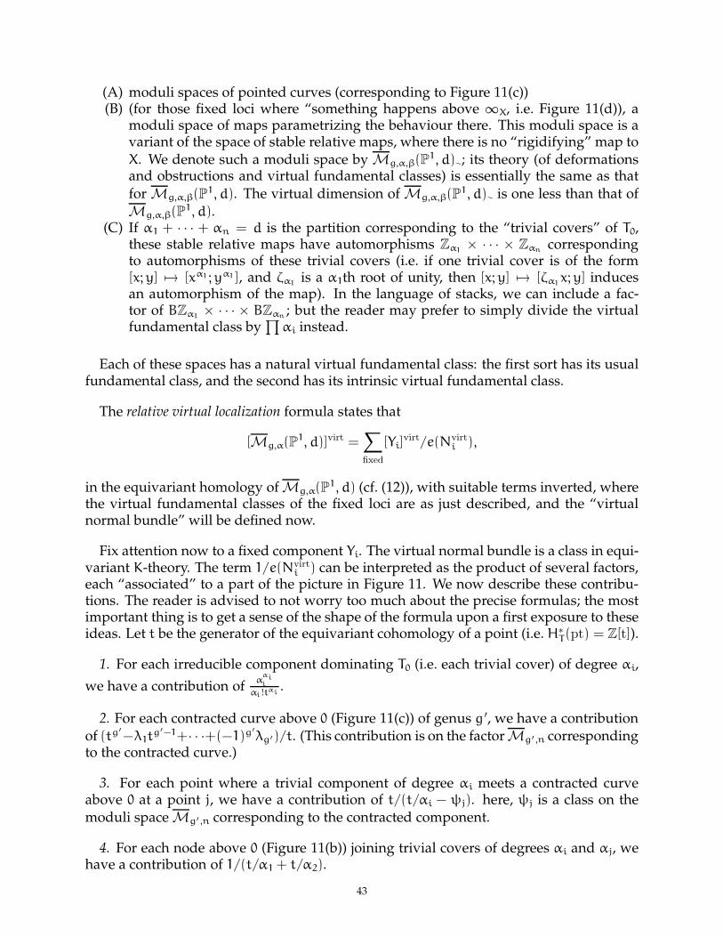
(A) moduli spaces of pointed curves (corresponding to Figure 11(c))(B) (for those fixed loci where “something happens above ∞X, i.e. Figure 11(d)), a

moduli space of maps parametrizing the behaviour there. This moduli space is avariant of the space of stable relative maps, where there is no “rigidifying” map toX. We denote such a moduli space by Mg,α,β(P1, d)∼; its theory (of deformationsand obstructions and virtual fundamental classes) is essentially the same as thatfor Mg,α,β(P1, d). The virtual dimension of Mg,α,β(P1, d)∼ is one less than that ofMg,α,β(P1, d).

(C) If α1 + · · · + αn = d is the partition corresponding to the “trivial covers” of T0,these stable relative maps have automorphisms Zα1

× · · · × Zαn correspondingto automorphisms of these trivial covers (i.e. if one trivial cover is of the form[x;y] 7→ [xα1 ;yα1 ], and ζα1

is a α1th root of unity, then [x;y] 7→ [ζα1x;y] induces

an automorphism of the map). In the language of stacks, we can include a fac-tor of BZα1

× · · · × BZαn ; but the reader may prefer to simply divide the virtualfundamental class by

∏αi instead.

Each of these spaces has a natural virtual fundamental class: the first sort has its usualfundamental class, and the second has its intrinsic virtual fundamental class.

The relative virtual localization formula states that

[Mg,α(P1, d)]virt =∑

fixed

[Yi]virt/e(Nvirt

i ),

in the equivariant homology of Mg,α(P1, d) (cf. (12)), with suitable terms inverted, wherethe virtual fundamental classes of the fixed loci are as just described, and the “virtualnormal bundle” will be defined now.

Fix attention now to a fixed component Yi. The virtual normal bundle is a class in equi-variant K-theory. The term 1/e(Nvirt

i ) can be interpreted as the product of several factors,each “associated” to a part of the picture in Figure 11. We now describe these contribu-tions. The reader is advised to not worry too much about the precise formulas; the mostimportant thing is to get a sense of the shape of the formula upon a first exposure to theseideas. Let t be the generator of the equivariant cohomology of a point (i.e.H∗

T(pt) = Z[t]).

1. For each irreducible component dominating T0 (i.e. each trivial cover) of degree αi,

we have a contribution ofα

αii

αi!tαi

.

2. For each contracted curve above 0 (Figure 11(c)) of genus g ′, we have a contributionof (tg

′

−λ1tg′−1+· · ·+(−1)g′

λg′)/t. (This contribution is on the factor Mg′,n correspondingto the contracted curve.)

3. For each point where a trivial component of degree αi meets a contracted curveabove 0 at a point j, we have a contribution of t/(t/αi − ψj). here, ψj is a class on themoduli space Mg′,n corresponding to the contracted component.

4. For each node above 0 (Figure 11(b)) joining trivial covers of degrees αi and αj, wehave a contribution of 1/(t/α1 + t/α2).

43

5. For each smooth point above 0 (Figure 11(a)) on a trivial cover of degree αi, we havea contribution of t/αi.

At this point, if you squint and ignore the t’s, you can almost see the ELSV formula (8)taking shape.

6. If there is a component over ∞X, then we have a contribution of 1/(−t − ψ), whereψ is the first Chern class of the line bundle corresponding to the cotangent space of T1 atthe point where it meets T0.

These six contributions look (and are!) complicated. But this formula can be judiciouslyused to give some powerful results, surprisingly cheaply. We now describe some of these.

6. APPLICATIONS OF RELATIVE VIRTUAL LOCALIZATION

6.1. Example 1: proof of the ELSV formula (8).

As a first example, we prove the ELSV formula (8). (This formula follows [GrV1], usingthe simplification in the last section of [GrV1] provided by the existence of Jun Li’s de-scription of the moduli space of stable relative maps.) The ELSV formula counts branchedcovers with specified branching over ∞ corresponding to α ` d, and other fixed simplebranched points. Hence we will consider Mg,α(P1, d).

We next need to impose other fixed branch points. There is a natural Gromov-Witten-theoretic approach involving using descendant invariants, but this turns out to be thewrong thing to do. Instead, we use a beautiful construction of Fantechi and Pandhari-pande [FanP]. Given any map from a nodal curve to P1, we can define a branch divisor onthe target. When the source curve is smooth, the definition is natural (and old): above apoint p corresponding to a partition β ` d, the branch divisor contains pwith multiplicity∑

(βi − 1). It is not hard to figure out how extend this to the case where the source curveis not smooth above p.

Exercise. Figure out what this extension should be. (Do this so that the Riemann-Hurwitzformula remains true.)

Thus we have a map of sets Mg(P1, d) → Sym2d+2g−2 P1. In the case of stable relative

maps, we have a map of sets Mg,α(P1, d) → Sym2d+2g−2 P1. As each such stable relativemap will have branching of at least

∑(αi − 1) above ∞, we can subtract this fixed branch

divisor to get a map of sets

(13) br : Mg,α(P1, d) → Symr P1

where r = 2d+ 2g− 2−∑

(αi − 1) = 2g− 2+ d + n (cf. (10)).

The important technical result proved by Fantechi and Pandharipande is the following.

6.2. Theorem (Fantechi-Pandharipande [FanP]). — There is a natural map of stacks br as in (13).

44

We call such a map a (Fantechi-Pandharipande) branch morphism. This morphism respectsthe torus action.

One can now readily verify several facts. If the branch divisor does not contain p 6= ∞in P1, then the corresponding map C → P1 is unbranched (i.e. a covering space, or etale)above p. If the branch divisor contains p 6= ∞ with multiplicity 1, then the correspondingmap is simply branched above p. (Recall that this means that the preimage of p consistsof smooth points, and the branching corresponds to the partition 2 + 1 + · · · + 1.) If thebranch divisor does not contain ∞, i.e. there is no additional branching above ∞X beyondthat required by the definition of stable relative map, then the preimage of ∞X consistsprecisely of the n smooth points qi. In other words, there is no “sprouting” of Ti, i.e. T ∼=

P1. Hence if p1+· · ·+pr is a general point of Symr P1, then br−1(p1+· · ·+pr) ⊂ Mg,α(P1, d)

is a finite set of cardinality equal to the Hurwitz number Hgα. This is true despite the fact

that Mg,α(P1, d) is horribly non-equidimensional — the preimage of a general point ofSymr P1 will be contained in Mg,α(P1, d), and will not meet any other nasty components!

By turning this set-theoretic argument into something more stack-theoretic and precise,we have that

(14) Hgα = deg br−1(pt) ∩ [Mg,α(P1, d)]virt.

(For distracting unimportant reasons, the previous paragraph’s discussion is slightly in-correct in the case where Hg

α = 1/2, but (14) is true.)

We can now calculate the right side of (14) using localization. In order to do this, weneed to interpret it equivariantly, which involves choosing an equivariant lift of br−1 of apoint in Symr P1 ∼= Pr. We do this by choosing our point in Symr P1 to be the point 0 withmultiplicity r. Thus all the branching (aside from that forced to be at ∞) must be at 0.The normal bundle to this point of Pr is r!tr. Thus when we apply localization, a miraclehappens. The only fixed loci we consider are those where there is no extra branchingover ∞ (see the first picture in Figure 11). However, the source curve is smooth, so thereis in fact only one connected component of the fixed locus to consider, which is shown inFigure 12. The moduli space in this case is Mg,n, which we take with multiplicity 1/

∏αi

(cf. §5.6(C)). Hence the Hurwitz number is the intersection on this moduli space of thecontributions to the virtual normal bundle outlined above.

Exercise. Verify that the contributions from 1, 2, and 3 above, on the moduli space Mg,n,give the ELSV formula (8).

6.3. Example 2: Proof of Theorem ? (Theorem 4.1).

In Example 1 (§6.1), we found an equality of numbers. Here we will use relative virtuallocalization to get equality of cohomology or Chow classes.

Fix g and n. We are interested in dimension j (tautological) classes on Mg,n. In particu-lar, we wish to show that any such tautological class can be deformed into one supportedon the locus corresponding to curves with at least 2g − 2 + n − j genus 0 components.(This is just a restatement of Theorem ?.) Call such a dimension j class good. Using the

45

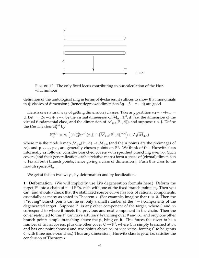
∞0

T = X

FIGURE 12. The only fixed locus contributing to our calculation of the Hur-witz number

definition of the tautological ring in terms ofψ-classes, it suffices to show that monomialsin ψ-classes of dimension j (hence degree=codimension 3g− 3+ n − j) are good.

Here is one natural way of getting dimension j classes. Take any partition α1+· · ·+αn =

d. Let r = 2g−2+n+d be the virtual dimension of Mg,α(P1, d) (i.e. the dimension of thevirtual fundamental class, and the dimension of Mg,α(P1, d)), and suppose r > j. Definethe Hurwitz class H

g,αj by

Hg,αj := π∗

(

(∩r−ji=1br

−1(pi)) ∩ [Mg,α(P1, d)]virt)

∈ Aj(Mg,n)

where π is the moduli map Mg,α(P1, d) → Mg,n (and the n points are the preimages of∞), and p1, . . . , pr−j are generally chosen points on P1. We think of this Hurwitz classinformally as follows: consider branched covers with specified branching over ∞. Suchcovers (and their generalization, stable relative maps) form a space of (virtual) dimensionr. Fix all but j branch points, hence giving a class of dimension j. Push this class to themoduli space Mg,n.

We get at this in two ways, by deformation and by localization.

1. Deformation. (We will implicitly use Li’s degeneration formula here.) Deform thetarget P1 into a chain of r − j P1’s, each with one of the fixed branch points pi. Then youcan (and should) check that the stabilized source curve has lots of rational components,essentially as many as stated in Theorem ?. (For example, imagine that r 0. Then thej “roving” branch points can lie on only a small number of the r − j components of thedegenerated target. Suppose P1 is any other component of the target, where 0 and ∞correspond to where it meets the previous and next component in the chain. Then thecover restricted to this P1 can have arbitrary branching over 0 and ∞, and only one otherbranch point: simple branching above the pi lying on it. This forces the cover to be anumber of trivial covers, plus one other cover C → P1, where C is simply branched at pi,and has one point above 0 and two points above ∞, or vice versa, forcing C to be genus0, with three node-branches.) Thus any dimension jHurwitz class is good, i.e. satisfies theconclusion of Theorem ?.

46

2. Localization. We next use localization to express tautological classes in terms of Hur-witz classes. In the same way as for the ELSV formula, we choose an equivariant lifting

of ∩r−ji=1br

−1(pi), corresponding to requiring all the pi to go to 0. (Unlike the ELSV case,there are still j branch points that could go to either 0 or ∞.)

We now consider what fixed components can arise.

We have one “main” component that is similar to the ELSV case, where all the j “rov-ing” branch points go to 0 (Figure 12). Any other component will be nontrivial over ∞.One can readily inductively show that these other components are good, i.e. satisfy theconclusion of Theorem ?. (The argument is by looking at the contribution from such afixed locus. The part contained in f−1(∞X) is essentially a Hurwitz class, which we haveshown is good. The part contained in f−1(0) corresponds to tautological classes on modulispaces of curves with smaller 2g− 2+ n, which can be inductively assumed to be good.)

Thus we have shown that the contribution of the “main” component is good. But thiscontribution is straightforward to contribute: it is (up to multiple) the dimension j com-ponent of

1− λ1 + · · · + (−1)gλg

(1− α1ψ1) · · · (1− αnψn)

(compare this to the ELSV formula (8)). By expanding this out, we find a polynomial inthe αi of degree 3g − 3 + n − j (cf. (9) for a similar argument earlier). We then apply thesame trick as when we computed top intersections ofψ-classes using Hurwitz numbers in§3.20: we can recover the co-efficients in this polynomial by “plugging in enough values”.In other words, ψa1

1 · · ·ψa1n may be obtained (modulo good classes) as a linear combination

of Hurwitz classes. As Hurwitz classes are themselves good, we have shown that themonomial ψa1

1 · · ·ψa1n is also good, completing the argument.

7. TOWARDS FABER’S INTERSECTION NUMBER CONJECTURE 3.23 VIA RELATIVE

VIRTUAL LOCALIZATION

We can use the methods of the proof of Theorem ? to combinatorially describe the topintersections in the tautological ring. Using this, one can prove the “vanishing” or “socle”portion of the Faber-type conjecture for curves with rational tails (and hence for Mg), andprove Faber’s intersection number conjecture for up to three points. Details will be givenin [GJV3]; here we will just discuss the geometry involved.

The idea is as follows. We are interested in the Chow ring of Mrtg,n, so we will work on

compact moduli spaces, but discard any classes that vanish on the locus of curves withrational tails. We make a series of short geometric remarks.

First, note that R2g−1(Mrtg,n) → R2g−1(Mg,1) is an isomorphism, and R2g−1(Mg,1) →

R2g−1(Mg) is a surjection. The latter is immediate from our definition. The argument forthe former is for example [GrV3, Prop. 5.8], and can be taken as an exercise for the readerusing Theorem ?. Faber showed [Fab1, Thm. 2] that R2g−1(Mg) is non-trivial, so if we canshow that R2g−1(Mg,1) is generated by a single element, then we will have proved thatR2g−1(M

rtg,n) ∼= Q for all n ≥ 0.

47

7.1. An extension of that argument using Theorem ? shows that if we have a Hurwitzclass of dimension less than 2g− 1 (i.e. with fewer than 2g− 1 “moving branch points”),then the class is 0 in A∗(M

rtg,n).

In order to get a hold of R2g−1(Mrtg,n), we will again use branched covers. Before getting

into the Gromov-Witten theory, we make a series of remarks, that may be verified by thereader, using only the Riemann-Hurwitz formula (2).

7.2. First, suppose we have a map C → P1 from a nodal (possibly disconnected) curve,unbranched away from 0 and ∞. Then it is a union of a trivial covers (in the sense of §5.5).

7.3. Second, suppose we have a map from a nodal curve C to P1, with no branchingaway from 0 and ∞ except for simple branching over 1, and nonsingular over 0 and ∞.Then it is a union of trivial covers, plus one more component, that is genus 0, completelybranched over one of 0,∞, and with two preimages over the other. More generally, sup-pose we have a map from some curve C to a chain of P1’s, satisfying the kissing condition,unbranched except for two smooth points 0 and ∞ on the ends of the chain, and simplebranching over another point 1. Then the map is the union of a number of trivial coversglued together, plus one other cover P1 → P1 of the component containing 1, of the sortdescribed in the previous sentence.

7.4. Third, if we have a map from a nodal curve C to P1, with total branching away from0 and ∞ of degree less than 2g, and nonsingular over 0 and ∞, then C has no componentof geometric genus g. In the same situation, if the total branching away from 0 and ∞is exactly g, and C has a component of geometric genus g, then the cover is a disjointunion of trivial covers, and one connected curve C ′ of arithmetic genus g, where the mapC ′ → P1 is contracted to 1 or completely branched over 0 and ∞.

More generally, if we have a map from a curve C to a chain of P1’s satisfying the kissingcondition, with 0 and ∞ points on either ends of the chain, with total branching away lessthan 2g away from 0, ∞, and the nodes, then C has no component of geometric genus g.In the same situation, if the total branching away from 0, ∞, and the nodes is precisely2g, then the map is the union of a number of trivial covers glued together, plus one othercover of the sort described in the previous paragraph.

7.5. The following fact is trickier. Let Zg,d be the image in A2g−1(Mg,1) of br−1(1) ∩

[Mg,(d),(d)(P1, d)]virt (where the point in Mg,1 is the preimage of ∞). Then Zg,d = d2gZg,1.

(We omit the proof, but the main idea behind this is the Fourier-Mukai fact [Lo, Lemma 2.10].)

Define the Faber-Hurwitz class Fg,α as the image in A2g−1(Mrt

g,n) of

∩r−(2g−1)

i=1 br−1(pi) ∩ [Mg,1(P1, d)]virt

where the pi are general points of P1. (This is the image of a Hurwitz class in Mrt

g,n.)

48

As with the proof of Theorem ?, we get at this class inductively using degeneration,and connect it to intersections of ψ-classes using localization.

7.6. Degeneration.

Break the target into two pieces P1 ///o/o/o P1 ∪ P1 , where ∞ and one pi are on the “right”

piece, and the remaining pi’s are on the “left” piece. The Faber-Hurwitz class breaks intovarious pieces; we enumerate the possibilities. We are interested only in componentswhere there is a nonsingular genus g curve on one side. We have two cases, dependingon whether this curve maps to the “left” or the “right” P1.

7.7. If it maps to the left component, then all 2g−1 “moving” branch points must also mapto the left component in order to get a non-zero contribution in A∗(M

rtg,n), by Remark 7.4.

Thus by Remark 7.3, the cover on the right is of a particular sort, and the cover on the leftis another Faber-Hurwitz class, where one of the branch points over ∞ has been replacedtwo, or where two of the branch points are replaced by one.

7.8. If the genus g curve maps to the right component, then all 2g − 1 “moving” branchpoints must map to the right component, and by Remark 7.4 our contribution is a certainmultiple of Zg,d, which by Remark 7.5 is a certain multiple of Zg,1. The contribution fromthe left is the genus 0 Hurwitz number H0

α, for which Hurwitz gives us an attractiveformula (7).

Unwinding this gives the recursion

(15) Fgα =

∑

i+j=αk

ijH0α′F

gα′′

(

d+ l(α) − 2

d+ l(α ′) − 2, d+ l(α ′′) − 1

)

+∑

αi+αj

Fgα′ +

l(α)∑

i=1

α2g+1i H0

αZg,1.

In this formula, the contributions from paragraph §7.8 are in the first two terms on theright side of the equation, and the contributions from §7.7 are in the last. The second termon the right corresponds to where two parts αi and αj of α are “joined” by the nontrivialcover of the right P1 to yield a new partition where αi and αj are replaced by αi + αj.The first term on the right corresponds to where one part αk of α is “cut” into two piecesi and j, forcing the curve covering the left P1 to break into two pieces, one of genus 0(corresponding to partition α ′ and one of genus g (corresponding to α ′). The binomialcoefficient corresponds to the fact that the d + l(α) − 2 fixed branch points p1, p2, . . . onthe left component must be split between these two covers.

The base case is Fg

(1)= Zg,1. Hence we have shown that Fg

α is always a multiple of

Zg,1, and the theory of cut-and-join type equations (developed notably by Goulden andJackson) can be applied to solve for Fg

α (in generating function form) quite explicitly.

7.9. Localization.

We now get at the Faber-Hurwitz class by localizing. As with the proof of Theorem ?,we choose a linearization on br−1(pi) that corresponds to requiring all the pi to move

49

to 0. We now describe the fixed loci that contribute. We won’t worry about the precisecontribution of each fixed locus; the important thing is to see the shape of the formula.

First note that as we have only 2g − 1 moving branch points, in any fixed locus in the“rational-tails” locus, our genus g component cannot map to ∞, and thus must be con-tracted to 0. The fixed locus can certainly have genus 0 components mapping to sproutedTi over ∞, as well as genus 0 components contracted to 0.

We now look at the contribution of this fixed locus, via the relative virtual localizationformula. We will get a sum of classes glued together from various moduli spaces ap-pearing in the description of the fixed locus (cf. §5.6). Say the contracted genus g curvemeetsm trivial covers, of degree β1, . . . , βm respectively. Then the contribution from thiscomponent will be some summand of

1− λ1 + · · · + (−1)gλg

(1− β1ψ1) · · · (1− βmψm)

whereψi are theψ-classes on Mg,m. Thus the contribution from this component is visiblytautological, and by Remark 7.1 the contribution will be zero if the dimension of the classis less than 2g − 1. As the total contribution of this fixed locus is 2g − 1, any non-zerocontribution must correspond to a dimension 2g− 1 tautological class on Mg,m glued toa dimension 0 class on the other moduli spaces appearing in this fixed locus. This canbe readily computed; the genus 0 components contracted to 0 yield binomial coefficients,any components over ∞X turn out to yield products of genus 0 double Hurwitz numbers,which count branched covers of P1 by a genus 0 curve, with specified branching α and βabove two points, and the remaining branching fixed and simple.

Equipped with this localization formula, even without worrying about the specificcombinatorics, we may show the following.

7.10. Theorem. — For any n, and β ` d, π∗ψβ1

1 · · ·ψβnn is a multiple of Zd,1, where π is the

forgetful map to Mg,1.

We have thus fully shown the “vanishing” (or socle) part of Faber’s conjecture forcurves with rational tails. (This may certainly be shown by other means.) In particular,we have completed a proof of Looijenga’s Theorem 4.5.

Proof. Call such a class an n-point class. We will show that such a class is a multiple ofZd,1 modulom-point classes, wherem < n; the result then follows by induction. As withthe proof of Theorem ?, we consider Fα

g as α runs over all partitions of length n. Eachsuch Faber-Hurwitz class is a multiple of Zd,1 by our degeneration analysis. By our local-ization analysis, all of the fixed points for Fα

g yield m-point classes where m < n exceptfor one, corresponding to the picture in Figure 12. The contribution of this component issome known multiple of a polynomial in α1, . . . , αn. The highest-degree coefficients ofthis polynomial are the n-point classes, the monomials in ψ-classes that we seek. By tak-ing a suitable linear combination of values of the polynomial (i.e. Faber-Hurwitz classes,modulo m-point classes where m < n), we can obtain any co-efficient, and in particular,the leading co-efficients.

50

A related observation is that we have now given an explicit combinatorial descriptionof the monomials in ψ-classes, as a multiple of our generator Zg,1. (In truth, we have notbeen careful in this exposition in describing all the combinatorial factors. See [GJV3] fora precise description.)

This combinatorialization can be made precise as follows. We create a generating func-tion F for Faber-Hurwitz classes. The join-cut equation (15) allows us to solve for thegenerating function F.

We make a second generating function W for the intersections π∗ψβ1

1 · · ·ψβnn λk ∈ R2g−1(Mg,1)

(where β1 + · · · + βn + k = g − 2). Localization gives us a description of F in terms of W

(and also the genus 0 double Hurwitz generating function). By inverting this relationshipwe can hope to solve relatively explicitly for W, and hence prove Faber’s intersectionnumber conjecture. Because genus 0 double Hurwitz number H0

α,β are only currentlywell-understood when one of the partition has at most 3 parts (see [GJV2]), this programis not yet complete. However, it indeed yields:

7.11. Theorem [GJV3]. — Faber’s intersection number conjecture is true for up to three points.

One might reasonably hope that this will give an elegant proof of Faber’s intersectionnumber conjecture in full before long.

8. CONCLUSION

In the last fifteen years, there has been a surge of progress in understanding curves andtheir moduli using the techniques of Gromov-Witten theory. Many of these techniqueshave been outlined here.

Although this recent progress uses very modern machinery, it is part of an ancient story.Since the time of Riemann, algebraic curves have been studied by way of branched cov-ers of P1. The techniques described here involve thinking about curves in the same way.Gromov-Witten theory gives the added insight that we should work with a “compacti-fication” of the space of branched covers, the moduli space of stable (relative) maps. Apriori we pay a steep price, by working with a moduli space that is bad in all possibleways (singular, reducible, not even equidimensional). But it is in some sense “virtuallysmooth”, and its virtual fundamental class behaves very well, in particular with respectto degeneration and localization.

The approaches outlined here have one thing in common: in each case the key ideais direct and naive. Then one works to develop the necessary Gromov-Witten-theoretictools to make the naive idea precise.

In conclusion, the story of using Gromov-Witten theory to understand curves, and tounderstand curves by examining how they map into other spaces (such as P1), is mostcertainly not over, and may just be beginning.

51

REFERENCES

[ArbC] E. Arbarello and M. Cornalba, The Picard groups of the moduli spaces of curves, Topology 26(1987), 153–171.

[ArcL1] D. Arcara and Y.-P. Lee, Tautological equations in genus 2 via invariance conjectures, preprint2005, math.AG/0502488.

[ArcL2] D. Arcara and Y.-P. Lee, Tautological equations in M3,1 via invariance conjectures, preprint2005, math.AG/0503184.

[Arn] V. I. Arnol’d, Topological classification of trigonometric polynomials and combinatorics of graphswith an equal number of vertices and edges, Funct. Anal. and its Appl. 30 no. 1 (1996), 1–17.

[AB] M. Atiyah and R. Bott, The moment map and equivariant cohomology, Topology 23 (1984),1–28.

[BP] P. Belorousski and R. Pandharipande, A descendent relation in genus 2, Ann. Scuola Norm.Sup. Pisa Cl. Sci. (4) 29 (2000), no. 1, 171–191.

[C] K. Costello, Higher-genus Gromov-Witten invariants as genus 0 invariants of symmetric prod-ucts, preprint 2003, math.AG/0303387.

[CK] D. Cox and S. Katz, Mirror Symmetry and Algebraic Geometry, Mathematical surveys andMonographs 68, Amer. Math. Soc., Providence, RI, 1999.

[CT] M. Crescimanno and W. Taylor, Large N phases of chiral QCD2, Nuclear Phys. B 437 (1995),3–24.

[D] J. Denes, The representation of a permutation as the product of a minimal number of transpositionsand its connection with the theory of graphs, Publ. Math. Ins. Hungar. Acad. Sci. 4 (1959), 63–70.

[DVV] R. Dijkgraaf, H. Verlinde, and E. Verlinde, Topological strings in d < 1, Nuclear Phys. B 352(1991), 59–86.

[E] D. Edidin, Notes on the construction of the moduli space of curves, in Recent progress in inter-section theory (Bologna, 1997), 85–113, Trends Math., Birkhauser Boston, Boston, MA, 2000.MR 1849292

[ELSV1] T. Ekedahl, S. Lando, M. Shapiro, and A. Vainshtein, On Hurwitz numbers and Hodge inte-grals, C. R. Acad. Sci. Paris Ser. I Math. 328 (1999), 1175–1180. MR 1701381

[ELSV2] T. Ekedahl, S. Lando, M. Shapiro, and A. Vainshtein, Hurwitz numbers and intersections onmoduli spaces of curves, Invent. Math. 146 (2001), 297–327. MR 1864018

[Fab1] C. Faber, A conjectural description of the tautological ring of the moduli space of curves, in Moduliof Curves and Abelian Varieties, 109–129, Aspects Math., E33, Vieweg, Braunschweig, 1999.MR1722541

[Fab2] C. Faber, MAPLE program for computing Hodge integrals, personal communication.Available at http://math.stanford.edu/~vakil/programs/.

[Fab3] C. Faber, Algorithms for computing intersection numbers on moduli spaces of curves, with anapplication to the class of the locus of Jacobians, in New trends in algebraic geometry (Warwick,1996), 93–109, London Math. Soc. Lecture Note Ser., 264, Cambridge Univ. Press, Cam-bridge, 1999. MR 1714822

[Fab4] C. Faber, personal communication, January 8, 2006.[FabP1] C. Faber and R. Pandharipande, Logarithmic series and Hodge integrals in the tautological ring,

Michigan Math. J. (Fulton volume) 48 (2000), 215–252. MR 1786488[FabP2] C. Faber and R. Pandharipande, Hodge integrals, partition matrices, and the λg conjecture,

Ann. Math. 157 (2003), 97–124. MR 1954265[FabP3] C. Faber and R. Pandharipande, Relative maps and tautological classes, J. Eur. Math. Soc. 7

(2005), no. 1, 13–49. MR 2120989[Fan] B. Fantechi, Stacks for everybody, in European Congress of Mathematics, Vol. I (Barcelona, 2000),

349–359, Progr. Math., 201, Birkhauser, Basel, 2001.[FanP] B. Fantechi and R. Pandharipande, Stable maps and branch divisors, Compositio Math. 130

(2002), no. 3, 345–364. MR 1887119[Ga] A. Gathmann, Absolute and relative Gromov-Witten invariants of very ample hypersurfaces,

Duke Math. J. 115 (2002), 171–203. MR 1944571

52

[Ge1] E. Getzler, Intersection theory on M1,4 and elliptic Gromov-Witten invariants, J. Amer. Math.Soc. 10 (1997), no. 4, 973–998. MR 1451505

[Ge2] E. Getzler, Topological recursion relations in genus 2, in Integrable systems and algebraic geometry(Kobe/Kyoto, 1997), 73–106, World Sci. Publishing, River Edge, NJ, 1998. MR1672112

[GeP] E. Getzler and R. Pandharipande, Virasoro constraints and the Chern classes of the Hodge bun-dle, Nuclear Phys. B 530 (1998), 701–714.

[GiaM] J. Giansiracusa and D. Maulik, Topology and geometry of the moduli space ofcurves, on-line collection of resources on moduli of curves and related subjects,http://www.aimath.org/WWN/modspacecurves/.

[Giv] A. Givental, Gromov-Witten invariants and quantization of quadratic hamiltonians, Mosc. Math.J. 1 (2001), no. 4, 551–568, 645. MR 1901075

[GJ1] I. P. Goulden and D. M. Jackson, Transitive factorizations into transpositions and holomorphicmappings on the sphere, Proc. Amer. Math. Soc. 125 (1997), 51–60.

[GJ2] I. P. Goulden and D. M. Jackson, The number of ramified coverings of the sphere by the doubletorus, and a general form for higher genera, J. Combin. Theory A 88 (1999) 259–275.

[GJV1] I. P. Goulden, D. M. Jackson, R. Vakil, The Gromov-Witten potential of a point, Hurwitz num-bers, and Hodge integrals, Proc. London Math. Soc. (3) 83 (2001), 563–581.

[GJV2] I. P. Goulden, D. M. Jackson, R. Vakil, Towards the geometry of double Hurwitz numbers, Adv.Math. (Artin issue) 198 (2005), 43–92.

[GJV3] I. P. Goulden, D. M. Jackson, R. Vakil, On Faber’s intersection number conjecture on the modulispace of curves, in preparation.

[GrP] T. Graber and R. Pandharipande, Localization of virtual classes, Invent. Math. 135 (1999),487–518.

[GrV1] T. Graber and R. Vakil, Hodge integrals and Hurwitz numbers via virtual localization, Compo-sitio Math. 135 (2003), no. 1, 25–36. MR 1955162

[GrV2] T. Graber and R. Vakil, On the tautological ring of Mg,n, in Proceedings of the Seventh GokovaGeometry-Topology Conference 2000, International Press, 2000. MR 1829089

[GrV3] T. Graber and R. Vakil, Relative virtual localization and vanishing of tautological classes onmoduli spaces of curves, Duke Math. J. 130 (2005), no. 1, 1–37.

[HLo] R. Hain and E. Looijenga, Mapping class groups and moduli spaces of curves, Proc. Sympos.Pure Math. 62 Part 2, pp. 97–142, Amer. Math. Soc., Providence, RI, 1997. MR 1492535

[HZ] J. Harer and D. Zagier, The Euler characteristic of the moduli space of curves, Invent. Math. 85(1986), no. 3, 457–485.

[HM] J. Harris and I. Morrison, Moduli of Curves, Graduate Texts in Mathematics 187, Springer-Verlag, New York, 1998. MR 1631825

[HKKPTVVZ] K. Hori, S. Katz, A. Klemm, R. Pandharipande, R. Thomas, C. Vafa, R. Vakil, and E. Zaslow,Gromov-Witten Theory and Mirror Symmetry, Clay Math. Inst., Amer. Math. Soc., 2002.

[H] A. Hurwitz, Uber Riemann’sche Flachen mit gegeben Verzweigungspunkten, Math. Ann. 39(1891), 1–60.

[I1] E. Ionel, Topological recursive relations in H2g(Mg,n), Invent. Math. 148 (2002), no. 3, 627–658. MR 1908062

[I2] E. Ionel, Relations in the tautological ring of Mg, Duke Math. J. 129 (2005), no. 1, 157–186.[IP1] E.-N. Ionel and T. H. Parker, Relative Gromov-Witten invariants, Ann. of Math. (2) 157 (2003),

45–96. MR 1954264[IP2] E.-N. Ionel and T. H. Parker, The symplectic sum formula for Gromov-Witten invariants, Ann.

of Math. (2), 159 (2004), 935–1025. MR 2113018[Ke] S. Keel, Intersection theory of moduli space of stable n-pointed curves of genus zero, Trans. Amer.

Math. Soc. 330 (1992), no. 2, 545–574. MR 1034665[KiL] Y.-S. Kim and K. Liu, A simple proof of Witten conjecture through localization, preprint 2005,

math.AG/0508384.[KL] T. Kimura and X. Liu, A genus-3 topological recursion relation, preprint 2005,

math.DG/0502457.[Ko1] M. Kontsevich, Intersection theory on the moduli space of curves and the matrix Airy function,

Comm. Math. Phys. 147 (1992), 1–23.

53

[Ko2] M. Kontsevich, Enumeration of rational curves via torus actions, in the Moduli Space of Curves(Texel Island, 1994), R. Dijkgraaf, C. Faber and G. van der Geer, eds., Progr. Math. vol. 129,Birkhauser, Boston, 1995, pp. 335–368.

[Kr] A. Kresch, Cycle groups for Artin stacks, Invent. Math. 138 (1999), no. 3, 495–536. MR 1719823[Lee1] Y.-P. Lee, Invariance of tautological equations I: Conjectures and applications, preprint 2006.[Lee2] Y.-P. Lee, Invariance of tautological equations II: Gromov-Witten theory, in preparation.[LeeP] Y.-P. Lee and R. Pandharipande, Frobenius manifolds, Gromov-Witten theory, and Virasoro con-

straints, book in preparation.[Li1] J. Li, Stable morphisms to singular schemes and relative stable morphisms, J. Diff. Geom. 57

(2001), 509–578. MR 1882667[Li2] J. Li, A degeneration formula of GW-invariants, J. Diff. Geom. 60 (2002), 199–293. MR 1938113[LR] A.-M. Li and Y. Ruan, Symplectic surgery and Gromov-Witten invariants of Calabi-Yau 3-folds,

Invent. Math. 145 (2001), 151–218. MR 1839289[LLZ] C.-C. M. Liu, K. Liu, and J. Zhou, A proof of a conjecture of Marino-Vafa on Hodge integrals, J.

Diff. Geom. 65 (2004), 289–340.[Lo] E. Looijenga, On the tautological ring of Mg, Invent. Math. 121 (1995), no. 2, 411–419. MR

1346214[MT] I. Madsen and U. Tillmann, The stable mapping class group and Q(CP∞

+ ), Invent. Math. 145(2001), no. 3, 509–544.

[MW] I. Madsen and M. Weiss, The stable moduli space of Riemann surfaces: Mumford’s conjecture,preprint 2002, math.AT/0212321.

[Mi] M. Mirzakhani, Weil-Petersson volumes and the Witten-Kontsevich formula, preprint 2003.[Mo1] S. Morita, Generators for the tautological algebra of the moduli space of curves, Topology 42

(2003), 787–819.[Mo2] S. Morita, Cohomological structure of the mapping class group and beyond, preprint 2005,

math.GT/0507308v1.[Mu] D. Mumford, Toward an enumerative geometry of the moduli space of curves, in Arithmetic and

Geometry, Vol. II, M. Artin and J. Tate ed., 271–328, Prog. Math. 36, Birk. Boston, Boston,MA, 1983. MR 0717614

[OP] A. Okounkov and R. Pandharipande, Gromov-Witten theory, Hurwitz numbers, and matrixmodels, I, math.AG/0101147.

[P] R. Pandharipande, Three questions in Gromov-Witten theory, in Proceedings of the InternationalCongress of Mathematicians, Vol. II (Beijing, 2002), 503–512, Higher Ed. Press, Beijing, 2002.

[R] B. Riemann, Theorie der Abel’schen Funktionen, J. Reine angew. Math. 54 (1857), 115–155.[T] U. Tillmann, Strings and the stable cohomology of mapping class groups, in Proceedings of the

International Congress of Mathematicians, Vol. II (Beijing, 2002), 447–456, Higher Ed. Press,Beijing, 2002.

[V1] R. Vakil, Genus 0 and 1 Hurwitz numbers: Recursions, formulas, and graph-theoretic interpreta-tions, Trans. Amer. Math. Soc. 353 (2001), 4025–4038.

[V2] R. Vakil, The moduli space of curves and its tautological ring, Notices of the Amer. Math. Soc.(feature article), vol. 50, no. 6, June/July 2003, p. 647–658. MR 1988577

[Vi] A. Vistoli, Intersection theory on algebraic stacks and on their moduli spaces, Invent. Math. 97(1989), 613–670. MR 1005008

[W] E. Witten, Two dimensional gravity and intersection theory on moduli space, Surveys in Diff.Geom. 1 (1991), 243–310.

DEPT. OF MATHEMATICS, STANFORD UNIVERSITY, STANFORD CA 94305–2125

E-mail address: vakil@math.stanford.edu

54